gef4400 “the earth system” - uio.no filemode and thermocline waters in red to bottom waters in...

GEF4400 “The Earth System”

Prof. Dr. Jon Egill Kristjansson,

Prof. Dr. Kirstin Krüger (UiO)

Email: kkruegergeo.uio.no • Lecture/ interactive seminar/ field excursion

Teaching language: English Time and location: Monday 12:15-14:00

Wednesday 10:15-12:00, CIENS Glasshallen 2.

• Study program

Master of meteorology and oceanography PhD course for meteorology and oceanography students

• Credits and conditions: The successful completion of the course includes an oral presentation (weight 50%), a successful completion of the Andøya field excursion (mandatory), a field report, as well as a final oral examination (50%). Student presentations will be part of the course.

1

GEF4400 “The Earth System” – Autumn 2015 14.09.2015

IPCC Chapter 3: Observations: Ocean

6


Rhein, M., et al., 2013: Observations: Ocean. In: Climate Change 2013: The Physical Science Basis. Contribution of Working Group I to the Fifth Assessment Report of the Intergovernmental Panel on Climate Change. Cambridge University Press.

• Background • Introduction (Appendix 3A)

• Ocean temperature and heat content (Section 3.2)

• Salinity and fresh water content (Section 3.3)

• Ocean surface fluxes (Section 3.4)

• Ocean circulation (Section 3.6)

• Sea level change (Section 3.7)

• Executive Summary (Ch. 3)

Background

7

Ocean vertical structure (Tropical Oceans)

8

Ocean pressure is usually measured in decibars because the pressure

in decibars is almost exactly equal to the depth in meters.

1 dbar = 10 -̂1 bar = = 10 4̂ Pascal = 100 hPa

Atmospheric pressure is usually measured in hPa; 1000 hPa = 1 bar = 10 dbar = 10 5̂ Pascal.

Lynne Talley, 2000

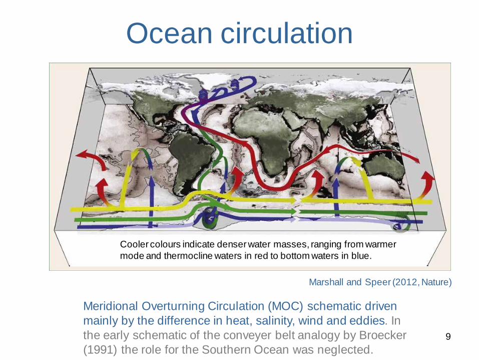
Ocean circulation

9

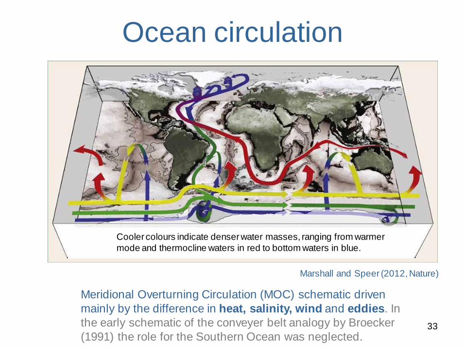
Meridional Overturning Circulation (MOC) schematic driven

mainly by the difference in heat, salinity, wind and eddies. In

the early schematic of the conveyer belt analogy by Broecker

(1991) the role for the Southern Ocean was neglected.

Cooler colours indicate denser water masses, ranging from warmer

mode and thermocline waters in red to bottom waters in blue.

Marshall and Speer (2012, Nature)

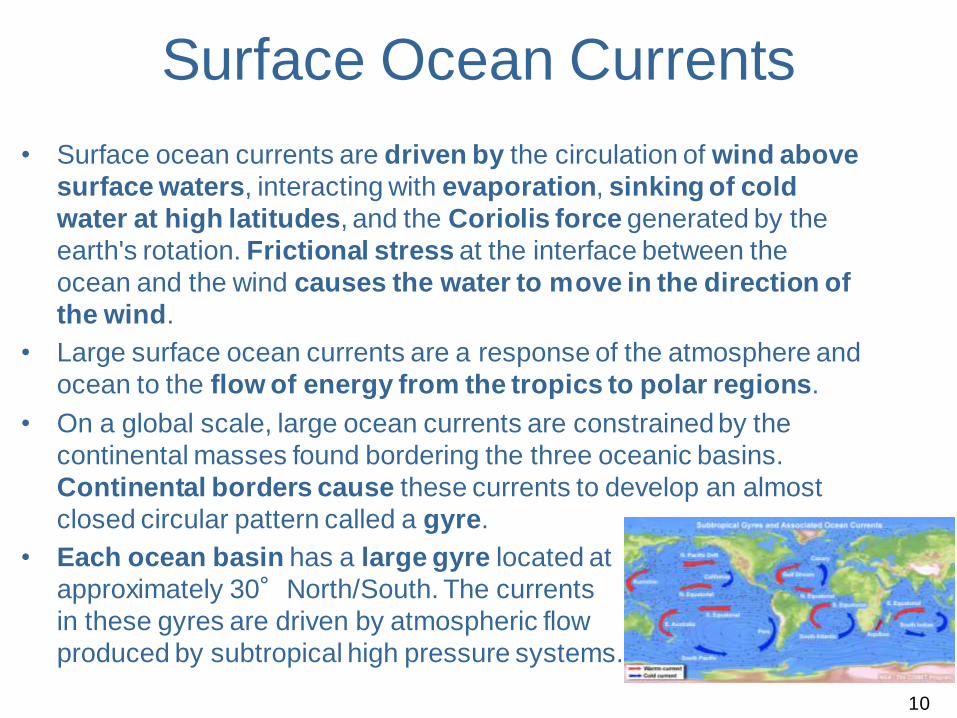
Surface Ocean Currents

• Surface ocean currents are driven by the circulation of wind above

surface waters, interacting with evaporation, sinking of cold

water at high latitudes, and the Coriolis force generated by the

earth's rotation. Frictional stress at the interface between the

ocean and the wind causes the water to move in the direction of

the wind.

• Large surface ocean currents are a response of the atmosphere and

ocean to the flow of energy from the tropics to polar regions.

• On a global scale, large ocean currents are constrained by the

continental masses found bordering the three oceanic basins.

Continental borders cause these currents to develop an almost

closed circular pattern called a gyre.

• Each ocean basin has a large gyre located at

approximately 30°North/South. The currents

in these gyres are driven by atmospheric flow

produced by subtropical high pressure systems.

10

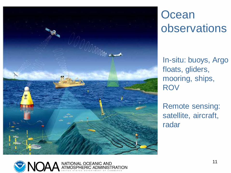
Ocean

observations

11

In-situ: buoys, Argo

floats, gliders,

mooring, ships,

ROV

Remote sensing:

satellite, aircraft,

radar

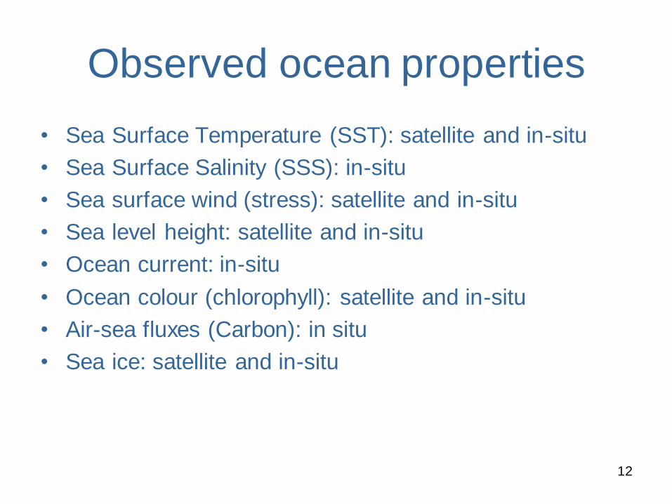
Observed ocean properties

• Sea Surface Temperature (SST): satellite and in-situ

• Sea Surface Salinity (SSS): in-situ

• Sea surface wind (stress): satellite and in-situ

• Sea level height: satellite and in-situ

• Ocean current: in-situ

• Ocean colour (chlorophyll): satellite and in-situ

• Air-sea fluxes (Carbon): in situ

• Sea ice: satellite and in-situ

12

Introduction and Motivation

to Chapter 3

13

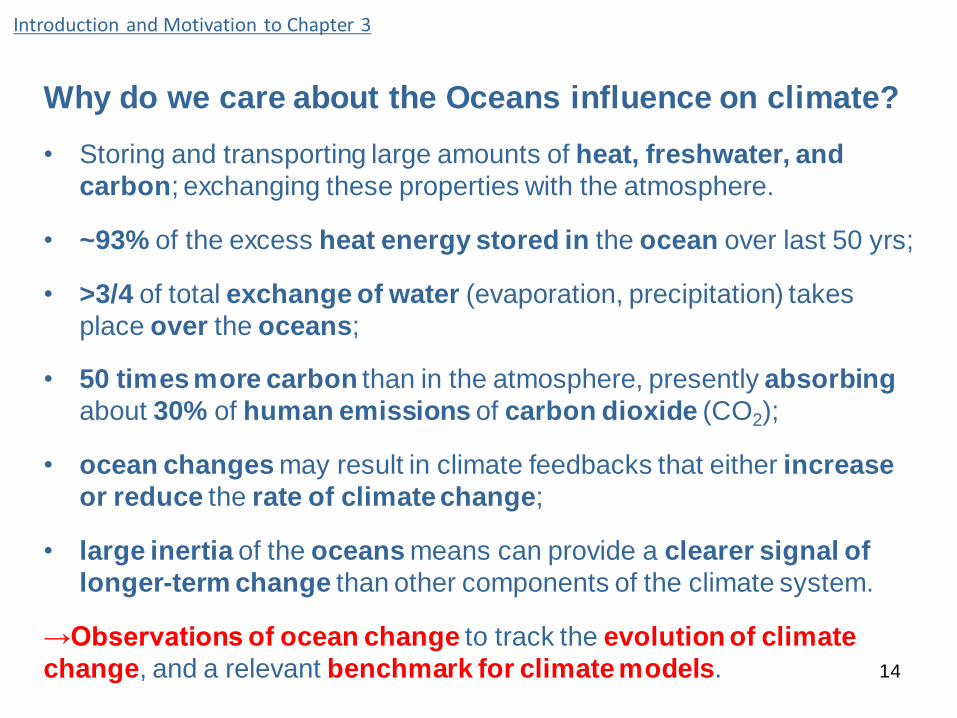
Introduction and Motivation to Chapter 3

Why do we care about the Oceans influence on climate?

• Storing and transporting large amounts of heat, freshwater, and

carbon; exchanging these properties with the atmosphere.

• ~93% of the excess heat energy stored in the ocean over last 50 yrs;

• >3/4 of total exchange of water (evaporation, precipitation) takes

place over the oceans;

• 50 times more carbon than in the atmosphere, presently absorbing

about 30% of human emissions of carbon dioxide (CO2);

• ocean changes may result in climate feedbacks that either increase

or reduce the rate of climate change;

• large inertia of the oceans means can provide a clearer signal of

longer-term change than other components of the climate system.

→Observations of ocean change to track the evolution of climate

change, and a relevant benchmark for climate models. 14

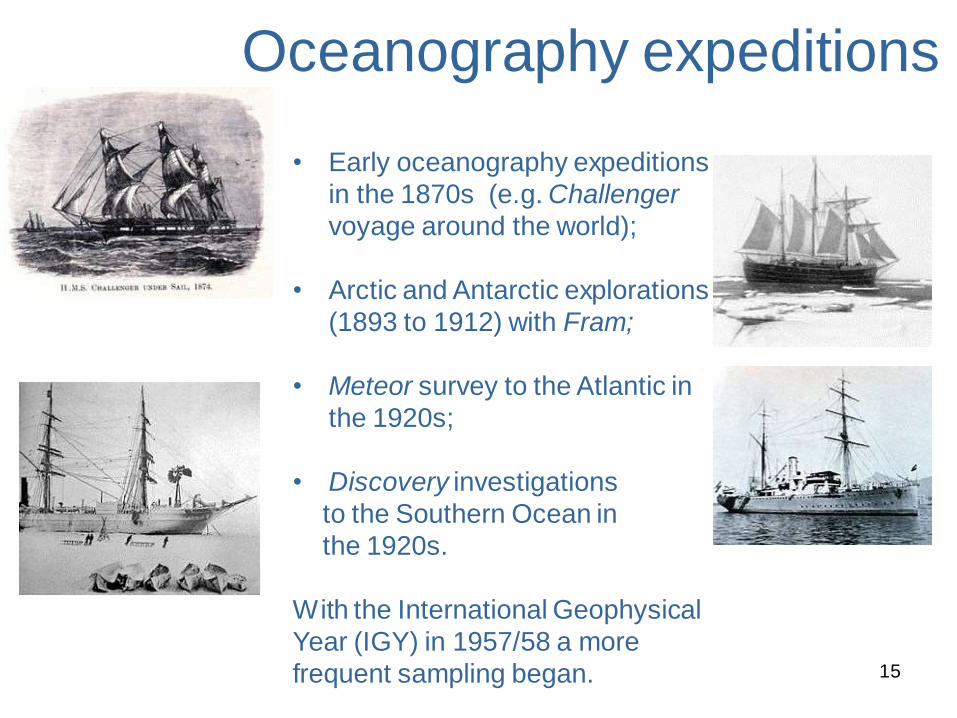
• Early oceanography expeditions

in the 1870s (e.g. Challenger

voyage around the world);

• Arctic and Antarctic explorations

(1893 to 1912) with Fram;

• Meteor survey to the Atlantic in

the 1920s;

• Discovery investigations

to the Southern Ocean in

the 1920s.

With the International Geophysical

Year (IGY) in 1957/58 a more

frequent sampling began.

Oceanography expeditions

15

16

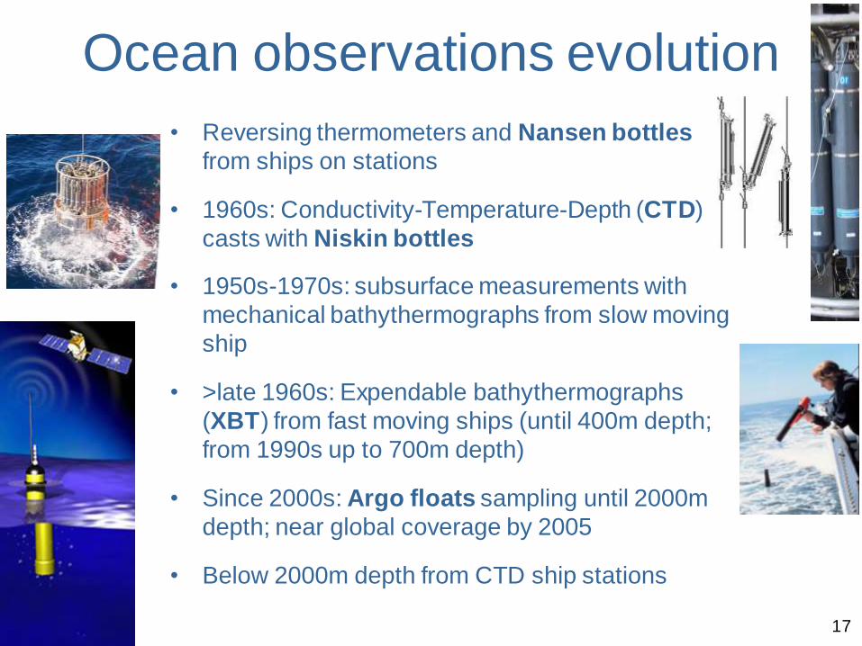
Ocean observations evolution

Ocean observations evolution

• Reversing thermometers and Nansen bottles

from ships on stations

• 1960s: Conductivity-Temperature-Depth (CTD)

casts with Niskin bottles

• 1950s-1970s: subsurface measurements with

mechanical bathythermographs from slow moving

ship

• >late 1960s: Expendable bathythermographs

(XBT) from fast moving ships (until 400m depth;

from 1990s up to 700m depth)

• Since 2000s: Argo floats sampling until 2000m

depth; near global coverage by 2005

• Below 2000m depth from CTD ship stations

17

Ocean observations coverage

18

Ocean observations improvements

since AR4

Lack of long-term ocean measurements → documenting and

understanding oceans changes is an ongoing challenge.

Since AR4, substantial progress has been made in improving the quality

and coverage of ocean observations:

• Biases in historical measurements have been identified and reduced,

providing a clearer record of past change.

• Argo floats have provided near-global, year-round measurements

of temperature and salinity in the upper 2000 m since 2005.

• Satellite altimetry record is now >20 years in length.

• Longer continuous time series of the meridional overturning circulation and

tropical oceans have been obtained.

• Spatial and temporal coverage of biogeochemical measurements in the ocean

has expanded.

→Understanding ocean change has improved. 19

3.2 Ocean temperature and heat content

20

Introduction: Ocean temperature and heat content

“Temperature is the most often measured

subsurface ocean variable.”

• How is the temperature in the shallow,

medium and deep ocean changing?

• How is the ocean heat content changing?

21

-H: Ocean heat content

-ρ: water density -cp: specific heat capacity for sea water -h1,2: ocean depth

-T: Temperature

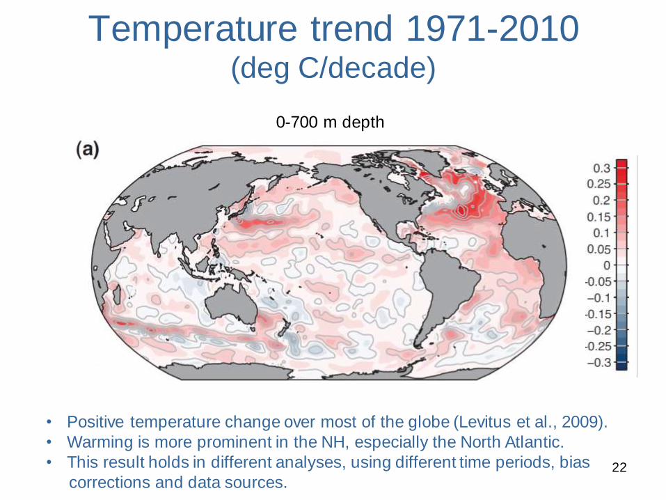
Temperature trend 1971-2010 (deg C/decade)

22

0-700 m depth

• Positive temperature change over most of the globe (Levitus et al., 2009).

• Warming is more prominent in the NH, especially the North Atlantic.

• This result holds in different analyses, using different time periods, bias

corrections and data sources.

23

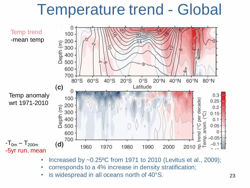
Temperature trend - Global

Temp trend

-mean temp

Temp anomaly

wrt 1971-2010

• Increased by ~0.25ºC from 1971 to 2010 (Levitus et al., 2009); • corresponds to a 4% increase in density stratification;

• is widespread in all oceans north of 40°S.

-T0m – T200m

-5yr run. mean

Why is the Northern Ocean warming stronger than the Southern Ocean?

• Discuss together

25

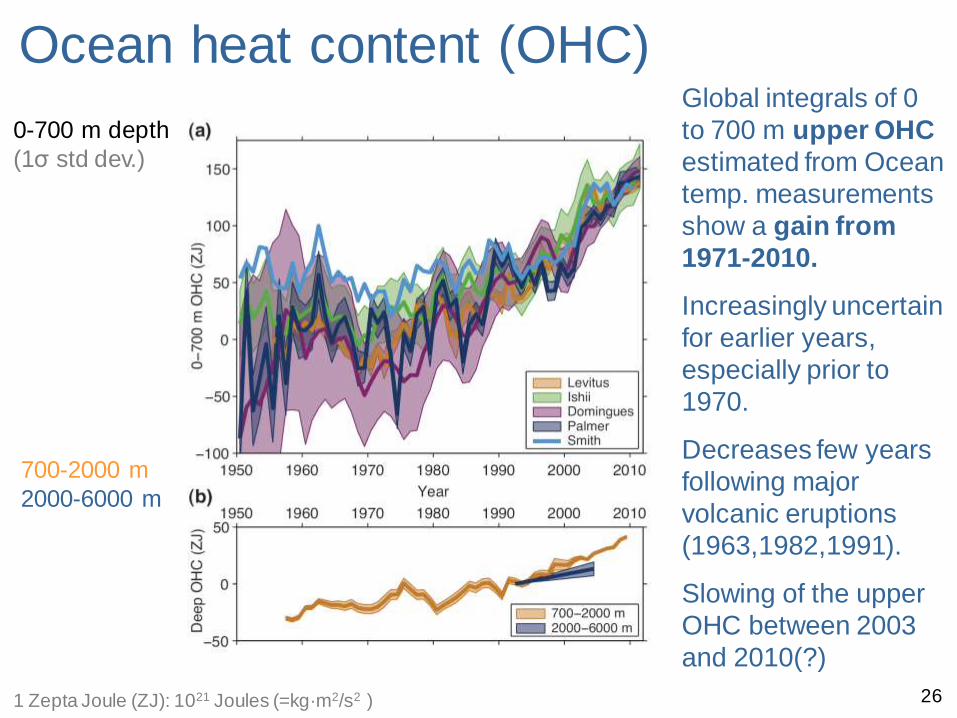
Ocean heat content (OHC)

26 1 Zepta Joule (ZJ): 1021 Joules (=kg·m2/s2 )

0-700 m depth

(1σ std dev.)

700-2000 m

2000-6000 m

Global integrals of 0

to 700 m upper OHC

estimated from Ocean

temp. measurements

show a gain from

1971-2010.

Increasingly uncertain

for earlier years,

especially prior to

1970.

Decreases few years

following major

volcanic eruptions

(1963,1982,1991).

Slowing of the upper

OHC between 2003

and 2010(?)




• Lecture/ interactive seminar/ field excursion Teaching language: English Time and location: see next slide,

CIENS Glasshallen 2.

• Study program



28



29










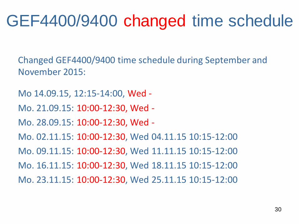
GEF4400/9400 changed time schedule

Changed GEF4400/9400 time schedule during September and November 2015:

Mo 14.09.15, 12:15-14:00, Wed -

Mo. 21.09.15: 10:00-12:30, Wed -

Mo. 28.09.15: 10:00-12:30, Wed -

Mo. 02.11.15: 10:00-12:30, Wed 04.11.15 10:15-12:00

Mo. 09.11.15: 10:00-12:30, Wed 11.11.15 10:15-12:00

Mo. 16.11.15: 10:00-12:30, Wed 18.11.15 10:15-12:00

Mo. 23.11.15: 10:00-12:30, Wed 25.11.15 10:15-12:00

30

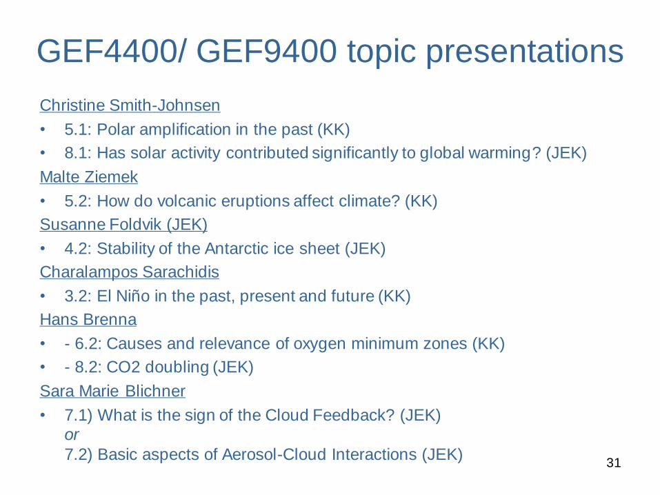
GEF4400/ GEF9400 topic presentations

Christine Smith-Johnsen

• 5.1: Polar amplification in the past (KK)

• 8.1: Has solar activity contributed significantly to global warming? (JEK)

Malte Ziemek

• 5.2: How do volcanic eruptions affect climate? (KK)

Susanne Foldvik (JEK)

• 4.2: Stability of the Antarctic ice sheet (JEK)

Charalampos Sarachidis

• 3.2: El Niño in the past, present and future (KK)

Hans Brenna

• - 6.2: Causes and relevance of oxygen minimum zones (KK)

• - 8.2: CO2 doubling (JEK)

Sara Marie Blichner

• 7.1) What is the sign of the Cloud Feedback? (JEK) or

7.2) Basic aspects of Aerosol-Cloud Interactions (JEK)

31

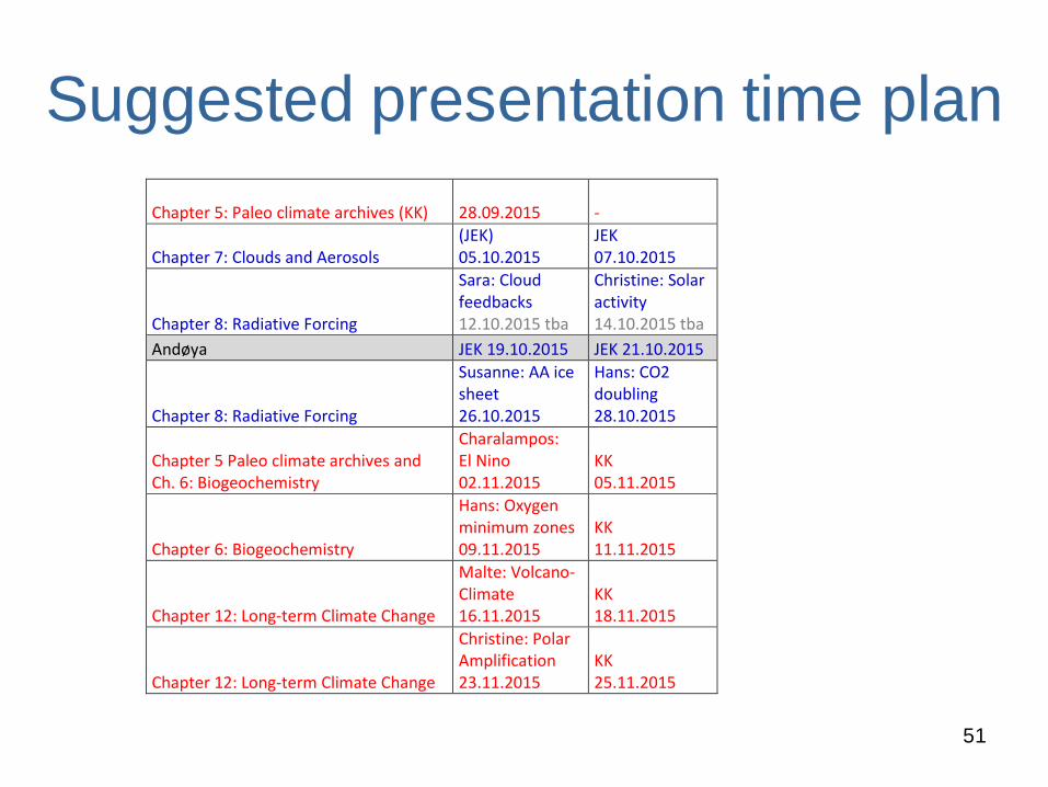
Suggested presentation time plan

32

Chapter 5: Paleo climate archives (KK) 28.09.2015 -

Chapter 7: Clouds and Aerosols (JEK) 05.10.2015

JEK 07.10.2015

Chapter 8: Radiative Forcing

Sara: Cloud feedbacks

12.10.2015 tba

Christine: Solar activity

14.10.2015 tba

Andøya JEK 19.10.2015 JEK 21.10.2015


Susanne: AA ice sheet 26.10.2015

Hans: CO2 doubling 28.10.2015

Chapter 5 Paleo climate archives and Ch. 6: Biogeochemistry

Charalampos: El Nino 02.11.2015

KK 05.11.2015

Chapter 6: Biogeochemistry

Hans: Oxygen minimum zones 09.11.2015

KK 11.11.2015

Chapter 12: Long-term Climate Change

Malte: Volcano-Climate 16.11.2015

KK 18.11.2015


Christine: Polar Amplification 23.11.2015

KK 25.11.2015

Ocean circulation

33

Meridional Overturning Circulation (MOC) schematic driven

mainly by the difference in heat, salinity, wind and eddies. In

the early schematic of the conveyer belt analogy by Broecker

(1991) the role for the Southern Ocean was neglected.

Cooler colours indicate denser water masses, ranging from warmer

mode and thermocline waters in red to bottom waters in blue.

Marshall and Speer (2012, Nature)

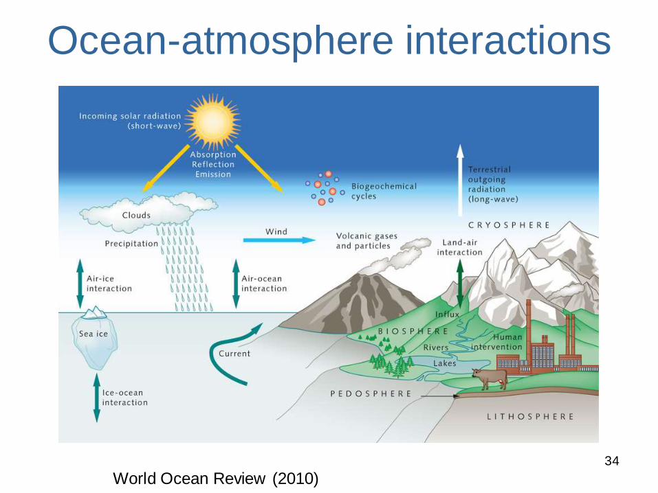
Ocean-atmosphere interactions

34

World Ocean Review (2010)

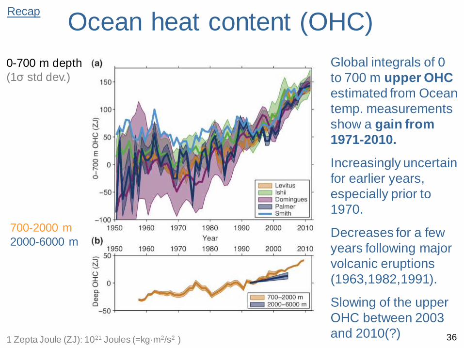
Ocean heat content (OHC)

36 1 Zepta Joule (ZJ): 1021 Joules (=kg·m2/s2 )

0-700 m depth

(1σ std dev.)

700-2000 m

2000-6000 m

Global integrals of 0

to 700 m upper OHC

estimated from Ocean

temp. measurements

show a gain from

1971-2010.

Increasingly uncertain

for earlier years,

especially prior to

1970.

Decreases for a few

years following major

volcanic eruptions

(1963,1982,1991).

Slowing of the upper

OHC between 2003

and 2010(?)

Recap

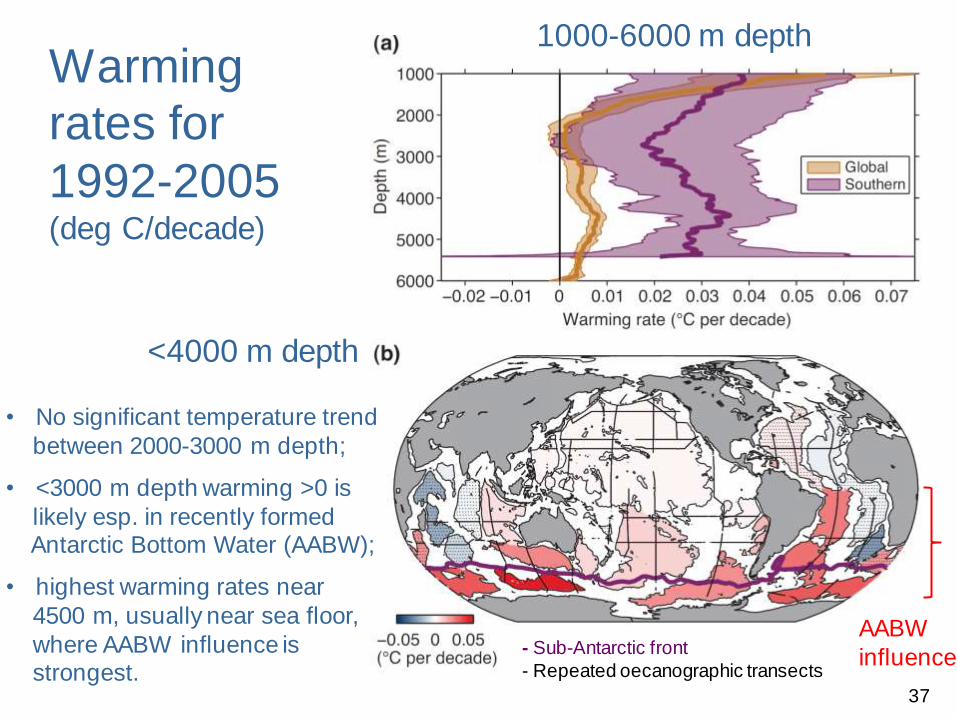
Warming

rates for

1992-2005 (deg C/decade)

37

<4000 m depth

- Sub-Antarctic front

- Repeated oecanographic transects

• No significant temperature trend

between 2000-3000 m depth;

• <3000 m depth warming >0 is

likely esp. in recently formed Antarctic Bottom Water (AABW);

• highest warming rates near

4500 m, usually near sea floor,

where AABW influence is strongest.

AABW

influence

1000-6000 m depth

Why is the AABW warming?

• Discuss together…

• …

• …

38

39

Chapter 4, WMO Ozone Assessment (2015)

Stratospheric O3 depletion > strengthening westerly winds (positive

Southern Annular Mode) > increased surface wind stress > strengthening

overturning circulation of the Southern Ocean

41

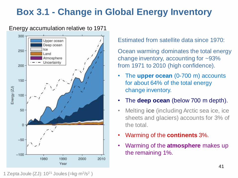
Estimated from satellite data since 1970:

Ocean warming dominates the total energy

change inventory, accounting for ~93%

from 1971 to 2010 (high confidence).

• The upper ocean (0-700 m) accounts

for about 64% of the total energy

change inventory.

• The deep ocean (below 700 m depth).

• Melting ice (including Arctic sea ice, ice

sheets and glaciers) accounts for 3% of

the total.

• Warming of the continents 3%.

• Warming of the atmosphere makes up

the remaining 1%.

1 Zepta Joule (ZJ): 1021 Joules (=kg·m2/s2 )

Box 3.1 - Change in Global Energy Inventory

Energy accumulation relative to 1971

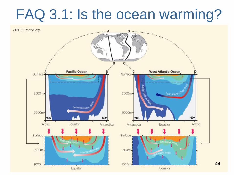
FAQ 3.1: Is the ocean warming?

43

First, let’s discuss in groups pro’s and con’s.

• “Yes, the ocean is warming over many regions, depth ranges and

time periods,

• although neither everywhere nor constantly.

• The signature of warming emerges most clearly when considering

global, or even ocean basin, averages over time spans of a decade

or more.

• Ocean temperature at any given location can vary greatly with the

seasons.

• It can also fluctuate substantially from year to year - or even

decade to decade - because of variations in ocean currents and

the exchange of heat between ocean and atmosphere.”

FAQ 3.1: Is the ocean warming?

44

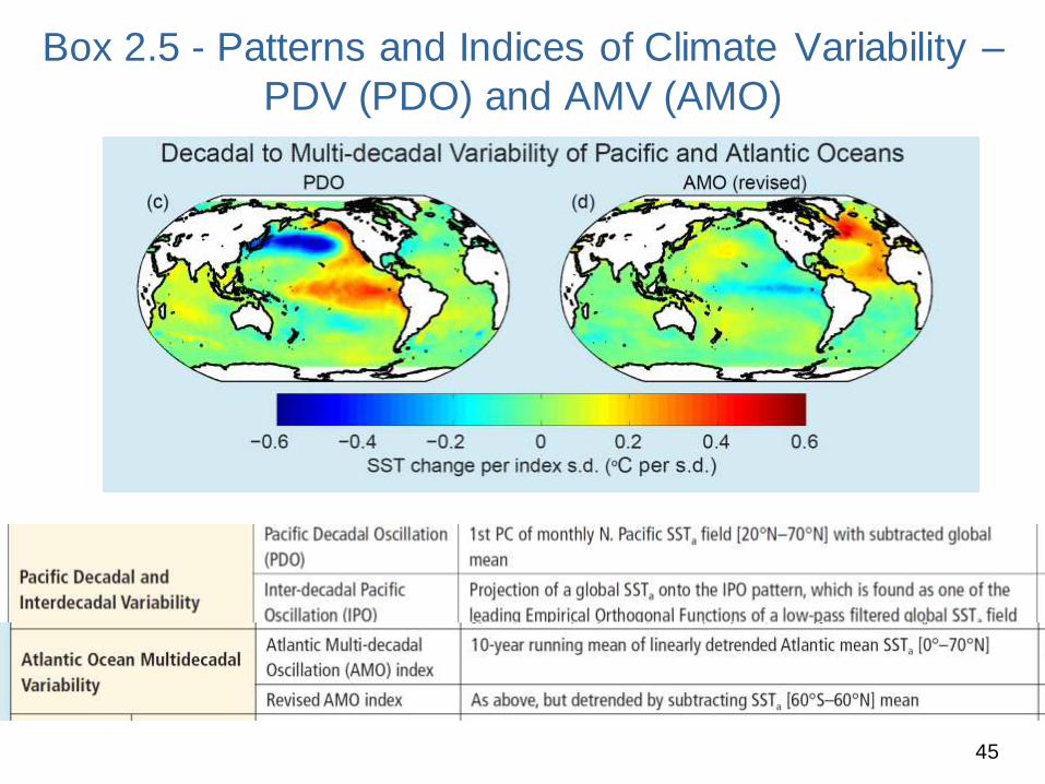
Box 2.5 - Patterns and Indices of Climate Variability –

PDV (PDO) and AMV (AMO)

45

Box 2.5 - Patterns and Indices of Climate Variability -

PDV and AMV

46 HadISST: Hadley Centre Sea Ice and Sea Surface Temperature data set; Rayner et al (2003, JGR)

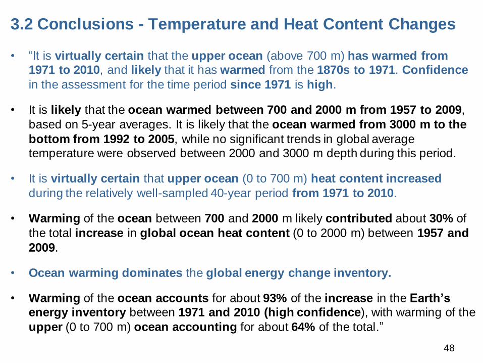
3.2 Conclusions - Temperature and Heat Content Changes

• “It is virtually certain that the upper ocean (above 700 m) has warmed from 1971 to 2010, and likely that it has warmed from the 1870s to 1971. Confidence

in the assessment for the time period since 1971 is high.

• It is likely that the ocean warmed between 700 and 2000 m from 1957 to 2009,

based on 5-year averages. It is likely that the ocean warmed from 3000 m to the

bottom from 1992 to 2005, while no significant trends in global average temperature were observed between 2000 and 3000 m depth during this period.

• It is virtually certain that upper ocean (0 to 700 m) heat content increased

during the relatively well-sampled 40-year period from 1971 to 2010.

• Warming of the ocean between 700 and 2000 m likely contributed about 30% of

the total increase in global ocean heat content (0 to 2000 m) between 1957 and

2009.

• Ocean warming dominates the global energy change inventory.

• Warming of the ocean accounts for about 93% of the increase in the Earth’s energy inventory between 1971 and 2010 (high confidence), with warming of the

upper (0 to 700 m) ocean accounting for about 64% of the total.”

48




• Lecture/ interactive seminar/ field excursion Teaching language: English Time and location: see next slide,

CIENS Glasshallen 2.

• Study program



49



50










Suggested presentation time plan

51

Chapter 5: Paleo climate archives (KK) 28.09.2015 -

Chapter 7: Clouds and Aerosols (JEK) 05.10.2015

JEK 07.10.2015


Sara: Cloud feedbacks

12.10.2015 tba

Christine: Solar activity

14.10.2015 tba

Andøya JEK 19.10.2015 JEK 21.10.2015


Susanne: AA ice sheet 26.10.2015

Hans: CO2 doubling 28.10.2015

Chapter 5 Paleo climate archives and Ch. 6: Biogeochemistry

Charalampos: El Nino 02.11.2015

KK 05.11.2015

Chapter 6: Biogeochemistry

Hans: Oxygen minimum zones 09.11.2015

KK 11.11.2015


Malte: Volcano-Climate 16.11.2015

KK 18.11.2015


Christine: Polar Amplification 23.11.2015

KK 25.11.2015

3.3 Salinity and fresh water

content

52

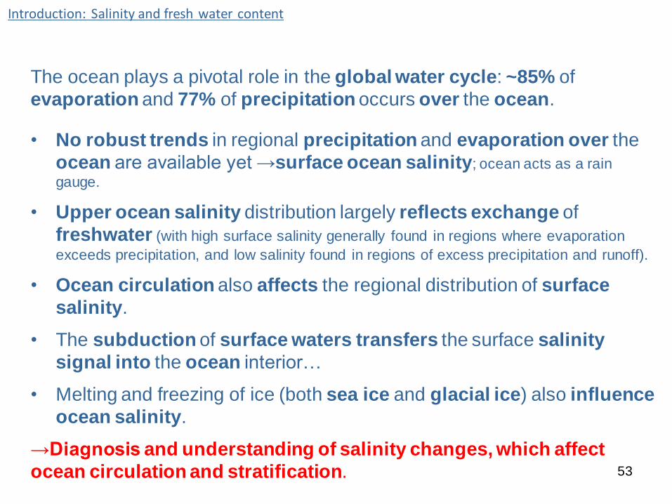
Introduction: Salinity and fresh water content

The ocean plays a pivotal role in the global water cycle: ~85% of

evaporation and 77% of precipitation occurs over the ocean.

• No robust trends in regional precipitation and evaporation over the

ocean are available yet →surface ocean salinity; ocean acts as a rain

gauge.

• Upper ocean salinity distribution largely reflects exchange of

freshwater (with high surface salinity generally found in regions where evaporation

exceeds precipitation, and low salinity found in regions of excess precipitation and runoff).

• Ocean circulation also affects the regional distribution of surface

salinity.

• The subduction of surface waters transfers the surface salinity

signal into the ocean interior…

• Melting and freezing of ice (both sea ice and glacial ice) also influence

ocean salinity.

→Diagnosis and understanding of salinity changes, which affect

ocean circulation and stratification. 53

Salinity

• “‘Salinity’ refers to the weight of dissolved salts

in a kilogram of seawater. Because the total

amount of salt in the ocean does not change, the

salinity of seawater can be changed only by

addition or removal of fresh water. All salinity

values quoted in the chapter are expressed on

the Practical Salinity Scale 1978 (PSS78*)

(Lewis and Fofonoff, 1979).”

54

*PSS-78: Practical Salinity Scale 1978 is based on an equation relating

salinity to the ratio of the electrical conductivity of seawater at 15°C to that of

a standard potassium chloride solution (KCl).

• In AR4, surface and subsurface salinity changes consistent with a

warmer climate were highlighted…

• In the early few decades the salinity data distribution was good

in the NH, but the coverage was poor in some regions such as the

central South Pacific, central Indian and polar oceans.

• Argo provides much more even spatial and temporal coverage

in the 2000s.

→Additional observations, improvements in the availability and

quality of historical data and new analysis approaches now allow a

more complete AR5 assessment of changes in salinity.

55

Salinity observations improvements

since AR4

AR4/5: IPCC assessment report No. 4/5 published in 2007/2013.

Salinity and E-P Climatologies

56

Sea surface

salinity (SSS)

mean 1955-2005

Evaporation-

Precipitation

(E-P) 1950-2000

- Maxima in evaporation-dominated subtropical gyres.

- Minima at subpolar lat and ITCZ.

- Interbasin differences: Atlantic more saline, Pacific more fresh.

SSS: World Ocean Atlas (WOA) 1955-2005 data

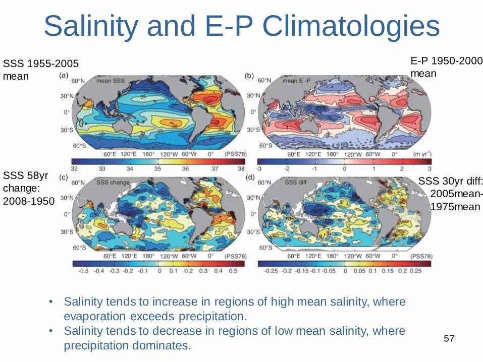
Salinity and E-P Climatologies

57

SSS 1955-2005

mean

SSS 58yr

change:

2008-1950

SSS 30yr diff:

2005mean-

1975mean

E-P 1950-2000

mean

• Salinity tends to increase in regions of high mean salinity, where

evaporation exceeds precipitation.

• Salinity tends to decrease in regions of low mean salinity, where

precipitation dominates.

59

FAQ 3.2: Is There Evidence for Changes

in the Earth’s Water Cycle?

Special Sensor Microwave

Imager satellite observations (Wentz et al 2007)

1979-2005 NCEP/NCAR

reanalysis (Kalnay et al 1996)

Surface salinity (PSS78)

after Durack and Wijffels (2010)

• Changes in the atmosphere’s

water vapour content provide

strong evidence that the water

cycle is already responding to

a warming climate.

• Further evidence comes from

changes in the distribution of

ocean salinity,

• Observations since the 1970s

show increases in surface and lower atmospheric water

vapour at a rate consistent with

observed warming (~7% H2O

increase /1 deg C).

• Moreover, evaporation and precipitation are projected to

intensify in a warmer climate.

wetter

drier

Net

-precip. -evap.

freshening

saltier

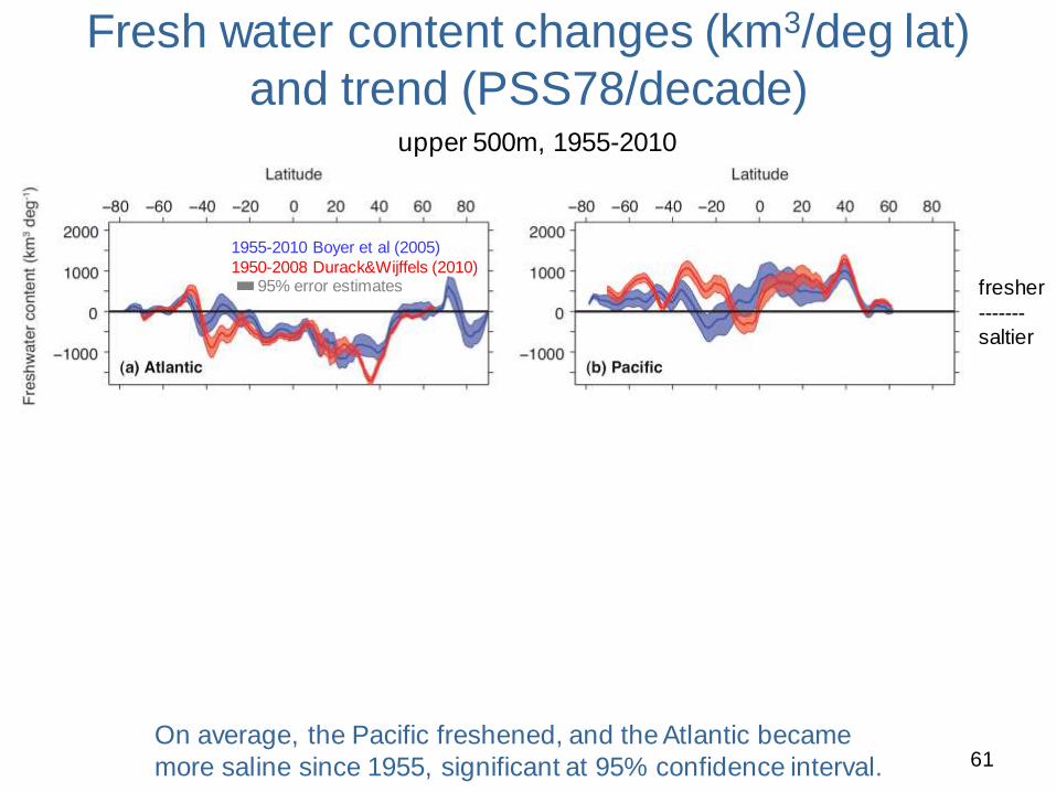
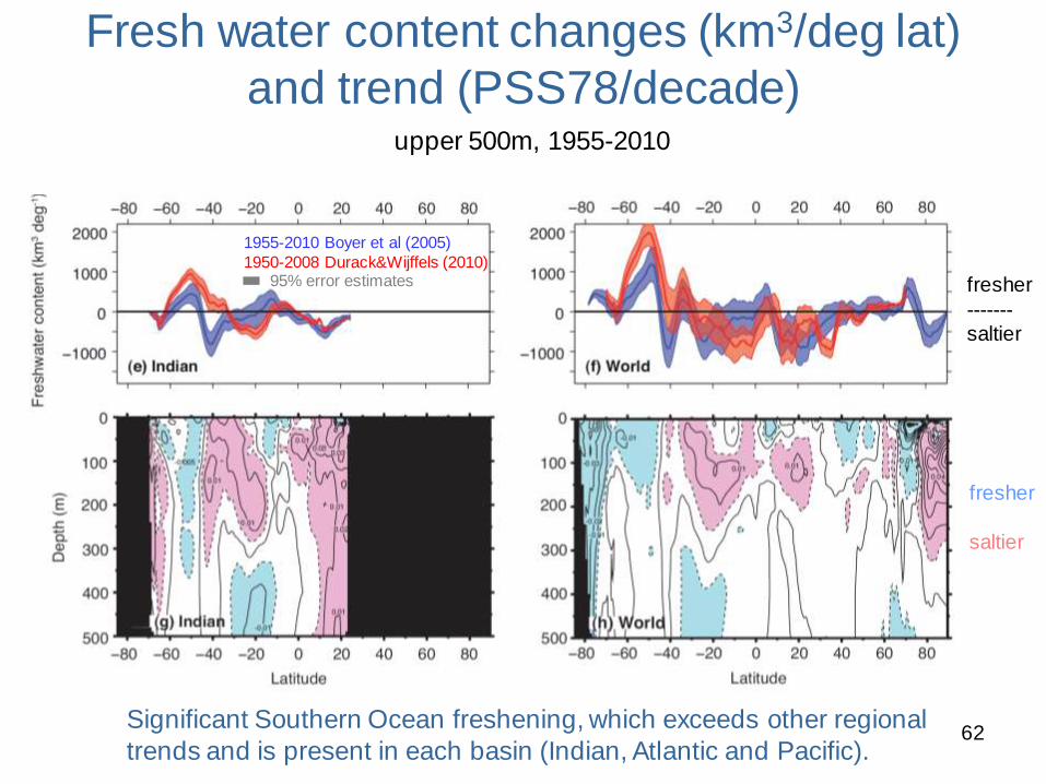
Fresh water content changes (km3/deg lat)

and trend (PSS78/decade)

61

upper 500m, 1955-2010

1955-2010 Boyer et al (2005)

1950-2008 Durack&Wijffels (2010) 95% error estimates fresher

------- saltier

fresher

saltier

On average, the Pacific freshened, and the Atlantic became

more saline since 1955, significant at 95% confidence interval.

62

upper 500m, 1955-2010

1955-2010 Boyer et al (2005)

1950-2008 Durack&Wijffels (2010) 95% error estimates

Fresh water content changes (km3/deg lat)

and trend (PSS78/decade)

fresher

------- saltier

fresher

saltier

Significant Southern Ocean freshening, which exceeds other regional

trends and is present in each basin (Indian, Atlantic and Pacific).

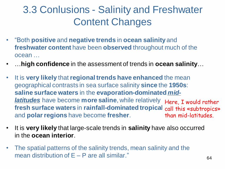
3.3 Conlusions - Salinity and Freshwater

Content Changes

• “Both positive and negative trends in ocean salinity and

freshwater content have been observed throughout much of the

ocean …

• …high confidence in the assessment of trends in ocean salinity…

• It is very likely that regional trends have enhanced the mean

geographical contrasts in sea surface salinity since the 1950s:

saline surface waters in the evaporation-dominated mid-

latitudes have become more saline, while relatively

fresh surface waters in rainfall-dominated tropical

and polar regions have become fresher.

• It is very likely that large-scale trends in salinity have also occurred

in the ocean interior.

• The spatial patterns of the salinity trends, mean salinity and the

mean distribution of E – P are all similar.”

64

Here, I would rather call this «subtropics» than mid-latitudes.

3.4 Ocean surface fluxes

65

Introduction: Ocean surface fluxes

Relevance of

ocean surface

fluxes:

• “Exchanges of heat,

water and momentum (wind stress) at the sea

surface are important

factors for driving the

ocean circulation.

66

• Changes in the air–sea fluxes may result from variations in the driving surface

meteorological state variables (air temperature and humidity, SST, wind speed, cloud cover,

precipitation) and can impact both water-mass formation rates and ocean circulation.

• Air–sea fluxes also influence temperature and humidity in the atmosphere and,

therefore, the hydrological cycle and atmospheric circulation.

• The net air–sea heat flux is the sum of two turbulent (latent and sensible)

and two radiative (shortwave and longwave) components.”

www.whoi.edu

• “AR4 concluded that, at the global scale, the accuracy of the

observations is insufficient to permit a direct assessment of

changes in heat flux...

• …although substantial progress has been made since AR4, that

conclusion still holds for this assessment.”

67

Ocean surface fluxes - improvements

since AR4

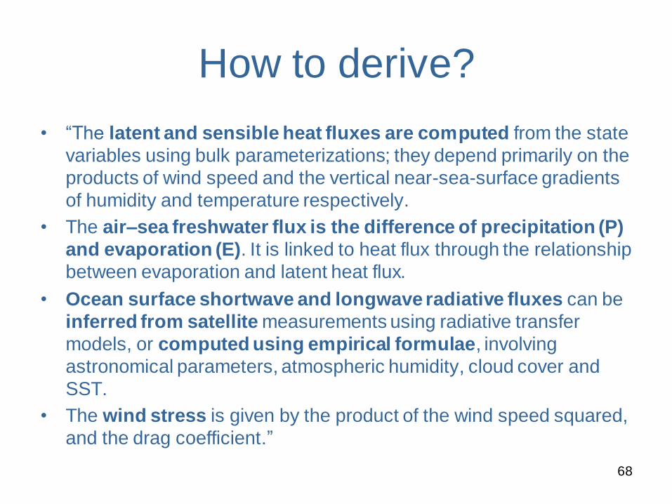
How to derive?

• “The latent and sensible heat fluxes are computed from the state

variables using bulk parameterizations; they depend primarily on the

products of wind speed and the vertical near-sea-surface gradients

of humidity and temperature respectively.

• The air–sea freshwater flux is the difference of precipitation (P)

and evaporation (E). It is linked to heat flux through the relationship

between evaporation and latent heat flux.

• Ocean surface shortwave and longwave radiative fluxes can be

inferred from satellite measurements using radiative transfer

models, or computed using empirical formulae, involving

astronomical parameters, atmospheric humidity, cloud cover and

SST.

• The wind stress is given by the product of the wind speed squared,

and the drag coefficient.”

68

Box 2.3 – Global Atmospheric Reanalyses

69

• MERRA and ERA-Interim reanalyses show improved tropical precipitation and

hence better represent the global hydrological cycle (Dee et al., 2011b).

• The NCEP/CFSR reanalysis uses a coupled ocean–atmosphere–land-sea–ice

model (Saha et al., 2010).

• 20CR (Compo et al., 2011) is a 56-member ensemble and covers 140 years by

assimilating only surface and sea level pressure (SLP) information.

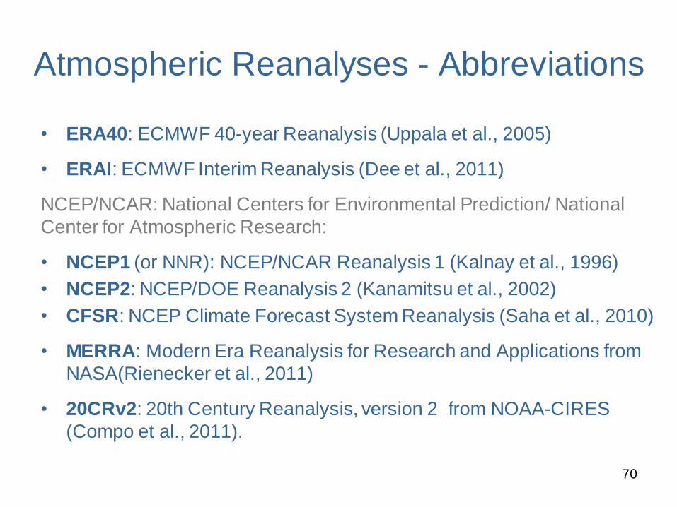
Atmospheric Reanalyses - Abbreviations

• ERA40: ECMWF 40-year Reanalysis (Uppala et al., 2005)

• ERAI: ECMWF Interim Reanalysis (Dee et al., 2011)

NCEP/NCAR: National Centers for Environmental Prediction/ National

Center for Atmospheric Research:

• NCEP1 (or NNR): NCEP/NCAR Reanalysis 1 (Kalnay et al., 1996)

• NCEP2: NCEP/DOE Reanalysis 2 (Kanamitsu et al., 2002)

• CFSR: NCEP Climate Forecast System Reanalysis (Saha et al., 2010)

• MERRA: Modern Era Reanalysis for Research and Applications from

NASA(Rienecker et al., 2011)

• 20CRv2: 20th Century Reanalysis, version 2 from NOAA-CIRES

(Compo et al., 2011).

70

Ocean evaporation

and surface fluxes

71

• “Analysis of OAFlux suggests that global

mean evaporation may vary at inter-

decadal time scales, with the variability

being relatively small compared to the

mean (Fig. a).

• Changing data sources …may

contribute to this variability …

• The latent heat flux variations (Fig. b) closely follow those in evaporation

(negative values of latent heat flux

corresponding to positive values of

evaporation).”

OAFlux: Objectively Analysed Air–Sea heat flux data

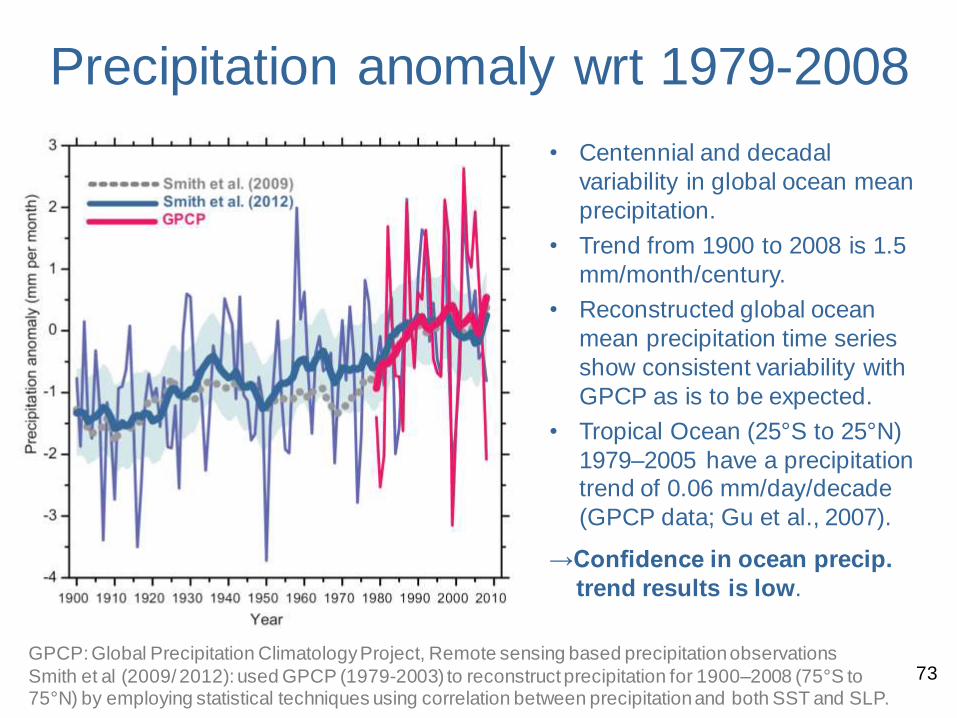
Precipitation anomaly wrt 1979-2008

73 GPCP: Global Precipitation Climatology Project, Remote sensing based precipitation observations

Smith et al (2009/ 2012): used GPCP (1979-2003) to reconstruct precipitation for 1900–2008 (75°S to 75°N) by employing statistical techniques using correlation between precipitation and both SST and SLP.

• Centennial and decadal

variability in global ocean mean

precipitation.

• Trend from 1900 to 2008 is 1.5

mm/month/century.

• Reconstructed global ocean

mean precipitation time series

show consistent variability with

GPCP as is to be expected.

• Tropical Ocean (25°S to 25°N)

1979–2005 have a precipitation trend of 0.06 mm/day/decade

(GPCP data; Gu et al., 2007).

→Confidence in ocean precip.

trend results is low.

Zonal wind stress: Southern Ocean (SO)

75

----Reanalyses

▬ Mean

• Increase in the annual mean zonal wind stress;

• Upward trend from 0.15 N m–2 in early 1950s to 0.20 N m–2 in early 2010s.

• Wind stress strengthening has a seasonal dependence, with strongest trends in

January, linked to changes (upward trend) in the Southern Annular Mode (SAM).

→Medium confidence that SO wind stress has strengthened since 1980s.

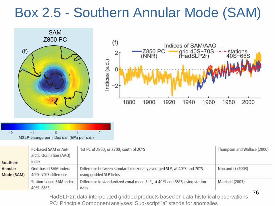
Box 2.5 - Southern Annular Mode (SAM)

76 HadSLP2r: data interpolated gridded products based on data historical observations

PC: Principle Component analyses; Sub-script “a” stands for anomalies

3.4 Conclusions - Air–Sea Flux

• “Uncertainties in air–sea heat flux data sets are too

large to allow detection of the change in global mean

net air-sea heat flux, of the order of 0.5 W m–2 since

1971, required for consistency with the observed ocean

heat content increase.

• Basin-scale wind stress trends at decadal to

centennial time scales have been observed in the North

Atlantic, Tropical Pacific and Southern Ocean with low

to medium confidence.”

77

3.6 Changes in Ocean circulation

78

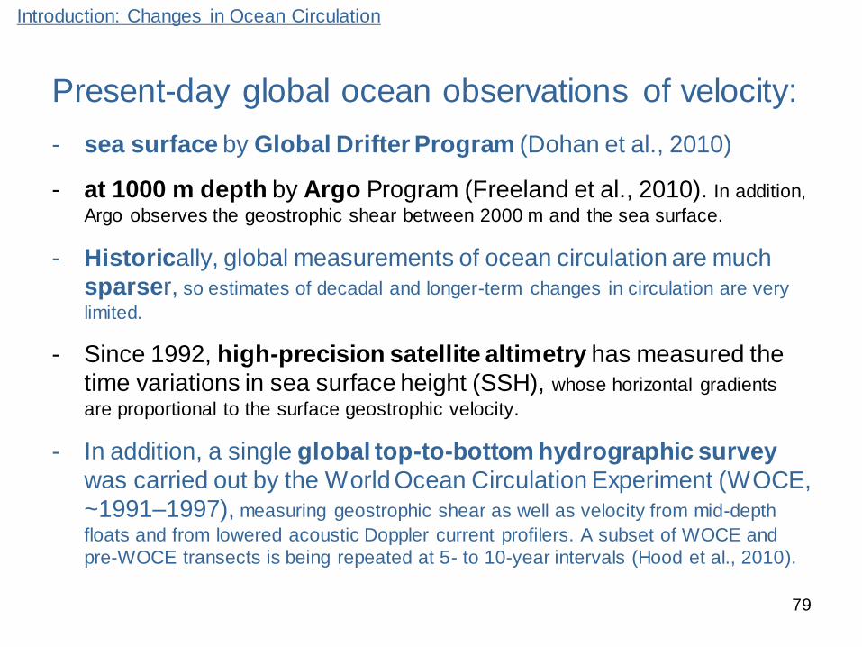
Introduction: Changes in Ocean Circulation

Present-day global ocean observations of velocity:

- sea surface by Global Drifter Program (Dohan et al., 2010)

- at 1000 m depth by Argo Program (Freeland et al., 2010). In addition,

Argo observes the geostrophic shear between 2000 m and the sea surface.

- Historically, global measurements of ocean circulation are much

sparser, so estimates of decadal and longer-term changes in circulation are very

limited.

- Since 1992, high-precision satellite altimetry has measured the

time variations in sea surface height (SSH), whose horizontal gradients

are proportional to the surface geostrophic velocity.

- In addition, a single global top-to-bottom hydrographic survey

was carried out by the World Ocean Circulation Experiment (WOCE,

~1991–1997), measuring geostrophic shear as well as velocity from mid-depth

floats and from lowered acoustic Doppler current profilers. A subset of WOCE and

pre-WOCE transects is being repeated at 5- to 10-year intervals (Hood et al., 2010).

79

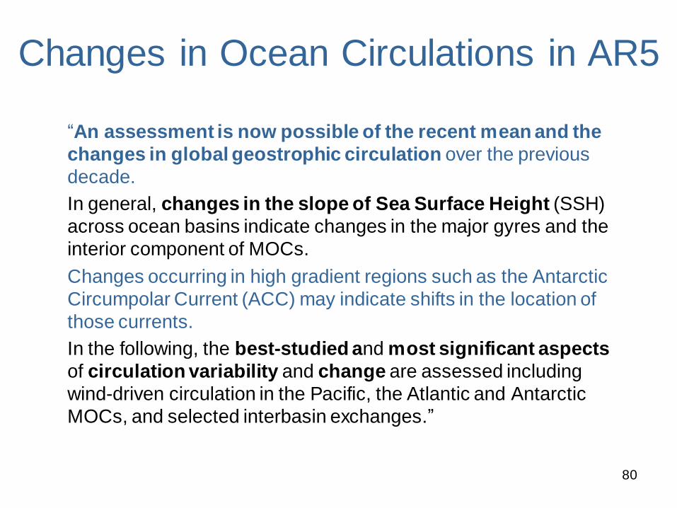
“An assessment is now possible of the recent mean and the

changes in global geostrophic circulation over the previous

decade.

In general, changes in the slope of Sea Surface Height (SSH)

across ocean basins indicate changes in the major gyres and the

interior component of MOCs.

Changes occurring in high gradient regions such as the Antarctic

Circumpolar Current (ACC) may indicate shifts in the location of

those currents.

In the following, the best-studied and most significant aspects

of circulation variability and change are assessed including

wind-driven circulation in the Pacific, the Atlantic and Antarctic

MOCs, and selected interbasin exchanges.”

80

Changes in Ocean Circulations in AR5

81

─m

ean s

teric h

eig

ht o

f se

a s

urf

ace

with

resp

ect t

o the

20

00

de

cib

ars

(in

10

cm

in

terv

als

), A

rgo

20

04

-201

2 d

ata

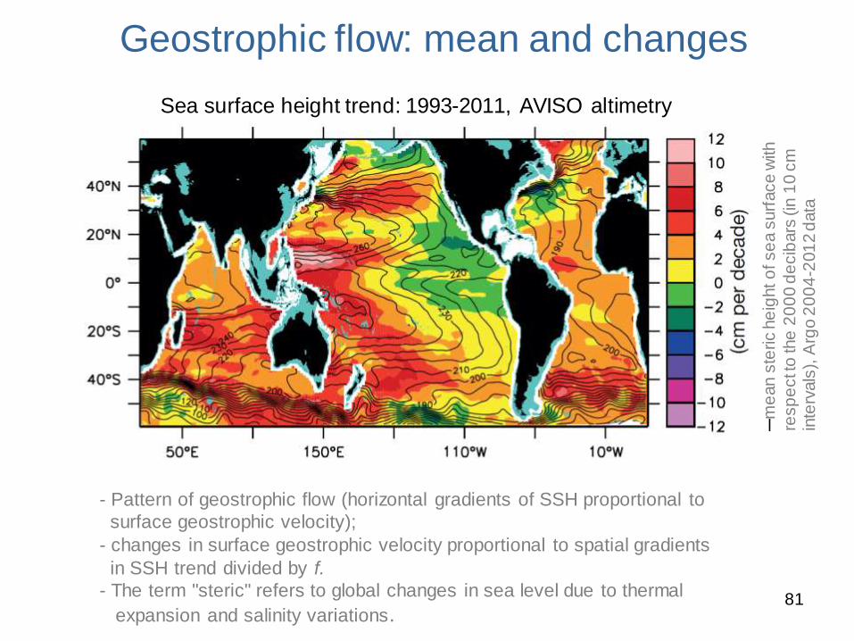
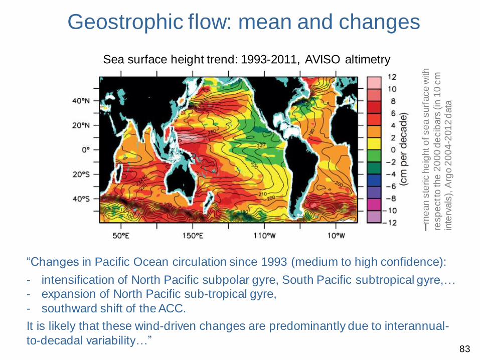
Geostrophic flow: mean and changes

Sea surface height trend: 1993-2011, AVISO altimetry

- Pattern of geostrophic flow (horizontal gradients of SSH proportional to

surface geostrophic velocity);

- changes in surface geostrophic velocity proportional to spatial gradients

in SSH trend divided by f.

- The term "steric" refers to global changes in sea level due to thermal

expansion and salinity variations.

83

─m

ean s

teric h

eig

ht o

f se

a s

urf

ace

with

resp

ect t

o the

20

00

de

cib

ars

(in

10

cm

in

terv

als

), A

rgo

20

04

-201

2 d

ata

Geostrophic flow: mean and changes

Sea surface height trend: 1993-2011, AVISO altimetry

“Changes in Pacific Ocean circulation since 1993 (medium to high confidence):

- intensification of North Pacific subpolar gyre, South Pacific subtropical gyre,… - expansion of North Pacific sub-tropical gyre,

- southward shift of the ACC.

It is likely that these wind-driven changes are predominantly due to interannual-

to-decadal variability…”

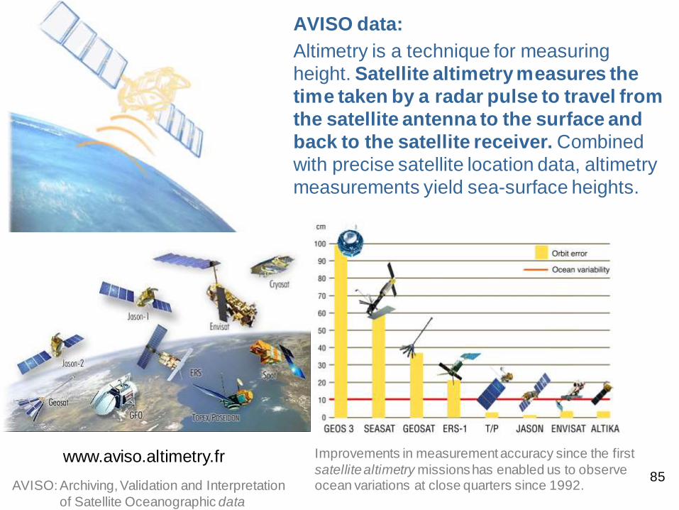
AVISO data:

Altimetry is a technique for measuring

height. Satellite altimetry measures the

time taken by a radar pulse to travel from

the satellite antenna to the surface and

back to the satellite receiver. Combined

with precise satellite location data, altimetry

measurements yield sea-surface heights.

85

Improvements in measurement accuracy since the first

satellite altimetry missions has enabled us to observe ocean variations at close quarters since 1992.

www.aviso.altimetry.fr

AVISO: Archiving, Validation and Interpretation

of Satellite Oceanographic data

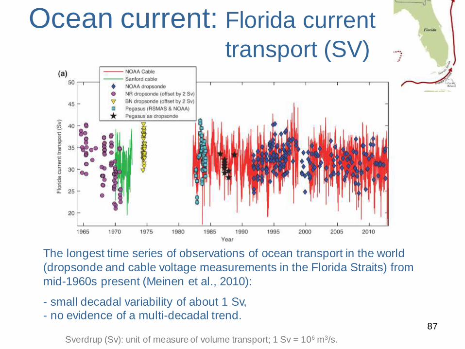
http://www.aviso.altimetry.fr/en/techniques/doris.html

Ocean current: Florida current

transport (SV)

87

Sverdrup (Sv): unit of measure of volume transport; 1 Sv = 106 m3/s.

The longest time series of observations of ocean transport in the world

(dropsonde and cable voltage measurements in the Florida Straits) from

mid-1960s present (Meinen et al., 2010):

- small decadal variability of about 1 Sv, - no evidence of a multi-decadal trend.

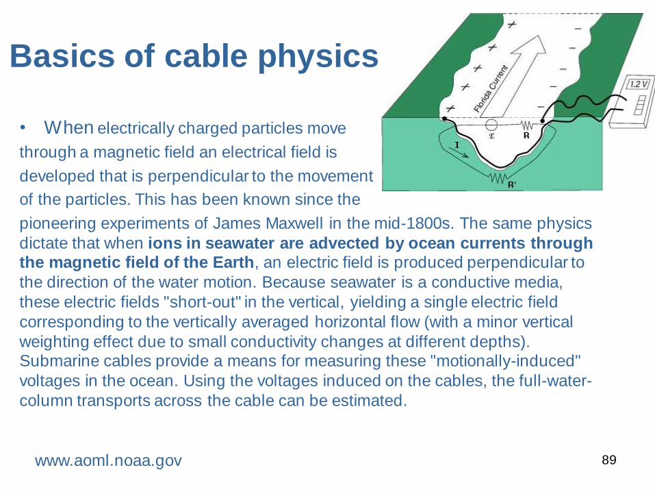
Basics of cable physics:

• When electrically charged particles move

through a magnetic field an electrical field is

developed that is perpendicular to the movement

of the particles. This has been known since the

pioneering experiments of James Maxwell in the mid-1800s. The same physics

dictate that when ions in seawater are advected by ocean currents through the magnetic field of the Earth, an electric field is produced perpendicular to

the direction of the water motion. Because seawater is a conductive media,

these electric fields "short-out" in the vertical, yielding a single electric field

corresponding to the vertically averaged horizontal flow (with a minor vertical

weighting effect due to small conductivity changes at different depths). Submarine cables provide a means for measuring these "motionally-induced"

voltages in the ocean. Using the voltages induced on the cables, the full-water-

column transports across the cable can be estimated.

89 www.aoml.noaa.gov

Atlantic Meridional Overturning Circulation:

AMOC transport estimates

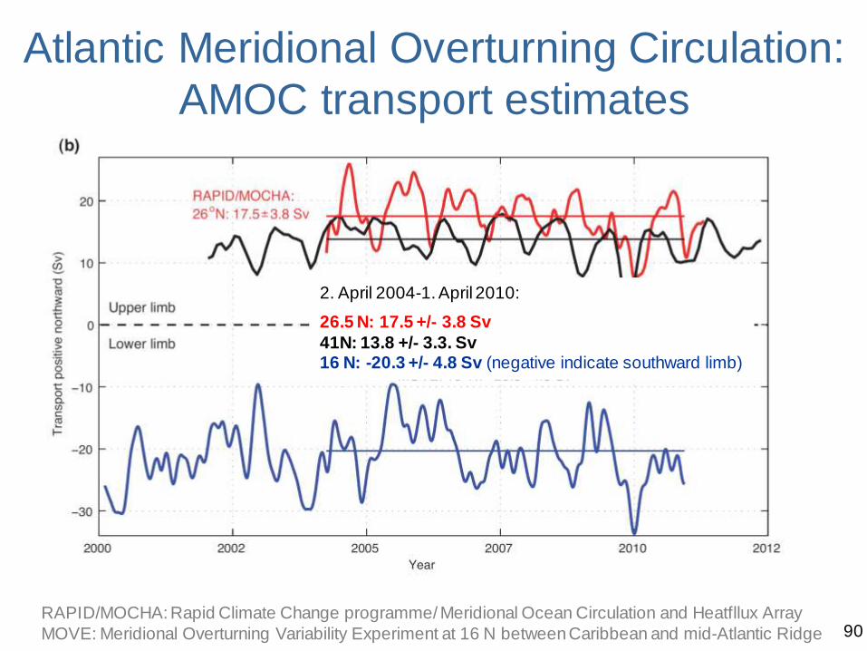
90 RAPID/MOCHA: Rapid Climate Change programme/ Meridional Ocean Circulation and Heatfllux Array

MOVE: Meridional Overturning Variability Experiment at 16 N between Caribbean and mid-Atlantic Ridge

2. April 2004-1. April 2010:

26.5 N: 17.5 +/- 3.8 Sv

41N: 13.8 +/- 3.3. Sv 16 N: -20.3 +/- 4.8 Sv (negative indicate southward limb)

Atlantic Meridional Overturning Circulation:

AMOC transport estimates

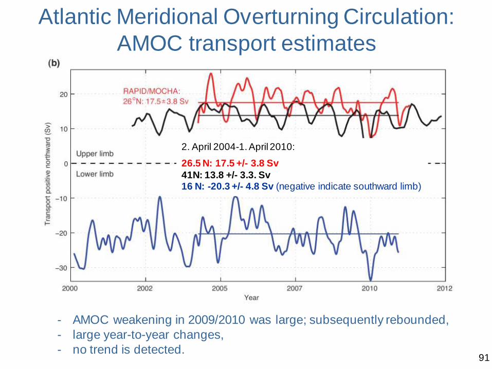
91

- AMOC weakening in 2009/2010 was large; subsequently rebounded,

- large year-to-year changes,

- no trend is detected.

2. April 2004-1. April 2010:

26.5 N: 17.5 +/- 3.8 Sv

41N: 13.8 +/- 3.3. Sv 16 N: -20.3 +/- 4.8 Sv (negative indicate southward limb)

3.6 Conclusions: Changes in Ocean Circulation

• Recent observations have strengthened evidence for variability in

major ocean circulation systems on time scales from years to decades.

• It is very likely that the subtropical gyres in the North Pacific and

South Pacific have expanded and strengthened since 1993. It is

about as likely as not that this is linked to decadal variability in wind

forcing rather than being part of a longer-term trend.

• Based on measurements of the full Atlantic Meridional Overturning

Circulation and its individual components at various latitudes and

different time periods, there is no evidence of a long-term trend.

• There is also no evidence for trends in the transports of the

Indonesian Throughflow, the Antarctic Circumpolar Current (ACC),

or between the Atlantic Ocean and Nordic Seas.

• However, there is medium confidence that the ACC shifted south

between 1950 and 2010, at a rate equivalent to about 1°of latitude

in 40 years. 92

gef4400 “the earth system” - uio.no filemode and thermocline waters in red to bottom waters in...

Documents