gated community premiums and amenity dif...
TRANSCRIPT
J R E R u V o l . 3 7 u N o . 3 – 2 0 1 5
G a t e d C o m m u n i t y P r e m i u m s a n d A m e n i t y
D i f f e r e n t i a l s i n R e s i d e n t i a l S u b d i v i s i o n s
A u t h o r s Evgeny L. Radetskiy, Ronald W. Spahr, and
Mark A. Sunderman
A b s t r a c t We use hedonic models to examine price differences betweensingle-family homes in gated communities and a matched samplein non-gated communities in Shelby County, Tennessee.Controlling for idiosyncratic attributes, we find that homes ingated communities carry significant price premiums relative tosimilar homes in non-gated communities. Price premiums arehighest for medium-size gated communities. Premiums were alsoevident in higher priced gated communities before 2008 butvanished after the financial crisis. Gated communities offerhomeowners additional attributes but usually have higherinfrastructure and service costs. Thus price premiums result fromnet gated community benefits.
Gated communities are residential developments characterized by physical securitymeasures such as gates, walls, guards, and closed-circuit television cameras. Acommon feature is a perimeter wall/fence enclosing the entire development andvehicular access is usually restricted by a gate, controlled by access cards, PINcodes, remote controls or security personnel. Security within the community isprovided by various means, including 24-hour security guard patrols, ‘‘back-to-base’’ alarm systems and panic buttons, closed-circuit television cameras, guarddogs, electric fencing, spikes, and other forms of anti-intruder perimeter controlsystems.
Gated communities and residents’ associations are not just an Americanphenomenon. Gated communities have experienced growth in Argentina, Brazil,Chile, China, France, Russia, Serbia, and the United Kingdom;1 however,approximately 65,700,000 Americans reside in association-governed communities,including homeowners associations, gated communities, planned unitdevelopments, condominiums, and cooperatives.2 According to the AmericanHousing Survey (2009), there were 10,759,000 units located in communitieswhose access is secured with walls, gates or fences.3 In the United States, gatedcommunities have grown to the point where such developments now account forroughly 11% of all new housing (e.g., McKenzie, 1994; Blakely and Snyder, 1997;Blandy, Lister, Atkinson, and Flint, 2003; Atkinson and Blandy, 2005). It is

4 0 6 u R a d e t s k i y , S p a h r , a n d S u n d e r m a n
generally concluded that gated communities transpire out of fear, anxiety, andinsecurity of urban inhabitants. Other factors may include economic restructuring,global terrorism, crime, immigration, the privatization of public services, and aperceived undermining of democratic processes. Thus, to protect themselves fromthese perceived risks and uncertainties, homeowners may desire to create a bufferbetween themselves and their families and society at large.
We temporally examine the existence of price premiums for a sample of single-family homes in private, gated residential communities relative to values incomparable non-gated communities in Memphis and Shelby County, Tennessee.Each gated community is matched with a control sample of similar non-gatedproperties in geographically adjacent or close proximity communities. Non-gatedcommunities are also matched with gated communities based on average saleprice, total living area, total lot area, and age.
We obtain housing sales data from the Shelby County, Tennessee Assessor’s Officefor a sample period from 2000 through 2012, and apply hedonic modeling similarto that used in a number of studies including Asabere and Huffman (1991),Sunderman and Birch (2002), Sunderman and Spahr (2004, 2006), and Spahrand Sunderman (2009), and consider modifications suggested by Sirmans,MacPherson, and Zietz (2005).
Our findings may be applicable to other locations in the U.S. because of the ethnic,racial, and economic diversity of our sample. Our results are consistent with thoseobtained by Helsley and Strange (1999) and LaCour-Little and Malpezzi (2009).
We add to the literature in a number of ways. We apply hedonic valuation modelsto control for and value unique, distinctive aspects of individual property- andcommunity-specific amenities such as clubhouses, community swimming pools,tennis courts, guard buildings, etc., associated with both gated and non-gatedcommunities. While controlling for unique property attributes, we find that single-family homes in gated communities generally command statistically significanthigher prices relative to comparable non-gated communities. Also, we study theinfluence of relative gated community size on price premiums, finding that sizeimpacts average property values. Medium-size gated communities appear to carrythe highest price premium as compared to smaller and larger gated communities.We also find that more affluent (higher priced) gated communities commandstatistically significant, higher gate premiums than do less affluent (lower priced)gated communities. Gates and access controls appear to be more highly valuedby buyers in more affluent communities.
Additionally, our data period permits us to consider most of the housing cyclefrom 2000 to 2012, allowing us to examine whether gated communities sustainedprice premiums before and subsequent to the 2008–2009 subprime crisis. Also,we refine this analysis, using median sale prices for each year for each communityand the median of the median prices, to classify each gated community and itsmatching non-gated community into either the higher priced or lower priced

G a t e d C o m m u n i t y P r e m i u m s u 4 0 7
J R E R u V o l . 3 7 u N o . 3 – 2 0 1 5
group. We find that higher priced and lower priced gated communities retainedvalues differently before and after the financial crisis. Prior to the crisis, higherpriced gated communities carried significant price premiums over comparable non-gated communities, whereas evidence of price premiums is mixed for lower pricedgated communities. Subsequent to the crisis, however, we find that neither higherpriced nor lower priced gated communities command statistically significant pricepremiums over their matching non-gated counterparts.
In Section 2, we review of the literature. We present the data and methodologyin Section 3. We discuss the results and robustness tests in Section 4. Concludingremarks are given in Section 5.
u R e v i e w o f t h e L i t e r a t u r e
Given the relatively recent proliferation of gated communities in Shelby County,Tennessee, as well as in the U.S., we study the motivation behind both the increasein gated communities and whether there are significant economic componentsassociated with them. LaCour-Little and Malpezzi (2009) find that price premiumsassociated with properties in gated communities result from net tradeoffs amongpositive benefits and higher infrastructure costs. Helsey and Strange (1999), usinga microeconomic approach, attribute price premiums to reduced crime levels ingated communities relative to non-gated communities. In addition to safetyconsiderations, we use hedonic modeling (a valuation/pricing approach) toquantify net specific tradeoffs between identified benefits and costs as justificationfor price premiums.
Homeowners within gated communities typically own undivided interests in streetsand sidewalks in addition to fee simple land ownership on which their homes sit(LaCour-Little and Malpezzi, 2009). Homeowners associations generally managethe streets, sidewalks, and common areas, where regular and occasionalassessments may be imposed on property owners to fund maintenance. Ascompensation for added costs, residents of gated communities gain control of thestreets, thereby restricting access, reducing traffic, noise, and possibly crime. Thus,despite the additional costs associated with living in gated communities, thebenefits outweigh the additional ownership costs if value premiums exist.
Bible and Hsieh (2001) and LaCour-Little and Malpezzi (2009) observe securityas the most common cited reason influencing gated community price premiums;however, they also posit the existence of a number of other reasons for potentialpremiums.4 The perception that a gate reduces crime within the community is bestexplained by the concept of ‘‘defensible space’’ credited to Newman (1973, 1980,1992, 1995). Newman initially studies the incidence of crime in gatedcommunities located very near a high crime housing project in St. Louis and findsthat they experienced lower crime and full occupancy throughout the study period.Based on data from the American Housing Survey for fee-paying gated and non-gated neighborhoods, Chapman and Lombard (2006) find that neighborhoodresident satisfaction levels strongly depend on the perception of a lack of crime.
4 0 8 u R a d e t s k i y , S p a h r , a n d S u n d e r m a n
Hardin and Cheng (2003) investigate the impact of security and crime protectionafforded by gated access and look at the effect on garden apartment rents. Theyfind that rents are positively related to the presence of gated access constraints.Thus, not only homeowners, but also renters are willing to pay for additionalsecurity provided by a gate.
The value of gated property security extends beyond residential properties.Benjamin, Chinloy, and Hardin (2007) find that gated commercial properties yieldrent premiums as compared to non-gated commercial properties when controllingfor other physical characteristics and ownership-management types.
Wilson-Doenges (2000) studies gated versus non-gated communities in both highincome and low income neighborhoods in Southern California. As may beexpected, personal safety and community safety perceptions per capita are higherin the high income gated versus non-gated community. However, perceptions ofdifferences in crime rates between gated and non-gated communities are notstatistically significant in both high and low income communities.
Other factors also may affect gated community price premiums. For example, itis important to consider the impact of additional conveniences such a communitymay offer. Researchers have explored the effects of amenities, other than security,on community real estate values. Benefield (2009) studies packages of amenityofferings and their impact on property values in neighborhoods. He finds that someamenity packages positively influence property values.5 Contrary to his study, weconclude that other amenities found within gated communities negatively impactproperty values when also controlling for amenities associated with individualproperties, neighborhood size, and affluence. We attribute our finding of negativevalues for community amenities, such as neighborhood swimming pools, resultsfrom many individual properties duplicating the same amenities.
Regardless of gated community attributes, such as crime reduction, perception ofincreased security and other amenities, they have been the target of criticismsfrom academics, the media, and the wider community. These criticisms generallyfocus on the potential divisions within the community caused by the gatedcommunities. For example, Kennedy (1995) argues that residential associations(including gated neighborhoods) carry negative externalities for nonmembers inthe form of discrimination on race and class, limiting a right to travel on privatestreets (raising a possibility of harassment by security guards or police), and evena reduction in free speech rights. If, however, gated communities address the fearsand anxieties of homeowners by enhancing personal safety, the security of materialgoods, as well as protecting homes from unwanted intrusions, the value of theseattributes may outweigh the negative externalities and additional costs of suchcommunities, thereby creating a price premium. Further, the physical design andcontrol of gated neighborhoods may assist in fostering a sense of community andcommon purpose among residents (McKenzie, 1994; Lang and Danielsen, 1997).
The valuation of properties within gated communities is the subject of severalstudies. Most notably, Bible and Hsieh (2001) use hedonic pricing and find that

G a t e d C o m m u n i t y P r e m i u m s u 4 0 9
J R E R u V o l . 3 7 u N o . 3 – 2 0 1 5
gated community properties have price premiums. We refine Bible and Hsieh’smodel by controlling for additional features possibly available within gatedcommunities, such as clubhouses, community swimming pools, tennis courts,basketball courts, and small lakes or ponds.
LaCour-Little and Malpezzi (2009) further support value premiums for gatedcommunities while also controlling for other neighborhood attributes, such as thepresence of homeowners associations6 and privately owned streets. They find thatprice premiums, relative to their non-gated counterparts, range from 7% to 24%for gated neighborhoods in Southern California and 13% for gated neighborhoodsin St. Louis.
Pompe (2008), also using a hedonic approach, finds that beach locations are morehighly valued by residents of gated communities, as compared to similar non-gated communities. Contrary to our findings, Le Goix (2007), using 1990–2000data for metropolitan Los Angeles, California, constructs an index of discontinuityfinding that large, high-end gated communities maintained price premiums andjustify higher governance/maintenance costs over time, whereas less affluent gatedcommunities (‘‘middle class’’ gated communities) did not. Also, contrary to ourfinding, Le Goix and Vasselinov (2013), using data through 2008, which may notmeasure the full impact of the housing crisis, conclude that properties within gatedcommunities are more immune to an unexpected decrease in property valuesduring periods of financial distress as compared to non-gated properties. However,they found some evidence that price premiums in gated communities had negativeprice effects on nearby financially distressed non-gated community properties.They posit that the presence of gated communities within a financially stressedneighborhood may destabilize the prices of nearby non-gated communities. Wefind that both higher priced and lower priced gated communities failed to sustainprice premiums subsequent to the recent financial crisis.
u D a t a a n d M e t h o d o l o g y
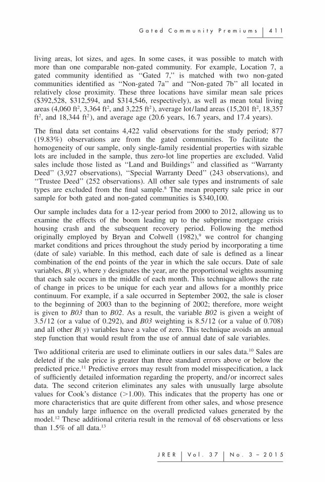
Sales data, including descriptions of single-family residential properties in ShelbyCounty from January, 2000 through December, 2012, are from the 2013 CertifiedAssessment Roll for Shelby County, Tennessee. The sample includes 11 fullygated communities from several different areas of Shelby County.7 Data alsoinclude sales from 16 comparable communities, where each gated community ismatched with non-gated communities with very similar locations and propertycharacteristics. The communities deemed to be comparable to gated communitiesare assessed based on location (proximity to a gated community), total living area(measured in square feet), sale price, and age of the property. The mean sale pricein the lowest priced gated community is $185,763 and the mean sale price in thehighest priced gated community is $1,315,490.
Exhibit 1 contains the summary statistics. Each gated community is matched withat least one comparable non-gated community based on similar sale prices, total
4 1 0 u R a d e t s k i y , S p a h r , a n d S u n d e r m a n
Exhibi t 1 u Descriptive Statistics for Sample Property Sales
Community Sale Price Total Living Area (ft 2 ) Land Area (ft 2 ) Age of House (Years)
Location 1 (loc1)Gated 1 $229,470 2,860.0 9,287.3 1.8Non-gated 1a $205,297 2,888.6 11,216.5 3.4Non-gated 1b $293,632 3,668.5 17,734.6 3.1
Location 2 (loc2)Gated 2 $311,738 3,434.8 12,685.2 13.1Non-gated 2 $260,261 2,975.5 16,058.9 13.2Gated 2.1 $382,673 3,575.9 13,085 6.7Non-gated 2.1 $348,976 3,969.6 19,244.2 18.7
Location 3 (loc3)Gated 3 $476,075 4,087.4 13,984.4 4.1Non-gated 3a $401,675 3,930.3 19,456.2 8.7Non-gated 3b $501,625 4,326.3 19,349.4 2.7
Location 4 (loc4)Gated 4 $185,763 2,301.3 7,743.1 9.1Non-gated 4a $210,899 2,839.9 10,594.3 8.6Non-gated 4b $172,047 2,280.1 10,973.5 6.9
Location 5 (loc5)Gated 5 $481,832 3,880.9 15,668.2 1.5Non-gated 5 $382,947 3,678.4 20,995.5 2.0
Location 6 (loc6)Gated 6 $342,826 3,678.3 23,189.1 2.4Non-gated 6 $251,824 3,300.3 20,254.2 32.6
Location 7 (loc7)Gated 7 $392,528 4,060.7 15,201.5 20.6Non-gated 7a $312,594 3,364.9 18,357.3 16.7Non-gated 7b $314,546 3,255.4 18,344.3 17.4
Location 8 (loc8)Gated 8 $494,872 4,930.7 37,979.0 9.8Non-gated 8 $284,253 3,708.0 24,462.4 17.3
Location 9 (loc9)Gated 9 $240,399 2,350.4 7,531.6 17.8Non-gated 9a $362,888 3,457.0 14,194.7 9.9Non-gated 9b $296,223 2,907.7 10,494.3 10.0
Location 10 (loc10)Gated 10 $1,315,490 6,406.1 20,883.7 4.5Non-gated 10 $675,169 5,132.9 31,908.0 22.1
Notes: Values represent means for each neighborhood. Gated communities Gated 2 and Gated2.1 and respective comparable communities are located in the same proximate location. Age ofeach house was calculated as the difference between the year of sale and the year house wasbuilt. Gated community names are provided by request.
G a t e d C o m m u n i t y P r e m i u m s u 4 1 1
J R E R u V o l . 3 7 u N o . 3 – 2 0 1 5
living areas, lot sizes, and ages. In some cases, it was possible to match withmore than one comparable non-gated community. For example, Location 7, agated community identified as ‘‘Gated 7,’’ is matched with two non-gatedcommunities identified as ‘‘Non-gated 7a’’ and ‘‘Non-gated 7b’’ all located inrelatively close proximity. These three locations have similar mean sale prices($392,528, $312,594, and $314,546, respectively), as well as mean total livingareas (4,060 ft2, 3,364 ft2, and 3,225 ft2), average lot/ land areas (15,201 ft2, 18,357ft2, and 18,344 ft2), and average age (20.6 years, 16.7 years, and 17.4 years).
The final data set contains 4,422 valid observations for the study period; 877(19.83%) observations are from the gated communities. To facilitate thehomogeneity of our sample, only single-family residential properties with sizablelots are included in the sample, thus zero-lot line properties are excluded. Validsales include those listed as ‘‘Land and Buildings’’ and classified as ‘‘WarrantyDeed’’ (3,927 observations), ‘‘Special Warranty Deed’’ (243 observations), and‘‘Trustee Deed’’ (252 observations). All other sale types and instruments of saletypes are excluded from the final sample.8 The mean property sale price in oursample for both gated and non-gated communities is $340,100.
Our sample includes data for a 12-year period from 2000 to 2012, allowing us toexamine the effects of the boom leading up to the subprime mortgage crisishousing crash and the subsequent recovery period. Following the methodoriginally employed by Bryan and Colwell (1982),9 we control for changingmarket conditions and prices throughout the study period by incorporating a time(date of sale) variable. In this method, each date of sale is defined as a linearcombination of the end points of the year in which the sale occurs. Date of salevariables, B( y), where y designates the year, are the proportional weights assumingthat each sale occurs in the middle of each month. This technique allows the rateof change in prices to be unique for each year and allows for a monthly pricecontinuum. For example, if a sale occurred in September 2002, the sale is closerto the beginning of 2003 than to the beginning of 2002; therefore, more weightis given to B03 than to B02. As a result, the variable B02 is given a weight of3.5/12 (or a value of 0.292), and B03 weighting is 8.5/12 (or a value of 0.708)and all other B( y) variables have a value of zero. This technique avoids an annualstep function that would result from the use of annual date of sale variables.
Two additional criteria are used to eliminate outliers in our sales data.10 Sales aredeleted if the sale price is greater than three standard errors above or below thepredicted price.11 Predictive errors may result from model misspecification, a lackof sufficiently detailed information regarding the property, and/or incorrect salesdata. The second criterion eliminates any sales with unusually large absolutevalues for Cook’s distance (.1.00). This indicates that the property has one ormore characteristics that are quite different from other sales, and whose presencehas an unduly large influence on the overall predicted values generated by themodel.12 These additional criteria result in the removal of 68 observations or lessthan 1.5% of all data.13

4 1 2 u R a d e t s k i y , S p a h r , a n d S u n d e r m a n
The data set includes numerous property characteristics for each property saleused in the analysis. The variables in the models are defined in Exhibit 2 andselected summary statistics for these variables are shown in Exhibit 3.
Sales price is the dependent or predicted variable in each of our hedonic models.It is assumed that sale price is a good estimate of true market value and may beexplained/predicted by selected independent-explanatory variables. A number ofexplanatory variables are generally employed when multiple regression (hedonicmodeling) is used to estimate improved residential property values. Variablesinclude style of building, wall construction, size, grade of construction,14 age, andother property characteristics. Additionally, we employ variables to control forother gated community amenities that may affect property values, such as thepresence of a clubhouse, public swimming pool, tennis court, basketball court,pond, and guard building.15 Each gated community and its matched comparablenon-gated community(ies) are assigned a unique location variable, LOCx . Thesedummy variables control for each of the 10 locations. Our general least squareslinear regression model is:
Price 5 a 1 b*Gate 1 c*X 1 d*Date of Salei,t i,t i,j,t i
1 e*Location 1 « , (1)i i,t
where Pricei,t is the sale price of the property i at time t. Gatei,t is a dichotomous(dummy) variable indicating if the community of the sale is gated (1) or not (0).Xi, j,t represents a vector of property attributes/characteristics for property i,attribute j in period t (age, size, number of bathrooms, etc.). Date of Salei
represents linear combinations of the end points of the year in which sale i occurs,and Locationi indicates each property’s location.
u E m p i r i c a l R e s u l t s f o r H e d o n i c P r i c i n g M o d e l
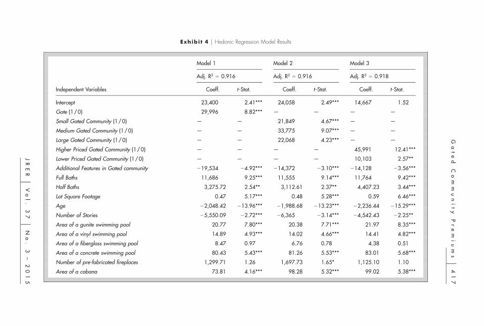
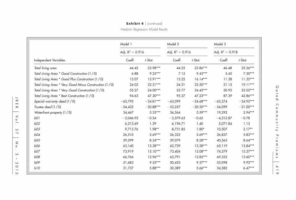
Referring to Exhibit 4, Model 1 represents a good fit with an adjusted R2 of 0.916.Variance inflation factors (VIFs) are run for all variables and are deemedacceptable (VIF , 10.0),16 reducing multicollinearity concerns among independentvariables. A dummy variable controlling for the presence of a gate measures itseconomic impact on property and amenity values. Empirical results indicate thatthe average sale price premium for properties located in gated communities is$29,996 relative to comparable properties in non-gated communities. The pricepremium is statistically significant at the 99% confidence level.17
As is the case with gated communities throughout the country, the residents ofgated communities in our study are responsible for upkeep of roads, drainage, andother maintenance that normally would be covered by the municipality for non-gated communities, thus the $29,996 increase in value is the net increase inproperty values above additional associated costs.

G a t e d C o m m u n i t y P r e m i u m s u 4 1 3
J R E R u V o l . 3 7 u N o . 3 – 2 0 1 5
Exhibi t 2 u Independent Variables
Variable Name Description
Gate Dummy Variable: Equals 1 if community is gated; 0otherwise
Small Gated Community Dummy Variable: Equals 1 if gated community hasbetween 38 and 42 houses; 0 otherwise
Medium Gated Community Dummy Variable: Equals 1 if gated community hasbetween 65 and 106 houses; 0 otherwise
Large Gated Community Dummy Variable: Equals 1 if gated community hasbetween 126 and 181 houses; 0 otherwise
Higher Priced Gated Community Dummy Variable: Equals to 1 if gated community is‘‘higher priced’’; 0 otherwise
Lower Priced Gated Community Dummy Variable: Equals to 1 if gated community is‘‘lower priced’’; 0 otherwise
Additional Features in Gated community Dummy Variable: Equals 1 if gated community haseither clubhouse, swimming pool, cabana, tenniscourt, basketball court, pond, or guard building; 0otherwise
Full Baths Number of full baths
Half Baths Number of half baths
Lot Square Footage Total area of the property (ft 2)
Age Age of the property; it is calculated as a differencebetween ‘‘Year of Sale’’ and ‘‘Year Built’’
Number of Stories Number of stories a property has
Area of a gunite swimming pool Area of a gunite swimming pool (ft 2)
Area of a vinyl swimming pool Area of a vinyl swimming pool (ft 2)
Area of a fiberglass swimming pool Area of a fiberglass swimming pool (ft 2)
Area of a concrete swimming pool Area of a concrete swimming pool (ft 2)
Number of pre-fabricated fireplaces Number of pre-fabricated fireplaces a property has
Area of a cabana Area of a cabana (ft 2)
Crawl space Equals 1 if property has a crawl space; 0 otherwise
Area of carport Area of a carport (ft 2)
Area of garage Area of a garage (ft 2)
Area of a stone patio Area of a stone patio (ft 2)
Golf Dummy Variable: Equals 1 if property has an accessto the golf course; 0 otherwise
Stucco exterior wall Dummy Variable: Equals 1 if exterior wall material isstucco; 0 otherwise
Vinyl exterior wall Dummy Variable: Equals 1 if exterior wall material isvinyl; 0 otherwise
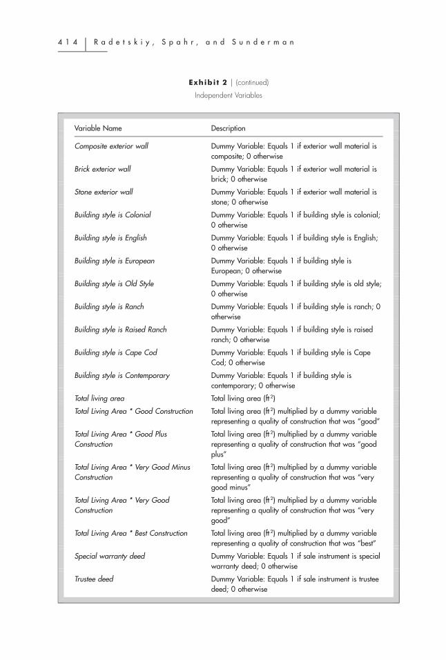
4 1 4 u R a d e t s k i y , S p a h r , a n d S u n d e r m a n
Exhibi t 2 u (continued)
Independent Variables
Variable Name Description
Composite exterior wall Dummy Variable: Equals 1 if exterior wall material iscomposite; 0 otherwise
Brick exterior wall Dummy Variable: Equals 1 if exterior wall material isbrick; 0 otherwise
Stone exterior wall Dummy Variable: Equals 1 if exterior wall material isstone; 0 otherwise
Building style is Colonial Dummy Variable: Equals 1 if building style is colonial;0 otherwise
Building style is English Dummy Variable: Equals 1 if building style is English;0 otherwise
Building style is European Dummy Variable: Equals 1 if building style isEuropean; 0 otherwise
Building style is Old Style Dummy Variable: Equals 1 if building style is old style;0 otherwise
Building style is Ranch Dummy Variable: Equals 1 if building style is ranch; 0otherwise
Building style is Raised Ranch Dummy Variable: Equals 1 if building style is raisedranch; 0 otherwise
Building style is Cape Cod Dummy Variable: Equals 1 if building style is CapeCod; 0 otherwise
Building style is Contemporary Dummy Variable: Equals 1 if building style iscontemporary; 0 otherwise
Total living area Total living area (ft 2)
Total Living Area * Good Construction Total living area (ft 2) multiplied by a dummy variablerepresenting a quality of construction that was ‘‘good’’
Total Living Area * Good PlusConstruction
Total living area (ft 2) multiplied by a dummy variablerepresenting a quality of construction that was ‘‘goodplus’’
Total Living Area * Very Good MinusConstruction
Total living area (ft 2) multiplied by a dummy variablerepresenting a quality of construction that was ‘‘verygood minus’’
Total Living Area * Very GoodConstruction
Total living area (ft 2) multiplied by a dummy variablerepresenting a quality of construction that was ‘‘verygood’’
Total Living Area * Best Construction Total living area (ft 2) multiplied by a dummy variablerepresenting a quality of construction that was ‘‘best’’
Special warranty deed Dummy Variable: Equals 1 if sale instrument is specialwarranty deed; 0 otherwise
Trustee deed Dummy Variable: Equals 1 if sale instrument is trusteedeed; 0 otherwise
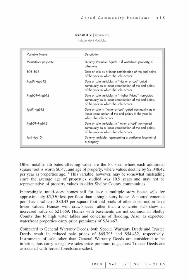
G a t e d C o m m u n i t y P r e m i u m s u 4 1 5
J R E R u V o l . 3 7 u N o . 3 – 2 0 1 5
Exhibi t 2 u (continued)
Independent Variables
Variable Name Description
Waterfront property Dummy Variable: Equals 1 if waterfront property; 0otherwise
b01–b13 Date of sale as a linear combination of the end pointsof the year in which the sale occurs
hgb01–hgb12 Date of sale variables in ‘‘higher priced’’ gatedcommunity as a linear combination of the end pointsof the year in which the sale occurs
hngb01–hngb12 Date of sale variables in ‘‘Higher Priced’’ non-gatedcommunity as a linear combination of the end pointsof the year in which the sale occurs
lgb01–lgb12 Date of sale in ‘‘lower priced’’ gated community as alinear combination of the end points of the year inwhich the sale occurs
lngb01–lngb12 Date of sale variables in ‘‘lower priced’’ non-gatedcommunity as a linear combination of the end pointsof the year in which the sale occurs
loc1–loc10 Dummy variables representing a particular location ofa property
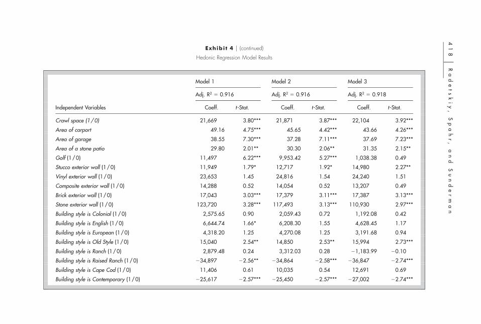
Other notable attributes affecting value are the lot size, where each additionalsquare foot is worth $0.47, and age of property, where values decline by $2,048.42per year as properties age.18 This variable, however, may be somewhat misleadingsince the average age of properties studied was 10.9 years and may not berepresentative of property values in older Shelby County communities.
Interestingly, multi-story homes sell for less; a multiple story house sells forapproximately $5,550 less per floor than a single-story house. A poured concretepool has a value of $80.43 per square foot and pools of other construction havelower values. Houses with crawlspaces rather than a concrete slab show anincreased value of $21,669. Homes with basements are not common in ShelbyCounty due to high water tables and concerns of flooding. Also, as expected,waterfront properties carry price premiums of $34,467.
Compared to General Warranty Deeds, both Special Warranty Deeds and TrusteeDeeds result in reduced sale prices of $65,795 and $54,432, respectively.Instruments of sale other than General Warranty Deeds are considered to beinferior, thus carry a negative sales price premium (e.g., most Trustee Deeds areassociated with forced foreclosure sales).

4 1 6 u R a d e t s k i y , S p a h r , a n d S u n d e r m a n
Exhibi t 3 u Descriptive Statistics of the Full Sample
Variable N Mean Median Std. Dev. Min. Max.
Price (USD) 4,422 340,100 322,000 152,287 21,000 2,403,300
Land Area (ft 2) 4,422 17,382 15,973 9,836 5,750 328,372
Age (Years) 4,422 10.9 9.0 9.2 1 62
Total Living Area (ft 2) 4,422 3,544 3,465 847 1,675 10,860
Variable N% of TotalSample
Number of Sales in Gated CommunitiesProperties in GatedCommunities
877 19.83%
Number of Total Sales (Gated and Non-gated) by LocationLocation 1 533 12.05%Location 2 472 10.67%Location 3 1,100 24.86%Location 4 501 11.33%Location 5 412 9.32%Location 6 289 6.54%Location 7 747 16.89%Location 8 169 3.82%Location 9 94 2.13%Location 10 105 2.38%
Properties in communities, whether gated or non-gated, with a golf course sell for$11,497 more than for communities without a golf course. These findings areconsistent with Do and Grudnitski (1995), Grudnitski (2003), and Shultz andSchmitz (2009).19
Each square foot of living area is worth $44.42 for a house with average qualityof construction. Unsurprisingly, the value of each additional square foot of livingarea increases with higher quality construction. The grade of construction variesfrom average (the base variable on which each higher quality of constructionvariable is compared) to good, good plus, very good minus, very good, and best.As expected, a ‘‘good’’ construction quality house sells for an additional $6.88per square foot when compared to a house with average quality of construction.Values for good plus, very good minus, very good, and best are $15.07, $24.02,$55.27, and $94.63, respectively. As a result, a home built with the best qualityof construction would be worth $139.05 per square foot.
Annual date of sale variables, B( y), represent market values relative to the baseyear, 2000. Since Shelby County did not experience the significant run up inmarket values prior to the recent financial crisis that were observed in other parts
Ga
te
dC
om
mu
ni
ty
Pr
em
iu
ms
u4
17
JR
ER
uV
ol
.3
7u
No
.3
–2
01
5
Exhibi t 4 u Hedonic Regression Model Results
Model 1 Model 2 Model 3
Adj. R25 0.916 Adj. R2
5 0.916 Adj. R25 0.918
Independent Variables Coeff. t -Stat. Coeff. t -Stat. Coeff. t -Stat.
Intercept 23,400 2.41*** 24,058 2.49*** 14,667 1.52
Gate (1/0) 29,996 8.82*** — — — —
Small Gated Community (1/0) — — 21,849 4.67*** — —
Medium Gated Community (1/0) — — 33,775 9.07*** — —
Large Gated Community (1/0) — — 22,068 4.23*** — —
Higher Priced Gated Community (1/0) — — — — 45,991 12.41***
Lower Priced Gated Community (1/0) — — — — 10,103 2.57**
Additional Features in Gated community 219,534 24.92*** 214,372 23.10*** 214,128 23.56***
Full Baths 11,686 9.25*** 11,555 9.14*** 11,764 9.42***
Half Baths 3,275.72 2.54** 3,112.61 2.37** 4,407.23 3.44***
Lot Square Footage 0.47 5.17*** 0.48 5.28*** 0.59 6.46***
Age 22,048.42 213.96*** 21,988.68 213.23*** 22,236.44 215.29***
Number of Stories 25,550.09 22.72*** 26,365 23.14*** 24,542.43 22.25**
Area of a gunite swimming pool 20.77 7.80*** 20.38 7.71*** 21.97 8.35***
Area of a vinyl swimming pool 14.89 4.93*** 14.02 4.66*** 14.41 4.82***
Area of a fiberglass swimming pool 8.47 0.97 6.76 0.78 4.38 0.51
Area of a concrete swimming pool 80.43 5.43*** 81.26 5.53*** 83.01 5.68***
Number of pre-fabricated fireplaces 1,299.71 1.26 1,697.73 1.65* 1,125.10 1.10
Area of a cabana 73.81 4.16*** 98.28 5.32*** 99.02 5.38***
41
8u
Ra
de
ts
ki
y,
Sp
ah
r,
an
dS
un
de
rm
an
Exhibi t 4 u (continued)
Hedonic Regression Model Results
Model 1 Model 2 Model 3
Adj. R25 0.916 Adj. R2
5 0.916 Adj. R25 0.918
Independent Variables Coeff. t -Stat. Coeff. t -Stat. Coeff. t -Stat.
Crawl space (1/0) 21,669 3.80*** 21,871 3.87*** 22,104 3.92***
Area of carport 49.16 4.75*** 45.65 4.42*** 43.66 4.26***
Area of garage 38.55 7.30*** 37.28 7.11*** 37.69 7.23***
Area of a stone patio 29.80 2.01** 30.30 2.06** 31.35 2.15**
Golf (1/0) 11,497 6.22*** 9,953.42 5.27*** 1,038.38 0.49
Stucco exterior wall (1/0) 11,949 1.79* 12,717 1.92* 14,980 2.27**
Vinyl exterior wall (1/0) 23,653 1.45 24,816 1.54 24,240 1.51
Composite exterior wall (1/0) 14,288 0.52 14,054 0.52 13,207 0.49
Brick exterior wall (1/0) 17,043 3.03*** 17,379 3.11*** 17,387 3.13***
Stone exterior wall (1/0) 123,720 3.28*** 117,493 3.13*** 110,930 2.97***
Building style is Colonial (1/0) 2,575.65 0.90 2,059.43 0.72 1,192.08 0.42
Building style is English (1/0) 6,644.74 1.66* 6,208.30 1.55 4,628.45 1.17
Building style is European (1/0) 4,318.20 1.25 4,270.08 1.25 3,191.68 0.94
Building style is Old Style (1/0) 15,040 2.54** 14,850 2.53** 15,994 2.73***
Building style is Ranch (1/0) 2,879.48 0.24 3,312.03 0.28 21,183.99 20.10
Building style is Raised Ranch (1/0) 234,897 22.56** 234,864 22.58*** 236,847 22.74***
Building style is Cape Cod (1/0) 11,406 0.61 10,035 0.54 12,691 0.69
Building style is Contemporary (1/0) 225,617 22.57*** 225,450 22.57*** 227,002 22.74***
Ga
te
dC
om
mu
ni
ty
Pr
em
iu
ms
u4
19
JR
ER
uV
ol
.3
7u
No
.3
–2
01
5
Exhibi t 4 u (continued)
Hedonic Regression Model Results
Model 1 Model 2 Model 3
Adj. R25 0.916 Adj. R2
5 0.916 Adj. R25 0.918
Independent Variables Coeff. t -Stat. Coeff. t -Stat. Coeff. t -Stat.
Total living area 44.42 23.98*** 44.25 23.86*** 46.48 25.26***
Total Living Area * Good Construction (1/0) 6.88 9.25*** 7.12 9.43*** 5.45 7.30***
Total Living Area * Good Plus Construction (1/0) 15.07 15.91*** 15.25 16.14*** 11.38 11.35***
Total Living Area * Very Good Minus Construction (1/0) 24.02 22.21*** 24.31 22.50*** 21.15 19.11***
Total Living Area * Very Good Construction (1/0) 55.27 24.00*** 55.77 24.45*** 50.95 22.02***
Total Living Area * Best Construction (1/0) 94.63 47.30*** 95.37 47.23*** 87.39 42.86***
Special warranty deed (1/0) 265,795 224.81*** 265,099 224.68*** 265,374 224.95***
Trustee deed (1/0) 254,432 220.88*** 253,257 220.50*** 254,099 221.00***
Waterfront property (1/0) 34,467 5.33*** 36,564 5.59*** 19,292 2.94***
b01 23,046.92 20.54 23,579.63 20.65 24,312.87 20.78
b02 6,213.69 1.39 6,196.71 1.40 5,071.84 1.15
b03 9,713.76 1.98** 8,731.85 1.80* 10,507 2.17**
b04 26,510 5.69*** 26,322 5.69*** 26,837 5.83***
b05 39,599 8.34*** 39,079 8.28*** 40,563 8.64***
b06 63,140 13.28*** 62,729 13.28*** 65,119 13.84***
b07 73,919 15.10*** 73,404 15.08*** 74,379 15.37***
b08 66,766 12.96*** 65,791 12.85*** 69,352 13.60***
b09 51,683 9.55*** 50,455 9.37*** 53,098 9.92***
b10 31,737 5.88*** 30,389 5.66*** 34,582 6.47***

42
0u
Ra
de
ts
ki
y,
Sp
ah
r,
an
dS
un
de
rm
an
Exhibi t 4 u (continued)
Hedonic Regression Model Results
Model 1 Model 2 Model 3
Adj. R25 0.916 Adj. R2
5 0.916 Adj. R25 0.918
Independent Variables Coeff. t -Stat. Coeff. t -Stat. Coeff. t -Stat.
b11 34,485 6.25*** 33,459 6.09*** 36,518 6.69***
b12 32,915 5.96*** 31,862 5.79*** 34,698 6.35***
b13 41,989 6.60*** 41,792 6.60*** 45,435 7.22***
Loc1 240,849 210.00*** 240,169 29.84*** 233,563 28.17***
Loc2 41,397 10.59*** 43,813 10.78*** 48,591 12.33***
Loc3 55,413 14.49*** 56,731 14.84*** 66,452 16.82***
Loc4 226,763 25.79*** 223,901 25.07*** 213,712 22.87***
Loc5 22,485 5.20*** 24,813 5.66*** 29,532 6.80***
Loc6 36,175 7.67*** 37,899 7.50*** 43,363 9.18***
Loc7 53,354 14.53*** 54,910 14.89*** 56,082 15.40***
Loc9 63,025 11.48*** 65,163 10.86*** 73,832 13.31***
Loc10 177,958 26.39*** 174,029 25.94*** 188,667 27.80***
Notes: The dependent variable is the price of the property. Special Warranty Deeds and Trustee Deeds are compared to General Warranty Deeds; allconstruction quality variables are compared to average quality of construction; annual date of sale variables (b01–b13) are compared to the base year,2000; all siding types variables are compared to wood siding; all house styles are compared to a traditional house style; all locations are compared tolocation 8.*Significant at the 10% level.**Significant at the 5% level.***Significant at the 1% level.

G a t e d C o m m u n i t y P r e m i u m s u 4 2 1
J R E R u V o l . 3 7 u N o . 3 – 2 0 1 5
of the country, except for 2001, market prices showed price increases until 2007.However, because of the excess supply of houses on the market and the financialcrisis, values began declining from a peak in 2007 ($73,919 above the price in2000) to a value in 2010 of only $31,737 above 2000 prices. By the end of 2012,home prices had rebounded to $41,989 above 2000 prices. To further interpretthese results, previously we indicated that a sale in September 2002 would havea weighted value assigned to B02 of 0.292 and 0.708 to B03. Multiplying theseweights by the coefficients in Model 1 for B02 (6,213.69) and B03 (9,713.76),the weighted average is $8,691.74. This indicates, holding all else constant, ahouse selling in September of 2002 carries a price premium of $8,691.74 aboveone sold at the beginning of 2000 and a price appreciation of $2,478.05 since thebeginning of 2002. Price patterns may be seen in Exhibit 7.20
Also, we control for additional amenities provided for residents of gatedcommunities, including the presence of a clubhouse, community swimming pool,cabana, tennis courts, basketball courts, small ponds/lakes, and for the existenceof a guard building in addition to a gate. Generally, we find that these amenitiescarry highly significant negative values, where the presence of these amenitiesreduces sale prices by $19,534. Although, at least superficially, these features seemto have value, we posit that additional maintenance costs associated with theseamenities outweigh their benefits.
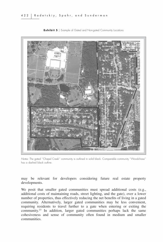
Location variables compare and control for price level differences among each ofthe other ten gated communities and comparable communities where ‘‘ChapelCreek,’’ the gated community, and its comparable ‘‘Woodchase’’ (Location 8) arethe base communities. See Exhibit 5 as an example of the location of ChapelCreek relative to it matched community Woodchase. Location variables range from2$40,849 to $177,958. For example, the variable for location 1 indicates a valueof $40,849 less than Chapel Creek, whereas the location 10 variable shows a pricelevel of $177,958 above Chapel Creek.
Other variables (attributes) may be observed in Exhibit 4.21 Overall, the hedonicmodel behaves as expected and not surprisingly, the variable of specific interestin this study, Gate, carries a significant impact on property values. Gatedproperties sell for $29,996 above similar parcels in non-gated communities.
In Model 2, we included three separate dummy variables to capture the impact ofrelative size (based on number of homes) for property values in gatedcommunities.22 Results, shown in Exhibit 4, represent a good fit where the adjustedR2 is 0.9160, VIF values are acceptable (VIF , 10.0), and no major changesrelative to Model 1 are observed.
The results for Model 2 show that medium-size communities carry the highestgate premium of $33,775; gate premiums for smaller and larger communities are$21,849 and $22,068, respectively. As in Model 1, additional amenities arenegatively statistically significant with an estimate of 2$14,372. The resultsindicate that there may be an optimal gated neighborhood size. This observation
4 2 2 u R a d e t s k i y , S p a h r , a n d S u n d e r m a n
Exhibi t 5 u Example of Gated and Non-gated Community Locations
Notes: The gated ‘‘Chapel Creek’’ community is outlined in solid black. Comparable community ‘‘Woodchase’’has a dashed black outline.
may be relevant for developers considering future real estate propertydevelopments.
We posit that smaller gated communities must spread additional costs (e.g.,additional costs of maintaining roads, street lighting, and the gate), over a lowernumber of properties, thus effectively reducing the net benefits of living in a gatedcommunity. Alternatively, larger gated communities may be less convenient,requiring residents to travel further to a gate when entering or exiting thecommunity.23 In addition, larger gated communities perhaps lack the samecohesiveness and sense of community often found in medium and smallercommunities.
G a t e d C o m m u n i t y P r e m i u m s u 4 2 3
J R E R u V o l . 3 7 u N o . 3 – 2 0 1 5
In Model 3, we study the impact of affluence on gated community values. Moreaffluent gated communities, because of higher real and personal property values,may assign higher values to gates and fences as compared with less affluent gatedcommunities. Gated communities in our sample are separated into ‘‘HigherPriced’’ and ‘‘Lower Priced’’ groups. To classify communities as higher or lowerpriced, we first determine a median sale price for each gated community over theentire 12-year study period. Then, we find a median of medians. If the mediansale price of a particular gated community is above the overall median of medians,the gated community is considered a higher priced community and vice versa forlower priced gated communities. Since we have 11 gated communities in oursample, the median of medians is equal to one of the gated community’s medianprice. For that gated community, we determine an average sale price, as well asthe median price. If the mean sale price is higher than the median sale price forthat community, then it is considered to belong to the higher priced group (andvice versa for the lower priced group).
In Model 3, each dummy variable (‘‘higher priced gated community’’ and ‘‘lower
priced gated community’’) captures the affluence effect on value of each gatedcommunity. The results are shown in Exhibit 4 (Model 3). Similar to Models 1and 2, Model 3 represents a good fit with an adjusted R2 of .9180. Varianceinflation factors (VIFs) are again tested in this model and it was found that allvariables are highly acceptable (all VIFs , 10.0). There are also no major changesin the overall model.
The results for Model 3 show that higher priced, more affluent gated communitiescarry higher premiums of $45,991; lower priced gated communities commandpremiums of $10,103. All relevant variables in Model 3 are statistically significant.
As in previous models, the additional features of gated communities arestatistically significant with an estimate of 2$14,128. For example, people residingin higher priced gated communities may assign little or no value to a communityswimming pool as they may already have pools on their properties (or tennis andbasketball courts). Also, the presence of additional community amenities appearto have negative values as homeowners may be unwilling to pay for expensesassociated with these benefits.
As an alternative to Model 3, we log-transform sale price while holding allindependent variables constant. The results show that higher priced communitygate premiums are 14.2% greater than values for their matched non-gatedcommunities; gate premiums for properties located in lower priced communitiesare only 3.8% higher than for their matched non-gated communities. These resultsprovide further evidence that more affluent gated communities command largerprice premiums.24
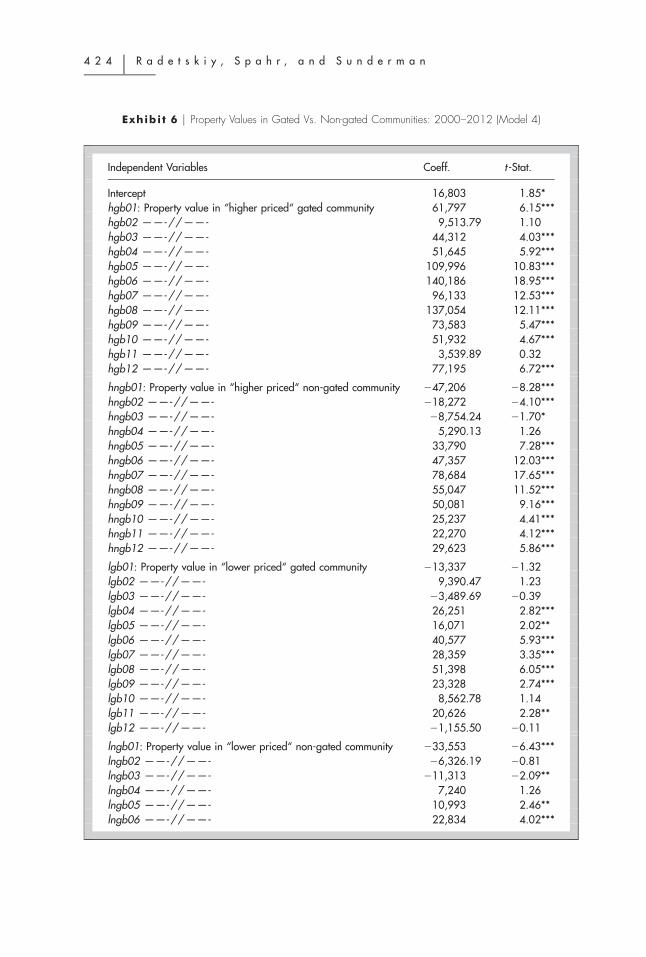
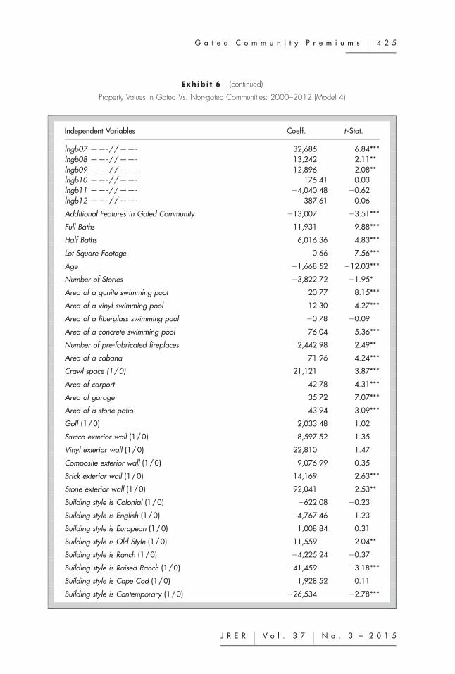
Value premiums for gated communities may vary across time and may bedependent on the housing market, thus we empirically test the sustainability ofgate premiums over different stages of an economic cycle. Model 4, shown inExhibit 6, measures relative price patterns temporally for higher and lower priced
4 2 4 u R a d e t s k i y , S p a h r , a n d S u n d e r m a n
Exhibi t 6 u Property Values in Gated Vs. Non-gated Communities: 2000–2012 (Model 4)
Independent Variables Coeff. t -Stat.
Intercept 16,803 1.85*hgb01: Property value in ‘‘higher priced‘‘ gated community 61,797 6.15***hgb02 ——-// ——- 9,513.79 1.10hgb03 ——-// ——- 44,312 4.03***hgb04 ——-// ——- 51,645 5.92***hgb05 ——-// ——- 109,996 10.83***hgb06 ——-// ——- 140,186 18.95***hgb07 ——-// ——- 96,133 12.53***hgb08 ——-// ——- 137,054 12.11***hgb09 ——-// ——- 73,583 5.47***hgb10 ——-// ——- 51,932 4.67***hgb11 ——-// ——- 3,539.89 0.32hgb12 ——-// ——- 77,195 6.72***
hngb01: Property value in ‘‘higher priced‘‘ non-gated community 247,206 28.28***hngb02 ——-// ——- 218,272 24.10***hngb03 ——-// ——- 28,754.24 21.70*hngb04 ——-// ——- 5,290.13 1.26hngb05 ——-// ——- 33,790 7.28***hngb06 ——-// ——- 47,357 12.03***hngb07 ——-// ——- 78,684 17.65***hngb08 ——-// ——- 55,047 11.52***hngb09 ——-// ——- 50,081 9.16***hngb10 ——-// ——- 25,237 4.41***hngb11 ——-// ——- 22,270 4.12***hngb12 ——-// ——- 29,623 5.86***
lgb01: Property value in ‘‘lower priced‘‘ gated community 213,337 21.32lgb02 ——-// ——- 9,390.47 1.23lgb03 ——-// ——- 23,489.69 20.39lgb04 ——-// ——- 26,251 2.82***lgb05 ——-// ——- 16,071 2.02**lgb06 ——-// ——- 40,577 5.93***lgb07 ——-// ——- 28,359 3.35***lgb08 ——-// ——- 51,398 6.05***lgb09 ——-// ——- 23,328 2.74***lgb10 ——-// ——- 8,562.78 1.14lgb11 ——-// ——- 20,626 2.28**lgb12 ——-// ——- 21,155.50 20.11
lngb01: Property value in ‘‘lower priced‘‘ non-gated community 233,553 26.43***lngb02 ——-// ——- 26,326.19 20.81lngb03 ——-// ——- 211,313 22.09**lngb04 ——-// ——- 7,240 1.26lngb05 ——-// ——- 10,993 2.46**lngb06 ——-// ——- 22,834 4.02***
G a t e d C o m m u n i t y P r e m i u m s u 4 2 5
J R E R u V o l . 3 7 u N o . 3 – 2 0 1 5
Exhibi t 6 u (continued)
Property Values in Gated Vs. Non-gated Communities: 2000–2012 (Model 4)
Independent Variables Coeff. t -Stat.
lngb07 ——-// ——- 32,685 6.84***lngb08 ——-// ——- 13,242 2.11**lngb09 ——-// ——- 12,896 2.08**lngb10 ——-// ——- 175.41 0.03lngb11 ——-// ——- 24,040.48 20.62lngb12 ——-// ——- 387.61 0.06
Additional Features in Gated Community 213,007 23.51***
Full Baths 11,931 9.88***
Half Baths 6,016.36 4.83***
Lot Square Footage 0.66 7.56***
Age 21,668.52 212.03***
Number of Stories 23,822.72 21.95*
Area of a gunite swimming pool 20.77 8.15***
Area of a vinyl swimming pool 12.30 4.27***
Area of a fiberglass swimming pool 20.78 20.09
Area of a concrete swimming pool 76.04 5.36***
Number of pre-fabricated fireplaces 2,442.98 2.49**
Area of a cabana 71.96 4.24***
Crawl space (1/0) 21,121 3.87***
Area of carport 42.78 4.31***
Area of garage 35.72 7.07***
Area of a stone patio 43.94 3.09***
Golf (1/0) 2,033.48 1.02
Stucco exterior wall (1/0) 8,597.52 1.35
Vinyl exterior wall (1/0) 22,810 1.47
Composite exterior wall (1/0) 9,076.99 0.35
Brick exterior wall (1/0) 14,169 2.63***
Stone exterior wall (1/0) 92,041 2.53**
Building style is Colonial (1/0) 2622.08 20.23
Building style is English (1/0) 4,767.46 1.23
Building style is European (1/0) 1,008.84 0.31
Building style is Old Style (1/0) 11,559 2.04**
Building style is Ranch (1/0) 24,225.24 20.37
Building style is Raised Ranch (1/0) 241,459 23.18***
Building style is Cape Cod (1/0) 1,928.52 0.11
Building style is Contemporary (1/0) 226,534 22.78***
4 2 6 u R a d e t s k i y , S p a h r , a n d S u n d e r m a n
Exhibi t 6 u (continued)
Property Values in Gated Vs. Non-gated Communities: 2000–2012 (Model 4)
Independent Variables Coeff. t -Stat.
Total living area 47.24 26.55***
Total Living Area * Good Construction (1/0) 4.72 6.55***
Total Living Area * Good Plus Construction (1/0) 11.69 12.27***
Total Living Area * Very Good Minus Construction (1/0) 20.71 19.51***
Total Living Area * Very Good Construction (1/0) 50.17 22.40***
Total Living Area * Best Construction (1/0) 86.92 43.99***
Special warranty deed (1/0) 256,781 222.01***
Trustee deed (1/0) 246,341 218.34***
Waterfront property (1/0) 28,153 4.31***
Loc1 214,935 23.16***
Loc2 68,100 15.86***
Loc3 72,980 19.29***
Loc4 5,856.38 1.12
Loc5 30,959 7.15***
Loc6 44,804 9.07***
Loc7 66,200 17.51***
Loc9 90,492 15.42***
Loc10 184,107 28.11***
Notes: The dependent variable is the price of the property in USD. Adjusted R25 0.924. Special
Warranty Deeds and Trustee Deeds are compared to General Warranty Deeds; all constructionquality variables are compared to average quality of construction; annual date of sale variablesare compared to the base year, 2000; all siding types variables are compared to wood siding; allhouse styles are compared to a traditional house style; all locations are compared to location 8.* Significant at the 10% level.** Significant at the 5% level.***Significant at the 1% level.
gated and non-gated communities. To measure this, we broke the date of salevariables, B( y), into higher priced gated, HGB( y), higher priced non-gated,HNGB( y), lower priced gated, LGB( y), and lower priced non-gated, LNGB( y).25
As in Model 3, we divide our sample into higher priced and lower pricedcommunities based on median sale prices except, in this situation, classificationof gated communities is completed annually. We then track each date of salevariable across time to determine price patterns for each community classification.This allows us to measure the effect of the housing crisis on property values andspecifically the temporal sustainability of gate premiums before, during, and after

G a t e d C o m m u n i t y P r e m i u m s u 4 2 7
J R E R u V o l . 3 7 u N o . 3 – 2 0 1 5
the housing crisis. These date values are shown in Exhibit 7, and for comparison,the date variables from Model 1 are also shown.
As previously discussed, gated communities carry price premiums only if theyhave a positive benefit/cost ratio. Exhibit 7 indicates that prior to the subprimecrisis (where the crisis period 2008–2009 is shaded), gated communities carriedsignificant price premiums over non-gated communities. However, beginning in2008, premiums for higher priced gated communities declined, and only in 2012did they appear to trend upward. Although, the lower priced gated communitiestypically show a premium over non-gated lower priced communities, gatepremiums were not as great as found in higher priced gated communities. Itappears that the subprime crisis impacted values for all communities in oursample; however, the decline in value was the largest for the higher priced gatedcommunities.
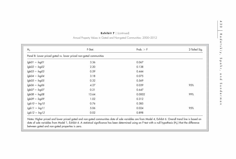
Date variable differences for each year between higher priced gated and higherpriced non-gated as well as between lower priced gated and lower priced non-gated communities are tested for statistical significance using an F-test with a nullhypothesis (H0) that the difference between gated and non-gated properties arezero. F-test results are reported in the table under Exhibit 7. Gated premiums forhigher priced gated versus higher priced non-gated communities are statisticallysignificantly different in 2000–2008; however, differences were statisticallysignificant in only two (2010 and 2012) out of four years subsequent to thefinancial crisis. Alternatively, differences between lower priced gated communitiesand lower priced non-gated communities display a different picture. Gatepremiums were statistically significant in only two (2006 and 2008) out of eightyears leading up to the financial crisis (2000–2008) for lower value communities.Only one statistically significant difference (gate premium) is observed in 2011after the crisis. However, for both higher priced and lower priced gatedcommunities, even for years when gate premiums were not shown to bestatistically significant, positive premiums indicate a positive benefit/cost ratio.
Referring back to Le Goix and Vasselinov (2013) who posit that gatedcommunities may contribute to a local increase in price inequality that destabilizesprice patterns at neighborhood levels, a similar pattern may have occurred in theShelby County prior to the recent financial crisis. Before 2008, higher pricepremiums between gated and non-gate communities existed for more affluenthomes. However, as a result of the crisis, a number of businesses in Shelby Countypaying high salaries, such as Morgan Keegan and First Tennessee, substantiallyreduced their workforces, forcing high earners to sell their homes at substantiallyreduced prices. Many of these homes may have been in higher priced gatedcommunities.
We perform several robustness checks. We find that our main conclusionsassociated with Model 1 remain valid and that all independent variable coefficientscarry the same sign and remain significant. First, we reduce our sample byexcluding the most expensive gated community and its comparable non-gated

42
8u
Ra
de
ts
ki
y,
Sp
ah
r,
an
dS
un
de
rm
an
Exhibi t 7 u Annual Property Values in Gated and Non-gated Communities: 2000–2012

Ga
te
dC
om
mu
ni
ty
Pr
em
iu
ms
u4
29
JR
ER
uV
ol
.3
7u
No
.3
–2
01
5
Exhibi t 7 u (continued)
Annual Property Values in Gated and Non-gated Communities: 2000–2012
H0 F-Stat. Prob. . F 2-Tailed Sig.
Panel A: Higher priced gated vs. higher priced non-gated communities
hgb01 5 hng01 99.99 0.001 99%
hgb02 5 hng02 9.30 0.002 99%
hgb03 5 hng03 20.90 0.001 99%
hgb04 5 hng04 25.20 0.001 99%
hgb05 5 hng05 50.03 0.001 99%
hgb06 5 hng06 144.60 0.0001 99%
hgb07 5 hng07 4.26 0.004 99%
hgb08 5 hng08 47.95 0.001 99%
hgb09 5 hng09 2.73 0.099
hgb10 5 hng10 4.94 0.026 90%
hgb11 5 hng11 2.39 0.122
hgb12 5 hng12 16.57 0.001 99%
43
0u
Ra
de
ts
ki
y,
Sp
ah
r,
an
dS
un
de
rm
an
Exhibi t 7 u (continued)
Annual Property Values in Gated and Non-gated Communities: 2000–2012
H0 F-Stat. Prob. . F 2-Tailed Sig.
Panel B: Lower priced gated vs. lower priced non-gated communities
lgb01 5 lng01 3.36 0.067
lgb02 5 lng02 2.20 0.138
lgb03 5 lng03 0.59 0.444
lgb04 5 lng04 3.18 0.075
lgb05 5 lng05 0.32 0.569
lgb06 5 lng06 4.27 0.039 95%
lgb07 5 lng07 0.21 0.647
lgb08 5 lng08 13.64 0.0002 99%
lgb09 5 lng09 1.02 0.312
Lgb10 5 lng10 0.76 0.385
Lgb11 5 lng11 5.06 0.024 95%
Lgb12 5 lng12 0.02 0.898
Notes: Higher priced and lower priced gated and non-gated communities date of sale variables are from Model 4, Exhibit 6. Overall trend line is based ondate of sale variables from Model 1, Exhibit 4. A statistical significance has been determined using an F-test with a null hypothesis (H0 ) that the differencebetween gated and non-gated properties is zero.
G a t e d C o m m u n i t y P r e m i u m s u 4 3 1
J R E R u V o l . 3 7 u N o . 3 – 2 0 1 5
community (gated community in Location 10 has the highest average sale priceof $1,315,490). The results remain consistent with Model 1, thus providingassurance that Location 10 is not substantially impacting our results.26
Anselin (1998) and others suggest potential problems with real estate data (suchas house sale prices and neighborhood characteristics). This suggests that realestate data tend to lack independence among properties and may demonstratespatial autocorrelation or spatially and serially clustered residuals, thus results maylead to incorrect conclusions. Moulton (1990) provides an example showing dataunits that share the same observable characteristics may also share unobservablecharacteristics that would lead to serially correlated residuals and a downward biasfor coefficients within those groups. In order to correct for possibly seriallycorrelated residuals, Figlio and Lucas (2004) correct standard errors in theirregression model through clustering at both location and time level when dealingwith housing sales data. Others including Genesove and Mayer (2001) use thiseconometric approach to adjust clustered standard errors to resolve problems ofautocorrelation.27
We adjust for possible clustered standard error effects in Model 1 followingPetersen (2009).28 First, we estimate models using clustering by one dimensionneighborhood.29 To duplicate our initial dataset used in Model 1, we again removeobservations if sale price is greater than three standard errors above or below thepredicted price and sales with unusually large absolute values for Cook’s distance(.1.00).30,31 Coefficients for premiums of gated communities remain stable andstrongly significant. All other control variable coefficients remain consistent indirection and significance. Further, as suggested by Thompson (2011), it may beappropriate to cluster standard errors by two dimensions in order to deal withserial as well as spatial correlation. Thus, we cluster standard errors in our modelby two dimensions: neighborhood and time (represented by a variable Year ofSale). Once again, our previous findings are confirmed with consistent directionsand significance of explanatory variable coefficients. Results for clustered standarderrors by one and multiple dimensions are not reported here but are readilyavailable per request.
u C o n c l u s i o n
In this study, we apply hedonic modeling to assess the value of properties in gatedcommunities relative to residential real estate values in non-gated communities.Using a data set of housing sales provided by the Shelby County TennesseeAssessor’s Office, we select a sample of 11 gated communities and a sample ofmatched non-gated properties in nearby or adjacent communities that serve as thecontrol sample. Thus, we formulate a relatively homogeneous sample of single-family residential properties, excluding properties with zero lots, both in gatedcommunities and control samples. The resulting four hedonic models all hadadjusted R2 greater than 0.90. Also, while controlling for other factors, we findthat residential properties in gated communities command a statistically significant

4 3 2 u R a d e t s k i y , S p a h r , a n d S u n d e r m a n
price premium of $29,996. Gated community price premiums most likely resultfrom actual or perceived benefits associated with additional privacy, homeownerassociations imposing tighter controls on maintenance, home design, and otherexternalities and the added assurances against crime and other undesirableactivities. Moreover, since gated communities provide for their own streets,lighting, and other services publically provided to non-gated communities bymunicipalities, significant gate premiums result from net benefits versus additionalhomeownership cost incurred by residents of a gated community. We also findthat the presence of additional amenities within gated communities reduces saleprices by $19,534. We posit that additional maintenance costs associated withthese amenities outweigh their benefits. It appears that, whereas a gate has value,additional neighborhood amenities do not.
We further explore gated neighborhood price effects by determining ifneighborhood size, measured by the number of homes, has an impact on value.We find that medium-sized communities have the highest gate premiums relativeto either small or large communities. We also discover that more affluent (higherpriced) communities command higher statistically significant gate premiums,both in monetary and percentage terms, than do less affluent (lower priced)communities.
Additionally, the time period for our data covers most of the housing cycle from2000 to 2012. We examine whether gated communities sustained gate premiumsboth before and after the 2008–2009 subprime crisis. We find that higher pricedand lower priced gated communities retained gate premiums differently beforeand after the financial crisis period. Prior to the crisis, higher priced gatedcommunities carried significantly higher price premiums over comparable non-gated communities, whereas evidence of price premiums is mixed for lower pricedgated communities. Subsequent to the crisis, we find that neither higher pricednor lower priced gated communities command statistically significant gatepremiums over their matching non-gated counterparts. Our finding may change ashome values increase subsequent to the crisis period.
u E n d n o t e s1 See Webster, Glasze, and Frantz (2002), Atkinson and Flint (2004), Wu and Webber
(2004), Blinnikov, Shanin, Sobolev, and Volkova (2006), Maher (2006), Sabatini andSalcedo (2007), and Hirt and Petrovic (2011).
2 Community Association Institute (2013). See also ,http: / /www.cairf.org/research/factbook/2013 statistical review.pdf..
3 U.S. Census Bureau, Current Housing Reports, Series H150/09, American HousingSurvey for the United States: 2009, September 2010. See also ,http: / /www.census.gov/hhes/www/housing/ahs/nationaldata.html..
4 Potential benefits cited are a perception of greater safety, reduced traffic, and increasedprestige.
5 Also, Hansz and Hayunga (2012) evaluate the presence of a country club as an additionalamenity and its influence on the property values. Not so apparent amenities such as
G a t e d C o m m u n i t y P r e m i u m s u 4 3 3
J R E R u V o l . 3 7 u N o . 3 – 2 0 1 5
sense of arrival, greenway connectivity, and the median length of a cul-de-sac and theirpositive effects on property values are explored by Shin, Saginor, and Zandt (2011).
6 Hughes and Turnbull (1996) use hedonic pricing model to find that presence of variousdeed restrictions imposed by separate subdivisions (possibly HOA’s) is positivelycapitalized into property values. Rogers (2010) further confirms a positive impact ofdeed restrictions on housing prices while controlling for other neighborhoodcharacteristics. However, the author indicates that this positive impact disappears withthe passage of time if restriction is not timely updated. Lin, Liu, and Yao (2010) arguethat a specific covenant of age restrictions on ownership correlates with property values.
7 Our initial sample of gated communities had 38 different communities. We removedgated communities that contained zero-lot line properties since the goal of our studywas to compare single-family residential properties with sizable lots. We further reducedour sample by removing gated communities for which we could not identify valid closelymatching non-gated communities based on location (either adjacent or in the very closeproximity), price, living area, lot land area, and age. Eleven gated communities remainedin our study.
8 Given the final sample of eleven gated communities, our initial sample of residentialproperty sales in gated communities contained 5,927 observations. We retained onlyproperties with ‘‘Single Family,’’ ‘‘Planned Unit Development,’’ and ‘‘PUD Attached’’land use code designations. This resulted in a loss of 60 observations. We further deleteobservations that indicate sales that are ‘‘Multiple Parcels,’’ ‘‘Related Parties,’’ ‘‘PhysicalDifference,’’ ‘‘Partial Interest /Correction,’’ ‘‘Forced,’’ ‘‘Estate Sale,’’ and ‘‘Non Arms-Length Transaction,’’ resulting in a loss of 831observations. We felt that these sales maynot represent market value. Deeds listed as (number of observations is in parenthesis):Cash Deed (2), Circuit Court Deed (1), Correction Deed (6), Chancery Court Deed (2),Death Notice Deed (2), Marriage Certificate Deed (2), Sheriff Deed (2), and Quit ClaimDeed (6) were also deleted. Finally, we remove 545 observations with missing data. Ourresulting data set has 4,422 observations.
9 In the Bryan and Colwell (1982) approach there is one variable to represent thebeginning of each of the years in the analysis period. The two time variables before andafter the sale date are assigned values that sum to unity, with the two values beingproportionate in each case to the relative closeness of the sale to that year’s beginningand end. They take the natural log of each time variable, leading to an estimated pricepath as a point on a log-linear function that moves smoothly from the beginning of eachyear to the beginning of the next year. Shifts in log-linear slope occur only at thebeginning of each new year. The system provides more annual flexibility than linearor quadratic movements, being essentially an unconventional piecewise log-lineartechnique, with nodes at each year end within the period analyzed. Alternatively, weapply a similar approach, but retain a linear time variable form allowing for a linearmonthly price continuum.
10 This approach was used by Spahr and Sunderman (1998), Sunderman and Birch (2002),and Sunderman and Spahr (2006).
11 In SASt, we use PROC REG function to determine the studentized residual(RSTUDENT) for each observation to measure the difference between predicted valuesand the observed values. Observations with absolute value studentized residuals greaterthan three are removed from the regression.
12 See Neter, Wasserman, and Kutner (1983) for a discussion of this concept.13 Removing outliers resulted in an increase in adjusted R2 from 0.8973 to 0.9157; and all
significant variables remained significant. Eliminating sales outliers did not materially

4 3 4 u R a d e t s k i y , S p a h r , a n d S u n d e r m a n
change results; however, since the objective of the model is to estimate the value ofgated communities, we could argue that deleting the outliers improves the accuracy ofthe model albeit coefficients may be biased relative to alternative coefficients estimatedfrom the full sample.
14 We have the following categories in Quality of Construction (number of observationsin parenthesis): Average Plus (6), Good Minus (940), Good (1,982), Good Plus (1,181),Very good Minus (259), Very Good (20), Very Good Plus (23), and Excellent (11).These measures of quality of construction were provided in data from the 2013 CertifiedAssessment Roll for Shelby County, Tennessee data.
15 All of the gated and non-gated communities and additional amenities were carefullyinvestigated/matched using Google Mapst. Also, the presence of additional amenitieshas been verified using the 2013 Certified Assessment Roll for Shelby County, Tennesseedata.
16 Variance inflation factors, one for each explanatory variable, measure the extent to whichvariances of the estimated regression coefficients are inflated as compared to the varianceif explanatory variables were not linearly related. The largest factor among the variablesis used as the indicator of the severity of multicollinearity. For a discussion of VIF, seeNeter, Wasserman, and Kutner (1983).
17 In our main model, we use non-logged sale price as the dependent variable. We chosethe linear model due to its simplicity for interpretation of results. As a robustness checkand check for the presence of possible heteroscedasticity, we test several alternativemodels. First, we use the natural log of the sale price as the dependent variable withoutlogging any independent variables; second, we use the natural log of the sale price andlogged independent variables: age, square footage of land, and square footage of livingarea; third, we used the non-logged sale and logged age, square footage of land, andsquare footage of living area. Results of the three alternative models are consistent withour original model: all of the variable coefficients have the same sign and level ofstatistical significance. Thus, we observe no problems with heteroscedasticity ormulticollinearity (as indicated by VIF). However, we find that our original linear-linearmodel provides the best fit as indicated by adjusted R-squared. The results from thealternative models are not reported here but are available on request.
18 Age variable effects on value must be carefully evaluated depending on the type of realestate. Winson-Geideman, Jourdan, and Gao (2011) study the age variable in relation tovalues of historic properties, demonstrating that for historic properties, age variablesmay turn from negative to positive at some critical point.
19 Do and Grudnitski (1995) find that single-family residential properties that are locatedadjacent to a golf course carry a sales price premium of 7.6% as compared to housesthat are not located on a golf course. Grudnitski (2003) further investigates the valuepremium by golf course type. Shultz and Schmitz (2009) study the effect of differentgolf courses classified based on ownership and access characteristics on adjacentproperty values using GIS. They conclude that golf courses indeed have a positive effecton value of the adjacent single-family houses.
20 The implementation of the annual date of sale variables could be used to develop atransaction-based monthly price index.
21 When compared to wood siding, Model 1 indicates that other siding type relative valuesare: stucco exterior wall 1$11,940*, vinyl exterior wall 1$23,653, composite exteriorwall 1$14,288, brick exterior wall 1$17,043***, and stone exterior wall1$123,720***. Also, Model 1 indicates that, when compared to a traditional style house,

G a t e d C o m m u n i t y P r e m i u m s u 4 3 5
J R E R u V o l . 3 7 u N o . 3 – 2 0 1 5
relative values are: colonial 1$2,576, English 1$6,645*, European 1$4,318, old style1$15,040**, ranch 1$2,879, raised ranch 2$34,289**, cape cod 1$11,406, andcontemporary 2$25,617***. Where ***, **, and * indicate significance levels at 99%,95%, and 90% respectively.
22 We divide our gated community sample into three different size groupings. Small GatedCommunity variable is assigned a value of 1 if gated community has between 38 and42 houses, and 0 otherwise. Medium Gated Community variable is assigned a value of1 if gated community has between 65 and 106 houses and 0 otherwise. Large Gatedcommunity variable is assigned a value of 1 if gated community has between 126 and181 houses and 0 otherwise.
23 This observation is based on an anonymous reviewer’s comment.24 This model is not included but is available upon request.25 Each observation has only two non-zero time/value coefficients. Each time/value
coefficient reflects the proportion of the year before the sale date and the proportion ofthe year subsequent to the sale date. For example, a sale in June 2008, located in thehigh property value range and with a gate would be represented by two coefficients—hgb08 ($137,054) and hgb09 ($73,583). These values are plotted in Exhibit 7 for higherpriced gated properties along with similar plots of other value properties.
26 This model is not reported but is available upon request.27 In another application of dealing with possible serial autocorrelation of standard errors,
Benefield, Pyles, and Gleason (2011) use clustering of standard errors on firm leveltechnique in order to determine the impact of the limited service brokerages on sellingprice and time on the market of the property being sold. They find results similar to theoriginal model used when standard errors were not clustered.
28 Petersen (2009) provides and explains a set of alternative techniques to deal with biasedOLS standard errors that arise when panel data are used in finance research. The authorproposes clustering techniques using multiple dimensions in order to produce unbiasedstandard errors.
29 Clustering by a much larger area, location instead of neighborhood, produced similarand consistent results in our analysis.
30 In contrast to the ‘‘PROC REG’’ function in SASt with built-in capabilities of sub-functions automatically removing observations based on standard deviations and Cook’sdistance (option ‘‘COOKD’’), the ‘‘PROC SURVEYREG’’ function lacks suchcapabilities, therefore manual removal of such observations has been employed.
31 Removing observations of Sale Price at 1% and 99% level has produced similar results:the estimates for explanatory variables were in the same direction and levels ofsignificance remained consistent.
32 Alternatively, ‘‘PROC GENMOD’’ function in SASt has been used for clustering oferrors and produced similar consistent results. Numbers are not reported but are availableper request.
u R e f e r e n c e s
Anselin, L. GIS Research Infrastructure for Spatial Analysis of Real Estate Markets.Journal of Housing Research, 1998, 9:1, 113–33.
Asabere, P. and F. Huffman. Historic Districts and Land Values. Journal of Real Estate
Research, 1991, 6:1, 1–8.
4 3 6 u R a d e t s k i y , S p a h r , a n d S u n d e r m a n
Atkinson, R. and S. Blandy. Introduction: International Perspectives on the New Enclavismand the Rise of Gated Communities. Housing Studies, 2005, 20:2, 177–86.
Atkinson, R. and J. Flint. Fortress U.K.? Gated Communities, the Spatial Revolt of theElites and Time-Space Trajectories of Segregation. Housing Studies, 2004, 19:6, 875–92.
Benefield, J. Neighborhood Amenity Packages, Property Price, and Marketing Time.Property Management, 2009, 27:5, 348–70.
Benefield, J., M. Pyles, and A. Gleason. Sale Price, Marketing Time, and Limited ServiceListings: The Influence of Home Value and Market Conditions. Journal of Real Estate
Research, 2011, 33:4, 531–63.
Benjamin, J., P. Chinloy, and W. Hardin. Institutional-Grade Properties: Performance andOwnership. Journal of Real Estate Research, 2007, 29:3, 219–40.
Bible, D. and C. Hsieh. Gated Communities and Residential Property Values. Appraisal
Journal, 2001, 69:2, 140–45.
Blakely, E. and M. Snyder. Fortress America: Gated Communities in the United States.Washington, D.C.: The Brookings Institution, 1997.
Blandy, S., D. Lister, R. Atkinson, and J. Flint. Gated Communities: A Systematic Reviewof the Research Evidence. Bristol: ESRC Centre for Neighbourhood Research, 2003.
Blinnikov, M., A. Shanin, N. Sobolev, and L. Volkova. Gated Communities of the MoscowGreen Belt: Newly Segregated Landscapes and the Suburban Russian Environment.GeoJournal, 2006, 66:1–2, 65–81.
Bryan, T. and P. Colwell. Housing Price Indexes. Research in Real Estate, 1982, 2, 57–84.
Chapman, D. and J. Lombard. Determinants of Neighborhood Satisfaction in Fee-BasedGated and Nongated Communities. Urban Affairs Review, 2006, 41:6, 769–99.
Do, Q. and G. Grudnitski. Golf Courses and Residential House Prices: An EmpiricalExamination. Journal of Real Estate Finance and Economics, 1995, 10:3, 261–70.
Figlio, D. and M. Lucas/ What’s in a Grade? School Report Cards and the Housing Market.American Economic Review, 2004, 94:3, 591–604.
Genesove, D. and C. Mayer. Loss Aversion and Seller Behavior: Evidence from theHousing Market. Quarterly Journal of Economics, 2001, 116:4, 1233–60.
Grudnitski, G. Golf Course Communities: The Effect of Course Type on Housing Prices.Appraisal Journal, 2003, 71:2, 145–49.
Hansz, A. and D. Hayunga. Club Good Influence on Residential Transaction Prices. Journal
of Real Estate Research, 2012, 34:4, 549–76.
Hardin, W. and P. Cheng. Apartment Security: A Note on Gated Access and Rental Rates.Journal of Real Estate Research, 2003, 25:2, 145–58.
Helsley, R. and W. Strange. Gated Communities and the Economic Geography of Crime.Journal of Urban Economics, 1999, 46:1, 80–105.
Hirt, S. and M. Petrovic. The Belgrade Wall: The Proliferation of Gated Housing in theSerbian Capital after Socialism. International Journal of Urban and Regional Research,2011, 35:4, 753–77.
Hughes, W. and G. Turnbull. Uncertain Neighborhood Effects and Restrictive Covenants.Journal of Urban Economics, 1996, 39:2, 160–72.
Kennedy, D. Residential Associations as State Actors: Regulating the Impact of GatedCommunities on Nonmembers. Yale Law Journal, 1995, 105:3, 761–93.
G a t e d C o m m u n i t y P r e m i u m s u 4 3 7
J R E R u V o l . 3 7 u N o . 3 – 2 0 1 5
Lang, R. and K. Danielsen. Gated Communities in America: Walling Out the World?Housing Policy Debate, 1997, 8:4, 867–77.
LaCour-Little, M. and S. Malpezzi. Gated Streets and House Prices. Journal of Housing
Research, 2009, 18:1, 19–44.
Le Goix, R. The Impact of Gated Communities on Property Values: Evidences of Changesin Real Estate Markets—Los Angeles, 1980–2000. Cybergeo: European Journal of
Geography, 2007.
Le Goix, R. and E. Vesselinov. Gated Communities and Housing Prices: Suburban Changein Southern California, 1980–2008. International Journal of Urban and Regional Research,2013, 37:6, 2129–51.
Lin, Z., Y. Liu, and V. Yao. Ownership Restriction and Housing Values: Evidence fromthe American Housing Survey. Journal of Real Estate Research, 2010, 32:2, 201–20.
Maher, L. Most Expensive Gated Communities 2006. Forbes.com, October 10, 2006.
McKenzie, E. Privatopia: Homeowner Associations and the Rise of Residential PrivateGovernment. Yale University Press, 1994.
Moulton, B. An Illustration of a Pitfall in Estimating the Effects of Aggregate Variableson Micro Units. The Review of Economics and Statistics, 1990, 72:2, 334–38.
Neter, J., W. Wasserman, and M. Kutner. Applied Linear Regression Models. Homewood,Illinois: Richard D. Irwin, Inc., 1983.
Newman, O. Defensible Space: Crime Prevention through Urban Design. New York: Collierbooks, 1973.
——. Community of Interest. Society, 1980, 18:1, 52–7.
——. Improving the Viability of Two Dayton Communities: Five Oaks and Dunbar Manor.Great Neck, NY: The Institute for Community Design Analysis, 1992.
——. Defensible Space: A New Physical Planning Tool for Urban Revitalization. Journal
of the American Planning Association, 1995, 61:2, 149–55.
Petersen, M. Estimating Standard Errors in Finance Panel Data Sets: ComparingApproaches. Review of Financial Studies, 2009, 22:1, 435–80.
Pompe, J. The Effect of a Gated Community on Property and Beach Amenity Valuation.Land Economics, 2008, 84:3, 423–33.
Rogers, W. The Housing Price Impact of Covenant Restrictions and Other SubdivisionCharacteristics. Journal of Real Estate Finance and Economics, 2010, 40:2, 203–20.
Sabatini, F. and R. Salcedo. Gated Communities and the Poor in Santiago, Chile. Housing
Policy Debate, 2007, 18:3, 577–606.
Shin, W., J. Saginor, and S. Zandt. Evaluating Subdivision Characteristics on Single-FamilyHousing Value Using Hierarchical Linear Modeling. Journal of Real Estate Research, 2011,33:3, 317–48.
Shultz, S. and N. Schmitz. Augmenting Housing Sales Data to Improve Hedonic Estimatesof Golf Course Frontage. Journal of Real Estate Research, 2009, 31:1, 63–79.
Sirmans, S., D. Macpherson, and E. Zietz. The Composition of Hedonic Pricing Models.
Journal of Real Estate Literature, 2005, 13:1, 1–44.
Spahr, R. and M. Sunderman. Property Tax Inequities on Ranch and Farm Properties. Land
Economics, 1998, 74:3, 374–89.
——. A Model for Federal Public Land Surface Rights Management. Journal of Real Estate
Research, 2009, 31:2, 119–46.

4 3 8 u R a d e t s k i y , S p a h r , a n d S u n d e r m a n
Sunderman, M. and J. Birch. Valuation of Land Using Regression Analysis. Real Estate
Valuation: Research Issues in Real Estate, 2002, 8, 325–39.
Sunderman, M. and R. Spahr. Management Policy and Estimated Returns on School TrustLands. Journal of Real Estate, Finance and Economics, 2006, 33:4, 345–62.
Sunderman, M., R. Spahr, and S. Runyan. A Relationship of Trust: Are State ‘‘School TrustLands’’ Being Prudently Managed for the Beneficiary? Journal of Real Estate Research,2004, 26:4, 345–70.
Thompson, S. Simple Formulas for Standard Errors That Cluster by Both Firm and Time.Journal of Financial Economics, 2011, 99:1, 1–10.
Webster, C., G. Glasze, and K. Frantz. The Global Spread of Gated Communities.Environment and Planning B: Planning and Design, 2002, 29:3, 315–20.
Wilson-Doenges, G. An Exploration of Sense of Community and Fear of Crime in GatedCommunities. Environment and Behavior, 2000, 32:5, 597–611.
Winson-Geideman, K., D. Jourdan, and S. Gao. The Impact of Age on the Value of HistoricHomes in a Nationally Recognized Historic District. Journal of Real Estate Research, 2011,33:1, 25–47.
Wu, F. and K. Webber. The Rise of ‘‘Foreign Gated Communities’’ in Beijing: BetweenEconomic Globalization and Local Institutions. Cities, 2004, 21:3, 203–13.
Evgeny L. Radetskiy, La Salle University, Philadelphia, PA 19141-1199 or radetskiy@
lasalle.edu.
Ronald W. Spahr, University of Memphis, Memphis, TN 38152-3120 or rspahr@
memphis.edu.
Mark A. Sunderman, University of Memphis, Memphis, TN 38152-3120 or