game theory exercises 3

Basic Computational Exercises in GameTheory

J. Fermín Cáceres [email protected]

Department of Economics, USACH.

Abstract

A computer algebra system (CAS) is used in this paper for develop-ing the applications in game theory. Mathematica has been chosen asthe programming tool. Simple algorithms are employed to find graph-ical solutions of 2 × 2 games. In contrast, Nash equilibria are foundusing a fixed point approach combined with a numerical optimizationprocedure.

1 Geometrical Representation of a 2×2 GameWe are interested in making a geometrical plot of the possible payoffs of agame. Along the horizontal axes we plot player 1’s utility, and along thevertical, player 2’s. Only certain combinations can arise; these are shown asthe shaded area. To each pair of mixed strategies there corresponds a payoffwhich is one of the points in the shaded region; conversely, to each point inthe region there corresponds at least one pair of strategies with this point aspayoffs.

1

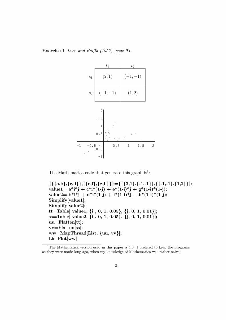
Exercise 1 Luce and Raiffa (1957), page 93.

t1 t2

s1 (2, 1) (−1,−1)

s2 (−1,−1) (1, 2)

-1 -0.5 0.5 1 1.5 2

-1-0.5

0.51

1.52

The Mathematica code that generate this graph is1:

{{{a,b},{c,d}},{{e,f},{g,h}}}={{{2,1},{-1,-1}},{{-1,-1},{1,2}}};value1= a*i*j + c*i*(1-j) + e*(1-i)*j + g*(1-i)*(1-j);value2= b*i*j + d*i*(1-j) + f*(1-i)*j + h*(1-i)*(1-j);Simplify[value1];Simplify[value2];tt=Table[ value1, {i , 0, 1, 0.05}, {j, 0, 1, 0.01}];ss=Table[ value2, {i , 0, 1, 0.05}, {j, 0, 1, 0.01}];uu=Flatten[tt];vv=Flatten[ss];ww=MapThread[List, {uu, vv}];ListPlot[ww]

1The Mathematica version used in this paper is 4.0. I prefered to keep the programsas they were made long ago, when my knowledge of Mathematica was rather naive.

2

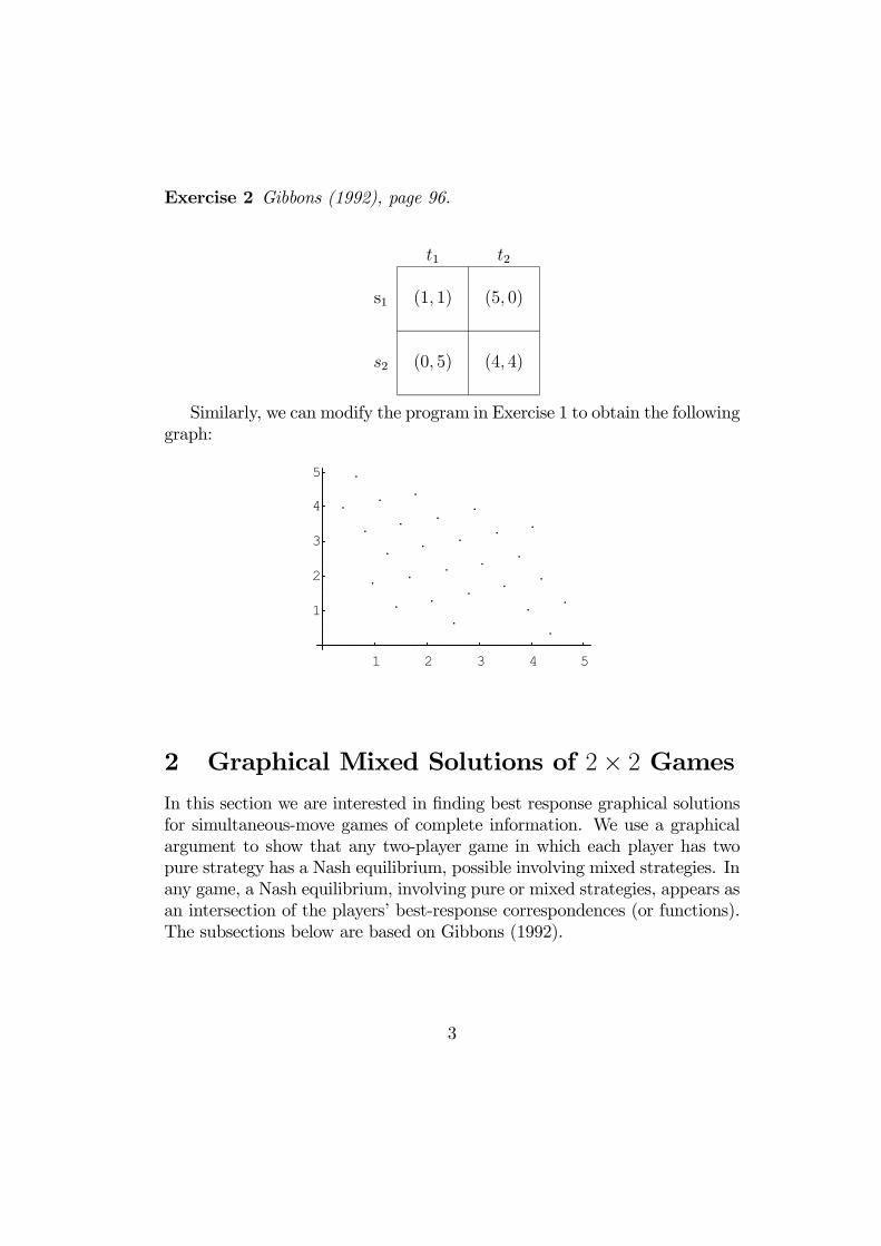
Exercise 2 Gibbons (1992), page 96.

t1 t2

s1 (1, 1) (5, 0)

s2 (0, 5) (4, 4)

Similarly, we can modify the program in Exercise 1 to obtain the followinggraph:

1 2 3 4 5

1

2

3

4

5

2 Graphical Mixed Solutions of 2× 2 GamesIn this section we are interested in finding best response graphical solutionsfor simultaneous-move games of complete information. We use a graphicalargument to show that any two-player game in which each player has twopure strategy has a Nash equilibrium, possible involving mixed strategies. Inany game, a Nash equilibrium, involving pure or mixed strategies, appears asan intersection of the players’ best-response correspondences (or functions).The subsections below are based on Gibbons (1992).

3

2.1 Best Response Functions

The simplest case we can find solving a 2×2 game occurs when there existsdominance between strategies. If a > e and c > g, s1 strictly dominates s2.Accordingly s3 strictly dominates s4 when b > d and f > h. Thus, player1 will play strategy s1 with probability 1, and player 2 will play strategy s3with probability 1. This is shown in Exercise 3.

y 1− ys3 s4

x s1 (a, b) (c, d)

1− x s2 (e, f) (g, h)

Exercise 3

s3 s4

s1 (3, 4) (6, 2)

s2 (2, 5) (5, 3)

The thick line corresponds to player 1 best reponse function, and thedashed line to the best response function of player 2.

4

0.2 0.4 0.6 0.8 1

0.2

0.4

0.6

0.8

1

Exercise 4

s3 s4

s1 (2, 4) (5, 2)

s2 (3, 5) (6, 3)

0.2 0.4 0.6 0.8 1

0.2

0.4

0.6

0.8

1

In order to program a game in Mathematica it is necessary to define thegame in matrix form:

5

game1={{{2,4},{5,2}},{{3,5},{6,3}}}

Then we can apply the Mathematica code for any case involving domi-nance:

{{{a,b},{c,d}},{{e,f},{g,h}}}=game1;If[(a>e) && (c>g) && (b>d), (i=1) && (j=1)];If[(a>e) && (c>g) && (b<d), (i=1) && (j=0)];If[(a<e) && (c<g) && (f>h), (i=0) && (j=1)];If[(a<e) && (c<g) && (b<d), (i=0) && (j=0)];If[(b>d) && (f>h) && (a>e), (i=1) && (j=1)];If[(b>d) && (f>h) && (a<e), (i=0) && (j=1)];If[(b<d) && (f<h) && (c>g), (i=1) && (j=0)];If[(b<d) && (f<h) && (c<g), (i=0) && (j=0)];xx=Table[{i,p2},{p2,0,1,0.01}];yy=Table[{p2,j},{p2,0,1,0.01}];SetOptions[ListPlot, DisplayFunction->Identity];x11=ListPlot[xx,PlotJoined->True, PlotStyle->Thickness[0.01]];y12=ListPlot[yy,PlotJoined->True, PlotStyle->{Thickness[0.0095],Dashing[{0.02}]}];SetOptions[ListPlot, DisplayFunction->$DisplayFunction];If[(i!=2) && (j!=2),Show[x11,y12, DisplayFunction->$DisplayFunction]];

2.2 Best Response Correspondences

If there exists a value of x in which the best response graphs has more thanone value, we will not have functions but correspondences.

Exercise 5 Binmore (1992), page 280.

s3 s4

s1 (1,−1) (4,−4)

s2 (3,−3) (2,−2)

6

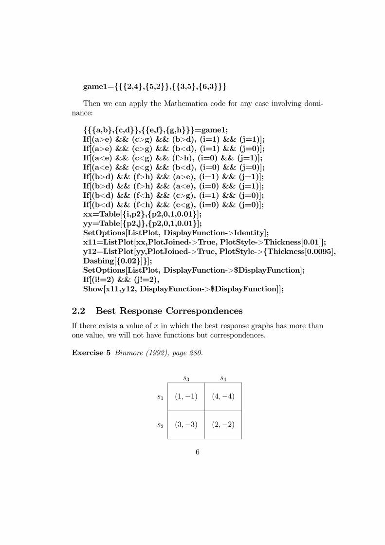
The correspondence for player 1 is

C1 (y) =

{1} if 0 ≤ y ≤ 12

[0, 1] if y = 12{0} if 1

2< y < 1

which in graphical terms becomes

0.2 0.4 0.6 0.8 1

0.2

0.4

0.6

0.8

1

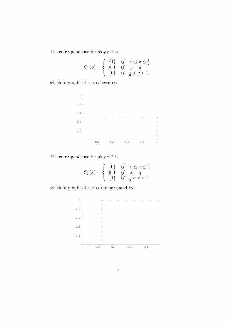
The correspondence for player 2 is

C2 (x) =

{0} if 0 ≤ x ≤ 14

[0, 1] if x = 14{1} if 1

4< x < 1

which in graphical terms is represented by

0.2 0.4 0.6 0.8

0.2

0.4

0.6

0.8

1

7

Thus, the equilibrium in this game appears as an intersection of the play-ers’ best-response:

0.2 0.4 0.6 0.8 1

0.2

0.4

0.6

0.8

1

Exercise 6

s3 s4

s1 (2, 1) (0, 0)

s2 (0, 0) (1, 2)

The graphical solution is

0.2 0.4 0.6 0.8 1

0.2

0.4

0.6

0.8

1

where the square and triangle symbol correspond to player 1 and 2, re-spectively.

8

2.3 Best Response Correspondences with a Contin-uum of Mixed Equilibrium

If we modify the game in Exercise 6 we can illustrate the existence of acontinuum of mixed equilibrium, where one player chooses a mixed strategyand the other player chooses a pure strategy.

Exercise 7

s3 s4

s1 (2, 1) (0, 0)

s2 (2, 0) (1, 2)

The best response for player 1 is now:

0.2 0.4 0.6 0.8 1

0.2

0.4

0.6

0.8

1

The equilibrium for this game involves a convex combination. Any time oneplayer plays the same strategy in two equilibria, then any convex combinationof these strategies is also an equilbrium:

9

0.2 0.4 0.6 0.8 1

0.2

0.4

0.6

0.8

1

To generate the figures in subsections 2.2 aand 2.3 we need to load thepackage MultipleListPlot as follows:

<< Graphics‘MultipleListPlot‘

To draw the graphs and solving the game, we set values in the ”If” linedefined by the payoffs structure. The “If” statement in the first line followsthe algorithm given in Gibbons (1992).

{{{a, b}, {c, d}}, {{e, f}, {g, h}}} = game1;If[(a >= e) && (c <= g) && (b >= d) && (f <= h),V[i_, {p1_, p2_}] := {p1, 1 - p1}.Transpose[game1, {2, 3,

1}][[i]].{p2,1 - p2};aa = V[1, {p1, p2}];bb = V[2, {p1, p2}];cc = Flatten[Solve[D[aa, p1] == 0, p2]];dd = Flatten[Solve[D[bb, p2] == 0, p1]];mixed2 = p2 /. cc;mixed1 = p1 /. dd;ee = p2/2 /. cc;ff = p1/2 /. dd;p2 = ee;p1 = ff;Clear[p1];gg = aa /. p2 -> p2;p1 = ff;

10

Clear[p2];hh = bb /. p1 -> p1;Clear[p1];Clear[p2];ii = D[gg, p1];jj = D[hh, p2];

Testing the slope of functions “ii” and “jj” we can build up the values forthe functions or correspondences that we need to draw.

If[ii < 0, pp1 = 0, pp1 = 1];If[ii < 0, ppp1 = 1, ppp1 = 0];If[jj < 0, pp2 = 0, pp2 = 1];If[jj < 0, ppp2 = 1, ppp2 = 0];oo = Table[{pp1, p2}, {p2, 0, mixed2, 0.1}];pp = Table[{ppp1, p2}, {p2, mixed2, 1, 0.1}];qq = Table[{p1, pp2}, {p1, 0, mixed1, 0.1}];rr = Table[{p1, ppp2}, {p1, mixed1, 1, 0.1}];ss = Table[{mixed1, p2}, {p2, 0, 1, 0.1}];tt = Table[{p1, mixed2}, {p1, 0, 1, 0.1}];

Once we have the “values” we draw using the following code:

zz = MultipleListPlot[oo, pp, tt,SymbolShape -> {PlotSymbol[Box, 2, Filled -> False]}];ww = MultipleListPlot[qq, rr, ss,SymbolShape -> {PlotSymbol[Triangle, 3, Filled -> False]}];Show[zz, ww];Show[GraphicsArray[{zz, ww, yy}]]]

3 Finding Nash equilibrium: The Lyapunovapproach

The problem of finding a Nash equilibrium can be formulated as a problemof finding the minimum of a real valued function. In this approach, everyisolated Nash equilbrium has a basin of attraction. Thus, if one starts closeenough to an isolated Nash equilbrium, then one can guarantee to find itwith any level of accuracy desired (McKelvey and McLennan (1996).

11

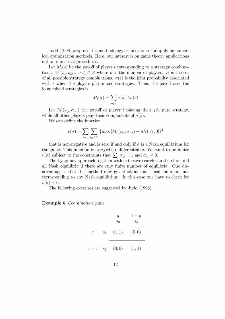
Judd (1998) proposes this methodology as an exercise for applying numer-ical optimization methods. Here, our interest is on game theory applicationsnot on numerical procedures.Let Mi(s) be the payoff of player i corresponding to a strategy combina-

tion s ≡ (s1, s2, ..., sn) ∈ S where n is the number of players. S is the setof all possible strategy combinations. σ(s) is the joint probability associatedwith s when the players play mixed strategies. Then, the payoff over thejoint mixed strategies is

Mi(σ) =Xs∈S

σ(s) Mi(s)

Let Mi(sij, σ−i) the payoff of player i playing their jth pure strategy,while all other players play their components of σ(s).We can define the function

v(σ) =nXi=1

Xsij∈Si

{max [Mi (sij, σ−i)−Mi (σ) , 0]}2

that is non-negative and is zero if and only if σ is a Nash equilibrium forthe game. This function is everywhere differentiable. We want to minimizev(σ) subject to the constraints that

Pj σij = 1 and σij ≥ 0.

The Lyapunov approach together with extensive search can therefore findall Nash equilibria if there are only finite number of equilibria. One dis-advantage is that this method may get stuck at some local minimum notcorresponding to any Nash equilibrium. In this case one have to check forv(σ) = 0.The following exercises are suggested by Judd (1998).

Example 8 Coordination game.

y 1− ys3 s4

x s1 (1, 1) (0, 0)

1− x s2 (0, 0) (1, 1)

12

In this game player 1 play her first strategy with probability x and player2 her first strategy with probability y. First we separate the payoff “matrix”

for player 1 and 2, i.e.,µ1 00 1

¶and find Mi(σ). The input code is:

payoffs={{1,0},{0,1}};misigma={x,1-x}.payoffs.{y,1-y};

The terms Mi (sij, σ−i) for player 1 are:

mplayer11={1,0}.payoffs.{y,1-y};mplayer12={0,1}.payoffs.{y,1-y};

Thus, the first two terms for v(σ) that corresponds to player 1 are:

player11=mplayer11-misigma;player12=mplayer12-misigma;

Similarly, the corresponding terms for player 2 are:

mplayer21={x,1-x}.payoffs.{1,0};mplayer22={x,1-x}.payoffs.{0,1};player21=mplayer21-misigma;player22=mplayer22-misigma;

The function to minimize v(σ) is then:

vsigma=Max[0,player11]^2+Max[0,player12]^2+Max[0,player21]^2+Max[0,player22]^2

Mathematica does not posses a built-in command for an optimizationproblem with constraint, so that, we should impose the constraints as penaltyfunctions, as below:

g1=Max[0, x-1]^2;g2=Max[0,-x]^2;g3=Max[0,y-1]^2;g4=Max[0,-y]^2;

The problem is solved with the FindMinimum procedure which need twostarting points for each variable.

13

FindMinimum[vsigma+1000g1+1000g2+1000g3+1000g4, {x, 0.25,0.2},{y,0.5,0.3}]

The outcomes are x = 0.5 and y = 0.5 and the function value is 1.97215×10−31 ≈ 0.To find a solution may sometimes require judicious choice of a starting

point. We can try with:


The results in this case are x = 1 and y = 1 and the function value is1.821141× 10−17 ≈ 0.Using other starting points give rise to:


The results are x = 4.43378× 10−8 ≈ 0 and y = 3.85761× 10−11 ≈ 0 andthe function value is 1.96584× 10−15 ≈ 0.

An example of a minimum that it is not a Nash equilibrium, can beobtained by:


The outcomes in this case are x = 0.25 and y = 0.25 and the functionvalue is 0.03125 6= 0.Thus, the three equilibria for this game are: {1,0,1,0}; {0.5,0.5,0.5,0.5};{0,1,0,1}.

Exercise 9

x q (1− p− q)t1 t2 t3

x s1 (1, 1) (5, 5) (3, 0)y s2 (1, 7) (6, 4) (1, 1)

(1− x− y) s3 (3, 0) (2, 1) (2, 2)

14

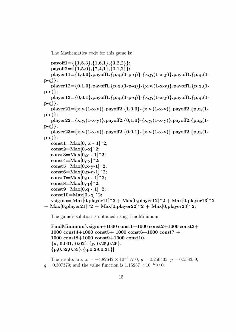
The Mathematica code for this game is:

payoff1={{1,5,3},{1,6,1},{3,2,2}};payoff2={{1,5,0},{7,4,1},{0,1,2}};player11={1,0,0}.payoff1.{p,q,(1-p-q)}-{x,y,(1-x-y)}.payoff1.{p,q,(1-

p-q)};player12={0,1,0}.payoff1.{p,q,(1-p-q)}-{x,y,(1-x-y)}.payoff1.{p,q,(1-

p-q)};player13={0,0,1}.payoff1.{p,q,(1-p-q)}-{x,y,(1-x-y)}.payoff1.{p,q,(1-

p-q)};player21={x,y,(1-x-y)}.payoff2.{1,0,0}-{x,y,(1-x-y)}.payoff2.{p,q,(1-



p-q)};const1=Max[0, x - 1]^2;const2=Max[0,-x]^2;const3=Max[0,y - 1]^2;const4=Max[0,-y]^2;const5=Max[0,x-y-1]^2;const6=Max[0,p-q-1]^2;const7=Max[0,p - 1]^2;const8=Max[0,-p]^2;const9=Max[0,q - 1]^2;const10=Max[0,-q]^2;vsigma=Max[0,player11]^2 +Max[0,player12]^2 +Max[0,player13]^2

+ Max[0,player21]^2 + Max[0,player22]^2 + Max[0,player23]^2;

The game’s solution is obtained using FindMinimum:

FindMinimum[vsigma+1000 const1+1000 const2+1000 const3+1000 const4+1000 const5+ 1000 const6+1000 const7 +1000 const8+1000 const9+1000 const10,{x, 0.001, 0.02},{y, 0.25,0.26},{p,0.52,0.55},{q,0.29,0.31}]

The results are: x = −4.82642× 10−6 ≈ 0, y = 0.250405, p = 0.538359,q = 0.307379; and the value function is 1.15987× 10−6 ≈ 0.

15

A second solution is obtained with:

FindMinimum[vsigma+1000 const1+1000 const2+1000 const3+1000 const4+1000 const5+ 1000 const6+1000 const7 +1000 const8+1000 const9+1000 const10,{x, 0.3, 0.03},{y, 0.3,0.2},{p,0.3,0.2},{q,0.3,0.75}]

The outcomes are: x = −4.98961×10−9 ≈ 0, y = 0.250402, p = 0.602625,q = 0.320525; and the value function is 2.12732× 10−11 ≈ 0.

Therefore, the solutions of this game are:{{0, 0.25, 0.75},{0.538359,0.307379,0.154262} and {{0, 0.25, 0.75}, {0.602665, 0.320525, 0.07}}

Exercise 10 Fudenberg and Tirole (1991), page 55.

y 1− yL R

x U 0, 1, 3 0, 0, 01− x D 1, 1, 1 1, 0, 0

Ap

L RU 2, 2, 2 0, 0, 0D 2, 2, 0 2, 2, 2

Bq

L RU 0, 1, 0 0, 0, 0D 1, 1, 0 1, 0, 3

C1− p− q

First, we work out Mi (sij, σ−i) for player 1. Thus, the code is:

m1=Simplify[{{x,1-x}.{{0,0},{1,1}}.{y,1-y}, {x,1-x}.{{2,0},{2,2}}.{y,1-y},{x,1-x}.{{0,0},{1,1}}.{y,1-y}}.{p,q,1-p-q}];

Similarly, for player 2 and 3:

m2=Simplify[{{x,1-x}.{{1,0},{1,0}}.{y,1-y}, {x,1-x}.{{2,0},{2,2}}.{y,1-y},{x,1-x}.{{1,0},{1,0}}.{y,1-y}}.{p,q,1-p-q}];m3=Simplify[{{x,1-x}.{{3,0},{1,0}}.{y,1-y}, {x,1-x}.{{2,0},{0,2}}.{y,1-

y},{x,1-x}.{{0,0},{0,3}}.{y,1-y}}.{p,q,1-p-q}];

16

The term M1 (sij, σ−i) is obtained replacing (x, 1− x) by (1, 0) in m1:

m11= m1 /. x->1;

Accordingly, all other terms are obtained in the same manner:

m12= m1 /. x->0;m21= m2 /. y->1;m22= m2 /. y->0;m31= m3 /. {p->1, q->0};m32= m3 /. {p->0, q->1};m33= m3 /. {p->0, q->0};

Thus, v(σ) and the constraints are equal to:

vsigma= Max[m11-m1,0]^2 + Max[m12-m1,0]^2 + Max[m21-m2,0]^2 +

Max[m22-m2,0]^2+ Max[m31-m3,0]^2 + Max[m32-m3,0]^2 +Max[m33-m3,0]^2;const1=Max[0, x - 1]^2;const2=Max[0,-x]^2;const3=Max[0,y - 1]^2;const4=Max[0,-y]^2;const5=Max[0,p+q-1]^2;const6=Max[0,p - 1]^2;const7=Max[0,-p]^2;const8=Max[0,q - 1]^2;const9=Max[0,-q]^2;

Finally the minimization problem that we have to solve is:

FindMinimum[vsigma+1000 const1+1000 const2+1000 const3+1000 const4+1000 const5+ 1000 const6+1000 const7 +1000 const8+1000 const9,{x, 0.2, 0.6},{y, 0.2,0.6},{p,0.2,0.6},{q,0.2,0.6}]

which give us the following solution: x = 0.000172152 ≈ 0, y = 0.999848 ≈1, p = 1, q = 0.000013552 ≈ 0; and the value function is 2.41631× 10−7 ≈ 0.The unique equilibrium for this game is: {{0,1},{1,0},{1,0,0}}.

17

References

[1] Binmore, K. (1992). Fun and Games. D.C. Heath and Company.

[2] Fudenberg D. and J. Tirole (1991). Game Theory. MIT Press.

[3] Gibbons, R. (1992). A Primer in Game Theory. Harvester Wheatsheaf.

[4] Judd, K.L. (1998). Numerical Methods in Economics. MIT Press.

[5] Luce, R.D. and H.Raiffa (1957). Games and Decisions. Dover Publica-tions.

[6] McKelvey, D and A. McLenan. (1996). Computation of Equilibria in Fi-nite Games. in H.M Amman .D. Kendrick y J. Rust (eds) Handbook ofComputational Economics, Vol I.

18

game theory exercises 3

Documents