game of life cellular automata || towards a quantum game of life
TRANSCRIPT
Chapter 23Towards a Quantum Game of Life
Adrian P. Flitney and Derek Abbott
Cellular automata provide a means of obtaining complex behaviour from a sim-ple array of cells and a deterministic transition function. They supply a method ofcomputation that dispenses with the need for manipulation of individual cells andthey are computationally universal. Classical cellular automata have proved of greatinterest to computer scientists but the construction of quantum cellular automatapose particular difficulties. We present a version of John Conway’s famous two-dimensional classical cellular automata Life that has some quantum-like features,including interference effects. Some basic structures in the new automata are givenand comparisons are made with Conway’s game.
Landauer based his research on a simple rule: information is physical. That is, informationis registered by physical systems such as strands of DNA, neurons and transistors; in turnthe ways in which systems such as cells, brains and computers can process information isgoverned by the laws of physics. Landauer’s work showed that the apparently simple andunproblematic statement of the physical nature of information had profound consequences.
Seth Lloyd on Rolf Laundauer [21]
23.1 Introductory Concepts of Quantum Mechanics
A good introduction to all aspects of quantum computation is provided by a numberof recent books. The bible remains the excellent work by Nielsen and Chuang [26].In order for the non-specialist to follow this chapter we summarize some conceptsfrom elementary quantum mechanics below.
In the so-called Dirac notation a quantum state labeled by ψ is the ket |ψ〉.The state |ψ〉 is a member of a complex vector space known as a Hilbert space.If {|φi〉, i = 1, . . . ,N} is an orthonormal basis for an N -dimensional Hilbert space,then |ψ〉 may written as the decomposition
|ψ〉 =N∑
i=1
ci |φi〉, (23.1)
where the ci are complex numbers.
A. Adamatzky (ed.), Game of Life Cellular Automata,DOI 10.1007/978-1-84996-217-9_23, © Springer-Verlag London Limited 2010
465
466 A.P. Flitney and D. Abbott
In classical computation, the bit is the fundamental unit of information, takingthe values 0 or 1. The quantum bit or qubit is its quantum analog. The computationalbasis states of a qubit are |0〉 or |1〉. However, a qubit may also be in a superpositionof states, a convex linear combination,
|ψ〉 = α|0〉 + β|1〉, (23.2)
subject to the normalization condition |α|2 + |β|2 = 1. If we examine a qubit to de-termine if it is |0〉 or |1〉, that is, we take a measurement of |ψ〉 in the computationalbasis, the state |0〉 will be returned with probability |α|2 and |1〉 with probability|β|2. The vector
[α
β
], (23.3)
can be used to represent the quantum state (23.2). A superposition is not simply aclassical ensemble of its component states, which would merely represent our lackof knowledge as to whether |ψ〉 is actually |0〉 or |1〉. Instead, each componentof the superposition is simultaneously present. The state (23.2) is often referred toas a coherent superposition to emphasize the existence of coherence between thecomponents. Coherence can be thought of as a measure of the “quantumness” of astate.
Multiple qubits each inhabit their own two-dimensional Hilbert space and can bewritten, for example, as |0〉 ⊗ |1〉 ≡ |01〉. The Hermitian conjugate of a state |φ〉 isknown as the bra φ, or 〈φ|. For example, the Hermitian conjugate of (23.2) is
〈ψ | = α∗〈0| + β∗〈1|, (23.4)
or
[α∗ β∗], (23.5)
where ∗ refers to complex conjugation. The bra-ket 〈φ|ψ〉 measures the overlapbetween two states. That is, |〈φ|ψ〉|2 is the probability of a measurement1 revealing|φ〉 and |ψ〉 in the same state. The two states are orthogonal if this value is zero.If {|φi〉, i = 1, . . . ,N} is an orthonormal basis of an N -dimensional Hilbert space,then |〈φi |φj 〉|2 = δij , where δij is the usual Kronecker delta.
Two or more qubits may exist in an entangled state such as
|ψ〉 = |0〉A ⊗ |0〉B + |1〉A ⊗ |1〉B√2
≡ |0A0B〉 + |1A1B〉√2
. (23.6)
Such a state is not decomposable to a product state of individual qubits. Much ofthe peculiarity of quantum mechanics resides in such states, including Einstein’sfamous “spooky action at a distance” [9], but since they do not concern us in thepresent work they will not be discussed further. Suffice it to say that the measure-ment correlations in the quantum state (23.6) are stronger than can exist in anyclassical system [4].
1We are not going to be concerned with what constitutes a measurement in quantum mechanics,since there is no clear consensus on this. A common sense definition of a measurement will suffice.
23 Semi-quantum Life 467
Fig. 23.1 A classical NOTgate
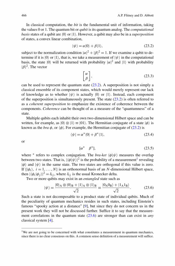
Fig. 23.2 A Hadamard gate
Classical computation is carried out by means of logic gates acting on bits thatare transmitted down wires of some form. The NOT gate, transforming 0 ↔ 1(Fig. 23.1) is the only non-trivial gate on a single bit. The quantum NOT gateswitches |0〉 ↔ |1〉 and acts linearly on a superposition:
α|0〉 + β|1〉 → α|1〉 + β|0〉. (23.7)
The action of the quantum NOT operator X can be represented by the matrix
X ≡[
0 11 0
], (23.8)
where the hat over a symbol indicates that it is an operator. In quantum mechanicsmultiplying a state by an arbitrary phase eiα has no physical effect since the proba-bilities of measurement are proportional to the square of the modulus. However, therelative phase between the components of a superposition is important as we shallsee later. Thus, other important single qubit gates exist in quantum mechanics. Thephase flip operator
Z ≡[
1 00 −1
], (23.9)
has the effect of reversing the relative phase between the |0〉 and |1〉 components ofa superposition, while an arbitrary phase difference is applied by the phase operator
P(α) ≡[
1 00 eiα
]. (23.10)
The Hadamard gate
H ≡ 1√2
[1 11 −1
], (23.11)
changes the computational basis states into a superposition half way between |0〉and |1〉. That is,
H |0〉 = (|0〉 + |1〉)/√2,
H |1〉 = (|0〉 − |1〉)/√2. (23.12)
Note that all operators act linearly on a superposition. Figure 23.2 represents a quan-tum circuit that shows the action of the Hadamard gate. The “wires” represent anymedium through which a qubit can propagate. Any single qubit operation can berepresented by a 2 × 2 unitary matrix, where the overall phase is not physicallyrelevant. An N -qubit operator can be represented by a 2N × 2N unitary matrix.
468 A.P. Flitney and D. Abbott
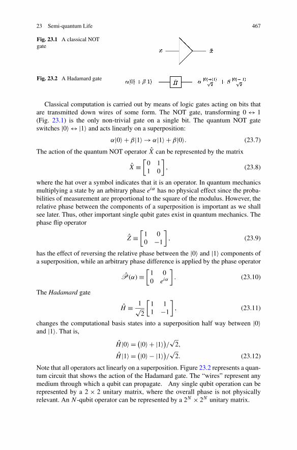
Fig. 23.3 A controlled-NOTgate, where the binaryoperator ⊕ representsaddition modulo two
A particularly useful operator when discussing measurement is the projectionoperator onto the state |φ〉:
P = |φ〉〈φ|. (23.13)
It has the effect of projecting out of a state |ψ〉 only the component parallel with |φ〉.For example, P0 ≡ |0〉〈0| applied to (23.2) results in the state α|0〉. Multi-qubitprojection operators, such as |01〉〈01|, are also possible.
The two-bit gate NAND is known to be universal for classical computation. Thatis, combinations of single-bit gates (NOT gates) and NAND gates can perform anycomputation. In quantum computation all gates are necessarily reversible. Hence,there can be no quantum analogue of the NAND gate, or of the other two-bit gates,AND, OR, and XOR. However, the two-qubit controlled-not, or CNOT, gate to-gether with the set of single-qubit gates forms a universal set for quantum computa-tion [3]. The CNOT gate flips the second qubit if the first, or control qubit, is in the|1〉 state, as shown in Fig. 23.3.
23.2 Background and Motivation for Quantum Life
In this section some of the major results for one-dimensional classical cellular au-tomata are presented and some of the problems of making quantizable versions ofcellular automata are discussed.
23.2.1 Classical Cellular Automata
A cellular automaton (CA) consists of an infinite array of identical cells, the states ofwhich are simultaneously updated in discrete time steps according to a deterministicrule. Formally, they consist of a quadruple (d,Q,N,f ), where d ∈ Z
+ is the dimen-sionality of the array, Q is a finite set of possible states for a cell, N ⊂ Z
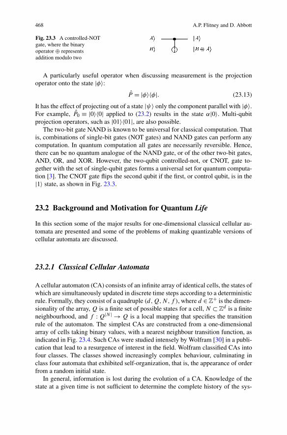
d is a finiteneighbourhood, and f : Q|N | → Q is a local mapping that specifies the transitionrule of the automaton. The simplest CAs are constructed from a one-dimensionalarray of cells taking binary values, with a nearest neighbour transition function, asindicated in Fig. 23.4. Such CAs were studied intensely by Wolfram [30] in a publi-cation that lead to a resurgence of interest in the field. Wolfram classified CAs intofour classes. The classes showed increasingly complex behaviour, culminating inclass four automata that exhibited self-organization, that is, the appearance of orderfrom a random initial state.
In general, information is lost during the evolution of a CA. Knowledge of thestate at a given time is not sufficient to determine the complete history of the sys-
23 Semi-quantum Life 469
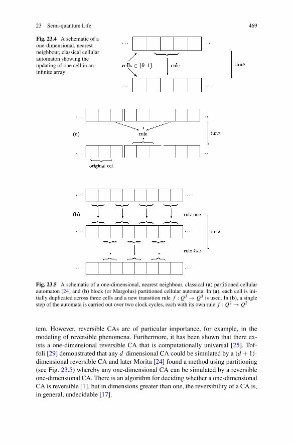
Fig. 23.4 A schematic of aone-dimensional, nearestneighbour, classical cellularautomaton showing theupdating of one cell in aninfinite array
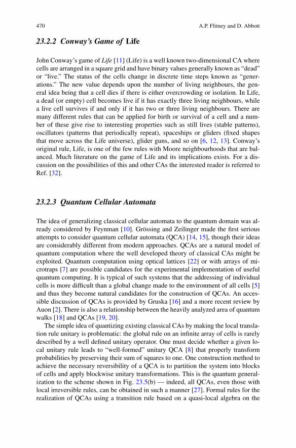
Fig. 23.5 A schematic of a one-dimensional, nearest neighbour, classical (a) partitioned cellularautomaton [24] and (b) block (or Margolus) partitioned cellular automata. In (a), each cell is ini-tially duplicated across three cells and a new transition rule f : Q3 → Q3 is used. In (b), a singlestep of the automata is carried out over two clock cycles, each with its own rule f : Q2 → Q2
tem. However, reversible CAs are of particular importance, for example, in themodeling of reversible phenomena. Furthermore, it has been shown that there ex-ists a one-dimensional reversible CA that is computationally universal [25]. Tof-foli [29] demonstrated that any d-dimensional CA could be simulated by a (d + 1)-dimensional reversible CA and later Morita [24] found a method using partitioning(see Fig. 23.5) whereby any one-dimensional CA can be simulated by a reversibleone-dimensional CA. There is an algorithm for deciding whether a one-dimensionalCA is reversible [1], but in dimensions greater than one, the reversibility of a CA is,in general, undecidable [17].
470 A.P. Flitney and D. Abbott
23.2.2 Conway’s Game of Life
John Conway’s game of Life [11] (Life) is a well known two-dimensional CA wherecells are arranged in a square grid and have binary values generally known as “dead”or “live.” The status of the cells change in discrete time steps known as “gener-ations.” The new value depends upon the number of living neighbours, the gen-eral idea being that a cell dies if there is either overcrowding or isolation. In Life,a dead (or empty) cell becomes live if it has exactly three living neighbours, whilea live cell survives if and only if it has two or three living neighbours. There aremany different rules that can be applied for birth or survival of a cell and a num-ber of these give rise to interesting properties such as still lives (stable patterns),oscillators (patterns that periodically repeat), spaceships or gliders (fixed shapesthat move across the Life universe), glider guns, and so on [6, 12, 13]. Conway’soriginal rule, Life, is one of the few rules with Moore neighbourhoods that are bal-anced. Much literature on the game of Life and its implications exists. For a dis-cussion on the possibilities of this and other CAs the interested reader is referred toRef. [32].
23.2.3 Quantum Cellular Automata
The idea of generalizing classical cellular automata to the quantum domain was al-ready considered by Feynman [10]. Grössing and Zeilinger made the first seriousattempts to consider quantum cellular automata (QCA) [14, 15], though their ideasare considerably different from modern approaches. QCAs are a natural model ofquantum computation where the well developed theory of classical CAs might beexploited. Quantum computation using optical lattices [22] or with arrays of mi-crotraps [7] are possible candidates for the experimental implementation of usefulquantum computing. It is typical of such systems that the addressing of individualcells is more difficult than a global change made to the environment of all cells [5]and thus they become natural candidates for the construction of QCAs. An acces-sible discussion of QCAs is provided by Gruska [16] and a more recent review byAuon [2]. There is also a relationship between the heavily analyzed area of quantumwalks [18] and QCAs [19, 20].
The simple idea of quantizing existing classical CAs by making the local transla-tion rule unitary is problematic: the global rule on an infinite array of cells is rarelydescribed by a well defined unitary operator. One must decide whether a given lo-cal unitary rule leads to “well-formed” unitary QCA [8] that properly transformprobabilities by preserving their sum of squares to one. One construction method toachieve the necessary reversibility of a QCA is to partition the system into blocksof cells and apply blockwise unitary transformations. This is the quantum general-ization to the scheme shown in Fig. 23.5(b) — indeed, all QCAs, even those withlocal irreversible rules, can be obtained in such a manner [27]. Formal rules for therealization of QCAs using a transition rule based on a quasi-local algebra on the
23 Semi-quantum Life 471
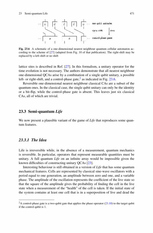
Fig. 23.6 A schematic of a one-dimensional nearest neighbour quantum cellular automaton ac-cording to the scheme of [27] (adapted from Fig. 10 of that publication). The right-shift may bereplaced by a left-shift or no shift
lattice sites is described in Ref. [27]. In this formalism, a unitary operator for thetime evolution is not necessary. The authors demonstrate that all nearest neighbourone-dimensional QCAs arise by a combination of a single qubit unitary, a possibleleft- or right-shift, and a control-phase gate,2 as indicated in Fig. 23.6.
Reversible one-dimensional nearest neighbour classical CAs are a subset of thequantum ones. In the classical case, the single qubit unitary can only be the identityor a bit-flip, while the control-phase gate is absent. This leaves just six classicalCAs, all of which are trivial.
23.3 Semi-quantum Life
We now present a plausible variant of the game of Life that reproduces some quan-tum features.
23.3.1 The Idea
Life is irreversible while, in the absence of a measurement, quantum mechanicsis reversible. In particular, operators that represent measurable quantities must beunitary. A full quantum Life on an infinite array would be impossible given theknown difficulties of constructing unitary QCAs [23].
Interesting behaviour is still obtained in a version of Life that has some quantummechanical features. Cells are represented by classical sine-wave oscillators with aperiod equal to one generation, an amplitude between zero and one, and a variablephase. The amplitude of the oscillation represents the coefficient of the live state sothat the square of the amplitude gives the probability of finding the cell in the livestate when a measurement of the “health” of the cell is taken. If the initial state ofthe system contains at least one cell that is in a superposition of live and dead the
2A control-phase gate is a two-qubit gate that applies the phase operator (23.10) to the target qubitif the control qubit is 1.
472 A.P. Flitney and D. Abbott
neighbouring cells will be influenced according to the coefficients of these states,propagating the superposition to the surrounding region.
If the coefficients of the superpositions are restricted to positive real numbers,qualitatively new phenomena are not expected. By allowing the coefficients to becomplex, that is, by allowing phase differences between the oscillators, qualitativelynew phenomena such as interference effects, may arise. The interference effects seenare those due to an array of classical oscillators with phase shifts and are not fullyquantum mechanical.
23.3.2 A First Model
To represent the state of a cell introduce the following notation:
|ψ〉 = a|live〉 + b|dead〉, (23.14)
subject to the normalization condition
|a|2 + |b|2 = 1. (23.15)
The probability of measuring the cell as live or dead is |a|2 or |b|2, respectively.If the values of a and b are restricted to non-negative real numbers, destructiveinterference does not occur. The model still differs from a classical probabilisticmixture, since here it is the amplitudes that are added and not the probabilities. Inour model |a| is the amplitude of the oscillator. Restricting a to non-negative realnumbers corresponds to the oscillators all being in phase.
The birth, death and survival operators have the following effects:
B|ψ〉 = |live〉,D|ψ〉 = |dead〉, (23.16)
S|ψ〉 = |ψ〉.A cell can be represented by the vector [ a
b ]. The B and D operators are not unitary.Indeed they can be represented in matrix form by
B ∝[
1 10 0
],
(23.17)
D ∝[
0 01 1
],
where the proportionality constant is not relevant for our purposes. After applyingB or D (or some mixture) the new state will require (re-)normalization so that theprobabilities of being dead or live still sum to unity.
A new generation is obtained by determining the number of living neighbourseach cell has and then applying the appropriate operator to that cell. The numberof living neighbours in our model is the amplitude of the superposition of the os-cillators representing the surrounding eight cells. This process is carried out on all
23 Semi-quantum Life 473
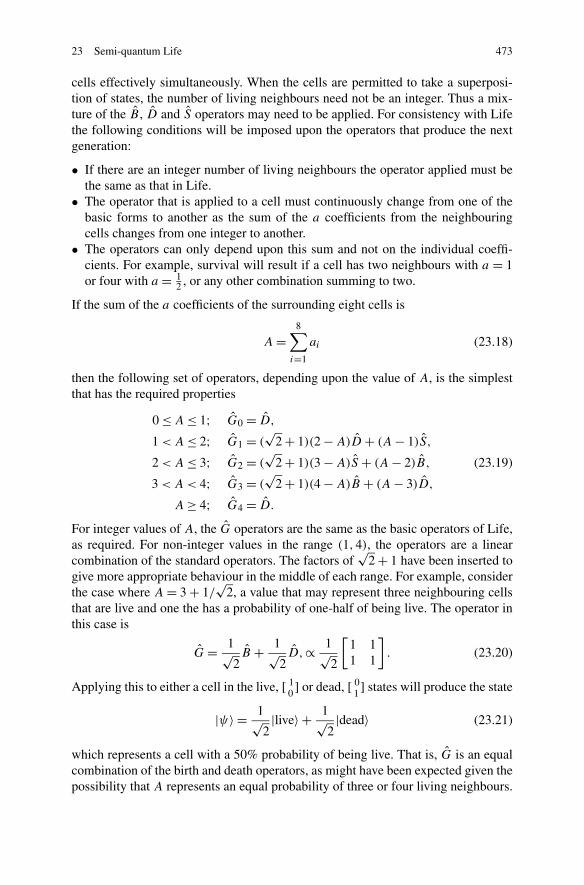
cells effectively simultaneously. When the cells are permitted to take a superposi-tion of states, the number of living neighbours need not be an integer. Thus a mix-ture of the B , D and S operators may need to be applied. For consistency with Lifethe following conditions will be imposed upon the operators that produce the nextgeneration:
• If there are an integer number of living neighbours the operator applied must bethe same as that in Life.
• The operator that is applied to a cell must continuously change from one of thebasic forms to another as the sum of the a coefficients from the neighbouringcells changes from one integer to another.
• The operators can only depend upon this sum and not on the individual coeffi-cients. For example, survival will result if a cell has two neighbours with a = 1or four with a = 1
2 , or any other combination summing to two.
If the sum of the a coefficients of the surrounding eight cells is
A =8∑
i=1
ai (23.18)
then the following set of operators, depending upon the value of A, is the simplestthat has the required properties
0 ≤ A ≤ 1; G0 = D,
1 < A ≤ 2; G1 = (√
2 + 1)(2 − A)D + (A − 1)S,
2 < A ≤ 3; G2 = (√
2 + 1)(3 − A)S + (A − 2)B, (23.19)
3 < A < 4; G3 = (√
2 + 1)(4 − A)B + (A − 3)D,
A ≥ 4; G4 = D.
For integer values of A, the G operators are the same as the basic operators of Life,as required. For non-integer values in the range (1,4), the operators are a linearcombination of the standard operators. The factors of
√2 + 1 have been inserted to
give more appropriate behaviour in the middle of each range. For example, considerthe case where A = 3 + 1/
√2, a value that may represent three neighbouring cells
that are live and one the has a probability of one-half of being live. The operator inthis case is
G = 1√2B + 1√
2D,∝ 1√
2
[1 11 1
]. (23.20)
Applying this to either a cell in the live, [ 10 ] or dead, [ 0
1] states will produce the state
|ψ〉 = 1√2|live〉 + 1√
2|dead〉 (23.21)
which represents a cell with a 50% probability of being live. That is, G is an equalcombination of the birth and death operators, as might have been expected given thepossibility that A represents an equal probability of three or four living neighbours.
474 A.P. Flitney and D. Abbott
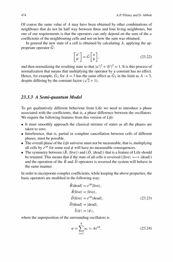
Of course the same value of A may have been obtained by other combinations ofneighbours that do not lie half way between three and four living neighbours, butone of our requirements is that the operators can only depend on the sum of the a
coefficients of the neighbouring cells and not on how the sum was obtained.In general the new state of a cell is obtained by calculating A, applying the ap-
propriate operator G:[a′b′
]= G
[a
b
], (23.22)
and then normalizing the resulting state so that |a′|2 + |b′|2 = 1. It is this process ofnormalization that means that multiplying the operator by a constant has no effect.Hence, for example, G2 for A = 3 has the same effect as G3 in the limit as A → 3,despite differing by the constant factor (
√2 + 1).
23.3.3 A Semi-quantum Model
To get qualitatively different behaviour from Life we need to introduce a phaseassociated with the coefficients, that is, a phase difference between the oscillators.We require the following features from this version of Life:
• It must smoothly approach the classical mixture of states as all the phases aretaken to zero.
• Interference, that is, partial or complete cancellation between cells of differentphases, must be possible.
• The overall phase of the Life universe must not be measurable, that is, multiplyingall cells by eiφ for some real φ will have no measurable consequences.
• The symmetry between (B, |live〉) and (D, |dead〉) that is a feature of Life shouldbe retained. This means that if the state of all cells is reversed (|live〉 ←→ |dead〉)and the operation of the B and D operators is reversed the system will behave inthe same manner.
In order to incorporate complex coefficients, while keeping the above properties, thebasic operators are modified in the following way:
B|dead〉 = eiφ |live〉,B|live〉 = |live〉,D|live〉 = eiφ |dead〉, (23.23)
D|dead〉 = |dead〉,S|ψ〉 = |ψ〉,
where the superposition of the surrounding oscillators is
α =8∑
i=1
ai = Aeiφ, (23.24)
23 Semi-quantum Life 475
A and φ being real positive numbers. That is, the birth and death operators are mod-ified so that the new live or dead state has the phase of the sum of the surroundingcells. The operation of the B and D operators on the state [ a
b ] can be written as
B
[a
b
]=
[a + |b|eiφ
0
],
(23.25)
D
[a
b
]=
[0
|a|eiφ + b
],
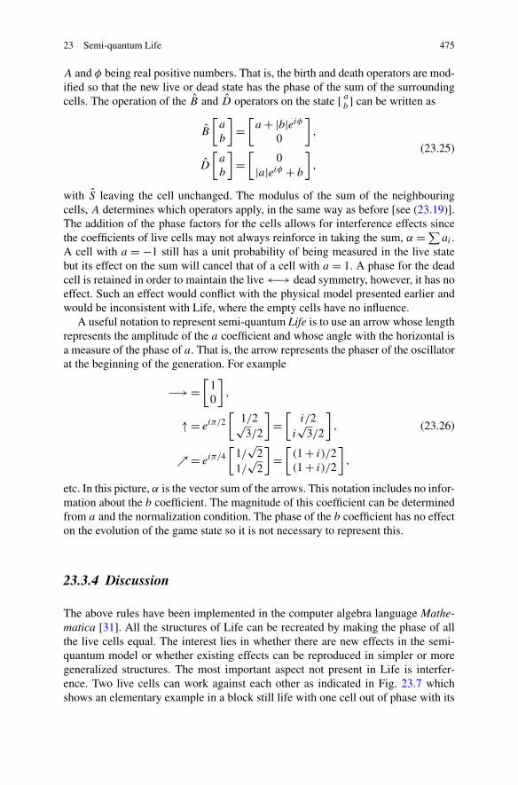
with S leaving the cell unchanged. The modulus of the sum of the neighbouringcells, A determines which operators apply, in the same way as before [see (23.19)].The addition of the phase factors for the cells allows for interference effects sincethe coefficients of live cells may not always reinforce in taking the sum, α = ∑
ai .A cell with a = −1 still has a unit probability of being measured in the live statebut its effect on the sum will cancel that of a cell with a = 1. A phase for the deadcell is retained in order to maintain the live ←→ dead symmetry, however, it has noeffect. Such an effect would conflict with the physical model presented earlier andwould be inconsistent with Life, where the empty cells have no influence.
A useful notation to represent semi-quantum Life is to use an arrow whose lengthrepresents the amplitude of the a coefficient and whose angle with the horizontal isa measure of the phase of a. That is, the arrow represents the phaser of the oscillatorat the beginning of the generation. For example
−→ =[
10
],
↑ = eiπ/2[
1/2√3/2
]=
[i/2
i√
3/2
], (23.26)
↗ = eiπ/4[
1/√
21/
√2
]=
[(1 + i)/2(1 + i)/2
],
etc. In this picture, α is the vector sum of the arrows. This notation includes no infor-mation about the b coefficient. The magnitude of this coefficient can be determinedfrom a and the normalization condition. The phase of the b coefficient has no effecton the evolution of the game state so it is not necessary to represent this.
23.3.4 Discussion
The above rules have been implemented in the computer algebra language Mathe-matica [31]. All the structures of Life can be recreated by making the phase of allthe live cells equal. The interest lies in whether there are new effects in the semi-quantum model or whether existing effects can be reproduced in simpler or moregeneralized structures. The most important aspect not present in Life is interfer-ence. Two live cells can work against each other as indicated in Fig. 23.7 whichshows an elementary example in a block still life with one cell out of phase with its
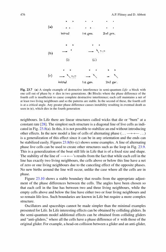
476 A.P. Flitney and D. Abbott
Fig. 23.7 (a) A simple example of destructive interference in semi-quantum Life: a block withone cell out of phase by π dies in two generations. (b) Blocks where the phase difference of thefourth cell is insufficient to cause complete destructive interference; each cell maintains a net ofat least two living neighbours and so the patterns are stable. In the second of these, the fourth cellis at a critical angle. Any greater phase difference causes instability resulting in eventual death asseen in (c), which dies in the fourth generation
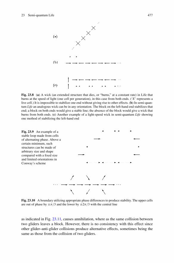
neighbours. In Life there are linear structures called wicks that die or “burn” at aconstant rate [28]. The simplest such structure is a diagonal line of live cells as indi-cated in Fig. 23.8(a). In this, it is not possible to stabilize an end without introducingother effects. In the new model a line of cells of alternating phase (. . . −→←− . . .)is a generalization of this effect since it can be in any orientation and the ends canbe stabilized easily. Figures 23.8(b)–(c) shows some examples. A line of alternatingphase live cells can be used to create other structures such as the loop in Fig. 23.9.This is a generalization of the boat still life in Life that is of a fixed size and shape.The stability of the line of −→←−’s results from the fact that while each cell in theline has exactly two living neighbours, the cells above or below this line have a netof zero or one living neighbours due to the canceling effect of the opposite phases.No new births around the line will occur, unlike the case where all the cells are inphase.
Figure 23.10 shows a stable boundary that results from the appropriate adjust-ment of the phase differences between the cells. The angles have been chosen sothat each cell in the line has between two and three living neighbours, while theempty cells above and below the line have either two or four living neighbours andso remain life-less. Such boundaries are known in Life but require a more complexstructure.
Oscillators and spaceships cannot be made simpler than the minimal examplespresented for Life. In Life interesting effects can be obtained by colliding gliders. Inthe semi-quantum model additional effects can be obtained from colliding glidersand “anti-gliders,” where all the cells have a phase difference of π with those of theoriginal glider. For example, a head-on collision between a glider and an anti-glider,
23 Semi-quantum Life 477
Fig. 23.8 (a) A wick (an extended structure that dies, or “burns,” at a constant rate) in Life thatburns at the speed of light (one cell per generation), in this case from both ends. (‘X’ represents alive cell.) It is impossible to stabilize one end without giving rise to other effects. (b) In semi-quan-tum Life an analogous wick can be in any orientation. The block on the left-hand end stabilizes thatend; a block on both ends would give a stable line; the absence of the block would give a wick thatburns from both ends. (c) Another example of a light-speed wick in semi-quantum Life showingone method of stabilizing the left-hand end
Fig. 23.9 An example of astable loop made from cellsof alternating phase. Above acertain minimum, suchstructures can be made ofarbitrary size and shapecompared with a fixed sizeand limited orientations inConway’s scheme
Fig. 23.10 A boundary utilizing appropriate phase differences to produce stability. The upper cellsare out of phase by ±π/3 and the lower by ±2π/3 with the central line
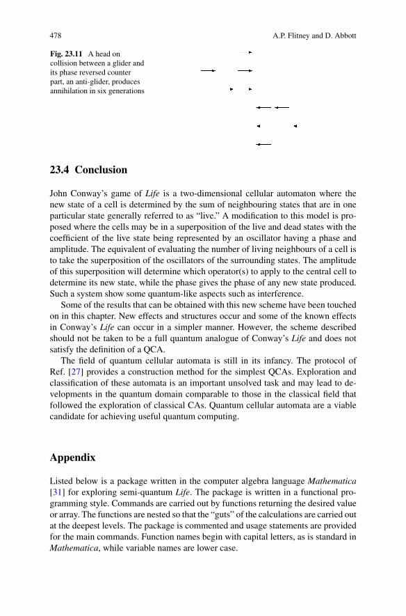
as indicated in Fig. 23.11, causes annihilation, where as the same collision betweentwo gliders leaves a block. However, there is no consistency with this effect sinceother glider–anti-glider collisions produce alternative effects, sometimes being thesame as those from the collision of two gliders.
478 A.P. Flitney and D. Abbott
Fig. 23.11 A head oncollision between a glider andits phase reversed counterpart, an anti-glider, producesannihilation in six generations
23.4 Conclusion
John Conway’s game of Life is a two-dimensional cellular automaton where thenew state of a cell is determined by the sum of neighbouring states that are in oneparticular state generally referred to as “live.” A modification to this model is pro-posed where the cells may be in a superposition of the live and dead states with thecoefficient of the live state being represented by an oscillator having a phase andamplitude. The equivalent of evaluating the number of living neighbours of a cell isto take the superposition of the oscillators of the surrounding states. The amplitudeof this superposition will determine which operator(s) to apply to the central cell todetermine its new state, while the phase gives the phase of any new state produced.Such a system show some quantum-like aspects such as interference.
Some of the results that can be obtained with this new scheme have been touchedon in this chapter. New effects and structures occur and some of the known effectsin Conway’s Life can occur in a simpler manner. However, the scheme describedshould not be taken to be a full quantum analogue of Conway’s Life and does notsatisfy the definition of a QCA.
The field of quantum cellular automata is still in its infancy. The protocol ofRef. [27] provides a construction method for the simplest QCAs. Exploration andclassification of these automata is an important unsolved task and may lead to de-velopments in the quantum domain comparable to those in the classical field thatfollowed the exploration of classical CAs. Quantum cellular automata are a viablecandidate for achieving useful quantum computing.
Appendix
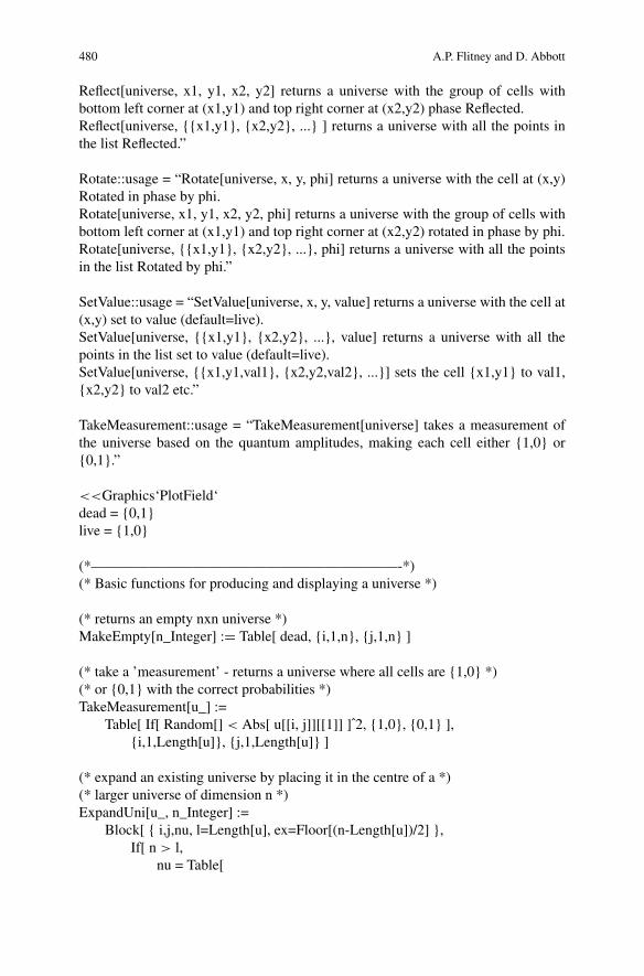
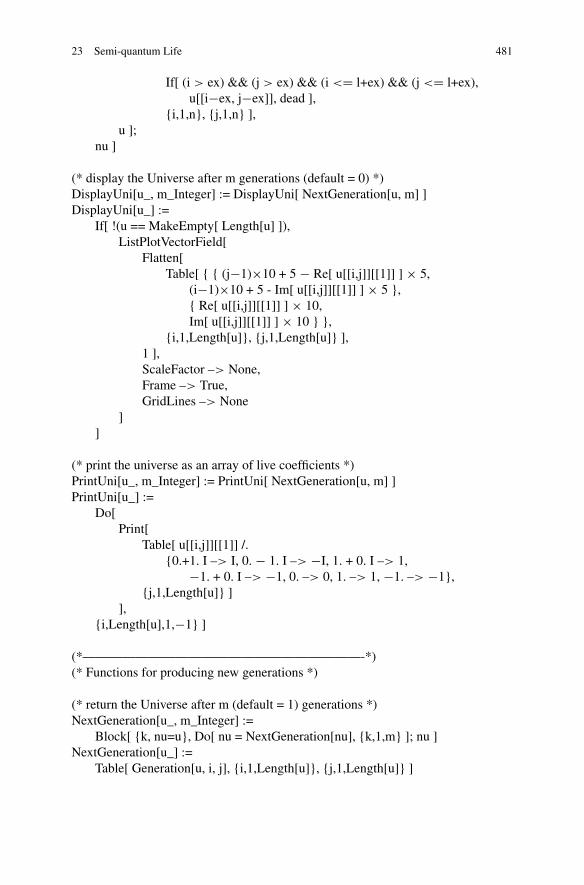
Listed below is a package written in the computer algebra language Mathematica[31] for exploring semi-quantum Life. The package is written in a functional pro-gramming style. Commands are carried out by functions returning the desired valueor array. The functions are nested so that the “guts” of the calculations are carried outat the deepest levels. The package is commented and usage statements are providedfor the main commands. Function names begin with capital letters, as is standard inMathematica, while variable names are lower case.

23 Semi-quantum Life 479
CountNeigh::usage = “CountNeigh[universe, x, y] returns the sum of the live coef-ficients of the cells surrounding (x,y).”
DisplayUni::usage = “DisplayUni[universe] displays a graphic of the universe witharrows representing living cells, the length being the magnitude and the angle withthe horizontal being the phase.DisplayUni[universe, m] displays the universe after m generations.”
ExpandUni::usage = “ExpandUni[universe, n] returns an nxn universe with the olduniverse centred in it. n must be larger than the existing universe dimensions.”
Generation::usage = “Generation[universe, x, y] returns a universe with the newvalue of the cell at (x,y).”
InsertBlinker::usage = “InsertBlinker[universe, x, y] returns a universe with the ad-dition of a blinker (horizontal) starting at (x,y).”
InsertBlock::usage = “InsertBlock[universe, x, y] returns a universe with the addi-tion of a block (2x2 square of live cells) with the lower left corner (x,y).InsertBlock[universe, x1, y1, x2, y2] returns a universe with the addition of a groupof live cells with lower left corner (x1,y1) and upper right corner (x2,y2).”
InsertGlider::usage = “InsertGlider[universe, x, y, dir] returns a universe with theaddition of a glider with the lower left corner of the 3x3 square containing the gliderat (x,y). dir gives the direction of the glider NE, NW, SW, SE.”
InsertLine::usage = “InsertLine[universe, x, y, m] returns universe with the additionof a line of live cells starting at (x,y) of length |m|. The line is horizontal if m ispositive, vertical if m is negative.”
InsertString::usage = “InsertString[universe, x, y, m] returns a universe with theaddition of a line of live cells of alternating phase (a ‘string’) of length |m|. The lineis horizontal if m is positive, vertical if m is negative.”
MakeUni::usage = “MakeUni[n] returns an empty universe of dimension nxn.”
NextGeneration::usage = “NextGeneration[universe] returns the next generation ofthe universe.NextGeneration[universe, m] returns the universe after m generations.”
NormaliseCell::usage = “NormaliseCell[cell] returns the normalised value of thegiven cell. All cells are automatically normalised when producing the next genera-tion by the function Generations.”
Reflect::usage = “Reflect[universe, x, y] returns a universe with the cell at (x,y)phase Reflected. i.e., {1,0} –> {−1,0}.
480 A.P. Flitney and D. Abbott
Reflect[universe, x1, y1, x2, y2] returns a universe with the group of cells withbottom left corner at (x1,y1) and top right corner at (x2,y2) phase Reflected.Reflect[universe, {{x1,y1}, {x2,y2}, ...} ] returns a universe with all the points inthe list Reflected.”
Rotate::usage = “Rotate[universe, x, y, phi] returns a universe with the cell at (x,y)Rotated in phase by phi.Rotate[universe, x1, y1, x2, y2, phi] returns a universe with the group of cells withbottom left corner at (x1,y1) and top right corner at (x2,y2) rotated in phase by phi.Rotate[universe, {{x1,y1}, {x2,y2}, ...}, phi] returns a universe with all the pointsin the list Rotated by phi.”
SetValue::usage = “SetValue[universe, x, y, value] returns a universe with the cell at(x,y) set to value (default=live).SetValue[universe, {{x1,y1}, {x2,y2}, ...}, value] returns a universe with all thepoints in the list set to value (default=live).SetValue[universe, {{x1,y1,val1}, {x2,y2,val2}, ...}] sets the cell {x1,y1} to val1,{x2,y2} to val2 etc.”
TakeMeasurement::usage = “TakeMeasurement[universe] takes a measurement ofthe universe based on the quantum amplitudes, making each cell either {1,0} or{0,1}.”
<<Graphics‘PlotField‘dead = {0,1}live = {1,0}
(*—————————————————————-*)(* Basic functions for producing and displaying a universe *)
(* returns an empty nxn universe *)MakeEmpty[n_Integer] := Table[ dead, {i,1,n}, {j,1,n} ]
(* take a ’measurement’ - returns a universe where all cells are {1,0} *)(* or {0,1} with the correct probabilities *)TakeMeasurement[u_] :=
Table[ If[ Random[] < Abs[ u[[i, j]][[1]] ]ˆ2, {1,0}, {0,1} ],{i,1,Length[u]}, {j,1,Length[u]} ]
(* expand an existing universe by placing it in the centre of a *)(* larger universe of dimension n *)ExpandUni[u_, n_Integer] :=
Block[ { i,j,nu, l=Length[u], ex=Floor[(n-Length[u])/2] },If[ n > l,
nu = Table[
23 Semi-quantum Life 481
If[ (i > ex) && (j > ex) && (i <= l+ex) && (j <= l+ex),u[[i−ex, j−ex]], dead ],
{i,1,n}, {j,1,n} ],u ];
nu ]
(* display the Universe after m generations (default = 0) *)DisplayUni[u_, m_Integer] := DisplayUni[ NextGeneration[u, m] ]DisplayUni[u_] :=
If[ !(u == MakeEmpty[ Length[u] ]),ListPlotVectorField[
Flatten[Table[ { { (j−1)×10 + 5 − Re[ u[[i,j]][[1]] ] × 5,
(i−1)×10 + 5 - Im[ u[[i,j]][[1]] ] × 5 },{ Re[ u[[i,j]][[1]] ] × 10,Im[ u[[i,j]][[1]] ] × 10 } },
{i,1,Length[u]}, {j,1,Length[u]} ],1 ],ScaleFactor –> None,Frame –> True,GridLines –> None
]]
(* print the universe as an array of live coefficients *)PrintUni[u_, m_Integer] := PrintUni[ NextGeneration[u, m] ]PrintUni[u_] :=
Do[Print[
Table[ u[[i,j]][[1]] /.{0.+1. I –> I, 0. − 1. I –> −I, 1. + 0. I –> 1,
−1. + 0. I –> −1, 0. –> 0, 1. –> 1, −1. –> −1},{j,1,Length[u]} ]
],{i,Length[u],1,−1} ]
(*—————————————————————-*)(* Functions for producing new generations *)
(* return the Universe after m (default = 1) generations *)NextGeneration[u_, m_Integer] :=
Block[ {k, nu=u}, Do[ nu = NextGeneration[nu], {k,1,m} ]; nu ]NextGeneration[u_] :=
Table[ Generation[u, i, j], {i,1,Length[u]}, {j,1,Length[u]} ]
482 A.P. Flitney and D. Abbott
(* generate the new value of the cell at position (x,y) *)Generation[u_, x_, y_] :=
Block[ {neigh=0, phi, A, cell=u[[x, y]], newcell={0,0}},neigh = CountNeigh[u, x, y];A = Abs[neigh];If[ !(neigh == 0), phi = Arg[neigh], phi=0 ];Which[
(A <= 1) || (A >= 4), newcell = Death[cell, phi],(A > 1) && (A <= 2), newcell = (Sqrt[2] + 1)(A−1) cell +
(2−A) Death[cell, phi],(A > 2) && (A <= 3), newcell = (Sqrt[2] + 1)(A−2) ×
Birth[cell, phi] + (3−A) cell,(A > 3) && (A < 4), newcell = (Sqrt[2] + 1)(A−3) ×
Death[cell, phi] + (4−A) Birth[cell, phi]];NormaliseCell[newcell]
]
(* count the number of neighbours to cell (x,y) *)CountNeigh[u_, x_, y_] :=
Block[ {temp=0, n=Length[u]},If[ (x > 1) && (y > 1), temp += u[[x−1, y−1]][[1]] ];If[ (x > 1), temp += u[[x−1, y]][[1]] ];If[ (x > 1) && (y < n), temp += u[[x−1, y+1]][[1]] ];If[ (y > 1), temp += u[[x, y−1]][[1]] ];If[ (y < n), temp += u[[x, y+1]][[1]] ];If[ (x < n) && (y > 1), temp += u[[x+1, y−1]][[1]] ];If[ (x < n), temp += u[[x+1, y]][[1]] ];If[ (x < n) && (y < n), temp += u[[x+1, y+1]][[1]] ];
temp ]
(* B, D operators *)Birth[c_, phi_] := {c[[1]] + Exp[I phi] × Abs[ c[[2]] ], 0}Death[c_, phi_] := {0, c[[2]] + Exp[I phi] × Abs[ c[[1]] ]}
(* normalise a cell so |a|ˆ2 + |b|ˆ2 = 1 *)NormaliseCell[c_] :=
Block[ {normfact=Sqrt[ Abs[c[[1]]]ˆ2 + Abs[c[[2]]ˆ2] ], nc = dead},If[ !(normfact == 0),
( nc[[1]] = c[[1]]/normfact;nc[[2]] = c[[2]]/normfact )
];N[nc]
]
23 Semi-quantum Life 483
(*———————————————————————–*)(* Functions for setting cell and manipulating cell values *)
(* set the (x,y) cell in u to value val (default=live) *)SetValue[u_, x_Integer, y_Integer] := SetValue[u, x, y, live]SetValue[u_, x_Integer, y_Integer, val_] :=
Block[ {nu = u}, nu[[x, y]] = val; nu](* set the list of points to the specified value (default=live) *)SetValue[u_, pts_List] := SetValue[u, pts, live]SetValue[u_, pts_List, val_] :=
Block[ {i, nu = u},Do[ nu[[ pts[[i]][[1]], pts[[i]][[2]] ]] = val,{i,1,Length[pts]} ];
nu ](* set a list of points to the specified individual values *)SetValue[u_, pts_List] :=
Block[ {i, nu=u},Do[ nu = SetValue[ nu, pts[[i]][[1]], pts[[i]][[2]], pts[[i]][[3]] ],{i,Length[pts]} ];
nu ]
(* Reflect the phase of the live coefficient of the cell at (x,y) *)Reflect[u_, x_Integer, y_Integer] :=
SetValue[ u, x, y, {−u[[x, y]][[1]], u[[x, y]][[2]]} ]
(* Reflect the phase of a group of cells with bottom left corner (x1,y1) *)(* and top right corner (x2,y2). *)Reflect[u_, x1_Integer, y1_Integer, x2_Integer, y2_Integer] :=
Block[ {i,j, nu=u},Do[ nu = Reflect[ nu, i, j ], {i,x1,x2}, {j,y1,y2} ];
nu ]
(* Reflect the list of points in ‘pts’ *)Reflect[u_, pts_List] :=
Block[ {i, nu=u},Do[ nu = Reflect[ nu, pts[[i]][[1]], pts[[i]][[2]] ],{i,1,Length[pts]} ];
nu ]
(* Rotate the live coefficient of the cell at (x,y) by phi *)Rotate[u_, x_Integer, y_Integer, phi_] := SetValue[ u, x, y,
{u[[x, y]][[1]] * Exp[I phi], u[[x, y]][[2]]} ]
(* Rotates a group of cells with bottom left corner (x1,y1) and top right *)(* corner (x2,y2), by phi *)
484 A.P. Flitney and D. Abbott
Rotate[u_, x1_Integer, y1_Integer, x2_Integer, y2_Integer, phi_] :=Block[ {i,j, nu=u},
Do[ nu = Rotate[nu, i, j, phi], {i,x1,x2}, {j,y1,y2} ];nu ]
(* Rotate the list of points in the list ‘pts’ by phi *)Rotate[u_, pts_List, phi_] :=
Block[ {i, nu=u},Do[ nu = Rotate[ nu, pts[[i]][[1]], pts[[i]][[2]], phi ],{i,1,Length[pts]} ];
nu ]
(*—————————————————————*)(* Some functions for inserting certain structures *)
(* blinker (period two oscillator – horizontal – starting at (x,y) *)InsertBlinker[u_, x_Integer, y_Integer] :=
Block[ {nu=u}, Do[ nu = SetValue[nu, x, y+i, live], {i,0,2} ]; nu ]
(* block still life, lower left corner at (x,y) *)InsertBlock[u_, x_Integer, y_Integer] :=
Block[ {nu=u},Do[ nu = SetValue[nu, i, j, live], {i,x,x+1}, {j,y,y+1} ];
nu ]
(* set a block of cells to a value, (default = live) *)InsertBlock[u_, x1_Integer, y1_Integer, x2_Integer, y2_Integer] :=
InsertBlock[u, x1, y1, x2, y2, live]InsertBlock[u_, x1_Integer, y1_Integer, x2_Integer, y2_Integer, val_] :=
Block[ {nu=u},Do[ nu = SetValue[nu, i, j, live], {i,x1,x2}, {j,y1,y2} ];
nu ]
(* Insert a glider, lower corner of 3x3 square containing glider at (x,y) *)(* dir specifies the direction *)InsertGlider[u_, x_Integer, y_Integer, dir_] :=
Block[ {nu=u},Which[
dir == “se”) || (dir == “SE”),nu = SetValue[nu, x, y+1, live];nu = SetValue[nu, x−1, y+2, live];Do[ nu = SetValue[nu, x−2, y+i, live], {i,0,2} ],
(dir == “sw”) || (dir == “SW”),
23 Semi-quantum Life 485
nu = SetValue[nu, x−2, y+1, live];nu = SetValue[nu, x−1, y+2, live];Do[ nu = SetValue[nu, x−i, y, live], {i,0,2} ],
(dir == “nw”) || (dir == “NW”),nu = SetValue[nu, x−1, y, live];nu = SetValue[nu, x−2, y+1, live];Do[ nu = SetValue[nu, x, y+i, live], {i,0,2} ],
(dir == “ne”) || (dir == “NE”),nu = SetValue[nu, x−1, y, live];nu = SetValue[nu, x, y+1, live];Do[ nu = SetValue[nu, x−i, y+2, live], {i,0,2} ]
];nu ]
(* insert a line of live cells starting at (x,y) of length |m| *)(* horizontal if m > 0, vertical if m < 0 *)InsertLine[u_, x_Integer, y_Integer, m_Integer] :=
Block[ {nu=u, i},If[m > 0,
Do[nu = SetValue[nu, x, y + i, live], {i, 0, m−1}],Do[nu = SetValue[nu, x + i, y, live], {i, 0, −m−1}]
];nu ]
(* horizontal‘string’ starting at (x,y) of length m, if m > 0 *)(* or a vertical ‘string’ starting at (x,y) of length −m, if m < 0 *)(* string starts with {1,0} *)InsertString[u_, x_Integer, y_Integer, m_Integer] :=
Block[ {nu=u, i},If[m > 0,
Do[nu = SetValue[nu, x, y + i, {(-1)ˆi, 0}], {i, 0, m−1}],Do[nu = SetValue[nu, x + i, y, {(-1)ˆi, 0}], {i, 0, −m−1}]
];nu ]
References
1. Amoroso, S., Patt, Y.N.: Decision procedures for surjectivity and injectivity of parallel mapsfor tessellation structures. J. Comput. Syst. Sci. 6, 448–464 (1972)
2. Auon, B., Tarifi, M.: Introduction to quantum cellular automata. Eprint: arXiv:quant-ph/0401123 (2004)
3. Barenco, A., Bennett, C.H., Cleve, R., DiVincenzo, D.P., Margolus, N., Shor, P., Sleator, J.,Smolin J., Weinfurter, H.: Elementary gates for quantum computation. Phys. Rev. A 52, 3457–3467 (1995)
4. Bell, J.S.: On the Einstein–Podolsky–Rosen paradox. Physics 1, 195–200 (1964)
486 A.P. Flitney and D. Abbott
5. Benjamin, S.C.: Schemes for parallel quantum computation without local control of qubits.Phys. Rev. A 61, 020301 (2000)
6. Berlekamp, E.R., Conway, J.H., Guy, R.K.: Winning Ways for Your Mathematical Plays,vol. 2. Academic Press, London (1982)
7. Dumke, R., Volk, M., Muether, T., Buchkremer, F.B.J., Birkl, G., Ertmer, W.: Microoptical re-alization of arrays of selectively addressable dipole traps: a scalable configuration for quantumcomputation with atomic qubits. Phys. Rev. Lett. 89, 097903 (2002)
8. Dürr, C., Santha, M.: A decision procedure for well-formed unitary linear quantum cellularautomata. SIAM J. Comput. 31, 1076–1089 (2002)
9. Einstein, A., Podolsky, B., Rosen, N.: Can quantum-mechanical description of physical realitybe considered complete? Phys. Rev. 47, 777–780 (1935)
10. Feynman, R.P.: Simulating physics with computers. Int. J. Theor. Phys. 21, 467–488 (1982)11. Gardner, M.: Mathematical games: The fantastic combinations of John Conway’s new solitaire
game of “Life”. Sci. Am. 223(10), 120 (1970)12. Gardner, M.: Mathematical games: On cellular automata, self-reproduction, the Garden of
Eden and the game of “Life”. Sci. Am. 224(2), 116 (1971)13. Gardner, M.: Wheels, Life and Other Mathematical Amusements. Freeman, New York (1983)14. Grössing, G., Zeilinger, A.: Quantum cellular automata. Complex Syst. 2, 197–208 (1988)15. Grössing, G., Zeilinger, A.: Structures in quantum cellular automata. Physica B 151, 366–370
(1988)16. Gruska, J.: Quantum Computing. McGraw Hill, Maidenhead (1999)17. Kari, J.: Reversibility of two-dimensional cellular automata is undecidable. Physica D 45,
379–385 (1990)18. Kempe, J.: Quantum random walks: an introductory overview. Contemp. Phys. 44, 307–327
(2003)19. Konno, N.: Quantum Walks and Quantum Cellular Automata. Lecture Notes in Computer
Science. Springer, Berlin/Heidelberg (2008)20. Konno, N., Mistuda, K., Soshi, T., Yoo, H.J.: Quantum walks and reversible cellular automata.
Phys. Lett. A 330, 408–417 (2004)21. Lloyd, S.: Obituary: Rolf Laundauer. Nature 400, 720 (1999)22. Mandel, D., Greiner, M., Widera, A., Rom, T., Hänsch, T.W., Bloch, I.: Coherent transport of
neutral atoms in spin-dependent optical lattice potentials. Phys. Rev. Lett. 91, 010407 (2003)23. Meyer, D.A.: From quantum cellular automata to quantum lattice gases. J. Stat. Phys. 85,
551–574 (1996)24. Morita, K.: Reversible simulation of one-dimensional irreversible cellular automata. Theor.
Comput. Sci. 148, 157–163 (1995)25. Morita, K., Harao, M.: Computation universality of one-dimensional reversible (injective) cel-
lular automata. Trans. IEICE 72, 758–762 (1989)26. Nielsen, M.A., Chuang, I.: Quantum Computation and Quantum Information. Cambridge Uni-
versity Press, Cambridge (2000)27. Schumacher, B., Werner, R.F.: Reversible quantum cellular automata. Eprint: arXiv:quant-ph/
0405174 (2004)28. Silver, S.A.: http://www.bitstorm.org/gameoflife/lexicon29. Toffoli, T.: Cellular automata mechanics. PhD thesis, The University of Michigan (1977)30. Wolfram, S.: Statistical mechanics of cellular automata. Rev. Mod. Phys. 55, 601–644 (1983)31. Wolfram, S.: Mathematica: A System for Doing Mathematics by Computer. Addison–Wesley,
Redwood City (1988)32. Wolfram, S.: A New Kind of Science. Wolfram Media, Champaign (2002)