Stylized Facts Generated Through Cellular Automata Models.

Case of Study: The Game of Life

A.R. Hernandez-Montoya, H.F. Coronel-Brizio, and G.A. Stevens-RamırezDepartamento de Inteligencia Artificial, Facultad de Fısica e Inteligencia Artificial,Universidad Veracruzana. Sebastian Camacho 5, Xalapa Veracruz 91000, Mexico.

M. Rodrıguez-AchachDepartamento de Fısica. Facultad de Fısica e Inteligencia Artificial,

Universidad Veracruzana, Lomas del Estadio S/N, Xalapa, Veracruz, Mexico.

M. PolitiSSRI & Department of Economics and Business,

International Christian University,3-10-2 Osawa, Mitaka, Tokyo, 181-8585 Japan.

andBasque Center for Applied Mathematics,

Bizkaia Technology Park,Building 500, E48160, Derio, Spain

E. ScalasDipartimento di Scienze e Tecnologie Avanzate,

Universita del Piemonte Orientale “Amedeo Avogadro”,Viale T. Michel 11, 15121 Alessandria, Italy.

andBasque Center for Applied Mathematics,

Bizkaia Technology Park,Building 500, E48160, Derio, Spain

(Dated: June 14, 2011)

We explore the spatial complexity of Conways Game of Life (GOL), a prototypical CellularAutomaton (CA) by means of a geometrical procedure generating a 2d random walk from a bi-dimensional lattice with periodical boundaries. The one-dimensional projection of this process isanalyzed and it turns out that some of its statistical properties resemble the so-called stylized factsobserved in financial time series. The scope and meaning of this result are discussed from the view-point of complex systems. In particular, we stress how the supposed peculiarities of financial timeseries are, often, overrated in their importance.

I. INTRODUCTION

Advances in physics (especially computational statis-tical physics), applied mathematics (information andstochastic theories) and computer science have allowed usto successfully attack and study the problem of many in-teracting units. The affected disciplines range from purephysics to biology, sociology and economics. The com-mon tools used to study such problems are collectivelyknown as complex-system science. Due to important im-plication and the accessibility of data, economic systemsas the economy of a country or stock markets are one ofthe main research subjects. Current research focuses ontopics such as the study of the distributional propertiesof the price fluctuations in stock markets, network anal-ysis of economical systems, financial crashes and wealthdistributions [1–3]. In all these mentioned phenomena,the presence of power-law distributions is ubiquitous andis often recognized as a sign of complexity. Those dis-tributions, together with a full set of common peculiarstatistical properties, are omnipresent in market data.

They are known as “stylized facts” and include absenceof price-increment correlations, long-range correlation oftheir absolute values, volatility clustering, aggregationalGaussianity, etc [4, 5].In order to study and create models of financial mar-

kets under a microscopic point of view, new techniquesnamed microscopic simulation (MS) [6] are being inten-sively applied. They consist in studying a system by in-dividually following each agent and its interactions withother agents, simulating the overall evolution. This lineof conduct generated various models able to reproduce“stylized facts” [7, 8].In a closely related way, a great amount of work was de-

voted to constructing artificial stock markets by means ofcellular automata (CA) models [9–11]. Cellular automataare spacetime-like discrete deterministic dynamical sys-tems whose behavior is defined completely in terms oflocal interactions. CA were introduced by John von Neu-mann as a tool to understand the biological mechanismsof self-reproduction [12]. Because of their intrinsic math-ematical interest and their success in modeling complexphenomena in physical, chemical, economical and biolog-

2

ical systems, design of parallel computing architectures,traffic models, programming environments, etc [13] theyare now much studied.Cellular automata became very popular at the begin-

ning of the 1970s thanks to an article written by Mar-tin Gardner and published in Scientific American [14],about the cellular automaton called The Game of Life(GOL), or just Life. This automaton was proposed byJohn H. Conway at the end of 1960s and since then hasdisplayed a very rich and interesting behavior; very soonit became the favorite game of the community of com-puter fans in those times. In practice, by their simplicity,CA are probably the most simple type of abstract com-plex systems [15–21]. Life is a class IV (shows complexbehavior), two-state, bi-dimensional, totalitarian cellu-lar automaton [22–24]. In discrete time the updatingrules determining Life evolution are applied on a Mooreneighborhood as follows: a) a dead cell surrounded byexactly three living cells is born again, b) a live cell willdie if either it has less than two or more than three liv-ing neighbors. These simple rules produce a very richbehavior, generating self-organized structures and alsoproducing important and interesting emergent properties(formation of self-replicating structures, universal com-putation, etc) [23]. Currently, 40 years after its birth,Life is still a very actively researched CA; it is beingstudied in an interdisciplinary way by physicists, mathe-maticians and computer scientists, etc. [25–30]. Ref. [23]is a good source of classical and state-of-the-art researchabout Life. Refs. [31–36] provide further information.In 1989, P. Bak suggested that, in analogy to his sand

pile mechanism, Life can reach a self-organized criticalstate with an uniform distribution of living cells [37, 38].However, subsequent studies showed that Life is not re-ally able to reach a critical self-organized state, pointinginstead to a sub-critical state [39–42].The purpose of this paper is twofold. First, we believe

Life can be a laboratory in which we can try to under-stand some of the underlying statistical mechanisms be-hind stylized facts. Second, we would like to highlighthow, sometimes, researchers’ focus is pointed on statis-tical properties too common to justify all the emphasisput among them. The paper is organized as follows. Insection II, we present a mapping procedure from Life to aone-dimensional time series [43] showing statistical prop-erties very similar to those of financial time series. Sec-tion III is devoted to detailed statistical analyses of theLife time series and section IV contains the final discus-sion.

II. GENERATING A RANDOM WALK BY THE

GAME OF LIFE; DATA SAMPLE

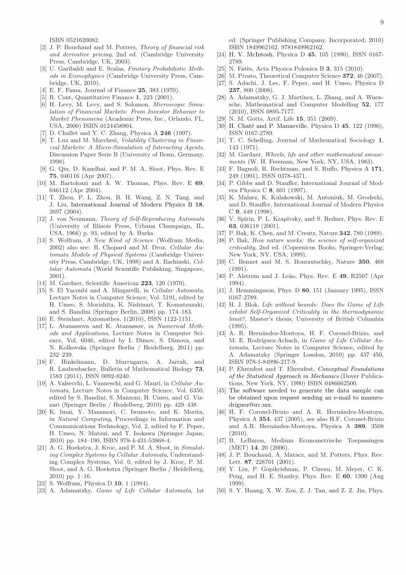
Life evolves on a N ×N two-dimensional lattice withperiodic boundary conditions. We set up a Cartesiancoordinate systemXY centered in the middle point of therectangular lattice, as shown in the left panel of Fig. 1.

We want to describe Life time evolution using the sim-plest but yet comprehensive summary statistics. For thisreason, we select the position of the center of mass con-sidering the alive sites as particles of unitary mass. Giventhe symmetries present in the model we can safely ana-lyze the distance of the center of mass from the origin.Furthermore, we are justified in this choice recalling thatin many cases high-dimensional deterministic dynam-ics is more conveniently described by lower dimensionalstochastic processes, as already noticed by the fathers ofstatistical physics in the second half of XIXth Century[3, 44]. More specifically, to obtain the one-dimensionalobservable analyzed in this paper [45], we construct thevector RCM(i) for each time step i, i = 1, 2, 3, ... as fol-lows:

RCM(i) : = (XCM(i), YCM(i))

=1

N

N∑

x=1

N∑

y=1

Cxy(i)(x, y),

where Cxy(i) denotes the state (1 or 0) of the cell inthe coordinates (x, y) at time step i. The subscript CMstands for center of mass; indeed, RCM(i) is the center ofmass of the living particles at step i (with unitary mass).Fig. 1 (right panel) shows 10000 time steps evolution ofthe vector RCM(i). Our observable ri will be the lengthof RCM(i), i.e. the distance of CM from the origin: ri :=√

XCM(i)2 + YCM(i)2, i = 1, 2, 3, ..,M .In order to analyze this time series, we construct the

returns or logarithmic differences Si for each realizationof the experiment:

Si := log r(i+1) − log r(i), i = 1, 2, 3, ..,M. (1)

Figure 1. Left panel: Coordinate system used to define thevector RCM(i) (the depicted CA state is only for illustrationpurposes). Right panel: an example of the RCM(i) evolution(10000 steps).

We employed a lattice of size N×N = 3000×3000 andthe simulation has been initialized configuring randomlythe 20%, 40%, 60% or the 80% of cells as alive. Thismeans that we have randomly chosen as alive exactly1800000, 3600000, 5400000 or 7200000 of the 9000000total cells.For each one of these densities we generated 20 random

walks of 20000 steps. Considering certain characteristics

3

such as the finite size of the lattice, or a particular ini-tial configuration, generated fluctuations tend to die out(completely dead lattice) or become periodic after an un-known number of time steps. To overcome this problemwe consider only the first 5000 returns of each one of theeighty original samples. The final four time series areobtained by concatenating the similar series, eliminatingthe 19 boundary returns.

III. NUMERICAL RESULTS

Fig. 2a) shows 10 000 time steps of our observable rias a function of time, whereas Fig. 2b) shows the plotof the corresponding log-returns. Both figures were ob-tained from one of the studied time series. Already avisual inspection of the return time series displays anintermittent behavior typical of volatility clustering infinance.

Time step0 2000 4000 6000 8000 10000

r

(i)

0

5

10

15

20

price:time

a)

Time step0 2000 4000 6000 8000 10000

Ret

urn

s S

(i)

-2

-1

0

1

2

rets:time

b)

Figure 2. a) Time evolution ofRCM(i) for a typical realizationof our simulation. b) Corresponding log-returns series.

Return distribution

The empirical densities of standardized returns Si arereported in Fig. 3. Left and right tails are shown inFig. 4. The same figure displays the power-law exponentsobtained by a fit using an optimal cut-off parameter to-gether with the Hill estimator as explained in Ref. [46].Fit parameters are shown in Tab. I and they are consis-tent with a power-law behavior.

Aggregation properties

Although its formation mechanism is not well under-stood, it is well known that financial return distributions

htempEntries 99980

Mean 0.03389RMS 1.022

Returns-30 -20 -10 0 10 20 30

Nu

mb

er o

f E

ntr

ies

1

10

210

310

410

510

htempEntries 99980

Mean 0.03389RMS 1.022

20%40%60%80%

Figure 3. Returns distributions for the four full samples.

Sample α AD Statistic No Cut off20% positive tail 2.79 0.84 441 4.2040% positive tail 3.17 1.38 233 5.8060% positive tail 3.58 0.39 216 5.7080% positive tail 2.38 0.58 235 5.5020% negative tail 3.02 0.49 379 4.5040% negative tail 2.68 1.75 446 4.3060% negative tail 3.20 0.94 222 5.5080% negative tail 2.29 0.29 378 4.20

Table I. Fit parameters from cumulative distribution functiontails, for right and left tails for each of our four standardizedreturn samples. The second column reports estimated powerlaw exponents, the third column Anderson-Darling statistics,the fourth column number of observations fitted in the tailand the last column the chosen cut off value (see Ref. [46]).Only the values in Italics are larger than the critical value atthe 5% significance level.

converge to the normal distribution extremely slowlywhen the time scale increases [5, 47]. This statisticalproperty is called aggregational Gaussianity (or normal-ity) and we want to show its presence in the data.The analysis is performed summing the simple log-

returns of Eq. 1, i.e. considering the following definition

S∆i := log r(i+∆) − log r(i), i = 1, 2, 3, ..,M −∆. (2)

where ∆ stands for the time scale used to aggregate thedata. Here, we underline that the plots in Fig. 5 are ob-tained using overlapping time windows, a method thatis not reliable, but can be used for illustrative purposes.One can see that, as the time scale increases, the em-pirical probability density functions of all four samplesconverge to a normal probability density slowly. Tab. IIand III contain the estimated excess kurtosis and skew-

4

htemp

Entries 99980

Mean -9.072e-05

RMS 1.008

S-110 1 10

1

10

210

310

410

htemp

Entries 99980

Mean -9.072e-05

RMS 1.008

y {x==20}

N

α -1~1.79

a)

htemp

Entries 99980

Mean -0.0003794

RMS 1.01

S-110 1 10

1

10

210

310

410

htemp

Entries 99980

Mean -0.0003794

RMS 1.01

y {x==40}

N

α -1~2.17

b)

htemp

Entries 99980

Mean 0.0002392

RMS 1.009

S-110 1 10

1

10

210

310

410

htemp

Entries 99980

Mean 0.0002392

RMS 1.009

y {x==60}

N

α-1~2.58

c)

htemp

Entries 99980

Mean 0.03389

RMS 1.022

S-110 1 10

1

10

210

310

410

510

htemp

Entries 99980

Mean 0.03389

RMS 1.022

y {x==80}

N

α-1~1.38

d)

htemp

Entries 99980

Mean 9.982e-05

RMS 1.008

S-110 1 10

1

10

210

310

410

htemp

Entries 99980

Mean 9.982e-05

RMS 1.008

z {x==20}

NN

α-1~2.02

e)htemp

Entries 99980

Mean 0.0003794

RMS 1.01

S-110 1 10

1

10

210

310

410 htemp

Entries 99980

Mean 0.0003794

RMS 1.01

z {x==40}

N

α -1~1.68

f)

htemp

Entries 99980

Mean -0.0002392

RMS 1.009

S-110 1 10

1

10

210

310

410

htemp

Entries 99980

Mean -0.0002392

RMS 1.009

z {x==60}

N

α -1~2.20

g)

htemp

Entries 99980

Mean -0.03389

RMS 1.022

S-110 1 10

1

10

210

310

410

510

htemp

Entries 99980

Mean -0.03389

RMS 1.022

z {x==80}

N

α-1~1.29

h)

Figure 4. a) to d) report the right tail distributions of standardized returns. e) to f) report the distributions for left tails.Fit Exponents are also shown in each subfigure. Note: Straight line segments are not fits and are only used for comparisonpurposes.

ness of empirical return distributions for every sampleand for different time scales ∆.

∆ kur20 kur40 kur60 kur801 36.1 41.0 31.9 141.7

10 15.4 18.9 10.6 63.7100 4.5 5.2 3.4 18.5

1000 1.3 1.6 1.1 3.310000 0.97 1.3 0.87 0.57

Table II. Return kurtosis for our four samples and increasingtime scales ∆ used in Fig. 5.

∆ skew20 skew40 skew60 skew80

1 0.08 0.015 -0.02 -0.2910 -0.32 -0.55 -0.03 -1.15

100 -0.06 -0.12 -0.01 -1.091000 0.11 0.05 0.08 -0.202

10000 -0.001 0.005 -0.09 -0.203

Table III. Return skewness for our four samples and increasingtime scales ∆.

From the inspection of Tab. II and III, it turns out that

both skewness and excess kurtosis of return distributionsvanish slowly as the time scale ∆ increases. These empir-ical results are compatible with the convergence of returndistributions to the normal distribution. This analysis isnot sufficient to infer that our data samples satisfies theproperty of aggregational Gaussianity; but the momentbehavior is definitely in agreement with the phenomenon.

Autocorrelation properties

Upper and lower panels of Fig. 6 show the estimatefor the auto-correlation functions (ACF) of returns andof absolute returns, respectively. It can be seen that theACF for returns shows no memory, immediately decay-ing to the level of noise; indeed, Fig. 6 looks similar tothe ACF of daily financial returns. On the other hand,the ACF of absolute returns decays slowly, showing longrange-memory. Both these results are in agreement withthe stylized facts found in financial data. Fig. 7 displaysthe average ACFs over the 20 realizations of each initialcoverage. Power law fits have been performed on the esti-mated absolute return ACF. Fit parameters can be found

5

htempEntries 99980

Mean -9.072e-05

RMS 1.008

Returns-20 -15 -10 -5 0 5 10 15 201

10

210

310

410

htempEntries 99980

Mean -9.072e-05

RMS 1.008

Nu

mb

er o

f E

ntr

ies

Lag10Lag 1

Lag 1000Lag 100

Lag 10000

Gaussian

htempEntries 99980

Mean -0.0003794

RMS 1.01

Returns-20 -15 -10 -5 0 5 10 15 201

10

210

310

410

htempEntries 99980

Mean -0.0003794

RMS 1.01

x

Nu

mb

er o

f E

ntr

ies

htempEntries 99980Mean 0.0002392RMS 1.009

Returns-20 -15 -10 -5 0 5 10 15 201

10

210

310

410

htempEntries 99980Mean 0.0002392RMS 1.009

xhtemp

Entries 99000Mean -0.0001338RMS 1.006

Nu

mb

er o

f E

ntr

ies

htempEntries 99980

Mean 0.03389RMS 1.022

Returns-30 -20 -10 0 10 20 301

10

210

310

410

510

htempEntries 99980

Mean 0.03389RMS 1.022

x

Nu

mb

er o

f E

ntr

ies

Figure 5. Aggregation of the empirical return distributions. When the time lag increases, the empirical probability densitiesconverge to a normal density. The dashed line is a normal density.

in Tab. IV. From this table, it is possible to see that fitsare excellent for samples 20%, 40% and 80%, and goodfor the 60% sample. Based on the above considerations,we can safely conclude that returns are not correlated,whereas absolute return ACFs decay very slowly, follow-ing a power law. All that stuff is in agreement withfinancial stylized facts.

Sample AD statistic β Remaining Obs.20 % 0.536 2.13 29740 % 0.351 2.46 12360 % 1.408 2.02 12680 % 0.299 2.16 135

Table IV. Power law fit exponent parameters for each one ofthe average absolute returns ACF for 20%, 40%, 60% and80% samples.

Leverage effect

Empirical studies of volatility for financial data haveshown that volatility estimates and returns are negativelycorrelated for positive time lag [5, 48]. Following Ref.[48], we investigate this effect by estimating the leveragecorrelation function as:

L(τ) =〈(S2(i+ τ)S(i)〉

V ar(S(i))2. (3)

The estimates for our four samples are shown in Fig. 9.Weak negative correlations are observed for 20% to 60%initial coverage and no correlations for the 80% sample.The same figure shows that the leverage correlation func-

6

Time lag0 20 40 60 80 100

Ret

urn

s A

CF

-0.4-0.2

00.20.40.60.8

1

acf:lag {lag<100}

Time lag10 210

Ab

solu

te R

etu

rns

AC

F 1

aacf:lag {lag<100}

Figure 6. Upper panel: return ACF (linear scale); LowerPanel: absolute return ACF (logarithmic scale). Both esti-mates are based on 15 realizations of our experiment.

Time Lag10 210

AC

F -110

y:i {i<150}

20% Sample40% Sample

60% Sample

80% Sample

Mean ACF of Absolute returns

Figure 7. Absolute returns ACF for all the four samples

tion can be fitted by an exponential function. We foundno correlation between past volatility and future pricechanges and a weak but clear negative correlation withan exponential time decay between future volatility andpast returns changes:

L(τ) =

−Ce−aτ

0

Fitted parameters for the exponent a for each one of ourfour samples are shown in Tab. V. Therefore, from the

Sample a

20% −0.487± 0.04840% 1.098± 0.16460% −0.958± 0.10980% no leverage effect

Table V. Exponential fit leverage exponent a for each one ofthe overall 20%, 40%, 60% and 80% samples.

Time Lag10 210

Mea

n A

CF

of

Sq

uar

ed R

etu

rns

-110

Mu20:i {i<120}

20% Sample

~ 2.13 β

Time Lag10 210

Mea

n A

CF

of

Sq

uar

ed R

etu

rns

-110

Mu40:i {i<120}

40% Sample

~ 2.46 β

Time Lag10 210

Mea

n A

CF

of

Sq

uar

ed R

etu

rns

-110

Mu60:i {i<120}

60% Sample

~ 2.02 β

Time Lag10 210

Mea

n A

CF

of

Sq

uar

ed R

etu

rns

-210

-110

Mu80:i {i<120}

80% Sample

~ 2.16 β

Figure 8. Absolute return ACF for our four samples in alog-log plot. Power law fit exponents are displayed. Straightlines are used to guide the eye. Fit parameters can be foundin Tab. IV.

analysis of this subsection, we can conclude that at leastthree data sets generated with the lowest initial coverageof living states display a weak leverage effect.

Volatility analysis

Volatility v(t) is calculated [49] by averaging the abso-lute returns over a time window T = n∆t as follows:

v(t) :=1

n

t+n−1∑

t′=t

|S(t′)|, (4)

Here we have set up ∆t = 1 time lag and a window of50 time steps. Fig. 10 displays the volatility for the first3000 time steps of our observable for one of our gener-ated random walks. Volatility distributions for the foursamples are shown in Fig. 11.

The data were analyzed in order to fit a suitable distri-bution based on the full sample values of the volatility. Athree-parameter log-normal distribution closely describesthe behavior of the set of volatility values. The cumula-tive distribution function (CDF) is

F (v) = Φ

(

ln(v − λ)− µ

σ

)

, for v > λ. (5)

where Φ denotes the Laplace integral (or the CDF ofa standard normal random variable) and µ, σ and λ de-note the location, scale and threshold parameters, respec-tively. In performing the fit, the values of the parameterswere found using the maximum likelihood estimates. The

7

Time lag-100 -50 0 50 100 150 200 250 300

Lev

erag

e co

rrel

atio

ns

-20

-15

-10

-5

0

5

10

15lev:lag {lag<300 && lag > -100} / ndf 2χ 1.076e+04 / 5978

Constant 0.08022± 2.782

a 0.04752± -0.4868

a) 20%

Time lag-100 -50 0 50 100 150 200 250 300

Lev

erag

e co

rrel

atio

ns

-50

-40

-30

-20

-10

0

10

20

30

40lev:lag {lag<300 && lag > -100} / ndf 2χ 1.365e+04 / 5978

Constant 0.1876± 3.403

a 0.1637± -1.098

b) 40%

Time lag-100 -50 0 50 100 150 200 250 300

Lev

erag

e co

rrel

atio

ns

-30

-20

-10

0

10

20lev:lag {lag<300 && lag > -100} / ndf 2χ 6995 / 5978

Constant 0.1304± 3.229

a 0.1091± -0.9579

c) 60%

Time lag-100 -50 0 50 100 150 200 250 300

Lev

erag

e co

rrel

atio

ns

-300

-200

-100

0

100

200

300

lev:lag {lag<300 && lag > -100}

d) 80%

Figure 9. Leverage effect. It is not there for the sample with initial density of 80% living cells.

time0 1000 2000 3000 4000 5000 6000 7000 8000

Vo

lati

lity

0

0.5

1

1.5

2

2.5

3

vola:lag

Time window 50 time steps

Figure 10. Volatility for a typical generated random walkwith a time window of 50 time steps.

results are shown in Tab. VI for 20%, 40%, 60% and 80%return samples, together with values of the Kolmogorov-Smirnov (KS) statistic measuring the maximum distancebetween the empirical and the fitted cumulative distri-bution function. In general, the fits appears to be fairlygood; from Fig. 12, it can be seen that the empiricaldistribution function (EDF) (solid) and the fitted cumu-lative distribution function (CDF) (dashed) overlap. It

Volatility-210 -110 1

Nu

mb

er o

f E

ntr

ies

0

2000

4000

6000

8000

10000

12000

14000

16000

18000

htempEntries 99931Mean 0.4624RMS 0.5647vola

htempEntries 99931

Mean 0.563

RMS 0.4598volahtemp

Entries 99931

Mean 0.5356

RMS 0.4736volahtemp

Entries 99931Mean 0.5649RMS 0.4457

vola

20%40%60%80%

Figure 11. Volatility frequency histogram for all the samples.

Sample λ µ σ KS-statistic20% 0.08711 -1.1167 0.8712 0.0136240% 0.08308 -1.2306 0.9496 0.0144660% 0.03108 -0.9190 0.7666 0.0261580% 0.03361 -1.3572 0.9918 0.04072

Table VI. Fit parameter and KS-values for the log-normal fits.

is necessary to remark that no statistical goodness-of-fittest can be carried out given that, by construction, the

8

values of the volatility are not independent as requiredby the tests. In this case, the KS statistic is presentedas a descriptive measure to assess the fit quality. In thiscontext, the three-parameter log-normal distribution wasused as a model to describe the general behavior of thedata.

Figure 12. Complementary cumulative probability distri-bution function (1-CDF) for the four samples. Solid lines:volatility empirical probability distribution function. Dashedlines: fitted curve. Both lines almost overlap for all fits. Weplot and fit the empirical complementary cumulative distri-bution for easier comparison.

IV. DISCUSSION

Since GOL is a Class IV Cellular Automata and ex-hibits the property of criticality, it is not a big surpriseto detect power-law distributions emerging from differentobservables, such as spatial/temporal duration of “activ-ity avalanches”, density of living cells and its fluctuations,etc. [33, 37, 38, 50]. In this paper, we chose the summarystatistics |RCM(i)| physically suited to study spatial com-plexity. In doing so, we assumed a priori that some-how the process of mapping the cell distribution fromeach GOL’s microstate (3000 × 3000 dichotomous statevariables) onto the “Center of Mass”(a single continu-ous variable) would conserve the complexity propertiesof GOL. This assumption turns out to be correct and weobtain the expected and ubiquitous power-law distribu-tion of |RCM(i)| variations as well as other unexpected

statistical emergent properties. Once more, these factsdisplay the high Complexity of GOL and its importancefor Complexity Sciences.To rephrase, in a very simple way, we have shown

how Life’s dynamics is able to generate time series dis-playing most of the statistical properties called styl-ized facts, usually connected with financial market dataand recognized as signs of their complexity. By meansof a very simple geometrical mapping, and using atwo-dimensional cellular automaton, we generated syn-thetic data having increments with fat-tailed distribu-tions, clustered volatility, no autocorrelations, long mem-ory in the autocorrelation of absolute returns, aggrega-tional Gaussianity and leverage effect.We believe the use of our scheme can be of help in

understanding the underlying mechanisms governing theformation of the stylized facts. Of course, Life is not thedirect explanation for the emergence of these statisticalproperties but, given its simplicity, we are confident itcan help to build some convincing analogies in order toshade new light on this difficult and important problem.Moreover, we think researchers in both complex sys-

tems and quantitative finance should be aware of howthey can be easily fooled by all these phenomena. Arepower laws really distinct signs of “anomalies”? Isvolatility clustering a pregnant concept? Is leverage cor-relation so peculiar for a time series without indepen-dent increments? Do we need to think about all thesefacts as pillars of our models or is it more likely they arejust “natural” results of non stationarity and non lineardependencies? At this stage, we do not further spec-ulate on the reported findings that are far from givingan explanation and an interpretation of the phenomena.However, this manuscript can be seen as an example ofhow misleading the direct study of these phenomena canbe; phenomena that are complex not because necessarilyconnected with something complicated, but because wedo not yet have any consistent tool to address them.

ACKNOWLEDGMENTS

We appreciate very useful suggestions from S. Jimenezand H. Olivares. We also thank A. Robles from Mar-ket Activity Flow for his support and very useful discus-sions. This work has been supported by Conacyt-Mexicoand MAE-Italy under grant 146498. Also we thank sup-port by Conacyt-Mexico under grant number 155492.The stay of M. Politi at ICU has been financed by theJapanese Society for the Promotion of Science (grant N.PE09043). Plots and the Analyses have been performedusing ROOT [51].

[1] R. N. Mantegna and H. E. Stanley, An introductionto Econophysics: correlations and complexity in finance

(Cambridge University Press, Cambridge, UK, 2000)

9

ISBN 0521620082.[2] J. P. Bouchaud and M. Potters, Theory of financial risk

and derivative pricing, 2nd ed. (Cambridge UniversityPress, Cambridge, UK, 2003).

[3] U. Garibaldi and E. Scalas, Finitary Probabilistic Meth-ods in Econophysics (Cambridge University Press, Cam-bridge, UK, 2010).

[4] E. F. Fama, Journal of Finance 25, 383 (1970).[5] R. Cont, Quantitative Finance 1, 223 (2001).[6] H. Levy, M. Levy, and S. Solomon, Microscopic Simu-

lation of Financial Markets: From Investor Behavior toMarket Phenomena (Academic Press, Inc., Orlando, FL,USA, 2000) ISBN 0124458904.

[7] D. Challet and Y. C. Zhang, Physica A 246 (1997).[8] T. Lux and M. Marchesi, Volatility Clustering in Finan-

cial Markets: A Micro-Simulation of Interacting Agents,Discussion Paper Serie B (University of Bonn, Germany,1998).

[9] G. Qiu, D. Kandhai, and P. M. A. Sloot, Phys. Rev. E75, 046116 (Apr 2007).

[10] M. Bartolozzi and A. W. Thomas, Phys. Rev. E 69,046112 (Apr 2004).

[11] T. Zhou, P. L. Zhou, B. H. Wang, Z. N. Tang, andJ. Liu, International Journal of Modern Physics B 18,2697 (2004).

[12] J. von Neumann, Theory of Self-Reproducing Automata(University of Illinois Press, Urbana Champaign, IL,USA, 1966) p. 93, edited by A. Burks.

[13] S. Wolfram, A New Kind of Science (Wolfram Media,2002) also see: B. Chopard and M. Droz, Cellular Au-tomata Models of Physical Systems (Cambridge Univer-sity Press, Cambridge, UK, 1998) and A. Ilachinski, Cel-lular Automata (World Scientific Publishing, Singapore,2001).

[14] M. Gardner, Scientific American 223, 120 (1970).[15] S. El Yacoubi and A. Mingarelli, in Cellular Automata,

Lecture Notes in Computer Science, Vol. 5191, edited byH. Umeo, S. Morishita, K. Nishinari, T. Komatsuzaki,and S. Bandini (Springer Berlin, 2008) pp. 174–183.

[16] E. Steinhart, Axiomathes, 1(2010), ISSN 1122-1151.[17] L. Atanassova and K. Atanassov, in Numerical Meth-

ods and Applications, Lecture Notes in Computer Sci-ence, Vol. 6046, edited by I. Dimov, S. Dimova, andN. Kolkovska (Springer Berlin / Heidelberg, 2011) pp.232–239.

[18] F. Hinkelmann, D. Murrugarra, A. Jarrah, andR. Laubenbacher, Bulletin of Mathematical Biology 73,1583 (2011), ISSN 0092-8240.

[19] A. Valsecchi, L. Vanneschi, and G. Mauri, in Cellular Au-tomata, Lecture Notes in Computer Science, Vol. 6350,edited by S. Bandini, S. Manzoni, H. Umeo, and G. Viz-zari (Springer Berlin / Heidelberg, 2010) pp. 429–438.

[20] K. Imai, Y. Masamori, C. Iwamoto, and K. Morita,in Natural Computing, Proceedings in Information andCommunications Technology, Vol. 2, edited by F. Peper,H. Umeo, N. Matsui, and T. Isokawa (Springer Japan,2010) pp. 184–190, ISBN 978-4-431-53868-4.

[21] A. G. Hoekstra, J. Kroc, and P. M. A. Sloot, in Simulat-ing Complex Systems by Cellular Automata, Understand-ing Complex Systems, Vol. 0, edited by J. Kroc, P. M.Sloot, and A. G. Hoekstra (Springer Berlin / Heidelberg,2010) pp. 1–16.

[22] S. Wolfram, Physica D 10, 1 (1984).[23] A. Adamatzky, Game of Life Cellular Automata, 1st

ed. (Springer Publishing Company, Incorporated, 2010)ISBN 1849962162, 9781849962162.

[24] H. V. McIntosh, Physica D 45, 105 (1990), ISSN 0167-2789.

[25] N. Fates, Acta Physica Polonica B 3, 315 (2010).[26] M. Pivato, Theoretical Computer Science 372, 46 (2007).[27] S. Adachi, J. Lee, F. Peper, and H. Umeo, Physica D

237, 800 (2008).[28] A. Adamatzky, G. J. Martınez, L. Zhang, and A. Wuen-

sche, Mathematical and Computer Modelling 52, 177(2010), ISSN 0895-7177.

[29] N. M. Gotts, Artif. Life 15, 351 (2009).[30] H. Chate and P. Manneville, Physica D 45, 122 (1990),

ISSN 0167-2789.[31] T. C. Schelling, Journal of Mathematical Sociology 1,

143 (1971).[32] M. Gardner, Wheels, life and other mathematical amuse-

ments (W. H. Freeman, New York, NY, USA, 1983).[33] F. Bagnoli, R. Rechtman, and S. Ruffo, Physica A 171,

249 (1991), ISSN 0378-4371.[34] P. Gibbs and D. Stauffer, International Journal of Mod-

ern Physics C 8, 601 (1997).[35] K. Malarz, K. Kulakowski, M. Antoniuk, M. Grodecki,

and D. Stauffer, International Journal of Modern PhysicsC 9, 449 (1998).

[36] V. Spirin, P. L. Krapivsky, and S. Redner, Phys. Rev. E63, 036118 (2001).

[37] P. Bak, K. Chen, and M. Creutz, Nature 342, 780 (1989).[38] P. Bak, How nature works: the science of self-organized

criticality, 2nd ed. (Copernicus Books, Springer-Verlag;New York, NY, USA, 1999).

[39] C. Bennet and M. S. Bourzutschky, Nature 350, 468(1991).

[40] P. Alstrøm and J. Leao, Phys. Rev. E 49, R2507 (Apr1994).

[41] J. Hemmingsson, Phys. D 80, 151 (January 1995), ISSN0167-2789.

[42] H. J. Blok, Life without bounds: Does the Game of Lifeexhibit Self-Organized Criticality in the thermodynamiclimit?, Master’s thesis, University of British Columbia(1995).

[43] A. R. Hernandez-Montoya, H. F. Coronel-Brizio, andM. E. Rodrıguez-Achach, in Game of Life Cellular Au-tomata, Lecture Notes in Computer Science, edited byA. Adamatzky (Springer London, 2010) pp. 437–450,ISBN 978-1-84996-217-9.

[44] P. Ehrenfest and T. Ehrenfest, Conceptual Foundationsof the Statistical Approach in Mechanics (Dover Publica-tions, New York, NY, 1990) ISBN 0486662500.

[45] The software needed to generate the data sample canbe obtained upon request sending an e-mail to manuro-driguez@uv.mx.

[46] H. F. Coronel-Brizio and A. R. Hernandez-Montoya,Physica A 354, 437 (2005), see also H.F. Coronel-Brizioand A.R. Hernandez-Montoya, Physica A 389, 3508(2010).

[47] B. LeBaron, Medium Econometrische Toepassingen(MET) 14, 20 (2006).

[48] J. P. Bouchaud, A. Matacz, and M. Potters, Phys. Rev.Lett. 87, 228701 (2001).

[49] Y. Liu, P. Gopikrishnan, P. Cizeau, M. Meyer, C. K.Peng, and H. E. Stanley, Phys. Rev. E 60, 1390 (Aug1999).

[50] S. Y. Huang, X. W. Zou, Z. J. Tan, and Z. Z. Jin, Phys.

10

Rev. E 67, 026107 (Feb 2003).[51] R. Brun and F. Rademakers, Nuclear Instruments and

Methods in Physics Research Section A: Accelerators,Spectrometers, Detectors and Associated Equipment

389, 81 (1997), ISSN 0168-9002, new Computing Tech-niques in Physics Research V.