Cellular Automataand Game Design By Pete Strader

Game and Media Design Procedural

Generation Cellular

Automata Game of Life Simple state

Sheep vs. Wolves Mathematical

Model Orcs V.S. Elves

Future Work Sources

Topic Points

The development process of CG content The world The AI

(characters) The Storyline

Saves time and money

Game and Media Designof Video Games

Used in graphics and AI Fractals

Land Scape Geometry

Purlin Noise Texture

Pseudo-Random Variables

Cellular Automata AI Behavior AKA: Agents, NPC,

or Mobs

Procedural GenerationContent Generated Algorithmically

Generated Examples Geography Vegetation Architecture

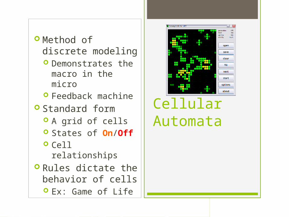
Method of discrete modeling Demonstrates the

macro in the micro Feedback machine

Standard form A grid of cells States of On/Off Cell relationships

Rules dictate the behavior of cells Ex: Game of Life

Cellular Automata

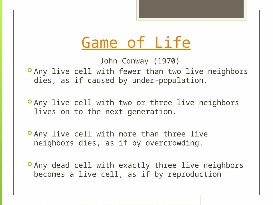
Game of LifeJohn Conway (1970)

Any live cell with fewer than two live neighbors dies, as if caused by under-population.

Any live cell with two or three live neighbors lives on to the next generation.

Any live cell with more than three live neighbors dies, as if by overcrowding.

Any dead cell with exactly three live neighbors becomes a live cell, as if by reproduction

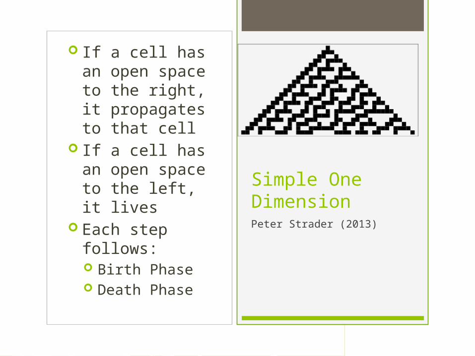
If a cell has an open space to the right, it propagates to that cell

If a cell has an open space to the left, it lives

Each step follows: Birth Phase Death Phase

Simple One DimensionPeter Strader (2013)

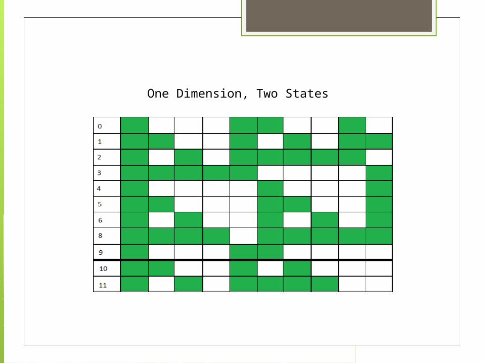
One Dimension, Two States

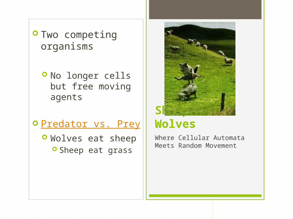
Two competing organisms

No longer cells but free moving agents

Predator vs. Prey Wolves eat sheep

Sheep eat grass

Sheep vs. WolvesWhere Cellular Automata Meets Random Movement

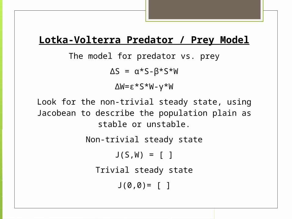
Lotka-Volterra Predator / Prey Model

The model for predator vs. prey

ΔS = α*S-β*S*W

ΔW=ε*S*W-γ*W

Look for the non-trivial steady state, using Jacobean to describe the population plain as stable or unstable.

Non-trivial steady state

J(S,W) = [ ]

Trivial steady state

J(0,0)= [ ]

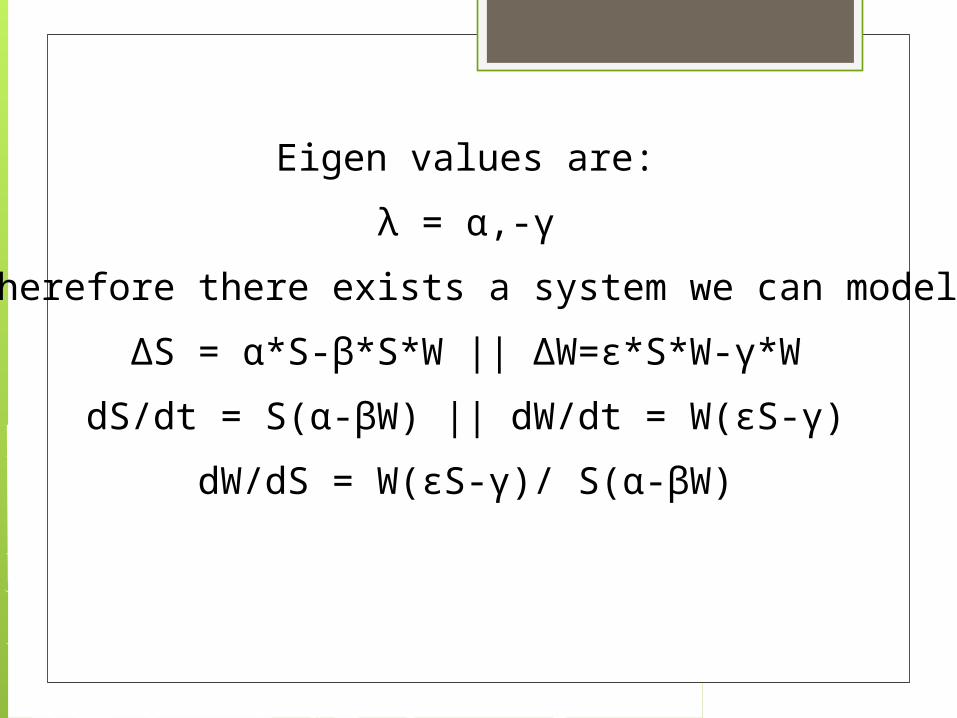
Eigen values are:

λ = α,-γ

Therefore there exists a system we can model

ΔS = α*S-β*S*W || ΔW=ε*S*W-γ*W

dS/dt = S(α-βW) || dW/dt = W(εS-γ)

dW/dS = W(εS-γ)/ S(α-βW)

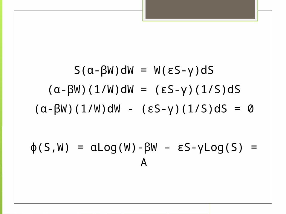
S(α-βW)dW = W(εS-γ)dS

(α-βW)(1/W)dW = (εS-γ)(1/S)dS

(α-βW)(1/W)dW - (εS-γ)(1/S)dS = 0

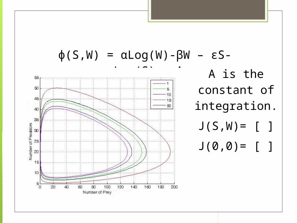
ɸ(S,W) = αLog(W)-βW – εS-γLog(S) = A

ɸ(S,W) = αLog(W)-βW – εS-γLog(S) = A

A is the constant of integration.

J(S,W)= [ ]

J(0,0)= [ ]

Predator vs. Predator

Both eat each other

Stop when stamina is low

Operation Clever Sheep Maniacal laugh …

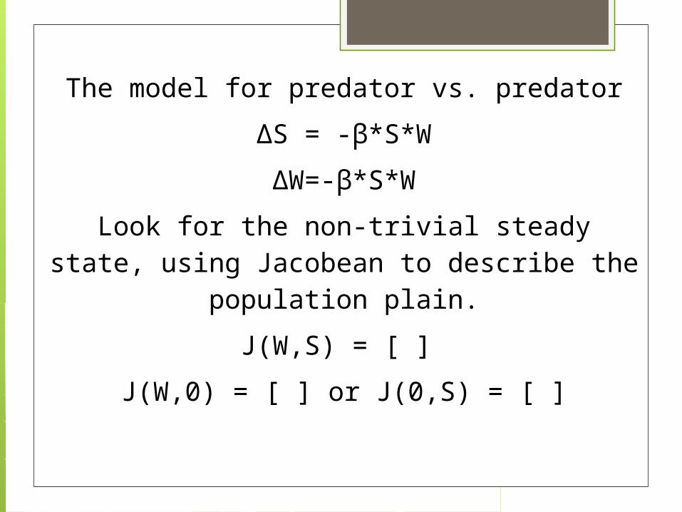
The model for predator vs. predator

ΔS = -β*S*W

ΔW=-β*S*W

Look for the non-trivial steady state, using Jacobean to describe the population plain.

J(W,S) = [ ]

J(W,0) = [ ] or J(0,S) = [ ]

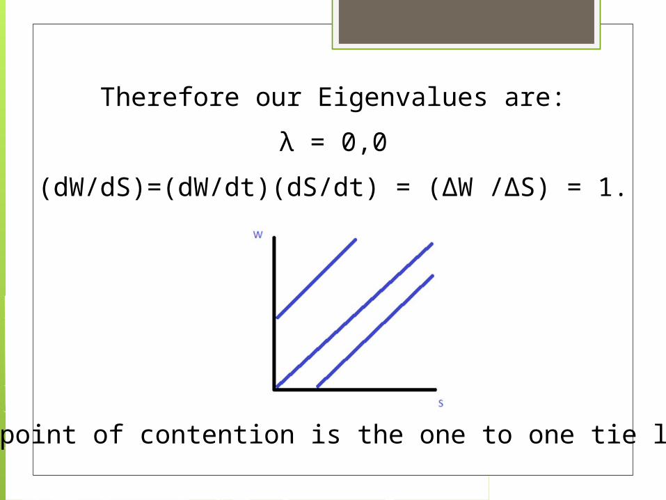
Therefore our Eigenvalues are:

λ = 0,0

(dW/dS)=(dW/dt)(dS/dt) = (ΔW /ΔS) = 1.

Our point of contention is the one to one tie line

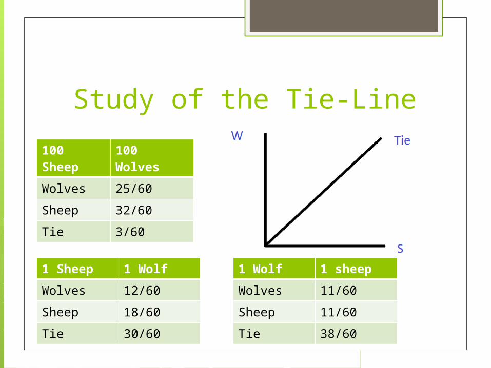
Study of the Tie-Line

100 Sheep

100 Wolves

Wolves 25/60

Sheep 32/60

Tie 3/60

1 Sheep 1 Wolf

Wolves 12/60

Sheep 18/60

Tie 30/60

1 Wolf 1 sheep

Wolves 11/60

Sheep 11/60

Tie 38/60

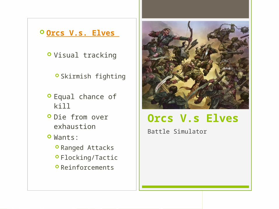
Orcs V.s. Elves

Visual tracking

Skirmish fighting

Equal chance of

kill Die from over

exhaustion Wants:

Ranged Attacks Flocking/Tactic Reinforcements

Orcs V.s Elves Battle Simulator

Expand on code for battle simulator

Add Reinforcements

Study battle outcomes

Add Tactics

Future Work

Sources Nicholas F. Britton, Essential Mathematical

Biology, Springer (2003), pg. 54 Peigen, Jürgens, and Saupe, Chaos and

Fractals, New Frontiers of Science, Springer (1996), pg. 412

NetLogo 5.0.4, (2013) Miguel Cepero, Procedural World,

http://procworld.blogspot.com/ (2013) Massive Software (2013)