Gain scheduled control strategies for a nonlinear

electrostatic microgripper: Design and real time

implementation

Mokrane Boudaoud, Yann Gorrec, Yassine Haddab, Philippe Lutz

To cite this version:

Mokrane Boudaoud, Yann Gorrec, Yassine Haddab, Philippe Lutz. Gain scheduled controlstrategies for a nonlinear electrostatic microgripper: Design and real time implementation.51st IEEE Annual Conference on Decision and Control, CDC’12., Nov 2012, Maui - Hawaii,United States. IEEE 51st Annual Conference on Decision and Control, CDC’12 proceedings,pp.3127-3132, 2012. <hal-01313540>

HAL Id: hal-01313540

https://hal.archives-ouvertes.fr/hal-01313540

Submitted on 10 May 2016

HAL is a multi-disciplinary open accessarchive for the deposit and dissemination of sci-entific research documents, whether they are pub-lished or not. The documents may come fromteaching and research institutions in France orabroad, or from public or private research centers.

L’archive ouverte pluridisciplinaire HAL, estdestinee au depot et a la diffusion de documentsscientifiques de niveau recherche, publies ou non,emanant des etablissements d’enseignement et derecherche francais ou etrangers, des laboratoirespublics ou prives.

Gain scheduled control strategies for a nonlinear electrostaticmicrogripper: Design and real time implementation

Mokrane Boudaoud, Yann Le Gorrec, Yassine Haddab and Philippe Lutz

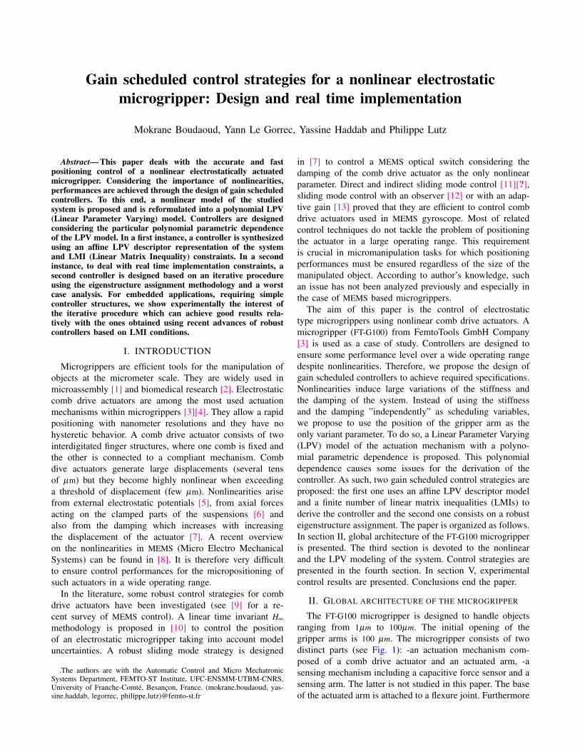
Abstract— This paper deals with the accurate and fastpositioning control of a nonlinear electrostatically actuatedmicrogripper. Considering the importance of nonlinearities,performances are achieved through the design of gain scheduledcontrollers. To this end, a nonlinear model of the studiedsystem is proposed and is reformulated into a polynomial LPV(Linear Parameter Varying) model. Controllers are designedconsidering the particular polynomial parametric dependenceof the LPV model. In a first instance, a controller is synthesizedusing an affine LPV descriptor representation of the systemand LMI (Linear Matrix Inequality) constraints. In a secondinstance, to deal with real time implementation constraints, asecond controller is designed based on an iterative procedureusing the eigenstructure assignment methodology and a worstcase analysis. For embedded applications, requiring simplecontroller structures, we show experimentally the interest ofthe iterative procedure which can achieve good results rela-tively with the ones obtained using recent advances of robustcontrollers based on LMI conditions.

I. INTRODUCTION

Microgrippers are efficient tools for the manipulation ofobjects at the micrometer scale. They are widely used inmicroassembly [1] and biomedical research [2]. Electrostaticcomb drive actuators are among the most used actuationmechanisms within microgrippers [3][4]. They allow a rapidpositioning with nanometer resolutions and they have nohysteretic behavior. A comb drive actuator consists of twointerdigitated finger structures, where one comb is fixed andthe other is connected to a compliant mechanism. Combdive actuators generate large displacements (several tensof µm) but they become highly nonlinear when exceedinga threshold of displacement (few µm). Nonlinearities arisefrom external electrostatic potentials [5], from axial forcesacting on the clamped parts of the suspensions [6] andalso from the damping which increases with increasingthe displacement of the actuator [7]. A recent overviewon the nonlinearities in MEMS (Micro Electro MechanicalSystems) can be found in [8]. It is therefore very difficultto ensure control performances for the micropositioning ofsuch actuators in a wide operating range.

In the literature, some robust control strategies for combdrive actuators have been investigated (see [9] for a re-cent survey of MEMS control). A linear time invariant H∞

methodology is proposed in [10] to control the positionof an electrostatic microgripper taking into account modeluncertainties. A robust sliding mode strategy is designed

.The authors are with the Automatic Control and Micro MechatronicSystems Department, FEMTO-ST Institute, UFC-ENSMM-UTBM-CNRS,University of Franche-Comte, Besancon, France. (mokrane.boudaoud, yas-sine.haddab, legorrec, philippe.lutz)@femto-st.fr

in [7] to control a MEMS optical switch considering thedamping of the comb drive actuator as the only nonlinearparameter. Direct and indirect sliding mode control [11][?],sliding mode control with an observer [12] or with an adap-tive gain [13] proved that they are efficient to control combdrive actuators used in MEMS gyroscope. Most of relatedcontrol techniques do not tackle the problem of positioningthe actuator in a large operating range. This requirementis crucial in micromanipulation tasks for which positioningperformances must be ensured regardless of the size of themanipulated object. According to author’s knowledge, suchan issue has not been analyzed previously and especially inthe case of MEMS based microgrippers.

The aim of this paper is the control of electrostatictype microgrippers using nonlinear comb drive actuators. Amicrogripper (FT-G100) from FemtoTools GmbH Company[3] is used as a case of study. Controllers are designed toensure some performance level over a wide operating rangedespite nonlinearities. Therefore, we propose the design ofgain scheduled controllers to achieve required specifications.Nonlinearities induce large variations of the stiffness andthe damping of the system. Instead of using the stiffnessand the damping ”independently” as scheduling variables,we propose to use the position of the gripper arm as theonly variant parameter. To do so, a Linear Parameter Varying(LPV) model of the actuation mechanism with a polyno-mial parametric dependence is proposed. This polynomialdependence causes some issues for the derivation of thecontroller. As such, two gain scheduled control strategies areproposed: the first one uses an affine LPV descriptor modeland a finite number of linear matrix inequalities (LMIs) toderive the controller and the second one consists on a robusteigenstructure assignment. The paper is organized as follows.In section II, global architecture of the FT-G100 microgripperis presented. The third section is devoted to the nonlinearand the LPV modeling of the system. Control strategies arepresented in the fourth section. In section V, experimentalcontrol results are presented. Conclusions end the paper.

II. GLOBAL ARCHITECTURE OF THE MICROGRIPPER

The FT-G100 microgripper is designed to handle objectsranging from 1µm to 100µm. The initial opening of thegripper arms is 100 µm. The microgripper consists of twodistinct parts (see Fig. 1): -an actuation mechanism com-posed of a comb drive actuator and an actuated arm, -asensing mechanism including a capacitive force sensor and asensing arm. The latter is not studied in this paper. The baseof the actuated arm is attached to a flexure joint. Furthermore

a suspension mechanism including two pairs of clamped-clamped beams holds the movable part of the actuator.

Fig. 1. Structure of the FT-G100 microgripper (FemtoTools GmbH).

III. MODELING OF THE ACTUATION MECHANISM

A. Nonlinear dynamic modeling

The dynamic model of the actuation mechanism is basedon the nonlinear Duffing equation which takes into accountaxial forces ~N acting on the clamped parts of the suspensions(Fig. 2a). Such forces are considered by introducing a cubicstiffness ka3 in the dynamic equation [8]. In the case of themicrogripper, the Duffing equation is given as:

ma.d2ya(L)

dt2 +da.dya(L)

dt+ ka1.ya(L)+ ka3.y3

a(L) =1

Da.Felec (1)

ma, da and ka1 are respectivelythe linear mass, the lineardamping and the linear stiffness of the actuation mechanisms,Da is an amplification factor.

N

Felec

L

xea

Ls

Hinge joint

ya (xea)

ya(L)

Vin

Actuated arm

(a)

Laser sensor

Shuttle

L

xea

Hinge joint

ya(L)

Actuated arm

x

y z

mass

stiffness

damping

(b)

ya (xea) Vin

Fig. 2. Simplified scheme of the FT-G100 actuation mechanism (a) andequivalent scheme of suspension mechanism (b).

The electrostatic force Felec generated by the comb driveactuator is defined as:

Felec =Na.ε.hz

2.g.V 2

in (2)

Where, Na = 1300 is the number of comb fingers, ε =

8.85pF/m is the permittivity of the air, hz = 50µm is thethickness of comb fingers, and g = 6µm is the gap spacingbetween two fingers. Under the assumption that the base ofthe actuated arm behaves as a hinge joint (Fig. 2) and that theactuated arm is rigid, the amplification mechanism is givenas: Da =

Lxea

, with L = 5150µm and xea = 1100µm.

A laser interferometer sensor (SP-120 SIOS MetechnikGmbH) is used to derive the experimental static charac-teristic ya(L)/Vin from 0 to 200V . Experimental data arethen fitted using equation (1) in static mode. With a thirdorder polynomial interpolation, the mean fitting of the staticcharacteristic is found to be equal to 17.11 %. To reduce thiserror, we have extended the Duffing equation by consideringa sixth order polynomial in the static characteristic leading

to the following expression:6∑

i=1kai.yi

a(L) =Na.ε.hz2.g.Da

.V 2in. This

polynomial extension allows taking into account additionalnonlinearities that are not considered in the standard Duffingequation. Therefore, by fitting experimental data with theextended Duffing static equation, the mean error is reducedto 3.66 % and results are presented in Fig. 3a.

0 50 100 150 2000

20

40

60

80

100

Actuation voltage (Volts)A

ctua

ted

arm

tip

dis

plac

emen

t (µ

m)

ModelExperimental data

(a)

0 20 40 60 80 1001

1.5

2

2.5

3

3.5

4

4.5

Actuated arm tip displacement (µm)

Stif

fnes

s (N

/m)

ModelExperimental data

(b)

0 20 40 60 80 1000

1

2

3

4

5x 10-5

Actuated arm tip displacement (µm)

Dam

ping

(N

s/m

)

ModelExperimental data

(c)

Fig. 3. Nonlinear characteristics of the FT-G100 actuation mechanism (a)static actuated arm tip displacement/ supply voltage, (b) stiffness/actuatedarm tip displacement, (c) damping/actuated arm tip displacement.

Identified parameters are given as: ka1 = 1,0762N/m,ka2 = −1,6× 103N/m2, ka3 = 4,88× 108N/m3, ka4 = −1,69×1012N/m4, ka5 = −3,98× 1016N/m5, ka6 = 4,71× 1020N/m6.Consequently, the nonlinear evolution of the stiffness in theactuation mechanism is deduced as shown in Fig. 3b.

To identify the mass and the damping, step excitationsare applied to the actuator in the operating range 0 to200V and the displacements ya(L) are measured with thelaser sensor. It is observed that the damping of the systemincreases with increasing the amplitude of motion startingfrom ya(L) = 60µm. A nonlinear damping term of the form

da(ya(L)) =4∑

i=0dai.yi

a(L) is then introduced in (1). A fourth

order polynomial has been sufficient to describe the non-linear damping (Fig. 3c). The mass is identified with theexperimental step response of the actuation mechanism for5V input voltage. Moreover, the damping is identified at eachoperating point from experimental step responses and resultsare fitted on the fourth order polynomial. Identified parame-ters are: ma = 3,9843×10−8Kg, da0 = 3,01×10−6Ns/m, da1 =

−0,162Ns/m2, da2 = 1,24×104Ns/m3, da3 =−3,04×108Ns/m4,da4 = 2,47×1012Ns/m5.

Taking into acoount the nonlinear stiffness and damping,we obtain the following nonlinear state space model:

[ya(L)ya(L)

]=

0 1

− 1ma

6∑

i=1kaiyi−1

a (L) − 1ma

4∑

i=0daiyi

a(L)

[ya(L)ya(L)

]

+

0Na.ε.hz

2.g.Da

.V 2in

ya(L) =[

1 0][ya(L)

ya(L)

](3)

For the model validation, the experimental frequencyspectrum of the system is compared with the simulated oneusing (3) and a good agreement is observed Fig. 4. Thefirst resonance frequency varies from 827Hz to about 2KHz.Moreover three vibration modes appear staring from Vin=50V. Such characteristics are well captured in the nonlinearmodel. For control purposes, the model (3) is reformulatedinto a LPV model in such a way that the position of theactuated arm tip is the only variant parameter.

Fig. 4. Frequency responses of the nonlinear actuation mechanism:experimental data (red curve) and simulation data (black curve)

B. LPV modeling

The nonlinear model (3) can be reformulated into an affineLPV model if the damping and the stiffness are chosenindependently as varying parameters Fig. 2b. For this classof LPV models, well known gain scheduled control strategiessuch as LPV/H∞ [14] can be used. The main drawback of thisapproach is that the polynomial dependence of the nonlinearparameters is not taken into account during the controllerdesign leading to a high conservatism. In the present work,we propose to use the operating point (actually the positionof the actuated arm tip) as the only varying parameter. Tothis end, using a Jacobian linearization, the nonlinear plant(3) is formulated into a polynomial LPV model of the form:{

Xp(t) = Ap(δ )Xp(t)+Bp.U(t)ya(L, t) =CpXp(t)

(4)

Ap(δ ) =

0 1

− 1ma

.6∑

i=1i.kai.δ

i−1 − 1ma

.4∑

i=0dai.δ

i

Bp =

[0 Na.ε.hz

2.g.Da

]T,Cp = [ 1 0 ],Xp =

[ya(L)˙ya(L)

]Ap ∈ Rn×n,Bp ∈ Rn×m,Cp ∈ Rp×n with n = 2, p = m = 1.

ya(L) is the variation of ya(L) around an operating point δ . Tosimplify notations, the variable ya(L) will be designed laterby ya. Note that, the nonlinearity arising from square inputvoltage is overcome by considering the variable U = V 2

in asthe model input in the control design.

The polynomial parametric dependence of the LPV model(4) causes some issues for the derivation of a gain scheduledcontroller. To overcome this control design issue, two strate-gies are suggested in the next section.

IV. GAIN SCHEDULED CONTROL STRATEGIES

To design a parameter dependant controller for which thescheduled parameter is the operating point δ , two distinctapproaches are proposed: 1) To transform the polynomialLPV model into an affine LPV descriptor model and todesign a controller with the resolution of a finite numberof LMIs. 2) To perform an iterative procedure based on aworst case analysis and an eigenstructure assignment usingobserved based scheduled controller. Both methods finallyallow designing a parameter dependant controller taking intoaccount the particular polynomial form of (4).

A. Affine LPV descriptor representation and gain scheduledcontrol synthesis

For the derivation of an affine LPV descriptor model ofthe system, starting from (4), we have performed a linearfractional transformation Fig. 5 of the form: Xp

ya

z

=

N11 N12 N13N21 N22 N23N31 N32 N33

Xp

Uv

(5)

With: v(t) = δ z(t), z(t) ∈ Rnz , v(t) ∈ Rnv .The sub-matrices

{Ni, j}

i, j=1,...,3 are deduced from theinterconnexion of the LFT. Taking into account the stiffnessand damping polynomial orders, we have selected nz = nv = 7(e.i. order of the highest polynomial +1).

The affine LPV model (6) is obtained by defining anaugmented state vector Xdes =

[XT

p vT ]T such as:{EXdes = Ades(δ )Xdes +BdesUya =CdesXdes

(6)

Ades =

[N11 N13

δN31 δN33 + Inv

]Bdes =

[N12δN32

]Cdes =

[Cp 01×nv

]E = diag(In,0nv)

This descriptor representation is used only to derive thegain scheduled controller via the resolution of a finite numberof LMIs conditions. Control performances required in thisstudy are derived from general need in micromanipulation:no overshoot, maximum static error lower than 0.05%. More-over, we desire obtain a maximal response time lower than30ms. Therefore, we have defined a reference closed looptransfer function Td :

Td =0.9995

4×10 - 6s2 +0.006 s + 1(7)

The reference model Td contains two eigenvalues λ1 =

−191 and λ2 =−1300. In order to design the gain scheduled

controller that ensure desired performances in wide operatingrange, a weighting transfer function W1(s) is introduced.

This function will allow tracking performances by apply-ing specifications to the sensitivity function of the systemconsidering a frozen value of δ . In this study we haveselected the frozen value as the steady tip displacement of theactuated arm for 5V input voltage. The weighting function isgiven by W1(s) = 1

1−Td. Therefore, the descriptor model (6) is

augmented with the weighting function leading to:EgXg = Ag(δ )Xg +B1w+B2Uz =C1Xg +D11wya =C2Xg +D21w

(8)

The external input w = yar is the trajectory reference andthe external output z1 is the output of W1(s).

The control problem consists in designing a gain scheduledcontroller K(s,δ ) that minimize a positive scalar γ such asthe closed loop transfer H∞ norm of the performance channelw→ z1 is minimized (ideally less or equal to 1) for any valueof the operating point δ . Such requirement can be satisfiedby solving the following LMI constraints [15]:[

Y ETg Eg

ETg ET

g χ

]=

[Y ET

g EgET

g ETg χ

]T

> 0 MA +MTA MB MT

CMT

B −γI MTD

MC MD −γI

< 0

(9)

MA =

[Ag(δ )Y T +B2FT Ag(δ )

HT χT Ag(δ )+GTC2

]

MB =

[B1

χT B1 +GT D21

]Mc =

[C1Y T +D12FT C1

]The decision variables of (9) are the matrices χ, Y , F , G

and H with a appropriate dimensions.As, the varying parameter is bounded between upper (δM)

and lower (δm) values, the LMI problem results in an infiniteset of LMIs to solve. Nevertheless, since the matrix Ag(δ ) isaffine w.r.t the varying parameter, the LMIs (9) can be solvedonly on the vertices [16] of the set [δm δM ]. Here only two setsof LMIs must be solved since only one varying parameteris considered. If this is feasible, the solution leads to thefollowing polytopic state space controller structure:

K(s,δ ) = α1(δ )

[Ak1 Bk1Ck1 0

]+α2(δ )

[Ak2 Bk2Ck2 0

](10)

The matrices {Aki,Bki,Cki} are derived from the solution ofthe LMIs (9) and {α1(δ ),α2(δ )} are given by α1(δ ) =

δM−δ

δM−δmand α2(δ ) = 1−α1(δ ).

The augmented LPV descriptor model (8), is transformedinto a polytopic LPV model with two vertices. Thereafter,the LMIs conditions (9) are solved at each vertex of themodel using the Matlab LMI Control Toolbox. For theresolution, we have considered δm = 1µm and δM = 90µm.Consequently, two four order controllers Gk1 {Ak1,Bk1,Ck1,0}and Gk2 {Ak2,Bk2,Ck2,0} are obtained. Experimental control

results using this strategy are presented in section V. Nev-ertheless, due to the order of the obtained controller, somereal time implementations constraints have been encountered.The second proposed control strategy aim at overcoming thisconstraint while keeping desired performances.

pX pXɺ

ay

∫

v z

Polynomial LPV

model

δ

U K(s,δ)

W1

w=yar + _

Linear fractional transformation

z1

Fig. 5. Control scheme with the augmented LPV descriptor model.

B. Gain scheduled control by eigenstructure assignment

The strategy proposed in this section is based on theoutput feedback control by eigenstructure assignment andmulti model self scheduled control design [18]. It is wellknown that with the traditional eigenstructure assignment[17], the maximal number of eigenvalues that can be assignedis limited by the number of outputs of the controlled system.First, let us consider the LPV polynomial model (4) fora given frozen value δ0. This model has one output andthe reference model contains two eigenvalues. Thereforeto assign the eigenvalues of the frozen parameter systemconsidering the reference model (7), we propose to add anobserver to the polynomial LPV model based on Lemma 1.Lemma 1: the system defined by (see Fig. 6 ){

zo = πozo− toya +uoBpUuoAp(δ0)+ toCp = πouo

(11)

uo ∈Cn, to ∈Cp,πo ∈Cis an observer of the variable zo = πoXp and the observationerror εo = zo− uoXp satisfies: εo = πoεo (see [19]). Note thatδ0 is a frozen value of the varying parameter δ .

Polynomial LPV model to ∫

πo uoBp

U zo _

+ + +

ya

Fig. 6. Elementary observer of zo = πoXp

Designing an output feedback controller by eigenstructureassignment to the frozen polynomial LPV model (4) with theobserver consists on finding the matrix Kc = [Ky Kz] such asthe system:

Xp = Ap(δ0)Xp +BpUzo = πozo +uoBpU− toya

ya =CpXp

(12)

controlled by U = Kyya + Kzzo have the expected perfor-mances. This problem can be resolved by considering theseparation principle described in the theorem 1 [20].

Theorem 1: It is equivalent to assign (by the static feedbackKc = [Ky Kz]) the eigenvalues of the system (12) and the oneof the system (13).

Xp = Ap(δ0)Xp +BpU[ya

zo

]=CpoXp

(13)

Where: Cpo = [CTp uT

o ]T

The gains Ky and Kz allow the assignment of the eigenval-ues λ1 and λ2 respectively. On the other hand, to ensure astatistic error lower than 0.05%, we have added an integratoron the signal yar− ya (recall that yar is the reference trajec-tory). In this case, the matrix Kc is extended to Kc = [Ky Kz Ki]

and the control low becomes U = Ki∫

ε−Kyya−Kzzo, whereε = yar−ya. The gain Ki is used to assign a third eigenvalue.

-4000 -3000 -2000 -1000 0-1

-0.5

0

0.5

1x 104

Real

Imag

inar

y

(a)

Reference model

Worst case model

Set of elementarymodels

***

-6000 -4000 -2000 0 2000-500

0

500

Real

Imag

inar

y

**

*

(b)

Reference model

Worst case model

Set of elementarymodels

-3500 -3000 -2500 -2000 -1500 -1000 -500 0-1

-0.5

0

0.5

1

Real

Imag

inar

y

**

* Reference model

Worst case model

Set of elementary models

(c)

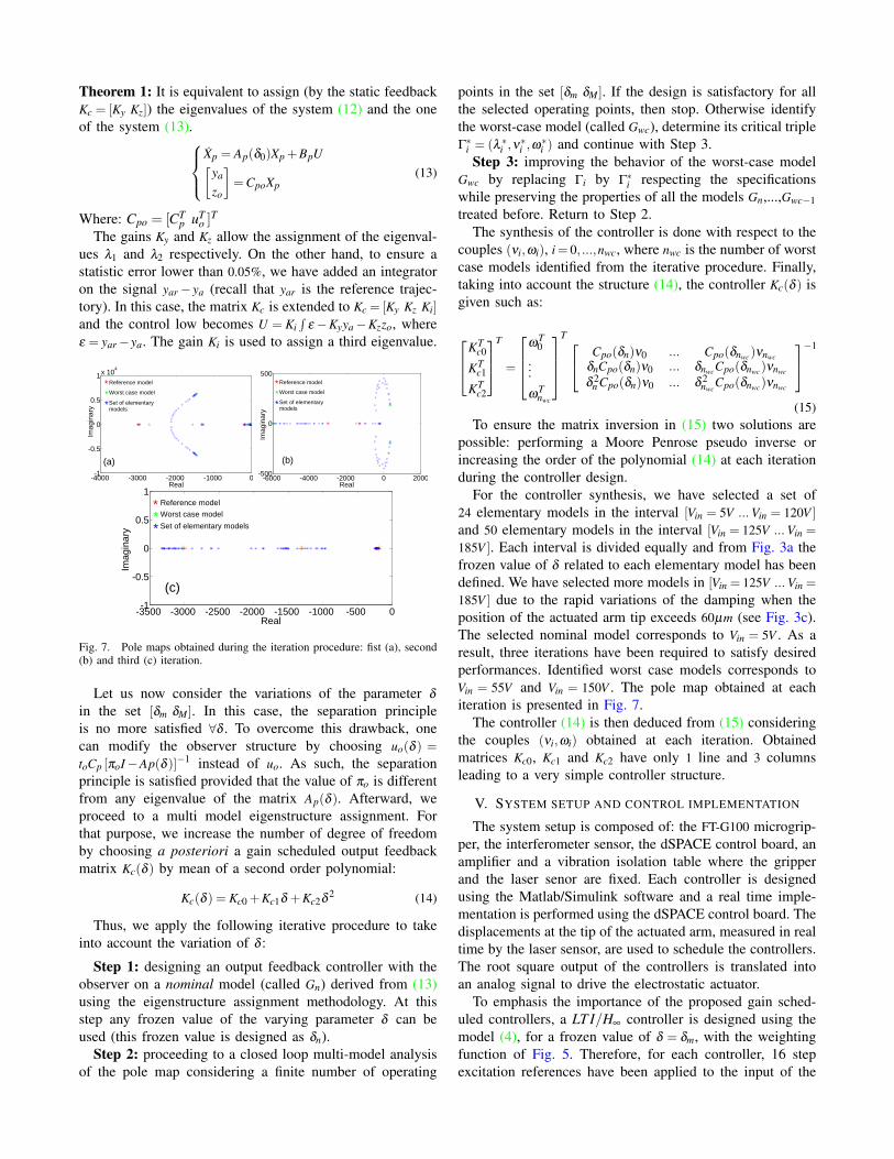
Fig. 7. Pole maps obtained during the iteration procedure: fist (a), second(b) and third (c) iteration.

Let us now consider the variations of the parameter δ

in the set [δm δM ]. In this case, the separation principleis no more satisfied ∀δ . To overcome this drawback, onecan modify the observer structure by choosing uo(δ ) =

toCp [πoI−Ap(δ )]−1 instead of uo. As such, the separationprinciple is satisfied provided that the value of πo is differentfrom any eigenvalue of the matrix Ap(δ ). Afterward, weproceed to a multi model eigenstructure assignment. Forthat purpose, we increase the number of degree of freedomby choosing a posteriori a gain scheduled output feedbackmatrix Kc(δ ) by mean of a second order polynomial:

Kc(δ ) = Kc0 +Kc1δ +Kc2δ2 (14)

Thus, we apply the following iterative procedure to takeinto account the variation of δ :

Step 1: designing an output feedback controller with theobserver on a nominal model (called Gn) derived from (13)using the eigenstructure assignment methodology. At thisstep any frozen value of the varying parameter δ can beused (this frozen value is designed as δn).

Step 2: proceeding to a closed loop multi-model analysisof the pole map considering a finite number of operating

points in the set [δm δM ]. If the design is satisfactory for allthe selected operating points, then stop. Otherwise identifythe worst-case model (called Gwc), determine its critical tripleΓ∗i = (λ ∗i ,ν

∗i ,ω

∗i ) and continue with Step 3.

Step 3: improving the behavior of the worst-case modelGwc by replacing Γi by Γ∗i respecting the specificationswhile preserving the properties of all the models Gn,...,Gwc−1treated before. Return to Step 2.

The synthesis of the controller is done with respect to thecouples (νi,ωi), i= 0, ...,nwc, where nwc is the number of worstcase models identified from the iterative procedure. Finally,taking into account the structure (14), the controller Kc(δ ) isgiven such as:

KTc0

KTc1

KTc2

T

=

ω

T0

...

ωTnwc

T Cpo(δn)ν0 ... Cpo(δnwc)νnwc

δnCpo(δn)ν0 ... δnwcCpo(δnwc)νnwc

δ 2n Cpo(δn)ν0 ... δ 2

nwcCpo(δnwc)νnwc

−1

(15)To ensure the matrix inversion in (15) two solutions are

possible: performing a Moore Penrose pseudo inverse orincreasing the order of the polynomial (14) at each iterationduring the controller design.

For the controller synthesis, we have selected a set of24 elementary models in the interval [Vin = 5V ...Vin = 120V ]

and 50 elementary models in the interval [Vin = 125V ...Vin =

185V ]. Each interval is divided equally and from Fig. 3a thefrozen value of δ related to each elementary model has beendefined. We have selected more models in [Vin = 125V ...Vin =

185V ] due to the rapid variations of the damping when theposition of the actuated arm tip exceeds 60µm (see Fig. 3c).The selected nominal model corresponds to Vin = 5V . As aresult, three iterations have been required to satisfy desiredperformances. Identified worst case models corresponds toVin = 55V and Vin = 150V . The pole map obtained at eachiteration is presented in Fig. 7.

The controller (14) is then deduced from (15) consideringthe couples (νi,ωi) obtained at each iteration. Obtainedmatrices Kc0, Kc1 and Kc2 have only 1 line and 3 columnsleading to a very simple controller structure.

V. SYSTEM SETUP AND CONTROL IMPLEMENTATION

The system setup is composed of: the FT-G100 microgrip-per, the interferometer sensor, the dSPACE control board, anamplifier and a vibration isolation table where the gripperand the laser senor are fixed. Each controller is designedusing the Matlab/Simulink software and a real time imple-mentation is performed using the dSPACE control board. Thedisplacements at the tip of the actuated arm, measured in realtime by the laser sensor, are used to schedule the controllers.The root square output of the controllers is translated intoan analog signal to drive the electrostatic actuator.

To emphasis the importance of the proposed gain sched-uled controllers, a LT I/H∞ controller is designed using themodel (4), for a frozen value of δ = δm, with the weightingfunction of Fig. 5. Therefore, for each controller, 16 stepexcitation references have been applied to the input of the

0 0.05 0.1 0.150

0.2

0.4

0.6

0.8

1

Time (s)

Nor

mal

ized

con

trol

led

posi

tion

(a)

0 0.005 0.01 0.015 0.02 0.025 0.03 0.035 0.04 0.045 0.050

0.2

0.4

0.6

0.8

1

Time (s)

Nor

mal

ized

con

trol

led

posi

tion

(b)

0 0.005 0.01 0.015 0.02 0.025 0.03 0.035 0.04 0.045 0.050

0.2

0.4

0.6

0.8

1

Time (s)

Nor

mal

ized

con

trol

led

posi

tion

(c)

Fig. 8. Experimental step responses of the controlled microgripper atdifferent operating points (from 5µm to 90µm actuated arm tip displace-ment). The black curve refer to the step response of the reference modelTd . Controllers are defined as: a) method 1, b) method 2, c) method 3

closed loop system. The amplitude of the step excitationsvaries from 5µm to 90µm with a step of 5µm. Results of thecontrolled displacements normalized to unity (divided by theinput reference) of the actuated arm tip in response to thestep excitations are presented in (8). We have referred tomethod 1, method 2 and method 3, the LT I/H∞ controller,the controller obtained by the descriptor model, and thecontroller based on the iterative procedure respectively.

It is clear from Fig. 8 that the LT I/H∞ controller cannotguarantee the required performances when performing largedisplacements of the actuator. Performances are respectedover the operating range 5µm < δ < 90µm with the method2 and the method 3. The latter allows obtaining the desiredresponse time, no overshoot is observed and the static error isless than 0.05%. This demonstrated and justify the proposedgain scheduled controllers w.r.t the parameter δ for thecontrol of the comb drive actuator for large displacements.

Some real time implementation constraints have beenencontourned for the controller based on the methods 2. Dueto the high order of the controller (two transfer functions witha fourth order denominator), the sampling frequency of thedSPACE control board had to be reduced to 15KHz for anefficient implementation while with the very simple structureof the controller based on method 3, the implementationcould be performed easily until 100KHz sampling frequency.This demonstrates the interest of the method 3 for real timeimplementations constraints. Such a requirement is moreand more needed for embedded applications in the field ofrobotics micromanipulation. A solution to use the method2 for embedded application is to reduce the order of thecontroller. Nevertheless, controller reductions can lead to aloss of performances.

VI. CONCLUSIONS

This paper has dealt with the gain scheduled control ofa nonlinear electrostatic microgripper. A nonlinear dynamicmodel of the actuation mechanisms has been proposed andmain nonlinear parameters have been identified experimen-tally. For control purposes, the nonlinear model is reformu-lated into a polynomial LPV model. To deal with the partic-ular structure of the LPV model, two gains scheduled controlstrategies are proposed and experimental implementationresults are presented. The interest of the iterative procedurefor the control of comb drive actuators over large dis-placements in embedded applications is demonstrated withexperimental arguments. The latter can achieve good resultsrelatively with the ones obtained using recent advances ofrobust controllers based on LMIs conditions. Future workswill concern the implementation of the controller based onthe iterative procedure in micro-calculators such as FPGA.Therefore, high control performances can be achieved duringa micromanipulation processes without the use of a highperformance controller board such as dSPACE.

REFERENCES

[1] B. Tamadazte, E. Marchand, S. Dembele, N Le Fort-Piat, ”CAD modelbased tracking and 3D visual-based control for MEMS microassem-bly”, Int J of Robotics Research, vol. 29, pp. 1416-1437, 2010.

[2] X Y. Liu, K Y. Kim, Y. Zhang, Y. Sun, ”Nanonewton force sensing andcontrol in microrobotic cell manipulation”, Int J of Robotics Research,vol.28, pp.1065-1076, 2009.

[3] F. Beyeler, A. Neild, S. Oberti, D. Bell, S. Yu, J. Dual, B. Nelson,”Monolithically fabricated microgripper with integrated force sensorfor manipulating microobjects and biological cells aligned in anultrasonic field”, JMEMS, vol.16, pp.7-15, 2007.

[4] K. Kim, L. Xinyu, Z. Yong, Y. Sun, ”Nanonewton force-controlled ma-nipulation of biological cells using a monolithic MEMS microgripperwith two-axis force feedback”, J. Micromech. Microeng, vol.8, 2008.

[5] K B. Lee, A P. Pisano, L. Lin, ”Nonlinear behaviors of a comb driveactuator under electrically induced tensile and compressive stresses”,J.M.M, vol.17, pp.55756, 2007.

[6] R. Legtenberg, A. Groeneveld, M. Elwenspoek, ”Combdrive actuatorsfor large displacements”, J.M.M, vol.6, pp.320-329,1996.

[7] B. Ebrahimi, M. Bahrami, ”Robust sliding-mode control of a MEMSoptical switch”, Journal of Physics, vol.34, pp.728733, 2006.

[8] R. Lifshitz, M C. Cross, ”Nonlinear Dynamics of Nanomechanicaland Micromechanical Resonators”, Review of Nonlinear Dynamicsand Complexity, Edited by Heinz Georg Schuster, Wiley, 2008.

[9] A. Ferreira, S S. Aphale, ”A Survey of Modeling and ControlTechniques for Micro- and Nanoelectromechanical Systems”, IEEETransactions on Systems, Man, and Cybernetics, Part C: Applicationsand Reviews, vol.41, pp.350-364, 2011.

[10] Y. Haddab, B. Uccheddu, ”Commande robuste d’une pince microfab-rique actionnement lectrostatique”, Conference Internationale Fran-cophone d’Automatique CIFA 2010, Bucarest, Romania, 2008. (inFrench).

[11] A. Kuzu, ”Control Strategies for Increased Reliability in MEM CombDrives”, Proceedings of the 2nd WSEAS Int. Conference on Appliedand Theoretical Mechanics, Venice, Italy, 2006.

[12] J. Fei, C. Batur, ”Adaptive sliding mode control with sliding mode ob-server design for a MEMS vibratory gyroscope”, ASME InternationalMechanical Engineering Congress and Exposition, 2007.

[13] J. Fei, C. Batur, ”A class of adaptive sliding mode controller withproportional-integral sliding surface”, journal of system and controlengeneering, vol.223, pp.989-999, 2009.

[14] A. Zin, O. Sename, P. Gaspar, L. Dugard, J. Bokor, ”An LPV/HinfActive Suspension Control for Global Chassis Technology: Designand Performance Analysis”, IEEE American Control Conference,Minneapolis, USA, 2006

[15] I. Masubuchi, J. Kato, M. Saeki, A. Ohara A, ”Gain-scheduledcontroller design based on descriptor representation of LPV systems:Application to flight vehicle control”, IEEE Conference on Decisionand Control, Atlantis, Bahamas, 2004.

[16] C. Poussot-Vassal, O. Sename, L. Dugard, P. Gaspar, Z. Szabo, J.Bokor, ”A new semi-active suspension control strategy through LPVtechnique”, Control Engineering Practice, vol.16, pp.15191534, 2008.

[17] B. Moore, ”On the flexibility offered by state feedback in multivariablesystem beyond closed loop eigenvalue assignment”, IEEE Transactionson Automatic Control,vol.21, pp.659692, 1976.

[18] C. Doll, Y. Le Gorrec, G. Ferreres, J.F Magni, ”A robust self-scheduledmissile autopilot: design by multi-model eigenstructure assignment”.Control Engineering Practice, vol.9 pp.1067-1078, 2001.

[19] J.F. Magni, Y. Le Gorrec, C. Chiappa. ”An observer based multimodelcontrol design approach”. International Journal of Systems Science,pp.6168, 1999.

[20] J.F. Magni, Y. Le Gorrec, C. Chiappa, ”An observer based multimodelcontrol design approach”, Asian Control Conference, Seoul, 1997.