g19 - time-domain reflectometer for soil electrical...

G19 - Time-Domain Reflectometer for Soil

Electrical Parameter Measurements

By:

Andrew Bredin

Kangdi Shi

Xiao Yang

Xinnan Qin

Final report submitted in partial satisfaction of the requirements for the degree of

Bachelor of Science

in

Electrical and Computer Engineering

in the

Faculty of Engineering

of the

University of Manitoba

Faculty and/or Industry Supervisors:

Project Advisor: Dr. G. Bridges

Industry Sponsor: Dr. Kandic (Manitoba Hydro)

Co-ordinator: Dr. Derek Oliver

Engineer-in-Residence: Daniel Card P.Eng.

Technical Communication Specialist: Aidan Topping

Systems Integration Specialist: Dr. Ahmad Byagowi P.Eng.

March 2017

© Andrew Bredin, Kangdi Shi, Xiao Yang, Xinnan Qin

-i-

Abstract

The purpose of this project is to measuring sand’s electrical characteristics by using a time domain

reflectometer (TDR). The reflectometer will send a fast rise time pulse into the sand, in which the pulse

will be distorted, reflected, and measured by the reflectometer. Measurements of this distorted pulse will

give information on the sand’s electrical characteristics (the sand’s permittivity and conductivity). The

requirements for this project are to design a probe which will connect to the TDR, a circuit to undistort the

output pulse of the reflectometer, and a program to analyze the waveform.

Several experiments were conducted, with varying amounts of water added to dry sand. The pulse

was created by a small pulse generator which was triggered by the TDR, the pulse was sampled by the

TDR, then sent towards the probe which was inserted into a medium (such as dry sand). The waveforms

where captured by the TDR device and by communicating to a computer with a GPIB connection the

waveforms were stored in digital form on a flash drive. The waveforms were then analyzed on Matlab to

compute the sand’s permittivity and conductivity. Measuring the permittivity is possible by timing the

pulse, and measuring the conductivity was possible by measuring several voltage points of the distorted

waveform. An equation was used to find the water content of the sand by using the measured permittivity.

Systematically added a known amount of water to the sand allowed for the exact water content to be known,

and thus for the water content result from the TDR waveform calculations to be verified. After 5

experiments with de-ionized water and sand, the water content calculations from the TDR waveforms were

found to only have a 2% error.

-ii-

Acknowledgments

We would like to thank the University of Manitoba Electrical and Computer Engineering Faculty,

for supplying all relevant electrical equipment and a lab space; Dr. Bridges and Dr. Kandic for suggesting

and organizing the project, supplying us with the TDR, and for design support; Aidan Topping for technical

writing support, which was much needed; Daniel Card and Dr. Byagowi for design support; Cory Smit for

manufacturing the probe; Zoran Trajkoski for ordering and populating the PCB; and the rest of the ECE

4600 staff. This project could not have been completed without the help of the people mentioned above.

-iii-

Table of Contents

Abstract ...................................................................................................................................................... i

Acknowledgments ..................................................................................................................................... ii

Table of Contents ..................................................................................................................................... iii

List of Figures ........................................................................................................................................... v

List of Tables .......................................................................................................................................... vii

Contribution ........................................................................................................................................... viii

Nomenclature ........................................................................................................................................... ix

Chapter 1: Introduction ................................................................................................................................. 1

1.1 Purpose ................................................................................................................................................ 1

1.2 Scope ................................................................................................................................................... 1

1.3 Performance Metrics ........................................................................................................................... 1

Chapter 2: Background ................................................................................................................................. 3

2.1 TDR Function ..................................................................................................................................... 3

2.2 Typical Soil Electrical Parameters ...................................................................................................... 6

2.2.1 Dielectric Permittivity Measurement: .......................................................................................... 6

2.2.2 Conductivity Measure: ................................................................................................................. 7

2.2.3 Water Content (θ) Dependence of the Dielectric Permittivity: .................................................... 8

Chapter 3: Project Design ........................................................................................................................... 10

3.1 Fast Pulse Generator ......................................................................................................................... 10

3.1.1 Purpose ....................................................................................................................................... 10

3.1.2 Design and Simulations ............................................................................................................. 11

3.1.3 PCB Footprint and Manufacturing ............................................................................................. 12

3.1.4 Results ........................................................................................................................................ 13

3.2 Probe and Test Container .................................................................................................................. 14

3.2.1 Probe design ............................................................................................................................... 15

3.2.3 Test Container ............................................................................................................................ 18

-iv-

3.3 TDR Signal Analysis Software ......................................................................................................... 19

3.3.1 Explanation of Graphical User Interface Window ..................................................................... 20

3.3.2 Program Explanation.................................................................................................................. 20

Chapter 4: Experiment Overview ............................................................................................................... 30

4.1 Multisim Experiment Design ............................................................................................................ 30

4.2 Experiment Procedure ....................................................................................................................... 32

Chapter 5: Experiment Results and Discussion .......................................................................................... 33

5.1 Experimental results .......................................................................................................................... 33

5.1.1 De-ionized Water Experiment ................................................................................................... 33

5.1.2 Sodium Chloride Salt Experiment ............................................................................................. 34

5.2 Discussion of the Results .................................................................................................................. 34

5.2.1 De-ionized Water Experiment ................................................................................................... 34

5.2.2 Sodium Chloride Salt Experiment ............................................................................................. 36

Chapter 6: Problems with the TDR ............................................................................................................. 38

Chapter 7: Conclusion ................................................................................................................................. 39

7.1 Conclusion ........................................................................................................................................ 39

Appendix A – Further Code .................................................................................................................... 40

A.1 Code for Probe Electrical Fields .................................................................................................. 40

A.2 Matlab Code for Generating Plots ................................................................................................ 42

Appendix B – Results ............................................................................................................................. 43

B.1 De-ionized Water Outputs ............................................................................................................ 43

B.2 Salt Water Outputs ....................................................................................................................... 47

B.3 Pure Water, Air, and Dry Sand Outputs ....................................................................................... 50

B.3 Pulse Generator Outputs ............................................................................................................... 51

Bibliography ........................................................................................................................................... 53

-v-

List of Figures

Figure 2-1: Simple Block Diagram of the Project [7] ................................................................................... 3

Figure 2-2: Block Diagram of the TDR, Where Ei is the incident signal and Er is the reflect signal [4]...... 3

Figure 2-3: Oscilloscope Display when Er = 0 ............................................................................................. 4

Figure 2-4: Oscilloscope Display for an Open Circuit Termination ............................................................. 4

Figure 2-5: Oscilloscope Display for a Short Circuit Termination ............................................................... 5

Figure 2-6: Oscilloscope Display for a Termination Impedance Twice the Characteristic Impedance ........ 5

Figure 2-7: Oscilloscope Display for a Termination Impedance Half the Characteristic Impedance .......... 5

Figure 2-8: Oscilloscope Display of a Probe Inserted in a Medium with an Impedance less than the System

Impedance [3] ............................................................................................................................................... 6

Figure 2-9: TDR Waveform of De-ionized Water and a KCL (Salt) Solution (from Vadose zone J., vol. 2,

November 2003) [5] ...................................................................................................................................... 7

Figure 2-10: Relationship between Dielectric Constant ε and Water Content θ (Topp, 1980) [8] ............... 8

Figure 2-11: Relation between Dielectric Constant and Water Content comparing between 3 different

models [6] ..................................................................................................................................................... 9

Figure 3-1: Output Pulse of TDR ................................................................................................................ 10

Figure 3-2: Multisim Design of the Pulse Generator .................................................................................. 11

Figure 3-3: Transient Analysis, Output of Comparator .............................................................................. 12

Figure 3-4: Footprint and 3D Rendering of the PCB .................................................................................. 13

Figure 3-5: First Test of the Pulse Generator (Yellow: Pulse Generator Output, Blue: Low Frequency

Function Generator Output) ........................................................................................................................ 13

Figure 3-6: Output of the scope on the TDR .............................................................................................. 14

Figure 3-7: Left: Overview of Probe Design. Right: Detailed View of the Block ..................................... 15

Figure 3-8: Finished Probe .......................................................................................................................... 17

Figure 3-9: Waveform with Probe in Air .................................................................................................... 18

Figure 3-10: Electrical Field Simulation of the Probe ................................................................................ 19

Figure 3-11: Graphical User Interface (GUI) Window ............................................................................... 20

Figure 3-12: Top Graph: Output from the TDR, Bottom Graph: Derivative of the top Graph; Initial Pulse

Increase Omitted ......................................................................................................................................... 23


Increase Included ........................................................................................................................................ 23

Figure 3-14: Effect of Noise and Rising Time (2ns) on the Waveform (Top), and the Derivative (Simply

the Different Between Two Successive Points) of the Waveform (Bottom) .............................................. 26

-vi-

Figure 3-15: Output of the TDR, the 4 Points Used to Find the Conductivity ........................................... 27

Figure 4-1: Simulation of the Entire Experiment on the Multisim ............................................................. 30

Figure 4-2: Parameters of Dry Sand of the Lossy Transmission Line for Simulating the Probe. ............... 31

Figure 4-3: Dry Sand Simulation Output Waveform .................................................................................. 32

Figure 5-1: Comparing 3 Different Water Contents Waveforms ................................................................ 33

Figure 5-2: Comparison 2 Differing Salt Amount Waveforms .................................................................. 34

Figure 5-3: Saturated Sand-Water Mixture ................................................................................................. 35

Figure 5-4: TDR Waveform for Saturated Sand, Shown on the Matlab Application ................................. 36

Figure 5-5: Simulation Waveform for Saturated Sand ............................................................................... 36

Figure 6-1: Degradation of the TDR Pulse over Time ................................................................................ 38

Figure 7-1: Sand with 1.1L of added De-ionized water .............................................................................. 43

Figure 7-2: Simulation Result ..................................................................................................................... 43

Figure 7-3: Sand with 2.2L of added De-ionized water, TDR Waveform .................................................. 44






Figure 7-9: Sand with Tap Water, TDR Waveform .................................................................................... 47

Figure 7-10: Simulation Result ................................................................................................................... 47

Figure 7-11: Sand with Tap Water and salt (6 grams), TDR Waveform .................................................... 48


Figure 7-13: Sand with Tap Water and salt (13 grams), TDR Waveform .................................................. 49


Figure 7-15: Dry Sand TDR Waveform ..................................................................................................... 50

Figure 7-16: Air TDR Waveform ............................................................................................................... 50

Figure 7-17: Pure Water TDR Waveform ................................................................................................... 51

Figure 7-18: Pulse Generator Output with a Triangle Wave Input. Yellow is the Fast Pulse Generator and

Blue is the Input .......................................................................................................................................... 51

Figure 7-19: Zoomed in Output of Figure 7-18 .......................................................................................... 52

-vii-

List of Tables

Table 1: List of Special Characters used for Physical Constants ................................................................. ix

Table 2: Performance Metrics and Outcomes ............................................................................................... 2

Table 3: Results from De-ionized Water Experiment ................................................................................. 33

Table 4: Results from the Salt Water and Sand Experiment ....................................................................... 34

Table 5: Comparison of the results ............................................................................................................. 35

-viii-

Contribution

Andrew Bredin Xiao Yang Xinnan Qin Kangdi Shi

Research

Components Selection

High Level Design

Soil Electrical Parameter

and Probe Research Co-lead

Probe Simulation and

Design Lead

Probe Construction

Filter Design

Fast Rise-Time Pulse

Generator Design

PCB Design and

Manufacturing

Test the Probe

Test Apparatus Container

Testing

Soldering of PCB

Components

T-Line Modeling

Simulation Design

Extracting Soil Electrical

Parameters Algorithm

Pulse Shape Deconvolution

Algorithm

Data Transfer to PC by

GPIB

Design APP on Matlab for

Analyzing Waveforms

-ix-

Nomenclature

Table 1: List of Special Characters used for Physical Constants

Symbol and Style Description Value

c Speed of light in a Free Space 3×108 𝑚 · 𝑠−1

ε0 Permittivity in Free Space 8.854×10−12 𝐹 · 𝑚−1

𝜂0 Impedance of Free Space 376.73 Ω

Introduction

-1-

Chapter 1: Introduction

1.1 Purpose

The purpose of this project is to measure the electrical parameters of soil using a technique called

time domain reflectometry. This uses a time domain reflectometer (TDR) to generate a very fast pulse (as

in the rise time is under 2 nanoseconds) and measure the distortions made on this pulse as it travels into a

probe inserted in a medium. The mediums used in this project were dry sand, de-ionized water, and mixtures

of sand, water, and salt. By analyzing the distortions and travel time of the pulse in these mediums, it is

possible to calculate the permittivity and conductivity of the sand. With these parameters, it is possible to

calculate the water content of the sand (using an equation developed by Topp[8]). Finding sand’s electrical

parameters is useful for agriculture and for placement of grounding structures in buildings and power

transmission. This project will generally focus on developing a method to measure and analyze the electrical

parameters of sand.

1.2 Scope

The TDR that was given for this project was an old 1980s Tektronix oscilloscope with an attached

TDR module. This module, in its prime, generated a pulse with a 35ps rise time. This has since deteriorated

to a pulse with a much slower rise time and heavy ringing. One aspect of this project was to design a device

to clean up the pulse; this made analyzing pulse distortions from probe inserted into different mediums

more accurate.

The TDR did not come with a probe; thus, another part of this project was to design and

manufacture a probe, as well as a container to contain the sand. The probe was designed to connect to the

TDR and the container to be large enough to not distort any electrical field created by the pulse traveling

down the probe.

The final part of this project is to develop a program to analyze the pulse and output the permittivity,

conductivity, and water content of the soil. The program was verified multiple ways, such as calculating

the water content directly, and cross checking the values in a simulation of the project.

1.3 Performance Metrics

Table 2 lists the performance metrics goals and outcomes. The table is colour coded where green is an

achieved outcome and yellow is a compromised outcome. A more detailed explanation of each metric is

explained in chapter 3.

Introduction

-2-

Fast Pulse Generator Filter

Features Goals Outcomes

Rise/Fall Time 1ns or less 2 ns Rise Time

Amplitude 1V - 2V 100mV

Impedance 50 Ohms 50 Ohms

Cut-off Frequency 2 GHz (to Eliminate Distortion) 500MHz (Eliminated Distortion)

3-Line Probe

Feature Goals Outcomes

Impedance Around 50 Ohms 200 Ohms (in air)

Length 0.5 m 0.3 m

Test Apparatus

Feature Goals Outcomes

Depth 70 cm (deeper than the probe) 40 cm (deeper than the probe length)

Width 20 cm (min) 30 cm (diameter)

Test Material Sand Sand, water and salt Table 2: Performance Metrics and Outcomes

Background

-3-

Chapter 2: Background

The first part of this section explains how the basic function of the time domain reflectometer (TDR) and

the second section will describe how the TDR waveforms are used to measure soil electrical parameters.

2.1 TDR Function

Time domain reflectometry is a measurement technique used to determine the characteristics of

electrical lines by observing reflected waveforms. Our project included a TDR apparatus, a coaxial cable,

and a probe which is illustrated in figure 2-1:

Figure 2-1: Simple Block Diagram of the Project [7]

The TDR apparatus sent multiple fast rise time pulses to the probe, which was inserted into a

variety of mediums. If there was a different impedance between the medium under test and system

impedance (50Ω), the pulse would be distorted when it returns to the TDR. We analyzed the difference

between the incident and reflected signals to calculate the conductivity and permittivity of the medium.

The permittivity value was used to calculate the water content of the medium (in this project the medium

was sand).

The basic function of a TDR is illustrated on figure 2-2 below:

Figure 2-2: Block Diagram of the TDR, Where Ei is the incident signal and Er is the reflect signal [4]

https://en.wikipedia.org/wiki/Measurement

https://en.wikipedia.org/wiki/Transmission_line

https://en.wikipedia.org/wiki/Reflection_(electrical)

https://en.wikipedia.org/wiki/Waveform

Background

-4-

In this setup, the reflect signal can have two cases, when there is no reflected wave (Er = 0) and

when there is a reflected wave (Er ≠ 0).

First case: Er = 0

When the medium impedance is equal to the system impedance, there will be no reflected wave.

Figure 2-3 illustrates what this will look on an oscilloscope.

Figure 2-3: Oscilloscope Display when Er = 0

Second case: Er ≠ 0

When the medium’s impedance differs from the systems impedance, a reflected wave will appear.

In this case, there are four different ways the signal can be distorted in the soil.

The following equation of the reflection coefficient (𝜞) will help distinguish between the four

different types of distortions (where ZL is the load impedance, and ZO is the characteristic impedance of

the system, in our case this will always be 50Ω):

𝛤 =

𝐸𝑟

𝐸𝑖=

(𝑍𝐿 − 𝑍𝑂)

(𝑍𝐿 + 𝑍𝑂)

2-1

1) With an open circuit termination (ZL = ∞), 𝜞 will be equal to 1. Figure 2-4 illustrates what this

will look on an oscilloscope.

Figure 2-4: Oscilloscope Display for an Open Circuit Termination

Background

-5-

2) Short circuit termination (ZL= 0), 𝜞 will be equal to -1. Figure 2-5 illustrates what this will look

on an oscilloscope.

Figure 2-5: Oscilloscope Display for a Short Circuit Termination

3) Terminated impedance is greater than characteristic impedance of the system, for example when

ZL= 2Z0, 𝜞 will be equal to 1/3. Figure 2-6 illustrates what this will look on an oscilloscope.

Figure 2-6: Oscilloscope Display for a Termination Impedance Twice the Characteristic Impedance

4) Terminated impedance is less than the line impedance, for example when ZL= 1/2Z0, 𝜞 will be

equal to -1/3. Figure 2-7 illustrates what this will look on an oscilloscope.

Figure 2-7: Oscilloscope Display for a Termination Impedance Half the Characteristic Impedance

Background

-6-

As a result of this analysis, it is clear how and why the reflected signal will distort the incident

pulse. From these distortions, it is possible to measure the electrical characteristics of certain mediums the

probe is inserted in.

2.2 Typical Soil Electrical Parameters

2.2.1 Dielectric Permittivity Measurement:

Figure 2-8 illustrates how the pulse will be distorted by the probe when it is inserted into a

medium. In this figure, tA, tb, and tc, represent the beginning of the pulse, when the pulse reaches the

medium and travels back to the sampling head, and when the pulse is reflected and travels back to the

sampling head respectively (the further distortions being the pulse as it is reflected within the probe). The

travel time of the pulse in the probe is equal to one half the difference between tb, and tc.

Figure 2-8: Oscilloscope Display of a Probe Inserted in a Medium with an Impedance less than the

System Impedance [3]

To calculate the permittivity of the medium, velocity of the electromagnetic wave while it travels

in the medium must be known. The following two equations calculate the velocity (2-2) of the wave,

where L is the length of the probe, and the relative permittivity (εr) (2-3) of the medium.

𝑣 =2𝐿

𝑡𝐶 − 𝑡𝐵

2-2

𝜀𝑟 = (𝑐

𝑣)

2

2-3

Background

-7-

Finally, the relationship between permittivity and the travel time of the probe is defined in the

equation (2-4).

𝜀 = [𝑐 ∗(𝑡𝐶 − 𝑡𝐵)

2𝐿]

2

2-4

(Note: Range of the permittivity from dry sand to water is 3 to 80. the permittivity of air is 1.)

2.2.2 Conductivity Measure:

Conductivity (σ) can be calculated after measurement of permittivity as shown in Topp et al.’s

(1988) [8] expression is given in terms of voltages found in [5]:

𝜎 = √𝜀

120𝜋𝐿𝑙𝑛 (

𝑉1(2𝑉0 − 𝑉1)

𝑉0(𝑉2 − 𝑉1))

2-5

Illustrated in figure 2-9 are the voltages (V0, V1 and V2) needed to compute the conductivity.

Figure 2-9: TDR Waveform of De-ionized Water and a KCL (Salt) Solution (from Vadose zone J., vol. 2,

November 2003) [5]

In figure 2-9, it is clear how higher conductivity distorts the signal. The waveform stays flat while

traveling in the probe with de-ionized water, but with a salt solution the wave form drops while in the

probe. This drop of the signal on the horizontal is caused by attenuation of the signal as it propagates

along the length of the probe. Measuring the voltage level of the pulse (V0), the voltage level immediately

before the signal reaches the end of the probe (V1), and the voltage level after it returns from the end of

the probe (V2), conductivity can be calculated.

Background

-8-

2.2.3 Water Content (θ) Dependence of the Dielectric Permittivity:

Generally, the following equation is used to calculate the water content (ϴ), if the amount of

water in the medium is known.

𝜃 =

𝑉𝑤

𝑉𝑤𝑒𝑟

2-6

In this equation Vw is the total volume of water added and Vwer is equal to the total volume of the

wet material, this equation will be used as a reference to the measurements completed by the TDR.

The equation used to calculate the water content using the TDR waveforms, discovered by Topp

et al. (1980) [8], takes the empirical relationship for mineral soils permittivity and derives the water

content of a soil.

Ө = −5.3𝑥10−2 + 2.92𝑥10−2 ∗ 𝜀 − 5.5𝑥10−4 ∗ 𝜀2 + 4.3𝑥10−6 ∗ 𝜀3

2-7

This equation is more widely applicable without specific site calibration where changes in water content

are desired rather than for the determination of absolute water content.

The measured relationship by Topp et al. (1980) between dielectric constant ε and water content θ

for a Rubicon soil is illustrated on figure 2-10:

Figure 2-10: Relationship between Dielectric Constant ε and Water Content θ (Topp, 1980) [8]

Background

-9-

This equation applies to measure the water content which the range of the water content less than

0.5, which covers the entire range of interest in most mineral soils, and the error is about 0.013. However,

this equation cannot accurate calculate the water content when water contents exceeding 0.5.

Another method provided by [6], called the Mixing model:

𝜃 = 𝜀𝑏

𝛽− (1 − 𝑛)𝜀𝑠

𝛽− 𝑛𝜀𝑎

𝛽

𝜀𝑤𝛽

− 𝜀𝑎𝛽

2-8

(where n is the soil’s porosity, β summarizes the geometry of the medium in relation to the axial

direction of the wave-guide, and εs, εw and εa are the dielectric constants of the solid, water and air

phases respectively.)

One last method to calculate the water content from the permittivity is found in [6] it is an

expression that is fitted to 505 TDR measurements in forest soil.

𝜃 = (0.133√𝜀𝑏 − 0.146)0.885

2-9

A comparison of the measured relationship between dielectric constant ε and water content θ is

expressed using the Topp equation (2-7), the mixing model equation (2-8), and by empirical expression

measurements in organic forest soil (2-9) is illustrated in figure 2-11:

Figure 2-11: Relation between Dielectric Constant and Water Content comparing between 3 different

models [6]

The Topp equation (2-7) was used in this project, as it was more wildly used and referenced. This

will be further discussed in section 3.2 and in chapter 5.

Project Design

-10-

Chapter 3: Project Design

This section describes the various parts that were designed for this project. The first section will explain the

fast pulse generator, the second will describe the probe, and the last section will describe the program used

to calculate the electrical parameters of the sand.

3.1 Fast Pulse Generator

3.1.1 Purpose

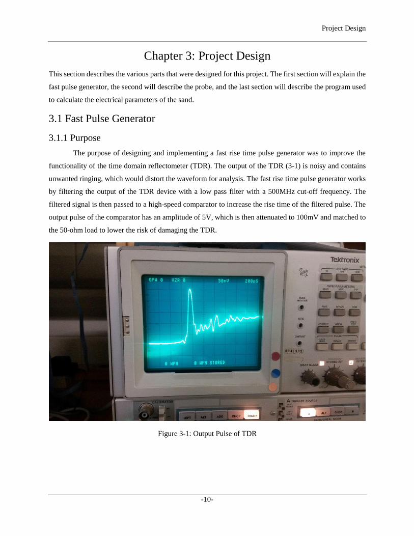
The purpose of designing and implementing a fast rise time pulse generator was to improve the

functionality of the time domain reflectometer (TDR). The output of the TDR (3-1) is noisy and contains

unwanted ringing, which would distort the waveform for analysis. The fast rise time pulse generator works

by filtering the output of the TDR device with a low pass filter with a 500MHz cut-off frequency. The

filtered signal is then passed to a high-speed comparator to increase the rise time of the filtered pulse. The

output pulse of the comparator has an amplitude of 5V, which is then attenuated to 100mV and matched to

the 50-ohm load to lower the risk of damaging the TDR.

Figure 3-1: Output Pulse of TDR

Project Design

-11-

3.1.2 Design and Simulations

A full design of the pulse generator is shown in figure 3-2. Details of how each section was designed

are in the next 3 sections.

Figure 3-2: Multisim Design of the Pulse Generator

3.1.2.1 Filter

The filter is designed to be a 5-pole pi Butterworth filter with a 500MHz cut-off. These values

selected as simulations demonstrated this specific configuration, which removed all the ringing and noise

from the TDR, while also keeping a faster rise time. The values of the filter were calculated using the two

equations below:

𝑔 = 2𝑠𝑖𝑛 (

2𝑘 − 1

2𝑛𝜋) 𝑘 = 1,2,3 …

3-1

Where n is the number of elements is the filter (5) and g is the prototype filter value.

𝐶 =

𝑔

𝑍 ∗ 𝑤 𝑎𝑛𝑑 𝐿 =

𝑍 ∗ 𝑔

𝑤

3-2

Where w is the cut off frequency (in rads/s) and Z is the characteristic impedance of the system

(50Ω).

The filter was simulated in LTSpice for the AC analysis and in Multisim for the transient analysis.

3.1.2.2 Comparator

The active component in the pulse generator is a transistor-transistor logic comparator from Texas

Instruments (TLV3501AIDBVR). This device runs off a single voltage supply (maximum 5V), has built in

hysteresis (6mV), has rail-to-rail input and output, and has a minimum rise time of 1.5nS. This comparator

was selected because it has the fastest rise time of purchasable comparators which has rail-to-rail output.

Project Design

-12-

Simulations on Multisim showed the device having a smooth 2ns rise time from 0 to ~5V (shown in figure

3-3).

Figure 3-3: Transient Analysis, Output of Comparator

3.1.2.3 Attenuator

The attenuator provides -20dB attenuation, this lowers the voltage output of the comparator to

~100mV. Its second purpose is to take the high impedance output of the comparator and match it to the

50Ω impedance of the system. Resistance values for the attenuator were calculated by an online

calculator.[2]

3.1.3 PCB Footprint and Manufacturing

The schematic for the PCB was finished in Multisim and the PCB footprint was designed on

Ultiboard 14, this is shown in figure 3-4. The PCB footprint was designed to limit stray inductance and the

signal path to be 50Ω. They were placed as close as possible together, and connections to the bottom ground

plane were connected by multiple vias, in order to limit stray inductance from filter components and

attenuator components. The 50Ω signal path width was calculated in Ultiboard; it was modeled as a micro-

strip transmission line.

Project Design

-13-

Figure 3-4: Footprint and 3D Rendering of the PCB

3.1.4 Results

The pulse generator was first tested with a low frequency function generator as the input and the

output was connected to a low frequency scope. This was to verify the generator would not damage the

expensive TDR. The result of this test is shown in figure 3-5. This test showed that the output has no DC

offset, its maximum output is attenuated to 250mV, and it has a ~5ns rise time (the bandwidth of this

oscilloscope limited the maximum visible rise time).

Figure 3-5: First Test of the Pulse Generator (Yellow: Pulse Generator Output, Blue: Low Frequency

Function Generator Output)

This successful test demonstrated that the pulse generator would not damage the expensive TDR,

which meant that the device could be tested on the TDR. The output of the pulse generator shown in figure

3-6 has a drastic improvement on the original TDR output (figure 3-2). The ringing is practically gone, and

there is no visible ringing at lower sampling speeds (5ns per division, which is used to capture the entire

Project Design

-14-

waveform). The final rise time of the pulse was found to be 2ns (which was found on the TDR device). One

potential problem with this rise time is that it is approaching the time it takes the wave to travel down the

probe. This can add potential problems in measuring conductivity (which is further discussed in chapter 6).

Figure 3-6: Output of the scope on the TDR

With successful tests of the pulse generator, the pulse generator was implemented within the testing

of the entire system.

3.2 Probe and Test Container

The TDR sends a pulse to the probe, which is suspended in the test container, containing the

medium such as sand. Due to the different electrical properties of the medium, the reflected wave will

influence the incident wave, changing the waveform seen by the TDR. By analyzing the waveform, the

permittivity and the conductivity of the medium can be calculated. The probe was designed to match the

characteristic impedance of the system (50Ω) while it is suspended in sand (the impedance changes to

~200Ω when the probe is suspended in air). The container was selected based on having the depth to contain

the full length of the probe, and the diameter to contain the electric field generated pulse traveling down

the probe.

Project Design

-15-

3.2.1 Probe design

Considering the feasibility of manufacturing and testing, an open-ended design was selected for the

probe. When the wave is transmitted to the end of the probe, it will be totally reflected unless the medium

used is overly conductive. The theory we use to calculate the conductivity is based on the totally reflected

wave at the end of the probe. This design will be more accurate with a lower salinity medium rather than

high salinity, since higher salinity mediums increases the conductivity of the medium which decreases the

reflection at the end of the probe. Considering the performance of the waveform and simplicity of

manufacturing and design, a three-rod probe design was selected. In comparison with a two-rod probe, the

three-rod probe has improved wave transmission since there is more energy surrounding the source rod. “In

comparison, the three-rod probe had a reduced sample area and more energy around the central rod.”

(Robinson p.458) [5]

The probe was constructed out of stainless steel because stainless steel is rigid and has a high

conductivity, it is inexpensive, and it can be machined by the machine shop at the University of Manitoba.

A rigid material is needed to avoid breaking of the probe, as well as to keep the probe’s structure when it

is inserted in a medium.

Figure 3-7: Left: Overview of Probe Design. Right: Detailed View of the Block

This design is shown in Figure 3-7. The sketch of the probe is shown in the left sketch in figure

3-7. The block and the rods are both stainless steel, and the surrounding part of the center rod is made by

polyethylene plastic (UHMW). The surrounding part of the center rod is the median of the block, which

Project Design

-16-

makes the characteristic impedance of the block to be same as the transmission line from the pulse

generator. This part works same as the coaxial cable, where the center rod works as the center core and the

steel block works as the metallic shield of the coaxial cable. From the characteristic impedance formula of

the coaxial cable:

𝑍𝑐 =

𝜂0

2𝜋√𝜀𝑟ln (

𝐷

𝑟)

3-3

Where 𝜂0 is the impedance of the free space, D is the diameter of the surrounding UHMW, r is the

inner rod diameter, and 𝜀𝑟 is relative permittivity of the UHMW, which is 2.3. To get the same characteristic

impedance as the transmission line, which is 50 Ω and, considering the size of the block, the diameter of

the of the surrounding UHMW (D) was selected to be 18mm and the diameter (r) to be 5mm.

The characteristic impedance of a transmission line is determined by the geometry and materials

used in to construct the transmission line. In the three-rod probe design, due to the different conditions of

the medium, the characteristic impedance can change drastically. There are three possible situations when

the transmitted wave reaches the beginning of the probe, which is inserted into the medium. If the

characteristic impedance of the probe is greater than that of the transmission line (which is 50 Ω), the wave

will reflect with same sign of the transmitted signal. If the impedance is less than the transmission line

impedance, the wave will reflect with the opposite sign of the transmitted signal. If the impedance is the

same as the transmission line, this will give no reflections at the start of the probe.

The characteristic impedance of the probe was selected to be between dry sand and de-ionized

water. De-ionized water was selected to minimize the maximum reflected values over the entire range.

Generally, the wet sand value of relative permittivity (which defines the characteristic impedance) is closer

to the dry sand value of 3 (opposed to the de-ionized water value of 80). The three-rod probe was designed

to have an impedance of 50 Ω at a permittivity of 16. The following equation found in [1] was used to

design the probe rod sizes and distance between each rod.

𝑍𝑐 =

𝜂0

4𝜋√𝜀𝑟ln (

1 − (𝐷𝑟 )

4

2 (𝐷𝑟 )

3 )

3-4

Where εr is the relative permittivity, D is the distance between rods, r is the radius of each rod, and

ηO is the characteristic impedance of free space. The radius of the rods was pre-selected to be 3mm as this

is a standard purchasable size for a stainless-steel rod. The distance between each rod was then calculated

to be 3.5cm to achieve the characteristic impedance at the relative permittivity that was defined.

Project Design

-17-

To connect the probe to the rest of system, a strong connection must be established. An SMA

connector (which is the type used by the transmission line) to Type-N flange is used to connect the

transmission line to the probe. Type-N flange gives a strong connection to the steel block. There is enough

contact area between the block and the flange to establish a very good connection to the ground. The center

rod (which carries the signal) is sufficiently isolated by the surrounding UHMW plastic from the block and

outer rods, and is connecting to the source of the Type-N flange. This design ensures mechanical stability

and has a good conduction with each individual part. The three-rod probe is manufactured by Cory Smit in

the machine shop of university of Manitoba. The outcome of the probe is shown in figure 3-8 below.

Figure 3-8: Finished Probe

Initially the probe was tested in the air, to test its functionality. The speed of the signal transmitting

in air is the speed of light (c = 3×108 m/s), the travel time of the pulse in air should be 2ns (which was

calculated using equation 2-2). In figure 3-9, the travel time of the pulse can be seen (the difference between

the second and third pulse) to be 2ns, this confirmed that the probe was working properly.

Project Design

-18-

Figure 3-9: Waveform with Probe in Air

3.2.3 Test Container

The main point of the project is to measure sand’s electrical parameters, which is its permittivity

and conductivity. The permittivity represents the water content of the soil, since water is the dominant effect

of the soil permittivity. The conductivity is affected by the content of different type of ions inside of the

soil. In this project, sand mixed with different amount of salt and de-ionized water is the type of soil that

will be tested. Sand was selected as the medium to be tested because it has predictable electrical properties.

The sand will be held in a test container, so testing can be done in the lab.

To ensure that most electrical fields will be contained in the container, a simulation of the probe

electrical fields was conducted in Matlab. The outcome of this simulation is shown in figure 3-10 and the

code can be found in Appendix A. The simulation is coded by implementing the Laplace Equation (∇2𝜑 =

0), the center rod was set to 1 V and side rods was set to 0 V in a 200×200 mm square. The contours show

the electric potential levels are from 1 V to 10-8 V. The yellow colours represent the higher electric potential

and the darker blue colours represent the lower electrical potential (where the outer contour is 10-8 V). The

diameter of the outer contour is about 13.5 cm. The amplitude of the real signal is around 0.1 V to 0.5 V

which is much smaller than the simulations 1 V, so the realized pattern is should be smaller than that in

figure 3-10. The container selected (a standard round 4-gallon bucket) has a diameter of 30 cm, which is

much greater than the 13.5 that specified in the simulation.

Project Design

-19-

Figure 3-10: Electrical Field Simulation of the Probe

3.3 TDR Signal Analysis Software

The designed software is based on Matlab graphical user interface (GUI). It will read the waveforms

from a text file by the corresponding file address. Time and voltage resolution of the TDR signal will also

need to be given by the user. After all parameters are submitted into the software by pressing the ‘Upload’

button, the input TDR signal waveform appears in the window. Then, pressing the ‘Analysis’ button, the

software will calculate permittivity, conductivity, and water content based on the TDR signal.

Project Design

-20-

3.3.1 Explanation of Graphical User Interface Window

Figure 3-11: Graphical User Interface (GUI) Window

1. Input box for entering the TXT file location

2. Input boxes for entering the Time Resolution, and Voltage Resolution

3. Upload button for uploading the file with parameters.

4. Edit boxes for showing the Permittivity, Conductivity, and Water Content.

5. Analysis button for evaluating the electrical parameter based on the input TDR signal.

3.3.2 Program Explanation

3.3.2.1 Function for getting the File address

Code:

function Filelocation_Callback(hObject, eventdata, handles) % hObject handle to Filelocation (see GCBO) % eventdata reserved - to be defined in a future version of MATLAB % handles structure with handles and user data (see GUIDATA) Filename =get(hObject,'string'); handles.Filename = char(Filename); guidata(gcbo,handles);

Explanation:

The function ‘get(h,'string')’ returns input object h in a string format. ‘Char( )’ converts the string

into character format. ‘Guidata( )’ function stores the file location as character format into the function

handles.

1

3

4

5

2

Project Design

-21-

3.3.2.2 Function for getting the Time/Voltage Resolution

Code:

function TimeRes_Callback(hObjectt, eventdata, handles) % hObject handle to TimeRes (see GCBO) % eventdata reserved - to be defined in a future version of MATLAB % handles structure with handles and user data (see GUIDATA) str_T =get(hObjectt,'string'); num_T = str2double(str_T); handles.numT = num_T; guidata(gcbo,handles);

function VoltRes_Callback(hObjecttt, eventdata, handles) % hObject handle to VoltRes (see GCBO) % eventdata reserved - to be defined in a future version of MATLAB % handles structure with handles and user data (see GUIDATA) str_V =get(hObjecttt,'string'); handles.numV = str2double(str_V); guidata(gcbo,handles);

Explanation:

The function ‘get(h,'string')’ returns input object h in string format. ‘Str2double( )’ then converts

the text string into double precision values. ‘Guidata( )’ function stores the time/voltage resolution as

numerical value into the function handle.

3.3.2.3 Function for uploading/plotting the waveform

I) Code:

FileID = fopen(handles.Filename); % to get the data tline = fgetl(FileID); C = strsplit(tline,','); handles.currentdata= str2double(C); % unedited waveform data (time step = 0.1ns)

Explanation:

A function ‘FileID = fopen(filename)’ opens the file that locate at ‘filename’, and returns an integer

file identifier. Then, the function ‘tline = fgetl(FileID)’ reads the file identifier, and returns the line from

the specified file. Because the output from ‘fgetl’ is in the format of ‘A, B, C, D…’, strsplit ( ) function

splits the character vector that contains comma-separated values, so the input character vector becomes the

character array [‘A’, ‘B’, ‘C’, ‘D’,…]. At the end of the function, the command ‘str2double’ converts the

character array into a numerical array, and store them into the function ‘handles’.

Project Design

-22-

II) Code:

handles.currentdata = handles.currentdata*handles.numV; distance = 0 - min(handles.currentdata); handles.currentdata = handles.currentdata + distance; dif = handles.currentdata(2:end) - handles.currentdata(1:end-1); % differentiation of the data dif = abs(dif); pek = findpeaks(dif); pek = sort(pek); % biggest peak should be initial pulse if pek(end) < 8; % checking to see if the initial pulse is there, shouldn’t be ever used handles.currentdata = handles.currentdata + 80; end handles.time = linspace(0,10*handles.numT,length(handles.currentdata)); % time array

plot(handles.time,handles.currentdata,'LineWidth',2,'color','g') grid on ylim([0,5*handles.numV]) guidata(hObject,handles);

Explanation:

The input waveform is represented by data points which are generated from time-based divisions

of the screen on the oscilloscope. This means the waveform needs to multiply by the voltage resolution.

Due to the DC offset from the oscilloscope, the waveform may not be positive, and this is not good for the

following analysis. To make sure the magnitude of plotted signal is always positive; the distance from

minimum value of TDR signal is defined as zero is and every other point will add this distance to ensure

the waveform is all positive.

There are two kinds of waveform for analysis. One includes the original pulse, and another does

not. The best way to distinguish these two kinds of waveform is detecting the increment between each point.

The original pulse contains the fastest changing amplitude, it is more difficult to distinguish the following

peaks, as shown in figures 3-12 and 3-13. Figure 3-12 does not contain the original pulse, and therefore it

is much easier to distinguish between the two reflections, the first being the moment the pulse reached the

start of the probe, and the second being the moment the pulse reaches the end of the probe, as described in

section 2. A problem arises when the impedance of the probe matches the line impedance and no reflection

occurs, which makes timing the pulse impossible. Figure 3-13, the two reflections are more difficult to

distinguish, but timing the reflection at the end of the probe will always be possible. The captured waveform

to be computed will always include the start of the pulse (figure 3-13), so the code can be standardized.

Project Design

-23-


Increase Omitted


Increase Included

Project Design

-24-

3.3.2.4 Function for analysing the signal waveform

I) Code:

df = handles.currentdata(2:end) - handles.currentdata(1:end-1);% find increment between points df = abs(df);% take absolute value of increment peks = findpeaks(df);% find all local maximums on the graph of absolute value of increment Mpeks = sort(peks); % sort, and find two largest local maximum Mpeks (Mpeks <1) = []; max1 = find(df == Mpeks (end));% find the location of the largest local maximum

Explanation:

For analysis of the signal, starting points and ending points during the signal rising parts need to be

located precisely. This is done by measuring the derivative of the signal. The output of the derivative is

shown in figure 3-14 and 3-15. The first part of the code calculates the derivative and then finds all the peak

points of the derivative (using ‘findpeaks’). The function then finds the location of the largest peak by first

sorting the peaks (‘Mpeks = sort(peks)’) in increment values from low to high. The function then removes

all peaks that have a value less than one (‘Mpeks (Mpeks <1) = []’). Finally, the function finds the largest

peak (‘find( )’).

II) Code:

a = 1; x = max1; % location of first peak while a <= (length(Mpeks)-1) % (a == 1)&&(c >= 1), used to find when the pulse hits the start and end

of the probe loc = find(d == Mpeks(end - a)); if length(loc) ~= 1 loc = loc(1); end if prod(abs(x-loc)>=25) x = [x loc]; end a = a + 1; end

Explanation:

After finding the first maximum, other large increment points (the next two reflection points) need

to be found as well. These points are found by finding the next maximum peaks later in the waveform. This

is done by not including the maximum peak and the surrounding 25 points (which corresponds to 2.5ns; 1

point = 0.1ns). When the next maximum is found, the surrounding 25 points will be excluded in the search,

so the other peaks can be found.

Project Design

-25-

III) Code:

mm = sort(x); % should contain the time of initial pulse, the end and/or start of probe if (length(mm)>=3)&&((mm(2)-mm(1))<200) % fix length of mm to 3 if start of probe mm = mm(1:3); end if ((mm(2)-mm(1))>=200) % fix mm to 2 if no start of probe mm = mm(1:2); end

Explanation:

After finding all maximum increment points, the points need to be sorted. There are two distinct

possible conditions. If the amount of maximum points is equal or greater than 3, and the amount of points

between the first two points are smaller than 200, this indicates that there are three rising parts. However,

if the amount of points between first two points are larger than 200, it means there are two rising parts. This

is because the resistance of sand is almost equal to the resistance of probe, so the amplitude of the reflected

signal from the starting point of the probe is around zero, and the signal received gets two rising parts. For

the former, three points are taken for analysis. In the case of the latter, two points are taken for analysis.

IV) Code:

i = 1; y = []; while i <= length(x) area = d(x(i)-20:x(i)+20); pkarea = findpeaks(area); pkarea1 = [pkarea>1]; d1 = pkarea1.*pkarea; d1(d1==0) = []; spoint = find(area == d1(1)); epoint = find(area == d1(end)); spoint = spoint(1); epoint = epoint(end); spoint = spoint + x(i) -21; epoint = epoint + x(i) -21; y = [y epoint spoint]; i = i+1; end

Explanation:

To reduce the negative influence of noise on the analysis, any points caused by noise must be

ignored. Shown in figure 3-14 are increments between each point, there are some noisy points near the peak

such as the point in figure 3-14 (2.153, 0.275). This point has a low magnitude of increment and would

Project Design

-26-

normally be used to check for the point at which the voltage begins to drop. However, the top part of figure

3-14 indicates that this is not accurate, and so points such as these will be labeled ‘cheat points’. To get the

real result, it is better to set a range (~2ns) from the maximum increment point to ignore any ‘cheat points’.

The first point that is out of this range and has low magnitude of increment will be considered as the ‘real

point’. The ‘real point’ in figure 3-14 is the point (4.012, 4.7).

Figure 3-14: Effect of Noise and Rising Time (2ns) on the Waveform (Top), and the Derivative (Simply

the Different Between Two Successive Points) of the Waveform (Bottom)

V) Code:

num1 = d(1:y(1)-1); num2 = d(y(2)+1:y(3) -1); num3 = d(y(4) +1:end); b1 = find(num1<0.4); % start of the initial pulse d1 = - b1(1) + y(1); b2 = find(num2<0.4); % end of initial pulse d2 = b2(1) + y(2);

Project Design

-27-

b3 = find(num2<0.4); % start of pulse at end of probe (V1 in cond calc) d3 = - b3(1) + y(3); b4 = find(num3<0.4); % end of pulse at end of probe d4 = b4(1)+ y(4); dd = [d1 d2 d3 d4]; % array of points

Explanation:

This code will find four ‘real points’, between which the signal waveform is divided into three

relevant parts. The first ‘real point’ is at the beginning of the pulse, the next is right after the initial pulse,

and the last two pulses are above and below the end pulse (when the wave hits the end of the probe). In

figure 3-15, it shows all four points that satisfy the condition. These points will be used to analysis the

conductivity of the medium.

Figure 3-15: Output of the TDR, the 4 Points Used to Find the Conductivity

VI) Code:

% Permittivity

d2 = (dd(2) + dd(1))*0.5;

d5 = (dd(3) + dd(4))*0.5;

time = (d5 - d2)*handles.time(2);

Prevpmt = (((3e8)*(time-13.425)*(10e-10))/0.6)^2; % first calculation of permittivity

d5 = (dd(3) + dd(4))*(0.5+0.0095*(Prevpmt/74)); % time correction

time = (d5 - d2)*handles.time(2);

pmt = (((3e8)*(time-13.425)*(10e-10))/0.6)^2; % actual permittivity

Project Design

-28-

handles.permittivity = pmt;

% Conductivity

de = max(handles.currentdata(d3:end-100));

d4 = find(handles.currentdata(d3:end-100)==de);

d4 = d4(1) + 15+ d3; % find V2 for conductivity calc

A = handles.currentdata(d3)*(2* handles.currentdata(d2) - handles.currentdata(d3));

B = handles.currentdata(d2)*(handles.currentdata(d4) - handles.currentdata(d3));

C = A/B;

D = log(C);

KK = (sqrt(pmt)/(120*pi*0.3))*D;

handles.Conductivity = KK;

% Water content

WC = (-530 + 292*pmt - 5.5*(pmt^2) + 0.043*(pmt^3))/(10^4);

if WC < 0

WC = 0;

end

handles.WaterContent = WC*100;

Explanation:

This section of the program finds the travelling time of the wave in the probe, which is used to find

the permittivity of the soil using equation (2.4). The program does this by finding the starting and ending

points of the rising edges (illustrated in figure 3-15), then calculating the midpoint of the edges and taking

the difference to calculate the time. This outputs the travel time from the TDR to the probe and back. Then,

to calculate the travel time down the probe, the travel time down the transmission line must be removed.

Since the properties of the transmission line should not change, this value is known from previous

experiments (13.425ns) and was hard-coded in.

This section of the program includes an ‘error compensation’ part. This part is included because

permittivity calculations can become less accurate as the travel time increases. Using the permittivity of de-

ionized water as the reference, it is possible to correct any error. Its theoretical value is 80, but experiments

with de-ionized water gave a permittivity output of 74. By analyzing the influence of error on time, it is

shown that there is a 0.95% error in the measured travel time for water. The formula:

𝐸𝑟𝑟𝑜𝑟 = 0.0095 ∗ (𝑝𝑒𝑟𝑣𝑝𝑚𝑡

74) 3-5

Where ‘pervpmt’ is the initial permittivity calculation. The resulting value will be used to

recalculate the midpoint of the second rising edge. Based on the new time measurement, the calculated

permittivity will be more accurate. From the permittivity and measured time, the water content and

conductivity can be calculated by the formulas (2.5) and (2.7).

Project Design

-29-

3.3.2.5 Function for analysing the signal waveform

I) Code:

handles.string2 = sprintf('%0.4f',handles.WaterContent);

handles.string1 = sprintf('%0.4f',handles.Conductivity);

handles.string = sprintf('%0.4f',handles.permittivity);

set(handles.edit5,'string',handles.string2);

set(handles.edit4,'string',handles.string1);

set(handles.edit3,'string',handles.string);

guidata(hObject,handles);

Explanation:

After getting all values about permittivity, conductivity, and water content, it shall display in the

output text box on the APP (figure 3-11). For better user experience, these values are showed in floating

point format.

Experiment Overview

-30-

Chapter 4: Experiment Overview

4.1 Multisim Experiment Design

Figure 4-1: Simulation of the Entire Experiment on the Multisim

Figure 4-1 is a screen capture of the simulation on Multisim. The original pulse from the TDR is

modeled as a Piecewise Linear Voltage Source (which is used to recreate the ringing of the pulse). The blue

parts in figure 4-1 are the pulse generator (explained in 3.1). R8, R9, and R10 are used to model a 3dB

attenuator, which is placed on the output of the TDR. The transmission line to the probe is modeled as a

lossless transmission line (W1), and the probe is modeled as a lossy transmission line (W2). To test different

mediums (such as de-ionized water, or dry sand) into which the probe will be inserted, the lossy

transmission line’s parameters (conductivity, resistivity, inductance and resistance) need to be changed as

illustrated in figure 4-2.

Experiment Overview

-31-

Figure 4-2: Parameters of Dry Sand of the Lossy Transmission Line for Simulating the Probe.

The resistance, inductance and capacitance are calculated by the following formulas:

Resistance: 𝑅 = 𝜌𝑙

𝐴

Inductance: 𝐿 = 2×10−7 ln (𝐺𝑀𝐷

𝐺𝑀𝑅)

Capacitance: 𝐶 = 2𝜋𝜖/ ln (𝐺𝑀𝐷

𝐺𝑀𝑅)

4-1

Where 𝜌 is the resistivity of the conductor material, which is 6.9 × 10-7 Ω·m for stainless steel, l is the

length of the probe, A is the cross-sectional area of the rod on the probe. GMD is Geometric Mean Distance,

the distance between each conductor (which is (𝐷 ∗ 𝐷 ∗ 2𝐷)^(1/3), where D is the distance between the

rods), and GMR is Geometric Mean Radius of the configuration. These equations were found in [9]. The

calculations to find the resistance, capacitance and inductance are performed in Matlab. Inductance

typically will not change since the magnetic properties of the medium will stay constant, and therefore it is

only based on the geometry of the probe. Resistance is based on material used to construct the probe.

Capacitance changes with a change in the permittivity of the medium. Permittivity and conductance are

both found by the experiment.

The calculated values are used to verify the waveform on the TDR and that the program is working

correctly. For example, in figure 4-3, the output waveform of dry sand (permittivity is ~3) was simulated.

The travel time of the pulse in the sand is around 3.3ns, and using this time in the equation in section 2.2.1

for permittivity gives a permittivity of 2.8 (a 6.7% error, which is acceptable for a simple simulation).

Experiment Overview

-32-

Figure 4-3: Dry Sand Simulation Output Waveform

4.2 Experiment Procedure

The experiment (measuring the electrical characteristics of sand at varying degrees of water

content) was conducted by adding a known volume of de-ionized water to the container which held the

sand. The waveform was captured by averaging 1000 samples (to remove noise) on the Tektronix

oscilloscope. The data was then transferred to a computer that can run Matlab for analysis of the waveform

with the program describe in section 3.3.2. This analysis outputted the permittivity, conductivity, and the

water content of the sand. These steps were reiterated until the sand is saturated with water. Once again,

these steps were reiterated, except the de-ionized water was replaced by a mixture of water and sodium

chloride salt, to change the conductivity of the medium.

The permittivity and conductivity values that were computed by the waveform data were used in

the Multisim experiment described in section 4.1. This was done to check if the waveforms from the TDR

matched the simulated waveforms, to verify the accuracy of the Matlab application (in section 3.3). For the

de-ionized water experiment, the calculations of the exact water content from equation 2-6 was used to

check the accuracy of the experiment. The results of the experiment are further discussed in the next chapter.

Experiment Results and Discussion

-33-

Chapter 5: Experiment Results and Discussion

5.1 Experimental results

5.1.1 De-ionized Water Experiment

This is the first experiment that was conducted; a known amount (1.1L) of de-ionized water was

added iteratively to the sand mixture. The results of this experiment are tabularized in table 3. Figure 5-1

compares 3 different waveforms that were collected in this experiment. Further discussion of this

experiment is done in section 5.2.1.

Test Number Permittivity Conductivity Water Content

1 (1.1L) 4.1 5.7e-3 5.86%

2 (2.2L) 6.8 8.0e-3 11.9%

3 (3.3L) 8.8 9.5e-3 16.3%

4 (4.4L) 11.0 9.6e-3 20.7%

5 (5.5L) 16.5 11.6e-3 31.2%

Table 3: Results from De-ionized Water Experiment

Figure 5-1: Comparing 3 Different Water Contents Waveforms


-34-

5.1.2 Sodium Chloride Salt Experiment

This experiment was completed after the sand was saturated with de-ionized water. The results of

this experiment are tabularized in table 4. Figure 5-2 compares 2 different amounts of salt that were added

to the saturated sand water mixture. Further discussion of this data is discussed in section 5.2.2.

Test Number Permittivity Conductivity Water Content

1 (tap water) 6.7 14.2e-3 11.9%

2 (6g Salt) 7.3 21.5e-3 13.3%

3 (13g Salt) 7.6 26.2e-3 13.9%

Table 4: Results from the Salt Water and Sand Experiment

Figure 5-2: Comparison 2 Differing Salt Amount Waveforms

5.2 Discussion of the Results

5.2.1 De-ionized Water Experiment

The first experiment was conducted with de-ionized water, and dry playground sand (results of

these can be found in Appendix B). Initially we measured the probe while it was in the air, submerged in

dry sand, and submerged in the de-ionized water. This was done to check the function of the probe and the

output of these tests can be found in Appendix B. The water content was calculated using equation (2.6).


-35-

The experiment began by adding 1.1L of water and mixing it into the sand until there was a

homogenous mixture of sand and water. The volume of the mixture was increased by about one liter from

the added water. This process continued until the sand was saturated with water. The final volume of added

water was 5.5L. As more water was added, the mixture began to decrease in volume as any air that was

trapped in the sand escaped. This effect can be seen in Table 5’s Test 5, the water content increased by

more than 10% due to most of the trapped air escaping from the mixture (the final volume of the mixture

was around 19L). The final mixture can be seen in figure 5-3.

Test Number Hand Calculated Water Content Application Calculated Water Content

1 5.50% 5.8%

2 10.4% 11.9%

3 14.8% 16.3%

4 18.8% 20.7%

5 28.9% 31.2%

Table 5: Comparison of the results

Figure 5-3: Saturated Sand-Water Mixture

The data in table 5 shows that as the water content of the mixture increased, the error calculated by

the TDR method increases; the maximum error difference being 2.2% (in the saturated sand water mixture).

This error could be contributed to the inaccurate measurements of the bottle used to measure the amount of

added water. This error is small enough to instil confidence that the project can measure accurately the

water content of sand.

Using the Multisim simulation described in chapter 4, the permittivity and conductivity was used

to find the transmission line characteristics, the output figures can be found in appendix B. The simulation


-36-

results for de-ionized water were relatively close, the simulated permittivity that was found showed a 5%

error, and the waveforms were close to matching as figure 5-4 and figure 5-5 shows.

Figure 5-4: TDR Waveform for Saturated Sand, Shown on the Matlab Application

Figure 5-5: Simulation Waveform for Saturated Sand

5.2.2 Sodium Chloride Salt Experiment

To test the accuracy of the TDR conductivity measurements, varying amounts of salt were tested

in a mixture of sand and water. At first 100g of salt was added, which unfortunately caused too much

attenuation and the pulse was completely absorbed into the sand mixture. New sand was then tested with

normal tap water, which was promising as the conductivity was found to be higher than the conductivity in

the de-ionized water experiment, which can be seen in table 4 in section 5.1.2. Lower amounts of salt (6g


-37-

and 7g) were then added, to further test different conductivities. After another 8g of salt were added, the

signal was not reflected and could not be measured.

To verify the conductivity measurements, the Multisim simulation was used, as manually

calculating a medium’s conductivity is much more difficult and requires unknown parameters of the

medium being used. The Multisim waveforms that were simulated did not appear to match the waveforms

that were collected by the TDR. It is not conclusive to say that the conductivity measurements in this

experiment are accurate, since there is no way to verify them. Most likely, the error lies in the simulation,

as simulations tend to output idealised results. Another possible source of the error in the conductivity

measurements will be explained in the next chapter.

Problems with the TDR

-38-

Chapter 6: Problems with the TDR

After testing, it was apparent that leaving the pulse generator on for more than 20 minutes degraded

the pulse output, illustrated in figure 6-1. Unfortunately, this was not seen until after testing was completed.

Fortunately, the testing of the de-ionized water was not affected since this test is based on the timing of the

pulse reaching the end of the probe.

Figure 6-1: Degradation of the TDR Pulse over Time

This may be the reason why the conductivity measurements did not output favorable values and

waveforms compared to the simulation. As the degradation drastically distorted the reflected wave, proper

voltage measurements to calculate the conductive would be much more difficult.

This degradation is believed to be from the TDR, as testing the pulse generator independently from

the TDR show no signs of degradation (even after running for 30 minutes). It is unknown why the pulse is

dropping. It may be caused by the TDR’s sampling head, noise leaking through the TDR’s pulse generator,

and/or a loading issue with the pulse generator.

Conclusion

-39-

Chapter 7: Conclusion

7.1 Conclusion

This project’s main purpose was to measure the electrical parameters of a given soil. Sand was

selected as the soil type to be tested, since it has predicable electrical properties. A simple 4-gallon bucket

was used to hold the sand since it was found to be large enough to contain all electrical fields that the probe

would be generating. The probe was designed to be optimized to test sand’s electrical properties. A 2ns rise

time pulse generator was designed to send a pulse to the probe and clean up the output of the TDR. Finally,

a program was developed to compute the electrical parameters of the waveform that was captured by the

TDR.

Several experiments were conducted to test different water contents of the sand. The experiment

with de-ionized water was successful, as the experimental data matched the simulated data and the hand

calculated data. The conductivity experiment with added salt was less conclusive as the simulated data did

not match the experimental data. Future experiments involving de-ionized water and salt, but without the

sand, could be done to verify if there were any problems in the previous conductivity experiments and to

conclusively say if the conductivity measurements are correct.

Future design of the pulse generator could include designing a sampling device to eliminate the

need of the old TDR. Improvements on the pulse generator could be done by amplifying the output so

mediums with higher conductivity can be measured. These improvements were outside of the project’s

current scope, and thus were not completed.

-40-

Appendix A – Further Code

A.1 Code for Probe Electrical Fields

A.1.1 C-Code for Implement Laplace Equation

//compile: gcc LaplaceEq.c -o Laplace

//run: ./Laplace

#include <stdio.h>

#include <math.h>

#define EPSILON 1e-8

#define X 201 //number of grid points in x directions

#define Y 201 //number of grid points in y directions

#define time_steps 5 //number of time steps

#define epsnaut 8.85e-12

#define epsr 10

#define center_x1 66



#define center_y 101

#define radius 3

int main(int argc, char *argv[])

int i,j,count,m,n;

int step;

double eps,enew,delta,absfy,X1,X2,Y1,Y2,q;

double time_max = 4; //max time in [sec]

double dt = time_max/time_steps; //time step

double t[X][Y];

double told[X][Y];

char fname[40];

FILE *out;

//initialize all grid values

for (i=0; i<X; i++)

for (j=0; j<Y; j++)

told[i][j] = 0.0;

t[i][j] = 0.0;

/* for all time steps */

for (step = 1; step <= time_steps; step++)

/* reset the boundary values each time step */

count=0;

do

count++;

eps = 0.0;

for (i=1; i<(X-1); i++)

for (j=1; j<(Y-1); j++)

for (m=98; m<=104; m++)

t[m][101]=1;

t[m-35][101]=0;

-41-

t[m+35][101]=0;

for (m=99; m<=103; m++)

t[m][100]=1;

t[m-35][100]=0;

t[m+35][100]=0;

t[m][102]=1;

t[m-35][102]=0;

t[m+35][102]=0;

for (m=100; m<=102; m++)

t[m][103]=1;

t[m-35][103]=0;

t[m+35][103]=0;

t[m][99]=1;

t[m-35][99]=0;

t[m+35][99]=0;

t[66][104]=0;

t[101][104]=1;

t[136][104]=0;

t[66][98]=0;

t[101][98]=1;

t[136][98]=0;

t[i][j]=(t[i+1][j]+t[i-1][j]+t[i][j+1]+t[i][j-1])*0.25;

for (i=1; i<(X-1); i++)

for (j=1; j<(Y-1); j++)

delta=fabs(t[i][j]-told[i][j]);

absfy=fabs(t[i][j]);

eps=delta/absfy;

for (i=1; i<(X-1); i++)

for (j=1; j<(Y-1); j++)

told[i][j] = t[i][j];

while(eps > EPSILON);

sprintf(fname,"time%03d.dat",step);

out = fopen(fname,"w");

for(j=0; j < Y; ++j)

for(i=0; i < X; ++i)

fprintf(out,"%e ",told[i][j]);

fprintf(out,"\n");

fclose(out);

printf("Time step: %d\r",step);

/* for all time steps */

printf("\n");

-42-

printf("pul:%e",q);

printf("\n");

return 0;

A.1.2 Matlab Code for Visualize the Contour

clc; close all; clear all;

phi=dlmread('time001.dat'); contour(1:201,1:201,phi,10); xlabel('x-axis'); ylabel('y-axis');

A.2 Matlab Code for Generating Plots

wf1 = dlmread('mix2_5ns.txt',','); wf2 = dlmread('mix1_5ns.txt',','); wf3 = dlmread('mix3_5ns.txt',','); wf4 = dlmread('mix4_5ns.txt',','); wf5 = dlmread('mix5_5ns.txt',','); wf6 = dlmread('mixsalt1.txt',','); wf7 = dlmread('mixsalt2.txt',','); wf8 = dlmread('unknownmix.txt',',');

waveforms = [wf1;wf2;wf3;wf4;wf5;wf6;wf7;wf8]; sample_t = 1e-10/1e-9; time = 0:sample_t:511*sample_t;

hold on Fs = 5/1e-10; N = length(wf1); Fnorm = 5e8/(Fs/2); df = designfilt('lowpassfir','FilterOrder',10,'CutoffFrequency',Fnorm); for i = 6:7 filteredwf(i,:) = filter(df,waveforms(i,:)); [startpeakval(i),startpeak(i)] = max(diff(filteredwf(i,:))); samestartwf(i,:) = [filteredwf(i,(startpeak(i)-10):end)

zeros(1,startpeak(i)-10-1)+filteredwf(i,end)]; normwf(i,:) = (samestartwf(i,:)-min(samestartwf(i,:))).*50; %in mv plot(time(1:300),normwf(i,1:300)); end title('TDR Waveforms with Differing Salt Contents') xlabel('Time (ns)') ylabel('Voltage (mV)') legend('5g of Salt added','13g of Salt added') hold off

-43-

Appendix B – Results

B.1 De-ionized Water Outputs

Sand with 1.1L of de-ionized water:

Figure 7-1: Sand with 1.1L of added De-ionized water

Figure 7-2: Simulation Result

The permittivity calculated from equation in section 2.2.1 is 4.2 (1.7% error).

-44-


Figure 7-3: Sand with 2.2L of added De-ionized water, TDR Waveform



-45-





-46-





-47-

B.2 Salt Water Outputs

Sand with Tap Water

Figure 7-9: Sand with Tap Water, TDR Waveform


-48-

The conductivity calculated from equation in section 2.2.1 is 0.0122 (14% error).

Sand with Tap Water and salt (6 grams)

Figure 7-11: Sand with Tap Water and salt (6 grams), TDR Waveform



-49-

Sand with Tap Water and salt (13 grams)

Figure 7-13: Sand with Tap Water and salt (13 grams), TDR Waveform



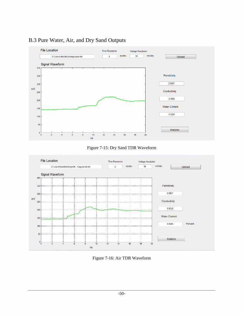
-50-

B.3 Pure Water, Air, and Dry Sand Outputs

Figure 7-15: Dry Sand TDR Waveform

Figure 7-16: Air TDR Waveform

-51-

Figure 7-17: Pure Water TDR Waveform

B.3 Pulse Generator Outputs

Figure 7-18: Pulse Generator Output with a Triangle Wave Input. Yellow is the Fast Pulse Generator and

Blue is the Input

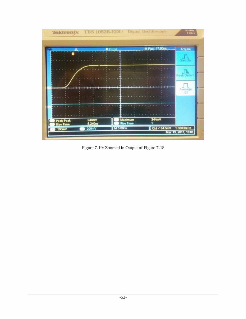
-52-

Figure 7-19: Zoomed in Output of Figure 7-18

-53-

Bibliography

[1]. Andrea Cataldo and Egidio De Benedetto et al, “Theoretical Background” in Broadband Reflectometry

for Enhanced Diagnostics and Monitoring Applications. Ed. Berlin, Germany: Springer-Verlag., 2011,

pp 38-39

[2]. Chemandy Electronics Ltd. (Feb 13 2016). Matching Pi Attenuator Calculator. Available:

http://chemandy.com/calculators/matching-pi-attenuator-calculator.htm

[3]. Henrik, H. N. (1995, June 11). Theoretical Background for the TDR Methodology. Proceedings of the

Symposium: Time Domain Reflectometry Applications in Soil Science held at the Research Centre

Foulum. Volume 3, pp: 9-23.

[4]. Konstantin, V. (2013, May 30). A low Cost Time Domain Reflectometry Circuit for printed Electronic

Applications. KTH Information and Communication Technology. Sweden: Stockholm.

[5]. Robinson, D. A., Jones, S. B., Wraith, J. M. ect. (2003). A Review of Advances in Dielectric and

Electrical Conductivity Measurement in Soils Using Time Domain Reflectometry. Vadose Zone

Journal. Vol 2. pp: 444–475.

[6]. Scott B. J., Jon, M. W., and Dani, O. (2002). Time domain reflectometry measurement principles and

applications. Hydrological processes hydrol. Process 16. Pp: 141-153.

[7]. Sochan, J., Vincent P. Drnevich, D., and Majdi, R. A. (2013, May). Temperature Corrections for Time

Domain Reflectometry Parameters. Journal of geotechnical and geoenvironmental engineering.

139(5), pp: 671-683.

[8]. Topp, G. C. (1980, June). Electromagnetic Determination of Soil Water Content: Measurements in

Coaxial Transmission Lines. Water resources research. Vol. 16, No. 3, pp: 574-582.

[9]. Taylor and Francis Group. (2006). Transmission Line Parameters. Available:

http://www.unioviedo.es/pcasielles/uploads/proyectantes/cosas_lineas.pdf

http://chemandy.com/calculators/matching-pi-attenuator-calculator.htm

http://www.unioviedo.es/pcasielles/uploads/proyectantes/cosas_lineas.pdf

g19 - time-domain reflectometer for soil electrical...

Documents