Chemometrics and Intelligent Laboratory Systems 107 (2011) 194–205

Contents lists available at ScienceDirect

Chemometrics and Intelligent Laboratory Systems

j ourna l homepage: www.e lsev ie r.com/ locate /chemolab

Further exploring rm2 metrics for validation of QSPR models

Probir Kumar Ojha 1, Indrani Mitra 1, Rudra Narayan Das 1, Kunal Roy ⁎Drug Theoretics and Cheminformatics Laboratory, Division of Medicinal and Pharmaceutical Chemistry, Department of Pharmaceutical Technology,Jadavpur University, Kolkata 700 032, India

Abbreviations: QSPR, quantitative structure–propertative structure–activity relationship; QSTR, quantitatiship; PRESS, predicted residuals sum of squares; SDEPpredictions; GFA, genetic function approximation; LOF,⁎ Corresponding author. Tel.: +91 98315 94140; fax:

E-mail address: kunalroy_in@yahoo.com (K. Roy).URL: http://sites.google.com/site/kunalroyindia/ (K.

1 These authors contributed equally to this work.

0169-7439/$ – see front matter © 2011 Elsevier B.V. Adoi:10.1016/j.chemolab.2011.03.011

a b s t r a c t

a r t i c l e i n f o

Article history:Received 18 January 2011Received in revised form 15 March 2011Accepted 20 March 2011Available online 12 April 2011

Keywords:QSPRQSARQSTRValidationrm2

Quantitative structure–property relationship (QSPR) models are widely used for prediction of properties,activities and/or toxicities of new chemicals. Validation strategies check the reliability of predictions of QSPRmodels. The classical metrics like Q2 and R2pred (Q2

ext) are commonly used, besides other techniques, forinternal validation (mostly leave-one-out) and external validation (test set validation) respectively. Recently,we have proposed a set of novel rm2 metrics which has been extensively used by us and other research groupsfor validation of QSPR models. In the present attempt, some additional variants of rm2 metrics have beenproposed and their applications in judging the quality of predictions of QSPR models have been shown byanalyzing results of the QSPR models obtained from three different data sets (n=119, 90, and 384). In eachcase, 50 combinations of training and test sets have been generated, and models have been developed basedon the training set compounds and subsequently applied for prediction of responses of the test setcompounds. Finally, models for a particular data set have been ranked according to the quality of predictions.The role of different validation metrics (including classical metrics and different variants of rm2 metrics) indifferentiating the “good” (predictive) models from the “bad” (low predictive) models has been studied.Finally, a set of guidelines has been proposed for checking the predictive quality of QSPR models.

ty relationship; QSAR, quanti-ve structure–toxicity relation-, standard deviation error oflack of fit.+91 33 2837 1078.

Roy).

ll rights reserved.

© 2011 Elsevier B.V. All rights reserved.

1. Introduction

Quantitative structure–property relationship (QSPR) modeling [1–4] represents applications of chemometric tools for exploringquantitative relationships between property (including biologicalactivity and toxicity) and descriptors quantifying informationencoded in the molecular structure. In a broad sense, QSPR includesquantitative structure–activity relationship (QSAR) and quantitativestructure–toxicity relationship (QSTR) studies. Apart from predictionof properties (properties/activities/toxicities) of novel molecules[5,6], QSPRs may be used for a mechanistic interpretation of the roleof physicochemical properties as determinants of biological activitiesor toxicities [7]. QSPRs have been widely used in drug design [8],pharmacokinetic modeling [9,10], agrochemistry [11] and predictivetoxicology [12,13]. Validation of QSPR models is an important aspectfor determination of reliability of such models [14–20]. There aredifferent approaches of validation including internal validation (usingthe same set of compounds used for model development) andexternal validation (using a different set of compounds not used for

model development) [21]. Defining an appropriate domain ofapplicability is also very important for the application of a QSPRmodel [22].

Internal validation is usually performed using leave-one-out (LOO)or leave-several-out (LSO) technique and the quality of predictions isexpressed in terms of the Q2 metric, which is calculated according tothe following equation:

Q2 = 1−∑ Ypred−Y

� �2

∑ Y−Y� �2 ð1Þ

In Eq. (1), Ypred and Y indicate predicted and observed activityvalues respectively and Y indicates mean activity value (of thetraining set). A model is considered acceptable when the value of Q2

exceeds 0.5. For external validation, usually, a test set is used and thequality of predictions is judged from the R2pred or Q2

ext metric, which iscalculated according to the following equation:

R2pred = 1−

∑ YpredðtestÞ−YðtestÞ� �2

∑ YðtestÞ−Ytraining

� �2 ð2Þ

In Eq. (2), Ypred(test) and Y(test) indicate predicted and observedactivity values respectively of the test set compounds and Y training

indicates mean activity value of the training set. For a predictive QSARmodel, the value of R2pred should be more than 0.5. In the expressions

195P.K. Ojha et al. / Chemometrics and Intelligent Laboratory Systems 107 (2011) 194–205

of Q2 and R2pred, differences between individual observed responses(training/test set) and Y of the training set are considered as thereference for comparing predicted residual values thus leading to anoverestimation of quality of predictions in cases of a data set withwide range of response values (Y-range). Different other variants ofthe Q2

ext metric have also been suggested [23]. Other importantmetrics in such classical validation schemes are predicted residualssum of squares (PRESS) and standard deviation error of predictions(SDEP) [21]. Apart from these, several other validation measures havebeen suggested in the literature: for example, Hou fitness function[24], Depczynski fitness functions [25], RQK fitness function [26–29],bootstrapping [30], model instability analysis [31], descriptive power[32,33], predictive power [33] and global modeling power [34] of amodel and Tropsha's criteria [35] for external validation. Hawkins etal. [36] proposed the concept of a “true” Q2 parameter, which can becalculated based on application of the variable selection strategy ateach validation cycle. Randomization [21] of the Y response is alsoperformed to check that the obtained model is not a result of chancefactors.

Recently, our group has proposed a novel metric rm2 [37] as an

additional validation parameter. This metric is calculated based on thecorrelations between the observed and predicted values with (r 2) andwithout (r02) intercept for the least squares regression lines as shownin the following equation:

r2m = r2 × 1−ffiffiffiffiffiffiffiffiffiffiffiffiffiffir2−r20

q� �ð3Þ

Themetric rm2 does not consider the differences between individualresponses and the training set mean and thus avoids overestimationof the quality of prediction due to a wide response range (Y-range)[38]. Initially, the rm

2 metric was used for the external validation usinga test set, but later it was used also for the training set validation(internal validation) using LOO-predicted values. It was shown [38]that rm

2(LOO) and rm

2(test) might serve as stricter metrics than Q2 and

R2pred respectively, especially for data sets with wide range of responsevalues, as the classical metrics compare the PRESS values with the sumof squared deviations of individual observed values from the trainingset mean. The metric rm

2 has also been used for validation using theentire set (combining training and test sets) using LOO-predictedvalues for the training set and model derived predicted values for thetest set. The rm

2(overall) value thus obtained may help in selecting the

best models from among comparable models showing differentpatterns in internal and external validation statistics [38]. The rm

2

metric has been used for validation of QSAR models in several studiesby our group [39–71] and also other research groups [72–124].

For the calculation of the rm2 metrics, we have so far arbitrarily usedthe observed response values in the y-axis and predicted values in thex-axis. However, the opposite may also be done. But this will result ina different value of the rm

2 metric (let us call it r /m2 ) unless the

predictions are perfect, i.e., when there is no intercept in the leastsquares regression line correlating observed and predicted values.This is because of the fact that the correlation between the observed(y) and predicted (x) values is same to that between the predicted (y)and observed (x) values in the presence of an intercept of thecorresponding least squares regression lines. However, this is not truewhen the intercept is set to zero. Thus, the value of r /m

2 will bedifferent from that of rm2 and the difference between these twometricsmay also be used as a measure of the goodness of predictions. Tofurther explore on these aspects, we have relooked and analyzed herethe results of the models reported in our previous work [38]. In thepresent study, we have tried to suggest a set of guidelines for checkingreliability of predictions of QSPR/QSAR/QSTRmodels. Themain idea ofthis paper is to suggest better measures of quality of predictionswhich may be used in addition to classical metrics during stringentvalidation of QSPR models. Attempt has also been made to indicate

how the classical metrics may overestimate the quality of predictionsin cases of data sets with wide response range due to consideration ofthe training set mean as the reference in their expressions. It may beemphasized that our objective in this work has not been exploring thebest models for different data sets; instead, we have tried to justifyapplication of some novel metrics in the validation of QSPR models.

2. Materials and methods

In the present study, results of the models reported in Ref. [38] forthree different data sets have been used for further analysis: (1) CCR5binding affinity data (IC50) of 119 piperidine derivatives [125–128];(2) ovicidal activity data (LC50) of 90 2-(2′,6′-difluorophenyl)-4-phenyl-1,3-oxazoline derivatives [129] and (3) Tetrahymena toxicity(IGC50) of 384 aromatic compounds [130]. The data sets are shown inTables S1–S3 in the Supplementary materials section. For the threedata sets (I, II and III), QSPR models were separately developed [38]from the genetic function approximation (GFA) technique [131] with5,000 crossovers using Cerius2 version 4.10 software [132]. Thedescriptors used were from the classes of topological, structural,physicochemical and spatial types (for details, the readers are referredto Ref. [38]). The whole descriptors matrices have been uploaded asexcel files in the Supplementary materials section. Based on clusteringusing the k-nearest neighbor method [133], each data set was dividedinto 50 combinations of training and test sets [38] so that both the testand training sets could represent all clusters and characteristics of thewhole dataset. Models were developed from a training set usinggenetic function approximation (GFA) [38] and a selected model(based on lack-of-fit ‘LOF’ score) was validated internally by the LOOmethod and then externally by predicting the response values of thecorresponding test set. Based on the results obtained from multiplemodels which were derived from different combinations of trainingand test sets, we tried to evaluate performance of different validationparameters [38]. We reported rm

2(LOO), rm2 (test) and rm

2(overall) values for

all 50 trials of each of the three data sets [38]. Different variants of therm2 metric reported in that paper [38] were based on the correlation

between observed (y-axis) and predicted (x-axis) values.In the present attempt, we have used the prediction data of 50

models for three data sets reported in Ref. [38]. In addition to usingthe reported Q2, R2

pred and rm2 values [38], we have calculated

additional validation metrics. Considering the predicted values inthe y-axis and observed values in the x-axis, we have now computedr/m2 metrics. For the brevity of discussions, we have limited our present

analysis to training sets and test sets (separately); analysis on thewhole sets (training and test sets combined) has been omitted here. Ineach case, we have also calculated the average of rm2 and correspond-ing r/m

2 values (r2m) and also the (absolute) difference between them(Δrm2). We have also noted the PRESS and SDEP values of each trial asthese values truly reflect the quality of predictions. The fraction (f1) ofthe total number of compounds (in a training/test set) havingpredicted residuals more than 1 log unit was also calculated as thisvalue may be an index of goodness of predictions for a model,arbitrarily considering that predictions are good when these arewithin one log unit from the corresponding observed values. Again,fraction (f2) of the number of compounds in a training/test set havingobserved response values more than 1.5 log units away from thetraining set mean was calculated. The higher is the value of thisfraction, the greater will be the value of the classical validationparameter (Q2 or R2pred) at a given level of quality of predictions (i.e.,PRESS). For each data set, among 50 trials, we have selected the best10 and worst 10 trials based on lowest and highest PRESS valuesrespectively. This was done separately for the training sets and testsets. Then we have calculated the average (mean) and standarddeviations of different rm2 metrics for the 10 best (and also 10 worst)trials. Similarly, we have also computed the average and standarddeviations for PRESS, SDEP, f1, f2 and Q2 (training set)/R2pred (test set)

196 P.K. Ojha et al. / Chemometrics and Intelligent Laboratory Systems 107 (2011) 194–205

for the 10 best (and 10 worst) trials. Then we have compared theaverage (mean) value of a particular metric for the 10 best trials withthe corresponding average for the 10 worst trials using t test forcomparison of means [134] to see whether the validation metrics canefficiently discriminate the good (predictive) models from the bad(low predictive) models. Finally, we have tried to explore anycommon pattern in the values of r2m and Δrm2 in good models so thata general recommendation can be made about these values whilechecking predictability of QSPRmodels. Note that our objective in thiswork has not been exploring the best models for each data set;instead, we have tried to justify application of the novel metrics r2m andΔrm2 in the validation of QSPR models.

Table 1Different validation metrics for the best 10 trials and worst 10 trials (for both training and

Training set

Models Trial no. PRESS SDEP f1 f2

Best 10trials

39 17.293 0.441 0.011 0.0229 21.268 0.489 0.045 0.04526 21.435 0.491 0.067 0.0451 22.527 0.503 0.056 0.03413 22.542 0.503 0.022 0.02233 23.395 0.513 0.067 0.07934 23.424 0.513 0.056 0.06746 23.523 0.514 0.045 0.05638 23.557 0.514 0.056 0.06724 23.787 0.517 0.034 0.045Mean (A)±s.e.

22.275±0.621

0.500±0.007

0.046±0.006

0.048±0.006

Worst 10trials

28 30.797 0.588 0.101 0.05623 30.818 0.588 0.067 0.04511 30.875 0.589 0.067 0.0456 30.965 0.590 0.090 0.0342 32.026 0.600 0.112 0.0673 32.111 0.601 0.101 0.04515 32.180 0.601 0.090 0.05629 32.276 0.602 0.101 0.06741 32.641 0.606 0.090 0.06742 34.047 0.619 0.112 0.067Mean (B)±s.e.

31.874±0.329

0.598±0.003

0.093±0.005

0.055±0.004

|A–B| 9.599 0.099 0.047 0.007t a(df=18) 13.653 12.481 6.076 0.936

Test set

Models Trial no. PRESS SDEP f1 f2

Best 10trials

42 7.519 0.501 0.033 0.03329 8.910 0.545 0.067 0.0333 9.502 0.563 0.067 0.10041 9.803 0.572 0.100 0.03318 11.040 0.607 0.133 0.13311 11.084 0.608 0.067 0.10015 11.694 0.624 0.100 0.0676 11.797 0.627 0.133 0.1334 11.929 0.631 0.067 0.06710 12.119 0.636 0.133 0.033Mean (C)±s.e.

10.540±0.486

0.591±0.014

0.090±0.011

0.073±0.013

Worst 10trials

48 18.929 0.794 0.133 0.00034 19.121 0.798 0.167 0.03327 19.234 0.801 0.233 0.03333 19.269 0.801 0.233 0.00012 19.304 0.802 0.200 0.00038 19.309 0.802 0.333 0.03343 20.885 0.834 0.300 0.0679 21.863 0.854 0.200 0.06726 22.407 0.864 0.233 0.06739 24.138 0.897 0.367 0.133Mean (D)±s.e.

20.446±0.569

0.825±0.011

0.240±0.023

0.043±0.013

|C–D| 9.906 0.234 0.150 0.030ta (df=18) 13.229 12.923 5.826 1.622

a t test for comparison of means A and B, or C and D (theoretical value of t at df 18=2.1

3. Results and discussion

The details of 50 combinations of training and test sets (includingindices selected in each trial, Sl. Nos. of test set compounds in eachtrial, cluster membership of the compounds and distance amongdifferent clusters, etc.) for three different data sets have been includedin Tables S4–S6 in the Supplementary materials section. The values ofdifferent validation metrics for the best 10 and the worst 10 trials(based on PRESS values) for both training and test sets separately forthree different data sets are shown in Tables 1–3. Note that, the set ofbest 10 trials for the training sets of a particular data set is not thesame as the set of worst 10 trials for the corresponding test sets. For a

test sets) of data set I.

Q2 rm2(LOO) r /m

2(LOO) r2m LOOð Þ Δrm2 (LOO) Y-range

0.701 0.517 0.702 0.610 0.185 3.1250.675 0.494 0.689 0.592 0.195 3.6020.645 0.467 0.676 0.572 0.209 3.5050.642 0.466 0.675 0.571 0.209 3.5050.640 0.463 0.674 0.569 0.211 3.5050.644 0.468 0.676 0.572 0.208 3.6020.629 0.454 0.668 0.561 0.214 3.6020.646 0.471 0.678 0.575 0.207 3.6020.628 0.454 0.669 0.562 0.215 3.5050.636 0.461 0.673 0.567 0.212 3.5050.649

±0.0070.472

±0.0060.678

±0.0030.575

±0.0050.207

±0.0030.558 0.369 0.628 0.499 0.259 3.5050.519 0.373 0.630 0.502 0.257 3.5050.519 0.372 0.629 0.501 0.257 3.5050.511 0.366 0.626 0.496 0.260 3.6020.569 0.378 0.631 0.505 0.253 3.6020.511 0.367 0.627 0.497 0.260 3.5050.502 0.360 0.624 0.492 0.264 3.5050.536 0.386 0.636 0.511 0.250 3.6020.510 0.367 0.627 0.497 0.260 3.6020.517 0.374 0.629 0.502 0.255 3.6020.525

±0.0070.371

±0.0020.629

±0.0010.500

±0.0020.258

±0.0010.123 0.100 0.049 0.075 0.051

12.343 15.229 14.558 15.012 15.823

R2pred rm2(test) r/m

2(test) r2m testð Þ Δrm2 (test) Y-range

0.595 0.578 0.323 0.451 0.255 2.8240.544 0.474 0.385 0.430 0.089 2.8240.595 0.566 0.229 0.398 0.337 3.3010.565 0.542 0.295 0.419 0.247 2.8240.542 0.529 0.183 0.356 0.346 3.2040.556 0.506 0.126 0.316 0.380 3.3010.523 0.500 0.241 0.371 0.259 3.3010.542 0.508 0.139 0.324 0.369 3.4770.438 0.391 0.230 0.311 0.161 3.4770.530 0.509 0.131 0.320 0.378 3.3010.543

±0.0140.510

±0.0170.228

±0.0280.369

±0.0160.282

±0.0310.167 0.179 0.009 0.094 0.170 2.6990.263 0.244 0.037 0.141 0.207 3.0790.212 0.219 0.051 0.135 0.168 3.0790.179 0.201 0.109 0.155 0.092 2.6990.117 0.133 −0.005 0.064 0.138 3.1760.253 0.266 0.078 0.172 0.188 3.1760.284 0.282 −0.068 0.107 0.350 3.1760.080 0.142 0.028 0.085 0.114 3.2040.233 0.179 0.007 0.093 0.172 3.1760.240 0.285 −0.030 0.128 0.315 3.1760.203

±0.0210.213

±0.0180.022

±0.0160.117

±0.0110.191

±0.0260.340 0.297 0.207 0.252 0.091

13.510 12.325 6.468 12.789 2.232

01 and p=0.05; two tailed test).

197P.K. Ojha et al. / Chemometrics and Intelligent Laboratory Systems 107 (2011) 194–205

particular data set, we have compared the average metrics of the best10 trials (for training or test sets) with the corresponding averagemetrics of the worst 10 trials using t test for comparison of means. Therange of response values in log units for each shown trial is alsomentioned in Tables 1–3. The values of different validation metrics(for both training and test sets) for all trials of the three different datasets are shown in Tables S7–S9 in the Supplementary materialssection.

3.1. Data set I

Table 1 shows the results for data set 1 (CCR5 binding affinitydata). First, we discuss the results for the training sets. The mean

Table 2Different validation metrics for the best 10 trials and worst 10 trials (for both training and

Training set

Models Trial no. PRESS SDEP f1 f2

Best 10trials

44 55.104 0.900 0.191 0.47135 60.619 0.944 0.324 0.45645 66.245 0.987 0.250 0.44127 66.313 0.988 0.279 0.45619 67.249 0.994 0.309 0.45626 68.279 1.002 0.279 0.47118 72.325 1.031 0.309 0.45648 73.563 1.040 0.324 0.42624 73.991 1.043 0.309 0.47122 74.326 1.045 0.279 0.456Mean (A)±s.e.

67.802±1.979

0.998±0.015

0.285±0.013

0.456±0.004

Worst 10trials

15 93.100 1.170 0.324 0.48506 93.366 1.172 0.338 0.45634 93.895 1.175 0.338 0.44132 93.939 1.175 0.426 0.44110 98.025 1.201 0.412 0.45609 98.140 1.201 0.324 0.47142 98.149 1.201 0.353 0.45637 102.991 1.231 0.412 0.44108 103.545 1.234 0.338 0.47102 104.053 1.237 0.368 0.485Mean (B)±s.e.

97.920±1.379

1.200±0.008

0.363±0.012

0.460±0.005

|A–B| 30.118 0.202 0.078 0.004t a(df=18) 12.487 11.832 4.368 0.635

Test set

Models Trial no. PRESS SDEP f1 f2

Best 10trials

08 22.192 1.004 0.409 0.45509 24.558 1.057 0.455 0.45506 26.170 1.091 0.364 0.54546 26.361 1.095 0.273 0.63634 26.662 1.101 0.273 0.54515 27.039 1.109 0.409 0.40917 27.516 1.118 0.364 0.50037 27.616 1.120 0.500 0.54542 27.859 1.125 0.409 0.50013 29.388 1.156 0.409 0.500Mean (C)±s.e.

26.536±0.626

1.098±0.013

0.386±0.023

0.509±0.020

Worst 10trials

30 52.236 1.541 0.409 0.45549 52.722 1.548 0.500 0.45516 52.856 1.550 0.409 0.45540 55.273 1.585 0.500 0.40921 59.899 1.650 0.409 0.40945 60.460 1.658 0.591 0.54541 61.544 1.673 0.409 0.45544 62.948 1.692 0.636 0.45535 67.093 1.746 0.500 0.50048 70.823 1.794 0.455 0.591Mean (D)±s.e.

59.586±2.010

1.644±0.028

0.482±0.026

0.473±0.018

|C–D| 33.050 0.546 0.096 0.036ta (df=18) 15.698 17.858 2.792 1.342

a t test for comparison of means A and B, or C and D (theoretical value of t at df 18=2.1

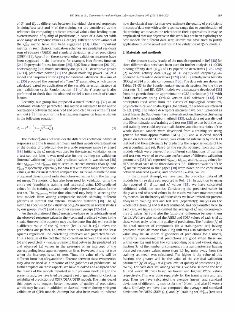
PRESS for the best 10 trials (training set) is 22.275 while that for theworst 10 trials is 31.874. The difference between the mean PRESSvalues is significant at pb0.05 as shown by the corresponding t valueat the degree of freedom (df) of 18. Similarly, the absolute differencebetweenmean SDEP values for the sets of best 10 andworst 10 trials is0.099 with a t value of 12.481 at the df of 18. This confirms that thetwo sets of 10 trials are statistically significantly different based on thequality of predictions (i.e., PRESS and SDEP values). Now, we haveexamined how the other validation metrics have differentiated thesetwo sets. ThemeanQ2 value of the best 10 trials (0.649) is significantlydifferent from that of the worst 10 trials (0.525) as evident from a tvalue of 12.243 at the df of 18. The ranges of the response values for all20 trials are not very wide (lower than 4 log units) and the mean

test sets) of data set II.

Q2 rm2(LOO) r /m

2(LOO) r2m LOOð Þ Δrm2 (LOO) Y-range

0.723 0.551 0.720 0.636 0.169 6.1000.704 0.536 0.712 0.624 0.176 6.1000.663 0.496 0.689 0.593 0.193 6.1000.672 0.503 0.692 0.598 0.189 6.1000.665 0.499 0.691 0.595 0.192 6.0900.666 0.504 0.696 0.600 0.192 6.1000.656 0.493 0.687 0.590 0.194 6.1000.623 0.466 0.674 0.570 0.208 6.1000.637 0.475 0.677 0.576 0.202 6.0900.612 0.457 0.669 0.563 0.212 5.1900.662

±0.0110.498

±0.0090.691

±0.0050.594

±0.0070.193

±0.0040.523 0.390 0.636 0.513 0.246 5.1900.548 0.408 0.644 0.526 0.236 6.1000.517 0.387 0.634 0.510 0.247 6.1000.540 0.407 0.644 0.526 0.237 6.1000.513 0.381 0.630 0.505 0.249 6.1000.521 0.391 0.636 0.513 0.245 6.1000.485 0.365 0.624 0.494 0.259 5.1800.486 0.368 0.624 0.496 0.256 6.0900.468 0.357 0.620 0.489 0.263 5.1900.510 0.384 0.631 0.508 0.247 6.1000.511

±0.0080.384

±0.0050.632

±0.0030.508

±0.0040.249

±0.0030.151 0.114 0.059 0.086 0.056

11.347 10.763 10.345 10.627 11.132

R2pred rm

2(test) r/m

2(test) r2m testð Þ Δrm2 (test) Y-range

0.714 0.684 0.440 0.562 0.244 6.0900.633 0.535 0.128 0.331 0.407 5.1800.600 0.585 0.270 0.427 0.315 5.1600.636 0.550 0.372 0.461 0.178 5.1700.656 0.635 0.371 0.503 0.264 5.1800.652 0.573 0.239 0.406 0.334 6.0800.597 0.597 0.300 0.448 0.297 5.1700.614 0.559 0.219 0.389 0.340 5.1900.656 0.634 0.360 0.497 0.274 6.1000.613 0.577 0.257 0.417 0.320 6.0800.637

±0.0110.593

±0.0140.296

±0.0290.444

±0.0210.297

±0.0200.213 0.260 0.057 0.158 0.203 5.1800.151 0.173 0.071 0.122 0.102 5.1400.203 0.243 0.089 0.166 0.154 5.1800.125 0.149 0.028 0.088 0.121 5.150

−0.028 0.129 0.168 0.148 0.039 5.1500.200 0.173 0.018 0.095 0.155 5.1600.077 0.140 0.077 0.108 0.063 5.1800.136 0.169 0.029 0.099 0.140 5.170

−0.002 0.108 0.073 0.091 0.035 5.1600.077 0.134 0.049 0.092 0.085 5.1700.115

±0.0270.168

±0.0150.066

±0.0140.117

±0.0100.110

±0.0170.522 0.425 0.230 0.327 0.187

18.152 20.066 7.161 14.355 7.145

01 and p=0.05; two tailed test).

Table 3Different validation metrics for the best 10 trials and worst 10 trials (for both training and test sets) of data set III.

Training set

Models Trial no. PRESS SDEP f1 f2 Q2 rm2(LOO) r /m

2(LOO) r2m LOOð Þ Δrm2 (LOO) Y-range

Best 10trials

25 30.180 0.324 0.010 0.024 0.772 0.715 0.791 0.753 0.076 3.4131 32.685 0.337 0.007 0.028 0.766 0.716 0.790 0.753 0.074 3.4050 33.826 0.343 0.007 0.045 0.774 0.726 0.796 0.761 0.070 3.8515 33.876 0.343 0.004 0.028 0.769 0.724 0.795 0.760 0.071 3.8917 33.968 0.343 0.007 0.028 0.755 0.706 0.784 0.745 0.078 3.799 33.996 0.344 0.010 0.031 0.759 0.712 0.787 0.750 0.075 3.8930 34.338 0.345 0.007 0.038 0.771 0.720 0.793 0.757 0.073 3.7949 35.951 0.353 0.004 0.031 0.764 0.719 0.791 0.755 0.072 3.951 36.356 0.355 0.014 0.035 0.758 0.711 0.787 0.749 0.076 3.8923 36.597 0.356 0.017 0.035 0.755 0.710 0.785 0.748 0.075 3.89Mean (A)±s.e.

34.177±0.599

0.344±0.003

0.009±0.001

0.032±0.002

0.764±0.002

0.716±0.002

0.790±0.001

0.753±0.002

0.074±0.001

Worst 10trials

22 46.652 0.402 0.028 0.035 0.693 0.679 0.761 0.720 0.082 3.9528 46.663 0.403 0.024 0.045 0.696 0.696 0.770 0.733 0.074 3.9544 47.051 0.404 0.017 0.038 0.699 0.684 0.764 0.724 0.080 3.9545 47.208 0.405 0.010 0.038 0.677 0.676 0.757 0.717 0.081 3.8529 47.591 0.407 0.017 0.045 0.690 0.681 0.761 0.721 0.080 3.9541 47.628 0.407 0.010 0.038 0.692 0.684 0.763 0.724 0.079 3.9512 48.323 0.410 0.010 0.038 0.672 0.669 0.752 0.711 0.083 3.855 49.108 0.413 0.031 0.038 0.671 0.659 0.747 0.703 0.088 3.7919 49.912 0.416 0.024 0.035 0.676 0.673 0.754 0.714 0.081 3.953 52.253 0.426 0.017 0.042 0.660 0.668 0.750 0.709 0.082 3.85Mean (B)±s.e.

48.239±0.557

0.409±0.002

0.019±0.002

0.039±0.001

0.683±0.004

0.677±0.003

0.758±0.002

0.717±0.003

0.081±0.001

|A–B| 14.061 0.065 0.010 0.007 0.082 0.039 0.032 0.036 0.007t a(df=18) 17.190 16.877 17.346 10.138 12.3 11.042 5.154 3.77 3.070

Test set

Models Trial no. PRESS SDEP f1 f2 R2pred rm

2(test) r/m

2(test) r2m testð Þ Δrm2 (test) Y-range

Best 10trials

3 12.601 0.362 0.0104 0.031 0.750 0.721 0.654 0.688 0.067 3.5129 12.895 0.367 0.0104 0.010 0.746 0.727 0.590 0.659 0.137 3.0140 12.924 0.367 0.0208 0.031 0.758 0.722 0.585 0.654 0.137 3.4327 13.427 0.374 0.0104 0.031 0.744 0.742 0.605 0.674 0.137 3.4128 13.436 0.374 0.0104 0.031 0.736 0.686 0.646 0.666 0.040 3.3126 13.579 0.376 0.0104 0.052 0.781 0.752 0.621 0.687 0.131 3.8945 13.799 0.379 0.0000 0.042 0.834 0.753 0.630 0.692 0.123 3.6522 14.169 0.384 0.0208 0.042 0.731 0.688 0.544 0.616 0.144 3.7348 14.236 0.385 0.0104 0.031 0.737 0.714 0.576 0.645 0.138 3.5516 14.333 0.386 0.0313 0.052 0.753 0.728 0.597 0.663 0.131 3.95Mean (C)±s.e.

13.540±0.191

0.375±0.003

0.014±0.003

0.035±0.004

0.757±0.010

0.723±0.007

0.605±0.011

0.664±0.007

0.119±0.011

Worst 10trials

11 24.326 0.503 0.021 0.063 0.583 0.590 0.430 0.510 0.160 3.651 24.397 0.504 0.021 0.031 0.551 0.559 0.379 0.469 0.180 3.5542 25.814 0.519 0.042 0.042 0.522 0.473 0.418 0.446 0.055 3.3015 26.303 0.523 0.052 0.073 0.545 0.518 0.392 0.455 0.126 3.8517 26.599 0.526 0.052 0.052 0.595 0.594 0.430 0.512 0.164 3.959 27.123 0.532 0.042 0.052 0.572 0.577 0.394 0.486 0.183 3.8531 27.178 0.532 0.031 0.063 0.580 0.559 0.463 0.511 0.096 3.9523 27.633 0.537 0.042 0.031 0.497 0.478 0.376 0.427 0.102 3.7037 29.371 0.553 0.063 0.031 0.382 0.385 0.288 0.337 0.097 3.0425 30.628 0.565 0.0729 0.073 0.575 0.594 0.430 0.512 0.164 3.95Mean (D)±s.e.

26.937±0.625

0.529±0.006

0.044±0.005

0.051±0.005

0.540±0.020

0.533±0.022

0.400±0.015

0.466±0.017

0.133±0.014

|C–D| 13.397 0.154 0.030 0.016 0.217 0.191 0.205 0.198 0.014ta (df=18) 20.498 23.112 5.048 2.395 9.763 8.292 11.059 10.463 0.800

a t test for comparison of means A and B, or C and D (theoretical value of t at df 18=2.101 and p=0.05; two tailed test).

198 P.K. Ojha et al. / Chemometrics and Intelligent Laboratory Systems 107 (2011) 194–205

fractions ( f2) of the compounds having response values more than 1.5log units away from the training set mean are quite low for both thesets (around 5%). Thus, the values of the Q2 metric for these trials donot appear to be over-optimistic [38]. Again, the mean rm

2(LOO) value

for the best 10 trials is highly penalized (0.472) while that for theworst 10 trials is still lower (0.371). Though the metric rm

2(LOO)

differentiates the two classes efficiently (t value being 15.229 at the dfof 18), the metric appears to underestimate the quality of predictions.Interchanging the axes (vide supra), r/m2 (LOO) values were calculatedand mean values of this metric for both 10 best and 10 worst trialswere higher than the corresponding mean Q2 values. The average ofrm2(LOO) and r/m

2(LOO) values appears as a compromise between

overestimation and underestimation of the quality of predictions.

The mean r2m LOOð Þ for the best 10 trials (0.575) is significantly differentfrom that of the worst 10 trials (0.500) as evidenced from the t test.The difference between rm

2(LOO) and r/m

2(LOO) values (Δrm2) was also

calculated. The mean Δrm2 (LOO) for the best 10 trials is just above 0.2while the value of mean Δrm2 (LOO) for the worst 10 trials is 0.258 andthese values are significantly different at pb0.05.

Now we will discuss the results for the test sets. Like training sets,here also, the sets of best 10 trials and worst 10 trials are statisticallysignificantly different in terms of the quality of predictions asevidenced by the t test for comparison of means showing t values of13.229 and 12.923 for PRESS and SDEP respectively. However, it mustbe noted here that the best 10 trials based on PRESS values for the testsets are not same as those based on PRESS values for the training sets.

199P.K. Ojha et al. / Chemometrics and Intelligent Laboratory Systems 107 (2011) 194–205

It is awesome to note that six out of 10 best trials for the training set(trial nos. 39, 9, 26, 33, 34, 38) are actually members of the set of 10worst trials for the test sets (Table 4). Again, seven out of 10 worsttrials (trial nos. 11, 6, 3, 15, 29, 41, 42) for the training sets are actuallymembers of the set of 10 best trials for the test sets (Table 4). Thiscorroborates that internal validation has no relation with externalvalidation as we observed in reference [37]. For all the shown trials,the ranges of response values are not very wide (less than 4 log units),and thus the metric R2pred does not appear to show overoptimisticpicture about quality of predictions [38]. The difference betweenmean R2

pred values for the sets of best 10 and worst 10 trials is 0.340which is significant at pb0.05. The values of mean r /m

2(test) for the two

sets are close to the corresponding mean R2pred values. However, the

r /m2(test) metric, calculated after interchange of axes (vide supra),

showed highly penalized values. The average of rm2 (test) and r/m2(test)

values (i.e., r2m for the test sets) is a compromise between over-estimation and underestimation of quality of predictions, and it canefficiently differentiate the two sets of best and worst trials (asevident from the t value significant at pb0.05). The differencebetween rm

2(test) and r /m

2(test) values (Δrm2 for the test sets) was also

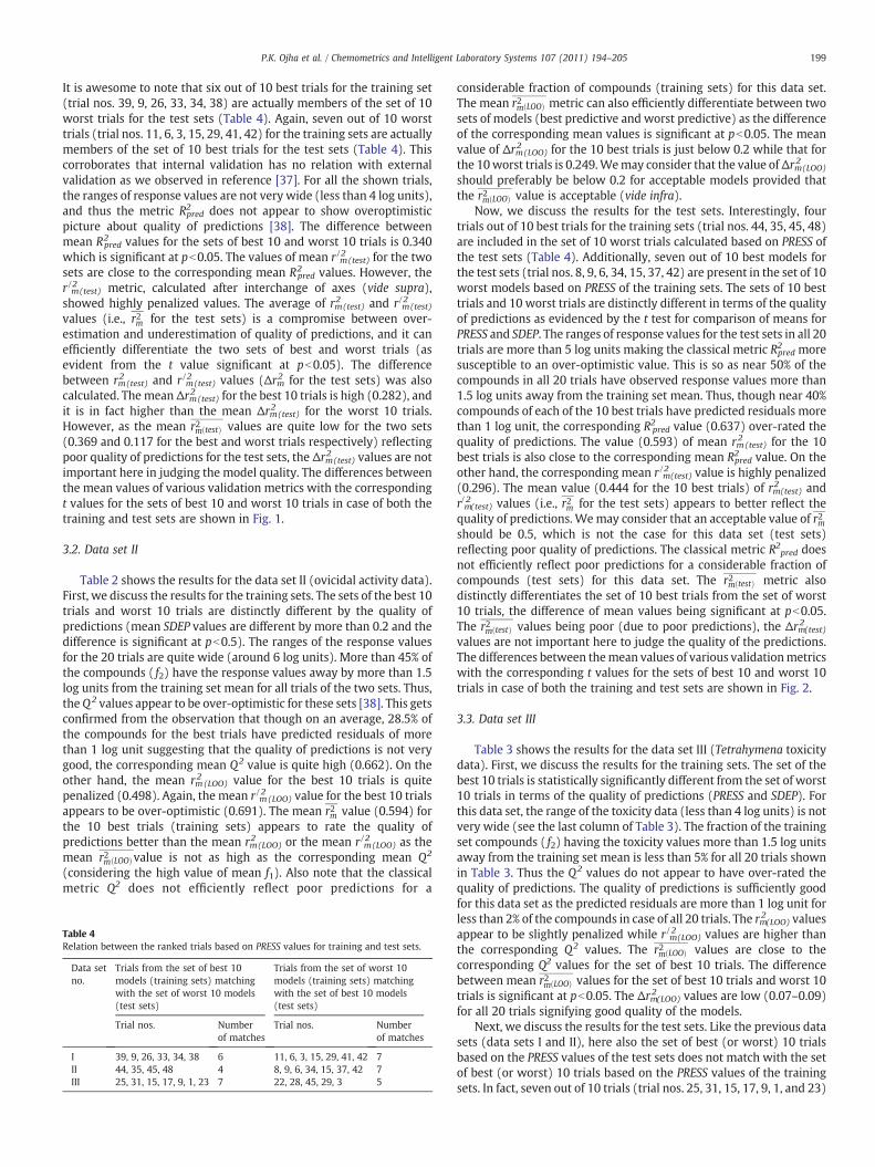
calculated. ThemeanΔrm2 (test) for the best 10 trials is high (0.282), andit is in fact higher than the mean Δrm2 (test) for the worst 10 trials.However, as the mean r2m testð Þ values are quite low for the two sets(0.369 and 0.117 for the best and worst trials respectively) reflectingpoor quality of predictions for the test sets, the Δrm2 (test) values are notimportant here in judging the model quality. The differences betweenthe mean values of various validation metrics with the correspondingt values for the sets of best 10 and worst 10 trials in case of both thetraining and test sets are shown in Fig. 1.

3.2. Data set II

Table 2 shows the results for the data set II (ovicidal activity data).First, we discuss the results for the training sets. The sets of the best 10trials and worst 10 trials are distinctly different by the quality ofpredictions (mean SDEP values are different by more than 0.2 and thedifference is significant at pb0.5). The ranges of the response valuesfor the 20 trials are quite wide (around 6 log units). More than 45% ofthe compounds ( f2) have the response values away by more than 1.5log units from the training set mean for all trials of the two sets. Thus,the Q2 values appear to be over-optimistic for these sets [38]. This getsconfirmed from the observation that though on an average, 28.5% ofthe compounds for the best trials have predicted residuals of morethan 1 log unit suggesting that the quality of predictions is not verygood, the corresponding mean Q2 value is quite high (0.662). On theother hand, the mean rm

2(LOO) value for the best 10 trials is quite

penalized (0.498). Again, the mean r /m2(LOO) value for the best 10 trials

appears to be over-optimistic (0.691). The mean r2m value (0.594) forthe 10 best trials (training sets) appears to rate the quality ofpredictions better than the mean rm

2(LOO) or the mean r /m

2(LOO) as the

mean r2m LOOð Þvalue is not as high as the corresponding mean Q2

(considering the high value of mean f1). Also note that the classicalmetric Q2 does not efficiently reflect poor predictions for a

Table 4Relation between the ranked trials based on PRESS values for training and test sets.

Data setno.

Trials from the set of best 10models (training sets) matchingwith the set of worst 10 models(test sets)

Trials from the set of worst 10models (training sets) matchingwith the set of best 10 models(test sets)

Trial nos. Numberof matches

Trial nos. Numberof matches

I 39, 9, 26, 33, 34, 38 6 11, 6, 3, 15, 29, 41, 42 7II 44, 35, 45, 48 4 8, 9, 6, 34, 15, 37, 42 7III 25, 31, 15, 17, 9, 1, 23 7 22, 28, 45, 29, 3 5

considerable fraction of compounds (training sets) for this data set.The mean r2m LOOð Þ metric can also efficiently differentiate between twosets of models (best predictive and worst predictive) as the differenceof the corresponding mean values is significant at pb0.05. The meanvalue of Δrm2 (LOO) for the 10 best trials is just below 0.2 while that forthe 10worst trials is 0.249.Wemay consider that the value ofΔrm2 (LOO)should preferably be below 0.2 for acceptable models provided thatthe r2m LOOð Þ value is acceptable (vide infra).

Now, we discuss the results for the test sets. Interestingly, fourtrials out of 10 best trials for the training sets (trial nos. 44, 35, 45, 48)are included in the set of 10 worst trials calculated based on PRESS ofthe test sets (Table 4). Additionally, seven out of 10 best models forthe test sets (trial nos. 8, 9, 6, 34, 15, 37, 42) are present in the set of 10worst models based on PRESS of the training sets. The sets of 10 besttrials and 10 worst trials are distinctly different in terms of the qualityof predictions as evidenced by the t test for comparison of means forPRESS and SDEP. The ranges of response values for the test sets in all 20trials are more than 5 log units making the classical metric R2pred moresusceptible to an over-optimistic value. This is so as near 50% of thecompounds in all 20 trials have observed response values more than1.5 log units away from the training set mean. Thus, though near 40%compounds of each of the 10 best trials have predicted residuals morethan 1 log unit, the corresponding R2pred value (0.637) over-rated thequality of predictions. The value (0.593) of mean rm

2(test) for the 10

best trials is also close to the corresponding mean R2pred value. On theother hand, the corresponding mean r /m

2(test) value is highly penalized

(0.296). The mean value (0.444 for the 10 best trials) of rm2 (test) andr/m

2(test) values (i.e., r2m for the test sets) appears to better reflect the

quality of predictions. Wemay consider that an acceptable value of r2mshould be 0.5, which is not the case for this data set (test sets)reflecting poor quality of predictions. The classical metric R2pred doesnot efficiently reflect poor predictions for a considerable fraction ofcompounds (test sets) for this data set. The r2m testð Þ metric alsodistinctly differentiates the set of 10 best trials from the set of worst10 trials, the difference of mean values being significant at pb0.05.The r2m testð Þ values being poor (due to poor predictions), the Δrm2(test)values are not important here to judge the quality of the predictions.The differences between themean values of various validationmetricswith the corresponding t values for the sets of best 10 and worst 10trials in case of both the training and test sets are shown in Fig. 2.

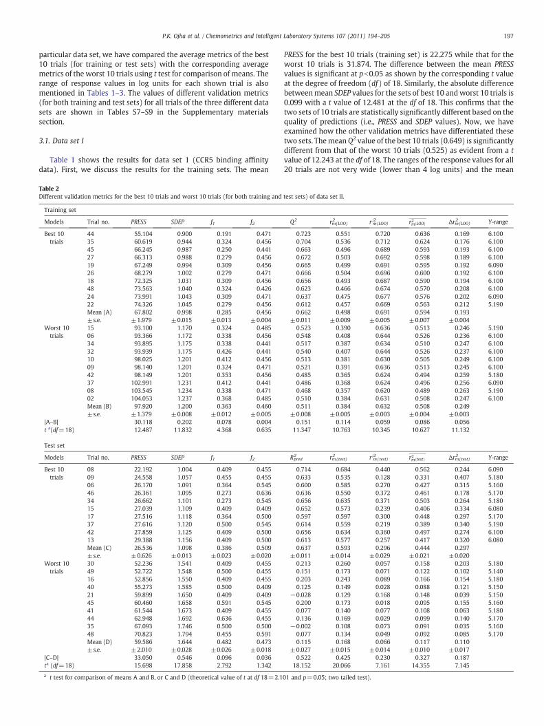
3.3. Data set III

Table 3 shows the results for the data set III (Tetrahymena toxicitydata). First, we discuss the results for the training sets. The set of thebest 10 trials is statistically significantly different from the set of worst10 trials in terms of the quality of predictions (PRESS and SDEP). Forthis data set, the range of the toxicity data (less than 4 log units) is notvery wide (see the last column of Table 3). The fraction of the trainingset compounds ( f2) having the toxicity values more than 1.5 log unitsaway from the training set mean is less than 5% for all 20 trials shownin Table 3. Thus the Q2 values do not appear to have over-rated thequality of predictions. The quality of predictions is sufficiently goodfor this data set as the predicted residuals are more than 1 log unit forless than 2% of the compounds in case of all 20 trials. The rm2(LOO) valuesappear to be slightly penalized while r /m

2(LOO) values are higher than

the corresponding Q2 values. The r2m LOOð Þ values are close to thecorresponding Q2 values for the set of best 10 trials. The differencebetween mean r2m LOOð Þ values for the set of best 10 trials and worst 10trials is significant at pb0.05. The Δrm2(LOO) values are low (0.07–0.09)for all 20 trials signifying good quality of the models.

Next, we discuss the results for the test sets. Like the previous datasets (data sets I and II), here also the set of best (or worst) 10 trialsbased on the PRESS values of the test sets does not match with the setof best (or worst) 10 trials based on the PRESS values of the trainingsets. In fact, seven out of 10 trials (trial nos. 25, 31, 15, 17, 9, 1, and 23)

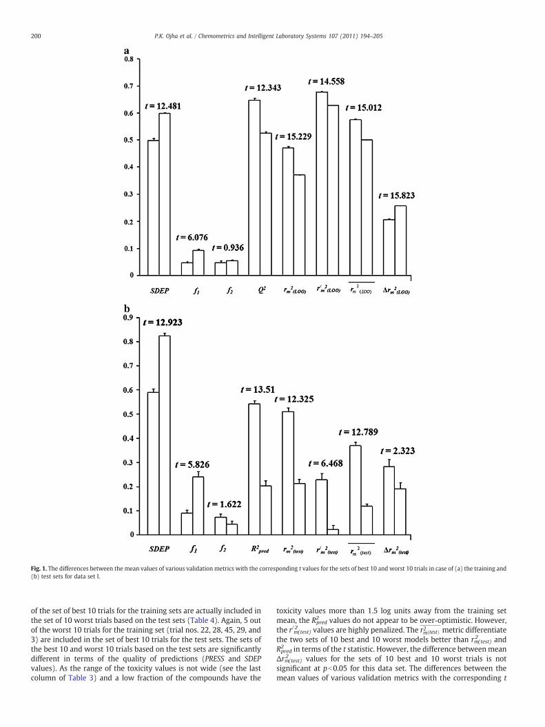
Fig. 1. The differences between the mean values of various validation metrics with the corresponding t values for the sets of best 10 and worst 10 trials in case of (a) the training and(b) test sets for data set I.

200 P.K. Ojha et al. / Chemometrics and Intelligent Laboratory Systems 107 (2011) 194–205

of the set of best 10 trials for the training sets are actually included inthe set of 10 worst trials based on the test sets (Table 4). Again, 5 outof the worst 10 trials for the training set (trial nos. 22, 28, 45, 29, and3) are included in the set of best 10 trials for the test sets. The sets ofthe best 10 and worst 10 trials based on the test sets are significantlydifferent in terms of the quality of predictions (PRESS and SDEPvalues). As the range of the toxicity values is not wide (see the lastcolumn of Table 3) and a low fraction of the compounds have the

toxicity values more than 1.5 log units away from the training setmean, the R2pred values do not appear to be over-optimistic. However,the r/m

2(test) values are highly penalized. The r2m testð Þ metric differentiate

the two sets of 10 best and 10 worst models better than rm2(test) and

R2pred in terms of the t statistic. However, the difference betweenmeanΔrm2(test) values for the sets of 10 best and 10 worst trials is notsignificant at pb0.05 for this data set. The differences between themean values of various validation metrics with the corresponding t

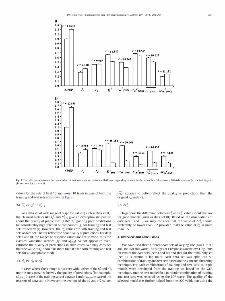
Fig. 2. The differences between the mean values of various validation metrics with the corresponding t values for the sets of best 10 and worst 10 trials in case of (a) the training and(b) test sets for data set II.

201P.K. Ojha et al. / Chemometrics and Intelligent Laboratory Systems 107 (2011) 194–205

values for the sets of best 10 and worst 10 trials in case of both thetraining and test sets are shown in Fig. 3.

3.4. r2m vs. Q2 or R2pred

For a data set of wide range of response values (such as data set II),the classical metrics like Q2 and R2pred give an overoptimistic pictureabout the quality of predictions (Table 2) ignoring poor predictionsfor considerably high fraction of compounds ( f1 for training and testsets respectively). However, the r2m values for both training and testsets of data set II better reflect the poor quality of predictions. For datasets I and III, the ranges of response values are not so wide, thus theclassical validation metrics (Q2 and R2pred) do not appear to over-estimate the quality of predictions in such cases. We may considerthat the value of r2m should be more than 0.5 for both training and testsets for an acceptable model.

3.5. r2m vs. rm2 or r/m

2

In cases where the Y-range is not very wide, either of the rm2 and r /m2

metrics may penalize heavily the quality of predictions (for example,rm2(LOO) in case of the training sets of data set I and r /m

2(test) in case of the

test sets of data set I). However, the average of the rm2 and r /m

2 values

(r2m) appears to better reflect the quality of predictions than theoriginal rm2 metrics.

3.6. Δrm2

In general, the difference between rm2 and r /m

2 values should be lowfor good models (such as data set III). Based on the observations ofdata sets I and II, we may consider that the value of Δrm2 shouldpreferably be lower than 0.2 provided that the value of r2m is morethan 0.5.

4. Overview and conclusions

We have used three different data sets of varying size (n=119, 90and 384) for this work. The ranges of Y responses are below 4 log unitsfor two of the data sets (sets I and III) and that for the remaining set(set II) is around 6 log units. Each data set was split into 50combinations of training and test sets based on the k-means clusteringtechnique. For each combination of training and test sets, multiplemodels were developed from the training set based on the GFAtechnique, and the best model for a particular combination of trainingand test sets was selected using the LOF score. The quality of theselected model was further judged from the LOO validation using the

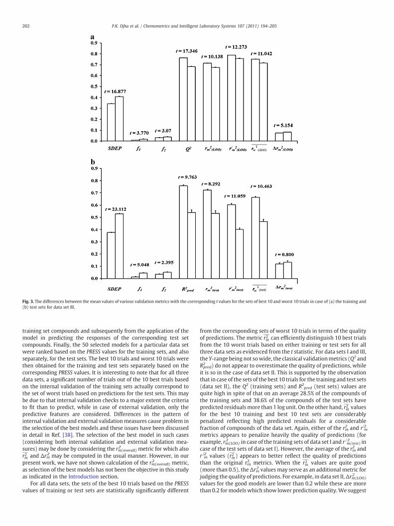
Fig. 3. The differences between the mean values of various validation metrics with the corresponding t values for the sets of best 10 and worst 10 trials in case of (a) the training and(b) test sets for data set III.

202 P.K. Ojha et al. / Chemometrics and Intelligent Laboratory Systems 107 (2011) 194–205

training set compounds and subsequently from the application of themodel in predicting the responses of the corresponding test setcompounds. Finally, the 50 selected models for a particular data setwere ranked based on the PRESS values for the training sets, and alsoseparately, for the test sets. The best 10 trials and worst 10 trials werethen obtained for the training and test sets separately based on thecorresponding PRESS values. It is interesting to note that for all threedata sets, a significant number of trials out of the 10 best trials basedon the internal validation of the training sets actually correspond tothe set of worst trials based on predictions for the test sets. This maybe due to that internal validation checks to a major extent the criteriato fit than to predict, while in case of external validation, only thepredictive features are considered. Differences in the pattern ofinternal validation and external validationmeasures cause problem inthe selection of the best models and these issues have been discussedin detail in Ref. [38]. The selection of the best model in such cases(considering both internal validation and external validation mea-sures) may be done by considering the rm

2(overall) metric for which also

r2m and Δrm2 may be computed in the usual manner. However, in ourpresent work, we have not shown calculation of the rm

2(overall) metric,

as selection of the best models has not been the objective in this studyas indicated in the Introduction section.

For all data sets, the sets of the best 10 trials based on the PRESSvalues of training or test sets are statistically significantly different

from the corresponding sets of worst 10 trials in terms of the qualityof predictions. The metric r2m can efficiently distinguish 10 best trialsfrom the 10 worst trials based on either training or test sets for allthree data sets as evidenced from the t statistic. For data sets I and III,the Y-range being not sowide, the classical validationmetrics (Q2 andR2pred) do not appear to overestimate the quality of predictions, whileit is so in the case of data set II. This is supported by the observationthat in case of the sets of the best 10 trials for the training and test sets(data set II), the Q2 (training sets) and R2pred (test sets) values arequite high in spite of that on an average 28.5% of the compounds ofthe training sets and 38.6% of the compounds of the test sets havepredicted residualsmore than 1 log unit. On the other hand, r2m valuesfor the best 10 training and best 10 test sets are considerablypenalized reflecting high predicted residuals for a considerablefraction of compounds of the data set. Again, either of the rm

2 and r/m2

metrics appears to penalize heavily the quality of predictions (forexample, rm2 (LOO) in case of the training sets of data set I and r /m

2(test) in

case of the test sets of data set I). However, the average of the rm2 and

r /m2 values (r2m) appears to better reflect the quality of predictions

than the original rm2 metrics. When the r2m values are quite good(more than 0.5), the Δrm2 values may serve as an additional metric forjudging the quality of predictions. For example, in data set II,Δrm2 (LOO)values for the good models are lower than 0.2 while these are morethan 0.2 for models which show lower prediction quality.We suggest

203P.K. Ojha et al. / Chemometrics and Intelligent Laboratory Systems 107 (2011) 194–205

the following guidelines for judging predictive quality of QSPRmodels:

1. In addition to the classical validation parameters (Q2 and R2pred),different rm2 values should additionally be checked for both trainingand test sets (vide points 2 and 3 below).

2. The values of both r2m LOOð Þ for the training set and r2m testð Þ for the testset should be more than 0.5.

3. If the point 2 above is satisfied, then Δrm2 values should be checkedfor both training and test sets. The values of Δrm2 (LOO) and Δrm2(test)should preferably be lower than 0.2.

Supplementarymaterials related to this article can be found onlineat doi:10.1016/j.chemolab.2011.03.011.

Acknowledgments

The authors thank the University Grants Commission, New Delhi,Indian Council of Medical Research, NewDelhi andMinistry of HumanResource and Development, Govt. of India for providing financialassistance to PKO, IM and RND.

Appendix A

NotationsQ2 Classical internal validation parameter (see Eq. (1))R2pred Classical external validation parameter (see Eq. (2))r 2 Determination coefficient for the least squares regression

line (with intercept) correlating observed (y-axis) andpredicted (x-axis) values

r02 Determination coefficient for the least squares regression

line (without intercept) correlating observed (y-axis) andpredicted (x-axis) values

rm2 Novel validationmetric calculated according to Eq. (3) using

observed (y-axis) and predicted (x-axis) valuesr /m

2 Novel validationmetric calculated according to Eq. (3) usingobserved (x-axis) and predicted (y-axis) values

r2m Average of rm2 and r /m2

Δrm2 Absolute difference between rm2 and r /m

2

f1 The fraction of the total number of compounds (in atraining/test set) having predicted residuals more than 1 logunit

f2 The fraction of the number of compounds in a training/testset having observed response values more than 1.5 log unitsaway from the training set mean

References

[1] P. Buchwald, N. Bodor, Computer-aided drug design: the role of quantitativestructure–property, structure–activity and structure–metabolism relationships(QSPR, QSAR, QSMR), Drugs Future 27 (2002) 577–588.

[2] H.-J. Huang, H.W. Yu, C.-Y. Chen, C.-H. Hsu, H.-Y. Chen, K.-J. Lee, F.-J. Tsai, C.Y.C.Chen, Current developments of computer-aided drug design, J. Taiwan Inst.Chem. Eng. 41 (2010) 623–635.

[3] D.G. Sprous, R.K. Palmer, J.T. Swanson, M. Lawless, QSAR in the pharmaceuticalresearch setting: QSAR models for broad, large problems, Curr. Top. Med. Chem.10 (2010) 619–637.

[4] C. Nantasenamat, C. Isarankura-Na-Ayudhya, T. Naenna, V. Prachayasittikul, Apractical overview of quantitative structure–activity relationship, EXCLI J.8 (2009) 74–88.

[5] J. Hu, X. Zhang, Z.Wang, A review on progress in QSPR studies for surfactants, Int.J. Mol. Sci. 11 (2010) 1020–1047.

[6] P.R. Duchowicz, E.A. Castro, QSPR studies on aqueous solubilities of drug-likecompounds, Int. J. Mol. Sci. 10 (2009) 2558–2577.

[7] J. Verma, V.M. Khedkar, E.C. Coutinho, 3D-QSAR in drug design — a review, Curr.Top. Med. Chem. 10 (2010) 95–115.

[8] C.A. Lipinski, Overview of hit to lead: the medicinal chemist's role from HTSretest to lead optimization hand off, Topics Med. Chem. 5 (2010) 1–24.

[9] D.E. Mager, Quantitative structure–pharmacokinetic/pharmacodynamic rela-tionships, Adv. Drug Deliv. Rev. 58 (2006) 1326–1356.

[10] L.G. Valerio Jr., Computational science in drugmetabolism and toxicology, ExpertOpin. Drug Metab. Toxicol. 6 (2010) 781–784.

[11] B. Bordás, T. Komíves, A. Lopata, Ligand-based computer-aided pesticide design.A review of applications of the CoMFA and CoMSIA methodologies, Pest Manag.Sci. 59 (2003) 393–400.

[12] N. Fjodorova, M. Novich, M. Vrachko, V. Smirnov, N. Kharchevnikova, Z.Zholdakova, S. Novikov, N. Skvortsova, D. Filimonov, V. Poroikov, E. Benfenati,Directions in QSAR modeling for regulatory uses in OECD member countries, EUand in Russia, J. Environ. Sci. Health C Environ. Carcinog. Ecotoxicol. Rev. 26(2008) 201–236.

[13] S. Kar, K. Roy, Predictive toxicology using QSAR: a perspective, J. Indian Chem.Soc. 87 (2010) 1455–1515.

[14] A. Tropsha, Best practices for QSAR model development, validation, andexploitation, Mol. Inf. 29 (2010) 476–488.

[15] T. Scior, J.L. Medina-Franco, Q.-T. Do, K. Martínez-Mayorga, J.A. Yunes Rojas, P.Bernard, How to recognize and workaround pitfalls in QSAR studies: a criticalreview, Curr. Med. Chem. 16 (2009) 4297–4313.

[16] J.C. Dearden, M.T.D. Cronin, K.L.E. Kaiser, How not to develop a quantitativestructure–activity or structure–property relationship (QSAR/QSPR), SAR QSAREnviron. Res. 20 (2009) 241–266.

[17] K. Roy, On some aspects of validation of predictive quantitative structure–activity relationship models, Expert Opin. Drug Discov. 2 (2007) 1567–1577.

[18] L. Eriksson, J. Jaworska, A.P. Worth, M.T. Cronin, R.M. McDowell, P. Gramatica,Methods for reliability and uncertainty assessment and for applicabilityevaluations of classification- and regression-based QSARs, Environ. HealthPerspect. 111 (2003) 1361–1375.

[19] K. Roy, J.T. Leonard, On selection of training and test sets for the development ofpredictive QSAR models, QSAR Comb. Sci. 25 (2006) 235–251.

[20] P.P. Roy, J.T. Leonard, K. Roy, Exploring the impact of the size of training sets forthe development of predictive QSAR models, Chemom. Intell. Lab. Syst. 90(2008) 31–42.

[21] S. Wold, L. Eriksson, Statistical validation of QSAR results, in: H. van deWaterbeemd (Ed.), Chemometric Methods inMolecular Design,Weinheim, VCH,1995, pp. 309–318.

[22] P. Gramatica, Principles of QSAR models validation: internal and external, QSARComb. Sci. 26 (2007) 694–701.

[23] V. Consonni, D. Ballabio, R. Todeschini, Comments on the definition of the Q2

parameter for QSAR validation, J. Chem. Inf. Model. 49 (2009) 1669–1678.[24] T.-J. Hou, J. Wang, X. Xu, Applications of genetic algorithms on the structure–

activity correlation study of a group of non-nucleoside HIV-1 inhibitors,Chemom. Intell. Lab. Syst. 45 (1999) 303–310.

[25] U. Depczynski, V.J. Frost, K. Molt, Genetic algorithms applied to the selection offactors in principal component regression, Anal. Chim. Acta 420 (2000) 217–227.

[26] R. Todeschini, V. Consonni, A. Mauri, M. Pavan, Detecting "bad" regressionmodels: multicriteria fitness functions in regression analysis, Anal. Chim. Acta515 (2004) 199–208.

[27] R. Todeschini, Data correlation, number of significant principal components andshape of molecules. The K correlation index, Anal. Chim. Acta 348 (1997)419–430.

[28] R. Todeschini, V. Consonni, A. Maiocchi, The K correlation index: theorydevelopment and its applications in chemometrics, Chemom. Intell. Lab. Syst.46 (1999) 13–29.

[29] A.J. Miller, Subset Selection in Regression, Chapman & Hall, London, UK, 1990.[30] R. Wehrens, H. Putter, L.M.C. Buydens, The bootstrap: a tutorial, Chemom. Intell.

Lab. Syst. 54 (2000) 35–52.[31] E. Kolossov, R. Stanforth, The quality of QSAR models: problems and solutions,

SAR QSAR Environ. Res. 18 (2007) 89–100.[32] S. Sagrado, M.T.D. Cronin, Application of the modeling power approach to

variable subset selection for GA-PLS QSAR models, Anal. Chim. Acta 609 (2008)169–174.

[33] H. Martens, M. Martens, Multivariate Analysis of Quality. An Introduction, JohnWiley & Sons Ltd, Chichester, 2001.

[34] S. Sagrado, M.T.D. Cronin, Diagnostic tools to determine the quality of“transparent” regression-based QSARs: the “modeling power” plot, J. Chem.Inf. Model. 46 (2006) 1523–1532.

[35] A. Golbraikh, A. Tropsha, Beware of q2! J. Mol. Graph. Model. 20 (2002) 269–276.[36] D.M. Hawkins, S.C. Basak, D. Mills, Assessing model fit, by cross-validation,

J. Chem. Inf. Comput. Sci. 43 (2003) 579–586.[37] P.P. Roy, K. Roy, On some aspects of variable selection for partial least squares

regression models, QSAR Comb. Sci. 27 (2008) 302–313.[38] P.P. Roy, S. Paul, I. Mitra, K. Roy, On two novel parameters for validation of

predictive QSAR models, Molecules 14 (2009) 1660–1701.[39] P.P. Roy, K. Roy, Comparative QSAR studies of CYP1A2 inhibitor flavonoids using

2D and 3D descriptors, Chem. Biol. Drug Des. 72 (2008) 370–382.[40] S. Paul, K. Roy, Exploring 2D and 3D QSARs of 2,4-diphenyl-1,3-oxazolines for

ovicidal activity against Tetranychus urticae, QSAR Comb. Sci. 28 (2009) 406–425.[41] K. Roy, S. Paul, Docking and 3D QSAR studies of protoporphyrinogen oxidase

inhibitor 3H-pyrazolo[3,4-d][1,2,3]triazin-4-one derivatives, J. Mol. Model. 16(2010) 137–153.

[42] I. Mitra, A. Saha, K. Roy, Quantitative structure–activity relationship modeling ofantioxidant activities of hydroxybenzalacetones using quantum chemical, physi-cochemical and spatial descriptors, Chem. Biol. Drug Des. 73 (2009) 526–536.

[43] I. Mitra, K. Roy, A. Saha, QSAR of antilipid peroxidative activity of substitutedbenzodioxoles using chemometric tools, J. Comput. Chem. 30 (2009) 2712–2722.

204 P.K. Ojha et al. / Chemometrics and Intelligent Laboratory Systems 107 (2011) 194–205

[44] K. Roy, G. Ghosh, QSTR with extended topochemical atom indices 10. Modelingof toxicity of organic chemicals to humans using different chemometric tools,Chem. Biol. Drug Des. 72 (2008) 383–394.

[45] K. Roy, P.P. Roy, Comparative chemometric modeling of cytochrome 3A4inhibitory activity of structurally diverse compounds using stepwise MLR, FA-MLR, PLS, GFA, G/PLS and ANN techniques, Eur. J. Med. Chem. 44 (2009)2913–2922.

[46] K. Roy, P.P. Roy, Exploring QSAR and QAAR for inhibitors of cytochrome P4502A6 and 2A5 enzymes using GFA and G/PLS techniques, Eur. J. Med. Chem. 44(2009) 1941–1951.

[47] K. Roy, I. Mitra, A. Saha, Molecular shape analysis of antioxidant and squalenesynthase inhibitory activities of aromatic tetrahydro-1,4-oxazine derivatives,Chem. Biol. Drug Des. 74 (2009) 507–516.

[48] K. Roy, P.L.A. Popelier, Exploring predictive QSAR models for hepatocyte toxicityof phenols using QTMS descriptors, Bioorg. Med. Chem. Lett. 18 (2008)2604–2609.

[49] K. Roy, P.L.A. Popelier, Exploring predictive QSAR models using quantumtopological molecular similarity (QTMS) descriptors for toxicity of nitroaro-matics to Saccharomyces cerevisiae, QSAR Comb. Sci. 27 (2008) 1006–1012.

[50] K. Roy, P.L.A. Popelier, Predictive QSPR modeling of acidic dissociation constant(pKa) of phenols in different solvents, J. Phys. Org. Chem. 22 (2009) 186–196.

[51] I. Mitra, P.P. Roy, S. Kar, P. Ojha, K. Roy, On further application of rm2 as ametric forvalidation of QSAR models, J. Chemometrics 24 (2010) 22–33.

[52] P.P. Roy, K. Roy, Classical and 3D-QSAR studies of cytochrome 17 inhibitorimidazole substituted biphenyls, Mol. Simul. 36 (2010) 311–325.

[53] S. Kar, K. Roy, QSAR modeling of toxicity of diverse organic chemicals to Daphniamagna using 2D and 3D descriptors, J. Hazard. Mater. 177 (2010) 344–351.

[54] S. Kar, A.P. Harding, K. Roy, P.L.A. Popelier, QSAR with quantum topologicalmolecular similarity indices: toxicity of aromatic aldehydes to Tetrahymenapyriformis, SAR QSAR Environ. Res. 21 (2010) 149–168.

[55] I. Mitra, A. Saha, K. Roy, Pharmacophore mapping of arylamino substituted benzo[b]thiophenes as free radical scavengers, J. Mol. Model. 16 (2010) 1585–1596.

[56] P.P. Roy, K. Roy, Docking and 3D-QSAR studies of diverse classes of humanaromatase (CYP19) inhibitors, J. Mol. Model. 16 (2010) 597–1616.

[57] S. Ray, P.P. Roy, C. Sengupta, K. Roy, Exploring QSAR of hydroxyphenylureas asantioxidants using physicochemical and electrotopological state (E-State) atomparameters, Mol. Simul. 36 (2010) 484–492.

[58] P.P. Roy, K. Roy, Pharmacophore mapping, molecular docking and QSAR studiesof structurally diverse compounds as CYP2B6 inhibitors, Mol. Simul. 36 (2010)887–905.

[59] P.K. Ojha, K. Roy, Chemometric modelling of antimalarial activity of aryltriazo-lylhydroxamates, Mol. Simul. 36 (2010) 939–952.

[60] P.P. Roy, K. Roy, Molecular docking and QSAR studies of aromatase inhibitorandrostenedione derivatives, J. Pharm. Pharmacol. 62 (2010) 1717–1728.

[61] I. Mitra, A. Saha, K. Roy, Exploring quantitative structure–activity relationship(QSAR) studies of antioxidant phenolic compounds obtained from traditionalChinese medicinal plants, Mol. Simul. 36 (2010) 1067–1107.

[62] K. Roy, S. Kar, First report on interspecies quantitative correlation of ecotoxicityof pharmaceuticals, Chemosphere 81 (2010) 738–747.

[63] P.K. Ojha, K. Roy, Chemometric modeling, docking and in silico design oftriazolopyrimidine based dihydroorotate dehydrogenase inhibitors as antima-larials, Eur. J. Med. Chem. 45 (2010) 4645–4656.

[64] K. Roy, R.N. Das, QSTRwith extended topochemical atom (ETA) indices. 14. QSARmodeling of toxicity of aromatic aldehydes to Tetrahymena pyriformis, J. Hazard.Mater. 183 (2010) 913–922.

[65] I. Mitra, A. Saha, K. Roy, Chemometric modeling of free radical scavengingactivity of flavone derivatives, Eur. J. Med. Chem. 45 (2010) 5071–5507.

[66] P.P. Roy, K. Roy, QSAR studies of CYP2D6 inhibitor aryloxypropanolamines using2D and 3D descriptors, Chem. Biol. Drug Des. 73 (2009) 442–455.

[67] P.P. Roy, K. Roy, Exploring QSAR for CYP11B2 binding affinity and CYP11B2/CYP11B1 selectivity of diverse functional compounds using GFA and G/PLStechniques, J. Enzyme Inhib. Med. Chem. 25 (2010) 354–369.

[68] A.S. Mandal, K. Roy, Predictive QSAR modeling of HIV reverse transcriptaseinhibitor TIBO derivatives, Eur. J. Med. Chem. 44 (2009) 1509–1524.

[69] K. Roy, S. Paul, Docking and 3D-QSAR studies of acetohydroxy acid synthaseinhibitor sulfonylurea derivatives, J. Mol. Model. 16 (2010) 951–964.

[70] D. Prankishore, C. Balakumar, A.R. Rao, P.P. Roy, K. Roy, QSAR of adenosinereceptor antagonists: exploring physicochemical requirements for binding ofpyrazolo[4,3-e]-1,2,4-triazolo[1,5-c]pyrimidine derivatives with human adeno-sine A3 receptor subtype, Bioorg. Med. Chem. Lett. 21 (2011) 818–823.

[71] I. Mitra, A. Saha, K. Roy, Chemometric QSAR modeling and in silico design ofantioxidant NO donor phenols, Sci. Pharm. 79 (2011) 31–57.

[72] R. Hu, J.-P. Doucet, M. Delamar, R. Zhang, QSAR models for 2-amino-6-arylsulfonylbenzonitriles and congeners HIV-1 reverse transcriptase inhibitorsbased on linear and nonlinear regression methods, Eur. J. Med. Chem. 44 (2009)2158–2171.

[73] A.A. Toropov, A.P. Toropova, E. Benfenati, QSPRmodeling bioconcentration factor(BCF) by balance of correlations, Eur. J. Med. Chem. 44 (2009) 2544–2551.

[74] A.A. Toropov, A.P. Toropova, E. Benfenati, QSPR modeling for enthalpies offormation of organometallic compoundsby means of SMILES-based optimaldescriptors, Chem. Phys. Lett. 461 (2008) 343–347.

[75] A. Basu, K. Jasu, V. Jayaprakash, N. Mishra, P. Ojha, S. Bhattacharya, Developmentof CoMFA and CoMSIA models of cytotoxicity data of anti-HIV-1-phenylamino-1H-imidazole derivatives, Eur. J. Med. Chem. 44 (2009) 2400–2407.

[76] C.F. Lagos, J. Caballero, F.D. Gonzalez-Nilo, C.D. Pessoa-Mahana, T. Perez-Acle,Docking and quantitative structure–activity relationship studies for the

bisphenylbenzimidazole family of non-nucleoside inhibitors of HIV-1 reversetranscriptase, Chem. Biol. Drug Des. 72 (2008) 360–369.

[77] M. Goodarzi, M. Puggina de Freitas, MIA-QSAR modelling of activities of a seriesof AZT analogues: bi- and multilinear PLS regression, Mol. Simul. 36 (2010)267–272.

[78] A. Nargotra, S. Koul, S. Sharma, I.A. Khan, A. Kumar, N. Thota, J.L. Koul, S.C. Taneja,G.N. Qazi, Quantitative structure–activity relationship (QSAR) of aryl alkenylamides/imines for bacterial efflux pump inhibitors, Eur. J. Med. Chem. 44 (2009)229–238.

[79] A. Nargotra, S. Sharma, J.L. Koul, P.L. Sangwan, I.A. Khan, A. Kumar, S.C. Taneja, S.Koul, Quantitative structure activity relationship (QSAR) of piperine analogsfor bacterial NorA efflux pump inhibitors, Eur. J. Med. Chem. 44 (2009)4128–4135.

[80] B.S. Sharma, P. Pilania, K. Sarbhai, P. Singh, Y.S. Prabhakar, Chemometricdescriptors in modeling the carbonic anhydrase inhibition activity of sulfon-amide and sulfamate derivatives, Mol. Divers. 14 (2010) 371–384.

[81] S.Y. Liao, J.C. Chen, T.F. Miao, Y. Shen, K.C. Zheng, Binding conformations andQSAR of CA-4 analogs as tubulin inhibitors, J. Enzyme Inhib. Med. Chem. 25(2010) 421–429.

[82] P.K. Naik, T. Sidhura, H. Singh, Quantitative structure–activity relationship(QSAR) for insecticides: development of predictive in vivo insecticide activitymodels, SAR QSAR Environ. Res. 20 (2009) 551–566.

[83] M. Srivastava, H. Singh, P.K. Naik, Quantitative structure–activity relationship(QSAR) of artemisinin: the development of predictive in vivo antimalarialactivity models, J. Chemometrics 23 (2009) 618–635.

[84] J. Cheng, G. Liu, J. Zhang, Z. Xu, Y. Tang, Insights into subtype selectivity of opioidagonists by ligand-based and structure-based methods, J. Mol. Model. 17 (2011)477–493.

[85] H. Zeng, H. Zhang, Combined 3D-QSAR modeling and molecular docking studyon 1,4-dihydroindeno[1,2-c]pyrazoles as VEGFR-2 kinase inhibitors, J. Mol.Graph. Model. 29 (2010) 54–71.

[86] A.A. Toropov, A.P. Toropova, E. Benfenati, D. Leszczynska, J. Leszczynski, SMILES-based optimal descriptors: QSAR analysis of fullerene-based HIV-1 PR inhibitorsby means of balance of correlations, J. Comput. Chem. 31 (2010) 381–392.

[87] A.A. Toropov, A.P. Toropova, E. Benfenati, D. Leszczynska, J. Leszczynski, InChI-based optimal descriptors: QSAR analysis of fullerene [C60]-based HIV-1 PRinhibitors by correlation balance, Eur. J. Med. Chem. 45 (2010) 1387–1394.

[88] P. Lu, X. Wei, R. Zhang, CoMFA and CoMSIA 3D-QSAR studies on quionolonecaroxylic acid derivatives inhibitors of HIV-1 integrase, Eur. J. Med. Chem. 45(2010) 3413–3419.

[89] Z. Dashtbozorgi, H. Golmohammadi, Prediction of air to liver partition coefficientfor volatile organic compounds using QSAR approaches, Eur. J. Med. Chem. 45(2010) 2182–2190.

[90] H. Golmohammadi, M. Safdari, Quantitative structure–property relationshipprediction of gas-to-chloroform partition coefficient using artificial neuralnetwork, Microchem. J. 95 (2010) 140–151.

[91] A.A. Toropov, A.P. Toropova, E. Benfenati, QSPR modelling of normal boilingpoints and octanol/water partition coefficient for acyclic and cyclic hydrocar-bons using SMILES-based optimal descriptors, Cent. Eur. J. Chem. 8 (2010)1047–1105.

[92] A. Tromelin, Y. Merabtine, I. Andriot, S. Lubbers, E. Guichard, Retention–releaseequilibrium of aroma compounds in polysaccharide gels: study by quantitativestructure–activity/property relationships approach, Flavour. Fragr. J. 25 (2010)431–442.

[93] S. Mallakpour, M. Hatami, H. Golmohammadi, Prediction of inherent viscosity forpolymers containing natural amino acids from the theoretical derived moleculardescriptors, Polymer 51 (2010) 3568–3574.

[94] E. Arkan, M. Shahlaei, A. Pourhossein, K. Fakhri, A. Fassihi, Validated QSARanalysis of some diaryl substituted pyrazoles as CCR2 inhibitors by various linearand nonlinear multivariate chemometrics methods, Eur. J. Med. Chem. 45 (2010)3394–3406.

[95] A.P. Toropova, A.A. Toropov, A. Lombardo, A. Roncaglioni, E. Benfenati, G. Gini, Anew bioconcentration factor model based on SMILES and indices of presence ofatoms, Eur. J. Med. Chem. 45 (2010) 4399–4402.

[96] V. Ravichandran, V.K.Mourya, R.K. Agrawal, Prediction of HIV-1 protease inhibitoryactivity of 4-hydroxy-5,6-dihydropyran-2-ones: QSAR study, J. Enzyme Inhib.Med.Chem. 26 (2011) 288–294.

[97] S. Kumar, V. Singh, M. Tiwari, QSAR modeling of the inhibition of reversetranscriptase enzyme with benzimidazolone analogs, Med. Chem. Res. (in press)http://dx.doi.org/10.1007/s00044-010-9406-2.

[98] N.V.M.K. Akula, S. Kumar, V. Singh, M. Tiwari, Homology modeling and QSARanalysis of 1,3,4-thiadiazole and 1,3,4-triazole derivatives as carbonic anhydraseinhibitors, Indian J. Biochem. Biophys. 47 (2010) 234–242.

[99] O. Deeb, M. Goodarzi, Predicting the solubility of pesticide compounds in waterusing QSPR methods, Mol. Phys. 108 (2010) 181–192.

[100] A.K. Halder, T. Jha, Validated predictive QSAR modeling of N-aryl-oxazolidinone-5-carboxamides for anti-HIV protease activity, Bioorg. Med. Chem. Lett. 20(2010) 6082–6087.

[101] M. Shahlaei, R. Sabet, M.B. Ziari, B. Moeinifard, A. Fassihi, R. Karbakhsh, QSARstudy of anthranilic acid sulfonamides as inhibitors of methionine aminopep-tidase-2 using LS-SVM and GRNN based on principal components, Eur. J. Med.Chem. 45 (2010) 4499–4508.

[102] P. Lan, J.-R. Sun, W.-N. Chen, P.-H. Sun, W.-M. Chen, Molecular modellingstudies on d-annulated benzazepinones as VEGF-R2 kinase inhibitors usingdocking and 3D-QSAR, J. Enzyme Inhib. Med. Chem. (in press) http://dx.doi.org/10.3109/14756366.2010.513331.

205P.K. Ojha et al. / Chemometrics and Intelligent Laboratory Systems 107 (2011) 194–205

[103] A.P. Toropova, A.A. Toropov, E. Benfenati, D. Leszczynska, J. Leszczynski, QSARmodeling ofmeasured binding affinity for fullerene-based HIV-1 PR inhibitors byCORAL, J. Math. Chem. 48 (2010) 959–987.

[104] M. Goodarzi, M.P. Freitas, PLS and N-PLS-based MIA-QSTRmodelling of the acutetoxicities of phenylsulphonyl carboxylates to Vibrio fischeri, Mol. Simul. 36(2010) 953–959.

[105] P. Lan, W.-N. Chen, Z.-J. Huang, P.-H. Sun, W.-M. Chen, Understanding thestructure–activity relationship of betulinic acid derivatives as anti-HIV-1 agentsby using 3D-QSAR and docking, J. Mol. Model. (in press) http://dx.doi.org/10.1007/s00894-010-0870-x.

[106] R. Khosrokhavar, J.B. Ghasemi, F. Shiri, 2D quantitative structure–propertyrelationship study of mycotoxins by multiple linear regression and supportvector machine, Int. J. Mol. Sci. 11 (2010) 3052–3068.

[107] M. Garriga, J. Caballero, Insights into the structure of urea-like compounds asinhibitors of the juvenile hormone epoxide hydrolase (JHEH) of the tobaccohornworm Manduca sexta: analysis of the binding modes and structure–activityrelationships of the inhibitors by docking and CoMFA calculations, Chemopshere82 (2011) 1604–1613.

[108] O. Deeb, P.V. Khadikar, M. Goodarzi, QSPR modeling of bioconcentration factorsof nonionic organic compounds, Environ. Health. Insights 4 (2010) 33–47.

[109] P. Lan, W.-N. Chen, W.-M. Chen, Molecular modeling studies on imidazo[4,5-b]pyridine derivatives as Aurora akinase inhibitors using 3D-QSAR and dockingapproaches, Eur. J. Med. Chem. 46 (2011) 77–94.

[110] A.H. Alavi, M. Ameri, A.H. Gandomi, M.R. Mirzahosseini, Formulation of flownumber of asphalt mixes using a hybrid computational method, Constr. Build.Mater. 25 (2011) 1338–1355.

[111] L. Saghaie, M. Shahlaei, A. Fassihi, A. Madadkar-Sobhani, M.B. Gholivand, A.Pourhossein, QSAR analysis for some diaryl-substituted pyrazoles as CCR2inhibitors by GA-stepwise MLR, Chem. Biol. Drug Des. 77 (2011) 75–85.

[112] Z. Dashtbozorgi, H. Golmohammadi, Quantitative structure–property relation-ship modeling of water-to-wet butyl acetate partition coefficient of 76 organicsolutes using multiple linear regression and artificial neural network, J. Sep. Sci.33 (2010) 3800–3810.

[113] L. Saghaie, M. Shahlaei, A. Madadkar-Sobhani, A. Fassihi, Application of partialleast squares and radial basis function neural networks in multivariate imaginganalysis-quantitative structure activity relationship: study of cyclin dependentkinase 4 inhibitors, J. Mol. Graph. Model. 29 (2010) 518–528.

[114] H. Golmohammadi, Z. Dashtbozorgi, Quantitative structure–property relation-ship studies of gas-to-wet butyl acetate partition coefficient of some organiccompounds using genetic algorithm and artificial neural network, Struct. Chem.21 (2010) 1241–1252.

[115] Y. Ai, F.-J. Song, S.-T. Wang, Q. Sun, P.-H. Sun, Molecular modeling studies on11H-dibenz[b, e]azepine and dibenz[b, f][1,4]oxazepine derivatives as potentagonists of the human TRPA1 receptor, Molecules 15 (2010) 9364–9379.

[116] A.P. Toropova, A.A. Toropov, E. Benfenati, G. Gini, Co-evolutions of correlationsfor QSAR of toxicity of organometallic and inorganic substances: an unexpectedgood prediction based on a model that seems untrustworthy, Chemom. Intell.Lab. Syst. 105 (2011) 215–219.

[117] J.K. Lee, J.S. Song, K.D. Nam, H.-G. Hahn, C.N. Yoon, Substituent effects ofthiazoline derivatives for fungicidal activities against Magnaporthe grisea, Pestic.Biochem. Physiol. 99 (2011) 125–130.

[118] P. Lan, M.-Q. Xie, Y.-M. Yao, W.-N. Chen, W.-M. Chen, 3D-QSAR studies andmolecular docking on [5-(4-amino-1Hbenzoimidazol-2-yl)-furan-2-yl]-phos-phonic acid derivatives as fructose-1, 6-biphophatase inhibitors, J. Comput.Aided Mol. Des. 24 (2010) 993–1008.

[119] A. Najafi, S.S. Ardakani, 2D autocorrelation modelling of the anti-HIV HEPTanalogues using multiple linear regression approaches, Mol. Simul. 37 (2011)72–83.

[120] J.-R. Sun, P. Lan, P.-H. Sun, W.-M. Chen, 3D-QSAR and docking studies onpyrrolopyrimidine derivatives as LIM-kinase 2 inhibitors, Lett. Drug Des. Discov.8 (2011) 229–240.

[121] A. Mollahasani, A.H. Alavi, A.H. Gandomi, Empirical modeling of plate load testmoduli of soil via gene expression programming, Comput. Geotech. 38 (2011)281–286.

[122] A.P. Toropova, A.A. Toropov, E. Benfenati, G. Gini, Simplifiedmolecular input-lineentry system and international chemical identifier in the QSAR analysis ofstyrylquinoline derivatives as HIV-1 integrase inhibitors, Chem. Biol. Dug Des. 77(2011) 343–360.

[123] A.P. Toropova, A.A. Toropov, R.G. Diaza, E. Benfenati, G. Gini, Analysis of the co-evolutions of correlations as a tool for QSAR-modeling of carcinogenicity: anunexpected good prediction based on a model that seems untrustworthy, Cent.Eur. J. Chem. 9 (2011) 165–174.

[124] N. Zandi-Atashbar, B. Hemmateenejad, M. Akhond, Determination of amylose inIranian rice by multivariate calibration of the surface plasmon resonance spectraof silver nanoparticles, Analyst 36 (2011) 1760–1766.

[125] C.P. Dorn, P.E. Finke, B. Oates, R.J. Budhu, S.G. Mills, M. MacCoss, L. Malkowitz,M.S. Springer, B.L. Daugherty, S.L. Gould, J.A. DeMartino, S.J. Siciliano, A. Carella,G. Carver, K. Holmes, R. Danzeisen, D. Hazuda, J. Kessler, J. Lineberger, M. Miller,W.A. Schleif, E.A. Emini, Antagonists of the human CCR5 receptor as anti-HIV-1agents. Part 1: discovery and initial structure–activity relationships for 1-amino-2-phenyl-4-(piperidin-1-yl) butanes, Bioorg. Med. Chem. Lett. 11 (2001)259–264.

[126] P.E. Finke, L.C. Meurer, B. Oates, S.G. Mills, M. MacCoss, L. Malkowitz, M.S.Springer, B.L. Daugherty, S.L. Gould, J.A. DeMartino, S.J. Sicilino, A. Carella, G.Carver, K. Holmes, R. Danzeisen, D. Hazuda, J. Kessler, J. Lineberger, M. Miller,W.A. Schleif, E.A. Emini, Antagonists of the human CCR5 receptor as anti-HIV-1agents. Part 2: structure–activity relationships for substituted 2-aryl-1-[N-(methyl)-N-(phenylsulfonyl) amino]-4-(piperidin-1-yl) butanes, Bioorg. Med.Chem. Lett. 11 (2001) 265–270.

[127] P.E. Finke, L.C. Meurer, B. Oates, S.K. Shah, J.L. Loebach, S.G. Mills, M. MacCoss, L.Castonguay, L. Malkowitz, M.S. Springer, S.L. Gould, J.L. DeMartino, Antagonistsof the human CCR5 receptor as anti-HIV-1 agents. Part 3: a proposedpharmacophore model for 1-[N-(methyl)-N-(phenylsulfonyl) amino]-2-(phe-nyl)-4-[4-(substituted)piperidin-1-yl] butanes, Bioorg. Med. Chem. Lett. 11(2001) 2469–2473.

[128] P.E. Finke, B. Oates, S.G. Mills, M. MacCoss, L. Malkowitz, M.S. Springer, S.L. Gould,J.A. DeMartino, A. Carella, G. Carver, K. Holmes, R. Danzeisen, D. Hazuda, J. Kessle,J. Lineberger, M. Miller, W.A. Schleif, E.A. Emini, Antagonists of the human CCR5receptor as anti-HIV-1 agents. Part 4: synthesis and structure–activity relation-ships for 1-[N-(methyl)-N-(phenylsulfonyl)amino]-2-(phenyl)-4-(4-(N-(alkyl)-N-(benzyloxycarbonyl)amino)piperidin-1-yl)-butanes, Bioorg. Med.Chem. Lett. 11 (2001) 2475–2479.

[129] J. Suzuki, I. Tanji, Y. Ota, K. Toda, Y. Nakagawa, QSAR of 2,4-diphenyl-1,3-oxazolines for ovicidal activity against the two-spotted spider mite Tetranychusurticae, J. Pestic. Sci. 31 (2006) 409–416.

[130] T.W. Schultz, T.I. Netzeva, M.T.D. Cronin, Selection of data sets for QSARs:analyses of Tetrahymena toxicity from aromatic compounds, SAR QSAR Environ.Res. 14 (2003) 59–81.

[131] D. Rogers, A.J. Hopfinger, Application of genetic function approximation toquantitative structure–activity relationships and quantitative structure–prop-erty relationships, J. Chem. Inf. Comput. Sci. 34 (1994) 854–866.

[132] Cerius2 Version 4.10. Accelrys Inc.: San Diego, CA, USA, 2005.[133] E.R. Dougherty, J. Barrera, M. Brun, S. Kim, R.M. Cesar, Y. Chen, M. Bittner, J.M.

Trent, Inference from clustering with application to gene-expression micro-arrays, J. Comput. Biol. 9 (2002) 105–126.

[134] G.W. Snedecor, W.G. Cochran, Statistical Methods, 8th ed.Iowa State UniversityPress, Ames, 1989.