full report, climate models: an assessment of strengths

Climate Models

An Assessment of Strengths

and Limitations

U.S. Climate Change Science ProgramSynthesis and Assessment Product 3.1

July 2008

This document does not express any regulatory policies of the United States or any of its agencies, or provide recommendations for regulatory action. Further information on the process for preparing Synthesis and Assessment products and the CCSP itself can be foundat www.climatescience.gov.

FEDERAL EXECUTIVE TEAM

Acting Director, Climate Change Science Program ......................................................William J. Brennan

Director, Climate Change Science Program Office .......................................................Peter A. Schultz

Lead Agency Principal Representative to CCSP;Associate Director, Department of Energy, Office of Biological and Environmental Research .........................................................................................Anna Palmisano

Product Lead; Department of Energy,Office of Biological and Environmental Research ........................................................Anjuli S. Bamzai

Synthesis and Assessment Product Advisory Group Chair;Associate Director, EPA National Center for EnvironmentalAssessment.....................................................................................................................Michael W. Slimak

Synthesis and Assessment Product Coordinator,Climate Change Science Program Office ......................................................................Fabien J.G. Laurier

OTHER AGENCY REPRESENTATIVES

National Aeronautics and Space Administration ...........................................................Donald Anderson

National Oceanic and Atmospheric Administration ......................................................Brian D. Gross

National Science Foundation .........................................................................................Jay S. Fein

Synthesis and Assessment Product 3.1Report by the U.S. Climate Change Science Programand the Subcommittee on Global Change Research

AUTHORS:David C. Bader, Lawrence Livermore National Laboratory

Curt Covey, Lawrence Livermore National LaboratoryWilliam J. Gutowski, Iowa State University

Isaac M. Held, NOAA Geophysical Fluid Dynamics LaboratoryKenneth E. Kunkel, Illinois State Water Survey

Ronald L. Miller, NASA Goddard Institute for Space StudiesRobin T. Tokmakian, Naval Postgraduate School

Minghua H. Zhang, State University of New York Stony Brook

Climate Models

An Assessment of Strengths

and Limitations

CLIMATE CHANGE SCIENCE PROGRAM PRODUCT DEVELOPMENTADVISORY COMMITTEE

Eight members of the Climate Change Science Progam Product Development Advisory Committee (CPDAC) wrotethis Climate Change Science Program Synthesis and Assessment Product at the request of the Department of Energy.

The entire CPDAC has accepted the contents of the product. Recommendations made in this report regardingprogrammatic and organizational changes, and the adequacy of current budgets, reflect the judgment of the report’s

authors and the CPDAC and are not necessarly the views of the U.S. Government.

*David C. BaderLawrence Livermore NationalLaboratory

Virginia R. BurkettU.S. Geological Survey

Leon E. ClarkePacific Northwest NationalLaboratory

*Curt CoveyLawrence Livermore NationalLaboratory

James A. EdmondsPacific Northwest NationalLaboratory

Karen Fisher-VandenDartmouth College

Brian P. FlanneryExxon-Mobil Corporation

*William J. GutowskiIowa State University

David G. HawkinsNatural Resources Defense Council

*Isaac M. HeldGeophysical Fluid DynamicsLaboratory

Henry D. JacobyMassachusetts Institute ofTechnology

David W. KeithUniversity of Calgary

*Kenneth E. KunkelIllinois State Water Survey

Richard S. LindzenMassachusetts Institute ofTechnology

Linda O. MearnsNational Center for AtmosphericResearch

*Ronald L. MillerNational Aeronautics and SpaceAdministration

Edward A. ParsonUniversity of Michigan

Hugh M. PitcherPacific Northwest NationalLaboratory

William A. PizerResources for the Future

John M. ReillyMassachusetts Institute ofTechnology

Richard G. RichelsElectric Power Research Institute

Cynthia E. RosenzweigNational Aeronautics and SpaceAdministration

*Robin T. TokmakianNaval Postgraduate School

Mort D. WebsterUniversity of North Carolina

Julie A. WinklerMichigan State University

Gary W. YoheWesleyan University

*Minghua H. ZhangState University of New York Stony Brook

*Authors for Climate Models: AnAssessment of Strengths and Limitations

ChairSoroosh Sorooshian, University of California, Irvine

Vice ChairAntonio J. Busalacchi, University of Maryland

Designated Federal OfficerAnjuli S. Bamzai, Department of EnergyOffice of Biological and Environmental Research

Members

ii

iii

July 2008

Members of Congress:

On behalf of the National Science and Technology Council, the U.S. Climate Change Science Pro-gram (CCSP) is pleased to transmit to the President and the Congress this Synthesis and AssessmentProduct (SAP), Climate Models: An Assessment of Strengths and Limitations. This is part of a series of 21SAPs produced by the CCSP aimed at providing current assessments of climate change science to in-form public debate, policy, and operational decisions. These reports are also intended to help theCCSP develop future program research priorities.

The CCSP’s guiding vision is to provide the Nation and the global community with the science-basedknowledge needed to manage the risks and capture the opportunities associated with climate and re-lated environmental changes. The SAPs are important steps toward achieving that vision and help totranslate the CCSP’s extensive observational and research database into informational tools that di-rectly address key questions being asked of the research community.

This SAP assesses the strengths and limitations of climate models. It was developed with broad scien-tific input and in accordance with the Guidelines for Producing CCSP SAPs, the Federal AdvisoryCommittee Act, the Information Quality Act (Section 515 of the Treasury and General GovernmentAppropriations Act for Fiscal Year 2001 - Public Law 106-554), and the guidelines issued by the De-partment of Energy pursuant to Section 515.

We commend the report’s authors for both the thorough nature of their work and their adherence to aninclusive review process.

Sincerely,

Carlos M. GutierrezSecretary of Commerce

Vice-Chair, Committee on Climate Change

Science and Technology Integration

Samuel W. BodmanSecretary of Energy

Chair, Committee on Climate Change

Science and Technology Integration

John H. Marburger, III, Ph.D.Director, Office of

Science and Technology Policy Executive Director, Committee on

Climate Change Science and Technology Integration

ACKNOWLEDGEMENTThis report has been peer reviewed in draft form by individuals chosen for their diverse perspectives and technical ex-pertise. The expert review and selection of reviewers followed the OMB’s Information Quality Bulletin for Peer Review.The purpose of this independent review is to provide candid and critical comments that will assist the Climate ChangeScience Program in making this published report as sound as possible and to ensure that the report meets institutionalstandards. The peer-review comments, draft manuscript, and response to the peer-review comments are publicly avail-able at: www.climatescience.gov/Library/sap/sap3-1/default.php.

We wish to thank the following individuals for their peer review of this report:

Kerry H. Cook, University of Texas Austin

Carlos R. Mechoso, University of California Los Angeles

Gerald A. Meehl, National Center for Atmospheric Research

Phil Mote, University of Washington Seattle

Brad Udall, Western Water Assessment, Boulder, Colorado

John E. Walsh, International Arctic Research Center

We would also like to thank the following individuals who provided comments during the public comment period:California Department of Water Resources: Michael AndersonNOAA Research Council: Derek Parks, Tim Eichler, Michael Winton, Ron Stouffer, and Jiayu ZhouNOAA Office of Federal Coordination of Meteorology: Samuel P. WilliamsonNSF: Marta CehelskyThe public review comments, draft manuscript, and response to the public comments are publicly available at: www.climatescience.gov/Library/sap/sap3-1/default.php

Intellectual contributions from the following individuals are also acknowledged: John J. Cassano, Elizabeth N. Cassano,Peter Gent, Bala Govindasamy, Xin-Zhong Liang, William Lipscomb, and Thomas J. Phillips.

EDITORIAL TEAMTechnical Editors ................................................................................Judy Wyrick, Anne Adamson,

Oak Ridge National LaboratoryReport Coordinators ..........................................................................Judy Wyrick, Anne Adamson, Shirley Andrews,

Oak Ridge National LaboratoryTechnical Advisor ..............................................................................David Dokken, CCSPOGraphic Production ............................................................................DesignConcept

Recommended Citation for the entire reportCCSP, 2008: Climate Models: An Assessment of Strengths and Limitations. A Report by the U.S. Climate Change Sci-ence Program and the Subcommittee on Global Change Research [Bader D.C., C. Covey, W.J. Gutowski, I.M. Held, K.E.Kunkel, R.L. Miller, R.T. Tokmakian and M.H. Zhang (Authors)]. Department of Energy, Office of Biological and Environmental Research, Washington, D.C., USA, 124 pp.

iv

TABL

E O

F C

ON

TEN

TS

Executive Summary............................................................................................1

CHAPTERS1 ........................................................................................................................ 7Introduction

2 ...................................................................................................................... 13Description of Global Climate System Models

3 ...................................................................................................................... 31Added Value of Regional Climate Model Simulations

4 ...................................................................................................................... 39Model Climate Sensitivity

5 ...................................................................................................................... 51Model Simulation of Major Climate Features

6 ...................................................................................................................... 85Future Model Development

7 ...................................................................................................................... 91Example Applications of Climate Model Results

References ........................................................................................................ 97

Climate Models: An Assessment of Strengths and Limitations

v

vi

The U.S. Climate Change Science Program

1


Chapter 2 describes the four major componentsof modern coupled climate models: atmosphere,ocean, land surface, and sea ice. The develop-ment of each of these individual componentsraises important questions as to how key phys-ical processes are represented in models, andsome of these questions are discussed in this re-port. Furthermore, strategies used to couple thecomponents into a climate system model are de-tailed. Development paths for the three U.S.modeling groups that contributed to the 2007Intergovernmental Panel on Climate Change(IPCC) Scientific Assessment of ClimateChange (IPCC 2007) serve as examples. Expe-rience and expert judgment are essential in con-structing and evaluating a climate modelingsystem, so multiple modeling approaches are

still needed for full scientific evaluation of thestate of the science.

The set of most recent climate simulations, re-ferred to as CMIP3 models and utilized heavilyin Working Group 1 and 2 reports of the FourthIPCC Assessment, have received unprecedentedscrutiny by hundreds of investigators in variousareas of expertise. Although a number of sys-tematic biases are present across the set of mod-els, more generally the simulation strengths andweaknesses, when compared against the currentclimate, vary substantially from model tomodel. From many perspectives, an averageover the set of models clearly provides climatesimulation superior to any individual model,thus justifying the multimodel approach inmany recent attribution and climate projectionstudies.

Climate modeling has been steadily improvingover the past several decades, but the pace hasbeen uneven because several important aspectsof the climate system present especially severechallenges to the goal of simulation.

What are the major components andprocesses of the climate system that areincluded in present state-of-the-scienceclimate models, and how do climate mod-els represent these aspects of the climatesystem?

EXEC

UT

IVE

SUM

MA

RYEX

ECU

TIV

E SU

MM

ARY

Scientists extensively use mathematical models of Earth’s climate, executed

on the most powerful computers available, to examine hypotheses about

past and present-day climates. Development of climate models is fully con-

sistent with approaches being taken in many other fields of science deal-

ing with very complex systems. These climate simulations provide a

framework within which enhanced understanding of climate-relevant

processes, along with improved observations, are merged into coherent

projections of future climate change. This report describes the models and

their ability to simulate current climate.

The science of climate modeling has matured through finer spatial resolution, the inclusion of a greater number of physical

processes, and comparison to a rapidly expanding array of observations. These models have important strengths and limita-

tions. They successfully simulate a growing set of processes and phenomena; this set intersects with, but does not fully cover,

the set of processes and phenomena of central importance for attribution of past climate changes and the projection of fu-

ture changes. Following is a concise summary of the information in this report, organized around questions from the “Prospec-

tus,” which motivated its preparation, and focusing on these strengths and weaknesses.

2

The U.S. Climate Change Science Program Executive Summary

The Earth’s radiant energy balance at the top ofthe atmosphere helps to determine its climate.Chapter 2 contains a brief description of energy-transfer simulation within models, particularlywithin the atmospheric component. More im-portant, Chapter 4 includes an extensive dis-cussion about radiative forcing of climatechange and climate sensitivity. The response ofglobal mean temperature to a doubling of car-bon dioxide remains a useful measure of climatesensitivity. The equilibrium response—the re-sponse expected after waiting long enough(many hundreds of years) for the system toreequilibrate—is the most commonly quotedmeasure. Remaining consistent for threedecades, the range of equilibrium climate sen-sitivity obtained from models is roughly con-sistent with estimates from observations ofrecent and past climates. The canonical three-fold range of uncertainty, 1.5 to 4.5°C, hasevolved very slowly. The lower limit has beennearly unchanged over time, with very few re-cent models below 2°. Difficulties in simulat-ing Earth’s clouds and their response to climatechange are the fundamental reasons preventinga reduction in this range in model-generated cli-mate sensitivity.

Other common measures of climate sensitivitymeasure the climate response on time scalesshorter than 100 years. By these measures thereis considerably less spread among the models—roughly a factor of two rather than three. Therange still is considerable and is not decreasingrapidly, due in part to difficulties in cloud sim-ulation but also to uncertainty in the rate of heatuptake by the oceans. This uncertainty rises inimportance when considering the responses onthese shorter time scales.

Climate sensitivity in models is subjected totests using observational constraints. Tests in-clude climate response to volcanic eruptions;aspects of internal climate variability that pro-vide information on the strength of climatic“restoring forces”; the response to the 11-year

cycle in solar irradiance; paleoclimatic infor-mation, particularly from the peak of the last IceAge some 20,000 years ago; aspects of the sea-sonal cycle; and the magnitude of observedwarming over the past century. Because eachtest is subject to limitations in data and compli-cations from feedbacks in the system, they donot provide definitive tests of models’ climatesensitivity in isolation. Studies in which multi-ple tests of model climate responses are con-sidered simultaneously are essential whenanalyzing these constraints on sensitivity.

Improvements in our confidence in estimates ofclimate sensitivity are most likely to arise fromnew data streams such as the satellite platformsnow providing a first look at the three-dimen-sional global distributions of clouds. New andvery computationally intensive climate model-ing strategies that explicitly resolve some of thesmaller scales of motion influencing cloudcover and cloud radiative properties also prom-ise to improve cloud simulations.

Chapter 1 provides an overview of improvementin models in both completeness and in the abil-ity to simulate observed climate. Climate mod-els are compared to observations of the meanclimate in a multitude of ways, and their abilityto simulate observed climate changes, particu-larly those of the past century, have been exam-ined extensively. A discussion of metrics thatmay be used to evaluate model improvementover time is included at the end of Chapter 2,which cautions that no current model is supe-rior to others in all respects, but rather that dif-ferent models have differing strengths andweaknesses.

As discussed in Chapter 5, climate models de-veloped in the United States and around theworld show many consistent features in theirsimulations and projections for the future. Ac-curate simulation of present-day climatology fornear-surface temperature and precipitation isnecessary for most practical applications of cli-

How uncertain are climate model results?In what ways has uncertainty in model-based simulation and prediction changedwith increased knowledge about the cli-mate system?

How are changes in the Earth’s energybalance incorporated into climate mod-els? How sensitive is the Earth’s (mod-eled) climate to changes in the factorsthat affect the energy balance?

3


mate modeling. The seasonal cycle and large-scale geographical variations of near-surfacetemperature are indeed well simulated in recentmodels, with typical correlations between mod-els and observations of 95% or better.

Climate model simulation of precipitation hasimproved over time but is still problematic. Cor-relation between models and observations is 50to 60% for seasonal means on scales of a fewhundred kilometers. Comparing simulated andobserved latitude-longitude precipitation mapsreveals similarity of magnitudes and patterns inmost regions of the globe, with the most strik-ing disagreements occurring in the tropics. Inmost models, the appearance of the Inter-Trop-ical Convergence Zone of cloudiness and rain-fall in the equatorial Pacific is distorted, andrainfall in the Amazon Basin is substantially un-derestimated. These errors may prove conse-quential for a number of model predictions,such as forest uptake of atmospheric CO2.

Simulation of storms and jet streams in middlelatitudes is considered one of the strengths ofatmospheric models because the dominantscales involved are reasonably well resolved. Asa consequence, there is relatively high confi-dence in the models’ ability to simulate changesin these extratropical storms and jet streams asthe climate changes. Deficiencies that still existmay be due partly to insufficient resolution offeatures such as fronts, to errors in the forcingterms from moist physics, or to inadequacies insimulated interactions between the tropics andmidlatitudes or between the stratosphere and thetroposphere. These deficiencies are still largeenough to impact ocean circulation and someregional climate simulations and projections.

The quality of ocean climate simulations hasimproved steadily in recent years, owing to bet-ter numerical algorithms and more realistic as-sumptions concerning the mixing occurring onscales smaller than the models’ grid. Many ofthe CMIP3 class of models are able to maintainan overturning circulation in the Atlantic withroughly the observed strength without the arti-ficial correction to air-sea fluxes commonlyused in previous generations of models, thusproviding a much better foundation for analysisof the circulation’s stability. Circulation in theSouthern Ocean, thought to be vitally importantfor oceanic uptake of carbon dioxide from the

atmosphere, is sensitive to deficiencies in sim-ulated winds and salinities, but a subset of mod-els is producing realistic circulation in theSouthern Ocean as well.

Models forced by the observed well-mixedgreenhouse gas concentrations, volcanicaerosols, estimates of variations in solar energyincidence, and anthropogenic aerosol concen-trations are able to simulate the recorded 20thCentury global mean temperature in a plausibleway. Solar variations, observed through directsatellite measurements for the last few decades,do not contribute significantly to warming dur-ing that period. Solar variations early in the 20thCentury are much less certain but are thoughtto be a potential contributor to warming in thatperiod.

Uncertainties in the climatic effects of man-made aerosols (liquid and solid particles sus-pended in the atmosphere) constitute a majorstumbling block in quantitative attribution stud-ies and in attempts to use the observationalrecord to constrain climate sensitivity. We donot know how much warming due to green-house gases has been cancelled by cooling dueto aerosols. Uncertainties related to clouds in-crease the difficulty in simulating the climaticeffects of aerosols, since these aerosols areknown to interact with clouds and potentiallycan change cloud radiative properties and cloudcover.

The possibility that natural variability has beena significant contributor to the detailed timeevolution seen in the global temperature recordis plausible but still difficult to address withmodels, given the large differences in charac-teristics of the natural decadal variability be-tween models. While natural variability mayvery well be relevant to observed variations onthe scale of 10 to 30 years, no models show anyhint of generating large enough natural, un-forced variability on the 100-year time scale tocompete with explanations that the observedcentury-long warming trend has been predomi-nantly forced.

The observed southward displacement of theSouthern Hemisphere storm track and jetstream in recent decades is reasonably well sim-ulated in current models, which show that thedisplacement is due partly to greenhouse gases

4


but also partly to the presence of the stratos-pheric ozone hole. Circulation changes in theNorthern Hemisphere over the past decadeshave proven more difficult to capture in currentmodels, perhaps because of more complex in-teractions between the stratosphere and tropo-sphere in the Northern Hemisphere.

Observations of ocean heat uptake are begin-ning to provide a direct test of aspects of theocean circulation directly relevant to climatechange simulations. Coupled models providereasonable simulations of observed heat uptakein the oceans but underestimate the observedsea-level rise over the past decades.

Model simulations of trends in extreme weathertypically produce global increases in extremeprecipitation and severe drought, with decreasesin extreme minimum temperatures and frostdays, in general agreement with observations.

Simulations from different state-of-the-sciencemodels have not fully converged, however, sincedifferent groups approach uncertain model as-pects in distinctive ways. This absence of con-vergence is one useful measure of the state ofclimate simulation; convergence is to be ex-pected once all climate-relevant processes aresimulated in a convincing physically basedmanner. However, measuring the quality of cli-mate models so the metric used is directly rele-vant to our confidence in the models’projections of future climate has proven diffi-cult. The most appropriate ways to translatesimulation strengths and weaknesses into con-fidence in climate projections remain a subjectof active research.

Simulation of climate variations also is de-scribed in Chapter 5. Simulations of El Niño os-cillations, which have improved substantially inrecent years, provide a significant success storyfor climate models. Most current models spon-taneously generate El Niño–Southern Oscilla-tion variability, albeit with varying degrees ofrealism. Oscillation spatial structure and dura-tion are impressive in a model subset but with a

tendency toward too short a period. Bias in theInter-Tropical Convergence Zone (ITCZ) incoupled models is a major factor preventing fur-ther improvement in these models. Projectionsfor future El Niño variability and the state of thePacific Ocean are centrally important for re-gional climate change projections throughoutthe tropics and in North America.

Other aspects of the tropical simulations in cur-rent models remain inadequate. The Madden-Julian Oscillation, a feature of the tropics inwhich precipitation is organized by large-scaleeastward-propagating features with periods ofroughly 30 to 60 days, is a useful test of simu-lation credibility. Model performance using thismeasure is still unsatisfactory. The “doubleITCZ–cold tongue bias,” in which water is ex-cessively cold near the equator and precipitationsplits artificially into two zones straddling theequator, remains as a persistent bias in currentcoupled atmosphere-ocean models. Projectionsof tropical climate change are affected adverselyby these deficiencies in simulations of the or-ganization of tropical convection. Models typi-cally overpredict light precipitation andunderpredict heavy precipitation in both thetropics and middle latitudes, creating potentialbiases when studying extreme events. Tropicalcyclones are poorly resolved by the current gen-eration of global models, but recent results withhigh-resolution atmosphere-only models anddynamical downscaling provide optimism thatthe simulation of tropical cyclone climatologywill advance rapidly in coming years, as willour understanding of observed variations andtrends.

The quality of simulations of low-frequencyvariability on decadal to multidecadal timescales varies regionally and also from model tomodel. On average, models do reasonably wellin the North Pacific and North Atlantic. In otheroceanic regions, lack of data contributes to un-certainty in estimating simulation quality atthese low frequencies. A dominant mode oflow-frequency variability in the atmosphere,known as northern and southern annular modes,is very well captured in current models. Thesemodes involve north-south displacements of theextratropical storm track and have dominatedobserved atmospheric circulation trends in re-cent decades. Because of their ability to simu-late annular modes, global climate models do

How well do climate models simulatenatural variability and how does variabil-ity change over time?

5


fairly well with interannual variability in polarregions of both hemispheres. They are less suc-cessful with daily polar-weather variability, al-though finer-scale regional simulations do showpromise for improved global-model simulationsas their resolution increases.

Chapter 3 describes techniques to downscalecoarse-resolution global climate model outputto higher resolution for regional applications.These downscaling methodologies fall prima-rily into two categories. In the first, a higher-resolution, limited-area numericalmeteorological model is driven by global cli-mate model output at its lateral boundaries.These dynamical downscaling strategies arebeneficial when supplied with appropriate sea-surface and atmospheric boundary conditions,but their value is limited by uncertainties in in-formation supplied by global models. Given thevalue of multimodel ensembles for larger-scaleclimate prediction, coordinated downscalingclearly must be performed with a representativeset of global model simulations as input, ratherthan focusing on results from one or two mod-els. Relatively few such multimodel dynami-cal downscaling studies have been performedto date.

In the second category, empirical relationshipsbetween large- and small-scale observations aredeveloped, then applied to global climate modeloutput to provide regional detail. Statisticaltechniques to produce appropriate small-scalestructures from climate simulations are referredto as “statistical downscaling.” They can be aseffective as high-resolution numerical simula-tions in providing climate change informationto regions unresolved by most current globalmodels. Because of the computational effi-ciency of these techniques, they can much moreeasily utilize a full suite of multimodel ensem-bles. The statistical methods, however, are com-pletely dependent on the accuracy of regionalcirculation patterns produced by global models.Dynamical models, through higher resolutionor better representation of important physicalprocesses, often can improve the physical re-alism of simulated regional circulation. Thus,

the strengths and weaknesses of dynamicalmodeling and statistical methods often arecomplementary.

Regional trends in extreme events are not al-ways captured by current models, but it is diffi-cult to assess the significance of thesediscrepancies and to distinguish between modeldeficiencies and natural variability.

The use of climate model results to assess eco-nomic, social, and environmental impacts is be-coming more sophisticated, albeit slowly.Simple methods requiring only mean changesin temperature and precipitation to estimate im-pacts remain popular, but an increasing numberof studies are using more detailed informationsuch as the entire distribution of daily ormonthly values and extreme outcomes. Themismatch between models’ spatial resolution vsthe scale of impact-relevant climate features andof impact models remains an impediment forcertain applications. Chapter 7 provides severalexamples of applications using climate modelresults and downscaling techniques.

Chapter 6 is devoted to trends in climate modeldevelopment. With increasing computer powerand observational understanding, future modelswill include both higher resolution and moreprocesses.

Resolution increases most certainly will lead toimproved representations of atmospheric andoceanic general circulations. Ocean componentsof current climate models do not directly simu-late the oceans’ very energetic motions referredto as “mesoscale eddies.” Simulation of thesesmall-scale flow patterns requires horizontalgrid sizes of 10 km or smaller. Current oceaniccomponents of climate models are effectivelylaminar rather than turbulent, and the effects ofthese eddies must be approximated by imper-fect theories. As computer power increases, newmodels that resolve these eddies will be incor-porated into climate models to explore their im-

What are the tradeoffs to be made in fur-ther climate model development (e.g., between increasing spatial/temporal res-olution and representing additional physical/biological processes)?

How well do climate models simulate regional climate variability and change?

6


pact on decadal variability as well as heat andcarbon uptake. Similarly, atmospheric generalcirculation models will evolve to “cloud-re-solving models” (CRMs) with spatial resolu-tions of less than a few kilometers. The hope isthat CRMs will provide better results throughexplicit simulation of many cloud propertiesnow poorly represented on subgrid scales ofcurrent atmospheric models. CRMs are not newframeworks but rather are based on models de-signed for mesoscale storm and cumulus con-vection simulations.

Models of glacial ice are in their infancy. Gla-cial models directly coupled to atmosphere-ocean models typically account for only directmelting and accumulation at the surface of icesheets and not the dynamic discharge due to gla-cial flow. More-detailed current models typi-cally generate discharges that change only overcenturies and millennia. Recent evidence forrapid variations in this glacial outflow indicatesthat more-realistic glacial models are needed toestimate the evolution of future sea level.

Inclusion of carbon-cycle processes and otherbiogeochemical cycles is required to transformphysical climate models into full Earth systemmodels that incorporate feedbacks influencinggreenhouse gas and aerosol concentrations inthe atmosphere. Land models that predict veg-etation patterns are being developed actively,but the demands of these models on the qualityof simulated precipitation patterns ensures thattheir evolution will be gradual and tied to im-provements in the simulation of regional cli-mate. Uncertainties about carbon-feedbackprocesses in the ocean as well as on land, how-ever, must be reduced for more reliable futureestimates of climate change.


IntroductionC

HA

PTER

1

7

The use of computers to simulate complex systems has grown in the past few decades to play a

central role in many areas of science. Climate modeling is one of the best examples of this trend

and one of the great success stories of scientific simulation. Building a laboratory analog of the

Earth’s climate system with all its complexity is impossible. Instead, the successes of climate mod-

eling allow us to address many questions about climate by experimenting with simulations—that

is, with mathematical models of the climate system. Despite the success of the climate modeling

enterprise, the complexity of our Earth imposes important limitations on existing climate mod-

els. This report aims to help the reader understand the valid uses, as well as the limitations, of cur-

rent climate models.

Climate modeling and forecasting grew fromthe desire to predict weather. The distinction be-tween climate and weather is not precise. Oper-ational weather forecasting has focusedhistorically on time scales of a few days butmore recently has been extended to months andseasons in attempts to predict the evolution of ElNiño episodes. The goal of climate modelingcan be thought of as the extension of forecastingto longer and longer time periods. The focus isnot on individual weather events, which are un-predictable on long time scales, but on the sta-tistics of these events and on the slow evolutionof oceans and ice sheets. Whether the forecast-ing of individual El Niño episodes is consideredweather or climate is a matter of convention. Forthe purpose of this report, we will consider ElNiño forecasting as weather and will not ad-dress it directly. On the climate side we are con-cerned, for example, with the ability of modelsto simulate the statistical characteristics of El

Niño variability or extratropical storms or At-lantic hurricanes, with an eye toward assessingthe ability of models to predict how variabilitymight change as the climate evolves in comingdecades and centuries.

An important constraint on climate models notimposed on weather-forecast models is the re-quirement that the global system precisely andaccurately maintain the global energy balanceover very long periods of time. The Earth’s en-ergy balance (or “budget”) is defined as the dif-ference between absorbed solar energy andemitted infrared radiation to space. It is affectedby many factors, including the accumulation ofgreenhouse gases, such as carbon dioxide, in theatmosphere. The decades-to-century changes inthe Earth’s energy budget, manifested as climatechanges, are just a few percent of the averagevalues of that budget’s largest terms. Many de-cisions about model construction described in

8

The U.S. Climate Change Science Program Chapter 1 - Introduction

Chapter 2 are based on the need to properly and accurately simulate the long-term energybalance.

This report will focus primarily on comprehen-sive physical climate models used for the mostrecent international Coupled Model Intercom-parison Project (CMIP) coordinated experi-ments (Meehl et al. 2006) sponsored by theWorld Climate Research Programme (WCRP).These coupled atmosphere-ocean general cir-culation models (AOGCMs) incorporate de-tailed representations of the atmosphere, landsurface, oceans, and sea ice. Where practical,we will emphasize and highlight results fromthe three U.S. modeling projects that partici-pated in the CMIP experiments. Additionally,this report examines the use of regional climatemodels (RCMs) for obtaining higher-resolutiondetails from AOGCM simulations over smallerregions. Still, other types of climate models arebeing developed and applied to climate simula-tion. The more-complete Earth system models,which build carbon-cycle and ecosystemprocesses on top of AOGCMs, are used prima-rily for studies of future climate change and pa-leoclimatology, neither of which is directlyrelevant to this report. Another class of modelsnot discussed here but used extensively, partic-ularly when computer resources are limited, isEarth system models of intermediate complex-ity (EMICs). Although these models have manymore assumptions and simplifications than arefound in CMIP models (Claussen et al. 2002),they are particularly useful in exploring a widerange of mechanisms and obtaining broad esti-mates of future climate change projections thatcan be further refined with AOGCM experi-ments.

1.1 BRIEF HISTORY OF CLIMATEMODEL DEVELOPMENT

As numerical weather prediction was develop-ing in the 1950s as one of the first computer ap-plications, the possibility of also usingnumerical simulation to study climate becameevident almost immediately. The feasibility ofgenerating stable integrations of atmosphericequations for arbitrarily long time periods wasdemonstrated by Norman Phillips in 1956.About that time, Joseph Smagorinsky started aprogram in climate modeling that ultimately be-

came one of the most vigorous and longest-lived GCM development programs at the National Oceanic and Atmospheric Administra-tion’s Geophysical Fluid Dynamics Laboratory(GFDL) at Princeton University. The Universityof California at Los Angeles began producingatmospheric general circulation models(AGCMs) beginning in 1961 under the leader-ship of Yale Mintz and Akio Arakawa. This pro-gram influenced others in the 1960s and 1970s,leading to modeling programs found today atNational Aeronautics and Space Administration(NASA) laboratories and several universities.At Lawrence Livermore National Laboratory,Cecil E. Leith developed an early AGCM in1964. The U.S. National Center for AtmosphericResearch (NCAR) initiated AGCM develop-ment in 1964 under Akira Kasahara and WarrenWashington. Leith moved to NCAR in the late1960s and, in the early 1980s, oversaw con-struction of the Community Climate Model, apredecessor to the present Community ClimateSystem Model (CCSM).

Early weather models focused on fluid dynam-ics rather than on radiative transfer and the at-mosphere’s energy budget, which are centrallyimportant for climate simulations. Additions tothe original AGCMs used for weather analysisand prediction were needed to make climatesimulations possible. Furthermore, because cli-mate simulation focuses on time scales longerthan a season, oceans and sea ice must be in-cluded in the modeling system in addition to themore rapidly evolving atmosphere. Thus, oceanand ice models have been coupled with atmos-pheric models. The first ocean GCMs were de-veloped at GFDL by Bryan and Cox in the1960s and then coupled with the atmosphere byManabe and Bryan in the 1970s. Parallelingevents in the United States, the 1960s and 1970salso were a period of climate- and weather-model development throughout the world, withmajor centers emerging in Europe and Asia.Representatives of these groups gathered inStockholm in August 1974, under the sponsor-ship of the Global Atmospheric Research Pro-gramme to produce a seminal treatise onclimate modeling (GARP 1975). This meetingestablished collaborations that still promote in-ternational cooperation today.

9


The use of climate models in research on car-bon dioxide and climate began in the early1970s. The important study, “Inadvertent Cli-mate Modification” (SMIC 1971), endorsed theuse of GCM-based climate models to study thepossibility of anthropogenic climate change.With continued improvements in both climateobservations and computer power, modelinggroups furthered their models through steadybut incremental improvements. By thelate1980s, several national and international or-ganizations formed to assess and expand scien-tific research related to global climate change.These developments spurred interest in acceler-ating the development of improved climatemodels. The primary focus of Working Group 1of the United Nations Intergovernmental Panelon Climate Change (IPCC), which began in1988, was the scientific inquiry into physicalprocesses governing climate change. IPCC’sfirst Scientific Assessment (IPCC 1990) stated,“Improved prediction of climate change de-pends on the development of climate models,which is the objective of the climate modelingprogramme of the World Climate Research Pro-gramme.” The United States Global Change Re-

search Program (USGCRP), established in1989, designated climate modeling and predic-tion as one of the four high-priority integratingthemes of the program (Our Changing Planet1991). The combination of steadily increasingcomputer power and research spurred by WCRPand USGCRP has led to a steady improvementin the completeness, accuracy, and resolution ofAOGCMS for climate simulation and predic-tion. An often-used illustration from the ThirdIPCC Working Group 1 Scientific Assessmentof Climate Change in 2001 depicts this evolu-tion (see Fig. 1.1). Even more comprehensiveclimate models produced a series of coordinatednumerical simulations for the third internationalClimate Model Intercomparison Project(CMIP3), which were used extensively in re-search cited in the recent Fourth IPCC Assess-ment (IPCC 2007). Contributions came fromthree groups in the United States (GFDL,NCAR, and the NASA Goddard Institute forSpace Studies) and others in the United King-dom, Germany, France, Japan, Australia,Canada, Russia, China, Korea, and Norway.

Atmosphere Atmosphere Atmosphere Atmosphere Atmosphere Atmosphere

Mid-1970s Mid-1980s Early 1990s Late 1990s

Development of Climate Models: Past, Present, and FuturePresent Day Early 2000s?

Land surface Land surface Land surface Land surface Land surface

Ocean and sea ice Ocean and sea ice Ocean and sea ice Ocean and sea ice

Sulphate aerosol Sulphate aerosol Sulphate aerosol

Nonsulphateaerosol

Nonsulphateaerosol

Carbon cycle Carbon cycle

Dynamicvegetation

Ocean andsea ice model

Sulphurcycle model

Nonsulphateaerosols

Carboncycle modelOcean carbon

cycle model

Land carboncycle model

Dynamicvegetation

Dynamicvegetation

Atmosphericchemistry




Adapted from IPCC 2001

Figure 1.1. HistoricalDevelopment ofClimate Models. [Figure source: ClimateChange 2001: The ScientificBasis, Contribution ofWorking Group 1 to theAssessment Report of theIntergovernmental Panel onClimate Change, p. 48.Used with permissionfrom IPCC.]

10


1.2 CLIMATE MODELCONSTRUCTION

Comprehensive climate models are constructedusing expert judgments to satisfy many con-straints and requirements. Overarching consid-erations are the accurate simulation of the mostimportant climate features and the scientific un-derstanding of the processes that control thesefeatures. Typically, the basic requirement is thatmodels should simulate features important tohumans, particularly surface variables such astemperature, precipitation, windiness, andstorminess. This is a less-straightforward re-quirement than it seems because a physicallybased climate model also must simulate allcomplex interactions in the coupled atmos-phere–ocean–land surface–ice system mani-fested as climate variables of interest. Forexample, jet streams at altitudes of 10 km abovethe surface must be simulated accurately ifmodels are to generate midlatitude weather withrealistic characteristics. Midlatitude highs andlows shown on surface weather maps are inti-mately associated with these high-altitude windpatterns. As another example, the basic temper-ature decrease from the equator to the poles can-not be simulated without taking into account thepoleward transport of heat in the oceans, someof this heat being carried by currents 2 or 3 kmdeep into the ocean interior. Thus, comprehen-sive models should produce correctly not justthe means of variables of interest but also theextremes and other measures of natural vari-ability. Finally, our models should be capable ofsimulating changes in statistics caused by rela-tively small changes in the Earth’s energybudget that result from natural and human ac-tions.

Climate processes operate on time scales rang-ing from several hours to millennia and on spa-tial scales ranging from a few centimeters tothousands of kilometers. Principles of scaleanalysis, fluid dynamical filtering, and numer-ical analysis are used for intelligent compro-mises and approximations to make possible theformulation of mathematical representations of

processes and their interactions. These mathe-matical models are then translated into com-puter codes executed on some of the mostpowerful computers in the world. Availablecomputer power helps determine the types ofapproximations required. As a general rule,growth of computational resources allows mod-elers to formulate algorithms less dependent onapproximations known to have limitations,thereby producing simulations more solidlyfounded on established physical principles.These approximations are most often found in“closure” or “parameterization” schemes thattake into account unresolved motions andprocesses and are always required because cli-mate simulations must be designed so they canbe completed and analyzed by scientists in atimely manner, even if run on the most power-ful computers.

Climate models have shown steady improve-ment over time as computer power has in-creased, our understanding of physicalprocesses of climatic relevance has grown,datasets useful for model evaluation have beendeveloped, and our computational algorithmshave improved. Figure 1.2 shows one attempt atquantifying this change. It compares a particu-lar metric of climate model performance amongthe CMIP1 (1995), CMIP2 (1997), and CMIP3(2004) ensembles of AOGCMs. This particularmetric assesses model performance in simulat-ing the mean climate of the late 20th Century asmeasured by a basket of indicators focusing onaspects of atmospheric climate for which ob-servational counterparts are deemed adequate.Model ranking according to individual mem-bers of this basket of indicators varies greatly, sothis aggregate ranking depends on how differentindicators are weighted in relative importance.Nevertheless, the conclusion that models haveimproved over time is not dependent on the rel-ative weighting factors, as nearly all modelshave improved in most respects. The construc-tion of metrics for evaluating climate models isitself a subject of intensive research and will becovered in more detail in Chapter 2.

11


Also shown in Fig. 1.2 is the same metric eval-uated from climate simulation results obtainedby averaging over all AOGCMs in the CMIP1,CMIP2, and CMIP3 archives. The CMIP3 “en-semble-mean” model performs better than anyindividual model by this metric and by manyothers. This kind of result has convinced thecommunity of the value of a multimodel ap-proach to climate change projection. Our un-derstanding of climate is still insufficient tojustify proclaiming any one model “best” oreven showing metrics of model performancethat imply skill in predicting the future. Moreappropriate in any assessments focusing on

adaptation or mitigation strategies is to take intoaccount, in a pertinently informed manner, theproducts of distinct models built using differentexpert judgments at centers around the world.

1.3 SUMMARY OF SAP 3.1CHAPTERS

The remaining sections of this report describeclimate model development, evaluation, and ap-plications in more detail. Chapter 2 describesthe development and construction of modelsand how they are employed for climate research.Chapter 3 discusses regional climate models

Figure 1.2. Performance Index I2 for Individual Models (circles) and ModelGenerations (rows). Best performing models have low I2 values and are located toward the left. Circle sizes indicate the lengthof the 95% confidence intervals. Letters and numbers identify individual models; flux corrected models arelabeled in red. Grey circles show the average I2 of all models within one model group. Black circles indicatethe I2 of the multimodel mean taken over one model group. The green circle (REA) corresponds to the I2of the NCEP/NCAR Reanalysis (Kalnay et al. 1996), conducted by the National Weather Service’s NationalCenters for Environmental Prediction and the National Center for Atmospheric Research. Last row(PICTRL) shows I2 for the preindustrial control experiment of the CMIP3 project. [Adapted from Fig. 1 inT. Reichler and J. Kim 2008: How well do coupled models simulate today’s climate? Bulletin AmericanMeteorological Society, in press. Reproduced by permission of the American Meteorological Society.]

18 15 1210 4 714 5 11

6 3 172 8 91 13 16

2 3 4 5 6 710.50.4

CMIP-1

CMIP-2

CMIP-3

REA

PICtrl

I2

q

LX W U C

S WL

X Y U CD H GOV IJ

T K FQR M P N

K

S T G H Y D Q R M V

JI F O P Nb c i f nlp

k adoe j h

g

m

B

12


and their use in “downscaling” global model re-sults to specific geographic regions, particularlyNorth America. The concept of climate sensi-tivity—the response of a surface temperature toa specified change in the energy budget at thetop of the model’s atmosphere—is described inChapter 4. A survey of how well important cli-mate features are simulated by modern modelsis found in Chapter 5, while Chapter 6 depictsnear-term development priorities for futuremodel development. Finally, Chapter 7 illus-trates a few examples of how climate modelsimulations are used for practical applications.A detailed Reference section follows Chapter 7.


Description of Global Climate Systems Models

CH

APT

ER2

13

Modern climate models are composed of a system of interacting model components, each of

which simulates a different part of the climate system. The individual parts often can be run in-

dependently for certain applications. Nearly all the Coupled Model Intercomparison Project 3

(CMIP3) class of models include four primary components: atmosphere, land surface, ocean, and

sea ice. The atmospheric and ocean components are known as “general circulation models” or

GCMs because they explicitly simulate the large-scale global circulation of the atmosphere and

ocean. Climate models sometimes are referred to as coupled atmosphere-ocean GCMs. This name

may be misleading because coupled GCMs can be employed to simulate aspects of weather and

ocean dynamics without being able to maintain a realistic climate projection over centuries of sim-

ulated time, as required of a climate model used for studying anthropogenic climate change. What

follows in this chapter is a description of a modern climate model’s major components and how

they are coupled and tested for climate simulation.

2.1 ATMOSPHERIC GENERALCIRCULATION MODELS

Atmospheric general circulation models(AGCMs) are computer programs that evolvethe atmosphere’s three-dimensional state for-ward in time. This atmospheric state is de-scribed by such variables as temperature,pressure, humidity, winds, and water and icecondensate in clouds. These variables are de-fined on a spatial grid, with grid spacing deter-mined in large part by available computationalresources. Some processes governing this at-mospheric state’s evolution are relatively wellresolved by model grids and some are not. Thelatter are incorporated into models through ap-proximations often referred to as parameteriza-tions. Processes that transport heat, water, and

momentum horizontally are relatively well re-solved by the grid in current atmospheric mod-els, but processes that redistribute thesequantities vertically have a significant part thatis controlled by subgrid-scale parameteriza-tions.

The model’s grid-scale evolution is determinedby equations describing the thermodynamicsand fluid dynamics of an ideal gas. The atmos-phere is a thin spherical shell of air that en-velops the Earth. For climate simulation,emphasis is placed on the atmosphere’s lowest20 to 30 km (i.e., the troposphere and the lowerstratosphere). This layer contains over 95% ofthe atmosphere’s mass and virtually all of itswater vapor, and it produces nearly all weatheralthough current research suggests possible in-

Chapter 2 - Description of Global Climate System ModelsThe U.S. Climate Change Science Program

14

teractions between this layer and higher atmos-pheric levels (e.g., Pawson et al. 2000). Becauseof the disparity between scales of horizontal andvertical motions governing global and regionalclimate, the two motions are treated differentlyby model algorithms. The resulting set of equa-tions is often referred to as the primitive equa-tions (Haltiner and Williams 1980).

Although nearly all AGCMs use this same setof primitive dynamical equations, they use dif-ferent numerical algorithms to solve them. In allcases, the atmosphere is divided into discretevertical layers, which are then overlaid with atwo-dimensional horizontal grid, producing athree-dimensional mesh of grid elements. Theequations are solved as a function of time onthis mesh. The portion of the model code gov-erning the fluid dynamics explicitly simulatedon this mesh often is referred to as the model’s“dynamical core.” Even with the same numeri-cal approach, AGCMs differ in spatial resolu-tions and configuration of model grids. Somemodels use a “spectral” representation of windsand temperatures, in which these fields are writ-ten as linear combinations of predefined pat-terns on the sphere (spherical harmonics) andare then mapped to a grid when local values arerequired. Some models have few layers abovethe tropopause (the moving boundary betweenthe troposphere and stratosphere (e.g., GFDL2004)), while others have as many layers abovethe troposphere as in it (e.g., Schmidt et al. 2006).

All AGCMs use a coordinate system in whichthe Earth’s surface is a coordinate surface, sim-plifying exchanges of heat, moisture, trace sub-stances, and momentum between the Earth’ssurface and the atmosphere. Numerical algo-rithms of AGCMs should precisely conserve theatmosphere’s mass and energy. Typical AGCMshave spatial resolution of 200 km in the hori-zontal and 20 levels in the volume below the al-titude of 15 km. Because numerical errors oftendepend on flow patterns, there are no simpleways to assess the accuracy of numerical dis-cretizations in AGCMs. Models use idealizedcases testing the model’s long-term stability andefficiency (e.g., Held and Suarez 1994), as wellas tests focusing on accuracy using short inte-grations (e.g., Polvani, Scott, and Thomas 2005).

All AGCMs must incorporate the effects of ra-diant-energy transfer. The radiative-transfercode computes the absorption and emission ofelectromagnetic waves by air molecules and at-mospheric particles. Atmospheric gases absorband emit radiation in “spectral lines” centeredat discrete wavelengths, but the computationalcosts are too high in a climate model to performthis calculation for each individual spectral line.AGCMs use approximations, which differamong models, to group bands of wavelengthstogether in a more efficient calculation. Mostmodels have separate radiation codes to treatsolar (visible) radiation and the much-longer-wavelength terrestrial (infrared) radiation. Ra-diation calculation includes the effects of watervapor, carbon dioxide, ozone, and clouds. Mod-els used in climate change experiments also in-clude aerosols and additional trace gases suchas methane, nitrous oxide, and the cloroflouro-carbons. Validation of AGCM radiation codesoften is done offline (separate from otherAGCM components) by comparison with line-by-line model calculations that, in turn, arecompared against laboratory and field observa-tions (e.g., Ellingson and Fouquart 1991;Clough, Iacono, and Moncet 1992; Collins et al.2006b).

All GCMs use subgrid-scale parameterizationsto simulate processes that are too small or op-erate on time scales too fast to be resolved onthe model grid. The most important parameter-izations are those involving cirrus and stratuscloud formation and dissipation, cumulus con-vection (thunderstorms and fair-weather cumu-lus clouds), and turbulence and subgrid-scalemixing. For cloud calculations, most AGCMstreat ice and liquid water as atmospheric statevariables. Some models also separate cloud par-ticles into ice crystals, snow, graupel (snow pel-lets), cloud water, and rainwater. Empiricalrelationships are used to calculate conversionsamong different particle types. Representingthese processes on the scale of model grids isparticularly difficult and involves calculation offractional cloud cover within a grid box, whichgreatly affects radiative transfer and model sen-sitivity. Models either predict cloud amountsfrom the instantaneous thermodynamical andhydrological state of a grid box or they treatcloud fraction as a time-evolving model vari-

able. In higher-resolution models, one can at-tempt to explicitly simulate the size distributionof cloud particles and the “habit” or nonspheri-cal shape of ice particles, but no current globalAGCMs attempt this.

Cumulus convective transports, which are im-portant in the atmosphere but cannot be explic-itly resolved at GCM scale, are calculated usingconvective parameterization algorithms. Mostcurrent models use a cumulus mass flux schemepatterned after that proposed by Arakawa andSchubert (1974), in which convection’s upwardmotion occurs in very narrow plumes that takeup a negligible fraction of a grid box’s area.Schemes differ in techniques used to determinethe amount of mass flowing through theseplumes and the manner in which air is entrainedand detrained by the rising plume. Most modelsdo not calculate separately the area and verticalvelocity of convection but try to predict only theproduct of mass and area, or convective massflux. Prediction of convective velocities, how-ever, is needed for new models of interactionsbetween aerosols and clouds. Most currentschemes do not account for differences betweenorganized mesoscale convective systems andsimple plumes. The turbulent mixing rate of up-drafts and downdrafts with environments andthe phase changes of water vapor within con-vective systems are treated with a mix of em-piricism and constraints based on the moistthermodynamics of rising air parcels. Somemodels also include a separate parameterizationof shallow, nonprecipitating convection (fair-weather cumulus clouds). In short, clouds gen-erated by cumulus convection in climate modelsshould be thought of as based in large part onempirical relationships.

All AGCMs parameterize the turbulent trans-port of momentum, moisture, and energy in theatmospheric boundary layer near the surface. Along-standing theoretical framework, Monin-Obukhov similarity theory, is used to calculatethe vertical distribution of turbulent fluxes andstate variables in a thin (typically less than 10m) layer of air adjacent to the surface. Abovethe surface layer, turbulent fluxes are calculatedbased on closure assumptions that provide acomplete set of equations for subgrid-scale vari-ations. Closure assumptions differ amongAGCMs; some models use high-order closures

in which the fluxes or second-order momentsare calculated prognostically (with memory inthese higher-order moments from one time stepto the next). Turbulent fluxes near the surfacedepend on surface conditions such as rough-ness, soil moisture, and vegetation. In addition,all models use diffusion schemes or dissipativenumerical algorithms to simulate kinetic energydissipation from turbulence far from the surfaceand to damp small-scale unresolved structuresproduced from resolved scales by turbulent at-mospheric flow.

The realization that a significant fraction of mo-mentum transfer between atmosphere and sur-face takes place through nonturbulent pressureforces on small-scale “hills” has resulted in asubstantial effort to understand and model thistransfer (e.g., McFarlane 1987; Kim and Lee2003). This process is often referred to as grav-ity wave drag because it is intimately related toatmospheric wave generation. The variety ofgravity wave drag parameterizations is a signif-icant source of differences in mean wind fieldsgenerated by AGCMs. Accounting for both sur-face-generated and convectively generated grav-ity waves are difficult aspects of modeling thestratosphere and mesosphere (≥ 20 km altitude),since winds in those regions are affectedstrongly by transfer of momentum and energyfrom these unresolved waves.

Extensive field programs have been designed toevaluate parameterizations in GCMs, rangingfrom tests of gravity wave drag schemes[Mesoscale Alpine Program (called MAP), e.g.,Bougeault et al. 2001] to tests of radiative trans-fer and cloud parameterizations [AtmosphericRadiation Measurement Program (calledARM), Ackerman and Stokes 2003]. Runningan AGCM coupled to a land model as a numer-ical weather prediction model for a few days—starting with best estimates of the atmosphereand land’s instantaneous state at any giventime—is a valuable test of the entire package ofatmospheric parameterizations and dynamicalcore (e.g., Xie et al. 2004). Atmosphere-landmodels also are routinely tested by runningthem with boundary conditions taken from ob-served sea-surface temperatures and sea-ice dis-tributions (Gates 1992) and examining theresulting climate.


15

16

The U.S. Climate Change Science Program Chapter 2 - Description of Global Climate System Models

2.2 OCEAN GENERALCIRCULATION MODELS

Ocean general circulation models (OGCMs)solve the primitive equations for global incom-pressible fluid flow analogous to the ideal-gasprimitive equations solved by atmosphericGCMs. In climate models, OGCMs are coupledto the atmosphere and ice models through theexchange of heat, salinity, and momentum at theboundary among components. Like the atmos-phere, the ocean’s horizontal dimensions aremuch larger than its vertical dimension, result-ing in separation between processes that controlhorizontal and vertical fluxes. With continents,enclosed basins, narrow straits, and submarinebasins and ridges, the ocean has a more com-plex three-dimensional boundary than does theatmosphere.. Furthermore, the thermodynamicsof sea water is very different from that of air, soan empirical equation of state must be used inplace of the ideal gas law.

An important distinction among ocean modelsis the choice of vertical discretization. Manymodels use vertical levels that are fixed dis-tances below the surface (Z-level models) basedon the early efforts of Bryan and Cox (1967)and Bryan (1969a, b). The General Fluid Dy-namics Laboratory (GFDL) and CommunityClimate System Model (CCSM) ocean compo-nents fall into this category (Griffies et al. 2005;Maltrud et al. 1998). Two Goddard Institute forSpace Studies (GISS) models (R and AOM) usea variant of this approach in which mass ratherthan height is used as the vertical coordinate(Russell, Miller, and Rind 1995; Russell et al.2000). A more fundamental alternative usesdensity as a vertical coordinate. Motivating thischoice is the desire to control as precisely aspossible the exchange of heat between layers ofdiffering density, which is very small in much ofthe ocean yet centrally important for simulationof climate. The GISS EH model utilizes a hy-brid scheme that transitions from a Z-coordinatenear the surface to density layers in the oceaninterior (Sun and Bleck 2001; Bleck 2002; Sunand Hansen 2003).

Horizontal grids used by most ocean models inthe CMIP3 archive are comparable to or some-what finer than grids in the atmospheric models

to which they are coupled, typically on the orderof 100 km (~ 1º spacing in latitude and longi-tude) for most of Earth. In many OGCMs thenorth-south resolution is enhanced within 5º lat-itude of the equator to improve the ability tosimulate important equatorial processes.OGCM grids usually are designed to avoid co-ordinate singularities caused by the convergenceof meridians at the poles. For example, theCCSM OGCM grid is rotated to place its NorthPole over a continent, while the GFDL modelsuse a grid with three poles, all of which areplaced over land (Murray 1996). Such a grid re-sults in having all ocean grid points at numeri-cally viable locations.

Processes that control ocean mixing near thesurface are complex and take place on smallscales (order of centimeters). To parameterizeturbulent mixing near the surface, the currentgeneration of OGCMs uses several different ap-proaches (Large, McWilliams, and Doney1994) similar to those developed for atmos-pheric near-surface turbulence. Within theocean’s stratified, adiabatic interior, verticalmixing takes place on scales from meters tokilometers (Fig. 2.1); the smaller scales alsomust be parameterized in ocean components.Ocean mixing contributes to its heat uptake andstratification, which in turn affects circulationpatterns over time scales of decades and longer.Experts generally feel (e.g., Schopf et al. 2003)that subgrid-scale mixing parameterizations inOGCMs contribute significantly to uncertaintyin estimates of the ocean’s contribution to cli-mate change.

Very energetic eddy motions occur in the oceanon the scale of a few tens of kilometers. Theseso-called mesoscale eddies are not present in theocean simulations of CMIP3 climate models.Ocean models used for climate simulation can-not afford the computational cost of explicitlyresolving ocean mesoscale eddies. Instead, theymust parameterize mixing by the eddies. Treat-ment of these mesoscale eddy effects is an im-portant factor distinguishing one ocean modelfrom another. Most real ocean mixing is alongrather than across surfaces of constant density.Development of parameterizations that accountfor this essential feature of mesoscale eddy mix-ing (Gent and McWilliams 1990; Griffies 1998)

17


is a major advance in recent ocean and climatemodeling. Inclusion of higher-resolution,mesoscale eddy–resolving ocean models in fu-ture climate models would reduce uncertaintiesassociated with these parameterizations.

Other mixing processes that may be importantin the ocean include tidal mixing and turbulencegenerated by interactions with the ocean’s bot-tom, both of which are included in some mod-els. Lee, Rosati, and Spellman (2006) describesome effects of tidal mixing in a climate model.Some OGCMs also explicitly treat the bottomboundary and sill overflows (Beckman andDosher 1997; Roberts and Wood 1997; Griffieset al. 2005). Furthermore, sunlight penetrationinto the ocean is controlled by chlorophyll dis-tributions (e.g., Paulson and Simpson 1977;Morel and Antoine 1994; Ohlmann 2003), andthe depth of penetration can affect surface tem-peratures. All U.S. CMIP3 models include sometreatment of this effect, but they prescribe ratherthan attempt to simulate the upper ocean biol-ogy controlling water opacity. Finally, the in-clusion of fresh water input by rivers is essentialto close the global hydrological cycle; it affectsocean mixing locally and is handled by modelsin a variety of ways.

The relatively crude resolution of OGCMs usedin climate models results in isolation of thesmaller seas from large ocean basins. This re-

quires models to perform ad hoc exchanges ofwater between the isolated seas and the oceanto simulate what in nature involves a channel orstrait. (The Strait of Gibraltar is an excellent ex-ample.) Various modeling groups have chosendifferent methods to handle water mixing be-tween smaller seas and larger ocean basins.

OGCM components of climate models are oftenevaluated in isolation—analogous to the evalu-ation of AGCMs with prescribed ocean and sea-ice boundary conditions—in addition to beingevaluated as components of fully coupledocean-atmosphere GCMs. (Results of fullAOGCM evaluation are discussed in Chapter5.) Evaluation of ocean models in isolation re-quires input of boundary conditions at the air-sea interface. To compare simulations withobserved data, boundary conditions or surfaceforcing are from the same period as the data.These surface fluxes also have uncertaintiesand, as a result, the evaluation of OGCMs withspecified sea-surface boundary conditions musttake these uncertainties into account.

2.3 LAND-SURFACE MODELS

Interaction of Earth’s surface with its atmos-phere is an integral aspect of the climate sys-tem. Exchanges (fluxes) of mass and energy,water vapor, and momentum occur at the inter-face. Feedbacks between atmosphere and sur-

Figure 2.1. Schematic Showing Interaction of a Well-Mixed Surface Layer with Stratified Interior in a Regionwith a Strong Temperature Gradient.Mixing (dashed lines) is occurring both across temperature (T)gradients and along the temperature gradient with increasing depth.This process is poorly observed and not well understood. It must beparameterized in large-scale models. [Adapted from Fig. 1, p. 18, inCoupling Process and Model Studies of Ocean Mixing to Improve ClimateModels—A Pilot Climate Process Modeling and Science Team, a U.S.CLIVAR white paper by Schopf et al. (2003). Figure originated by JohnMarshall, Massachusetts Institute of Technology.]

T+

Heat

T T–

18


face affecting these fluxes have important ef-fects on the climate system (Seneviratne et al.2006). Modeling the processes taking place overland is particularly challenging because the landsurface is very heterogeneous and biologicalmechanisms in plants are important. Climatemodel simulations are very sensitive to thechoice of land models (Irannejad, Henderson-Sellers, and Sharmeen 2003).

In the earliest global climate models, land-sur-face modeling occurred in large measure to pro-vide a lower boundary to the atmosphere thatwas consistent with energy, momentum, andmoisture balances (e.g., Manabe 1969). Theland surface was represented by a balanceamong incoming and outgoing energy fluxesand a “bucket” that received precipitation fromthe atmosphere and evaporated moisture intothe atmosphere, with a portion of the bucket’swater draining away from the model as a typeof runoff. The bucket’s depth equaled soil fieldcapacity. Little attention was paid to the detailedset of biological, chemical, and physicalprocesses linked together in the climate system’sterrestrial portion. From this simple startingpoint, land surface modeling for climate simu-lation has increased markedly in sophistication,with increasing realism and inclusiveness of ter-restrial surface and subsurface processes.

Although these developments have increasedthe physical basis of land modeling, greatercomplexity has at times contributed to more dif-ferences among climate models (Gates et al.1999). However, the advent of systematic pro-grams comparing land models, such as the Proj-ect for Intercomparison of Land SurfaceParameterization Schemes (PILPS, Henderson-Sellers et al. 1995; Henderson-Sellers 2006) hasled gradually to more agreement with observa-tions and among land models (Overgaard, Ros-bjerg, and Butts 2006), in part becauseadditional observations have been used to con-strain their behavior. However, choices foradding processes and increasing realism havevaried among land-surface models (e.g., Ran-dall et al. 2007).

Figure 2.2 shows schematically the types ofphysical processes included in typical landmodels. Note that the schematic in the figuredescribes a land model used for both weatherforecasting and climate simulation, an indica-tion of the increasing sophistication demandedby both. The figure also hints at important bio-physical and biogeochemical processes thatgradually have been added and continue to beadded to land models used for climate simula-tion, such as biophysical controls on transpira-tion and carbon uptake.

Figure 2.2. Schematicof Physical Processes ina Contemporary LandModel. [Adapted from Fig. 6 in F.Chen and J. Dudhia 2001:Coupling an advanced landsurface–hydrology modelwith the Penn State–NCARMM5 modeling system. Part I:Model implementation andsensitivity, Monthly WeatherReview, 129, 569–585.Reproduced by permission ofthe American MeteorologicalSociety.]

19


Some of the most extensive increases in com-plexity and sophistication have occurred withvegetation modeling in land models. An earlygeneration of land models (Wilson et al. 1987;Sellers et al. 1986) introduced biophysical con-trols on plant transpiration by adding a vegeta-tion canopy over the surface, therebyimplementing vegetative control on the terres-trial water cycle. These models included ex-changes of energy and moisture among thesurface, canopy, and atmosphere, along withmomentum loss to the surface. Further devel-opments included improved plant physiologythat allowed simulation of carbon dioxide fluxes(e.g., Bonan 1995; Sellers et al. 1996). Thismethod lets the model treat the flow of waterand carbon dioxide as an optimization problem,balancing carbon uptake for photosynthesisagainst water loss through transpiration. Im-provements also included implementation ofmodel parameters that could be calibrated withsatellite observation (Sellers et al. 1996),thereby allowing global-scale calibration.

Continued development has included more re-alistic parameterization of roots (Arora andBoer 2003; Kleidon 2004) and the addition ofmultiple canopy layers (e.g., Gu et al. 1999;Baldocchi and Harley 1995; Wilson et al. 2003).The latter method, however, has not been usedin climate models because the added complex-ity of multicanopy models renders unambigu-ous calibration very difficult. An importantongoing advance is the incorporation of biolog-ical processes that produce carbon sources andsinks through vegetation growth and decay andthe cycling of carbon in the soil (e.g., Li et al.2006), although considerable work is needed todetermine observed magnitudes of carbon up-take and depletion.

Most land models assume soil with propertiesthat correspond to inorganic soils, generallyconsistent with mixtures of loam, sand, and clay.High-latitude regions, however, may have ex-tensive zones of organic soils (peat bogs), andsome models have included organic soils toppedby mosses, which has led to decreased soil heatflux and increased surface-sensible and latent-heat fluxes (Beringer et al. 2001).

Climate models initially treated snow as a singlelayer that could grow through snowfall or de-

plete though melt (e.g., Dickinson, Henderson-Sellers, and Kennedy 1993). Some recent landmodels for climate simulation include subgriddistributions of snow depth (Liston 2004) andblowing (Essery and Pomeroy 2004). Snowmodels now may use multiple layers to repre-sent fluxes through the snow (Oleson et al.2004). Effort also has gone into including andimproving effects of soil freezing and thawing(Koren et al. 1999; Boone et al. 2000; Warrach,Mengelkamp, and Raschke 2001; Li and Koike2003; Boisserie et al. 2006), although per-mafrost modeling is more limited (Malevsky-Malevich et al. 1999; Yamaguchi, Noda, andKitoh 2005).

Vegetation interacts with snow by covering it,thereby masking snow’s higher albedo (Bettsand Ball 1997) and retarding spring snowmelt(Sturm et al. 2005). The net effect is to main-tain warmer temperatures than would occurwithout vegetation masking (Bonan, Pollard,and Thompson 1992). Vegetation also trapsdrifting snow (Sturm et al. 2001), insulating thesoil from subfreezing winter air temperaturesand potentially increasing nutrient release andenhancing vegetation growth (Sturm et al.2001). Albedo masking is included in someland-surface models, but it requires accuratesimulations of snow depth to produce accuratesimulation of surface-atmosphere energy ex-changes (Strack, Pielke, and Adegoke 2003).

Time-evolving ice sheets and mountain glaciersare not included in most climate models. Icesheets once were thought to be too sluggish torespond to climate change in less than a century.However, observations via satellite altimetry,synthetic aperture radar interferometry, andgravimetry all suggest rapid dynamic variabilityof ice sheets, possibly in response to climaticwarming (Rignot and Kanagaratnam 2006;Velicogna and Wahr 2006). Most global climatemodels to date have been run with prescribed,immovable ice sheets. Several modeling groupsare now experimenting with the incorporationof dynamic ice sheet models. Substantial phys-ical, numerical, and computational improve-ments, however, are needed to provide reliableprojections of 21st Century ice sheet changes.Among major challenges are incorporation of aunified treatment of stresses within ice sheets,improved methods of downscaling atmospheric

20


fields to the finer ice sheet grid, realistic para-meterizations of surface and subglacial hydrol-ogy (fast dynamic processes controlled largelyby water pressure and extent at the base of theice sheet), and models of ice shelf interactionswith ocean circulation. Ocean models, whichusually assume fixed topography, may need tobe modified to include flow beneath advancingand retreating ice. Meeting these challenges willrequire increased interaction between theglaciological and climate modeling communi-ties, which until recently have been largely iso-lated from each another.

The initial focus of land models was verticalcoupling of the surface with the overlying at-mosphere. However, horizontal water flowthrough river routing has been available in somemodels for some time (e.g., Sausen, Schubert,and Dümenil et al. 1994; Hagemann and Dü-menil 1998), with spatial resolution of routingin climate models increasing in more recent ver-sions (Ducharne et al. 2003). Freezing soilposes additional challenges for modeling runoff(Pitman et al. 1999), with more recent workshowing some skill in representing its effects(Luo et al. 2003; Rawlins et al. 2003; Niu andYang 2006).

Work also is under way to couple groundwatermodels into land models (e.g., Gutowski et al.2002; York et al. 2002; Liang, Xie, and Huang2003; Maxwell and Miller 2005; Yeh and Eltahir2005). Groundwater potentially introduceslonger time scales of interaction in the climatesystem in places where it has contact with veg-etation roots or emerges through the surface.

Land models encompass spatial scales rangingfrom model grid-box size down to biophysicaland turbulence processes operating on scalesthe size of leaves. Explicit representation of allthese scales in a climate model is beyond thescope of current computing systems and the ob-serving systems that would be needed to pro-vide adequate model calibration for global andregional climate. Model fluxes do not representa single point but rather the behavior in a gridbox that may be many tens or hundreds of kilo-meters across. Initially, these grid boxes weretreated as homogeneous units but, starting withthe pioneering work of Avissar and Pielke(1989), many land models have tiled a grid box

with patches of different land-use and vegeta-tion types. Although these patches may not in-teract directly with their neighbors, they arelinked by their coupling to the grid box’s at-mospheric column. This coupling does notallow for possible small-scale circulations thatmight occur because of differences in surface-atmosphere energy exchanges among patches(Segal and Arritt 1992; Segal et al. 1997). Undermost conditions, however, the imprint of suchspatial heterogeneity on the overlying atmos-pheric column appears to be limited to a fewmeters above the surface (e.g., Gutowski, Ötles,and Chen 1998).

Vertical fluxes linking the surface, canopy, andnear-surface atmosphere generally assume someform of down-gradient diffusion, althoughcounter-gradient fluxes can exist in this regionmuch as in the overlying atmospheric boundarylayer. Some attempts have been made to replacediffusion with more advanced Lagrangian ran-dom-walk approaches (Gu et al. 1999; Baldoc-chi and Harley 1995; Wilson et al. 2003).

Topographic variation within a grid box usuallyis ignored in land modeling. Nevertheless, im-plementing detailed river-routing schemes re-quires accurate digital elevation models (e.g.,Hirano, Welch, and Lang 2003; Saraf et al.2005). In addition, some soil water schemes in-clude effects of land slope on water distribution(Choi, Kumar, and Liang 2007) and surface ra-diative fluxes (Zhang et al. 2006).

Validation of land models, especially globally,remains a problem due to lack of measurementsfor relevant quantities such as soil moisture andenergy, momentum, moisture flux, and carbonflux. The PILPS project (Henderson-Sellers etal. 1995) has allowed detailed comparisons ofmultiple models with observations at pointsaround the world having different climates, thusproviding some constraint on the behavior ofland models. Global participation in PILPS hasled to more understanding of differences amongschemes and improvements. Compared to pre-vious generations, the latest land surface mod-els exhibit relatively smaller differences fromcurrent observation-based estimates of theglobal distribution of surface fluxes, but the re-liability of such estimates remains elusive (Hen-derson-Sellers et al. 2003). River routing can

21


provide a diagnosis vs observations of a landmodel’s spatially distributed behavior (Kattsovet al. 2000). Remote sensing has been useful forcalibrating models developed to exploit it butgenerally has not been used for model valida-tion. Regional observing networks that aspire togive Earth system observations, such as somemesonets in the United States, offer promise ofdata from spatially distributed observations ofimportant fields for land models.

Land modeling has developed in other disci-plines roughly concurrently with advances inclimate models. Applications are wide rangingand include detailed models used for planningwater resources (Andersson et al. 2006), man-aging ecosystems (e.g., Tenhunen et al. 1999),estimating crop yields (e.g., Jones and Kiniry1986; Hoogenboom, Jones, and Boote 1992),simulating ice-sheet behavior (Peltier 2004),and projecting land use such as transportationplanning (e.g., Schweitzer 2006). As suggestedby this list, widely disparate applications havedeveloped from differing scales of interest andfocus. Development in some other applicationshas informed advances in land models for cli-mate simulation, as in representation of vegeta-tion and hydrologic processes. Because landmodels do not include all climate system fea-tures, they can be expected in future to engageother disciplines and encompass a wider rangeof processes, especially as resolution increases.

2.4 SEA-ICE MODELS

Most climate models include sea-ice compo-nents that have both dynamic and thermody-namic elements. That is, models include thephysics governing ice movement as well as thatrelated to heat and salt transfer within the ice.While sea ice in the real world appears as icefloes on the scale of meters, in climate modelssea ice is treated as a continuum with an effec-tive large-scale rheology describing the rela-tionship between stress and flow.

Rheologies commonly in use are the standardHibler viscous-plastic (VP) rheology (Hibler1979; Zhang and Rothrock 2000) and the more-complex elastic-viscous-plastic (EVP) rheologyof Hunke and Dukowicz (1997), designed pri-marily to improve the computational efficiency

of ice models. The EVP method explicitlysolves for the ice-stress tensor, while the VP so-lution uses an implicit iterative approach. As ex-amples, the GFDL models (Delworth et al. 2006) and Community Climate System Model, Ver-sion 3 (CCSM3) (Collins et al. 2006a) use theEVP rheology, while the GISS models use theVP implementation.

The thermodynamic portions of sea ice modelsalso vary. Earlier generations of climate modelsgenerally used the sea ice thermodynamics ofSemtner (1976), which includes one snow layerand two ice layers with constant heat conduc-tivities together with a simple parameterizationof brine (salt) content. The GFDL climate mod-els continue to use this but also include the in-teractions between brine content and heatcapacity (Winton 2000). The CCSM3 and GISSmodels use variations (Bitz and Lipscomb 1999,Briegleb et al. 2002) incorporating additionalphysical processes within the ice, such as themelting of internal brine regions. Differentmodels define snow and ice layers and ice cat-egories differently, but all include an open watercategory. Typically, ice models share the gridstructure of the underlying ocean model.

The albedo (proportion of incident sunlight re-flected from a surface) of snow and ice plays asignificant role in the climate system. Sea-icemodels parameterize the albedo using expres-sions based on a mix of radiative transfer the-ory and empiricism. Figure 2.3 from Curry,Schramm, and Ebert (1995) illustrates sea-icesystem interrelations and how the albedo is afunction of snow or ice thickness, ice extent,open water, and surface temperature, and otherfactors. Models treat these factors in similarways but vary on details. For example, theCCSM3 sea-ice component does not include de-pendence on solar elevation angle (Briegleb etal. 2002), but the GISS model does (Schmidt etal. 2006). Both models include the contributionof melt ponds (Ebert and Curry 1993; Schrammet al. 1997). The GFDL model follows Brieglebet al. (2002) but accounts for different effects ofthe different wavelengths comprising sunlight(Delworth et al. 2006).

22


2.5 COMPONENT COUPLINGAND COUPLED MODELEVALUATION

The climate system’s complexity and our in-ability to resolve all relevant processes in mod-els result in a host of choices for developmentteams. Differing expertise, experience, and in-terests result in distinct pathways for each cli-mate model. While we eventually expect to seemodel convergence forced by increasing in-sights into the climate system’s workings, weare still far from that limit today in several im-portant areas. Given this level of uncertainty,multiple modeling approaches clearly areneeded. Models vary in details primarily be-cause development teams have different ideasconcerning underlying physical mechanismsrelevant to the system’s less-understood fea-tures. In the following, we describe some keyaspects of model development by the three U.S.groups that contributed models to the IPCCFourth Assessment (IPCC 2007). Particularfocus is on points most relevant for simulatingthe 20th Century global mean temperature andon the model’s climate sensitivity.

2.5.1 NOAA GFDL Model-Development Path

NOAA’s GFDL conducted a thorough restruc-turing of its atmospheric and climate models formore than 5 years prior to its delivery of mod-els to the CMIP3 database in 2004. This wasdone partly in response to the need for modern-izing software engineering and partly in re-sponse to new ideas in modeling theatmosphere, ocean, and sea ice. Differences be-tween the resulting models and the previousgeneration of climate models at GFDL are var-ied and substantial. Mapping out exactly whyclimate sensitivity and other considerations ofclimate simulations differ between these twogenerations of models would be very difficultand has not been attempted. Unlike the earliergeneration, however, the new models do not useflux adjustments; some other improvements arediscussed below.

The new atmospheric models developed atGFDL for global warming studies are referredto as AM2.0 and AM2.1 (GFDL AtmosphericModel Development Team 2004). Key points ofdeparture from previous GFDL models are theadoption of a new numerical core for solving

+/–

+/–

––

––

–

–

––+

+

+ +

+

Snow cover

Melt ponds

Ice extent Ice thickness

Surfacealbedo

Lead fractionSurface

Temperature

Figure 2.3. SchematicDiagram of Sea Ice–Albedo FeedbackMechanism. Arrow direction indicatesthe interaction direction.The “+” signs indicatepositive interaction (i.e.,increase in the firstquantity leads to increasein the second quantity),and the “–” signs indicatenegative interaction (i.e.,increase in the firstquantity leads to decreasein the second quantity).The “+/–” signs indicateeither that the interactionsign is uncertain or thatthe sign changes over theannual cycle. [From Fig. 6in J.A. Curry, J. Schramm,and E.E. Ebert 1995: Onthe sea ice albedo climatefeedback mechanism, J.Climate, 8, 240–247.Reproduced by permissionof the AmericanMeteorological Society.]

23


fluid dynamical equations for the atmosphere,the inclusion of liquid and ice concentrations asprognostic variables, and new parameterizationsfor moist convection and cloud formation.Much atmospheric development was based onrunning the model over observed sea-surfacetemperature and sea-ice boundary conditionsfrom 1980 to 2000, with a focus on both themean climate and the atmospheric response toEl Niño–Southern Oscillation (ENSO) variabil-ity in the tropical Pacific. Given the basic modelconfiguration, several subgrid closures werevaried to optimize climate features. Modest im-provements in the midlatitude wind field wereobtained by adjusting the “orographic gravitywave drag,” which accounts for the effects offorce exerted on the atmosphere by unresolvedtopographic features. Substantial improvementsin simulating tropical rainfall and its responseto ENSO were the result of parameter opti-mization as well, especially the treatment of ver-tical transport of horizontal momentum bymoist convection.

The ocean model chosen for this development isthe latest version of the modular ocean model(MOM) developed over several decades atGFDL. Notable new features in this version area grid structure better suited to simulating theArctic Ocean and a framework for subgrid-scalemixing that avoids unphysical mixing amongoceanic layers of differing densities (Gent andMcWilliams 1990; Griffies 1998). A new sea-ice model includes an EVP large-scale effectiverheology that has proven itself in the pastdecade in several models and multiple ice thick-nesses in each grid box. The land model chosenis relatively simple, with vertically resolved soiltemperature but retaining the “bucket hydrol-ogy” from the earlier generation of models.

The resulting climate model was studied, re-structured, and tuned for an extended period,with particular interest in optimizing the struc-ture and frequency of the model’s spontaneouslygenerated El Niño events, minimizing surfacetemperature biases, and maintaining an Atlanticoverturning circulation of sufficient strength.During this development phase, climate sensi-tivity was monitored by integrating the modelto equilibrium with doubled CO2 when coupledto a “flux-adjusted” slab ocean model. A singlemodel modification reduced the model’s sensi-

tivity range from 4.0 to 4.5 K to between 2.5and 3.0 K, as discussed further in Chapter 4.The change responsible for this reduction wasinclusion of a new model of mixing in the plan-etary boundary near the Earth’s surface. GFDLincluded the mixing model because it generatedmore-realistic boundary-layer depths and near-surface relative humidities. Sensitivity reduc-tion resulted from modifications to thelow-level cloud field; the size of this reductionwas not anticipated.

Aerosol distributions used by the model werecomputed offline from the MOZART II modelas described in Horowitz et al. (2003). No at-tempt was made to simulate indirect aerosol ef-fects (interactions between clouds and aerosols),as confidence in the schemes tested wasdeemed insufficient. In 20th Century simula-tions, solar variations followed the prescriptionof Lean, Beer, and Bradley (1995), while vol-canic forcing was based on Sato et al. (1993).Stratospheric ozone was prescribed, with theSouthern Hemisphere ozone hole prescribed inparticular, in 20th Century simulations. A newdetailed land-use history provided a time his-tory of vegetation types.

Final tuning of the model’s global energy bal-ance, using two parameters in the cloud predic-tion scheme, was conducted by examiningcontrol simulations of the fully coupled modelusing fixed 1860 and 1990 forcings (see box,Tuning the Global Mean Energy Balance). Theresulting model is described in Delworth et al.(2006) and Gnanadesikan et al. (2006). IPCC-relevant runs of this model (CM2.0) were pro-vided to the CMIP3–IPCC archive. Simulationsof the 20th Century with time-varying forcingsprovided to the database and described in Knut-son et al. (2006) were the first of this kind gen-erated with this model. The model was notretuned, and no iteration of the aerosol or anyother time-varying forcings followed these ini-tial simulations.

Model development proceeded in the interim,and a new version emerged rather quickly inwhich the atmospheric model’s numerical corewas replaced by a “finite-volume” code (Linand Rood 1996). Treatment of wind fields nearthe surface improved substantially, which inturn resulted in enhanced extratropical ocean

24


circulation and temperatures. ENSO variabilityincreased in this model to unrealistically largevalues; however, the ocean code’s efficiencyalso improved substantially. With retuning ofthe clouds for global energy balance, the newmodel CM2.1 was deemed to be an improvedmodel over CM2.0 in several respects, warrant-ing the generation of a new set of database runs.CM2.1, when run with a slab-ocean model, wasfound to have somewhat increased sensitivity.However, transient climate sensitivity—theglobal mean warming at the time of CO2 dou-bling in a fully coupled model with 1% a yearincrease in CO2—actually is slightly smallerthan in CM2.0. Solar, aerosol, volcanic, andgreenhouse gas forcings are identical in the twomodels.

2.5.2 Community Climate SystemModel-Development Path

CCSM3 was released to the climate communityin June 2004. CCSM3 is a coupled climatemodel with components representing the at-mosphere, ocean, sea ice, and land surface con-nected by a flux coupler. CCSM3 is designed to

produce realistic simulations over a wide rangeof spatial resolutions, enabling inexpensive sim-ulations lasting several millennia or detailedstudies of continental-scale dynamics, variabil-ity, and climate change. Twenty-six papers doc-umenting all aspects of CCSM3 and runsperformed with it were published in a specialissue of the Journal of Climate 19(11) (June2006). The atmospheric component of CCSM3is a spectral model. Three different resolutionsof CCSM3 are supported. The highest resolu-tion is the configuration used for climate-change simulations, with a T85 grid foratmosphere and land and a grid with around 1ºresolution for ocean and sea ice but finer merid-ional resolution near the equator. The secondresolution is a T42 grid for atmosphere and landwith 1º ocean and sea-ice resolution. A lower-resolution version, designed for paleoclimatestudies, has T31 resolution for atmosphere andland and a 3º version of ocean and sea ice.

The new CCSM3 version incorporates severalsignificant improvements in physical parame-terizations. Enhancements in model physics aredesigned to reduce several systematic biases in

A procedure common to all comprehensive climate models is tuning the global mean energy bal-ance. A climate model must be in balance at top of atmosphere (TOA) and globally averaged towithin a few tenths of a W/m2 in its control (pre-1860) climate if it is to avoid temperature driftsin 20th and 21st century simulations that would obscure response to imposed changes in green-house, aerosol, volcanic, and solar forcings. Especially because of difficulty in modeling clouds butalso even in clear sky, untuned models do not currently possess this level of accuracy in their ra-diative fluxes. Untuned imbalances more typically range up to 5 W/m2. Parameters in the cloudscheme are altered to create a balanced state, often taking care that individual components of thisbalance—the absorbed solar flux and emitted infrared flux—are individually in agreement with ob-servations, since these help ensure the correct distribution of heating between atmosphere andocean. This occasionally is referred to as “final tuning” the model to distinguish it from variouschoices made for other reasons while the model is being configured.

The need for final tuning does not preclude the use of these models for global warming simulationsin which radiative forcing itself is on the order of several W/m2. Consider, for example, the Ra-maswamy et al. (2001) study on the effects of modifying the “water vapor continuum” treatment ina climate model. This is an aspect of the radiative transfer algorithm in which there is significant un-certainty. While modifying continuum treatment can change the TOA balance by more than 1 W/m2,the effect on climate sensitivity is found to be insignificant. The change in radiative transfer in thisinstance alters the outgoing infrared flux by roughly 1%, and it affects the sensitivity (by changingthe flux derivative with respect to temperature) by roughly the same percentage. A sensitivity changeof this magnitude, say from 3 K to 3.03 K, is of little consequence given uncertainties in cloud feed-backs. The strength of temperature-dependent feedbacks, not errors in mean fluxes per se, is of par-ticular concern in estimating climatic responses.

Tuning the Global Mean Energy Balance

25


mean climate produced by previous CCSM ver-sions. These enhancements include new treat-ments of cloud processes, aerosol radiativeforcing, land-atmosphere fluxes, ocean mixed-layer processes, and sea-ice dynamics. Signifi-cant improvements are shown in sea-icethickness, polar radiation budgets, tropical sea-surface temperatures, and cloud radiative ef-fects. CCSM3 produces stable climatesimulations of millennial duration without adhoc adjustments to fluxes exchanged amongcomponent models. Nonetheless, there are stillsystematic biases in ocean-atmosphere fluxes incoastal regions west of continents, the spectrumof ENSO variability, spatial distribution of pre-cipitation in tropical oceans, and continentalprecipitation and surface air temperatures. Workis under way to produce the next version ofCCSM, which will reduce these biases further,and to extend CCSM to a more accurate andcomprehensive model of the complete Earth cli-mate system.

CCSM3’s climate sensitivity is weakly depend-ent on the resolution used. Equilibrium temper-ature increase due to doubling carbon dioxide,using a slab-ocean model, is 2.71°C, 2.47°C,and 2.32°C, respectively, for the T85, T42, andT31 atmosphere resolutions. The transient cli-mate temperature response to doubling carbondioxide in fully coupled integrations is muchless dependent on resolution, being 1.50°C,1.48°C, and 1.43°C, respectively, for the T85,T42, and T31 atmosphere resolutions (Kiehl etal. 2006).

The following CCSM3 runs were submitted forevaluation for the IPCC Fourth Assessment Re-port and to the Program for Climate Model Di-agnosis and Intercomparison (called PCMDI)for dissemination to the climate scientific com-munity: long, present day, and 1870 controlruns; an ensemble of eight 20th Century runs;and smaller ensembles of future scenario runsfor the A2, A1B, and B1 scenarios and for the20th Century commitment run where carbondioxide levels were kept at their 2000 values.The control and 20th Century runs have beendocumented and analyzed in several papers inthe Journal of Climate special issue, and futureclimate change projections using CCSM3 havebeen documented by Meehl et al. (2006).

2.5.3 GISS Development Path

The most recent version of the GISS atmos-pheric GCM, ModelE, resulted from a substan-tial reworking of the previous version, ModelII′. Although model physics has become morecomplex, execution by the user is simplified asa result of modern software engineering and im-proved model documentation embedded withinthe code and accompanying web pages. Themodel, which can be downloaded from theGISS website by outside users, is designed torun on myriad platforms ranging from laptopsto a variety of multiprocessor computers, partlybecause of NASA’s rapidly shifting computingenvironment. The most recent (post-AR4) ver-sion can be run on an arbitrarily large number ofprocessors.

Historically, GISS has eschewed flux adjust-ment. Nonetheless, the net energy flux at the topof atmosphere (TOA) and surface has been re-duced to near zero by adjusting threshold rela-tive humidity for water and ice cloud formation,two parameters that otherwise are weakly con-strained by observations. Near-zero fluxes atthese levels are necessary to minimize drift ofeither the ocean or the coupled climate.

To assess climate-response sensitivity to treat-ment of the ocean, ModelE has been coupled toa slab-ocean model with prescribed horizontalheat transport, along with two ocean GCMs.One GCM, the Russell ocean (Russell, Miller,and Rind 1995), has 13 vertical layers and hor-izontal resolution of 4º latitude by 5º longitudeand is mass conserving (rather than volumeconserving like the GFDL MOM). Alterna-tively, ModelE is coupled to the Hybrid Coor-dinate Ocean Model (HYCOM), an isopycnalmodel developed originally at the University ofMiami (Bleck et al. 1992). HYCOM has 2º lat-itude by 2º longitude resolution at the equator,with latitudinal spacing decreasing polewardwith the cosine of latitude. A separate rectilin-ear grid is used in the Arctic to avoid polar sin-gularity and joins the spherical grid around60°N.

Climate sensitivity to CO2 doubling dependsupon the ocean model due to differences in seaice. Climate sensitivity is 2.7°C for the slab-ocean model and 2.9°C for the Russell ocean

26


GCM (Hansen et al. 2005). As at GFDL andCCSM, no effort is made to match a particularsensitivity, nor is the sensitivity or forcing ad-justed to match 20th Century climate trends(Hansen et al. 2007). Aerosol forcing is calcu-lated from prescribed concentration, computedoffline by a physical model of the aerosol lifecycle. In contrast to GFDL and NCAR models,ModelE includes a representation of the aerosolindirect effect. Cloud droplet formation is re-lated empirically to the availability of cloudcondensation nuclei, which depends upon theprescribed aerosol concentration (Hansen et al.2005; Menon and Del Genio 2007).

Flexibility is emphasized in model development(Schmidt et al. 2006). ModelE is designed for avariety of applications ranging from simulationof stratospheric dynamics and middle-atmos-phere response to solar forcing to projection of21st Century trends in surface climate. Horizon-tal resolution typically is 4º latitude by 5º lon-gitude, although twice that resolution is usedmore often for studies of cloud processes. Themodel top has been raised from 10 mb (as in theprevious Model II') to 0.1 mb, so the top has lessinfluence on stratospheric circulation. Codingemphasizes “plug-and-play” structure, so themodel can be adapted easily for future needs suchas fully interactive carbon and nitrogen cycles.

Model development is devoted to improving therealism of individual model parameterizations,such as the planetary boundary layer or sea-icedynamics. Because of the variety of applica-tions, relatively little emphasis is placed on op-timizing the simulation of specific phenomenasuch as El Niño or the Atlantic thermohalinecirculation; as noted above, successful repro-duction of one phenomenon usually results in asuboptimal simulation of another. Nonetheless,some effort was made to reduce biases in previ-ous model versions that emerged from the in-teraction of various model features such assubtropical low clouds, tropical rainfall, andvariability of stratospheric winds. Some modeladjustments were structural, as opposed to theadjustment of a particular parameter—for ex-ample, introduction of a new planetary bound-ary layer parameterization that reducedunrealistic cloud formation in the lowest modellevel (Schmidt et al. 2006).

Because of their uniform horizontal coverage,satellite retrievals are emphasized for modelevaluation like Earth Radiation Budget Experi-ment fluxes at TOA, Microwave Sounding Unitchannels 2 (troposphere) and 4 (stratosphere)temperatures, and International Satellite CloudClimatology Project (ISCCP) diagnostics. Com-parison to ISCCP is through a special algorithmthat samples GCM output to mimic data collec-tion by an orbiting satellite. For example, highclouds may include contributions from lowerlevels in both the model and the downward-looking satellite instrument. This satellite per-spective within the model allows a rigorouscomparison to observations. In addition to satel-lite retrievals, some GCM fields like zonal windare compared to in situ observations adjusted byEuropean Center for Medium Range WeatherForecasts’ 40-year reanalysis data (Uppala et al.2005). Surface air temperature is taken from theClimate Research Unit gridded global surfacetemperature dataset (Jones et al. 1999).

2.5.4 Common Problems

The CCSM and GFDL development teams metseveral times to compare experiences and dis-cuss common problems in the two models. Asubject of considerable discussion and concernwas the tendency for an overly strong “coldtongue” to develop in the eastern equatorial Pa-cific Ocean and for associated errors to appearin the pattern of precipitation in the Inter-Trop-ical Convergence Zone (often referred to as the“double-ITCZ problem”). Meeting attendeesnoted that the equilibrium climate sensitivitiesof the two models to doubled atmospheric car-bon dioxide (see Chapter 4) had converged fromearlier generations in which the NCAR modelwas on the low end of the canonical sensitivityrange of 1.5 to 4.5 K, while the GFDL modelwas near the high end. This convergence inglobal mean sensitivity was considered coinci-dental because no specific actions were taken toengineer convergence. It was not accompaniedby any noticeable convergence in cloud-feed-back specifics or in the regional temperaturechanges that make up global mean values.

27


2.6 REDUCTIVE VS HOLISTICEVALUATION OF MODELS

To evaluate models, appreciation of their struc-ture is necessary. For example, discussion of cli-matic response to increasing greenhouse gasesis intimately related to the question of how in-frared radiation escaping to space is controlled.When summarizing results from climate mod-els, modelers often speak and think in terms ofa simple energy balance model in which theglobal mean infrared energy escaping to spacehas a simple dependence on global mean sur-face temperature. Water vapor or cloud feed-backs often are incorporated into such globalmean energy balance models with simple rela-tionships that can be tailored easily to generatea desired result. In contrast, Fig. 2.4 shows asnapshot at an instant when infrared radiation isescaping to space in the kind of AGCM dis-cussed in this report. Detailed distributions ofclouds and water vapor simulated by the modeland transported by the model’s evolving windfields create complex patterns in space and timethat, if the simulation is sufficiently realistic, re-semble images seen from satellites viewingEarth at infrared wavelengths.

As described above, AGCMs evolve the state ofatmosphere and land system forward in time,

starting from some initial condition. They con-sist of rules that generate the state of a variable(e.g., temperature, wind, water vapor, clouds,rainfall rate, water storage in the land, and land-surface temperature) from its preceding stateroughly a half-hour earlier. By this process amodel simulates the weather over the Earth. Tochange the way the model’s infrared radiationreacts to increasing temperatures, the ruleswould have to be modified.

One goal of climate modeling is to decrease em-piricism and base models as much as possibleon well-established physical principles. Thisgoal is pursued primarily by decomposing theclimate system into a number of relatively sim-ple processes and interactions. Modelers focuson rules governing the evolution of these indi-vidual processes rather than working with moreholistic concepts such as global mean infraredradiation escaping to space, average summer-time rainfall over Africa, and average winter-time surface pressure over the Arctic. These areall outcomes of the model, determined by theset of reductive rules that govern the model’sevolution.

Suppose the topic under study is how oceantemperatures affect rainfall over Africa. An em-pirical statistical model could be developed

Figure 2.4. A Snapshotin Time of InfraredRadiation Escaping toSpace in a Version ofAtmospheric ModelAM2 Constructed atNOAA’s GeophysicalFluid DynamicsLaboratory (GFDL2004). The largest amount of energyemitted is in the darkestareas, and the least is in thebrightest areas. This version ofthe atmospheric model hashigher resolution than thatused for simulations in theCMIP3 archive (50 km ratherthan 200 km), but, other thanresolution, it uses the samenumerical algorithm. Theresolution is typical in manycurrent studies withatmosphere-only simulations.

28


using observations and standard statistical tech-niques in which the model is tuned to these ob-servations. Alternatively, one can use an AGCMgiving results like those pictured in Fig. 2.4. AnAGCM does not deal directly with high-levelclimate output such as African rainfall averagedover some period. Rather, it attempts to simu-late the climate system’s inner workings or dy-namics at a much finer level of granularity. Tothe extent that the simulation is successful andconvincing, the model can be analyzed and ma-nipulated to uncover the detailed physical mech-anisms underlying the connection betweenocean temperatures and rainfall over Africa. TheAGCM-simulated connection may or may notbe as good as the fit obtained with the explicitlytuned statistical model, but a reductive modelideally provides a different level of confidencein its explanatory and predictive power. See, forexample, Hoerling et al. (2006) for an analysisof African rainfall and ocean temperature rela-tionships in a set of AGCMs.

Our confidence in the explanatory and predic-tive power of climate models grows with theirability to simulate many climate system featuressimultaneously with the same set of physicallybased rules. When a model’s ability to simulatethe evolution of global mean temperature overthe 20th Century is evaluated, it is important totry to make this evaluation in the context of themodel’s ability to spontaneously generate ElNiño variability of the correct frequency andspatial structure, for example, and to capture theeffects of El Niño on rainfall and clouds. Sim-ulation quality adds confidence in the reductiverules being used to generate simultaneous sim-ulation of all these phenomena.

A difficulty to which we will return frequentlyin this report is that of relating climate-simula-tion qualities to a level of confidence in themodel’s ability to predict climate change.

2.7 USE OF MODEL METRICS

Recently, objective evaluation has explodedwith the wide availability of model simulationresults in the CMIP3 database (Meehl et al.2006). One important area of research is in thedesign of metrics to test the ability of models tosimulate well-observed climate features (Re-ichler and Kim 2008; Gleckler, Taylor, and Dou-

triaux 2008). Aspects of observed climate thatmust be simulated to ensure reliable future pre-dictions are unclear. For example, models thatsimulate the most realistic present-day temper-atures for North America may not generate themost reliable projections of future temperaturechanges. Projected climate changes in NorthAmerica may depend strongly on temperaturechanges in the tropical Pacific Ocean and themanner in which the jet stream responds tothem. The quality of a model’s simulation of air-sea coupling over the Pacific might be a morerelevant metric. However, metrics can provideguidance about overall strengths and weak-nesses of individual models, as well as the gen-eral state of modeling.

The use of metrics also can explain why the“best” climate model cannot be chosen at thistime. In Fig. 2.5 below, each colored trianglerepresents a different metric for which eachmodel was evaluated (e.g., “ts” represents sur-face temperature). The figure displays the rela-tive error value for a variety of metrics for eachmodel, represented by a vertical column aboveeach tick mark on the horizontal axis. Valuesless than zero represent a better-than-averagesimulation of a particular field measured by themetric, while values greater than zero showmodels with errors greater than the average. Theblack triangles connected by the dashed linerepresent the normalized sum from the errors ofall 23 fields. The models were ranked from leftto right based on the value of this total error. Ascan be seen, models with the lowest total errorstend to score better than average in most indi-vidual metrics but not in all. For an individualapplication, the model with the lowest total er-rors may not be the best choice.

2.8 CLIMATE SIMULATIONSDISCUSSED IN THIS REPORT

Three types of climate simulation discussed inthis report are described below. They differ ac-cording to which climate-forcing factors areused as model input.

Control runs use constant forcing. The sun’senergy output and the atmospheric concentra-tions of carbon dioxide and other gases andaerosols do not change in control runs. As withother types of climate simulation, day-night and

29


seasonal variations occur, along with internal“oscillations” such as ENSO. Other than thesevariations, the control run of a well-behaved cli-mate model is expected eventually to reach asteady state.

Values of control-run forcing factors often areset to match present-day conditions, and modeloutput is compared with present-day observa-tions. Actually, today’s climate is affected notonly by current forcing but also by the history offorcing over time—in particular, past emissionsof greenhouse gases. Nevertheless, present-daycontrol-run output and present-day observationsare expected to agree fairly closely if models arereasonably accurate. We compare model controlruns with observations in Chapter 5.

Idealized climate simulations are aimed at un-derstanding important processes in models andin the real world. They include experiments inwhich the amount of atmospheric carbon diox-ide increases at precisely 1% per year (abouttwice the current rate) or doubles instanta-neously. Carbon dioxide doubling experimentstypically are run until the simulated climatereaches a steady state of equilibrium with theenhanced greenhouse effect. Until the mid-1990s, idealized simulations often were em-ployed to assess possible future climate changesincluding human-induced global warming. Re-cently, however, more realistic time-evolvingsimulations (defined immediately below) havebeen used for making climate predictions. Wediscuss idealized simulations and their implica-tions for climate sensitivity in Chapter 4.

Figure 2.5. Model Metrics for 23 Different Climate Fields. Values less than 0 indicate an error less than the average CMIP3 model, while values greater than 0 aremore than the average. The black triangles connected by the black line show a total score obtained byaveraging all 23 fields. Each tick mark represents a different model. [Figure adapted from P.J. Gleckler, K.E.Taylor, and C. Doutriaux 2008: Performance metrics for climate. J. Geophysical Research, in press.Reproduced by permission of the American Geophysical Union (AGU).]

30


Time-dependent climate-forcing simulationsare the most realistic, especially for eras inwhich climate forcing is changing rapidly, suchas the 20th and 21st centuries. Input for 20th Cen-tury simulations includes observed time-vary-ing values of solar energy output, atmosphericcarbon dioxide, and other climate-relevant gasesand aerosols, including those produced in vol-canic eruptions. Each modeling group uses itsown best estimate of these factors. Significantuncertainties occur in many of them, especiallyatmospheric aerosols, so different models usedifferent input for their 20th Century simula-tions. We discuss uncertainties in climate-forcing factors in Chapter 4 and 20th Centurysimulations in Chapter 5 after comparing con-trol runs with observations.

Time-evolving climate forcing also is used asinput for modeling future climate change. Thissubject is discussed in CCSP Synthesis and As-sessment Product 3.2. Finally, we mention forthe record simulations of the distant past (vari-ous time periods ranging from early Earth up tothe 19th Century). These simulations are notdiscussed in this report, but some of them havebeen used to loosely “paleocalibrate” simula-tions of the more recent past and the future(Hoffert and Covey 1992; Hansen et al. 2006;Hegerl et al. 2006).


Added Value of Regional Climate Model Simulations

CH

APT

ER3

31

3.1 TYPES OF DOWNSCALING SIMULATIONS

This section focuses on downscaling using three-dimensional models based on fundamental con-

servation laws [i.e., numerical models with foundations similar to general circulation models

(GCMs)]. A later section of the chapter discusses an alternative method, statistical downscaling.

There are three primary approaches to numeri-cal downscaling:

• Limited-area models (Giorgi and Mearns1991, 1999; McGregor 1997; Wang et al.2004).

• Stretched-grid models (e.g., Déqué andPiedelievre 1995; Fox-Rabinovitz et al.2001, 2006).

• Uniformly high resolution atmosphericGCMs (AGCMs) (e.g., Brankovic and Gre-gory 2001; May and Roeckner 2001; Duffyet al. 2003; Coppola and Giorgi 2005).

Limited-area models, also known as regionalclimate models (RCMs), have the most wide-spread use. The third method sometimes iscalled “time-slice” climate simulation becausethe AGCM simulates a portion of the periodrepresented by the coarser-resolution parentGCM that supplies the model’s boundary con-ditions. All three methods use interactive landmodels, but sea-surface temperatures and seaice generally are specified from observations oran atmosphere-ocean GCM (AOGCM). Allthree also are used for purposes beyond down-

scaling global simulations, most especially forstudying climatic processes and interactions onscales too fine for typical GCM resolutions.

As limited-area models, RCMs cover only aportion of the planet, typically a continental do-main or smaller. They require lateral boundaryconditions (LBCs), obtained from observationssuch as atmospheric analyses (e.g., Kanamitsuet al. 2002; Uppala et al. 2005) or a global sim-ulation. There has been limited two-way cou-pling wherein an RCM supplies part of itsoutput back to the parent GCM (Lorenz andJacob 2005). Simulations with observation-based boundary conditions are used not only tostudy fine-scale climatic behavior but also tohelp segregate GCM errors from those intrinsicto the RCM when performing climate changesimulations (Pan et al. 2001). RCMs also mayuse grids nested inside a coarser RCM simula-tion to achieve higher resolution in subregions(e.g., Liang, Kunkel, and Samel 2001; Hay etal. 2006).

Stretched-grid models, like high-resolutionAGCMs, are global simulations but with spatialresolution varying horizontally. The highest res-

Chapter 3 - Added Value of Regional Climate Model SimulationsThe U.S. Climate Change Science Program

32

olution may focus on one (e.g., Déqué andPiedelievre 1995; Hope, Nicholls, and McGre-gor 2004) or a few regions (e.g., Fox-Rabi-novitz, Takacs, and Govindaraju 2002). In somesense, the uniformly high resolution AGCMsare the upper limit of stretched-grid simulationsin which the grid is uniformly high everywhere.

Highest spatial resolutions are most often sev-eral tens of kilometers, although some (e.g.,Grell et al. 2000a, b; Hay et al. 2006) have sim-ulated climate with resolutions as small as a fewkilometers using multiple nested grids. Duffy etal. (2003) have performed multiple AGCMtime-slice computations using the same modelto simulate resolutions from 310 km down to 55km. Higher resolution generally yields im-proved climate simulation, especially for fieldssuch as precipitation that have high spatial vari-ability. For example, some studies show thathigher resolution does not have a statisticallysignificant advantage in simulating large-scalecirculation patterns but does yield better mon-soon precipitation forecasts and interannualvariability (Mo et al. 2005) and precipitation in-tensity (Roads, Chen, and Kanamitsu 2003).

Improvement in results, however, is not guaran-teed: Hay et al. (2006) find deteriorating timingand intensity of simulated precipitation vs ob-servations in their inner, high-resolution nests,even though the inner nest improves topographyresolution. Extratropical storm tracks in a time-slice AGCM may shift poleward relative to thecoarser parent GCM (Stratton 1999; Roeckneret al. 2006) or to lower-resolution versions ofthe same AGCM (Brankovic and Gregory2001); thus these AGCMs yield an altered cli-mate with the same sea-surface temperature dis-tribution as the parent model.

Spatial resolution affects the length of simula-tion periods because higher resolution requiresshorter time steps for numerical stability and ac-curacy. Required time steps scale with the in-verse of resolution and can be much smallerthan AOGCM time steps. Increases in resolu-tion most often are applied to both horizontaldirections, meaning that computational demandvaries inversely with the cube of resolution.Several RCM simulations have lasted 20 to 30years (Christensen, Carter, and Giorgi 2002;

Leung et al. 2004; Plummer et al. 2006) andeven as long as 140 years (McGregor 1999)with no serious drift away from reality. Even so,the RCM, stretched-grid, and time-slice AGCMsimulations typically last only months to a fewyears. Vertical resolution usually does not changewith horizontal resolution, although Lindzen andFox-Rabinovitz (1989) and Fox-Rabinovitz andLindzen (1993) have expressed concerns aboutthe adequacy of vertical resolution relative tohorizontal resolution in climate models.

Higher resolution in RCMs and stretched-gridmodels also must satisfy numerical constraints.Stretched-grid models whose ratio of coarsest-to-finest resolution exceeds a factor of roughly3 are likely to produce inaccurate simulationdue to truncation error (Qian, Giorgi, and Fox-Rabinovitz 1999). Similarly, RCMs will sufferfrom incompletely simulated energy spectra andthus loss of accuracy if their resolution is about12 times or more finer than the resolution of theLBC source, which may be coarser RCM grids(Denis et al. 2002; Denis, Laprise, and Caya2003; Antic et al. 2004, 2006; Dimitrijevic andLaprise 2005). In addition, these same studiesindicate that LBCs should be updated more fre-quently than twice per day.

Additional factors also govern ingestion ofLBCs by RCMs. LBCs are most often ingestedin RCMs by damping the model’s state towardLBC fields in a buffer zone surrounding the do-main of interest (Davies 1976; Davies andTurner 1977). If the buffer zone is only a fewgrid points wide, the interior region may sufferphase errors in simulating synoptic-scale waves(storm systems), with resulting error in the over-all regional simulation (Giorgi, Marinucci, andBates 1993). Spurious reflections also mayoccur in boundary regions (e.g., Miguez-Macho, Stenchikov, and Robock 2005). RCMboundaries should be where the driving data areof optimum accuracy (Liang, Kunkel, andSamel 2001), but placing the buffer zone in aregion of rapidly varying topography can inducesurface-pressure errors. These errors result frommismatch between the smooth topography im-plicit in the coarse resolution driving the dataand the varying topography resolved by themodel (Hong and Juang 1998). Domain sizealso may influence RCM results. If a domain is

too large, the model’s interior flow may driftfrom the large-scale flow of the driving dataset(Jones, Murphy, and Noguer 1995). However,too small a domain overly constrains interiordynamics, preventing the model from generat-ing appropriate response to interior mesoscale-circulation and surface conditions (Seth andGiorgi 1998). RCMs appear to perform well fordomains roughly the size of the contiguousUnited States. Figure 3.1 shows that the daily,root-mean-square difference (RMSD) betweensimulated and observed (reanalysis) 500-hPaheights generally is within observational noiselevels (about 20 m).

Because simulations from the downscalingmodels may be analyzed for periods as short asa month, model spinup is important (e.g., Giorgiand Bi 2000). During spinup, the model evolvesto conditions representative of its own clima-tology, which may differ from the sources of ini-tial conditions. The atmosphere spins up in amatter of days, so the key factor is spinup of soilmoisture and temperature, which evolve more

slowly. Equally important, data for initial con-ditions often are lacking or have low spatial res-olution, so initial conditions may be only a poorapproximation of the model’s climatology.Spinup is especially relevant for downscalingbecause these models presumably are resolvingfiner surface features than coarser models, withthe expectation that the downscaling models areproviding added value through proper represen-tation of these surface features. Deep-soil tem-perature and moisture, at depths of 1 to 2meters, may require several years of spinup.However, these deep layers generally interactweakly with the rest of the model, so shorterspinup times are used. For multiyear simula-tions, a period of 3 to 4 years appears to be theminimal requirement (Christensen 1999; Roadset al. 1999). This ensures that the upper meter ofsoil has a climatology in further simulations thatis consistent with the evolving atmosphere.

Many downscaling simulations, especially withRCMs, are for periods much shorter than 2years. Such simulations probably will not use


33

Figure 3.1. Daily Root-Mean-Square Differences (RMSD) in 500-hPa Heights Between Observations(Reanalysis) and Seven Models Participating in the PIRCS 1a Experiment, for May 15 to July 15, 1988.RMSD values were averaged over the simulation domain inside the boundary-forcing zone. [Adapted from Fig. 4 in E.S. Takle et al. 1999:Project to Intercompare Regional Climate Simulations (PIRCS): Description and initial results. J. Geophysical Research, 104, 19443–19461. Used with permission of the American Geophysical Union.]

34

The U.S. Climate Change Science Program Chapter 3 - Added Value of Regional Climate Model Simulations

multiyear spinup. Rather, these studies mayfocus on more rapidly evolving atmospheric be-havior governed by LBCs, including extremeperiods such as drought (Takle et al. 1999) orflood (Giorgi et al. 1996; Liang, Kunkel, andSamel 2001; Anderson, C. J., et al. 2003). Thus,they assume that interaction with the surface,while not negligible, is not strong enough toskew the atmospheric behavior studied. Alter-natively, relatively short regional simulationsmay specify, for sensitivity study, substantialchanges in surface evaporation (e.g., Paegle,Mo, and Nogués-Paegle 1996), soil moisture(e.g., Xue et al. 2001), or horizontal moistureflux at lateral boundaries (e.g., Qian, Tao, andLau 2004).

3.1.1 Parameterization Issues

Even with higher resolution than standardGCMs, models simulating regional climate stillneed parameterizations for subgrid-scaleprocesses, most notably boundary-layer dy-namics, surface-atmosphere coupling, radiativetransfer, and cloud microphysics. Most regionalsimulations also require a convection parame-terization, although a few have used sufficientlyfine grid spacing (a few kilometers) to allow ac-ceptable simulation without it (e.g., Grell et al.2000). Often, these parameterizations are thesame or nearly the same as those used in GCMs.All parameterizations, however, make assump-tions that they are representing the statistics ofsubgrid processes. Implicitly or explicitly, theyrequire that the grid box area in the real worldhas sufficient samples to justify stochastic mod-eling. For some parameterizations such as con-vection, this assumption becomes doubtfulwhen grid boxes are only a few kilometers insize (Emanuel 1994).

In addition, models simulating regional climatemay include circulation characteristics, such asrapid mesoscale circulations (jets) whose inter-action with subgrid processes like convectionand cloud cover differs from larger-scale circu-lations resolved by typical GCMs. This factor ispart of a larger issue, that parameterizationsmay have regime dependence, performing bet-ter for some conditions than for others. For ex-ample, the Grell (1993) convection scheme isresponsive to large-scale tropospheric forcing,

whereas the Kain and Fritsch (1993) scheme isheavily influenced by boundary-layer forcing.As a result, the Grell scheme better simulatesthe propagation of precipitation over the U.S.Great Plains that is controlled by large-scale tro-pospheric forcing, while the Kain–Fritschscheme better simulates late-afternoon convec-tion peaks in the southeastern United States thatare governed by boundary-layer processes(Liang et al. 2004). As a consequence, parame-terizations for regional simulation may differfrom their GCM counterparts, especially forconvection and cloud microphysics. As notedearlier, regional simulation in some cases mayhave resolution of only a few kilometers, andthe convection parameterization may be dis-carded (Grell et al. 2000). A variety of parame-terizations exist for each subgrid process, withmultiple choices often available in a singlemodel (e.g., Grell, Dudhia, and Stanfler 1994;Skamarock et al. 2005).

3.1.2 Regional Simulation vsComputational Costs

The chief reason for performing regional simu-lation, whether by an RCM, a stretched-gridmodel, or a time-slice AGCM, is to resolve be-havior considered important for a region’s cli-mate that a global model does not resolve. Thus,regional simulation should have clearly definedregional-scale (mesoscale) phenomena targetedfor simulation. These include tropical storms(e.g., Oouchi et al. 2006), effects of mountains(e.g., Leung and Wigmosta 1999; Grell et al.2000; Zhu and Liang 2007), jet circulations(e.g., Takle et al. 1999; Anderson et al. 2001;Anderson, C. J., et al. 2003; Byerle and Paegle2003; Pan et al. 2004), and regional ocean-landinteraction (e.g., Kim et al. 2005; Diffenbaugh,Snyder, and Sloan 2004). The most immediatevalue of regional simulation, then, is to explorehow such phenomena operate in the climate sys-tem, an understanding of which becomes a jus-tification for the expense of performing regionalsimulation. Phenomena and computationalcosts together influence the design of regionalsimulations. Simulation periods and resolutionare balanced between sufficient length andnumber of simulations for climate statistics vscomputational cost. For RCMs and stretched-grid models, the sizes of regions targeted for

35


high-resolution simulation are determined inpart by where the phenomenon occurs.

In the context of downscaling, regional simula-tion offers the potential to include phenomenaaffecting regional climate change that are notexplicitly resolved in the global simulation.When incorporating boundary conditions cor-responding to future climate, regional simula-tion can then indicate how these phenomenacontribute to climate change. Results, of course,are dependent on the quality of the boundary-condition source (Pan et al. 2001; de Elía,Laprise, and Denis 2002), although use of mul-tiple sources of future climate may lessen thisvulnerability and offer opportunity for proba-bilistic estimates of regional climate change(Raisanen and Palmer 2001; Giorgi and Mearns2003; Tebaldi et al. 2005). Results also dependon the physical parameterizations used in thesimulation (Yang and Arritt 2002; Vidale et al.2003; Déqué et al. 2005; Liang et al. 2006).

Advances in computing power suggest that typ-ical GCMs eventually will operate at resolutionsof most current regional simulations (a few tensof kilometers), so understanding and modelingimprovements gained for regional simulationcan promote appropriate adaptation of GCMs tohigher resolution. For example, interaction be-tween mesoscale jets and convection appears torequire parameterized representation of con-vective downdrafts and their influence on thejets (Anderson, Arritt, and Kain 2007), parame-terized behavior not required for resolutions thatdo not resolve mesoscale circulations.

Because of the variety of numerical techniquesand parameterizations employed in regionalsimulation, many models and versions of mod-els exist. Generally in side-by-side comparisons(e.g., Takle et al. 1999; Anderson, C. J., et al.2003; Fu et al. 2005; Frei et al. 2006; Rinke etal. 2006), no single model appears best vs ob-servations, with different models showing su-perior performance depending on the fieldexamined. Indeed, the best results for down-scaling climate simulations and estimating cli-mate-change uncertainty may come fromassessing an ensemble of simulations (Giorgiand Bi 2000; Yang and Arritt 2002; Vidale et al.2003; Déqué et al. 2005). Such an ensemble

may capture much of the uncertainty in climatesimulation, offering an opportunity for physi-cally based analysis of climate changes and alsothe uncertainty of the changes. Several regionalmodels have performed simulations of climatechange for parts of North America, but at pres-ent no regional projections have used an en-semble of regional models to simulate the sametime periods with the same boundary condi-tions. Such systematic evaluation has occurredin Europe in the PRUDENCE (Christensen,Carter, and Giorgi 2002) and ENSEMBLES(Hewitt and Griggs 2004) projects and is start-ing in North America with the North AmericanRegional Climate Change Assessment Program(NARCCAP 2007).

3.2 EMPIRICAL DOWNSCALING

Empirical or statistical downscaling is an alter-native approach to obtaining regional-scale cli-mate information (Kattenberg et al. 1996;Hewitson and Crane 1996; Giorgi et al. 2001;Wilby et al. 2004, and references therein). Ituses statistical relationships to link resolved be-havior in GCMs with climate in a targeted area.The targeted area’s size can be as small as a sin-gle point. As long as significant statistical rela-tionships occur, empirical downscaling canyield regional information for any desired vari-able such as precipitation and temperature, aswell as variables not typically simulated in cli-mate models, such as zooplankton populations(Heyen, Fock, and Greve 1998) and initiation offlowering (Maak and von Storch 1997). This ap-proach encompasses a range of statistical tech-niques from simple linear regression (e.g.,Wilby et al. 2000) to more-complex applica-tions such as those based on weather generators(Wilks and Wilby 1999), canonical correlationanalysis (e.g., von Storch, Zorita, and Cubasch1993), or artificial neural networks (e.g., Craneand Hewitson 1998). Empirical downscalingcan be very inexpensive compared to numericalsimulation when applied to just a few locationsor when simple techniques are used. Lowercosts, together with flexibility in targeted vari-ables, have led to a wide variety of applicationsfor assessing impacts of climate change.

Some methods have been compared side by side(Wilby and Wigley 1997; Wilby et al. 1998;

36


Zorita and von Storch 1999; Widman, Brether-ton, and Salathe 2003). These studies havetended to show fairly good performance of rel-atively simple vs more-complex techniques andto highlight the importance of including mois-ture and circulation variables when assessingclimate change. Statistical downscaling and re-gional climate simulation also have been com-pared (Kidson and Thompson 1998; Mearns etal. 1999; Wilby et al. 2000; Hellstrom et al.2001; Wood et al. 2004; Haylock et al. 2006),with no approach distinctly better or worse thanany other. Statistical methods, though compu-tationally efficient, are highly dependent on theaccuracy of regional temperature, humidity, andcirculation patterns produced by their parentglobal models. In contrast, regional climate sim-ulation, though computationally more demand-ing, can improve the physical realism ofsimulated regional climate through higher reso-lution and better representation of important re-gional processes. The strengths and weaknessesof statistical downscaling and regional model-ing thus are complementary.

3.3 STRENGTHS ANDLIMITATIONS OF REGIONALMODELS

We focus here on numerical models simulatingregional climate but do not discuss empiricaldownscaling because the wide range of appli-cations using the latter makes difficult a generalassessment of strengths and limitations.

The higher resolution in regional-scale simula-tions provides quantitative value to climate sim-ulation. With finer resolution, scientists canresolve mesoscale phenomena contributing tointense precipitation, such as stronger upwardmotions (Jones, Murphy, and Noguer 1995) andcoupling between regional circulations and con-vection (e.g., Anderson, Arritt, and Kain 2007).Time-slice AGCMs show intensified stormtracks relative to their parent model (Solman,Nunez, and Rowntree 2003; Roeckner et al.2006). Thus, although regional models may stillmiss the most extreme precipitation (Gutowskiet al. 2003, 2007a), they can give more intenseevents that will be smoothed in coarser-resolu-tion GCMs. The higher resolution also includesother types of scale-dependent variability, espe-

cially short-term variability such as extremewinds and locally extreme temperature thatcoarser-resolution models will smooth and thusinhibit.

Mean fields also appear to be simulated some-what better on average than are those in coarserGCMs because spatial variations potentially arebetter resolved. Thus, Giorgi et al. (2001) reporttypical errors in RCMs of less than 2˚C temper-ature and 50% for precipitation in regions 105 to106 km2. Large-scale circulation fields tend tobe well simulated, at least in the extratropics.

As alluded to above, regional-scale simulationsalso have phenomenological value, simulatingprocesses that GCMs either cannot resolve orcan resolve only poorly. These include internalcirculation features such as the nocturnal jet thatimports substantial moisture to the center of theUnited States and couples with convection (e.g.,Byerle and Paegle 2003; Anderson, Arritt, andKain 2007). These processes often have sub-stantial diurnal variation and thus are importantto proper simulation of regional diurnal cyclesof energy fluxes and precipitation. Someprocesses require the resolution of surface fea-tures too coarse for typical GCM resolution.These include rapid topographic variation andits influence on precipitation (e.g., Leung andWigmosta 1999; Hay et al. 2006) and the cli-matic influences of bodies of water such as theGulf of California (e.g., Anderson et al. 2001)and the North American Great Lakes (Lofgren2004) and their downstream influences. In ad-dition, regional simulations resolve land-surfacefeatures that may be important for climate-change impact assessments such as distributionsof crops and other vegetation (Mearns 2003;Mearns et al. 2003), although care is needed toobtain useful information at higher resolution(Adams, McCarl, and Mearns 2003).

An important limitation for regional simulationsis that they are dependent on boundary condi-tions supplied from some other source. This ap-plies to all three forms of numerical simulation(RCMs, stretched-grid models, and time-sliceAGCMs), since they all typically require inputof sea-surface temperature and ocean ice. SomeRCM simulations have been coupled to a re-gional ocean-ice model, with mixed-layer ocean

37


(Lynch et al. 1995; Lynch, Maslanic, and Wu2001) and a regional ocean-circulation model(Rummukainen et al. 2004), but this is not com-mon. In addition, of course, RCMs requireLBCs. Thus, regional simulations by these mod-els are dependent on the model quality or on ob-servations supplying boundary conditions. Thisis especially true for projections of future cli-mate, suggesting value in performing an en-semble of simulations using multipleatmosphere-ocean global models to supplyboundary conditions, thus including some of theuncertainty involved in constructing climatemodels and projecting future changes in bound-ary conditions.

Careful evaluation also is necessary to show dif-ferences, if any, between the regional simula-tion’s large-scale circulation and its drivingdataset. Generally, any tendency for the regionalsimulation to alter biases in the parent GCM’slarge-scale circulation should be viewed withcaution (Jones, Murphy, and Noguer 1995). AnRCM normally should not be expected to cor-rect large-scale circulation problems of the par-ent model unless the physical basis for theimprovement is clearly understood. Clear phys-ical reasons for the correction due to higher res-olution, such as better rendition of physicalprocesses like topographic circulation (e.g.,Leung and Qian 2003), surface-atmosphere in-teraction (Han and Roads 2004), and convec-tion (Liang et al. 2006) must be established.Otherwise, the regional simulation may simplyhave errors that counteract the parent GCM’s er-rors, thus undermining confidence in projectedfuture climate.

RCMs also may exhibit difficulty in outflow re-gions of domains, especially regions with rela-tively strong cross-boundary flow, which mayoccur in extratropical domains covering a sin-gle continent or less. The difficulty appears toarise because storm systems may track acrossthe RCM’s domain at a different speed fromtheir movement in the driving-data source, re-sulting in a mismatch of circulations at bound-aries where storms would be moving out of thedomain. Also, unresolved scales of behavior arealways present, so regional simulations are stilldependent on parameterization quality for thescales explicitly resolved. Finally, higher com-putational demand due to shorter time steps lim-its the length of typical simulations to 2 to 3decades or less (e.g., Christensen, Carter, andGiorgi 2002; NARCCAP 2007), with few en-semble simulations to date.

38



Model Climate Sensitivity

CH

APT

ER4

39

The response of climate to a perturbation such as a change in carbon dioxide concentration, or

in the flux of energy from the sun, can be divided into two factors: “radiative forcing” due to the

perturbation in question and “climate sensitivity,” characterizing the response of the climate per

unit change in radiative forcing. Climate response is then the product of radiative forcing and cli-

mate sensitivity. This distinction is useful because of two approximations: radiative forcing often

can be thought of as independent of the resulting climate response, and climate sensitivity can

often be thought of as independent of the agent responsible for perturbation to the energy bal-

ance. When two or more perturbations are present simultaneously, their cumulative effect can be

approximated by adding their respective radiative forcings (Hansen et al. 2006).

Climate sensitivity as traditionally definedrefers to the global mean temperature, but amodel’s global mean temperature response isvery relevant to its regional temperature re-sponses as well. This “pattern scaling” effect isdiscussed at the end of this chapter.

Radiative forcing typically is calculated bychanging the atmospheric composition or ex-ternal forcing and computing the net trappingof heat that occurs before the climate system hashad time to adjust.1 These direct heat-trappingproperties are well characterized for the mostsignificant greenhouse gases. As a result, un-certainty in climate responses to greenhousegases typically is dominated by uncertainties inclimate sensitivity rather than in radiative forc-ing (Ramaswamy et al. 2001). For example,suddenly doubling the atmospheric amount of

carbon dioxide would add energy to the surfaceand the troposphere at the rate of about 4 W/m2

for the first few months after the doubling(Forster et al. 2007). Eventually, lower tropos-pheric temperatures would increase (and cli-mate would change in other ways) in responseto this forcing, Earth would radiate more energyto space, and the imbalance would diminish asthe system returned to equilibrium.

4.1 CHARACTERIZING CLIMATERESPONSE

4.1.1 Equilibrium Sensitivity andTransient Climate Response

The idea of characterizing climate responseusing a single number represented by climatesensitivity appeared early in the development of

1 Because the stratosphere cools rapidly in response to increasing carbon dioxide and this cooling affects the netwarming of the lower atmosphere and surface, it has become standard to include the effects of this stratospheric cool-ing in estimating radiative forcing due to carbon dioxide.

climate models (e.g., Schneider and Mass1975). Today, two different numbers are in com-mon use. Both are based on changes in globaland annual mean-surface or near-surface tem-perature. Equilibrium sensitivity is defined asthe long-term near-surface temperature increaseafter atmospheric carbon dioxide has been dou-bled from preindustrial levels but thereafter heldconstant until the Earth reaches a new steadystate, as described in the preceding paragraph.Transient climate response or TCR is definedby assuming that carbon dioxide increases by1% per year and then recording the temperatureincrease at the time carbon dioxide doubles(about 70 years after the increase begins). TCRdepends on how quickly the climate adjusts toforcing, as well as on equilibrium sensitivity.The climate’s adjustment time itself depends onequilibrium sensitivity and on the rate and depthto which heat is mixed into the ocean, becausethe depth of heat penetration tends to be greaterin models with greater sensitivity (Hansen et al.1985; Wigley and Schlesinger 1985). Account-ing for ocean heat uptake complicates many at-tempts at estimating sensitivity from observations,as outlined below.

Equilibrium sensitivity depends on the strengthsof feedback processes involving water vapor,clouds, and snow or ice extents (see, e.g.,Hansen et al. 1984; Roe and Baker 2007). Smallchanges in the strengths of feedback processescan create large changes in sensitivity, making itdifficult to tightly constrain climate sensitivityby restricting the strength of each relevant feed-back process. As a result, research aimed at con-straining climate sensitivity—and evaluating thesensitivities generated by models—is not lim-ited to studies of these individual feedbackprocesses. Studies of observed climate re-sponses on short time scales (e.g., the responseto volcanic eruptions or the 11-year solar cycle)and on long time scales (e.g., the climate of lastglacial maximum 20,000 years ago) also playcentral roles in the continuing effort to constrainsensitivity. The quantitative value of each ofthese observational constraints is limited by thequality and length of relevant observationalrecords, as well as the necessity in several casesto simultaneously restrict ocean heat uptake andequilibrium sensitivity. Equilibrium warming isdirectly relevant when considering paleocli-

mates, where observations represent periodsthat are very long compared to the climate’s ad-justment time. The transient climate response ismore directly relevant to the attribution of re-cent warming and projections for the next cen-tury. For example, Stott et al. (2006) show thatglobal mean warming due to well-mixed green-house gases over the 20th Century, in the set ofmodels they consider, is closely proportional tothe model’s TCR. In the following, we discuss in-dividual feedback processes as well as these ad-ditional observational constraints on sensitivity.

Equilibrium warming in an AOGCM is difficultto obtain because the deep ocean takes a greatdeal of time to respond to changes in climateforcing. To avoid unacceptably lengthy com-puter simulations, equilibrium warming usuallyis estimated from a modified climate model inwhich the ocean component is replaced by asimplified, fast-responding “slab ocean model.”This procedure makes the assumption that hor-izontal redistribution of heat in the ocean doesnot change as the climate responds to the per-turbation. Current climate models generate arange of equilibrium and transient climate sen-sitivities. For the models in the CMIP3 archiveutilized in the Fourth Assessment of the IPCC,the range of equilibrium sensitivity is 2.1 to4.4°C with a median of 3.2°C. This ensemble ofmodels was not constructed to systematicallyspan the plausible range of uncertainty in cli-mate sensitivity; rather, each development teamsimply provided its best attempt at climate sim-ulation. Complementary to this approach is onein which a single climate model is modified ina host of ways to explore more systematicallythe sensitivity variations associated with therange of uncertainty in various key parameters.Results with a Hadley Centre model give a 5 to95 percentile range of ~2 to 6°C for equilibriumsensitivity (Piani et al. 2005; Knutti et al. 2006).

Charney (1979) provided a range of equilibriumsensitivities to CO2 doubling of 1.5 to 4.5°C,based on the two model simulations available atthe time. Evidently, the range of model-impliedclimate sensitivity has not contracted signifi-cantly over three decades. The current range,however, is based on a much larger number ofmodels subjected to a far more comprehensivecomparison to observations and containing

40

The U.S. Climate Change Science Program Chapter 4 - Model Climate Sensitivity

41


more detailed treatments of clouds and otherprocesses that are fundamental to climate sen-sitivity. We understand in much more detail whymodels differ in their equilibrium climate sen-sitivities: the source of much of this spread liesin differences in how clouds are modeled inAOGCMs. Questions remain as to whether ornot the substantial spread among models is agood indication of the uncertainty in climatesensitivity, given all the constraints on thisquantity of which we are aware. There also is adesire to know the prospects for constrainingequilibrium climate sensitivity more sharply inthe near future.

The variation among models is less for TCRthan for equilibrium warming, a consequence ofthe interrelationship between the climate’s ad-justment time and its sensitivity to forcing notedabove (Covey et al. 2003). The full range forTCR in the CMIP3 archive is 1.3 to 2.6°C, witha median of 1.6°C and 25 to 75% quartiles of1.5 to 2.0°C (Randall et al. 2007). Systematicexploration of model input parameters in oneHadley Centre model gives a range of 1.5 to2.6°C (Collins, M., et al. 2006).

The equilibrium and transient sensitivities insome models developed by U.S. centers con-tributing to CMIP3 are listed in Table 4.1. In thelast column, the larger of the two GISS ModelEvalues is obtained using a full ocean model inwhich the circulation is allowed to adjust. Allother values of equilibrium warming in the tableare obtained with the ocean component replacedby a slab ocean model. The close agreement intransient climate sensitivity among models inthis subset should not be overinterpreted, giventhe larger range among the full set of CMIP3models.

Climate sensitivity is not a model input. Itemerges from explicitly resolved physics, sub-grid-scale parameterizations, and numerical ap-proximations used by the models—many ofwhich differ from model to model—particularlythose related to clouds and ocean mixing. Theclimate sensitivity of a model can be changedby modifying parameters that are poorly con-strained by observations or theory. Influentialearly papers by Senior and Mitchell (1993,1996) demonstrated how a seemingly minor

modification to the cloud-prediction scheme al-ters climate sensitivity. In the standard versionof the model, the effective size of cloud dropswas fixed. In two other versions, this cloud-dropsize was tied to the total amount of liquid-watercloud through two different empirical relation-ships. The equilibrium sensitivity ranged from1.9 to 5.5°C in these three models. In general,the nonlinear dependence of equilibrium sensi-tivity on the strength of feedback processes al-lows relatively small changes in feedbacks togenerate large changes in sensitivity (see, e.g.,Hansen et al. 1984; Roe and Baker 2007).

Studies of the CCSM family of models provideanother example of this problem. Kiehl et al.(2006) found that a variety of factors is respon-sible for differences in climate sensitivityamong the models of this family. However, thelower TCR of CCSM2 (relative to CSM1.4 andCCSM3), evident in Table 4.1, results primarilyfrom a single change in the model’s algorithmfor simulating convective clouds. Table 4.2shows how equilibrium sensitivity varied dur-ing development of the most recent GFDL mod-els. The dramatic drop in sensitivity betweenmodel versions p10 and p12.5.1 was unex-

MODEL TCR EquilibriumWarming*

CSM1.4 1.4ºC 2.0ºC

CCSM2 1.1ºC 2.3ºC

CCSM3 1.5ºC 2.5ºC

GFDL CM2.0 1.6ºC 2.9ºC

GFDL CM2.1 1.5ºC 3.4ºC

GISS Model E 2.7 to 2.9ºC

*Equilibrium warming was assessed by joining asimplified slab ocean model to the atmosphere,land, and sea-ice AOGCM components.

[Sources of Information in table. First threelines – J.T. Kiehl et al. 2006: The climatesensitivity of the Community Climate SystemModel: CCSM3. J. Climate, 19, 2584–2596. Nexttwo lines – R.J. Stouffer et al. 2006: GFDL’s CM2global coupled climate models. Part IV: Idealizedclimate response. J. Climate, 19, 723–740. Lastline – J. Hansen et al. 2007: Climate simulationsfor 1880–2003 with GISS ModelE. ClimateDynamics, 29(7–8), 661–696.]

Table 4.1Equilibrium andTransientSensitivities inSome U.S. ModelsContributing toCMIP3

42


pected. It followed a reformulation of themodel’s treatment of processes in the lower at-mospheric boundary layer, which, in turn, af-fected how low-level clouds in the modelrespond to climate change.

4.1.2 Observational Constraints onSensitivity

Climate models in isolation have not yet con-verged on a robust value of climate sensitivity.Furthermore, the actual climate sensitivity innature might not be found in the models’ rangeof sensitivities, since all the models may sharecommon deficiencies. However, observationscan be combined with models to constrain cli-mate sensitivity. The observational constraintsinclude the response to volcanic eruptions; as-pects of the internal variability of climate thatprovide information on the strength of climatic“restoring forces”; the response to the 11-yearcycle in solar irradiance; paleoclimatic infor-

mation, particularly from the peak of the last IceAge some 20,000 years ago; aspects of the sea-sonal cycle; and, needless to say, the magnitudeof observed warming over the past century.

4.1.2.1 VOLCANIC ERUPTIONS

Volcanoes provide a rapid change in radiativeforcing due to the scattering and absorption ofsolar radiation by stratospheric volcanic aerosol.Of special importance, recovery time after theeruption contains information about climatesensitivity that is independent of uncertaintiesin the magnitude of the radiative forcing per-turbation (e.g., Lindzen and Giannitsis 1998).Larger climate sensitivity implies weaker restor-ing forces on Earth’s temperature, and, there-fore, a slower relaxation back toward theunperturbed climate. However, this time scalealso is affected by the pathways through whichheat anomalies propagate into the ocean depths,with deeper penetration increasing the relax-ation time. Several modeling studies have con-firmed that this relaxation time after an eruptionincreases as climate sensitivity increases inGCMs when holding the ocean model fixed(Soden et al. 2002; Yokohata et al. 2005), en-couraging the use of volcanic responses to con-strain sensitivity. On the other hand, Boer,Stowasser, and Hamilton (2007) study two mod-els with differing climate sensitivity and differ-ent ocean models; they highlight the difficultyin determining which model has the higher sen-sitivity from the surface-temperature responsesto volcanic forcing in isolation, without quanti-tative information on ocean heat uptake.

Some studies have argued that observations ofresponses to volcanoes imply that models areoverestimating climate sensitivity (e.g., Dou-glass and Knox 2005; Lindzen and Giannitsis1998). These studies argue that observed relax-ation times are shorter than those expected ifclimate sensitivity is as large as in typicalAOGCMs. Studies that directly examine thevolcanic responses in AOGCMs, however, findno such gross disagreement with observations(Wigley et al. 2005; Boer, Stowasser, andHamilton 2007; Frame et al. 2005) consistentwith earlier studies (e.g., Hansen et al. 1996;Santer et al. 2001). They nevertheless consis-tently suggest (Frame et al. 2005; Yokohata etal. 2005) that climate sensitivities as large as

MODEL VERSION EquilibriumWarming(ºC)*

p7 3.87

p9 4.28

p10 4.58

p12.5.1 2.56

p12.7 2.65

p12.10b 2.87

p12b 2.83

CM 2.0 2.90

CM 2.1 3.43

*Equilibrium warming was assessed by joining asimplified slab ocean model to the atmosphere,land, and sea-ice AOGCM components.

[Source of information for table: Personalcommunication with Thomas Knutson, NOAAGFDL laboratory.]

Table 4.2Equilibrium GlobalMean Near-SurfaceWarming Due toDoubledAtmosphericCarbon Dioxidefrom Intermediate(“p”) ModelVersions Leading toGFDL’s CM2.0 andCM2.1

43


6ºC are inconsistent with observed relaxationtimes. It is important to note that these “obser-vational” studies of climate sensitivity that donot utilize GCMs still make use of models, butthey use simple energy balance “box” modelsrather than GCMs. The value of these studiesdepends on the relevance of the simple modelsas well as on the techniques for estimating pa-rameters in models that control climate sensi-tivity. From these analyses, one can infer thatfurther research isolating changes in ocean heatcontent after eruptions, such as that of Church,White, and Arblaster (2005), will be needed tostrengthen constraints on climate sensitivityprovided by responses to volcanic eruptions.

4.1.2.2 NATURAL CLIMATE VARIABILITY

Natural variability of climate also provides away of estimating the strength of the restoringforces that determine climate sensitivity. Just asinvestigators learn something about sensitivityby watching the climate recover from a volcaniceruption, they can hope to obtain similar infor-mation by watching the climate relax from anunforced period of unusual global warmth orcold. This approach to constraining the responseto a perturbation by examining the character ofa system’s natural variability, discussed by Leith(1975) in the context of climate sensitivity, isreferred to as “fluctuation-dissipation” analysisin other branches of physics. In the case of equi-librium statistical mechanics, this relationshipbetween characteristics of natural variabilityand response to an external force has beenplaced on a firm theoretical footing, but appli-cation to the climate is more heuristic, gener-ally depending on approximation of the climatesystem by a linear stochastically forced model.The power of the approach is illustrated by Grit-sun and Branstator (2007) in a study of the ex-tratropical atmosphere’s response to aperturbation in tropical heating. A recent attemptto apply this approach to climate sensitivity canbe found in Schwartz (2007). This technique de-serves more attention, with careful analysis ofuncertainties. Its value likely will be determinedby its ability to infer an AOGCM’s sensitivityfrom an analysis of its internal variability.

4.1.2.3 SOLAR VARIATIONS

The 11-year solar cycle has potential for pro-viding very useful information on climate sen-

sitivity. Total solar irradiance is known to varyby roughly 0.1% over this cycle (Frölich 2002).The expected response in global mean temper-ature is only ~0.1ºC, so the technique is limitedin value by the quality and length of the obser-vational record, both of which restrict our abil-ity to isolate this small signal. Recent resultsshow promise in more cleanly identifying theclimatic response to this cyclic perturbation(Camp and Tung 2007). Since ultraviolet wave-lengths play a disproportionately larger role inthese cyclic variations, detailed representationsof the stratosphere and mesosphere, where ul-traviolet radiation is absorbed, along with ozonechemistry are required for quantitative analysisof climatic response to the solar cycle (e.g.,Shindell et al. 2006). Solar variations also havebeen invoked repeatedly to explain early 20th

Century warming and to connect the Little IceAge to the Maunder Minimum in sunspot num-ber. While these connections may very wellhave a valid basis, using them to constrain cli-mate sensitivity remains difficult as long asvariations in insolation on time scales longerthan the 11-yr cycle are not better quantified.To illustrate the difficulty, we note the substan-tial reduction in estimated insolation variationsin the 20th Century between the Third andFourth IPCC Assessments (Forster et al. 2007).Further analyses of responses to the sunspotcycle in models and observations seem likelierto lead to stronger constraints on climate sensi-tivity in the near term.

4.1.2.4 GLACIAL-INTERGLACIAL VARIATIONS

The glacial-interglacial fluctuations of the Pleis-tocene (the Ice Ages) are thought to be forcedby changes in the Earth’s orbit on time scales of20,000 years and longer—the astronomical the-ory of the Ice Ages. Since this theory assumesthat the mean temperature of the Earth can bealtered by changing the distribution of the in-coming solar flux without changing its globalmean, it suggests important limitations to sim-ple models based solely on global mean radia-tive forcing. For the limited purpose ofconstraining climate sensitivity, we need not un-derstand how glacial-interglacial variations ofice sheets and of carbon dioxide are forced bychanges in the Earth’s orbit. Since we haveknowledge from ice cores of greenhouse gasconcentrations at the peak of the last major gla-

44


cial advance 20,000 years ago as well as con-siderable information on the extent of conti-nental ice sheets, one may ask if climate modelscan simulate the ocean-surface temperatures in-ferred from a variety of proxies, given thesegreenhouse gas concentrations and ice sheets(Manabe and Broccoli 1985). A logical as-sumption is that models that are more sensitiveto doubling of carbon dioxide would also simu-late larger cooling during the low carbon diox-ide levels 20,000 years ago. Crucifix (2006)describes some of the difficulties with this sim-ple picture. Annan and Hargreaves (2006) arguethat the tropics and Antarctica are regions wherethis connection may be the strongest. Model re-sults generated in the Paleoclimate ModellingIntercomparison Project (Braconnet et al.2007a, b; Crucifix et al. 2006)) provide a valu-able resource for analyzing these relationships.Despite these complications, several studiesagree that past climates are difficult to recon-cile with the low end of the equilibrium-sensi-tivity range generated by models (e.g., Hansenet al. 1993; Covey, Sloan, and Hoffert 1996).Models of the last glacial maximum also pro-vide some of the strongest evidence that climatesensitivity is very unlikely to be larger than 6°C(Annan et al. 2005; Annan and Hargreaves2006). As paleoclimatic reconstructions for thisperiod improve, these simulations will becomeof greater quantitative value. Uncertainty in IceAge aerosol concentrations may be the most dif-ficult obstacle to overcome.

4.1.2.5 SEASONAL VARIATION

The seasonal cycle is a familiar forced climateresponse to changes in the Earth-sun geometryand, therefore, should yield information on cli-mate sensitivity. Although the seasonal cyclesof global (Lindzen 1994) and hemispheric(Covey et al. 2000) mean temperature are notthemselves strongly related to equilibrium cli-mate sensitivity, regional variations and otheraspects of the seasonal cycle may constrain sen-sitivity. Knutti et al. (2006) provide an exampleof a methodology using ensembles of climatemodel simulations to search for variables, orcombinations of variables, that correlate withclimate sensitivity (see also Shukla et al. 2006).If such a variable that predicts climate sensitiv-

ity in models is found, investigators can then ex-amine its value in observations and hopethereby to constrain climate sensitivity. Knuttiet al. (2006) use a neural network to look for as-pects of the seasonal cycle with this predictivecapability, with some success. Their study fa-vors sensitivity in the middle of the typicalmodel range (near 3˚C).

The work of Qu and Hall (2006) provides an es-pecially straightforward example of this ap-proach. They do not address climate sensitivitydirectly but only the strength of one feedbackmechanism that contributes to sensitivity: snow-albedo feedback (the decrease in reflection ofsolar radiation by snow as the snowcover re-treats in a warming climate). Qu and Halldemonstrate that the strength of this feedbackin models is strongly correlated to the seasonalcycle of the snow cover simulated by the mod-els. Comparison of observed and simulated sea-sonal cycles of snow cover then suggest whichmodel simulations of snow albedo feedback arethe most reliable. These studies suggest that de-tailed comparisons of modeled and observedseasonal cycles should provide valuable infor-mation on climate sensitivity in the future.

The observed 20th Century warming is a funda-mental constraint on climate models, but it isless useful than one might think in constrainingsensitivity because of the large uncertainty inforcing due to anthropogenic aerosols. Twenti-eth Century simulations are important indemonstrating the consistency of certain com-binations of sensitivity, aerosol forcing, andocean-heat uptake, but they do not provide asharp constraint on sensitivity in isolation(Kiehl 2007). Further discussion of 20th Centurysimulations can be found in Chapter 5.

Rather than focusing on one particular observa-tional constraint or on models in isolation, at-tempts to combine some or all of theseobservational constraints with model simula-tions are recognized as the most productive ap-proaches to constraining climate sensitivity(Bierbaum et al. 2003; Randall et al. 2007; Stottand Forest 2007). As an example, while modelensembles in which parameters are varied sys-

2 Estimating the probability of very high climate sensitivities above the high end of the CMIP3 model range, even ifthese probabilities are low, can be relevant for analyses of unlikely but potentially catastrophic climate change. It isnot within the scope of this report to attempt to quantify these probabilities.

45


tematically can include models with sensitivi-ties larger than 6ºC (Stainforth et al. 2005; Roeand Baker 2007), these very high values can beexcluded with high confidence through compar-isons with observations of volcanic relaxationtimes and simulations of the last glacial maxi-mum. As summarized by Randall et al. (2007) inthe Fourth IPCC Assessment, these multicon-straint studies are broadly consistent with thespread of sensitivity in the CMIP3 models.2

4.2 FEEDBACKS

Better understanding of Earth’s climate sensi-tivity, with potential reduction in its uncertainty,will require better understanding of a variety ofclimate feedback processes (Bony et al. 2006).We discuss some of these processes in more de-tail below.

4.2.1 Cloud Feedbacks

Clouds reflect solar radiation to space, coolingthe Earth-atmosphere system. Clouds also trapinfrared radiation, keeping the Earth warm. Theintegrated net effect of clouds on climate de-pends on their height, location, microphysicalstructure, and evolution through the seasonaland diurnal cycles. Cloud feedback refers tochanges in cloud amounts and properties thatcan either amplify or moderate a climatechange. Differences in cloud feedbacks in cli-mate models have been identified repeatedly asthe leading source of spread in model-derivedestimates of climate sensitivity (beginning withCess et al. 1990). The fidelity of cloud feed-backs in climate models therefore is importantto the reliability of their prediction of future cli-mate change.

Soden and Held (2006) evaluated cloud feed-backs in 12 CMIP3 AOGCMs and foundweakly to strongly positive cloud feedback inthe various models. The highest values of cloudfeedback raise the equilibrium climate sensitiv-ity (for CO2 doubling) from values of about 2 Kto roughly 4 K. In comparison with the earlierstudies of Cess (1990) and Colman (2003), thespread of cloud feedbacks among GCMs hasbecome somewhat smaller over the years but isstill very substantial. Indeed, intermodel differ-ences in cloud feedback are the primary reason

that models disagree in their estimates of equi-librium climate sensitivity; which (if any) mod-els give accurate cloud simulations remainsunclear (Randall et al. 2007) as debate over spe-cific processes continues (Spencer et al. 2007)

Examples of competing hypotheses concerninghigh clouds (for which the infrared trapping ef-fects are large) are the IRIS hypothesis ofLindzen, Chou, and Hou (2001) and the FAT(Fixed Anvil Temperature Hypothesis) of Hart-mann and Larsson (2002). The IRIS hypothesisasserts that warmer temperatures cause the areacoverage of clouds in the tropical upper tropo-sphere to decrease, a negative feedback sincethese clouds are infrared absorbers. The FAT hy-pothesis asserts that the altitude of these tropi-cal high clouds tends to increase with warming,minimizing the temperature change at the cloudtops—a positive feedback since the lack ofwarming at cloud top prevents the increase inoutgoing radiation needed to balance the heattrapping of greenhouse gases. Observationalstudies aimed at evaluating these mechanismsare difficult because clouds in the tropics arestrongly forced by circulations that are, in turn,driven by temperature gradients and not by thelocal temperature in isolation. These circulationeffects must be eliminated to isolate effects rel-evant to global warming. Very high resolutionsimulations in localized regions have some po-tential to address these questions. The FAT hy-pothesis, in particular, has received somesupport from high-resolution modeling (Kuangand Hartmann 2007).

Although these studies focus on high clouds, theintermodel differences in model responses oflow-level clouds are responsible for most of thespread of cloud feedback values in climate mod-els (Bony et al. 2006). While tempting, assum-ing that this implies that low-cloud feedbacksare more uncertain than high-cloud feedbacksprobably is premature. The strengths and weak-nesses of cloud-cover simulations for present-day climate are described in Chapter 5.

As discussed in Chapter 6, a new class of muchhigher resolution global atmospheric simula-tions promises fundamental improvements incloud simulation. Using the surrogate climatechange framework of Cess (1990) in which

46


ocean temperatures are warmed uniformly,Miura et al. (2005) carried out experimentsusing a global model with 7-km resolution, ob-taining results suggestive of negative cloudfeedback outside the tropics, and Wyant et al.(2006) describe results from a multigrid tech-nique in which high-resolution cloud models areembedded in each grid box of a traditionalGCM. Much work will be required with thesenew types of models before they can be givensubstantial weight in discussions of the mostprobable value for cloud feedback, but they sug-gest that real-world feedback is less positivethan the typical CMIP3 AGCMs and that mid-latitude cloud feedbacks may be more impor-tant than hitherto assumed. Results from thisnew generation of models will be of consider-able interest in the coming years.

Several questions remain to be answered aboutcloud feedbacks in GCMs. Physical mecha-nisms underlying cloud feedbacks in differentmodels must be better characterized. How bestto judge the importance of model biases in sim-ulations of current climate and in simulations ofcloud changes in different modes of observedvariability is not clear. In particular, how totranslate these biases into levels of confidencein simulations of cloud feedback processes inclimate change scenarios is unclear. New satel-lite products such as those from active radar andlidar systems should play a central role in cloudresearch in coming years by providing morecomprehensive space-time cloud datasets.

4.2.2 Water-Vapor Feedbacks

Analysis of radiative feedbacks in the CMIP3models (Soden and Held 2006) reaffirms thatwater-vapor feedback—the increase in heattrapping due to the increase in water vapor asthe lower atmosphere warms—is fundamentalto the models’ climate sensitivity. The strengthof their water-vapor feedback typically is closein magnitude to but slightly weaker than that ob-tained by assuming that relative humidity re-mains unchanged as the atmosphere warms.

A trend toward increasing column water vaporin the atmosphere consistent with model pre-dictions has been documented from microwavesatellite measurements (Trenberth, Fasullo, andSmith 2005), and excellent agreement for this

quantity has been found between satellite ob-servations and climate models constrained bythe observed ocean-surface temperatures(Soden 2000). These studies increase confi-dence in the models’ vapor distributions moregenerally, but column water vapor is dominatedby changes in the lower troposphere, whereaswater-vapor feedback is strongest in the uppertroposphere where most outgoing terrestrial ra-diation to space originates. The results of Sodenand Held (2000) imply that at least half theglobal water-vapor feedback arises from thetropical upper troposphere in models in whichrelative humidity changes are small. Studies ofvapor trends in this region are therefore of cen-tral importance. Soden and Held (2006) presentanalysis of radiance measurements, implyingthat relative humidity has remained unchangedin the upper tropical troposphere over the pastfew years, which, combined with temperaturemeasurements, provides evidence that watervapor in this region is increasing.

Observations of interannual variability in watervapor can help to judge the quality of modelsimulations. Soden et al. (2002) concluded thata GCM appropriately simulates water-vaporvariations in the tropical upper troposphere dur-ing cooling associated with the Pinatubo vol-canic eruption. Minschwaner, Essler, andSawaengphokhai (2006) compared the interan-nual variability of humidity measured in thehighest altitudes of the tropical troposphere withCMIP3 20th Century simulations. Both modelsand observations show a small negative corre-lation between relative humidity and tropicaltemperatures, due in large part to lower relativehumidity in warm El Niño years and higher rel-ative humidity in cold La Niña years. However,there is a suggestion that the magnitude of thiscovariation is underestimated in most models.There also is a tendency for models with largerinterannual variations in relative humidity toproduce larger reductions in this region in re-sponse to global warming, suggesting that thisdeficiency in interannual variability might berelevant for climate sensitivity. (This is anotherexample, analogous to the Qu and Hall (2006)analysis of snow feedback, in which the strengthof a feedback in models is correlated with amore readily observed aspect of climatic vari-ability.) In short, the study of Minschwaner,Essler, and Sawaengphokhai (2006) suggests

47


that water-vapor feedback in the very highestlevels of the tropical troposphere may be over-estimated in models, but it does not imply thata significant correction is needed to the overallmagnitude of the feedback.

Positive water-vapor feedback, resulting fromincreases in vapor that keep the relative humid-ity from changing substantially as the climatewarms, has been present in all GCMs since thefirst simulations of greenhouse gas–inducedwarming (Manabe and Wetherald 1975). It rep-resents perhaps the single most robust aspect ofglobal warming simulations. Despite the factthat the distribution of water vapor in the at-mosphere is complex, we are aware of no ob-servational or modeling evidence that castsdoubt of any significance on this basic result,and we consider the increase in equilibrium sen-sitivity to roughly 2ºC from this feedback to bea solid starting point from which the more un-certain cloud feedbacks then operate.

4.3 TWENTIETH CENTURYRADIATIVE FORCING

Radiative forcing is defined as a change that af-fects the Earth’s radiation balance at the top ofthe tropopause between absorbed energy re-ceived in the form of solar energy and emittedinfrared energy to space, typically expressed interms of changes to the equilibrium preindus-trial climate. Uncertainties in 20th Century ra-diative forcing limit the precision with whichclimate sensitivity can be inferred from ob-served temperature changes. In this section, webriefly discuss the extent to which models pro-vide consistent and reliable estimates of radia-tive forcing over the 20th Century. Furtherinformation is provided by Forster et al. (2007).

Radiative forcing in models can be quantifiedin different ways, as outlined by Hansen et al.(2005). For example, the radiative forcing forthe idealized case of CO2 doubling can be com-puted by (1) holding all atmospheric and sur-face temperatures fixed, (2) allowing thestratospheric temperatures to adjust to the newCO2 levels, (3) fixing surface temperatures overboth land and ocean and allowing the atmos-phere to equilibrate, or (4) fixing ocean tem-peratures only and allowing the atmosphere andland to equilibrate. Comparing model forcings

in the literature is complex because of differingcalculations in different papers. An importantobjective for the climate modeling communityis to improve the consistency of its reporting ofradiative forcing in models.

4.3.1 Greenhouse Gases

Greenhouse gases like carbon dioxide andmethane have atmospheric lifetimes that arelong, compared to the time required for thesegases to be thoroughly mixed throughout the at-mosphere. Trends in concentration, consistentthroughout the world, have been measured rou-tinely since the International Geophysical Yearin 1958. Measurements of gas bubbles trappedin ice cores give the concentration prior to thatdate (with less time resolution). Nevertheless,the associated radiative forcing varies somewhatamong climate models because GCM radiativecalculations must be computationally efficient,necessitating approximations that make themless accurate than the best laboratory spectro-scopic data and radiation algorithms. Usingchanges in well-mixed greenhouse gases meas-ured between 1860 and 2000, Collins et al.(2006b) compared the radiative forcing of cli-mate models (including CCSM, GFDL, andGISS) with line-by-line (LBL) calculations inwhich fewer approximations are made. The me-dian LBL forcing at the top of the model bygreenhouse gases is 2.1 W/m2, and the corre-sponding median among the climate models ishigher by only 0.1 W/m2. However, the standarddeviation among model estimates is 0.30 W/m2

(compared to 0.13 for the LBL calculations).Based on these most-recent comparisons withLBL computations, we can reasonably assumethat radiative forcing due to carbon dioxide dou-bling in individual climate models may be inerror by roughly 10%.

4.3.2 Other Forcings

While increases in the concentration of green-house gases provide the largest radiative forc-ing during the 20th Century, other smallerforcings must be considered to quantitativelymodel the observed change in surface air tem-perature. The burning of fossil fuels that releasegreenhouse gases into the atmosphere also pro-duces an increase in atmospheric aerosols(small liquid droplets or solid particles that are

48


temporarily suspended in the atmosphere).Aerosols cool the planet by reflecting sunlightback to space. In addition, among other forcingsare changes in land use that alter the reflectivityof the Earth’s surface, as well as variations insunlight impinging on the Earth.

4.3.2.1 AEROSOLS

Aerosols have short lifetimes (on the order of aweek) that prevent them from dispersing uni-formly throughout the atmosphere, in contrastto well-mixed greenhouse gases. Consequently,aerosol concentrations have large spatial varia-tions that depend on the size and location ofsources as well as changing weather that dis-perses and transports the aerosol particles.Satellites can provide the global spatial cover-age needed to observe these variations, butsatellite instruments cannot distinguish betweennatural and anthropogenic contributions to totalaerosol forcing. The anthropogenic componentcan be estimated using physical models ofaerosol creation and dispersal constrained byavailable observations.

Satellites increasingly are used to provide ob-servational estimates of the “direct effect” ofaerosols on the scattering and absorption of ra-diation. These estimates range from –0.35 +/–0.25 W/m2 (Chung et al. 2005) to –0.5 +/– 0.33W/m2 (Yu et al. 2006) to –0.8 +/– 0.1 W/m2

(Bellouin et al. 2005). The fact that two of thesethree estimates do not overlap suggests incom-plete uncertainty analysis in these studies. Inparticular, each calculation must decide how toextract the anthropogenic fraction of aerosol.Global direct forcing by aerosols is estimatedby the IPCC AR4 as –0.2 +/– 0.2 W/m2, ac-cording to models, and –0.5 +/– 0.4 W/m2,based upon satellite estimates and models. Thiscentral estimate is smaller in magnitude than the2001 IPCC estimate of –0.9 +/– 0.5 W/m2.

In addition to their direct radiative forcing,aerosols also act as cloud condensation nuclei.Through this and other mechanisms, they alterthe radiative forcing of clouds (Twomey 1977;Albrecht 1989; Ackerman et al. 2004). Complexinteractions among aerosols and cloud physicsmake this “aerosol indirect effect” very difficultto measure, and model estimates of it varywidely. This effect was generally omitted from

the IPCC AR4 models, although, among theU.S. CMIP3 models, it was included in GISSModelE where increased cloud cover due toaerosols results in a 20th Century forcing of –0.8 W/m2 (Hansen et al. 2007).

4.3.2.2 VARIABILITY OF SOLAR IRRADIANCE AND

VOLCANIC AEROSOLS

Other climate forcings include variability ofsolar irradiance and volcanic aerosols. Satellitesprovide the only direct measurements of thesequantities at the top of the atmosphere. Satellitemeasurements of solar irradiance are availablefrom the late 1970s and now span about 3 of thesun’s 11-year magnetic or sunspot cycles. Ex-tracting a long-term trend from this relativelybrief record (Wilson et al. 2003) is difficult.Prior to the satellite era, solar variations are in-ferred using records of sunspot area and numberand cosmic ray–generated isotopes in ice cores(Foukal et al. 2006), which are converted intoirradiance variations using empirical relationsThe U.S. CMIP3 models all use the solar re-construction by Lean, Beer, and Bradley (1995)with subsequent updates.

Volcanic aerosols prior to the satellite era are in-ferred from surface estimates of aerosol opticaldepth. The radiative calculation requires aerosolamount and particle size, which is inferredusing empirical relationships with optical depthderived from recent eruptions. The GFDL andGISS models use updated versions of the Satoet al. (1993) eruption history, while the CCSMuses Ammann et al. (2003). As with solar vari-ability, different reconstructions of volcanicforcing differ substantially (see, e.g., Lindzenand Giannitsis 1998). Land-use changes also areuncertain, and they can be of considerable sig-nificance locally. Global models, however, typ-ically show very modest global responses, asdiscussed in Hegerl et al. (2007).

Studies attributing 20th Century global warmingto various natural and human-induced forcingchanges clearly are hindered by these uncer-tainties in radiative forcing, especially in thesolar and aerosol components. The trend in totalsolar irradiance during the last few decades (av-eraging over the sun’s 11-year cycle) apparentlyis negative and thus cannot explain recent globalwarming (Lockwood and Fröhlich 2007). The

49


connection between solar energy outputchanges and the warming earlier in the 20th Cen-tury is more uncertain. With the solar recon-structions assumed in the CMIP3 models, muchof the early 20th Century warming is driven bysolar variations, but uncertainties in these re-constructions do not allow confident attributionstatements concerning this early-century warm-ing. The large uncertainties in aerosol forcingare a more important reason that the observedlate 20th Century warming cannot be used toprovide a sharp constraint on climate sensitivity.We do not have good estimates of the fraction ofgreenhouse gas forcing that has been offset byaerosols.

4.4 OCEAN HEAT UPTAKE ANDCLIMATE SENSITIVITY

As noted above, the rate of heat uptake by theocean is a primary factor determining transientclimate response (TCR): the larger the heat up-take by the oceans, the smaller the initial re-sponse of Earth’s surface temperature toradiative forcing (e.g., Sun and Hansen 2003).Studies show (e.g., Völker, Wallace, and Wolf-Gladrow 2002) that CO2 uptake by the oceanalso is linked to certain factors that control heatuptake, albeit not in a simple fashion. In anAOGCM, the ocean component’s ability to takeup heat depends on vertical mixing of heat andsalt and how the model transports heat betweenlow latitudes (where heat is taken up by theocean) and high latitudes (where heat is givenup by the ocean). The models make use of sev-eral subgrid-scale parameterizations (see Chap-ter 2), which have their own uncertainties. Thus,as part of understanding a model’s climate-sen-sitivity value, we must assess its ability to rep-resent the ocean’s mixing processes and thetransport of its heat, as well as feedbacks amongthe ocean, ice, and atmosphere.

The reasons for differing model estimates ofocean uptake are incompletely understood. As-sessments typically compare runs of the samemodel or output from different AOGCMs.Raper, Gregory, and Stouffer (2002) examinedclimate sensitivity and ocean heat uptake in asuite of then-current AOGCMs. They calculatedthe ratio of the change in heat flux (from thesurface to the deep ocean) to the change in tem-perature (Gregory and Mitchell 1997) and

found in general that models with lower ocean-uptake efficiency had lower climate sensitivity,as expected (Hansen et al. 1985; Wigley andSchlesinger 1985). Uptake efficiency can bethought of as the amount of heat the ocean ab-sorbs through mixing relative to the change insurface temperature (e.g., to reproduce the ob-served 20th Century warming despite a high cli-mate sensitivity, a model needs large heat exportto the deep ocean). Comparing the current gen-eration of AOGCMs with the previous genera-tion, however, Kiehl et al. (2006) found that theatmospheric component of the models is the pri-mary reason for different transient climate sen-sitivities, and the ocean component’s ability touptake heat is of secondary importance. Oceanheat-uptake efficiency values calculated in thisstudy differ substantially from those in Raper etal. (2002).

Despite these complexities, modern oceanGCMs are able to transport both heat(AchutaRao et al. 2006) and passive tracerssuch as chlorofluorocarbons and radiocarbon(Gent et al. 2006; Dutay et al. 2002) consistentwith the limited observations available for thesequantities. Better observations in the future—particularly of the enhanced ocean warming ex-pected from the anthropogenic greenhouseeffect—should provide stronger constraints onmodeled ocean transports.

4.5 IMPACT OF CLIMATESENSITIVITY ON USING MODELPROJECTIONS OF FUTURECLIMATES

This chapter has emphasized the global and an-nual mean of surface temperature change eventhough practical applications of climate changescience involve particular seasons and loca-tions. The underlying assumption is that localclimate impacts scale with changes in globalmean surface temperature (Santer et al. 1990).In that case, time histories of global mean tem-perature—obtained from a simple model ofglobal mean temperature, run under a variety offorcing scenarios—could be combined with asingle AOGCM-produced map of climatechange normalized to the global mean surfacetemperature change. In that way, the regionalchanges expected for many different climate-forcing scenarios could be obtained from just

50


one AOGCM simulation using one idealizedforcing scenario such as atmospheric CO2 dou-bling (Oglesby and Saltzman 1992) or 1% peryear increasing CO2 (Mitchell et al. 1999). This“pattern scaling” assumption also permits thegauging of effects on regional climate changethat arise from different estimates of global cli-mate sensitivity. For example, if an AOGCMwith TCR = 1.5 K predicts temperature and pre-cipitation changes ΔT and ΔP as a function ofseason and location in a 21st Century climatesimulation, and if investigators believe that TCR= 1.0 K is a better estimate of the real world’sclimate sensitivity, then, under the pattern-scal-ing assumption, they would reduce the local ΔTand ΔP values by 50%.

Although it introduces its own uncertainties, thepattern-scaling assumption increasingly is usedin climate impact assessments (e.g., Mitchell2003; Ruosteenoja, Tuomenvirta, and Jylha2007). For example, the annual mean tempera-ture change averaged over the central UnitedStates during the 21st Century for any of theprojections in the IPCC Special Report onEmissions Scenarios shows that about 75% ofthe variance among the CMIP3 models is ex-plained by their differing global mean warming(B. Wyman, personal communication). (Thecentral United States is defined in this contextfollowing Table 11.1 in Christensen et al. 2007.)Precipitation patterns, in contrast, do not scaleas well as temperature patterns due to sharpvariations between locally decreasing and lo-cally increasing precipitation in conjunctionwith global warming.


Model Simulation of Major Climate Features

CH

APT

ER5

51

Although a typical use of atmosphere-ocean general circulation model (AOGCM) output for cli-

mate impact assessment focuses on one particular region such as a river basin or one of the 50

United States, knowing model simulation overall accuracy on continental to global scales is im-

portant. Fidelity in simulating climate on the largest scales is a necessary condition for credible

predictions of future climate on smaller scales. Model developers devote great effort to assess-

ing the level of agreement between simulated and observed large-scale climate, both for the pres-

ent day and for the two centuries since the Industrial Era began. Unlike physical theories of such

fundamentally simple systems as the hydrogen atom, AOGCMs cannot promise precise accuracy

for every simulated variable on all relevant space and time scales. Nevertheless, before applying a

model to a practical question, users should demand reasonable overall agreement with observa-

tions, with the definition of “reasonable” in part subjective and dependent on the problem at

hand. Here we provide an overview of how well modern AOGCMs satisfy this criterion.

5.1 MEAN SURFACETEMPERATURE ANDPRECIPITATION

Simulations of monthly near-surface air tem-perature and precipitation provide a standardstarting point for model evaluation since thesefields are central to many applications. The twofields also illustrate the difficulty in designingappropriate metrics for measuring model quality.

By most measures, modern AOGCMs simulatethe basic structure of monthly mean near-sur-face temperatures quite well. The globally aver-aged annual mean value generally lies withinthe observed range (~286 to 287 K) of modernand preindustrial values; this agreement, how-ever, is in part a consequence of the “final tun-

ing” of the models’ energy balance as describedin Chapter 2 and by itself is not a stringent testof model quality. More relevant is considerationof space and time variations about the global an-nual mean (including the seasonal cycle). Theoverall correlation pattern between simulationsand observations typically is 95 to 98%, andvariation magnitudes typically agree within±25% (Covey et al. 2003). This level of successhas been retained in the latest generation ofmodels that allow ocean and atmosphere to ex-change heat and water without artificial adjust-ments (Randall et al. 2007). Nevertheless, asshown below, local errors in surface tempera-ture that are clearly outside the bounds of ob-servational uncertainty persist in the latestgeneration of models.

Chapter 5 - Model Simulation of Major Climate FeaturesThe U.S. Climate Change Science Program

52

AOGCM simulations are considerably less ac-curate for monthly mean precipitation than fortemperature. The space-time correlation be-tween models and observations typically is onlyabout 50 to 60% (Covey et al. 2003). As we dis-cuss below, these poor correlations originatemainly in the tropics, where precipitation variesgreatly over relatively small ranges of latitudeand longitude. Strong horizontal gradients in thefield lead to a significant drop in correlationswith observations, even with only slight shiftsin the modeled precipitation distribution. Thesemodest correlations are relevant for precipita-tion at a particular location, but AOGCMs gen-erally reproduce the observed broad patterns ofprecipitation amount and year-to-year variabil-ity (see Fig. 5.1 and Dai 2006). One prominenterror is that models without flux adjustmenttypically fail to simulate the observed north-west-to-southeast orientation of a large regionof particularly heavy cloudiness and precipita-tion in the southwest Pacific Ocean. Instead,these models tend to rotate this convergencezone into an east-west orientation, producing anunrealistic pair of distinct, parallel convectionbands straddling the equator instead of a con-tinuous Inter-Tropical Convergence Zone(ITCZ). The double-ITCZ error has been frus-tratingly persistent in climate models despitemuch effort to correct it.

Another discrepancy between models and ob-servations appears in the average day-nightcycle of precipitation. While the model’s diurnaltemperature cycle exhibits general agreementwith observations, simulated cloud formationand precipitation tend to start too early in theday. Also, when precipitation is sorted into light,moderate, and heavy categories, models repro-duce the observed extent of moderate precipi-tation (10 to 20 mm/day) but underestimate thatof heavy precipitation and overestimate the ex-tent of light precipitation (Dai 2006). Additionalmodel errors appear when precipitation is stud-ied in detail for particular regions [e.g., withinthe United States (Ruiz-Barradas and Nigam2006)].

For illustration, we show examples from two ofthe U.S. models discussed in Chapter 4. In Fig.5.1 (Delworth et al. 2006) and Fig. 5.2 (Collinset al. 2006a), simulated and observed maps ofsurface temperature and even precipitation ap-pear rather similar at first glance. Constructingsimulated-minus-observed difference maps,however, reveals monthly and seasonal meantemperature and precipitation errors up to 10°Cand 7 mm/day, respectively, at some points.CCSM3 temperature-difference maps exhibitthe largest errors in the Arctic (note scalechange in Fig. 5.2d), where continental winter-time near-surface temperature is overestimated.AOGCMs find this quantity particularly diffi-cult to simulate because, for land areas near thepoles in winter, models must resolve a strongtemperature inversion above the surface (warmair overlying cold air). For precipitation, GFDLdifference maps reveal significant widespreaderrors in the tropics, most notably in the ITCZregion discussed above and in the AmazonRiver basin, where precipitation is underesti-mated by several millimeters per day. Similarprecipitation errors appear in CCSM3 results(e.g., a 28% underestimate of Amazon annualmean). AOGCM precipitation errors have seri-ous implications for Earth system models withinteractive vegetation, because such models usesimulated precipitation to calculate plant growth(see Chapter 6). Errors of this magnitude wouldproduce an unrealistic distribution of vegetationin an Earth system model, for example, by spu-riously deforesting the Amazon basin.

In summary, modern AOGCMs generally simu-late continental and larger-scale mean surfacetemperature and precipitation with considerableaccuracy, but the models often are not reliablefor smaller regions, particularly for precipita-tion.


53

Figure 5.1a–e. Observed and GFDL Model-Simulated Precipitation (mm/day).Observed image from P. Xie and P.A. Arkin 1997: Global precipitation: A 17-year monthly analysis based on gauge observations, satelliteestimates, and numerical model outputs. Bulletin American Meteorological Society, 78, 2539–2558. [Other images from Fig. 17 in T.L.Delworth et al. 2006: GFDL’s CM2 global coupled climate models. Part I: Formulation and simulation characteristics. J. Climate, 19, 643–674. Images reproduced with permission of the American Meteorological Society.]

(a)

(b)

(c)

(e)

(f )

Observed

CM2.0 CM2.1

CM2.0 minus observed CM2.1 minus observed

150°E 110°W 10°W 90°E

150°E 110°W 10°W 90°E 150°E 110°W 10°W 90°E

150°E 110°W 10°W 90°E 150°E 110°W 10°W 90°E

80°N

40°N

0°

40°S

80°S

80°N

40°N

0°

40°S

80°S

80°N

40°N

0°

40°S

80°S

0 4 5 103 151 2 20

–5 0.25–1.75 0.75 1.75 5–7 –3 1.25–1.25 3 7–0.25–0.75

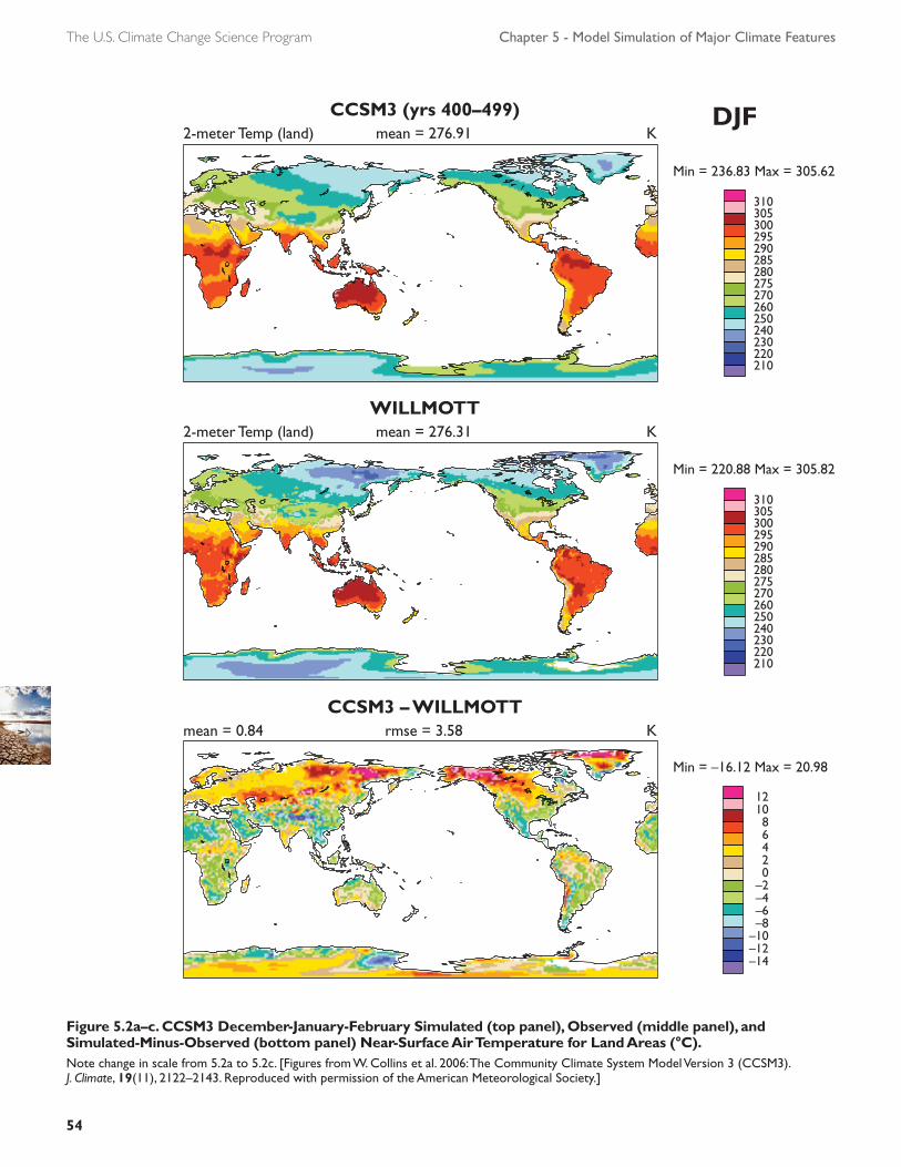
54

The U.S. Climate Change Science Program Chapter 5 - Model Simulation of Major Climate Features

Figure 5.2a–c. CCSM3 December-January-February Simulated (top panel), Observed (middle panel), andSimulated-Minus-Observed (bottom panel) Near-Surface Air Temperature for Land Areas (°C).Note change in scale from 5.2a to 5.2c. [Figures from W. Collins et al. 2006: The Community Climate System Model Version 3 (CCSM3).J. Climate, 19(11), 2122–2143. Reproduced with permission of the American Meteorological Society.]

CCSM3 – WILLMOTTmean = 0.84 rmse = 3.58 K

CCSM3 (yrs 400–499) DJF2-meter Temp (land) mean = 276.91 K

WILLMOTT2-meter Temp (land) mean = 276.31 K

Min = 236.83 Max = 305.62

Min = 220.88 Max = 305.82

Min = –16.12 Max = 20.98

310305300295290285280275270260250240230220210

310305300295290285280275270260250240230220210

121086420

–2–4–6–8

–10–12–14

55


5.2 TWENTIETH CENTURYTRENDS

Modern AOGCMs are able to simulate not onlythe time-average climate but also changes(trends) in climate over the past 140 years. Forexample, Fig. 5.3 shows results from the threeU.S. models and the “average” CMIP3 model.Plotted in the figure are curves of globally av-eraged annual mean near-surface temperaturefrom model simulations and the observationalvalue as determined from the U.K. Climatic Re-search Unit (CRU) gridded observational data-base. Two curves are plotted for the CMIP3models. The first shows the average over allCMIP3 models, and the second, the averageover only CMIP3 models that included the ef-fects of volcanic eruptions. Results from indi-vidual U.S. models are shown for separateensemble members (dotted lines) and for the av-erage over all ensemble members (continuouslines). Individual members of a particular modelensemble differ from each other because theywere run from different initial conditions. Pre-cise initial conditions, especially deep-ocean

temperature and salinity, are not known for1860. The spread among individual simulationsfrom the same model (the dotted-line curves)thus indicates uncertainty in model-simulatedtemperature arising from lack of knowledgeabout initial conditions.

These results demonstrate that modern climatemodels exhibit agreement with observed globalmean near-surface temperature trends to withinobservational uncertainty, despite imprecise ini-tial conditions and uncertain climate forcingand heat uptake by the deep ocean (Min andHense 2006). Models achieve this agreementonly if they include anthropogenic emissions ofgreenhouse gases and aerosols. No plausiblecombination of natural climate-forcing factorsallows models to explain the global warmingobserved over the last several decades. Indirectsolar effects [e.g., involving cosmic rays andclouds (Svensmark 2007)] are not generally in-cluded in AOGCM simulations. These effectshave been proposed occasionally as causes ofglobal warming, although over the past 20 yearstheir trends would, if anything, lead to cooling

Figure 5.2d. CCSM3 Annual Mean Simulated-Minus-Observed Sea SurfaceTemperature (°C). [Figure from W. Collins et al. 2006: The Community Climate System Model Version 3 (CCSM3). J. Climate,19(11), 2122–2143. Reproduced with permission of the American Meteorological Society.]

56


(Lockwood and Fröhlich 2007). Unless themodels grossly underestimate the climate sys-tem’s natural internally generated variability orare all missing a large unknown forcing agent,the conclusion is that most recent warming isanthropogenic (IPCC 2007b).

Nevertheless, total climate forcing during the20th Century is not accurately known, especiallythe aerosol component (see Chapter 2). Aerosolforcing used in these simulations, however, isderived from aerosol parameterizations con-strained by satellite and ground-based measure-ments of the aerosols themselves and was notdesigned to obtain a fit to observed global meantemperature trends. The observed trend in sur-face temperature can result from models withdifferent aerosol forcing (Schwartz 2007). Thus,20th Century temperature records cannot distin-guish models that would warm by differingamounts for the same total forcing.

Note that climate sensitivity is not prescribed inAOGCMs. Instead, this sensitivity emerges as aresult of a variety of lower-level modeling

choices. In contrast to simple energy-balancemodels that predict only the global mean tem-perature using a limited representation of cli-mate physics, an AOGCM’s climate sensitivityis difficult to specify a priori. More fundamen-tally, AOGCMs, unlike simpler climate models,have far fewer adjustable parameters than thenumber of observations available for modelevaluation (Randall et al. 2007). Thus, anAOGCM’s multidimensional output can becompared to observations independent of thisadjustment (e.g., using observed trends in re-gional temperature). Agreement between mod-eled and observed trends has been described fortemperature trends on each inhabited continent(Min and Hense 2007); for trends in climate ex-tremes, such as heat-wave frequency and frost-day occurrence (Tebaldi et al. 2006); and fortrends in surface pressure and Arctic sea ice (seeChapter 9 in IPCC 2007), all of which comple-ment comparisons between modeled and ob-served time-averaged climate discussed in thefollowing sections.

Figure 5.3a. Simulationof 20th CenturyGlobally AveragedSurface Temperaturefrom GFDL CM2.1.“CRU” is the value based onthe Climate Research Unitgridded observationaldataset, “IPCC Mean” is theaverage value of all CMIP3models, and “IPCC MeanVolc” is the average of allCMIP3 models that includedvolcanic forcing. Individualrealizations of the CMIP3 20th

Century experiment aredenoted by the dottedcurves labeled “run(1–3),”and the ensemble mean ismarked “Mean.”

1860

1870

1880

1890

1900

1910

1920

1930

1940

1950

1960

1970

1980

1990

2000

Time

-0.5

0

0.5

1

tas

IPCC Mean VolcIPCC Meanrun1run2run3MeanCR U

Global Warming relative to 1900 for gfdl_cm2_1 (10 years running average smoothed)

57


Figure 5.3b. Simulationof 20th CenturyGlobally AveragedSurface Temperaturefrom GISS Model E-R.Curve labels are the same asin Fig. 5.3a.

1860

1870

1880

1890

1900

1910

1920

1930

1940

1950

1960

1970

1980

1990

2000

Time

-0.5

0

0.5

1

tas

IPCC Mean VolcIPCC Meanrun1run2run3run4run5run6run7run8run9Mean

Global Warming relative to 1900 for giss_model_e_r (10 years running average smoothed)

CRU

Figure 5.3c. Simulationof 20th CenturyGlobally AveragedSurface Temperaturefrom CCSM3.Curve labels are the same asin Fig. 5.3a.

1860

1870

1880

1890

1900

1910

1920

1930

1940

1950

1960

1970

1980

1990

2000

Time

-0.5

0

0.5

1

tas

IPCC Mean VolcIPCC Meanrun1run2run3run4run5run6run7run9Mean

Global Warming relative to 1900 for ncar_ccsm3_0 (10 years running average smoothed)

CRU

Figure 5.3d.Comparison ofSimulations of 20th

Century GloballyAveraged SurfaceTemperature from theThree U.S. CMIP3Models. Model curves representensemble means for CCSM3(ncar_ccsm3_0), GISS ModelE-R (giss_e_r), and GFDLCM2.1 (gfdl_cm2_1). “CRU,”“IPCC Mean,” and “IPCCMean Volc” labels are thesame as in Fig. 5.3a.

1860

1870

1880

1890

1900

1910

1920

1930

1940

1950

1960

1970

1980

1990

2000

Time

-0.5

0

0.5

1

tas

IPCC Mean VolcIPCC Meangfdl_cm2_1

giss_model_e_r

ncar_ccsm3_0

Global Warming Relative to 1900 for American Models (10 years running average smoothed)

CRU

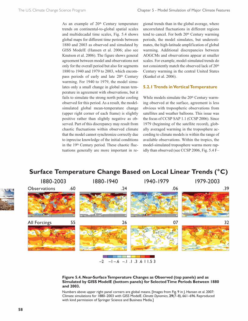
58


As an example of 20th Century temperaturetrends on continental-to-global spatial scalesand multidecadal time scales, Fig. 5.4 showsglobal maps for different time periods between1880 and 2003 as observed and simulated byGISS ModelE (Hansen et al. 2006; also seeKnutson et al. 2006). The figure shows generalagreement between model and observations notonly for the overall period but also for segments1880 to 1940 and 1979 to 2003, which encom-pass periods of early and late 20th Centurywarming. For 1940 to 1979, the model simu-lates only a small change in global mean tem-perature in agreement with observations, but itfails to simulate the strong north polar coolingobserved for this period. As a result, the model-simulated global mean-temperature change(upper right corner of each frame) is slightlypositive rather than slightly negative as ob-served. Part of this discrepancy may result fromchaotic fluctuations within observed climatethat the model cannot synchronize correctly dueto inprecise knowledge of the initial conditionsin the 19th Century period. These chaotic fluc-tuations generally are more important in re-

gional trends than in the global average, whereuncorrelated fluctuations in different regionstend to cancel. For both 20th Century warmingperiods, the model simulates, but underesti-mates, the high-latitude amplification of globalwarming. Additional discrepancies betweenAOGCMs and observations appear at smallerscales. For example, model-simulated trends donot consistently match the observed lack of 20th

Century warming in the central United States(Kunkel et al. 2006).

5.2.1 Trends in Vertical Temperature

While models simulate the 20th Century warm-ing observed at the surface, agreement is lessobvious with tropospheric observations fromsatellites and weather balloons. This issue wasthe focus of CCSP SAP 1.1 (CCSP 2006). Since1979 (beginning of the satellite record), glob-ally averaged warming in the troposphere ac-cording to climate models is within the range ofavailable observations. Within the tropics, themodel-simulated troposphere warms more rap-idly than observed (see CCSP 2006, Fig. 5.4 F–

Figure 5.4. Near-Surface Temperature Changes as Observed (top panels) and asSimulated by GISS ModelE (bottom panels) for Selected Time Periods Between 1880and 2003. Numbers above upper right panel corners are global means. [Images from Fig. 9 in J. Hansen et al. 2007:Climate simulations for 1880–2003 with GISS ModelE. Climate Dynamics, 29(7–8), 661–696. Reproducedwith kind permission of Springer Science and Business Media.]

Surface Temperature Change Based on Local Linear Trends (°C)1880-2003

Observations .601880-1940

.241940-1979

.061979-2003

.39

All Forcings 55 26 07 32

–2 –1 –.1 .1 .3 .6 1 1.5 3–.6

59


G). SAP 1.1 noted, however, that “Large struc-tural uncertainties in the observations . . . makeit difficult to reach more definitive conclusionsregarding the significance and importance ofmodel-data discrepancies” (CCSP 2006, p. 112and Section 5.4).

Research since publication of SAP1.1 has con-tinued to highlight uncertainties implicit inmeasuring the difference between surface andlower-atmospheric warming. For example,Thorne et al. (2007) found that the tropical at-mosphere-to-surface warming ratio in both ob-servations and model simulations is sensitive tothe time period analyzed. Meanwhile, debatecontinues over the best way to process data fromsatellites (Christy et al. 2007) and weather bal-loons (Christy and Spencer 2005). AOGCMscontinue to differ from most published obser-vations on the ratio of atmosphere-to-surfacewarming in the tropics since the beginning ofsatellite observations (e.g., as shown by Thorneet al. 2007, Fig. 3), with the ratio being larger inthe models than is seen in decadal observationaltrends.

Paradoxically, trends are more consistent be-tween models and observations on interannualtime scales. AOGCM simulation of tropical at-mospheric warming involves mainly subgrid-scale parameterizations. As discussed inChapter 2, these are not as trustworthy as ex-plicitly computed processes, but internal vari-ability [primarily due to El Niño–SouthernOscillation (ENSO)] provides a useful test ofthe models’ ability to redistribute heat realisti-cally. AOGCMs simulate very well the portionof tropical temperature trends due to interannualvariability (Santer et al. 2005). In addition, ex-plaining how atmospheric water vapor increasescoincidentally with surface temperature is dif-ficult (Trenberth, Fasullo, and Smith 2005; San-ter et al. 2007; Wentz et al. 2007) unless lowertropospheric temperature also increases coinci-dentally with surface temperature. While defi-ciencies in model subgrid-scale parameter-izations are certainly possible, trends in poorlydocumented forcing agents (see Chapter 4) mayprove important in explaining the discrepancyover the longer time scales. Future research isrequired to resolve the issue because tropos-pheric observations at face value suggest a trendtoward greater tropical instability, which has im-

plications for many aspects of model projec-tions in the tropics.

5.2.2 Model Simulation of ObservedClimate Variability

The following sections discuss a number of spe-cific climate phenomena directly or indirectlyrelated to near-surface temperature, precipita-tion, and sea level. Numerous studies of climatechange have focused on one or two of these phe-nomena, so a great deal of information (and oc-casional debate) has accumulated for each ofthem. Here we attempt to summarize the pointsthat would best give users of AOGCM modeloutput a general sense of model reliability orunreliability. Although the following sectionsindividually note different types of climate vari-ation, the reader should recognize that the totalamount of natural climate variability formsbackground “noise” that must be correctly as-sessed to identify the “signal” of anthropogenicclimate change. Natural variability in turn sep-arates into an externally forced part (e.g., fromsolar energy output and volcanic eruptions) andinternally generated variability just as weathervaries on shorter time scales because of the sys-tem’s intrinsic chaotic character. As notedabove, long-term trends in both solar and vol-canic forcing during the past few decades havehad a cooling rather than warming effect. It fol-lows that if global warming during this period isnot anthropogenic, then the climate system’s in-ternal variation is the most likely alternative ex-planation.

Control runs of AOGCMs (in which no changesin external climate forcing are included) provideestimates of the level of internally generated cli-mate variability. Control runs generally obtainrealistic near-surface temperature variability onannual-to-decadal time scales, although theytypically underestimate variability in areas ofthe Pacific and Indian Ocean where ENSO andthe Pacific Decadal Oscillation (PDO) (seebelow) predominate (Stouffer, Hegerl, and Tett2000). Unfortunately, the longest time periodsthat are directly relevant to separating naturalfrom anthropogenic climate change are the leastobserved. Assessing variations of surface tem-perature for time periods longer than 50 to 100years depends on paleodata such as ice-corecomposition and tree-ring thickness. Interpreta-

60


tion of these data is made difficult by sparse ge-ographical coverage and also is complicated bynatural variations in external climate forcing.

5.2.2.1 EXTRA-TROPICAL STORMS

Climate models have developed from numeri-cal weather-prediction models whose perform-ance has been judged primarily on their abilityto forecast midlatitude weather. The success offorecast models in their simulation of midlati-tude cyclones and anticyclones has resulted incontinuous growth in the value of numericalweather prediction. The ability of GCMs to gen-erate realistic statistics of midlatitude weatheralso has been central in climate model develop-ment. This is true not only because midlatitudeweather is important in its own right, but alsobecause these storms are the primary mecha-nism by which heat, momentum, and watervapor are transported by the atmosphere, mak-ing their simulation crucial for simulation ofglobal climate. Indeed, a defining feature of at-mospheric general circulation models(AGCMs) is that they compute midlatitude eddystatistics and associated eddy fluxes through ex-plicit computation of the life cycles of individ-ual weather systems and not through someturbulence or parameterization theory. Comput-ing the evolution of individual eddies may seemvery inefficient when primary interest is inlong-term eddy statistics, but the communityclearly has judged for decades that explicit eddysimulation in climate models is far superior toattempts to develop closure theories for eddystatistics. The latter theories typically form thebasis for Earth system models of intermediatecomplexity (EMICs), which are far more effi-cient computationally than GCMs but provideless convincing simulations.

Two figures illustrate the quality of simulatedmidlatitude eddy statistics from coupledAOGCMs used in IPCC AR4. Shown for theGFDL CM2.1 in Fig. 5.5a is wintertime vari-ance of the north-south velocity component at300 hPa (in the upper troposphere). This quan-tity represents the magnitude of variability inthe upper troposphere associated with day-to-day weather. In Fig. 5.5b, the wintertime pole-ward eddy heat flux or covariance betweentemperature and north-south velocity is shownat 850 mb (in the lower troposphere). For thesecalculations, the monthly means were sub-

tracted before computing variances. In eachcase, eddy statistics are compared to estimatesof observed statistics obtained fromNCEP/NCAR Reanalysis (B.Wyman, personalcommunication). When analyzing eddy statis-tics, the data are typically filtered to retain onlythose time scales, roughly 2 to 10 days, associ-ated with midlatitude weather systems. The twoquantities chosen here, however, are sufficientlydominated by these time scales that they are rel-atively insensitive to the monthly filtering usedhere. In winter, Northern Hemisphere stormsare organized into two major oceanic stormtracks over the Pacific and Atlantic oceans. His-torically, atmospheric models of horizontal res-olutions of 200 to 300 km typically are capableof simulating midlatitude storm tracks with re-alism comparable to that shown in the figure.Eddy amplitudes often are a bit weak and oftendisplaced slightly equatorward. In spectral mod-els with resolution coarser than 200 to 300 km,simulation of midlatitude storm tracks typicallydeteriorates significantly (see, e.g., Boyle1993). General improvements in most modelsin the CMIP3 database over previous genera-tions of models, as described in Chapter 1, arethought to be partly related to the fact that mostof these models now have grid sizes of 100 to300 km or smaller. Although even-finer resolu-tion results in better simulations of midlatitude-storm structure, including that of warm and coldfronts and interactions among these storms andcoastlines and mountain ranges, improvementsin midlatitude climate on large scales tend to beless dramatic and systematic. Other factors be-sides horizontal resolution are considered im-portant for details of storm track structure. Suchfactors include distribution of tropical rainfall,which is sensitive to parameterization schemesused for moist convection, and interactions be-tween stratosphere and troposphere, which aresensitive to vertical resolution. Roeckner et al.(2006), for example, illustrate the importanceof vertical resolution for midlatitude circulationand storm track simulation.

Lucarini et al. (2006) provide a more detailedlook at the ability of CMIP3 models to simulatethe space-time spectra of observed eddy statis-tics. These authors view the deficiencies noted,which vary in detail from model to model, asserious limitations to model credibility. As in-dicated in Chapter 1, however, our ability is lim-

61


ited in translating measures of model biases intouseful measures of model credibility for 21st

Century projections, and the implications ofthese biases in eddy space-time spectra are notself-evident. Indeed, in the context of simulatingeddy characteristics generated in complex tur-bulent flows in the laboratory (e.g., Pitsch2006), the quality of atmospheric simulations,based closely on fluid dynamical first princi-ples, probably should be thought of as one ofthe most impressive characteristics of currentmodels. As an example of a significant modeldeficiency that plausibly can be linked to limi-

tations in climate projection credibility, notethat the Atlantic storm track, as indicated by themaximum velocity variance in Fig. 5.5a, followsa latitude circle too closely and the observedstorm track has more of a southwest-northeasttilt. This particular deficiency is common inCMIP3 models (van Ulden and van Oldenborgh2006) and is related to difficulty in simulatingthe blocking phenomenon in the North Atlanticwith correct frequency and amplitude. VanUlden and van Oldenborgh make the case thatthis bias is significant for the quality of regionalclimate projections over Europe.

DJF 300 hPa v' v'(m2s–2)CM2.1_AllForc_H2 (1981 – 2000)max = 337.5

min = 2.989avg = 88.05std = 72.62

max = 85.53min = –118

avg = –7.245rms = 24.45

max = 358.4min = 5.79

avg = 95.3std = 78.99NCEP (1981 – 2000)

CM2.1_AllForc_H2 – NCEP

80°N

40°N

0°

40°S

80°S

400

350

300

250

200

150

100

50

0

80°N

40°N

0°

40°S

80°S

400

350

300

250

200

150

100

50

0

80°N

40°N

0°

40°S

80°S

125100

755025

0–25–50–75

–100–125

50°E 150°E 110°W 10°W

50°E 150°E 110°W 10°W

50°E 150°E 110°W 10°W

Figure 5.5a. Top:Variance of North-South Velocity at 300hPa as Simulated byGFDL CM2.1 Model inYears 1981 to 2000 ofOne Realization of20C3M Simulation, asContributed to theCMIP3 Database. Units are m2/s2. Middle:Same quantity as obtainedfrom NCEP/NCARReanalysis (Kalnay et al.1996). Bottom: Model minusobservations.

62


5.2.2.2 TROPICAL STORMS

Tropical storms (hurricanes in the Atlantic andtyphoons in the Pacific and Indian oceans) aretoo small to be simulated reliably in the class ofglobal-climate models currently used for cli-mate projections. There is hope for simulatingregional climate aspects that control the gene-sis of tropical depressions, however. Vitart andAnderson (2001), for example, identified trop-ical storm-like vortices in simulations withmodels of this type, demonstrating some skill

in simulating the effects of El Niño on Atlanticstorm frequency.

Simulations with atmospheric models aresteadily moving to higher resolutions (e.g.,Bengtsson, Hodges, and Esch 2007). The recent20-km–resolution simulation with an atmos-pheric model over prescribed ocean tempera-tures by Oouchi et al. (2006) is indicative of thekinds of modeling that will be brought to bearon this problem in the next few years. Experi-

DJF 850 hPa v' T' (m° K s –1)CM2.1_AllForc_H2 (1981 – 2000)max = 32.27

min = 14.85avg = 2.3

std = 8.24

max = 18.4min = –11.78

avg = 0.9021rms = 2.588

max = 32.38min = 17.59

avg = 1.398std = 7.577NCEP (1981 – 2000)

CM2.1_AllForc_H2 – NCEP

80°N

40°N

0°

40°S

80°S

40353025201510

50

–5–10–15–20–25–30–35–40

80°N

40°N

0°

40°S

80°S

40353025201510

50

–5–10–15–20–25–30–35–40

80°N

40°N

0°

40°S

80°S

211812

9630

–3–6–9

–12–15–18–21

50°E 150°E 110°W 10°W

50°E 150°E 110°W 10°W

50°E 150°E 110°W 10°W

Figure 5.5b. Top:Covariance of North-South Velocity andTemperature at 850hPa as Simulated byGFDL CM2.1 Model inYears 1981 to 2000 ofOne Realization of20C3M Simulation, asContributed to theCMIP3 Database. Units are K-m/s. Middle:Same quantity as obtainedfrom NCEP/NCARReanalysis (Kalnay et al.1996). Bottom: Model minusobservations.

63


ence with tropical storm forecasting suggeststhat this resolution should be adequate for de-scribing many aspects of the evolution of ma-ture tropical storms and possibly the generationof storms from incipient disturbances, but prob-ably not tropical storm intensity. A promisingalternative approach is described by Knutson etal. (2007), in which a regional model of com-parable resolution (18 km) is used in a down-scaling framework (see Chapter 3) to simulatethe Atlantic hurricane season. Given observedyear-to-year variations in the large-scale atmos-phere structure over the Atlantic Ocean, themodel is capable of simulating year-to-yearvariations in hurricane frequency over a 30-yearperiod with a correlation of 0.7 to 0.8. It alsocaptures the observed trend toward greater hur-ricane frequency in the Atlantic during this pe-riod. These results suggest that downscalingusing models of this resolution may be able toprovide a convincing capability for tropicalstorm frequency projections into the future, al-though these projections still will rely on thequality of global model projections for changesin sea-surface temperature, atmospheric stabil-ity, and vertical shear.

5.2.2.3 MONSOONS

A monsoonal circulation is distinguished by itsseasonal reversal after the sun crosses the equa-tor into the new summer hemisphere. Rain ismost plentiful in, if not entirely restricted to,summer within monsoonal climates, when con-tinental rainfall is supplied mainly by evapora-tion from the nearby ocean. This limits the reachof monsoon rains to the distance over whichmoisture can be transported onshore (Privé andPlumb 2007). Variations in the monsoon’s spa-tial extent from year to year determine whichinland regions experience drought.

Over a billion people are dependent on the ar-rival of monsoon rains for water and irrigationfor agriculture. The Asian monsoon during bo-real summer is the most prominent example ofa monsoon circulation dominating global rain-fall during this season. However, the summerrainfall maximum and seasonal reversal ofwinds also indicate monsoon circulations inWest Africa and the Amazon basin. In addition,during boreal summer, air flows off the easternPacific Ocean toward Mexico and the AmericanSouthwest while, over the Great Plains, mois-

ture from the Gulf of Mexico brings an annualpeak in rainfall. Thus, the climate in these re-gions also is described as monsoonal.

Because of the Asian monsoon’s geographicalextent, measures of the fidelity of Asian mon-soonal simulations can differ depending on spe-cific regional focus and the metrics being used.Kripalani et al. (2007) judged that 3/4 of the 18analyzed coupled models match the timing andmagnitude of the summertime peak in precipi-tation over East Asia between 100 and 145°Eand 20 to 40°N evident in the NOAA-NCEPClimate Prediction Center’s Merged Analysis ofPrecipitation (CMAP, Xie, and Arkin 1997).However, only half of these models were able toreproduce the gross observed spatial distribu-tion of monsoon rainfall and its migration alongthe coast of China toward the Korean peninsulaand Japan. Considering a broader range of lon-gitude (40 to 180°E) that includes the Indiansubcontinent, Annamalai, Hamilton, and Sper-ber (2007) found that 6 of 18 AOGCMs signif-icantly correlated with the observed spatialpattern of CMAP precipitation from Junethrough September. (These six models also pro-duced relatively realistic simulation of ENSOvariability, which is known to influence inter-annual variations in the Asian summer mon-soon.) Kitoh and Uchiyama (2006) computedthe spatial correlation and root-mean-squareerror of simulated precipitation over a similarregion and found, for example, the GFDL mod-els in the top tercile with a spatial correlationexceeding 0.8.

During boreal winter, Asian surface winds aredirected offshore: from the northeast over Indiaand the northwest over East Asia. Hori andUeda (2006) provide correlations between ob-served spatial distributions of surface pressuresand 850-mb zonal winds during the East Asianwinter monsoon with winds and pressures sim-ulated by nine CMIP3 models. Correlations forzonal winds, for example, vary from 0.96 to0.75. Monsoonal simulations in these modelsclearly vary considerably in quality, more soperhaps than other circulation features. Ob-served year-to-year variability of the WestAfrican monsoon is related to remote oceantemperatures in the North and South Atlanticand Indian oceans (Rowell et al. 1992; Zhangand Delworth 2006) as well as to temperatures

64


in the nearby Gulf of Guinea. Cook and Vizy(2006) found that slightly more than half of 18analyzed coupled models reproduced the ob-served precipitation maximum over land fromJune through August. Of these models, only six(including GISS ModelE-H and both GFDLmodels) reproduced the observed anticorrela-tion between Gulf of Guinea ocean temperatureand Sahel rainfall.

The late 20th Century Sahel drought was a dra-matic change in the Earth’s hydrological cyclethat plausibly must be simulated by climatemodels if we are to have any confidence in theirability to project future climate in this region.Atmospheric models, when run over observedoceanic temperatures, simulate this drought rea-sonably well (Hoerling et al. 2006). In thesemodels, the drought is at least partly forced bywarming of the Northern Hemisphere oceans,particularly the North Atlantic, with respect toSouthern Hemisphere oceans, especially the In-dian Ocean and Gulf of Guinea. Although theconsensus is that these variations in ocean tem-perature gradients are at least partly due to nat-ural variability, they may have been partlyanthropogenically forced. Analysis of CMIP3simulations of the 20th Century by Biasutti andGiannini (2006), supporting the earlier model-ing study of Rotstayn and Lohmann (2002),suggests that aerosol forcing in these modelsplayed a part in generating this drought by cool-ing the North Atlantic with respect to otherocean basins. A small number of coupled mod-els simulate droughts of the observed magni-tude, including GFDL models (Held and Soden2006), but why some models are more realisticin this regard than others is not understood.

Rainfall over the Sahel and Amazon are anti-correlated: when the Gulf of Guinea warms,rainfall generally is reduced over the Sahel butincreases over South America. Amazon rainfallalso depends on the eastern equatorial Pacific,and, during an El Niño, rainfall is reduced in theNordeste region of the Amazon. Li et al. (2006)compare the hydrological cycle of 11 CGCMsover the Amazon during the late 20th and 21st

centuries. Based on a comparison to CMAPrainfall, the GISS ModelE-R is among the best.

The ability of climate models to simulate North-ern Hemisphere summer rainfall over the U.S.

Great Plains and Mexico was summarized byRuiz-Barradas and Nigam (2006). Models gen-erally have more difficulty in simulating sum-mer rainfall in the Great Plains than winterrainfall, and this disparity probably should bethought of as reflecting the quality of futurerainfall projections as well. Strengths and weak-nesses vary considerably across the models. Asan example, GISS ModelE-H closely matchesthe annual precipitation cycle over the GreatPlains and Mexico and is one of two models tosimulate interannual precipitation variationssignificantly correlated with observed variabil-ity during the second half of the 20th Century.

Initial monsoon evaluations simulated by themost recent generation of climate models haveemphasized the seasonal time scale. However,subseasonal variations, such as break periodswhen the monsoon rains are interrupted tem-porarily, are crucial to forecasting the mon-soon’s impact on water supply. Simulating thediurnal cycle and the local hour of rainfall alsois important to partitioning rainfall betweenrunoff and transpiration, and these are impor-tant topics for future model evaluation. Trans-ports of moisture by regional circulationsbeneath model resolution (such as low-level jetsalong the Rockies and Andes and tropical cy-clones) contribute to the onshore transport ofmoisture. In general, models show some successat simulating gross seasonal features of variousmonsoon circulations, but studies are limited onvariations of the smaller spatial and time scalesimportant to specific watersheds and hydrolog-ical projections.

5.2.2.4 MADDEN-JULIAN OSCILLATIONS

The Madden-Julian Oscillation (MJO) consistsof large-scale eastward-propagating patterns inhumidity, temperature, and atmospheric circu-lation that strengthen and weaken tropical rain-fall as they propagate around the Earth inroughly 30 to 60 days. This pattern often domi-nates tropical precipitation variability on timescales longer than a few days and less than aseason, creating such phenomena as 1- to 2-week breaks in Asian monsoonal rainfall andweeks with enhanced hurricane activity in theeastern North Pacific and the Gulf of Mexico.Inadequate prediction of the evolution of thesepropagating structures is considered a main im-pediment to more useful extended-range

65


weather forecasts in the tropics, and improvedsimulation of this phenomenon is considered animportant metric for the credibility of climatemodels in the tropics.

Nearly all models capture the pattern’s essentialfeature, with large-scale eastward propagationand with roughly the correct vertical structure.But propagation often is too rapid and ampli-tudes too weak. Recent surveys of model per-formance indicate that simulations of MJOremain inadequate. For example, Lin et al.(2006), in a study of many CMIP3 models, con-clude that “… current GCMs still have signifi-cant problems and display a wide range of skillin simulating the tropical intraseasonal vari-ability,” while Zhang et al. (2005) in anothermultimodel comparison study, state that “…commendable progress has been made in MJOsimulations in the past decade, but the modelsstill suffer from severe deficiencies ….” As anexample of recent work, Boyle et al. (2008) at-tempted, with limited success, to determinewhether two U.S. CMIP3 models could main-tain a preexisting strong MJO pattern when ini-tialized with observations [from the TropicalOcean Global Atmosphere–Coupled Ocean At-mosphere Response Experiment (called TOGA-COARE) field experiment].

The difficulty in simulating MJO is related tothe phenomenon’s multiscale nature: the propa-gating pattern itself is large enough to be re-solvable by climate models, but the convectionand rainfall modulated by this pattern, whichfeed back on the large-scale environment, occuron much smaller, unresolved scales. In additionto this dependence on parameterization of trop-ical convection, a long list of other effects hasbeen shown by models and observational stud-ies to be important for MJO. These effects in-clude the pattern of evaporation generated asMJO propagates through convecting regions,feedback from cloud-radiative interactions, in-traseasonal ocean temperature changes, the di-urnal cycle of convection over the ocean, andthe vertical structure of latent heating , espe-cially the proportion of shallow cumulus con-gestus clouds and deep convective cores indifferent phases of oscillation (Lin et al. 2004)].

A picture seems to be emerging that simulationdifficulty may not be due to a single model de-

ficiency but is a result of the phenomenon’scomplexity, given the long list of factors thoughtto be significant. In several multimodel studiessuch as Lin et al. (2006), a few models do per-form well. However, without a clearer under-standing of how these factors combine togenerate the observed characteristics of MJO,maintaining a good simulation when the modelis modified for other reasons is difficult, as isapplying the understanding gained from onemodel’s successful simulation to other models.Whether models with superior MJO simulationsshould be given extra weight in multimodelstudies of tropical climate change is unclear.

5.2.2.5 EL NIÑO–SOUTHERN OSCILLATION

By the mid-20th Century, scientists recognizedthat a local anomaly. in rainfall and oceanic up-welling near the coast of Peru was in fact part ofa disruption to atmospheric and ocean circula-tions across the entire Pacific basin. During ElNiño, atmospheric mass migrates west of thedateline as part of the Southern Oscillation, re-ducing surface pressure and drawing rainfallinto the central and eastern Pacific (Rasmussenand Wallace 1983). Together, El Niño and theSouthern Oscillation, abbreviated in combina-tion as ENSO, are the largest source of tropicalvariability observed during recent decades. Be-cause of the Earth’s rotation, easterly windsalong the equator cool the surface by raisingcold water from below, which offsets heating bysunlight absorption (e.g., Clement et al. 1996).Cold water is especially close to the surface inthe east Pacific, while warm water extendsdeeper in the west Pacific so upwelling has lit-tle effect on surface temperature there. Thewestward increase in temperature along theequator is associated with a decrease in atmos-pheric pressure, reinforcing the easterly tradewinds. El Niño occurs when easterly tradewinds slacken, reducing upwelling and warm-ing the ocean surface in the central and east Pa-cific.

Changes along the equatorial Pacific have beenlinked to global disruptions of climate (Ro-pelewski and Halpert 1987). During an El Niñoevent, the Asian monsoon typically is weakened,along with rainfall over eastern Africa, whileprecipitation increases over the AmericanSouthwest. El Niño raises the surface tempera-ture as far poleward as Canada, while changes

66


in the north Pacific Ocean are linked to decadalvariations in ENSO (Trenberth and Hurrell1994). In many regions far from eastern equa-torial Pacific, accurate projections of climatechange in the 21st Century depend upon the ac-curate projection of changes to El Niño. More-over, the demonstration that ENSO altersclimate across the globe indicates that evenchanges to the time-averaged equatorial Pacificduring the 21st Century will influence climatefar beyond the tropical ocean. For example,long-term warming of the eastern equatorial Pa-cific relative to the surrounding ocean will favora weaker Asian monsoon year after year, evenin the absence of changes to the size and fre-quency of El Niño events.

In general, coupled models developed forCMIP3 are far more realistic than those of adecade ago, when ENSO variability was com-paratively weak and some models lapsed intopermanent El Niño states (Neelin et al. 1992).Even compared to models assessed more re-cently by the El Niño Simulation Intercompar-ison Project (called ENSIP) and CMIP2 (Latifet al. 2001; AchutaRao and Sperber 2002),ENSO variability of ocean surface temperatureis more realistic in CMIP3 simulations, al-though sea-level pressure and precipitationanomalies show little recent improvement(AchutaRao and Sperber 2006). Part of thisprogress is the result of increased resolution ofequatorial ocean circulation that has accompa-nied increases in computing speed. Table 5.1shows horizontal and vertical resolution near

the equator in oceanic components of the sevenAmerican coupled models whose output wassubmitted to CMIP3.

Along the equator, oceanic waves that adjust theequatorial temperature and currents to changesin the wind are confined tightly to within a fewdegrees of latitude. To simulate this adjustment,the ocean state is calculated at points as closelyspaced as 0.27 degrees of latitude in the NCARCCSM3. NCAR PCM has a half-degree resolu-tion, while both GFDL models have equatorialresolution of a third of a degree. This degree ofdetail is a substantial improvement compared toprevious generations of models. In contrast, theGISS AOM and ModelE-R calculate equatorialtemperatures at grid points separated by four de-grees of latitude. This is broad compared to thelatitudinal extent of cold temperatures observedwithin the eastern Pacific. The cooling effect ofupwelling is spread over a larger area, so theamplitude of the resulting surface temperaturefluctuation is weakened. In fact, both the GISSAOM models and ModelE-R have unrealisticENSO variations that are much smaller than ob-served (Hansen et al. 2007). This minimizes theinfluence of their simulated El Niño and LaNiña events on climate outside the equatorialPacific, and we will not discuss these two mod-els further in this section.

In comparison to previous generations of globalmodels, where ENSO variability was typicallyweak (Neelin et al. 1992), the AR4 coupledmodels generally simulate El Niño near the ob-served amplitude or even above (AchutaRaoand Sperber 2006). The latter study comparedsea-surface temperature (SST) variability withinthe tropical Pacific, calculated under preindus-trial conditions. Despite its comparatively lowtwo-degree latitudinal grid spacing, the GISSModelE-H (among American models) mostclosely matches observed SST variability sincethe mid-19th Century, according to the HadISSTv1.1 dataset (Rayner et al. 2003). The NCARPCM also exhibits El Niño warming close to theobserved magnitude. This comparison is basedon spatial averages within three longitudinalbands, and GISS ModelE-H, along with NCARmodels, exhibits its largest variability in theeastern band as observed. However, GISS Mod-elE-H underestimates variability since 1950,when the NCAR CCSM3 is closest to observa-

MODEL Longitude Latitude VerticalLevels

GFDL CM2.0 1 1/3 50

GFDL CM2.1 1 1/3 50

GISS AOM 5 4 13

GISS ModelE-H 2 2 16

GISS ModelE-R 5 4 13

NCAR CCSM3 1.125 0.27 27

NCAR PCM 0.94 0.5 32

*Except for GISS models, spacing of grid pointsgenerally increases away from the equator outsidethe ENSO domain, so resolution is highest at theequator.

Table 5.1. Spacingof Grid Points atthe Equator in theAmericanCoupled ModelsDeveloped forAR4*

67


tions (Joseph and Nigam 2006). Although thefidelity of each model’s ENSO variability de-pends on the specific dataset and period of com-parison (c.f. Capotondi, Wittenberg, and Masina2006; Merryfield 2006; van Oldenborgh, Philip,and Collins 2005), the general consensus is thatGISS ModelE-H, both NCAR models, andGFDL CM2.0 have roughly the correct ampli-tude, while variability is too large by roughlyone-third in GFDL CM2.1. Most models (in-cluding GISS ModelE-H and both NCAR mod-els but excluding GFDL models) exhibit thelargest variability in the eastern band of longi-tude, but none of the CMIP3 models matchesthe observed variability at the South Americancoast where El Niño was identified originally(AchutaRao and Sperber 2006; Capotondi, Wit-tenberg, and Masina 2006). This possibly is be-cause the longitudinal spacing of model grids istoo large to resolve coastal upwelling and its in-terruption during El Niño (Philander andPacanowski 1981). Biases in atmospheric mod-els (e.g., underestimating persistent stratuscloud decks along the coast) also may con-tribute (Mechoso et al. 1995).

El Niño occurs every few years, albeit irregu-larly. The spectrum of anomalous ocean tem-perature shows a broad peak between 2 and 7years, and multidecadal variations occur inevent frequency and amplitude. Almost all AR4models have spectral peaks within this range oftime scales. Interannual power is distributedbroadly within the American models, as ob-served, with the exception of NCAR CCSM3,which exhibits strong biennial oscillations(Guilyardi 2006).

Although models generally simulate the ob-served magnitude and frequency of events, re-producing their seasonality is more elusive.Anomalous warming typically peaks late in thecalendar year, as originally noted by SouthAmerican fisherman. Among American mod-els, this seasonal dependence is simulated onlyby NCAR CCSM3 (Joseph and Nigam 2006).Warming in GFDL CM2.1 and GISS ModelE-H is nearly uniform throughout the year, whilewarming in NCAR PCM is largest in Decem-ber but exhibits a secondary peak in early sum-mer. The mean seasonal cycle along theequatorial Pacific also remains a challenge forthe models. Each year, the east Pacific cold

tongue is observed to warm during borealspring and cool again late in the calendar year.GFDL CM2.1 and NCAR PCM1 have theweakest seasonal cycle among American mod-els, while GISS ModelE-H, GFDL 2.0, andNCAR CCSM3 are closest to the observed am-plitude (Guilyardi 2006). Among the worldwidesuite of CMIP3 models, amplitude of the sea-sonal cycle of equatorial ocean temperaturegenerally varies inversely with the ENSOcycle’s strength.

Several studies have compared mechanismsgenerating ENSO variability in CMIP3 modelsto those inferred from observations (e.g., vanOldenborgh, Philip, and Collins 2005; Guilyardi2006; Merryfield 2006; Capotondi, Wittenberg,and Masina 2006). Models must simulate thechange in ocean upwelling driven by changes insurface winds, which in turn are driven by re-gional contrasts in ocean temperature. In gen-eral, GFDL2.1 is ranked consistently amongAmerican models as providing the most realis-tic simulation of El Niño. This is not based pri-marily on its surface-temperature variability(which is slightly too large) but on its faithfulsimulation of the observed relationship betweenocean temperature and surface wind, along withwind-driven ocean response. While SST vari-ability in CMIP3 models is controlled by anom-alies of either upwelling rate or temperature,these processes alternate in importance overseveral decades within GFDL CM2.1 as ob-served (Guilyardi 2006). Since the 1970s theupwelling temperature, rather than the rate, hasbeen the predominant driver of SST variability(Wang 1995). A confident prediction of futureEl Niño amplitude requires both the upwellingrate and temperature, along with their relativeamplitude, to be simulated correctly. This re-mains a challenge.

El Niño events are related to climate anomaliesthroughout the globe. Models with more realis-tic ENSO variability generally exhibit an anti-correlation with the strength of the Asiansummer monsoon (e.g., Annamalai, Hamilton,and Spencer 2007), while 21st Century changesto Amazon rainfall have been shown to dependon projected trends in the tropical Pacific (Li etal. 2006). El Niño has a long-established rela-tion to North American climate (Horel and Wal-lace 1981), assessed in CMIP3 models by

68


Joseph and Nigam (2006). This relation isstrongest during boreal winter, when tropicalanomalies are largest. Anomalous circulationsdriven by rainfall over the warming equatorialCentral Pacific radiate atmospheric distur-bances into midlatitudes amplified within thenorth Pacific storm track (Sardeshmukh andHoskins 1988; Held, Lyons, and Nigam 1989;Trenberth et al. 1998). To simulate ENSO’s in-fluence on North America, models must repre-sent realistic rainfall anomalies in the correctseason so the connection is amplified by win-tertime storm tracks. The connection betweenequatorial Pacific and North American climateis simulated most accurately by the NCARPCM model (Joseph and Nigam 2006). InGFDL CM2.1, North American anomalies aretoo large, consistent with the model’s excessiveEl Niño variability within the equatorial Pacific.The connection between the two regions is re-alistic if the model’s tropical amplitude is ac-counted for. In the GISS model, anomalousrainfall during ENSO is small, consistent withthe weak tropical wind stress anomaly citedabove. The influence of El Niño over NorthAmerica is nearly negligible in this model. Theweak rainfall anomaly presumably is a result ofunrealistic coupling between atmospheric andocean physics. When SST instead is prescribedin this model, rainfall calculated by the GISSModelE AGCM over the American Southwestis significantly correlated with El Niño as ob-served.

Realistic simulation of El Niño and its globalinfluence remains a challenge for coupled mod-els because of myriad contributing processesand their changing importance in the observa-tional record. Key aspects of coupling betweenocean and atmosphere—the relation betweenSST and wind stress anomalies, for example—are the result of complicated interactions amongresolved model circulations, along with para-meterizations of ocean and atmospheric bound-ary layers and moist convection. Simple modelsidentify parameters controlling the magnitudeand frequency of El Niño, such as the windanomaly resulting from a change in SST (e.g.,Zebiak and Cane 1987; Fedorov and Philander2000), offering guidance to improve the realismof fully coupled GCMs. However, in a GCM,the coupling strength is emergent rather thanprescribed, and it is often unclear a priori how to

change the coupling. Nonetheless, improvedsimulations of the ENSO cycle compared toprevious generations (AchutaRao and Sperber2006) suggest that additional realism can be ex-pected in the future.

5.2.2.6 ANNULAR MODES

The primary mode of Arctic interannual vari-ability is the Arctic Oscillation (Thompson andWallace 1998), which also is referred to as thenorthern annular mode (NAM) and is related tothe North Atlantic Oscillation (Hurrell 1995).The primary mode of Antarctic interannual vari-ability is the southern annular mode (SAM)(Thompson and Wallace 2000), also known asAntarctic Oscillation. The variability modes areparticularly important for attributing and pro-jecting climate change; observed circulationchanges in the past few decades (especially inthe Southern Hemisphere) and model-projectedchanges in future circulation strongly resemblethese structures.

Coupled climate models have shown skill insimulating NAM (Fyfe, Boer, and Flato 1999;Shindell et al. 1999; Miller, Schmidt, and Shin-dell 2006). In some cases, too much variabilityin the simulation of sea-level pressure is asso-ciated with NAM (Miller, Schmidt, and Shin-dell 2006). Global climate models alsorealistically simulate SAM (Fyfe, Boer, andFlato 1999; Cai, Whetton, and Karoly 2003;Miller, Schmidt, and Shindell 2006), althoughsome details of SAM (e.g., amplitude and zonalstructure) show disagreement among global cli-mate model simulations and reanalysis data(Raphael and Holland 2006; Miller, Schmidt,and Shindell 2006).

In response to increasing concentrations ofgreenhouse gases and tropospheric sulfateaerosols in the 20th Century, the multimodel av-erage exhibits a positive trend in the annularmode index in both hemispheres, with decreas-ing sea-level pressure over the poles and a com-pensating increase in midlatitudes mostapparent in the Southern Hemisphere (Miller,Schmidt, and Shindell 2006). A variety of mod-eling studies also have shown that trends instratospheric climate can affect the tropos-phere’s annular modes (Shindell et al. 1999). In-deed, an important result from atmosphericmodeling in recent years is the realization that

69


the stratospheric ozone hole has contributed sig-nificantly to observed trends in surface windsand sea-level pressure distribution in the South-ern Hemisphere (Thompson and Solomon2002; Gillett and Thompson 2003). The mod-els, however, may not be trustworthy in theirsimulation of the relative magnitude of green-house gas and stratospheric ozone effects on theannular mode. They also may underestimate thecoupling of stratospheric changes due to vol-canic aerosols with annular surface variations(Miller, Schmidt, and Shindell 2006; Arblasterand Meehl 2006).

5.2.2.7 OTHER MODES OF MULTIDECADAL

VARIABILITY

In the Arctic during the last century, two long-period warm events occurred, one between 1920and 1950 and another beginning in the late1970s. Wang et al. (2007) evaluated a set ofCMIP3 models for their ability to reproduce theamplitudes of air temperature variability of thischaracter. As examples, CCSM3 and GFDL-CM2 models contain variance similar to that ob-served in the Arctic region.

Multidecadal variability in the North Atlantic ischaracterized by the Atlantic Multidecadal Os-cillation (AMO) index, which represents a spa-tial average of SST (Enfield, Mestas-Nuñez,and Trimble 2001). Kravtsov and Spannagle(2007) analyzed SST from a set of current gen-eration climate models. Their analysis attemptsto separate variability associated with internalocean fluctuations from that associated withchanges by anthropogenic contributions. Byisolating the multidecadal period of several re-gions in the ensemble SST series through sta-tistical methods, they found that models obtainthe observed magnitude of the AMO (Kravtsovand Spannagle 2007).

In the midlatitude Pacific region, decadal vari-ability generally is underrepresented in theocean (e.g., volume transports as described byZhang and McPhaden 2006), with some mod-els approaching amplitudes seen in observa-tions. Examination of complicated feedbacksbetween atmosphere and ocean at decadal andlonger scales shows that, while climate modelsgenerally reproduce the SST pattern related tothe Pacific Decadal Oscillation (PDO), ob-served correlations between PDO and tropical

SST are not seen in the models (e.g., Alexanderet al. 2006).

One of the most difficult areas to simulate is theIndian Ocean because of the competing effectsof warm water inflow through the Indonesianarchipelago, ENSO, and monsoons. Theprocesses interact to varying degrees, challeng-ing a model’s ability to simulate all system as-pects with observed relative emphasis. An indexused to understand variability is the IndianOcean Dipole pattern that combines informa-tion about SST and wind stress fields (Saji et al.1999). While most models evaluated by Saji,Xie, and Yamagata (2005) were able to simulatethe Indian Ocean’s response to local atmos-pheric forcing in short time periods (semian-nual), longer-period events such as the ocean’sresponse to ENSO changes in the Pacific werenot simulated well.

5.2.3 Polar Climates

Changes in polar snow and ice cover affect theEarth’s albedo and thus the amount of insola-tion heating the planet (e.g., Holland and Bitz2003; Hall 2004; Dethloff et al. 2006). Meltingglaciers and ice sheets in Greenland and westernAntarctica could produce substantial sea-levelrise (Arendt et al. 2002; Braithwaite and Raper2002; Alley et al. 2005). Polar regions thus re-quire accurate simulation for projecting futureclimate change and its impacts.

Polar regions present unique environments and,consequently, challenges for climate modeling.Key processes include sea ice, seasonally frozenground, and permafrost (Lawrence and Slater2005; Yamaguchi, Noda, and Kitoh 2005).Processes also include seasonal snow cover(Slater et al. 2001), which can have significantsubgrid heterogeneity (Liston 2004), and clear-sky precipitation, especially in the Antarctic(King and Turner 1997; Guo, Bromwich, andCassano 2003). Polar regions test the ability ofmodels to handle extreme geophysical behaviorsuch as longwave radiation in clear, cold envi-ronments (Hines et al. 1999; Chiacchio, Fran-cis, and Stackhouse 2002; Pavolonis, Key, andCassano 2004) and cloud microphysics in therelatively clean polar atmosphere (Curry et al.1996; Pinto, Curry, and Intrieri 2001; Morrisonand Pinto 2005). In addition, polar atmospheric

70


boundary layers can be very stable (Duynkerkeand de Roode 2001; Tjernström, Zagar, andSvensson 2004; Mirocha, Kosovic, and Curry2005), and their simulation remains an impor-tant area for model improvement.

For polar regions, much of simulated-variabilityassessment has focused on primary modes ofpolar interannual variability, along with thenorthern and southern annular modes. Less at-tention has been given to the ability of globalclimate-system models to simulate shorter-du-ration climate and weather variability in polarregions. Uotila et al. (2007) and Cassano et al.(2007) evaluated the ability of an ensemble of15 global climate-system models to simulatedaily variability in sea-level pressure in theAntarctic and Arctic. In both polar regions, theyfound that the ensemble was not able to repro-duce many features of daily synoptic climatol-ogy, with only a small subset of modelsaccurately simulating the frequency of primarysynoptic weather patterns identified in globalreanalysis datasets. U.S. models discussed in de-tail in Chapter 2 of this report spanned the samerange of accuracy as non-U.S. models, withGFDL and CCSM models part of a small, ac-curate subset. More encouraging results wereobtained by Vavrus et al. (2006), who assessedthe ability of seven global climate models tosimulate extreme cold-air outbreaks in theNorthern Hemisphere.

Attention also has been given to the ability ofregional climate models to simulate polar cli-mate. In particular, the Arctic Regional ClimateModel Intercomparison Project (ARCMIP) en-gaged a suite of Arctic regional atmosphericmodels to simulate a common domain and pe-riod over the western Arctic (Curry and Lynch2002). Rinke et al. (2006) evaluated spatial andtemporal patterns simulated by eight ARCMIPmodels and found that the model ensembleagreed well with global reanalyses, despitesome large errors for individual models. Tjern-strom et al. (2005) evaluated near-surface prop-erties simulated by six ARCMP models. Ingeneral, surface pressure, air temperature, hu-midity, and wind speed all were well simulated,as were radiative fluxes and turbulent momen-tum flux. The research group also found thatturbulent heat flux was poorly simulated andthat, over an entire annual cycle, the accumu-

lated turbulent heat flux simulated by modelswas many times larger than the observed turbu-lent heat flux (Fig. 5.6).

In global models, polar climate may be affectedby errors in simulating other planetary regions,but much of the difference from observationsand the uncertainty about projected climatechange stem from current limitations in polarsimulation. These limitations include missing orincompletely represented processes and poorresolution of spatial distributions.

As with other regions, model resolution affectssimulation of important processes. In polar re-gions, surface distributions of snow depth varymarkedly, especially when snow drifting occurs.Improved snow models are needed to representsuch spatial heterogeneity (e.g., Liston 2004),which will continue to involve scales smallerthan resolved for the foreseeable future. Frozenground, whether seasonally frozen or occurringas permafrost, presents additional challenges.Models for permafrost and seasonal soil freez-ing and thawing are being implemented in landsurface models (see Chapter 2). Modeling soilfreeze and thaw continues to be a challengingproblem as characteristics of energy and waterflowing through soil affect temperaturechanges. Such fluxes are poorly understood (Ya-maguchi, Noda, and Kitoh 2005).

Frozen soil affects surface and subsurface hy-drology, which influences the surface water’sspatial distribution with attendant effects onother parts of the polar climate system such ascarbon cycling (e.g., Gorham 1991; Aurela,Laurila, Tuovinen 2004), surface temperature(Krinner 2003), and atmospheric circulation(Gutowski et al. 2007). The flow of fresh waterinto polar oceans potentially alters their circu-lation, too. Surface hydrology modeling typi-cally includes, at best, limited representation ofsubsurface water reservoirs (aquifers) and hor-izontal flow of water both at and below the sur-face. These features limit the ability of climatemodels to represent changes in polar hydrology,especially in the Arctic.

Vegetation has been changing in the Arctic(Callaghan et al. 2004), and projected warming,which may be largest in regions where snow andice cover retreat, may produce further changes

71


in vegetation (e.g., Lawrence and Slater 2005).Current models use static distributions of vege-tation, but dynamic vegetation models will beneeded to account for changes in land-atmos-phere interactions influenced by vegetation.

A key concern in climate simulations is howprojected anthropogenic warming may alterland ice sheets, whose melting could raise sealevels substantially. At present, climate modelsdo not include ice-sheet dynamics (see Chapter2), and thus cannot account directly for ways inwhich ice sheets might change, possibly chang-ing heat absorption from the sun and atmos-pheric circulation in the vicinity of ice sheets.

Distributions of snow, ice sheets, surface water,frozen ground, and vegetation have importantspatial variation on scales smaller than the res-olutions of typical contemporary climate mod-els. This need for finer resolution may besatisfied by regional models simulating just apolar region. Because both northern and south-ern polar regions are within circumpolar at-mospheric circulations (cf. Giorgi and Bi 2000and Gutowski et al. 2007b), their coupling withother regions is more limited than in the case ofmidlatitude regions, which could allow polar-specific models that focus on Antarctic and Arc-tic processes, in part, to improve modeling ofsurface-atmosphere exchange processes (Fig.5.6). Although each process above has beensimulated in finer-scale, stand-alone models,their interactions as part of a climate systemalso need to be simulated and understood.

5.2.3.1 SEA ICE

Sea ice plays a critical role in the exchange ofheat, mass, and momentum between ocean andatmosphere, and any errors in the sea-ice sys-tem will contribute to errors in other compo-nents. Two recent papers (Holland and Raphael2006; Parkinson, Vinnikov, and Cavalieri 2006a,b) quantify how current models simulate the cli-mate system’s sea-ice process. Very limited ob-servations make any evaluation of sea icedifficult. The primary observation available issea-ice areal concentration. In some compar-isons, sea-ice extent (the area where local iceconcentration is greater than 15%) is used. Forthe past few decades, satellites have made itpossible to produce a more complete dataset of

observations. Observations of ice extent werefewer before that. Other quantities that might beevaluated include ice thickness, but, due to lim-ited observations, comparisons with models aredifficult and will not be discussed further here.

The seasonal pattern in ice growth and decay inpolar regions for all the models is reasonable(Holland and Raphael 2006; see Fig. 5.7). How-ever, a large amount of variability between mod-els occurs in their representation of sea-iceextent in both Northern and Southern hemi-spheres. Generally, models do better in simulat-ing the Arctic than the Antarctic region, asshown with Fig. 5.8. An example of the com-plex nature of reproducing the ice field is givenin Parkinson, Vinnikov, and Cavalieri (2006a,b),which found that all models showed an ice-freeregion in winter to the west of Norway, as seenin observational data, but all also produced toomuch ice north of Norway. The authors suggestthat this is because the North Atlantic Current isnot being simulated correctly. In a qualitativecomparison, Hudson Bay is ice covered in win-ter in all models correctly reproducing the ob-servations. The set of models having the mostfidelity in the Arctic is not the same as the sethaving the most fidelity in the Antarctic. Thisdifference may be due to distinctive ice regimesin the north and south or to differences in sim-ulations of oceanic or meteorological circula-tions in those regions.

Holland and Raphael (2006) examined carefullythe variability in Southern Ocean sea-ice extent.As an indicator of ice response to large-scale at-mospheric events, they compared data from aset of IPCC AR4 climate models to the atmos-pheric index SAM for the April–June (AMJ) pe-riod (see Table 5.2). The models show that icevariability does respond modestly to large-scaleatmosphere forcing but less than the limited ob-servations show. Table 5.2 uses the U.S. modelsto examine whether models exhibit the observedout-of-phase buildup of ice between the Atlanticand Pacific sectors (referred to as the AntarcticDipole).

72


AMJ SAM and High-PassFiltered Fields

AMJ SAM and DetrendedFields

Observations 0.47 0.47

CCSM3 0.40 0.44

GFDL-CM2.1 0.39 0.19

GISS-ER 0.30 0.20

The leading mode of sea-ice variability represents a shift of ice from the Atlantic to the Pacificsector. Bold values are significant at the 95% level, accounting for autocorrelation of the time series.

[Table modified from Table 1, p. 19, in M.M. Holland and M.N. Raphael 2006: Twentieth Centurysimulations of the Southern Hemisphere climate in coupled models. Part II: Sea ice conditionsand variability. Climate Dynamics, 26, 229–245. Reproduced with kind permission of SpringerScience and Business Media.]

Table 5.2. Correlationsof the Leading Mode ofSea-Ice Variability andSouthern AnnularMode (SAM) forObservations andModel Simulations

Figure 5.6. CumulativeFluxes of SurfaceSensible Heat (toppanel) and Latent Heat(bottom) at theSHEBA Site. Data are from six modelssimulating a western Arcticdomain for Sept. 1997through Sept. 1998 forARCMIP. SHEBAobservations are gray shadedregions; model results areshown by the individualcurves identified in the key atthe lower left of the upperpanel. [Figure adapted fromFig. 10(c and d) in M.Tjernstrom et al. 2005:Modelling the Arcticboundary layer: An evaluationof six ARCMIP regional-scalemodels with data from theSHEBA project. Boundary-Layer Meteorology, 117,337–381. Reproduced withkind permission of SpringerScience and Business Media.]

ARCSYMCOAMPSHIRHAMPMMSRCAREMO

50

0

–50

–100

–150

–200

–250

Acc

um. S

ens.

Hea

t Fl

ux (

MJ m

–2)

1 Sep 1 Dec 1 Mar 1 Jun 1 Sep

200

150

100

50

0

–250

Acc

um. S

ens.

Hea

t Fl

ux (

MJ m

–2)

1 Sep 1 Dec 1 MarDate

1 Jun 1 Sep

73


Figure 5.7. Annual Cycleof Southern HemisphereIce Extent. It is defined as the area of icewith concentrations greaterthan 15%. Observations areidentified by the black curvelabeled “Obs,” while the resultsfrom individual models areidentified by the six coloredcurves. [From Fig. 1 in M.M.Holland and M.N. Raphael 2006:Twentieth Century simulationsof the Southern Hemisphereclimate in coupled models. PartII: Sea ice conditions andvariability. Climate Dynamics, 26,229–245. Reproduced with kindpermission of Springer Scienceand Business Media.]

25

20

15

10

5

0

106

km3

obsccsmgiss_model_e_rgfd_cm2_1csiro_mk3_0ukmo_hodcm3miroc3_2_hires

SH Total Extent

J F M A M JMonth

J A S O N D

Figure 5.8. DifferenceBetween Modeled 1979to 2004 Monthly AverageSea-Ice Extents andSatellite-BasedObservations (modeledminus observed). Data are shown for each of 11major GCMs for both (a)Northern Hemisphere and (b)Southern Hemisphere. [FromFig. 4 in C.L. Parkinson, K.Y.Vinnnikov, and D.J. Cavalieri2006: Correction to evaluationof the simulation of the annualcycle of Arctic and Antarctic.J. Geophysical Research, 111,C07012. Reproduced bypermission of the AmericanGeophysical Union (AGU).]

Ice

Exte

nsio

n D

iffer

ence

s (1

06 km

2 )Ic

e Ex

tens

ion

Diff

eren

ces

(106

km2 )

10

5

0

–5

–10

10

5

0

–5

–10

J F M A M J J A S O N D

J F M A M J J A S O N D

(a) Northern Hemisphere

(b) Southern Hemisphere

HadCM3

HadGEM1

ECHAM5

CGCM3

CSIRO Mk3

MIROC3

BCCR BCM2

GISS ER

IPSL CM4

INM CM3

GFDL CM2.1

74


5.2.4 Ocean Structure andCirculation

Unlike the atmosphere, the amount of observa-tional data available to evaluate ocean simula-tions is very limited for long time periods.Nevertheless, sufficient data exist to identify aset of ocean characteristics or metrics to evalu-ate ocean models for their climate simulationproperties. The most important is sea-surfacetemperature, but other quantities that serve asgood indicators of ocean realism in climatemodels are ocean heat uptake, meridional over-turning and ventilation, sea-level variability, andglobal sea-level rise.

5.2.4.1 SEA-SURFACE TEMPERATURE

Sea-surface temperature (SST) plays a criticalrole in determining climate and the predictabil-ity of climate changes. Because of interactionsin atmospheric and ocean circulations at the sur-

face, errors in SSTs typically originate with de-ficiencies in both atmospheric and ocean modelcomponents. In general, more recent model ver-sions show improvement over previous modelswhen simulated SST fields are compared to ob-servations. Figure 5.9 (Delworth et al. 2006)shows comparisons of simulated and observedmean SST fields of both the older GFDLCM2.0 and newer CM2.1 averaged over a 100-year period. The new model reduced a cold biasin the Northern Hemisphere from earlier simu-lations, resulting in both a more-realistic repre-sentation of atmospheric wind stress at theocean surface and a modified treatment of sub-grid-scale oceanic mixing. The CCSM3.0model’s improved SST simulation overCCSM2.0 results mainly from changes in rep-resenting processes associated with the mixedlayer of upper ocean waters (Danabasoglu et al.2006).

–6 –3–4 10–2 1–1 2 3 64–10 –8 8

(a) CM2.0

(b) CM2.1

–1–2

–4

–1–2

–1

–3

–1

–2

1 2

12

Sea Surface Temperature: Model minus Observations

80°N

40°N

0°

40°S

80°S

80°N

40°N

0°

40°S

80°S

150°E 110°W 10°W 90°E

Figure 5.9. Maps ofSimulation Errors inAnnual Mean SST. Units are Kelvin (K). Errorsare computed as modelminus observations fromReynolds SST data(provided by NOAA-CIRESClimate Diagnostics Center,Boulder, Colorado, fromtheir Web site,www.cdc.noaa.gov). (a)CM2.0 (using model years101 to 200). (b) CM2.1(using model years 101 to200). Contour interval is 1 K, except for no shadingof values between 1 K and+1 K. [Images from T.L.Delworth et al. 2006:GFDL’s CM2 global coupledclimate models. Part 1:Formulation and simulationcharacteristics. J. Climate, 19,643–684. Reproduced bypermission of the AmericanMeteorological Society.]

75


In addition to SST mean values, 20th Centurytrends of SST changes also are significant formodel evaluation, since ocean SST contributesthe dominant signal to the observed global sur-face temperature trend. An intermodel compar-ison of 50-year tropical SST trends is shown inFig. 5.10. Trends range from a low of 0.1°C/50yrs to a high of about 0.6°C/50 yrs, with the ob-servational trend estimate given as about0.43°C/50 yrs. The figure also shows some ran-domness within a group of simulations run bythe same model. For example, the two differentGFDL model versions discussed above wereeach run for multiple realizations of the 20th

Century. CM 2.0 simulations are noted byGFDL201, GFDL202, and GFDL203, and CM2.1 simulations are noted by GFDL211,GFDL212, and GFDL213.

5.2.4.2 MERIDIONAL OVERTURNING

CIRCULATION AND VENTILATION

The planetary-scale circulation transportingheat and freshwater throughout global oceans isreferred to as global thermohaline circulation.The Atlantic portion is called the Atlanticmeridional overturning circulation (AMOC).Tropical and warm waters flow northward viathe Gulf Stream and North Atlantic Current.Southward flow occurs when water is subductedin regions around Labrador and Greenland; sur-face waters freshen, become denser, and flowdown the slope to deeper depths. Similarprocesses occur at locations in the SouthernOcean. “Ventilation” is the name given to theprocess by which these dense surface waters arecarried into the ocean interior. An important cli-mate parameter is the rate at which this processoccurs. The pattern of circulation may weaken,

0

0.2

0.4

0.6

0.8

1

1.2

Obs

.

cnrm cs

iro

gfdl20

1

gfdl20

2

gfdl20

3

gfdl21

1

gfdl21

2

gfdl21

3

gissao

mgis

sehgis

serfgo

als

miroch

mirocm mri

ccsm

3pc

m

hadc

m3

(°C

/ 50

Yrs

)

SST Trend

0

0.04

0.08

0.12

0.16

0.2

0.24

0.28

0.32

Obs

.

cnrm cs

iro

gfdl20

1

gfdl20

2

gfdl20

3

gfdl21

1

gfdl21

2

gfdl21

3

gissao

mgis

sehgis

serfgo

als

miroch

mirocm mri

ccsm

3pc

m

hadc

m3

(°C

)

SST Standard Deviation

Figure 5.10. Trendsand StandardDeviations ofTropical SSTBetween 1950 and1999.Observations are shownby the leftmost bar ineach figure. All others aremodel results. Error barsshow 95% significancelevels for trends. [Imagesfrom Fig. 9 in D. Zhang andM.J. McPhaden 2006:Decadal variability of theshallow Pacific meridionaloverturning circulation:Relation to tropical sea-surface temperatures inobservations and climatechange models. OceanModelling, 15, 250–273.Used with permissionfrom Elsevier.]

76


affecting the climate in the region surroundingthe North Atlantic. Schmittner, Latif, andSchneider (2005) examined a small ensembleset of simulations to quantify uncertainty inmodel representation of 20th Century AMOCtransports. To make their estimate, they evalu-ated global temperature, global salinity, pycno-cline depth, surface temperature, surfacesalinity in the Atlantic (SST, SSS), and the over-turning calculations at three Atlantic locations.Their results suggest that temperature is simu-lated most successfully on a large scale and thatthe overturning transports at 24°N are close(~18 Sv) to observed measurements (~15.8 Sv).However, the maximum mean overturningtransports in these models are too high, between21.2 and 31.7 Sv, when compared to the ob-served value (17.7 Sv). Several other CMIP3models underestimated maximum transport.The authors do not attempt to explain why mod-els are different from each other and from ob-servations.

Another aspect of planetary-scale ocean circu-lation of interest is transport of mass by theAntarctic Circumpolar Current through theDrake Passage. The passage, between the tip ofSouth America and the Antarctic Peninsula, pro-vides a constrained passage to measure the flowbetween two large ocean basins. Observed meantransport is around 135 Sv (Cunningham et al.2003). Russell, Stouffer, and Dixon (2006,2007) estimate passage flow for a subset of cli-mate models. Simulated mean values show awide range. For example, GFDL and GISS-EHmodels do fairly well in reproducing the ob-served average transport with values between113 and 175 Sv. Once again, the interaction be-tween the atmospheric and ocean componentmodels appears to be important in reproducingthe observed transport. The strength and loca-tion of the zonal wind stress provided by the at-mosphere correlate with how well the transportreflects observed values.

5.2.4.3 NORTHWARD HEAT TRANSPORT

A common metric used to quantify the realismin ocean models is the northward transport ofheat. This integrated quantity (from top to bot-tom and across latitude bands) gives an estimateof how heat moves within the ocean and is im-portant in balancing the overall heat exchangebetween the tropics and the extratropical regions

of the Earth. The calculations for the ocean’snorthward heat transport in the current genera-tion of climate models show that the modelsreasonably represent the observations (Delworthet al. 2006; Collins et al. 2006a; Schmidt et al.2006). The current models have significantlyimproved over the last generation in the North-ern Hemisphere. Comparisons of simulated val-ues to observed values for the North Atlantic arewithin the uncertainty of the observations. Inthe Southern Hemisphere, the comparisons inall the models are not as good, with the IndianOcean transport estimates contributing to a sig-nificant part of the mismatch. In coupled ocean-atmosphere simulations, erroneous ocean heattransport is compensated by changes in atmos-pheric heat transport that give a more realistictotal heat transport (Covey and Thompson1989).

Heat Content. The global mean mass-weightedocean temperature is called the ocean’s heatcontent. Its time evolution is centrally importantin determining how realistically the models re-produce heat uptake. The seasonal cycle andlonger-term trends of heat content provide use-ful model metrics, although the seasonal cycledoes not affect the deep ocean. An evaluation oftemporally evolving ocean-heat content in theCMIP3 suite of climate models shows the mod-els’ abilities to simulate the zonally integratedannual and semiannual cycle in heat content. Inthe middle latitudes (Gleckler, Sperber, andAchutaRao 2006), the models do a reasonablejob, although a broad spread of values is appar-ent for tropical and polar regions. This analysisshowed that the models replicate the annualcycle’s dominant amplitude along with its phas-ing in the midlatitudes (Figs. 5.11 a–b and 5.12a–f). At high latitudes, comparisons with obser-vations are not as consistent. Although the an-nual cycle and global trend are reproduced,model analyses (e.g., Hansen et al. 2005a, b)show they do not simulate decadal changes inestimates made from observations (Levitus etal. 2001). Part of the difficulty of comparisonsat high latitudes and long periods is the paucityof observational data (Gregory et al. 2004).

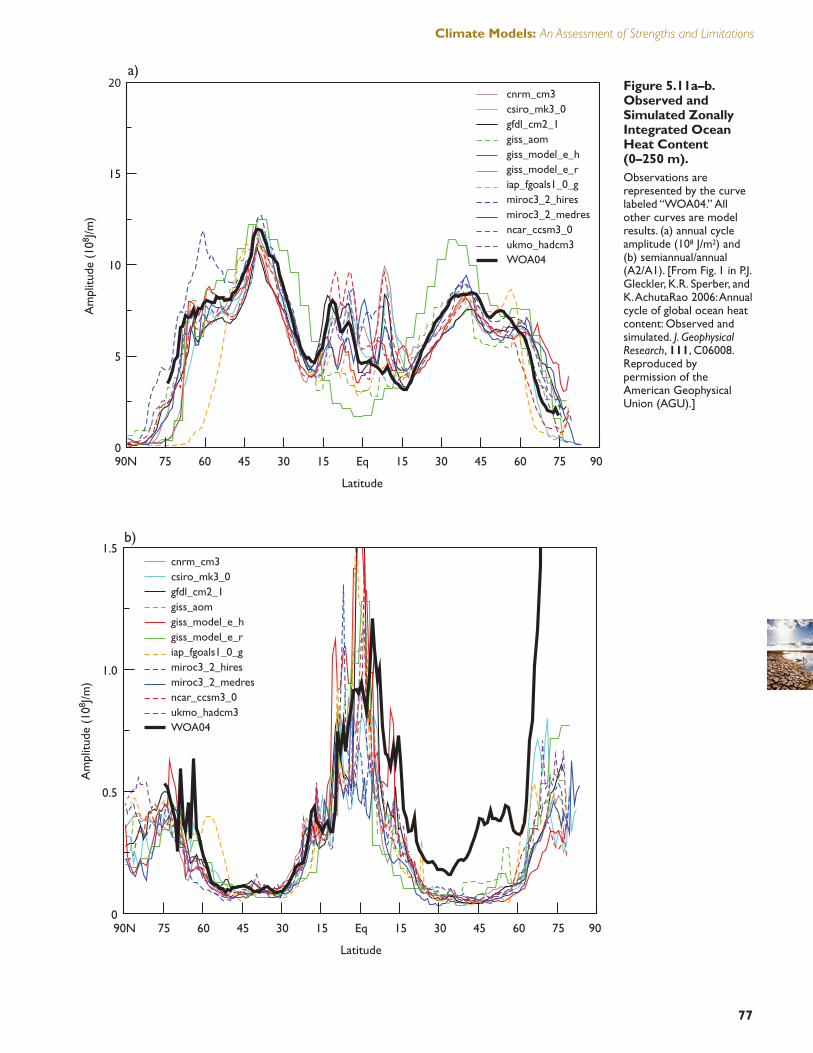
77


20

15

10

5

0

Am

plitu

de (

108 J

/m)

Latitude

90N 75 60 45 30 15 15Eq 30 45 60 75 90

cnrm_cm3csiro_mk3_0gfdl_cm2_1giss_aomgiss_model_e_hgiss_model_e_riap_fgoals1_0_gmiroc3_2_hiresmiroc3_2_medresncar_ccsm3_0ukmo_hadcm3WOA04

a)

Latitude

90N 75 60 45 30 15 15Eq 30 45 60 75 90S

cnrm_cm3csiro_mk3_0gfdl_cm2_1giss_aomgiss_model_e_hgiss_model_e_riap_fgoals1_0_gmiroc3_2_hiresmiroc3_2_medresncar_ccsm3_0ukmo_hadcm3WOA04

1.5

1.0

0.5

0

Am

plitu

de (

108 J

/m)

b)

Figure 5.11a–b.Observed andSimulated ZonallyIntegrated OceanHeat Content (0–250 m).Observations arerepresented by the curvelabeled “WOA04.” Allother curves are modelresults. (a) annual cycleamplitude (108 J/m2) and(b) semiannual/annual(A2/A1). [From Fig. 1 in P.J.Gleckler, K.R. Sperber, andK. AchutaRao 2006: Annualcycle of global ocean heatcontent: Observed andsimulated. J. GeophysicalResearch, 111, C06008.Reproduced bypermission of theAmerican GeophysicalUnion (AGU).]

78


a) Global d) Tropics (20S-20N)

b) Northern Hemisphere e) Southern Ocean

c) Southern Hemisphere

Hea

t C

onte

nt (

10**

22J)

f) Arctic Ocean

Month Month

J F M A M J J A S O N D J F M A M J J A S O N D



543210

–1–2–3–4–5

121086420

–2–4–6–8

–10–12

14121086420

–2–4–6–8

–10–12–14

2

1

0

–1

–2

2

1

0

–1

–2

2

1

0

–1

–2

cnrm_cm3csiro_mk3_0gfdl_cm2_1giss_aomgiss_model_e_hgiss_model_e_riap_fgoals1_0_gmiroc3_2_hiresmiroc3_2_medresncar_ccsm3_0ukmo_hadcm3WOA01WOA04

Figure 5.12a–f. Annual Cycle of Observed and Simulated Basin Average Global Ocean Heat Content (0–250 m). Observations are represented by the curves labeled “WOA01” and “WOA04.” Units are 1022 J. Arctic Ocean is defined as north of 60°N,and Southern Ocean is south of 60°S. [From Fig. 3 in P.J. Gleckler, K.R. Sperber, and K. AchutaRao 2006: Annual cycle of global ocean heatcontent: Observed and simulated. J. Geophysical Research, 111, C06008. Reproduced by permission of the American Geophysical Union(AGU).]

79


5.2.5 Global Mean Sea-Level Rise

Two separate physical processes contribute tosea-level rising: (1) ocean thermal expansionfrom an increase in ocean heat uptake (stericcomponent) and (2) addition of freshwater fromprecipitation, continental ice melt, and riverrunoff (eustatic component). Various oceanmodels handle freshwater fluxes in differentways. With the addition of a free surface in thecurrent generation of ocean models, freshwaterflux into oceans can be included directly(Griffies et al. 2001). The freshwater contribu-tion is computed in quantities estimated by theclimate model’s atmosphere and ice-sheet com-ponents (e.g., Church, White, and Arblaster2005; Gregory, Lowe, and Tett 2006). In gen-eral, state-of-the-art climate models underesti-mate the combined global mean sea-level riseas compared to tide gauge and satellite altime-ter estimates, while the rise for each separatecomponent is within the observed values’ un-certainty. The reason for this is an open researchquestion and may relate either to observationalsampling or to incorrectly accounting for all eu-static contributions. The steric component toglobal mean sea-level rise is estimated at 0.40 ±0.05 mm/yr from observations (Antonov, Levi-tus, and Boyer 2005). Models simulate a similarbut somewhat smaller rise (Gregory, Lowe, andTett 2006; Meehl et al. 2005). Significant dif-ferences also occur in the magnitudes ofdecadal variability between observed and simu-lated sea level. Progress is being made, however,over the previous generation of climate models.When atmospheric effects from volcanic erup-tions are included, for example, current-gener-ation ocean models capture the volcanoes’observed impact (a decrease in the global meansea level). Figure 5.13 from Church, White, andArblaster (2005) gives an example of a fewmodels and their detrended estimate of the his-toric global mean sea level. It shows the influ-ence of including additional atmosphericforcing agents in changing the ocean’s stericheight.

5.3 EXTREME EVENTS

Flood-producing precipitation, drought, heatwaves, and cold waves have severe impacts onNorth America. Flooding resulted in averageannual losses of $3.7 billion between 1983 and

2003 (www.flooddamagedata.org). Losses fromthe 1988 drought were estimated at $40 billionand the 2002 drought at $11 billion. Heat wavesin 1995 resulted in 739 additional deaths inChicago alone (Whitman et al. 1997). A largecomponent of overall climate change impactsprobably will arise from changes in the inten-sity and frequency of extreme events.

Modeling of extreme events poses special chal-lenges since they are, by definition, rare. Al-though the intensity and frequency of extremeevents are modulated by ocean and land surfacestate and by trends in the mean climate state, in-ternal atmospheric variability plays a very largerole, and the most extreme events arise fromchance confluence of unlikely conditions. Thevery rarity of extreme events makes statisticalevaluation of model performance less robustthan for mean climate. For example, in evaluat-ing a model’s ability to simulate heat waves asintense as that in 1995, only a few episodes inthe entire 20th Century approach or exceed thatintensity (Kunkel et al. 1996). For such rareevents, estimates of the real risk are highly un-certain, varying from once every 30 years toonce every 100 years or more. Thus, a modelthat simulates these occurrences at a frequencyof once every 30 years may be performing ade-quately, but its performance cannot be distin-guished from that of the model that simulates afrequency of once every 100 years.

Although it might be expected that a change inmean climate conditions will apply equally tochanges in extremes, this is not necessarily thecase. Using as an example the 50-state record-low temperatures, the decade with the largestnumber of records is the 1930s, yet winters dur-ing that decade averaged third warmest since1890; in fact, no significant correlation isshown between the number of records and U.S.wintertime temperature (Vavrus et al. 2006).Thus, the severest cold air outbreaks in the pastdo not necessarily coincide with cold winters.Another examination of model data showed thatfuture changes in extreme temperatures differfrom changes in mean temperature in many re-gions (Hegerl et al. 2004). This means that cli-mate model output must be analyzed explicitlyfor extremes by examining daily (or even finer–resolution) data, a resource-intensive effort.

80


1960 1965 1970 1975 1980 1985 1990 1995 2000−8x10 22

−4x10 22

0

4x10 22

8x10 22

Heat content Model (PCM)LevitusIshii

Hea

t co

nten

t (J)

(a)

Agung El ChichonPinatubo

1960 1965 1970 1975 1980 1985 1990 1995 2000−10

−5

0

5

10GMS L Model (PCM)Levitus

Ishii

GM

SL (

mm

)

(b)


1960 1965 1970 1975 1980 1985 1990 1995 2000−10

−5

0

5

10MIROC3.2(hires)MIROC3.2(medres)

GISS−ERPCM

GMS L


(c)

GM

SL (

mm

)

Figure 5.13. Observed and Modeled Global Ocean Heat Content (GOHC) and Global Mean Sea Level (GMSL)for 1960 to 2000. The response to volcanic forcing, as indicated by differences between pairs of PCM simulations for GOHC (a) and GMSL (b) is shown forthe ensemble mean (bold line) and the three ensemble members (light lines). Observational estimates of GOHC and GMSL are shown bythe black and blue bold lines. For a and b, all results are for the upper 300 m only and have been detrended over the period 1960 to 2000.For c, the ensemble mean (full-depth) GMSL for GISS-ER, MIROC3.2(hires), MIROC3.2(medres), and PCM models (after subtracting aquadratic) are shown. [From Fig. 2 in J.A. Church, N.J. White, and M. Arblaster 2005: Significant decadal-scale impact volcanic eruptions onsea level and ocean heat content. Nature, 438(7064), 74–77. Used with permission from Nature Publishing Group.]

81


Evaluation of model performance with respectto extremes is hampered by incomplete data onhistorical frequency and severity of extremes.Frich et al. (2002) analyzed ten indicators of cli-mate extremes and presented global results.However, many areas were missing due to lackof suitable station data, particularly in the trop-ics. Using some of these indices for compar-isons between models and observations hasbecome common. Another challenge for modelevaluation is the spatially averaged nature ofmodel data, representing an entire grid cell,while station data represent point observations.For some comparisons, averaging station dataover areas representing a grid cell is necessary.

Several approaches are used to evaluate modelperformance for simulation of extremes. Oneapproach examines whether a model reproducesthe magnitude of extremes. For example, a dailyrainfall amount of 100 mm or more is expectedto occur about once every year in Miami, every6 years in New York City, every 13 years inChicago, and every 200 years in Phoenix. Auseful metric would be the extent to which amodel is able to reproduce absolute magnitudesand spatial variations of such extremes. A sec-ond approach examines whether a model repro-duces observed trends in extremes. Perhaps themost prominent observed global trend is an in-crease in the frequency of heavy precipitation,particularly during the last 20 to 30 years of the20th Century. This trend is significant at the 95%confidence level for the period 1979 to 2003and at the 99% confidence level for the period1951 to 2003 (Trenberth et al. 2007). Anothernotable observed trend is an increase in thelength of the frost-free season.

In some key respects, model simulation of tem-perature extremes probably is less challengingthan simulating precipitation extremes, in largepart due to the scales of these phenomena. Thetypical heat wave or cold wave covers a rela-tively large region, on the order of several hun-dred miles or more or a number of grid cells ina modern climate model. By contrast, heavyprecipitation can be much more localized, oftenextending over regions of much less than 150km, or less than the size of a grid cell. Thus, themodern climate model can simulate directly themajor processes causing temperature extremeswhile heavy precipitation is sensitive to para-

meterization of subgrid-scale processes, partic-ularly convection (Chapter 2; Emori and Brown2005; Iorio et al. 2004).

5.3.1 DROUGHTS AND EXCESSIVE RAINFALL

LEADING TO FLOODS

Recent analysis indicates a globally averagedtrend toward greater areal coverage of droughtsince 1972 (Dai et al. 2004). A simulation bythe HadCM3 model reproduces this dry trend(Burke, Brown, and Christidis 2006) only if an-thropogenic forcing is included. A control sim-ulation indicates that the observed drying trendis outside the range of natural variability. Themodel, however, does not always correctly sim-ulate the regional distributions of areas of in-creasing wetness and dryness. The relationshipbetween droughts and variability was coveredabove in Section 5.2.2.3 Monsoons.

Several different measures of excessive rainfallhave been used in analyses of model simula-tions. A common one is the annual maximum5-day precipitation amount, one of the Frich etal. (2002) indices. This has been analyzed inseveral recent studies (Kiktev et al. 2003;Hegerl et al. 2004; Tebaldi et al. 2006). Otheranalyses have examined thresholds of daily pre-cipitation, either absolute (e.g., 50 mm/day inDai 2006) or percentile (e.g., 4th-largest precip-itation event equivalent to 99th percentile of 365daily values as in Emori et al. 2005). Recentstudies of model simulations produced forCMIP3 provide information on the performanceof the latest model generation.

Models generally tend to underestimate veryheavy precipitation. This is shown in a compar-ison between satellite (TRMM) estimates ofdaily precipitation and model-simulated valueswithin the 50°S–50°N latitude belt (Dai 2006).TRMM observations derive 7% of total precip-itation from very heavy rainfall of 50 mm ormore per day, in contrast to only 0 to 2% for themodels. For the frequency of very heavy pre-cipitation of 50 mm or more per day, TRMMdata show a frequency of 0.35% (about onceevery 300 days), whereas it is 0.02 to 0.11%(once every 900 to 5000 days) for the models. Aglobal analysis of model simulations showedthat models produced too little precipitation inevents exceeding 10 mm/day (Sun et al. 2006).Examining how many days it takes to accumu-

82


late two-thirds of annual precipitation, modelsgenerally show too many days compared to ob-servations over North America, although a fewmodels are close to reality. In contrast to thegeneral finding of a tendency toward underesti-mation, a study (Hegerl et al. 2004) of two mod-els indicates generally good agreement withobserved annual maximum 5-day precipitationamounts over North America for HadCM3 andeven somewhat of an overestimation forCGCM2.

This model tendency to produce rainfall eventsless intense than observed appears to be due inpart to global models’ low spatial resolution.Experiments with individual models show thatincreasing resolution improves the simulationof heavy events. For example, the fourth-largestprecipitation event in a model simulation with aresolution of about 300 km averaged 40 mmover the conterminous United States, comparedto an observed value of about 80 mm. When theresolution was increased to 75 km and 50 km,the fourth-largest event was still smaller thanobserved but by a much smaller amount (Iorioet al. 2004). A second important factor is the pa-rameterization of convection. Thunderstormsare responsible for many intense events, buttheir scale is smaller than the size of modelgrids and thus must be indirectly represented inmodels (Chapter 2). One experiment showedthat changes to this representation improvemodel performance and, when combined withhigh resolution of about 1.1° latitude, can pro-duce quite-accurate simulations of the fourth-largest precipitation event on a globallyaveraged basis (Emori et al. 2005). Another ex-periment found that the use of a cloud-resolv-ing model imbedded in a global modeleliminated underestimation of heavy events(Iorio et al. 2004). A cloud-resolving modeleliminates the need for convection parameteri-zation but is very expensive to run. These sets ofexperiments indicate that the problem of heavy-event underestimation may be reduced signifi-cantly in future as increases in computer powerallow simulations at higher spatial resolutionand perhaps eventually the use of cloud-resolv-ing models.

Improved model performance at higher spatialresolutions provides motivation for use of re-gional climate models when only a limited area,

such as North America, is of interest. Thesemodels have spatial resolution sufficient to re-solve major mountain chains, and some thusdisplay considerable skill in areas where topog-raphy plays a major role in spatial patterns. Forexample, they are able to reproduce rather wellthe spatial distribution of the magnitude or ex-tent of precipitation in the 95th percentile (Leungand Qian 2003), frequency of days with morethan 50 mm and 100 mm (Kim and Lee 2003),frequency of days over 25 mm (Bell, Sloan, andSnyder 2004), and annual maximum daily pre-cipitation amount (Bell, Sloan, and Snyder2004) over the western United States. Kunkel etal. (2002) found that an RCM’s simulation ofextreme-event magnitude over the United Statesvaried spatially and depended on event duration.There was a tendency for overestimation inwestern United States and good agreement orunderestimation in central and eastern UnitedStates.

Most studies of observed precipitation extremessuggest that they have increased in frequencyand intensity during the latter half of the 20th

Century. A study by Tebaldi et al. (2006) indi-cates that models generally simulate a trend to-ward a world characterized by intensifiedprecipitation, with a greater frequency of heavy-precipitation and high-quantile events, althoughwith substantial geographical variability. This isin agreement with observations. Wang and Lau(2006) find that CGCMs simulate an increasingtrend in heavy rain over the tropical ocean.

5.3.2 Heat and Cold Waves

Analyses of simulations for IPCC AR4 by sevenclimate models indicate that they reproduce theprimary features of cold air outbreaks (CAOs),with respect to location and magnitude (Vavruset al. 2006). In the analyses, a CAO is anepisode of at least 2 days duration during whichthe daily mean winter (December-January-February) surface temperature at a gridpoint istwo standard deviations below the gridpoint’swinter mean temperature. Maximum frequen-cies of about four CAO days per winter are sim-ulated over western North America and Europe,while minimal occurrences of less than one dayper winter exist over the Arctic, northern Africa,and parts of the North Pacific. GCMs generallyare accurate in their simulation of primary fea-

83


tures, with high pattern correlation to observa-tions and maximum number of days meetingCAO criteria around 4 per winter. One favoredregion for CAOs is in western North America,extending from southern Alaska into the upperMidwest. Here, models simulate a frequency ofabout 4 CAO days per year, in general agree-ment with the observed values of 3 to 4 days.Models underestimate frequency in the south-eastern United States (mean simulated valuesrange from 0.5 to 2 days vs 2 to 2.5 days in ob-servations). This regional bias occurs in allmodels and reflects the inability of GCMs topenetrate Arctic air masses far enough south-eastward over North America.

CMIP3 model simulations show a positive trendfor growing season, heat waves, and warmnights and a negative trend for frost days anddaily temperature range (maximum minus min-imum) (Tebaldi et al. 2006). The simulations in-dicate that this is in general agreement withobservations, except that there is no observedtrend in heat waves. The modeled spatial pat-terns generally have larger positive trends inwestern North America than in eastern sections.For the United States, this is in qualitativeagreement with observations showing that de-creases in frost-free season and frost days arelargest in the western United States (Kunkel etal. 2004; Easterling 2002).

Analysis of individual models provides a moredetailed picture of model performance. In a sim-ulation from PCM (Meehl, Tebaldi, and Nychka2004), the largest trends for decreasing frostdays occur in the western and southwesternUnited States (values greater than –2 days perdecade). Trends near zero in the upper Midwestand northeastern United States show goodagreement with observations. The biggest dis-crepancy between model and observations isover parts of the southeastern United States,where the model shows trends for decreasingfrost days and observations show slight in-creases. This is thought to be a partial conse-quence of two large El Niño events inobservations during this time period (1982–1983 and 1997–1998) when anomalously cooland wet conditions occurred over the southeast-ern United States and contributed to slight in-creases of frost days. The model’s ensemblemean averages out effects from individual El

Niño events, and thus frost-day trends reflect amore general response to forcings that occurredduring the latter part of the 20th Century. Ananalysis of short-duration heat waves simulatedby PCM (Meehl and Tebaldi 2004) indicatesgood agreement with observed heat waves forNorth America. In that study, heat waves weredefined by daily minimum temperature. Themost intense events occurred in the southeasternUnited States for both model simulation and ob-servations. The overall spatial pattern of heat-wave intensity in the model matched closelywith the observed pattern. In a four-member en-semble of simulations from HadCM3 (Chris-tidis et al. 2005), the model showed a ratheruniform pattern of increases in the warmestnight for 1950 to 1999. Observations also showa global mean increase, but with considerableregional variations. In North America, observedtrends in the warmest night vary from negativein the south-central sections to strongly positivein Alaska and western Canada, compared to arather uniform pattern in the model. However,this discrepancy might be expected, since theobservations probably reflect a strong imprintof internal climate variability that is reduced byensemble averaging of the model simulations.

Analysis of the magnitude of temperature ex-tremes for California in a regional climatemodel simulation (Bell, Sloan, and Snyder2004) shows mixed results. The hottest maxi-mum in the model is 4°C less than observations,while the coldest minimum is 2.3°C warmer.The number of days >32°C is 44 in the modelcompared to an observed value of 71. Thiscould result from the lower diurnal temperaturerange in the model (15.4°C observed vs 9.7°Csimulated). While these results are better thanthe driving GCM, RCM results are still some-what deficient, perhaps reflecting the study re-gion’s very complex topography.

Models display some capability to simulate ex-treme temperature and precipitation events, butthere are differences from observed character-istics. Models typically produce global in-creases in extreme precipitation and severedrought and decreases in extreme minimumtemperatures and frost days, in general agree-ment with observations. Models have a general,though not universal, tendency to underestimatethe magnitude of heavy precipitation events.

84


Regional-trend features are not always captured.Since the causes of observed regional-trendvariations are not known in general and suchtrends could be due in part to the climate sys-tem’s stochastic variability, assessing the sig-nificance of these discrepancies is difficult.


Future Model Development

CH

APT

ER6

85

Climate models are evolving toward greater comprehensiveness, incorporating such aspects of the

chemical and biological environment as active vegetation on land and oceanic biogeochemistry that

affect and are affected by the physical climate. Climate models are simultaneously evolving to-

ward finer spatial resolution.

Improvements in climate simulations as resolution increases can be both incremental and funda-

mental. Incremental improvements are expected in treatment of the atmosphere due to better

simulation of atmospheric fronts, interactions among extratropical storms and sharp topographic

features, and, especially, tropical storms. In the ocean, finer resolution incrementally improves the

simulation of narrow boundary currents and the circulation in relatively small basins, such as the

Labrador Sea, that play key roles in oceanic circulation.

More fundamental changes also happen in both the atmosphere and the ocean as resolution im-

proves. In the ocean a key transition occurs at grid scales of tens of kilometers, at which point

mesoscale eddies (see Chapter 2) begin to be explicitly resolved. In the atmosphere, a funda-

mental transition takes place when the grid scale drops to a few kilometers, where direct simu-

lation of dominant deep convective circulations begins to be feasible and the model’s dependence

on uncertain subgrid-scale parameterization of deep moist convection diminishes.

In the following, we discuss these more funda-mental oceanic and atmospheric transitions andthen describe some examples of increased com-prehensiveness in climate modeling (see alsoChapter 2 for glacial modeling, another impor-tant future development).

The climate modeling enterprise is evolvingalong additional paths (apart from evolution ofthe models themselves) that are not discussedhere. One path is the creation of large ensem-bles of model simulations by varying uncertain

physical parameters so as to better estimate theassociated uncertainties [quantifying uncer-tainty in model predictions (called QUMP);Murphy et al. 2004; climateprediction.net]. Oth-ers include the movement toward initializing cli-mate models with estimates of observedclimatic states, particularly the observedoceanic state, so as to optimize the realism ofdecadal forecasts, which marks an evolution to-ward the merging of seasonal-interannual anddecadal forecasting (Troccoli and Palmer 2007).

Chapter 6 - Future Model DevelopmentThe U.S. Climate Change Science Program

86

6.1 HIGH-RESOLUTION MODELS

6.1.1 Mesoscale Eddy-ResolvingOcean Models

The distinction between laminar and turbulentflow in the ocean is fundamental. Simulationsof the more realistic turbulent regime promiseto substantially raise the level of realism inoceanic climate simulations. For example, Fig.6.1 shows two simulations of the SouthernOcean by an ocean model developed at the Geo-physical Fluid Dynamics Laboratory (GFDL)(Hallberg and Gnanadesikan 2006). The fieldshown is an instantaneous snapshot of the sur-face current speed. Resolution of the model onthe left is about 1° latitude. The result is a rela-tively laminar (nonturbulent) flow with a gen-tly meandering circumpolar current. The figureon the right is obtained by reducing the grid size

to 1/6 of a degree. A much more turbulent flowis simulated by the model with abundant vortexgeneration. This model is beginning to resolvethe spectrum of mesoscale eddies that populatethe Southern Ocean and many other oceanic re-gions. As discussed in Chapter 2, the effects onocean circulation of mesoscale eddy-inducedmixing are parameterized in current ocean mod-els, which can be thought of as essentially lam-inar.

While progress has been made in recent years,explicit simulation of these eddies undoubtedlyis more reliable than mixing parameterizations.In the Southern Ocean, eddies are thought tocontrol the circumpolar current’s response towind changes (Hallberg and Gnanadesikam2006) and the way carbon dioxide is taken upby the Southern Ocean.

Figure 6.1. Surface-Current Speed in Two Simulations of the Southern Ocean in Low-and High-Resolution Ocean Models. [From Fig. 6 in R. Hallberg and A. Gnanadesikam 2006: The role of eddies in determining the structure andresponse of the wind-driven Southern Hemisphere overturning: Results from the modeling eddies in theSouthern Ocean (MESO) project. J. Physical Oceanography, 36, 2232–2252. Reproduced by permission ofthe American Meteorological Society (AMS).]

Global mesoscale eddy-resolving ocean modelsare beginning to be examined in various mod-eling centers in the United States and around theworld, even though exploiting such models willrequire substantial increases in computationalresources. Challenges that may arise when thesemodels are integrated for long time periods in-clude maintaining realistically small amounts ofmixing across constant-density surfaces in themore turbulent flows to avoid distortion ofmuch slower thermohaline circulations.

As noted in Chapter 5, models provide esti-mates of the climate system’s centennial-scalevariability that underlies attribution studies ofclimatic trends. Seeing if eddy-resolvingOGCMs increase the variability level on longtime scales in climate models will be of greatinterest.

6.1.2 Cloud-Resolved AtmosphericModels

As atmospheric models attain higher resolutionand more detailed representation of physicalprocesses, short-range weather prediction andlonger-range climate prediction become moresynergistic (Phillips et al. 2004). This is partic-ularly evident in “cloud-resolving models”(CRMs) with spatial resolutions of less than afew kilometers. CRMs can explicitly simulateatmospheric systems that exist on scales muchsmaller than the grid resolution of conventionalatmospheric general circulation models(AGCMs) (Randall et al. 2003; Khairoutdinov,Randall, and DeMott 2005). These systems in-clude mesoscale organizations in squall lines,deep updrafts and downdrafts, and cirrus anvils.CRMs also allow calculation of cloud proper-ties and amounts based on more realistic small-scale structure in the flow field. The desiredresult is not only better simulations of regionalclimates, especially in the tropics, but also morereliable estimates of cloud feedbacks and cli-mate sensitivity.

CRMs are variations of models designed formesoscale storm and cumulus convection sim-ulations. At CRM grid scales, hydrostatic bal-ance is no longer universally valid. CRMs aretherefore formulated with nonhydrostatic equa-tions in which vertical accelerations are calcu-lated explicitly (Tripoli 1992).

Like AGCMs, CRMs must employ empiricalparameterizations to calculate the impact ofsubgrid scale processes, but CRMs explicitlyrepresent a larger portion of the size spectrumof meteorological systems, so the parameteri-zations’ impact on large-scale circulation andclimate may be less severe. Most important, cu-mulus parameterizations for deep tropical con-vection are not needed in CRMs. CRMs canaccommodate more realistic microphysicalprocesses, including those by which aerosolsnucleate cloud drops, allowing more convinc-ing treatment of aerosol and cloud interactionsinvolved in indirect aerosol radiative forcing.

However, shallow nonprecipitating convection(which produces fair-weather cumulus clouds)is dominated by flows on scales less than 1 kmand will probably still require subgrid-scale pa-rameterization in foreseeable global CRMs.Cloud feedbacks in regions of shallow convec-tion are an important source of disparity in cli-mate sensitivity in CMIP3 models (Bony et al.2006). Furthermore, most cloud microphysicalprocesses take place on CRM subgrid scalesand so must be parameterized. Thus, uncertaintyin cloud feedbacks will not disappear whenglobal CRMs begin to play a role in climate as-sessments, but modelers hope that uncertaintywill be reduced substantially.

Global models with CRM resolution have beenattempted to date only at the Japanese EarthSimulator, but, with continued increase in com-puter power, global CRMs are expected to be-come centrally important in climate (as well asweather) research. Nevertheless, as noted above,major uncertainties in cloud microphysics willremain, especially in the prediction of ice-parti-cle concentrations, fall speed of cloud particles,hydrometeorological spectra evolution, and en-trainment rates into convective plumes (Cotton2003). At CRM resolutions, more sophisticatedalgorithms of radiative-transfer calculation thanthose in current GCMs may be required becausethe plane parallel assumption for convergence ofradiant energy may not be valid. Validation ofCRMs probably will continue to take place in re-gional models and short-range forecasts, fol-lowed by their incorporation into global models.

Several observational programs such as theDOE Atmospheric Radiation Measurement


87

88

The U.S. Climate Change Science Program Chapter 6 - Future Model Development

(ARM) Program have collected data essential toevaluate CRMs (M.H. Zhang et al. 2001; Tao etal. 2004). Results from such programs will facil-itate improvement of CRM subgrid-scalephysics. Extensive parameter-sensitivity testswith global models will still be needed to reduceuncertainties in microphysics and the treatmentof shallow convection for climate sensitivity andregional climate-change simulation.

6.2 BIOGEOCHEMISTRY ANDCLIMATE MODELS

6.2.1 Carbon Cycle

The physical climate system and biogeochemi-cal processes are tightly coupled. Changes inclimate affect the exchange of atmospheric CO2

between land surface and ocean, and changes inCO2 fluxes affect Earth’s radiative forcing andthus the physical climate system. Some recentlydeveloped atmosphere-ocean general circula-tion models (AOGCMs) include the carboncycle and have confirmed the potential forstrong feedback between it and global climate(Cox et al. 2000; Friedlingstein et al. 2001;Govindasamy et al. 2005). The next generation ofAOGCMs may include the carbon cycle as well asinteractive atmospheric aerosols and chemistry.Models that include the carbon cycle are able topredict time-evolving atmospheric CO2 concen-trations using, as input, anthropogenic emissionsrather than assumed concentrations.

Simulation of the global carbon cycle must ac-count for the processes shown in Fig. 6.2. As thefigure shows, the present-day global carbon cycleis not in equilibrium because of fossil-fuel burn-ing and other anthropogenic carbon emissions.These carbon sources must, of course, be in-cluded in models of climate change. Such a cal-culation is not easy because human-inducedchanges to the carbon cycle are small compared tolarge natural fluxes, as shown in the figure. In ad-dition, although the globally and annually aver-aged carbon reservoirs and fluxes shown in thefigure are consistent with estimates from a varietyof sources, substantial uncertainties are attachedto the numbers (e.g., often a factor >2 uncertaintyfor fluxes; see Prentice et al. 2001). Additionaluncertainty applies to regional, seasonal, and in-terannual variations in the carbon cycle.

Feedbacks between the physical climate systemand the carbon cycle are represented plausiblybut with substantial differences in variousAOGCM carbon-cycle models. Cox et al.(2000) obtained a very large positive feedback,with global warming reducing the fraction ofanthropogenic carbon absorbed by the bios-phere, thus boosting the model’s simulated at-mospheric CO2. Friedlingstein et al. (2001)obtained much weaker feedback. Thompson etal. (2004) demonstrated that making differentassumptions about the land biosphere within asingle model gave markedly different feedbackvalues. Using the same model, Govindasamy etal. (2005) noted a positive correlation betweenthe magnitude of carbon-cycle feedback and thesensitivity of the physical climate system.

A recent study examined carbon-cycle feed-backs in 11 coupled AOGCM carbon-cyclemodels using the same forcing (Friedlingsteinet al. 2006). The models unanimously agreedthat global warming will reduce the fraction ofanthropogenic carbon absorbed by the bios-phere—a positive feedback—but the magnitudeof this feedback varied widely among models(Fig. 6.3). When models included an interactivecarbon cycle, predictions of the additionalglobal warming due to carbon-cycle feedbackranged between 0.1 and 1.5°C. Eight models at-tributed most of the feedback to the land bios-phere, while three attributed it to the ocean.

These results demonstrate the large sensitivityof climate model output to assumptions aboutcarbon-cycle processes. Future carbon-cyclemodels, coupled to physical climate models andconstrained by new global remote-sensingdatasets and in situ measurements, may allowmore definitive projection of CO2 concentra-tions in the atmosphere for given emission sce-narios. CCSP SAP 2.2 contains moreinformation on the carbon cycle and climatechange (CCSP 2007).

6.2.2 Other Biogeochemical Issues

Methane (CH4) is a potent greenhouse gaswhose atmospheric concentration is controlledby its emission rate and the atmosphere’s oxida-tive capacity (especially hydroxyl radical con-centration). Methane concentrations are nowmuch higher than in preindustrial times but have

89


not increased in the past decade, for reasons thatcontinue to be debated. Whether or not this trendcarries into the future has substantial implicationsfor radiative forcing. To resolve this question,AOGCMs would need to include atmosphericchemistry models incorporating a number of dif-ferent trace gases and reaction rates.

Another emerging issue is the interactive evo-lution of climate with the storage of water and

carbon by plants. To address this process, dy-namic vegetation models (in which plant growthis calculated rather than specified a priori) areunder development at modeling centers in theUnited States and elsewhere. This inclusion of awider range of processes poses challenges [e.g.,it amplifies errors in rainfall prediction (Bonanand Levis 2006)]. In addition, ecosystems fer-tilized with CO2 are limited by the availabilityof nutrients such as nitrogen and phosphorous

Figure 6.2. GlobalCarbon Cycle from the Point of View ofExisting PhysicalClimate SystemModels (CoupledAOGCMs). The four boxes representatmosphere, land surface,ocean, and sea ice—majorcomponents of AOGCMs.Earth system models willevolve from AOGCMs byincorporating relevantbiogeochemical cycles intothe four-box framework(with sea ice not acting as acarbon reservoir). Numbersshown are average values forthe 1990s. Small (≤1PgC/year) fluxes such asthose involving methane arenot shown, except for burialof 0.2 PgC/year in ocean-bottom sediments, assuminga 50-50 split between plantand microbial respiration.

Global Carbon Cycle as Seen by an AOGCM

surface dissolvedinorganic

Ocean

Atmosphere

Land surface

Sea ice

760

920

3

37000

150

marine biota

deep ocean

ocean sediments

vegetationand soils

2300

3500fossil fuels

123photosynthesis

GPP

NPP}92

0.2

Circled numbers =

storage in gigatonnes (or petagrams) carbon

Other numbers =

fluxes in gigatonnes carbon/year

11

92 10192 101deep-surfacedeep-surface

oceanoceanexchangeexchange

39 remineralization39 remineralizationphotosynthesis 50photosynthesis 50

6fossil-fuel burningfossil-fuel burning

and cement productionand cement production

6060microbialmicrobial

respirationrespiration

6060plantplantresp.resp.

2land-coverland-cover

changechange

9191ocean-atmocean-atmexchangeexchange

92 101deep-surface

oceanexchange

39 remineralizationphotosynthesis 50

6fossil-fuel burning

and cement production

60microbial

respiration

60plantresp.

2land-cover

change

91ocean-atmexchange

rivers

1

Figure 6.3. Time Seriesof Atmospheric CO2

from 11 DifferentAOGCM Carbon-Cycle Models. [From Fig. 1(a) of P.Friedlingstein et al. 2006:Climate-carbon cyclefeedback analysis: Resultsfrom the C4MIP modelintercomparison. J. Climate,19, 3337–3353. Reproducedby permission of theAmerican MeteorologicalSociety (AMS).]

Atm

osph

eric

CO

2 (p

pm)

1000

900

800

700

600

500

400

300

1850 1900 1950 2000 2050 2100Year

90

The U.S. Climate Change Science Program Chapter 6 - Future Model Development

that are important to the carbon cycle (Field,Jackson, and Mooney 1995; Schimel 1998;Nadelhoffer et al. 1999; Shaw et al. 2002; Hun-gate et al. 2003). Future climate-carbon modelsprobably will need to include these nutrients.The few models that do so now show less plantgrowth in response to increasing atmosphericCO2 (Cramer et al. 2001; Oren et al. 2001;Nowak, Ellsworth, and Smith 2004). Incorpo-ration of other known limiting factors such asacclimation of soil microbiology to higher tem-peratures (Kirschbaum 2000; Tjoelker, Oleksyn,and Reich 2001) will be important in develop-ing comprehensive Earth system models.Aerosol modeling also will be a central elementin future models (this subject will be covered byCCSP SAP 2.3, whose estimated publicationdate is June 2008).

Often, climate-carbon simulations include nat-ural ecosystems but do not include the effectsof human land-cover and land-managementchanges (e.g., deforestation and reforestation).Land-cover change often is accounted for sim-ply by prescribing estimates for the historicalperiod (e.g., Houghton 2003) and for future sce-narios from the IPCC Special Report on Emis-sions Scenarios (IPCC 2000). These estimatesdo not include practices such as crop irrigationand fertilization. Many models with “dynamicvegetation” do not actually simulate crops; theyonly allow natural vegetation to grow. Defor-estation, land cultivation, and related human ac-tivities probably will be included in at leastsome future AOGCMs, enabling more completeassessment of total anthropogenic effects on theglobal climate and environment (Ramankutty etal. 2002; Root and Schneider 1993).

6.2.3 Ocean Biogeochemistry

Climate change impacts on the marine environ-ment—including changes in the ocean’s biotaand carbon content due to modified ocean tem-perature, salinity, and circulation patterns—must be accounted for, along with terrestrialbiogeochemistry, in a complete Earth systemmodel. Implementation of ocean biogeochem-istry processes into AOGCMs is under way to improve simulation of the ocean carbon cycle under various scenarios [e.g., “CCSMBiogeochemistry Working Group Meeting Report,” March 2006 (www.ccsm.ucar.edu/

working_groups/Biogeo/reports/060328_BGCWGrpt.pdf); GFDL’s Earth system model(gfdl.noaa.gov/~jpd/ esmdt.html); Doney et al.2004]. One issue receiving particular attentionin recent years is that ocean productivity maybe increased through iron fertilization via dustparticles, potentially reducing atmospheric CO2

(Martin 1991). This effect is being assessed byboth observational programs (e.g., Bishop,Davis, and Sherman 2002) and climate-carbonmodels (Jickells et al. 2005).

An important challenge to these efforts is thecomplexity of ocean ecosystems. Adding to thiscomplexity are organisms that fix nitrogen anddenitrify, calcify, or silicify; accounting for eachadds parameterizations and variables to the sys-tem (Hood et al. 2006). Biological models needto be sufficiently complex to capture the ob-served variability on various time scales, sincethis variability provides essential tests for themodels. As in many aspects of climate model-ing, however, complexity that outgrows the abil-ity to constrain models with available datashould be avoided (Hood et al. 2006).

Modeling groups have undertaken systematiccomparison of different models in the OceanCarbon Cycle Model Intercomparison Project(OCMIP) under the auspices of the Interna-tional Geosphere-Biosphere Programme.OCMIP’s most recent phase involved 13groups—including several from the UnitedStates—implementing a common biologicalmodel in their different OGCMs (Najjar et al.2007). The common biological model includesfive prognostic variables: inorganic phosphate(PO4

2–), dissolved organic phosphorus (DOP),dissolved oxygen (O2), dissolved inorganic car-bon (CO2 + HCO3

– + CO32–), and total alkalin-

ity (the system’s acid- and base-bufferingcapacity). Model intercomparison revealed sig-nificant differences in simulated biogeochemi-cal fluxes and reservoirs. A biogeochemistrymodel’s realism was found to be tied closely tothe dynamics of the simulation’s ocean circula-tion. Just as for land vegetation modeling, a se-rious challenge to climate models is presentedby the quality of the physical climate simulationrequired for realistic biogeochemical modeling.


Example Applications of Climate Model Results

CH

APT

ER7

91

In this chapter we present several cases where climate model simulation results were used for

studies involving actual and potential end-user applications. With the increased availability of cli-

mate model simulation output through the CMIP3 multimodel archive, impacts and applications

users are rapidly applying the model results for their needs. Just as quickly, the breadth and diversity

of applications will continue to grow in the future as climate statistics are no longer considered

stationary. The examples discussed in this chapter are meant for illustration and do not constitute

a complete accounting of all published instances of applications from model results. The influence

of climate, and therefore climate change, on different natural and societal systems is quite varied.

Some impacts of climate change result primarily from changes in mean conditions. Other impacts

are sensitive to climate variability—the sequence, frequency, and intensity of specific weather

events. Note that the climate simulations described below are not offering predictions of 21st

Century climate but simply projections of possible climate scenarios. Prediction requires know-

ing in advance how climatic forcings, including those produced by humans, would change in the fu-

ture. SAP 3.2 examines climate projections by CMIP3 models in greater detail.

7.1 APPLYING MODEL RESULTSTO IMPACTS

As shown in previous chapters, climate modelsgive approximate renditions of real climate.Consequently, applications of climate model re-sults to impact studies require consideration ofseveral limitations that characterize model out-put. In principle, using the direct output of cli-mate models is desirable because these resultsrepresent a physically consistent picture of fu-ture climate, including changes in climate vari-ability and the occurrence of such variousweather phenomena as extreme events. In prac-tice, this is rarely done for applications like

those presented below because of simulation bi-ases and the coarse spatial resolution of typicalglobal simulations. Although the use of climateprojections for impacts is beyond the scope ofthis report, aspects of the methodology for usingthe projections are based on the models’ abili-ties to simulate observed climate. Employingcoarse-resolution global model output for re-gional and local impact studies requires two ad-ditional steps—downscaling, as discussed inChapter 3, and bias removal, or the adjustmentof future projections for known systematicmodel errors, described in Chapters 2 and 5.

Chapter 7 - Example Applications of Climate Model ResultsThe U.S. Climate Change Science Program

92

7.1.1 Downscaling

Downscaling is required because of the limita-tions of coarse spatial resolution in the globalmodels. In mountainous terrain, a set of modelvalues for a single grid box will represent con-ditions at the mean elevation level of that gridbox. In reality, however, conditions at moun-taintop and valley locations will be much dif-ferent. Such processes as local snowpackaccumulation and melting cannot be studied ac-curately with direct model output. Resolutionalso limits the accuracy of representation ofsmall-scale processes. A prominent example isprecipitation. The occurrence of heavy down-pours is an important climate feature for certainimpacts, but these events are often localized ona scale smaller than a grid box. In many actualsituations, an area the size of a grid box may ex-perience flooding rains at some points whileothers receive no rain at all. As a result, grid-box precipitation tends to be more frequent, andthe largest values typically are smaller thanthose observed at the local scale. Chapter 3 cov-ered both dynamical downscaling with nestedregional models and statistical downscalingmethods that include diverse techniques such asweather generators, transfer functions, andweather typing.

7.1.2 Bias Removal

A simple approach developed for bias removalduring the early days of climate change assess-ments and still widely used today is sometimesdubbed the “delta” method. Climate model out-put is used to determine future change in cli-mate with respect to the model’s present-dayclimate, typically a difference for temperatureand a percentage change for precipitation. Then,these changes are applied to observed historicalclimate data for input to an impacts model. Thedelta method assumes that future model biasesfor both mean and variability will be the sameas those in present-day simulations. One highlyquestionable consequence of this assumption isthat the future frequency and magnitude of ex-treme weather events are the same relative to themean climate of the future as they are in pres-ent-day climate. Other bias-removal methodshave been developed, but none are nearly sowidespread, or they are versions of the deltamethod.

7.2 CALIFORNIA CLIMATECHANGE ASSESSMENTS

One of the most comprehensive uses of climatemodel simulation output for applications isoverseen by the California Climate ChangeCenter. The center was established by a stateagency, the California Energy Commission(CEC), through its Public Interest Energy Re-search program (CEC 2006). The center wantedto determine possible impacts of climate changeon California and utilized the CMIP3 modelsimulation database as its starting point for cli-mate change projections.

To generate future California scenarios, re-searchers selected three climate models fromthe CMIP3 multimodel archive: the NationalCenter for Atmospheric Research–U.S. Depart-ment of Energy PCM, the NOAA GFDLCM2.1, and the Hadley Centre HadCM3 (Hay-hoe et al. 2004; Cayan et al. 2006). The modelswere chosen in large part because of their abil-ity to simulate both large-scale global climatefeatures and California’s multiple climatic re-gions when simulations of the 20th Century werecompared with high-resolution observations. Ofparticular importance was the correct simula-tion of the state’s precipitation climatology, witha pronounced wet season from November toMarch, during which nearly all annual precipi-tation falls. Further, these three models offereda range of sensitivities, with transient climateresponses of 1.3 K for PCM, 1.5 K for CM2.1,and 2.0 K for HadCM3. Following model se-lection, projections from three scenarios withlow, medium, and high future greenhouse gasemissions were chosen to span the range of pos-sible future California climate states in the 21st

Century. The California scenarios employed astatistical downscaling technique that, used ob-servationally, derived probability density func-tions for surface temperature and precipitationto produce corrected model-simulated distribu-tion functions (Cayan et al. 2006). Correctionswere then applied to future scenario simulationresults. Once the scenarios were generated, theywere used to quantify possible climate changeimpacts on public health, water resources, agri-culture, forests, and coastal regions (CEC2006).

7.3 DRYLAND CROP YIELDS

The effects of weather and climate on crops arecomplex. Despite the fact that many details ofweather interactions with plant physiology arepoorly understood, numerous realistic crop-growth simulation models have been developed.Current-generation crop models typically stepthrough the growth process with daily fre-quency and use a number of meteorologicalvariables as input, typically maximum and min-imum temperature, precipitation, solar radia-tion, and potential evapotranspiration. A keycharacteristic of these models is that they havebeen developed for application at a single loca-tion and have been validated based on pointdata, including meteorological inputs. Thus,their use in assessing climate change impacts oncrop yields confronts a mismatch between thespatially averaged climate model grid-box dataand the point data expected by crop models.Also, biases in climate model data can have un-known effects on crop model results because thedependence of crop yields on meteorologicalvariables is highly nonlinear. The typical appli-cation study circumvents these difficulties byavoiding the direct use of climate model output.

The delta method continues to be a common ap-proach in contemporary crop studies. In the U.S.National Assessment of the Consequences ofClimate Variability and Change, monthlychanges (model future – model control) wereapplied to observed data, and a weather gener-ator was used to produce daily weather data forinput to impacts models. For example, Winkleret al. (2002) found a longer growing season andgreater seasonal heat accumulation in fruit-growing regions of the Great Lakes but uncer-tainty about future susceptibility to freezes.Olesen et al. (2007) investigated the potentialimpacts of climate change on several Europeancrops. Crop models were driven by direct outputof regional climate models and also baseline(present-day) observed daily climate data ad-justed by GCM changes using the delta method.Thomson et al. (2005) adjusted current daily cli-mate data with monthly change values derivedfrom GCM projections (Smith et al. 2005) andthen used them as input to models to study fu-ture yields of dryland crops in the United States.National yield changes were found to be up to ±25%, depending on the climate scenario. These

applications of the delta method produce dailyclimate unchanged in many respects from pres-ent-day observed data. The number of precipi-tation days and the time between them remainsthe same. Also, relative changes in intensity arethe same for light and heavy days. Likewise, thelength of extended periods of extreme heat andcold and the intensity of such extremes with re-spect to the new climate mean do not change.

In a recent study, Zhang (2005) used statisticaldownscaling to estimate Oklahoma wheat yieldsfor a future simulation from HadCM3. In thisstudy, mean monthly changes of the means andvariances of temperature and precipitation be-tween the HadCM3 control and future simula-tions were used to adjust the parameters of aweather generator model. Weather generator pa-rameters include mean precipitation, precipita-tion variance, the probability of a wet dayfollowing a wet day, the probability of a dry dayfollowing a wet day, mean temperature, andtemperature variance. The observed data wereused to determine a relationship between thewet-wet and wet-dry day probabilities and totalmonthly precipitation. This relationship wasused to assign future values of those probabili-ties based on the GCM-simulated precipitationchanges. With the new set of parameters, theweather generator simulated multiple years ofdaily weather variables for input to the yieldmodel. This approach is logical and consistentand produces different variability characteris-tics depending on whether future climate is wet-ter or drier than the present, unlike the simpledelta method applied to daily climate data.However, these changes are assumed to be sim-ilar to what occurs in the present-day climatebetween wet and dry periods. Thus, more subtleclimate model–simulated changes that might af-fect yields (e.g., a change to longer wet and dryspells without a change in total precipitation)are not transmitted.

7.4 SMALL WATERSHEDFLOODING

This application faces many of the same issuesas applying model output to estimate changesin dryland crop yields. For example, modelsused for simulating runoff in small watershedshave been validated using point station data. Inaddition, runoff is a highly nonlinear function


93

94

The U.S. Climate Change Science Program Chapter 7 - Example Applications of Climate Model Results

of precipitation, and flooding occurrence is par-ticularly sensitive to the exact frequency andamount of precipitation for the most extremeevents. As noted in the “Extreme Events” sec-tion of Chapter 5, climate models often under-estimate the magnitude of extremes. Again, thedelta method is frequently applied to estimatethe changes in flooding that may result fromglobal climate change. Recently, Cameron(2006) determined percentage changes in pre-cipitation from climate model simulations andapplied them to a stochastic rainfall model toproduce precipitation time series for input to ahydrologic model. Flood magnitudes were esti-mated for return periods of 10 to 200 years andfor several climate changes scenarios. In mostcases, flood flows increased, but one scenarioproduced a decrease.

Dibike and Coulibaly (2005) applied two statis-tical downscaling techniques to an analysis offlow on a small watershed in northern Quebec.One technique used the model of Wilby, Daw-son, and Barrow (2002) to identify a set oflarge-scale variables (i.e., pressure, flow, tem-perature, and humidity) related to surface tem-perature and precipitation in the watershed. Theresulting statistical relationships were appliedto the output of a Canadian GCM climatechange simulation to generate future surfacetemperature and precipitation time series. Thesecond technique used a weather generator re-quiring various statistical parameters, estimatedby comparing surface temperature and precipi-tation data between GCM control and futurescenario simulations. The fundamental differ-ence between these two statistical downscalingtechniques is that the Wilby, Dawson, and Bar-row (2002) model uses a more complete set ofatmospheric data from the GCM output datawhile the weather generator uses only surfacetemperature and precipitation. The resultingtime series from both methods provided inputfor a hydrologic model. In both cases, peakflows are higher in the spring and lower in theearly summer in future warmer climates, re-flecting changes in snowmelt timing. A majordifference is that the Wilby, Dawson, and Bar-row (2002) model produces a trend of increas-ing daily precipitation not seen in the weathergenerator data, resulting in larger spring in-creases in peak flow.

7.5 URBAN HEAT WAVES

This estimation of changes in heat-wave fre-quency and intensity can be accomplished usingonly near-surface temperature. Because heatwaves are large-scale phenomena and near-sur-face temperature is rather highly correlated overthe scales of GCM grid-boxes, downscaling isnot usually required for their analysis. Biases,while remaining an issue, can be accounted forby using percentile-based definitions of heatwaves. Meehl and Tebaldi (2004) used outputfrom the PCM for 2080 to 2099 to calculate per-centile-based measures of extreme heat; theyfound that heat waves will increase in intensity,frequency, and duration. If mortality estimatesare desired, then biases are an issue because ex-isting models (Kalkstein and Greene 1997) usedlocation-specific absolute magnitudes of tem-perature to estimate mortality.

7.6 WATER RESOURCES IN THEWESTERN UNITED STATES

The possibility that climate change may ad-versely affect limited water resources in themostly arid and semiarid western United Statesposes a threat to the prosperity of that region. Agroup of university and government scientists,under the auspices of the U.S Department of En-ergy–sponsored Accelerated Climate PredictionInitiative Pilot Project, conducted a coordinatedset of studies that represented an end-to-end as-sessment of this issue (Barnett et al. 2004). Thisproject is noteworthy because of close coordi-nation between production of GCM simulationsand the needs of impacts modeling. It also is agood example of more-sophisticated downscal-ing approaches.

A suite of carefully selected PCM climate sim-ulations was executed (Dai et al. 2004; Pierce2004) and then used to drive a regional climatemodel to provide higher-resolution data (Leunget al. 2004), both for direct assessment of effectson water resources and for use in impacts mod-els. A careful statistical downscaling approach(Wood et al. 2004) also was used to produce analternate dataset for input to impacts models.Using the observationally based 1/8° latitude-by-longitude resolution gridded dataset devel-oped by Maurer et al. (2002), an empiricalmapping function was developed to relate quan-

95


tiles of the simulated monthly temperature andprecipitation frequency distributions from con-trol runs to the observed climatological monthlydistributions at the GCM grid scale. This em-pirical mapping was then applied to simulatedfuture monthly temperature and precipitationdata and spatially disaggregated to the 1/8° res-olution grid through a procedure that addedsmall-scale structure. Daily time series of futureclimate on the 1/8° grid subsequently were pro-duced by randomly sampling from historicaldata and adding in the changes resulting fromthe empirical mapping and disaggregation.

The daily time series were used in a set of stud-ies to assess water resource impacts (Stewart,Cayan, and Dettinger 2004; Payne et al. 2004;VanRheenen et al. 2004; Christensen et al.2004). The studies, which assumed the IPCCbusiness-as-usual emissions scenario for the cli-mate change GCM simulation, indicate thatwarmer temperatures will melt the snowpackabout a month earlier throughout western NorthAmerica by the end of the 21st Century. Theshift in snowmelt will decrease flows and in-crease competition for water during the summerin the Columbia River Basin (Payne et al. 2004).In the Sacramento River and San Joaquin Riverbasins, the average April 1 snowpack is pro-jected to decrease by half. In the Colorado Riverbasin, a decrease in total precipitation wouldmean that total system demand would exceedriver inflows.

96

The U.S. Climate Change Science Program Chapter 7 - Example Applications of Climate Model Results

REF

EREN

CES

97

AchutaRao, K.M., et al., 2006: Variability of ocean heat uptake:

Reconciling observations and models. J. Geophysical Re-

search, 111, doi:10.1029/2005JC003136.

AchutaRao, K.M., and K.R. Sperber, 2006: ENSO simulation in

coupled ocean-atmosphere models: Are the current models

better? Climate Dynamics, doi:10.1007/s00382-006-0119-7.

AchutaRao, K., and K.R. Sperber, 2002: Simulation of the El

Niño Southern Oscillation: Results from the Coupled Model

Intercomparison Project. Climate Dynamics, 19, 191–209.

Ackerman, A.S., et al., 2004: The impact of humidity above strat-

iform clouds on indirect aerosol climate forcing. Nature, 432,

1014–1017.

Ackerman, T. P., and G.M. Stokes, 2003: The Atmospheric Ra-

diation Measurement Program. Physics Today, 56(1), 38–44.

Adams, R.M., B.A. McCarl, and O. Mearns, 2003: The effects of

spatial scale climate scenarios on economic assessments: An

example from U.S. agriculture. Climate Change, 60, 131–148.

Albrecht, B.A., 1989: Aerosols, cloud microphysics, and frac-

tional cloudiness. Science, 245, 1227–1230.

Alexander, M., et al., 2006: Extratropical atmosphere-ocean vari-

ability in CCSM3. J. Climate, 19, 2496–2525.

Alley, R.B., et al., 2005: Ice-sheet and sea-level changes. Science,

310, 456–460.

Ammann, C.M., et al., 2003: A monthly and latitudinally varying

volcanic forcing dataset in simulations of 20th Century cli-

mate. Geophysical Research Letters, 30(12), 1657.

Anderson, B.T., et al., 2001: Model dynamics of summertime

low-level jets over northwestern Mexico. J. Geophysical Re-

search, 106(D4), 3401–3413.

Anderson, C.J., R.W. Arritt, and J.S. Kain, 2007: An alternative

mass flux profile in the Kain-Fritsch convective parameteri-

zation and its effects in seasonal precipitation. J. Hydromete-

orology, 8(5), 1128–1140, doi:10.1175/JHM624.1.

Anderson, C.J., et al., 2003: Hydrologic processes in regional cli-

mate model simulations of the central United States flood of

June–July 1993. J. Hydrometeorology, 4, 584–598.

Anderson, T.L., et al., 2003: Climate forcing by aerosols—a hazy

picture. Science, 300, 1103–1104.

Andersson, L., et al., 2006: Impact of climate change and devel-

opment scenarios on flow patterns in the Okavango River. J.

Hydrology, 331, 43–57.

Annamalai, H., K. Hamilton, and K.R. Sperber, 2007: South

Asian summer monsoon and its relationship with ENSO in

the IPCC AR4 simulations. J. Climate, 20(6), 1071–1092.

Annan, J.D., and J.C. Hargreaves, 2006: Using multiple observa-

tionally based constraints to estimate climate sensitivity. Geo-

physical Research Letters, 33(6), doi:10.1029/2005GL025259.

Annan, J.D., et al., 2005: Efficiently constraining climate sensi-

tivity with paleoclimate simulations. SOLA, 1, 181–184.

Antic, S., et al., 2006: Testing the downscaling ability of a one-way

nested regional climate model in regions of complex topog-

raphy. Climate Dynamics, 26, 305–325.

Antic, S., et al., 2004: Testing the downscaling ability of a one-way

nested regional climate model in regions of complex topog-

raphy. Climate Dynamics, 23(5), 473–493.

Antonov, J.I., S. Levitus, and T.P. Boyer, 2005: Thermosteric sea level

rise, 1955–2003. Geophysical Research Letters, 32, L12602.

Arakawa, A., and W.H. Schubert, 1974: Interaction of a cumulus

cloud ensemble with the large-scale environment. Part I. J.

Atmospheric Sciences, 31, 674–701.

Arblaster, J.M., and G.A. Meehl, 2006: Contribution of various

external forcings to trends in the Southern Annular Mode. J.

Climate, 19, 2896–2905.

Arendt, A.A., et al., 2002: Rapid wastage of Alaska glaciers and

their contribution to rising sea level. Science, 297, 382–386.

Arora, V.K., and G.J. Boer, 2003: A representation of variable root dis-

tribution in dynamic vegetation models. Earth Interactions, 7, 1–19.

Arzel, O., T. Fichefet, and H. Goosse, 2006: Sea ice evolution over

the 20th and 21st centuries as simulated by current AOGCMs.

Ocean Modelling, 12, 401–415.

Aurela, M., T. Laurila, and J.P. Tuovinen, 2004: The timing of

snow melt controls the annual CO2 balance in a subarctic fen.

Geophysical Research Letters, 31, L16119.


98

The U.S. Climate Change Science Program References

Avissar, R., and R.A. Pielke, 1989: A parameterization of heterogeneous

land-surface for atmospheric numerical models and its impact on re-

gional meteorology. Monthly Weather Review, 117, 2113–2136.

Baldocchi, D., and P. Harley, 1995: Scaling carbon dioxide and water

vapour exchange from leaf to canopy in a deciduous forest. I. Leaf

model parameterization. Plant, Cell, Environment, 18, 1146–1156.

Bard, E., B. Hamelin, and R.G. Fairbanks, 1990: U-Th ages obtained by

mass spectrometry in corals from Barbados: Sea level during the past

130,000 years. Nature, 346, 456–458.

Barnett, T.P., et al., 2005: Penetration of human-induced warming into

the world’s oceans. Science, 309, 284.

Barnett, T., et al., 2004: The effects of climate change on water resources

in the West: Introduction and overview. Climatic Change, 62, 1–11.

Beckman, A., and R. Doscher, 1997: A method for improved represen-

tation of dense water spreading over topography in geopotential-co-

ordinate models. J. Physical Oceanography, 27, 581–591.

Bell, J.L., L.C. Sloan, and M.A. Snyder, 2004: Regional changes in ex-

treme climatic events: A future climate scenario. J. Climate, 17(1),

81–87.

Bellouin, N., et al., 2005: Global estimate of aerosol direct radiative forc-

ing from satellite measurements. Nature, 438, 1138–1141.

Bengtsson, L., K.I. Hodges, and M. Esch, 2007: Tropical cyclones in a

T159 resolution global climate model: Comparison with observa-

tions and re-analyses. Tellus A, 59(4), 396–416, doi:10.1111/j.1600-

0870.2007.00236.x.

Beringer, J., et al., 2001: The representation of arctic soils in the land

surface model: The importance of mosses. J. Climate, 14, 3324–

3335.

Betts, A.K., and J.H. Ball, 1997: Albedo over the boreal forest. J. Geo-

physical Research–Atmosphere, 102, 28901–28909.

Biasutti, M., and A. Giannini, 2006: Robust Sahel drying in response to

late 20th Century forcings. Geophysical Research Letters, 33,

L11706.

Bierbaum, R.M., et al., 2003: Estimating Climate Sensitivity: Report of

a Workshop. National Academy of Sciences, Washington, D.C.

(books.nap.edu/catalog/10787.html).

Bishop, J.K.B., R.E. Davis, and J.T. Sherman, 2002: Robotic observa-

tions of dust storm enhancement of carbon biomass in the North Pa-

cific. Science, 298, 817–821.

Bitz, C.M., and W.H. Lipscomb, 1999: An energy-conserving thermo-

dynamic model of sea ice. J. Geophysical Research, 104, 15669–

12677.

Bjerknes, J., 1969: Atmospheric teleconnections from the equatorial Pa-

cific. Monthly Weather Review, 97, 163–172.

Bleck, R., 2002: An oceanic general circulation model framed in hybrid

isopycnic-Cartesian coordinates. Ocean Modelling, 4, 55–88.

Bleck, R., et al., 1992: Salinity-driven thermocline transients in a wind-

and thermohaline-forced isopycnic coordinate model of the North

Atlantic. J. Physical Oceanography, 22(12), 1485–1505.

Boer, G., J. Stowasser, and K. Hamilton, 2007: Inferring climate sensi-

tivity from volcanic events. Climate Dynamics, 28(5), 481–502.

Boisserie, M., et al., 2006: Evaluation of soil moisture in the Florida

State University climate model: National Center for Atmospheric

Research community land model (FSU-CLM) using two reanalyses

(R2 and ERA40) and in situ observations. J. Geophysical Research,

111(D8), Art. No. D08103.

Bonan, G. B., and S. Levis, 2006: Evaluating aspects of the community

land and atmosphere models (CLM3 and CAM3) using a dynamic

global vegetation model. J. Climate, 19, 2290–2301.

Bonan, G.B., 1995: Sensitivity of a GCM simulation to inclusion of in-

land water surfaces. J. Climate, 8, 2691–2704.

Bonan, G.B., D. Pollard, and S.L. Thompson, 1992: Effects of boreal for-

est vegetation on global climate. Nature, 359, 716–718.

Bony, S., et al., 2006: How well do we understand and evaluate climate

change feedback processes? J. Climate, 19(15), 3445–3482.

Bony, S., and J.-L. Dufresne, 2005: Marine boundary layer clouds at the

heart of tropical cloud feedback uncertainties in climate models.

Geophysical Research Letters, 32, L20806.

Bony, S., et al., 2004: On dynamic and thermodynamic components of

cloud changes. Climate Dynamics, 22, 71–86.

Bony, S., and K.A. Emanuel, 2001: A parameterization of the cloudiness

associated with cumulus convection: Evaluation using TOGA

COARE data. J. Atmospheric Sciences, 58, 3158–3183.

Boone, A., et al., 2000: The influence of the inclusion of soil freezing on

simulations by a soil-vegetation-atmosphere transfer scheme. J. Ap-

plied Meteorology, 39, 1544–1569.

Boyle, J.S., et al., 2008: Climate model forecast experiments for TOGA-

COARE. Monthly Weather Review, in press.

99


Boyle, J.S., 1993: Sensitivity of dynamical quantities to horizontal reso-

lution for a climate simulation using the ECMWF (cycle 33) model.

J. Climate, 6, 796–815.

Bougeault, P., et al., 2001: The MAP special observing period. Bulletin

American Meteorological Society, 82(3), 433–462.

Braconnot, P., et al., 2007a: Results of PMIP2 coupled simulations of the

mid-Holocene and Last Glacial Maximum. Part 1: Experiments and

large-scale features. Climate Past, 3(2), 261–277.

Braconnot, P., et al., 2007b: Results of PMIP2 coupled simulations of the

Mid-Holocene and Last Glacial Maximum. Part 2: Feedbacks with

emphasis on the location of the ITCZ and mid- and high-latitudes

heat budget. Climate Past 3(2), 279–296.

Braithwaite, R.J., and S.C.B. Raper, 2002: Glaciers and their contribu-

tion to sea level change. Physics Chemistry Earth, 27, 1445–1454.

Brankovic, T., and D. Gregory, 2001: Impact of horizontal resolution on

seasonal integrations. Climate Dynamics, 18, 123–143.

Breugem, W.-P., W. Hazeleger, and R.J. Haarsma, 2006: Multi-model

study of tropical Atlantic variability and change. Geophysical Re-

search Letters, 33, L23706.

Briegleb, B.P., et al., 2002: Description of the Community Climate

System Model Version 2 Sea Ice Model, 60 pp.

(www.ccsm.ucar.edu/models/ccsm2.0/csim/).

Brinkop, S., and E. Roeckner, 1995: Sensitivity of a general circulation

model to parameterizations of cloud-turbulence interactions in the

atmospheric boundary layer. Tellus, 47A, 197–220.

Brown, T.J., B.L. Hall, and A.L. Westerling, 2004: The impact of Twenty-

First Century climate change on wildland fire danger in the western

United States: An applications perspective. Climatic Change, 62,

365–388.

Bryan, F.O., et al., 2006: Changes in ocean ventilation during the 21st

Century in the CCSM3. Ocean Modelling, 15, 141–156.

Bryan, K., 1969a: A numerical method for the study of the circulation of

the world ocean. J. Computational Physics, 4, 347–376.

Bryan, K., 1969b: Climate and the ocean circulation. III: The ocean

model. Monthly Weather Review, 97, 806–824.

Bryan, K., and M.D. Cox, 1967: A numerical investigation of the oceanic

general circulation. Tellus, 19, 54–80.

Bryden, H.L., and S. Imawaki, 2001: Ocean heat transport, 455–474 in

Siedler, G., J. Church, and J. Gould, eds. Ocean Circulation and Cli-

mate: Observing and Modelling the Global Ocean, Academic Press,

San Diego, p.109.

Burke, E.J., S.J. Brown, and N. Christidis, 2006: Modeling the recent evo-

lution of global drought and projections for the 21st Century with the

Hadley Centre climate model. J. Hydrometeorology, 7, 1113–1125.

Byerle, L.A., and J. Paegle, 2003: Modulation of the Great Plains low-

level jet and moisture transports by orography and large-scale circu-

lations. J. Geophysical Research, 108(D16), Art. No. 8611.

Cai, W.J., P. Whetton, and D.J. Karoly, 2003: The response of the Antarc-

tic Oscillation to increasing and stabilized atmospheric CO2. J. Cli-

mate, 16, 1525–1538.

California Energy Commission (CEC), 2006: Our Changing Climate:

Assessing the Risks to California, A Summary Report from the Cal-

ifornia Climate Change Center, 16 pp. (www.climatechange.ca.gov/

biennial_reports/2006report/index.html).

Callaghan, T.V., et al., 2004: Responses to projected changes in climate

and UV-B at the species level. Ambio, 33, 418–435.

Cameron, D., 2006: An application of the UKCIP02 climate change sce-

narios to flood estimation by continuous simulation for a gauged

catchment in the northeast of Scotland, U.K. (with uncertainty). J.

Hydrology, 328, 212–226.

Camp, C.D., and K.K. Tung, 2007: Surface warming by the solar cycle

as revealed by the composite mean difference projection. Geophys-

ical Research Letters, 34, L14703, doi:10.1029/2007GL030207.

Cane, M.A., et al., 1997: Twentieth Century sea surface temperature

trends. Science, 275, 957–960.

Capotondi, A., A. Wittenberg, and S. Masina, 2006: Spatial and tempo-

ral structure of ENSO in 20th Century coupled simulations. Ocean

Modelling, 15, 274–298.

Carril, A.F., C.G. Menéndez, and A. Navarra, 2005: Climate response as-

sociated with the Southern Annular Mode in the surroundings of

Antarctic Peninsula: A multimodel ensemble analysis. Geophysical

Research Letters, 32, L16713.

Cassano, J.J., et al., 2007: Predicted changes in synoptic forcing of net

precipitation in large Arctic river basins during the 21st Century. J.

Geophysical Research, 112, G04S49, doi:10.1029/2006JG000332.

Cassano, J.J., P. Uotilla, and A.H. Lynch, 2006: Changes in synoptic

weather patterns in the polar regions in the 20th and 21st centuries.

Part 1: Arctic. International J. Climatology, 26(9), 1181–1199.

100


Cayan, D., et al., 2006: Climate Scenarios from California: A Report

from California Climate Change Center, White Paper, 52 pp.

(www.energy.ca.gov/2005publications/CEC-500-2005-203/CEC-

500-2005-203.SF.PDF).

Cazenave, A., and R.S. Nerem, 2004: Present-day sea level change: Ob-

servations and causes. Reviews Geophysics, 42(3), RG3001.

CCSP, 2007: The First State of the Carbon Cycle Report (SOCCR): The

North American Carbon Budget and Implications for the Global

Carbon Cycle, ed. A.W. King, et al. Synthesis and Assessment Prod-

uct 2.2, U.S. Climate Change Science Program and Subcommittee on

Global Change Research, Washington, D.C. (www.climate-

science.gov/Library/sap/sap2-2/final-report/default.htm).

CCSP, 2006: Temperature Trends in the Lower Atmosphere: Steps for

Understanding and Reconciling Differences, ed. T.R. Karl et al. Syn-

thesis and Assessment Product 1.1, U.S. Climate Change Science

Program and Subcommittee on Global Change Research, Washing-

ton, D.C. (www.climatescience.gov/Library/sap/sap1-1/finalre-

port/default.htm).

Cess, R.D., et al., 1990: Intercomparison and interpretation of climate

feedback processes in 19 atmospheric general circulation models. J.

Geophysical Research, 95(D10), 16601–16615.

Cess, R.D., and G.L. Potter, 1988: Exploratory studies of cloud radiative

forcing with a general circulation model. Tellus, 39A, 460–473.

Charney, J.G., 1979: Carbon Dioxide and Climate: A Scientific Assess-

ment. National Academy of Sciences, Washington, D.C., 22 pp.

Chen, F., and J. Dudhia, 2001: Coupling an advanced land surface–hy-

drology model with the Penn State–NCAR MM5 modeling system.

Part I: Model implementation and sensitivity. Monthly Weather Re-

view, 129, 569–585.

Cheng, A., and K.-M. Xu, 2006: Simulation of shallow cumuli and their

transition to deep convective clouds by cloud-resolving models with

different third-order turbulence closures. Quarterly J. Royal Mete-

orological Society, 132, 359–382.

Cheng, Y., V.M. Canuto, and A.M. Howard, 2002: An improved model for

the turbulent BBL. J. Atmospheric Sciences, 59, 1550–1565.

Chiacchio, M., J. Francis, and P. Stackhouse, Jr., 2002: Evaluation of

methods to estimate the surface downwelling longwave flux during

Arctic winter. J. Applied Meteorology, 41, 306–318.

Choi, H.I., P. Kumar, and X.-Z. Liang, 2007: Three-dimensional aver-

aged soil-moisture transport model with a scalable parameterization

of subgrid topographic variability. Water Resources Research, 43,

WO4414.

Christensen, J.H., et al., 2007: Regional Climate Projections in Climate

Change 2007: The Physical Science Basis. Contribution of Working

Group 1 to the Fourth Assessment Report of the Intergovernmental

panel on Climate Change, ed. S. Solomon et al. Cambridge Univer-

sity Press, Cambridge, U.K., and New York, N.Y.

Christensen, J.H., T. Carter, and F. Giorgi, 2002: PRUDENCE employs

new methods to assess European climate change. Eos, 83, 147.

Christensen, N.S., et al., 2004: The effects of climate change on the hy-

drology and water resources of the Colorado River basin. Climatic

Change, 62, 337–363.

Christensen, O.B., 1999: Relaxation of soil variables in a regional cli-

mate model. Tellus, 51A, 674–685.

Christidis, N., et al., 2005: Detection of changes in temperature extremes

during the second half of the 20th Century. Geophysical Research

Letters, 32, L20716.

Christy, J.R., et al., 2007: Tropospheric temperature change since 1979

from tropical radiosonde and satellite measurements. J. Geophysi-

cal Research, 112, D06102, doi:10.1029/2005JD006881.

Christy, J. R., and R. W. Spencer, 2005: Correcting temperature data

sets. Science, 310, 972.

Chung, C.E., et al., 2005: Global anthropogenic aerosol direct forcing de-

rived from satellite and ground-based observations. J. Geophysical

Research, 110, D24207.

Church, J.A., and N.J. White, 2006: A 20th Century acceleration in

global sea-level rise. Geophysical Research Letters, 33, L01602.

Church, J.A., N.J. White, and M. Arblaster, 2005: Significant decadal-

scale impact of volcanic eruptions on sea level and ocean heat con-

tent. Nature, 438(7064), 74–77, doi:10.1038/nature04237.

Claussen, M., et al., 2002: Earth system models of intermediate com-

plexity: Closing the gap in the spectrum of climate system models.

Climate Dynamics, 18, 579–586.

Clement, A.C., and B. Soden, 2005: The sensitivity of the tropical-mean

radiation budget. J. Climate, 18, 3189–3203.

Clement, A.C., et al., 1996: An ocean dynamical thermostat. J. Climate,

9, 2190–2196.

Clough, S.A., M.J. Iacono, and J.-L. Moncet, 1992: Line-by-line calcu-

lations of atmospheric fluxes and cooling rates: Application to water

vapor. J. Geophysical Research, 97, 15761–15785.

101


Collins, M., et al., 2006: Towards quantifying uncertainty in transient

climate change. Climate Dynamics, 27(2–3), 127–147.

Collins, W.D., et al., 2006(a): The Community Climate System Model

Version 3: CCSM3. J. Climate, 19(11), 2122–2143.

Collins, W.D., et al., 2006(b): Radiative forcing by well-mixed green-

house gases: Estimates from climate models in the Intergovernmen-

tal Panel on Climate Change (IPCC) Fourth Assessment Report

(AR4). J. Geophysical Research, 111, D14317.

Collins, W.D., et al., 2004: Description of the NCAR Community At-

mospheric Model (CAM3). NCAR Technical Note, National Center

for Atmospheric Research, NCAR/TN-464+STR, 226 pp.

Colman, R., 2003: A comparison: Climate feedbacks in general circula-

tion models. Climate Dynamics, 20, 865–873.

Cook, K.H., and E.K. Vizy, 2006: Coupled model simulations of the

West African monsoon system: 20th Century simulations and 21st

Century predictions. J. Climate, 19, 3681–3703.

Coppola, E., and F. Giorgi, 2005: Climate change in tropical regions

from high-resolution time-slice AGCM experiments. Quarterly J.

Royal Meteorological Society, 131, 3123–3145.

Cotton, W.R., 2003: Cloud modeling from days of EML to the present—

Have we made progress? 95–106 in AMS Meteorological Mono-

graphs—Symposium on Cloud Systems, Hurricanes, and TRMM.

Covey, C., et al., 2003: An overview of results from the Coupled Model

Intercomparison Project, Global Planetary Change, 37(1–2), 103–

133.

Covey, C., et al., 2000: The seasonal cycle in coupled ocean-atmosphere

general circulation models. Climate Dynamics, 16, 775–787.

Covey, C., L.C. Sloan, and M.I. Hoffert, 1996: Paleoclimate data con-

straints on climate sensitivity: The paleocalibration method. Climatic

Change, 32, 165–184.

Cox, P.M., et al., 2000: Acceleration of global warming due to carbon-

cycle feedbacks in a coupled model. Nature, 408, 184–187.

Cramer, W., et al., 2001: Global response of terrestrial ecosystem and

function to CO2 and climate change: Results from six dynamic

global vegetation models. Global Change Biology, 7, 357–373.

Crane, R.G., and B.C. Hewitson, 1998: Doubled CO2 precipitation

changes for the Susquehanna basin: Down-scaling from the GENE-

SIS general circulation model. International J. Climatology, 18, 65–

76.

Crucifix, M., 2006: Does the last glacial maximum constrain climate

sensitivity? Geophysical Research Letters, 33, L18701,

doi:10.1029/2006GL027137.

Crucifix, M., et al., 2006: Second phase of Paleoclimate Modelling In-

tercomparison Project. EOS, Transactions American Geophysical

Union, 86(28), 264.

Cubasch, U., et al., 2001: Projections of future climate change, 525–582

in Climate Change 2001: The Scientific Basis, ed. J.T. Houghton, et

al. Cambridge University Press, Cambridge, U.K.

Cunningham, S.A., et al., 2003: Transport and variability of the Antarc-

tic Circumpolar Current in Drake Passage. J. Geophysical Research,

108, doi:10.1029/2001JC001147.

Curry, J.A., and A.H. Lynch, 2002: Comparing Arctic regional climate

models. Eos, 83, 87.

Curry, J.A., et al., 1996: Overview of Arctic cloud and radiation char-

acteristics. J. Climate, 9, 1731–1764.

Curry, J.A., J. Schramm, and E.E. Ebert, 1995: Sea ice-albedo climate

feedback mechanism. J. Climate, 8, 240–247.

Cusack, S., J.M. Edwards, and R. Kershaw, 1999: Estimating subgrid

variance of saturation and its parameterization for use in a GCM

cloud scheme. Quarterly J. Royal Meteorological Society, 125,

3057–3076.

Dai, A., 2006: Precipitation characteristics in eighteen coupled climate

models. J. Climate, 19, 4605–4630.

Dai, A., et al., 2004: The ACPI climate change simulations. Climatic

Change, 62, 29–43.

Danabasoglu, G., et al., 2006: Diurnal coupling in the tropical oceans of

CCSM3. J. Climate, 19, 2347–2365, doi:10.1175/JCLI3739.1.

Davies, H.C., and R.E. Turner, 1977: Updating prediction models by dy-

namical relaxation: An examination of the technique. International

J. Climatology, 103, 225–245.

Davies, H.C., 1976: Lateral boundary formulation for multilevel predic-

tion models. Quarterly J. Royal Meteorological Society, 102, 405–

418.

DeCaria, A.J., et al., 2005: Lightning-generated NOx and its impact on

tropospheric ozone production: A three-dimensional modeling study

of a stratosphere–troposphere experiment: Radiation, aerosols, and

ozone (STERAO-A) thunderstorm. J. Geophysical Research, 110,

D14303, doi:10.1029/2004JD00556.

102


de Elía, R., R. Laprise, and B. Denis, 2002: Forcasting skill limits of

nested, limited-area models: A perfect-model approach. Monthly

Weather Review, 130, 2006–2023.

Del Genio, A.D., et al., 2005: Cumulus microphysics and climate sensi-

tivity. J. Climate, 18, 2376–2387, doi:10.1175/JCLl3413.1.

Del Genio, A.D., A. Wolf, and M.-S. Yao, 2005: Evaluation of regional

cloud feedbacks using single-column models. J. Geophysical Re-

search, 110, D15S13, doi:10.1029/2004JD005011.

Del Genio, A.D., et al., 1996: A prognostic cloud water parameterization

for global climate models. J. Climate, 9, 270–304.

Del Genio, A.D., and M.-S. Yao, 1993: Efficient cumulus parameteriza-

tion for long-term climate studies: The GISS scheme. The Repre-

sentation of Cumulus Convection in Numeric Models.

Meteorological Monograph, No. 46, American Meteorological So-

ciety, 181–184.

Delworth, T.L., et al., 2006: GFDL’s CM2 global coupled climate mod-

els. Part 1: Formulation and simulation characteristics. J. Climate,

19, 643–674.

Denis, B., R. Laprise, and D. Caya, 2003: Sensitivity of a regional climate

model to the resolution of the lateral boundary conditions. Climate

Dynamics, 20, 107–126.

Denis, B., et al., 2002: Downscaling ability of one-way, nested regional

climate models: The big-brother experiments. Climate Dynamics,

18, 627–646.

Déqué, M., et al., 2005: Global high resolution versus Limited Area

Model climate change projections over Europe: Quantifying confi-

dence level from PRUDENCE results. Climate Dynamics, 25, 653–

670.

Déqué, M., and J.P. Piedelievre, 1995: High-resolution climate simula-

tion over Europe. Climate Dynamics, 11, 321–339.

Dethloff, K., et al., 2006: A dynamical link between the Arctic and the

global climate system. Geophysical Research Letters, 33, L03703,

doi:10.1029/2005GL025245.

Dettinger, M.D., et al., 2004: Simulated hydrologic responses to climate

variations and change in the Merced, Carson, and American River

basins, Sierra Nevada, California, 1900–2099. Climatic Change, 62,

283–317.

Dibike, Y.B., and P. Coulibaly, 2005: Hydrologic impact of climate

change in the Saguenay watershed: Comparison of downscaling

methods and hydrologic models. J. Hydrology, 307, 145–163.

Dickinson, R.E., A. Henderson-Sellers, and P.J. Kennedy, 1993: Bios-

phere-Atmosphere Transfer Scheme (BATS) version 1e as coupled

to the NCAR Community Climate Model. NCAR Technical Note,

NCAR/TN-387+STR, National Center for Atmospheric Research,

Boulder, Colo., 72 pp. [Available from NCAR; P.O. Box 3000; Boul-

der, CO 80305]

Diffenbaugh, N.S., M.A. Snyder, and L.C. Sloan, 2004: Could CO2-in-

duced land-cover feedbacks alter near-shore upwelling regimes? Pro-

ceedings National Academy Sciences, 101, 27–32.

Dimitrijevic, M., and R. Laprise, 2005: Validation of the nesting tech-

nique in a regional climate model and sensitivity tests to the resolu-

tion of the lateral boundary conditions during summer. Climate

Dynamics, 25, 555–580.

Dimotakis, P.E., 2005: Turbulent mixing. Annual Review Fluid Me-

chanics, 37, 329–356.

Doney, S.C., et al., 2004: Ocean Carbon and Climate Change (OCCC): An

Implementation Strategy for U.S. Ocean Carbon Cycle Science. Uni-

versity Corporation for Atmospheric Research, Boulder, Colo., 108 pp.

Douglass, D.H., and R.S. Knox, 2005: Climate forcing by the volcanic

eruption of Mount Pinatubo. Geophysical Research Letters, 32,

L05710, doi:10.1029/2004GL022119.

Ducharne, A., et al., 2003: Development of a high resolution runoff rout-

ing model, calibration, and application to assess runoff from the

LMD GCM. J. Hydrology, 280, 207–228.

Duffy, P.B., et al., 2003: High-resolution simulations of global climate.

Part 1: Present climate. Climate Dynamics, 21, 371–390.

Dutay, J.-C., et al., 2002: Evaluation of ocean model ventilation with

CFC-11: Comparison of 13 global ocean models. Ocean Modelling,

4, 89–120.

Duynkerke, P.G., and S.R. de Roode, 2001: Surface energy balance and

turbulence characteristics observed at the SHEBA ice camp during

FIRE III. J. Geophysical Research, 106, 15313–15322.

Easterling, D.R., 2002: Recent changes in frost days and the frost-free

season in the United States. Bulletin American Meteorological Soci-

ety, 83, 1327–1332.

Ebert, E.E., J.L. Schramm, and J.A. Curry, 1995: Disposition of solar

radiation in sea ice and the upper ocean. J. Geophysical Research,

100, 15965–15975.

Ebert, E.E., and J.A. Curry, 1993: An intermediate one-dimensional ther-

modynamic sea ice model for investigating ice-atmosphere interac-

tions. J. Geophysical Research, 98, 10085–10109.

103


Ellingson, R., and Y. Fouquart, 1991: The intercomparison of radiation

codes in climate models: An overview. J. Geophysical Research,

96(D5), 8925–8927.

Emanuel, K.A., 1994: Atmospheric Convection. Oxford University

Press, Oxford, U.K., 580 pp.

Emanuel, K.A., 1991: A scheme for representing cumulus convection

in large-scale models. J. Atmospheric Sciences, 48, 2313–2335.

Emori, S., and S.J. Brown, 2005: Dynamic and thermodynamic changes

in mean and extreme precipitation under changed climate. Geo-

physical Research Letters, 32, L17706.

Emori, S., et al., 2005: Validation, parameterization dependence, and fu-

ture projection of daily precipitation simulated with a high-resolution

atmospheric GCM. Geophysical Research Letters, 32(6), L06708.

Enfield, D.B., A.M. Mestas-Nuñez, and P.J. Trimble, 2001: The Atlantic

Multidecadal Oscillation and its relationship to rainfall and river

flows in the continental U.S., Geophysical Research Letters, 28,

2077–2080.

Essery, R., and J. Pomeroy, 2004: Implications of spatial distributions of

snow mass and melt rate for snow-cover depletion: Theoretical con-

siderations. Annals Glaciology, 38, 261–265.

Fedorov, A., and S.G. Philander, 2000: Is El Niño changing? Science,

288, 1997–2002.

Field, C., R. Jackson, and H. Mooney, 1995: Stomatal responses to in-

creased CO2: Implications from the plant to the global scale. Plant,

Cell, Environment, 18, 1214–1225.

Forest, C.E., P.H. Stone, and A.P. Sokolov, 2006: Estimated PDFs of cli-

mate system properties including natural and anthropogenic forc-

ings. Geophysical Research Letters, 33, L01705,

doi:10.1029/2005GL023977.

Forster, P., et al., 2007: Changes in Atmospheric Constituents and in Ra-

diative Forcing. In Climate Change 2007: The Physical Science

Basis. Contribution of Working Group 1 to the Fourth Assessment of

the Intergovernmental Panel on Climate Change, ed. S. Solomon et

al. Cambridge University Press, Cambridge, U.K., and New York,

N.Y.

Foukal, P., et al., 2006: Variations in solar luminosity and their effect on

the Earth’s climate. Nature, 443, 161–166.

Fox-Rabinovitz, M.S., et al., 2006: Variable resolution general circula-

tion models: Stretched-grid model intercomparison project

(SGMIP). J. Geophysical Research, 111(D16), Art. No. D16104.

Fox-Rabinovitz, M.S., L.L. Takacs, and R.C. Govindaraju, 2002: A vari-

able-resolution stretched-grid general circulation model and data as-

similation system with multiple areas of interest: Studying the

anomalous regional climate events of 1998. J. Geophysical Research,

107(D24), Art. No. 4768.

Fox-Rabinovitz, M.S., et al., 2001: A variable-resolution stretched-grid

general circulation model: Regional climate simulation. Monthly


Fox-Rabinovitz, M.S., and R.S. Lindzen, 1993: Numerical experiments

on consistent horizontal and vertical resolution for atmospheric mod-

els and observing systems. Monthly Weather Review, 121, 264–271.

Frame, D.J., et al., 2005: Constraining climate forecasts: The role of prior

assumptions. Geophysical Research Letters, 32, L09702,

doi:10.1029/2004GL022241.

Frei, C., et al., 2006: Future change of precipitation extremes in Europe:

An intercomparison of scenarios from regional climate models. J.

Geophysical Research, 111(D6), Art. No. D06105.

Frich, P., et al., 2002: Observed coherent changes in climatic extremes

during the second half of the Twentieth Century. Climate Research,

19, 193–212.

Fridlind, A.M., et al., 2004: Evidence for the predominance of mid-tro-

pospheric aerosols as subtropical anvil cloud nuclei. Science,

304(5671), 718–722.

Friedlingstein, P., et al., 2006: Climate-carbon cycle feedback analysis:

Results from the C4MIP model intercomparison. J. Climate, 19,

3337–3353.

Friedlingstein, P., et al., 2001: Positive feedback between future climate

change and the carbon cycle. Geophysical Research Letters, 28(8),

1543–1546.

Fröhlich, C., 2006: Solar irradiance variability since 1978. Space Science

Reviews, 125, 53–65, doi:10.1007/s11214-006-9046-5.

Fu, C.B., et al., 2005: Regional climate model intercomparison project

for Asia. Bulletin American Meteorological Society, 86, 257–266.

Fyfe, J.C., G.J. Boer, and G.M. Flato, 1999: The Arctic and Antarctic os-

cillations and their projected changes under global warming. Geo-

physical Research Letters, 11, 1601–1604.

Ganachaud, A., and C. Wunsch, 2000: Improved estimates of global

ocean circulation, heat transport and mixing from hydrographic data.

Nature, 408, 453–457.

104


Gao, S., L. Ran, and X. Li, 2006: Impacts of ice microphysics on rain-

fall and thermodynamic processes in the tropical deep convective

regime: A 2D cloud-resolving modeling study. Monthly Weather Re-

view, 134(10), 3015–3024.

GARP, 1975: The Physical Basis of Climate Modeling, Global Atmos-

pheric Research Program (GARP), Publication Series #16, April

1975.

Gates, W.L., et al., 1999: An Overview of the Atmospheric Model Inter-

comparison Project (AMIP). Bulletin American Meteorological So-

ciety, 80(1), 29–55, doi:10.1175/1520-0477(1999)080<0029:

AOOTRO.2.0.CO;2.

Gates, W.L., 1992: AMIP: The Atmospheric Model Intercomparison

Project. Bulletin American Meteorological Society, 73, 1962–1970.

Gent, P.R., et al., 2006: Ocean chlorofluorocarbon and heat uptake dur-

ing the 20th Century in the CCSM3. J. Climate, 19, 2366–2381.

Gent, P., and J.C. McWilliams, 1990: Isopycnal mixing in ocean circu-

lation models. J. Physical Oceanography, 20, 150–155.

GFDL Global Atmospheric Model Development Team (GAMDT),

2004: The new GFDL global atmosphere and land model

AM2/LM2: Evaluation with prescribed SST conditions. J. Climate,

17(24), 4641–4673.

Ghan, S. J., et al., 2000: An intercomparison of single column model

simulations of summertime midlatitude continental convection. J.

Geophysical Research, 105, 2091–2124.

Gillett, N.P., and D.W.J. Thompson, 2003: Simulation of recent Southern

Hemisphere climate change. Science, 302, 273–275,

doi:10.1126/science.1087440.

Giorgi, F., and L.O. Mearns, 2003: Probability of regional climate change

based on the reliability ensemble averaging (REA) method. Geo-

physical Research Letters, 30, Art. No. 1629.

Giorgi, F., et al., 2001: Regional climate change information—Evalua-

tion and projections. Chapter 10, 583–638, in Climate Change 2001:

The Scientific Basis, ed. J.T. Houghton, et al. Cambridge University

Press, Cambridge, U.K.

Giorgi, F., and X. Bi, 2000: A study of internal variability of a regional

climate model. J. Geophysical Research, 105, 29503–29521.

Giorgi, F., and L.O. Mearns, 1999: Introduction to special section: Re-

gional climate modeling revisited. J. Geophysical Research,

104(D6), 6335–6352.

Giorgi, F., et al., 1996: A regional model study of the importance of local

versus remote controls of the 1988 drought and the 1993 flood over

the central United States. J. Climate, 9, 1150–1162.

Giorgi, F., M.R. Marinucci, and G.T. Bates, 1993: Development of a sec-

ond-generation regional climate model (RegCM2). Part II: Convec-

tive processes and assimilation of lateral boundary conditions.

Monthly Weather Review, 121, 2814–2832.

Giorgi, F., and L.O. Mearns, 1991: Approaches to the simulation of re-

gional climate change—A review. Reviews Geophysics, 29, 191–

216.

Gleckler, P.J., K.E. Taylor, and C. Doutriaux, 2008: Performance metrics

for climate models, J. Geophysical Research, in press.

Gleckler, P.J., K.R. Sperber, and K. AchutaRao, 2006: Annual cycle of

global ocean heat content: Observed and simulated. J. Geophysical

Research, 111, C06008.

Gnanadesikan, A., et al., 2006: GFDL’s CM2 global coupled climate

models. Part II: The baseline ocean simulation. J. Climate, 19, 675–

697.

Gorham, E., 1991: Northern peatlands: Role in the carbon cycle and

probable responses to climatic warming. Ecological Applications, 1,

182–195.

Govindasamy, B., et al., 2005: Increase of carbon cycle feedback with

climate sensitivity: Results from a coupled climate and carbon cycle

model. Tellus, 57B, 153–163.

Grabowski, W.W., 2003: MJO-like coherent structures: Sensitivity sim-

ulations using the cloud-resolving convection parameterization

(CRCP). J. Atmospheric Sciences, 60, 847–864.

Grabowski, W.W., and M.W. Moncrieff, 2001: Large-scale organization

of tropical convection in two-dimensional explicit numerical simu-

lations. International J. Climatology, 127, 445–468.

Gregory, J.M., J.A. Lowe, and S.F.B. Tett, 2006: Simulated global-mean

sea level changes over the last half-millennium. J. Climate, 19, 4576–

4592.

Gregory, J.M., et al., 2004: Simulated and observed decadal variability

in ocean heat content. Geophysical Research Letters, 31(15),

L15312.

Gregory, J.M., 1999: Representation of the radiative effect of convec-

tive anvils. Hadley Centre Technical Note 7, Hadley Centre for Cli-

mate Prediction and Research, Met Office, Fitzroy Road, Exeter,

EX1 3BP, U.K.

105


Gregory, J.M., and J.F.B. Mitchell, 1997: The climate response to CO2

of the Hadley Centre coupled AOGCM with and without flux ad-

justment. Geophysical Research Letters, 24, 1943–1946.

Gregory, D., and S. Allen, 1991: The Effect of Convective Scale Down-

drafts upon NWP and Climate Simulations, 122-123 in Ninth Con-

ference on Numerical Weather Prediction. American Meteorological

Society, Denver, Colo.

Gregory, D., and P.R. Rowntree, 1990: A mass flux convection scheme

with representation of cloud ensemble characteristics and stability

dependent closure. Monthly Weather Review, 118, 1483–1506.

Grell, G.A., et al., 2000a: Application of a multiscale, coupled

MM5/chemistry model to the complex terrain of the VOTALP val-

ley campaign. Atmospheric Environment, 34, 1435–1453.

Grell, G.A., et al., 2000b: Nonhydrostatic climate simulations of pre-

cipitation over complex terrain. J. Geophysical Research–Atmos-

pheres, 105 (D24), 29595–29608.

Grell, G.A., H. Dudhia, and D. S. Stanfler, 1994: A description of the

fifth generation Penn State–NCAR Mesoscale Model (MM5).

NCAR Technical Note. NCAR/TN-3981STR, National Center for

Atmospheric Research, Boulder, Colo., 122 pp. [Available from

NCAR; P.O. Box 3000; Boulder, CO 80305]

Grell, G.A., 1993: Prognostic evaluation of assumptions used by cumu-

lus parameterizations. Monthly Weather Review, 121, 764–787.

Griffies, S.M., et al., 2005: Formulation of an ocean model for global cli-

mate simulations. Ocean Science, 1, 45–79.

Griffies, S.M., et al., 2001: Tracer conservation with an explicit free sur-

face method for z-coordinate ocean models. Monthly Weather Re-

view, 129, 1081–1098.

Griffies, S.M., 1998: The Gent-McWilliams skew-flux. J. Physical

Oceanography, 28, 831–841.

Gritsun, A., and G. Branstator, 2007: Climate response using a three-

dimensional operator based on the fluctuation–dissipation theorem.

J. Atmospheric Sciences, 64(7), 2558–2575

Gu, L., et al., 1999: Micrometeorology, biophysical exchanges, and NEE

decomposition in a two-storey boreal forest—Development and test

of an integrated model. Agricultural Forest Meteorology, 94, 123–

148.

Guilyardi, E., 2006: El Niño-mean state-seasonal cycle interactions in a

multi–model ensemble. Climate Dynamics, 26, 329–348.

Guo, Z., D.H. Bromwich, and J.J. Cassano, 2003: Evaluation of polar

MM5 simulations of Antarctic atmospheric circulation. Monthly


Gutowski, W.J., et al., 2007a: A possible constraint on regional precipi-

tation intensity changes under global warming. J. Hydrometeorol-

ogy, 8, 1382–1396, doi: 10.1175/2007JHM817.1.

Gutowski, W.J., et al., 2007b: Influence of Arctic wetlands on Arctic at-

mospheric circulation. J. Climate, 20, 4243–4254, doi:10.1175/

JCL14243.1.

Gutowski, W.J., et al., 2003: Temporal-spatial scales of observed and sim-

ulated precipitation in central U.S. climate. J. Climate, 16, 3841–3847.

Gutowski, W.J., et al., 2002: A Coupled Land–Atmosphere Simulation

Program (CLASP). J. Geophysical Research, 107(D16), 4283,

doi:1029/2001JD000392.

Gutowski, W.J., Z. Ötles, and Y. Chen, 1998: Effect of ocean-surface het-

erogeneity on climate simulation. Monthly Weather Review, 126,

1419–1429.

Hack, J.J., 1994: Parameterization of moist convection in the National

Center for Atmospheric Research Community Climate Model

(CCM2). J. Geophysical Research, 99, 5551–5568.

Hagemann, S., and L. Dümenil, 1998: A parameterization of the lateral

water flow for the global scale. Climate Dynamics, 14, 17–31.

Hall, A., 2004: The role of surface albedo feedback in climate. J. Cli-

mate, 17, 1550–1568.

Hallberg, R., and A. Gnanadesikan, 2006: The role of eddies in deter-

mining the structure and response of the wind-driven Southern

Hemisphere overturning: Results from the Modeling Eddies in the

Southern Ocean (MESO) project. J. Physical Oceanography, 36,

2232–2252.

Haltiner, G.J., and R.T. Williams, 1980: Numerical Prediction and Dy-

namic Meteorology, Second Edition, John Wiley & Sons, New York,

477 pp.

Han, J., and J.O. Roads, 2004: U.S. climate sensitivity simulated with

the NCEP regional spectral model. Climate Change, 62, 115–154.

Hansen, J., et al., 2007: Climate simulations for 1880–2003 with

GISS modelE. Climate Dynamics, 29(7-8), 661–696 (arxiv.org/

abs/physics/0610109).

Hansen, J., et al., 2006: Global temperature change. Proceedings

National Academy Sciences, 103, 14288–14293, doi:10.1073/

pnas.0606291103.

106


Hansen, J., et al., 2005a: Earth’s energy imbalance: Confirmation and

implications. Science, 308, 1431–1435.

Hansen, J., et al., 2005b: Efficacy climate forcings. J. Geophysical Re-

search, 110, D18104, doi:10.1029/2005JD005776.

Hansen, J., et al., 1996: Global surface air temperature in 1995: Return

to pre-Pinatubo level. Geophysical Research Letters, 23, 1665–1668,

doi:10.1029/96GL01040.

Hansen, J., et al., 1993: How sensitive is the world’s climate? National

Geographic Research Exploration, 9, 42–158.

Hansen, J., et al., 1985: Climate response times: Dependence on climate

sensitivity and ocean mixing. Science, 229, 857–859.

Hansen, J., et al., 1984: Climate Sensitivity: Analysis of Feedback Mech-

anisms, 130–163 in Climate Processes and Climate Sensitivity. Mau-

rice Ewing Series, 5, ed. J.E. Hansen and T. Takahashi. American

Geophysical Union, Washington, D.C.

Hansen, J., et al., 1981: Climate impact of increasing atmospheric car-

bon dioxide. Science, 213, 957–966.

Harries, J.E., et al., 2001: Increases in greenhouse forcing inferred from

the outgoing longwave radiation spectra of the Earth in 1970 and

1997. Nature, 410, 355–357.

Hartmann, D.L., and K. Larson, 2002: An important constraint on trop-

ical cloud–climate feedback. Geophysical Research Letters, 29,

1951, doi:10.1029/2002GL015835.

Hartmann, D.L., and M.L. Michelsen, 2002: No evidence for iris. Bul-

letin American Meteorological Society, 83(2), 249–254.

Hay, L.E., et al., 2006: One-way coupling of an atmospheric and a hy-

drologic model in Colorado. J. Hydrometeorology, 7, 569–589.

Hayhoe, K., et al., 2004: Emissions pathways, climate change, and im-

pacts on California. Proceedings National Academy Sciences

101(34), 12422–12427.

Haylock, M.R., et al., 2006: Downscaling heavy precipitation over the

U.K.: A comparison of dynamical and statistical methods and their

future scenarios. International J. Climatology, 26, 1397–1415.

Hegerl, G., et al. 2007: Understanding and attributing climate change. In

Climate Change 2007: The Physical Science Basis. Contribution of

Working Group 1 to the Fourth Assessment of the Intergovernmental

Panel on Climate Change. Cambridge University Press, Cambridge,

U.K., and New York, N.Y.

Hegerl, G.C., et al., 2006: Climate sensitivity constrained by temperature

reconstructions over the past seven centuries. Nature, 440, 1029–1032.

Hegerl, G.C., et al., 2004: Detectability of anthropogenic changes in an-

nual temperature and precipitation extremes. J. Climate, 17(19),

3683–3700.

Held, I.M., and B.J. Soden, 2006: Robust responses of the hydrological

cycle to global warming. J. Climate, 19, 5686–5699.

Held, I.M., et al., 2005: Simulation of Sahel drought in the 20th and 21st

centuries. Proceedings National Academy Sciences, 102, 17891–

17896.

Held, I.M., and B.J. Soden, 2000: Water vapor feedback and global

warming. Annual Review of Energy Environment, 25, 441–475.

Held, I., and M.J. Suarez, 1994: A proposal for the intercomparison of the

dynamical cores of atmospheric general circulation models. Bulletin

American Meteorological Society, 75(10), 1825–1830.

Held, I.M., R.S. Hemler, and V. Ramaswamy, 1993: Radiative-convective

equilibrium with explicit two-dimensional moist convection. J. At-

mospheric Sciences, 50, 3909–3927.

Held, I.M., S.W. Lyons, and S. Nigam, 1989: Transients and the extrat-

ropical response to El Niño. J. Atmospheric Sciences, 46(1), 163–174.

Helfand, H.M., and J.C. Labraga, 1988: Design of a non-singular level

2.5 second order closure model for the prediction of atmospheric

turbulence. J. Atmospheric Sciences, 45, 113–132.

Hellstrom, C., et al., 2001: Comparison climate change scenarios for

Sweden based on statistical and dynamical downscaling of monthly

precipitation. Climate Research, 19, 45–55.

Henderson-Sellers, A., 2006: Improving land-surface parameterization

schemes using stable water isotopes: Introducing the “iPILPS” ini-

tiative. Global Planetary Change, 51, 3–24.

Henderson-Sellers, A., et al., 2003: Predicting land-surface climates—

Better skill or moving targets? Geophysical Research Letters, 30,

1777.

Henderson-Sellers, A., et al., 1995: The Project for Intercomparison of

Land-Surface Parameterization Schemes (PILPS) —Phase 2 and

Phase 3. Bulletin American Meteorological Society, 76, 489–503.

Hewitson, B.C., and R.G. Crane, 1996: Climate downscaling: Techniques

and application. Climate Research, 7, 85–95.

Hewitt, C.D., and D.J. Griggs, 2004: Ensembles-based predictions: Cli-

mate changes and their impacts. Eos, 85, 566.

107


Heyen, H., H. Fock, and W. Greve, 1998: Detecting relationships be-

tween the interannual variability in ecological time series and cli-

mate using a multivariate statistical approach—A case study on

Helgoland Roads zooplankton. Climate Research, 10, 179–191.

Hibler, W.D., 1979: A dynamic thermodynamic sea ice model. J. Phys-

ical Oceanography, 9, 815–846.

Hines, K.M., et al., 1999: Surface energy balance of the NCEP MRF and

NCEP-NCAR reanalysis in Antarctic latitudes during FROST.

Weather Forecasting, 14, 851–866.

Hirano, A., R. Welch, and H. Lang, 2003: Mapping from ASTER stereo

image data: DEM validation and accuracy assessment. ISPRS J.

Photogrammetry Remote Sensing, 57, 356–370.

Hoerling, M., et al., 2006: Detection and attribution of 20th Century

northern and southern African rainfall change. J. Climate, 19, 3989–

4008.

Hoffert, M.I., and C. Covey, 1992: Deriving global climate sensitivity

from paleoclimate reconstructions. Nature, 360, 573–576.

Holland, M.M., and M.N. Raphael, 2006: Twentieth Century simulation

of the Southern Hemisphere climate in coupled models. Part II: Sea

ice conditions and variability. Climate Dynamics, 26, 229–245.

Holland, M.M., and C.M. Bitz, 2003: Polar amplification: Climate

change in coupled models. Climate Dynamics, 21, 221–232.

Holtslag, A.A.M., and B.A. Boville, 1993: Local versus nonlocal bound-

ary-layer diffusion in a global climate model. J. Climate, 6, 1825–

1842.

Hong, S.-Y., and H.-M.H. Juang, 1998: Orography blending in the lateral

boundary of a regional model. Monthly Weather Review, 126, 1714–

1718.

Hood, R.R., et al., 2006: Pelagic functional group modeling: Progress,

challenges and prospects. Deep-Sea Research II, 53, 459–512.

Hoogenboom, G., J.W. Jones, and K.J. Boote, 1992: Modeling growth,

development, and yield of grain legumes using SOYGRO, PNUT-

GRO, and BEANGRO—A review. Transactions ASAE, 35, 2043–

2056.

Hope, P.K., N. Nicholls, and J.L. McGregor, 2004: The rainfall response

to permanent inland water in Australia. Australian Meteorological

Magazine, 53, 251–262.

Horel, J.D., and J.M. Wallace, 1981: Planetary-scale atmospheric phe-

nomena associated with the Southern Oscillation. Monthly Weather

Review, 109, 813–829.

Hori, M.E., and H. Ueda, 2006: Impact of global warming on the East

Asian winter monsoon as revealed by nine coupled atmosphere–

ocean GCMs. Geophysical Research Letters, 33,

doi:10.1029/2005GL024961.

Horowitz, L.W., et al., 2003: A global simulation of tropospheric ozone

and related tracers: Description and evaluation of MOZART, version

2. J. Geophysical Research–Atmospheres, 108(D24), 4784.

Houghton, R., 2003: Revised estimates of the annual net flux of carbon

to the atmosphere from changes in land use and land management

1850–2000. Tellus, 55B, 378–390.

Huang, B., P.H. Stone, and C. Hill, 2003: Sensitivities of deep-ocean

heat uptake and heat content to surface fluxes and subgridscale pa-

rameters in an ocean general circulation model with idealized geom-

etry. J. Geophysical Research, 108(C1), 3015, doi:10.1029/

2001JC001218.

Hungate, B.A., et al., 2003: Nitrogen and climate change. Science, 302,

1512–1513.

Hunke, E.C., and Y. Zhang, 1999: A comparison of sea ice dynamics

models at high resolution. Monthly Weather Review, 127, 396–408.

Hunke, E.C., and J.K. Dukowicz, 1997: An elastic-viscous-plastic model

for sea ice dynamics. J. Physical Oceanography, 27, 1849–1867.

Hurrell, J.W., 1995: Decadal trends in the North Atlantic Oscillation and

relationships to regional temperature and precipitation. Science, 269,

676–679.

Iorio, J.P., et al., 2004: Effects of model resolution and subgrid-scale

physics on the simulation of precipitation in the continental United

States. Climate Dynamics, 23, 243–258.

IPCC, 2007a: Couplings Between Changes in the Climate System and

Biogeochemistry. In Climate Change 2007: The Physical Science

Basis. Contribution of Working Group 1 to the Fourth Assessment

Report of the Intergovernmental Panel on Climate Change, ed. S.

Solomon et al. Cambridge University Press, Cambridge, U.K., and

New York (www.ipcc.ch).

IPCC, 2007b: Summary for Policymakers. In Climate Change 2007:

The Physical Science Basis. Contribution of Working Group 1 to the

Fourth Assessment Report of the Intergovernmental Panel on Cli-

mate Change, ed. S. Solomon et al. Cambridge University Press,

Cambridge, U.K., and New York (www.ipcc.ch).

IPCC, 2001: Climate Change 2001: The Scientific Basis: Contribution

of Working Group 1 to the Third Assessment Report of the Intergov-

ernmental Panel on Climate Change, ed. J.T. Houghton et al. Cam-

bridge University Press, Cambridge, U.K., and New York.

108


IPCC, 2000: Special Report on Emissions Scenarios, ed. N. Nakicen-

ovic and R. Swart (www.grida.no/climate/ipcc/emission/).

IPCC, 1990: Climate Change: The IPCC Scientific Assessment, ed. J.T.

Houghton, G.J. Jenkins, and J.J. Ephraums. Cambridge University

Press, Cambridge, U.K.

Irannejad, P., A. Henderson-Sellers, and S. Sharmeen, 2003: Importance

of land-surface parameterization for latent heat simulation. Geo-

physical Research Letters, 30, 1904.

Jakob, C., and G. Tselioudis, 2003: Objective identification of cloud

regimes in the tropical western Pacific. Geophysical Research Let-

ters, 30, 2082.

Janowiak, J.E., 1988: An investigation of interannual rainfall variability

in Africa. J. Climate, 1, 240–255.

Jickells, T.D., et al., 2005: Global iron connections between desert dust,

ocean biogeochemistry, and climate. Science, 308, 67–71.

Jones, C.A., and J.R. Kiniry, 1986: CERES-Maize: A Simulation Model

of Maize Growth and Development. Texas A&M University Press,

College Station, Tex.

Jones, P.D., et al., 2006: Global and hemispheric temperature anom-

alies—land and marine instrumental records. Carbon Dioxide In-

formation Analysis Center, Oak Ridge National Laboratory, U.S.

DOE (cdiac.esd.ornl.gov/trends/temp/jonescru/jones.html).

Jones, P.D., et al., 1999: Surface air temperature and its changes over the

past 150 years. Reviews Geophysics, 37, 173–199.

Jones, P.D., T. Jónsson, and D. Wheeler, 1997: Extension to the North

Atlantic Oscillation using early instrumental pressure observations

from Gibraltar and south-west Iceland. International J. Climatology,

17, 1433–1450.

Jones, R.G., J.M. Murphy, and M. Noguer, 1995: Simulation of climate

change over Europe using a nested regional climate model. Part I:

Assessment of control climate, including sensitivity to location of

lateral boundaries. International J. Climatology, 121, 1413–1449.

Joseph, R., and S. Nigam, 2006: ENSO evolution and teleconnections in

IPCC’s 20th Century climate simulations: Realistic representation?

J. Climate 19(17), 4360–4377.

Kain, J.S., and J.M. Fritsch, 1993: Convective Parameterization in

Mesoscale Models: The Kain-Fritsch Scheme. In The Representa-

tion of Cumulus Convection in Numerical Models, Meteorological

Monographs. American Meteorological Society 46, 165–170.

Kalkstein, L.S., and J.S. Greene, 1997: An evaluation of climate and

mortality relationships in larger U.S. cities and the possible impacts

of a climate change. Environmental Health Perspectives, 105, 84–93.

Kalnay, E., et al., 1996: The NCEP/NCAR 40-year reanalysis project.

Bulletin American Meteorological Society, 77(3), 437–471.

Kanamitsu, M., et al., 2002: NCEP-DEOAMIP-II reanalysis (R-2). Bul-

letin American Meteorological Society, 83, 1631–1643.

Kattenberg, A., et al., 1996: Climate Models Projections of Future Cli-

mate. Chapter 6, Climate Models–Projections of Future Climate, 285–

358, in Climate Change 1995–The Science. Climate Change, ed. J.T.

Houghton, et al. Cambridge University Press, Cambridge, U.K.

Kattsov, V., and E. Källén, 2005: Future Changes of Climate: Modelling

and Scenarios for the Arctic Region in Arctic Climate Impact As-

sessment (ACIA). Cambridge University Press, Cambridge, U.K.,

1042 pp.

Kattsov, V.M., et al., 2000: Atmospheric Climate Models: Simulation of

the Arctic Ocean Fresh Water Budget Components, 209–247 in The

Freshwater Budget of the Arctic Ocean, ed. E.L. Lewis. Kluwer Ac-

ademic Publishers, Dordrecht, The Netherlands.

Khain, A., and A. Pokrovsky, 2004: Simulation of effects of atmospheric

aerosols on deep turbulent convective clouds using a spectral mi-

crophysics mixed-phase cumulus cloud model. Part II: Sensitivity

study. J. Atmospheric Sciences, 61, 2963–2982.

Khairoutdinov, M., D. Randall, and C. DeMott: 2005: Simulations of the

Atmospheric General Circulation Using a Cloud-Resolving Model

as a Superparameterization of Physical Processes, J. Atmospheric

Sciences, 62(7), 2136–2154, doi:10.1175/JAS3453.1.

Kidson, J.W., and C.S. Thompson, 1998: Comparison of statistical and

model-based downscaling techniques for estimating local climate

variations. J. Climate, 11, 735–753.

Kiehl, J.T., 2007: Twentieth Century climate model response and climate

sensitivity. Geophysical Research Letters, 34, L22710,

doi:10.1029/2007GL031383.

Kiehl, J.T., et al., 2006: The climate sensitivity of the Community Climate

System Model: CCSM3. J. Climate, 19, 2584–2596.

Kiehl, J.T., et al., 1996: Description of the NCAR Community Climate

Model (CCM3). NCAR Technical Note. NCAR/TN-420+STR, Na-

tional Center for Atmospheric Research, Boulder, Colo., 152 pp.

[Available from NCAR; P.O. Box 3000; Boulder, CO 80305]

Kiktev, D., et al., 2003: Comparison of modeled and observed trends in

indices of daily climate extremes. J. Climate, 16, 3560–3571.

109


Kim, J., et al., 2005: The effects of the Gulf of California SSTs on warm-

season rainfall in the southwestern United States and northwestern

Mexico: A regional model study. J. Climate, 18, 4970–4992.

Kim, J., and J.E. Lee, 2003: A multiyear regional climate hindcast for

the western United States using the mesoscale atmospheric simula-

tion model. J. Hydrometeorology, 4(5), 878–890.

Kimoto, M., 2005: Simulated change of the East Asian circulation under

global warming scenario. Geophysical Research Letters, 32, L16701.

King, J.C., and J. Turner, 1997: Antarctic Meteorology and Climatology.

Cambridge University Press, Cambridge, U.K., 256 pp.

Kirschbaum, M.U.F., 2000: Will changes in soil organic carbon act as a

positive or negative feedback on global warming? Biogeochemistry,

48, 21–51.

Kitoh, A., and T. Uchiyama, 2006: Changes in onset and withdrawal of

the East Asian summer rainy season by multi-model global warming

experiments. J. Meteorological Society Japan, 84, 247–258.

Kleidon, A., 2004: Global datasets of rooting zone depth inferred from

inverse methods. J. Climate, 17, 2714–2722.

Klein, S.A., and C. Jakob, 1999: Validation and sensitivities of frontal

clouds simulated by the ECMWF model. Monthly Weather Review,

127, 2514–2531.

Klemp, J.B., and R. Wilhelmson, 1978: The simulation of three-dimen-

sional convective storm dynamics. J. Atmospheric Sciences, 35,

1070–1096.

Knowles, N., and D.R. Cayan, 2004: Elevational dependence of projected

hydrologic changes in the San Francisco estuary and watershed. Cli-

matic Change, 62, 319–336.

Knutson, T.R., et al., 2007: Simulation of recent multidecadal increase

of Atlantic hurricane activity using an 18-km regional model. Bul-

letin American Meteorological Society, 88, 1549–1565.

Knutson, T.R., et al., 2006: Assessment of Twentieth Century regional

surface temperature trends using the GFDL CM2 coupled models. J.

Climate, 19(9), 1624–1651.

Knutson, T.R., and S. Manabe, 1998: Model assessment of decadal vari-

ability and trends in the tropical Pacific Ocean. J. Climate, 11, 2273–

2296.

Knutti, R., et al., 2006: Constraining climate sensitivity from the sea-

sonal cycle in surface temperature. J. Climate, 19(17), 4224–4233.

Koren, V., et al., 1999: A parameterization of snowpack and frozen

ground intended for NCEP weather and climate models. J. Geo-

physical Research, 104(D16), 19569–19585.

Kraus, E.B., and J.S. Turner, 1967: A one-dimensional model of the sea-

sonal thermocline. II: The general theory and its consequences. Tel-

lus, 19, 98–105.

Kravtsov, S.V., and C. Spannagle, 2007: Multi-decadal climate variabil-

ity in observed and modeled surface temperatures. J. Climate, sub-

mitted.

Krinner, G., 2003: Impact of lakes and wetlands on boreal climate. J.

Geophysical Research, 108(D16), 4520.

Krinner, E., 1991: Northern peatlands: Role in the carbon cycle and

probable responses to climatic warming. Ecological Applications, 1,

182–195.

Kripalani, R.H., J.H. Oh, and H.S. Chaudhari, 2007: Response of the

East Asian summer monsoon to doubled atmospheric CO2: Coupled

climate models simulations and projections under IPCC AR4. The-

oretical Applied Climatology, 87, 1–28.

Kripalani, R.H., et al., 2007: South Asian summer monsoon precipita-

tion variability: Coupled climate simulations and projections under

IPCC AR4. Theoretical Applied Climatology, doi:10.1007/s00704-

006-0282-0.

Krueger, S.K., 1988: Numerical simulation of tropical cumulus clouds

and their interaction with the subcloud layer. J. Atmospheric Sci-

ences, 45, 2221–2250.

Kuang, Z., and D.L. Hartmann, 2007: Testing the fixed anvil temperature

(FAT) hypothesis in a cloud-resolving model. J. Climate, 20, 2051–

2057.

Kunkel, K.E., et al., 2006: Can CGCMs simulate the Twentieth Century

“warming hole” in the central United States? J. Climate, 19, 4137–

4153.

Kunkel, K.E., et al., 2004: Temporal variations in frost-free season in

the United States: 1895–2000. Geophysical Research Letters, 31,

L03201.

Kunkel, K.E., et al., 2002: Observations and regional climate model sim-

ulations of heavy precipitation events and seasonal anomalies: A

comparison. J. Hydrometeorology, 3, 322–334.

Kunkel, K.E., et al., 1996: The July 1995 heat wave in the Midwest: A

climatic perspective and critical weather factors. Bulletin American

Meteorological Society, 77, 1507–1518.

110


Kuo, H.L., 1974: Further studies of the parameterization of the influence

of cumulus convection on large-scale flow. J. Atmospheric Sciences,

31, 1232–1240.

Laprise, R., 2003: Resolved scales and nonlinear interactions in limited-

area models. J. Atmospheric Sciences, 60, 768–779.

Large, W., J.C. McWilliams, and S.C. Doney, 1994: Oceanic vertical

mixing: A review and a model with a nonlocal boundary mixing pa-

rameterization. Reviews Geophysics, 32, 363–403.

Latif, M., et al., 2001: ENSIP: The El Niño simulation intercomparison

project. Climate Dynamics, 18, 255–272.

Lau, K.-M., et al., 2006: A multi-model study of the 20th Century sim-

ulations of Sahel drought from the 1970s to 1990s. J. Geophysical

Research, 111(D0711).

Lawrence, D.M., and A.G. Slater, 2005: A projection of severe near-sur-

face permafrost degradation during the 21st Century. Geophysical

Research Letters, 32, L24401.

Le Treut, H., Z.X. Li, and M. Forichon, 1994: Sensitivity of the LMD

general circulation model to greenhouse forcing associated with two

different cloud water parameterizations. J. Climate, 7, 1827–1841.

Le Treut, H., and Z.X. Li, 1991: Sensitivity of an atmospheric general

circulation model to prescribed SST changes: Feedback effects as-

sociated with the simulation of cloud optical properties. Climate Dy-

namics, 5, 175–187.

Leaman, K., R. Molinari, and P. Vertes, 1987: Structure and variability

of the Florida current at 27N: April 1982–July 1984. J. Physical


Lean, J., J. Beer, and R. Bradley, 1995: Reconstruction of solar irradiance

since 1610: Implications for climate change. Geophysical Research

Letters, 22, 3195–3198.

Lee, H.-C., A. Rosati, and M.J. Spelman, 2006: Barotropic tidal mixing

effects in a coupled climate model: Ocean conditions in the northern

Atlantic. Ocean Modelling, 11, 464–477.

Leith, C., 1975: Climate response and fluctuation dissipation. J. Atmos-

pheric Sciences, 32, 2022–2026.

Leung, L.R., et al., 2004: Mid-century ensemble regional climate change

scenarios for the western United States. Climate Change, 62, 75–

113.

Leung, L.R., and Y. Qian, 2003: The sensitivity of precipitation and

snowpack simulations to model resolution via nesting in regions of

complex terrain. J. Hydrometeorology, 4, 1025–1043.

Leung, L.R., Y. Qian, and X. Bian, 2003: Hydroclimate of the western

United States based on observations and regional climate simulation

of 1981–2000. Part I: Seasonal statistics. J. Climate, 16(12), 1892–

1911.

Leung, L.R., and M.S. Wigmosta, 1999: Potential climate change im-

pacts on mountain watersheds in the Pacific Northwest. J. American

Water Resources Association, 35, 1463–1471.

Levitus, S., et al., 2001: Anthropogenic warming of Earth’s climate sys-

tem. Science, 292, 267–270.

Li, K.Y., et al., 2006: Root-water-uptake based upon a new water stress

reduction and an asymptotic root distribution function. Earth Inter-

actions, 10, Art. No. 14.

Li, W., R. Fu, and R.E. Dickinson, 2006: Rainfall and its seasonality over

the Amazon in the 21st Century as assessed by the coupled models

for the IPCC AR4. J. Geophysical Research, 11, D02111.

Li, X., and T. Koike, 2003: Frozen soil parameterization in SiB2 and its

validation with GAME-Tibet observations. Cold Regions Science

Technology, 36, 165–182.

Li, X., et al., 2001: A comparison of two vertical-mixing schemes in a Pa-

cific Ocean general circulation model. J. Climate, 14, 1377–1398.

Li, Z.X., 1999: Ensemble atmospheric GCM simulation climate inter-

annual variability from 1979 to 1994. J. Climate, 12, 986–1001.

Liang, X.-Z., et al., 2006: Regional climate model downscaling of the

U.S. summer climate and future change. J. Geophysical Research,

111, D10108.

Liang, X.-Z., et al., 2004: Regional climate model simulation of summer

precipitation diurnal cycle over the United States. Geophysical Re-


Liang, X., Z. Xie, and M. Huang, 2003: A new parameterization for sur-

face and groundwater interactions and its impact on water budgets

with the variable infiltration capacity (VIC) land surface model. J.

Geophysical Research, 108, 8613.

Liang, X.-Z., K.E. Kunkel, and A.N. Samel, 2001: Development of a re-

gional climate model for U.S. midwest applications. Part 1: Sensi-

tivity to buffer zone treatment. J. Climate, 14, 4363–4378.

Libes, S.M., 1992: An Introduction to Marine Biogeochemistry. New

York, Wiley, 734 pp.

Lin, J.L., et al., 2006: Tropical intraseasonal variability in 14 IPCC AR4

climate models. Part I: Convective signals. J. Climate, 19(12), 2665–

2690.

111


Lin, J.L., et al., 2004: Stratiform precipitation, vertical heating profiles,

and the Madden–Julian Oscillation. J. Atmospheric Sciences, 61,

296–309.

Lin, S.J., and R.B. Rood, 1996: Multidimensional flux-form semi-la-

grangian transport schemes. Monthly Weather Review, 124, 2046–

2070.

Lin, W.Y., and M.H. Zhang, 2004: Evaluation of clouds and their radia-

tive effects simulated by the NCAR Community Atmospheric Model

CAM2 against satellite observations. J. Climate, 17, 3302–3318.

Lindzen, R.S., M.-D. Chou, and A. Y. Hou, 2001: Does Earth have an

adaptive infrared iris? Bulletin American Meteorological Society, 82,

417–432.

Lindzen, R.S., and C. Giannitsis, 1998: On the climatic implications of

volcanic cooling. J. Geophysical Research, 103(D6), 5929–5941.

Lindzen, R.S., 1994: Climate dynamics and global change. Annual Re-

view Fluid Mechanics, 26, 353–378, doi:10.1146/annurev.fl.

26.010194.002033.

Lindzen, R.S., and M.S. Fox-Rabinovitz, 1989: Consistent vertical and

horizontal resolution. Monthly Weather Review, 117, 2575–2583.

Liston, G.E., 2004: Representing subgrid snow cover heterogeneities in

regional and global models. J. Climate, 17, 1381–1397.

Liu, Z., 1998: On the role of ocean in the transient response of tropical

climatology to global warming. J. Climate, 11, 864–875.

Lock, A.P., et al., 2000: A new boundary layer mixing scheme. Part I:

Scheme description and single-column model tests. Monthly Weather

Review, 128, 3187–3199.

Lock, A., 1998: The parameterization of entrainment in cloudy bound-

ary layers. Quarterly J. Royal Meteorological Society, 124, 2729–

2753.

Lockwood, M., and C. Fröhlich, 2007: Recent oppositely directed trends

in solar climate forcings and the global mean surface air temperature.

Proceedings Royal Society A, 463, 2447–2460,

doi:10.1098/rspa.2007.1880.

Lofgren, B.M., 2004: A model for simulation of the climate and hydrol-

ogy of the Great Lakes basin. J. Geophysical Research, 109(D18),

Art. No. D18108.

Lohmann, U., and E. Roeckner, 1996: Design and performance of a new

cloud microphysics scheme developed for the ECHAM4 general cir-

culation model. Climate Dynamics, 12, 557–572.

Lorenz, P., and D. Jacob, 2005: Influence of regional scale information

on the global circulation: A two-way nesting climate simulation.

Geophysical Research Letters, 32, Art. No. L18706.

Lucarini, V., et al., 2006: Intercomparison of the Northern Hemisphere

winter mid-latitude atmospheric variability of the IPCC models. Cli-

mate Dynamics, 28(7–8), 829–848.

Lumpkin, R., and K. Speer, 2003: Large-scale vertical and horizontal

circulation in the North Atlantic Ocean. J. Physical Oceanography,

33, 1902–1920.

Luo, L.F., et al., 2003: Effects of frozen soil on soil temperature, spring

infiltration, and runoff: Results from the PILPS 2(d) experiment at

Valdai, Russia. J. Hydrometeorology, 4, 334–351.

Lynch, A.H., J.A. Maslanik, and W.L. Wu, 2001: Mechanisms in the de-

velopment of anomalous sea ice extent in the western Arctic: A case

study. J. Geophysical Research, 106(D22), 28097–28105.

Lynch, A.H., et al., 1995: Development of a regional climate model of

the western Arctic. J. Climate, 8, 1555–1570.

Lynn, B.H., et al., 2005: Spectral (bin) microphysics coupled with a

mesoscale model (MM5). Part II: Simulation of a CaPE rain event

with a squall line. Monthly Weather Review, 133, 59–71.

Maak, K., and H. von Storch, 1997: Statistical downscaling of monthly

mean temperature to the beginning of flowering of Galanthus nivalis

L. in Northern Germany. International J. Biometeorology,

41(1), 5–12.

Malevsky–Malevich, S.P., et al., 1999: The evaluation of climate change

influence on the permafrost season soil thawing regime. Contempo-

rary Investigation Main Geophysical Observatory, 1, 33–50 (in

Russian).

Maltrud, M.E., et al., 1998: Global eddy-resolving ocean simulations

driven by 1985–1995 atmospheric winds. J. Geophysical Research,

103(C13), 30, 825–30, 853.

Manabe, S., et al., 1991: Transient responses of a coupled ocean-at-

mosphere model to gradual changes of atmospheric CO2. Part I: An-

nual mean response. J. Climate, 4, 785–818.

Manabe, S., and A. Broccoli, 1985: A comparison of climate model sen-

sitivity with data from the last glacial maximum. J. Atmospheric Sci-

ences, 42, 2643–2651.

Manabe, S., and R.T. Wetherald, 1975: The effects of doubling the CO2

concentration on the climate of a general circulation model. J. At-


112


Manabe, S., 1969: Climate and the ocean circulation. 1: The atmospheric

circulation and hydrology of the Earth’s surface. Monthly Weather

Review, 97, 739–774.

Manabe, S., and R.T. Wetherald, 1967: Thermal equilibrium of the at-

mosphere with a given distribution of relative humidity. J. Atmos-

pheric Sciences, 24(3), 241–259.

Manabe, S., J. Smagorinsky, and R.F. Strickler, 1965: Simulated clima-

tology of a general circulation model with a hydrological cycle.


Martin, G.M., et al., 2000: A new boundary layer mixing scheme. Part

II: Tests in climate and mesoscale models. Monthly Weather Review,

128, 3200–3217.

Martin, J.H., et al., 1994: Testing the iron hypothesis in ecosystems of the

equatorial Pacific Ocean. Nature, 371, 123–129.

Martin, J.H., 1991: Iron as a limiting factor in oceanic productivity. In

Primary Productivity and Biogeochemical Cycles in the Sea, ed. P.G.

Falkowski and A.D. Woodhead, 123–137. Plenum Press, New York.

Maurer, E. P., et al., 2002: A long-term hydrologically-based data set of

land surface fluxes and states for the conterminous United States. J.

Climate, 15, 3237–3251.

Maxwell, R.M., and N.L. Miller, 2005: Development of a coupled land

surface and groundwater model. J. Hydrometeorology, 6, 233–247.

May, W., and E. Roeckner, 2001: A time-slice experiment with the

ECHAM4 AGCM at high resolution: The impact of horizontal res-

olution on annual mean climate change. Climate Dynamics 17(5–

6), 407–420.

McCreary, J., and P. Lu, 1994: Interaction between the subtropical and

equatorial ocean circulation—The subtropical cell. J. Physical


McCulloch, M.T., and T. Ezat, 2000: The coral record of the last inter-

glacial sea levels and sea surface temperatures. Chemical Geology,

169, 107–129.

McFarlane, N.A., 1987: The effect of orographically excited gravity

wave drag on the general circulation of the lower stratosphere and

troposphere. J. Atmospheric Sciences, 44, 1775–1800.

McGregor, J.L., 1999: Regional Modelling at CAR: Recent Develop-

ments, 43–48 in Parallel Computing in Meteorology and Oceanog-

raphy. BMRC Research Report No. 75, Bureau of Meteorology,

Melbourne, Australia.

McGregor, J.L., 1997: Regional climate modelling. Meteorology At-

mospheric Physics, 63, 105–117.

McPhaden, M.J., et al., 1998: The Tropical Ocean Global Atmosphere

(TOGA) observing system: A decade of progress. J. Geophysical

Research, 103, 14169–14240.

Mearns, L.O., 2003: Issues in the impacts of climate variability and

change on agriculture—Applications to the southeastern United

States. Climate Change, 60, 1–6.

Mearns, L.O., et al., 2003: Climate scenarios for the southeastern U.S.

based on GCM and regional model simulations. Climate Change, 60,

7–35.

Mearns, L.O., et al., 1999: Comparison of climate change scenarios gen-

erated from regional climate model experiments and statistical down-

scaling. J. Geophysical Research, 104, 6603–6621.

Mechoso, C.R., et al., 1995: The seasonal cycle over the tropical Pacific

in coupled ocean-atmosphere general circulation models. Monthly


Meehl, G.A., et al., 2006: Climate change projections for the Twenty-

First Century and climate change commitment in the CCSM3. J. Cli-

mate, 19, 2597–2616.

Meehl, G.A., et al., 2005: How much more will global warming and sea

level rise? Science, 307, 1769–1772.

Meehl, G.A., and C. Tebaldi, 2004: More intense, more frequent, and

longer lasting heat waves in the 21st Century. Science, 305, 994–997.

Meehl, G.A., C. Tebaldi, and D. Nychka, 2004: Changes in frost days in

simulations of Twenty-First Century climate. Climate Dynamics, 23,

495–511.

Mellor, G.L., and T. Yamada, 1982: Development of a turbulence clo-

sure model for geophysical fluid problems. Reviews Geophysics

Space Physics, 20, 851–875.

Mellor, G.L., and T. Yamada, 1974: A hierarchy of turbulent closure

models for planetary boundary layers. J. Atmospheric Sciences, 31,

1791–1806.

Menon, S., and A. Del Genio, 2007: Evaluating the Impacts of Car-

bonaceous Aerosols on Clouds and Climate, 34–48 in Human-In-

duced Climate Change: An Interdisciplinary Assessment, ed. M.E.

Schlesinger et al. Cambridge University Press, Cambridge, U.K., and

New York, N.Y.

Merryfield, W.J., 2006: Changes to ENSO under CO2 doubling in a

multi-model ensemble. J. Climate, 19, 4009–4027.

113


Miguez-Macho, G., G.L. Stenchikov, and A. Robock, 2005: Regional

climate simulations over North America: Interaction of local

processes with improved large-scale flow. J. Climate, 18, 1227–1246.

Miller, D.A., and R.A. White, 1998: A coterminous United States mul-

tilayer soil characteristics dataset for regional climate and hydrology

modeling. Earth Interactions, 2, 1–26.

Miller, R.L., G.A. Schmidt, and D.T. Shindell, 2006: Forced variations

of annular modes in the 20th Century IPCC AR4 simulations. J. Geo-

physical Research, 111, D18101, doi:10.1029/2005JD006323.

Min, S.-K., and A. Hense, 2007: A Bayesian assessment of climate

change using multi-model ensembles. Part II: Regional and seasonal

mean surface temperature. J. Climate, 20(12), 1769–1790.

Min, S.-K., and A. Hense, 2006: A Bayesian assessment of climate

change using multi-model ensembles. Part I: Global mean surface

temperature. J. Climate, 19, 3237– 3256.

Minschwaner, K., E.D. Essler, and P. Sawaengphokhai, 2006: Multi-

model analysis of the water vapor feedback in the tropical upper tro-

posphere. J. Climate, 19, 5455–5464.

Minschwaner, K., and A.E. Dessler, 2004: Water vapor feedback in the

tropical upper troposphere: Model results and observations. J. Cli-

mate, 17(6), 272–1282.

Mirocha, J.D., B. Kosovic, and J.A. Curry, 2005: Vertical heat transfer in

the lower atmosphere over the Arctic Ocean during clear-sky periods.

Boundary-Layer Meteorology, 117, 37–71.

Mitchell, J.F.B., et al., 1999: Towards the construction of climate change

scenarios. Climatic Change, 41(3–4), 547–581.

Mitchell, J.F.B., C.A. Senior, and W.J. Ingram, 1989: CO2 and climate:

A missing feedback? Nature, 341, 132–134.

Mitchell, T., 2003: Pattern scaling: An examination of the accuracy of the

technique for describing future climates. Climatic Change, 60, 217–

242.

Miura, H., et al., 2005: A climate sensitivity test using a global cloud

resolving model under an aqua planet condition. Geophysical Re-


Mo, K.C., et al., 2005: Impact of model resolution on the prediction of

summer precipitation over the United States and Mexico. J. Climate,

18, 3910–3927.

Moorthi, S., and M.J. Suarez, 1992: Relaxed Arakawa-Schubert: A pa-

rameterization of moist convection for general circulation models.


Morel, A., and D. Antoine, 1994: Heating rate within the upper ocean in

relation to its bio-optical state. J. Physical Oceanography, 24, 1652–

1665.

Morrison, H., and J.O. Pinto, 2005: Mesoscale modeling of springtime

Arctic mixed-phase stratiform clouds using two-moment bulk mi-

crophysics scheme. J. Atmospheric Sciences, 62, 3683–3704.

Murphy, J.M., et al., 2004: Quantification of modelling uncertainties in

a large ensemble of climate change simulations. Nature, 430(7001),

768–772.

Murray, R.J., 1996: Explicit generation of orthogonal grids for ocean

models. J. Computational Physics, 126, 251–273.

Nadelhoffer, K.J., et al., 1999: Nitrogen makes a minor contribution to

carbon sequestration in temperate forests. Nature, 398, 145–148.

Najjar, R.G., et al., 2007: Impact of circulation on export production,

dissolved organic matter, and dissolved oxygen in the ocean: Results

from OCMIP-2. Global Biogeochemistry Cycles, 21, GB3007,

doi:10.1029/2006GB002857.

NARCCAP (North American Regional Climate Change Assessment),

cited as 2007: www.narccap.ucar.edu/.

Neelin, J.D., et al., 1992: Tropical air-sea interaction in general circula-

tion models. Climate Dynamics, 7, 73–104.

Niu, G.Y., and Z.L. Yang, 2006: Effects of frozen soil on snowmelt runoff

and soil water storage at a continental scale. J. Hydrometeorology, 7,

937–952.

Nordeng, T.E., 1994: Extended Versions of the Convective Parameteri-

zation Scheme at ECMWF and Their Impact on the Mean and Tran-

sient Activity of the Model in the Tropics. Technical Memorandum

206, European Center for Medium Range Weather Forecasting

(ECMWF), Reading, U.K.

Norris, J., and C.P. Weaver, 2001: Improved techniques for evaluating

GCM cloudiness applied to the NCAR CCM3. J. Climate, 14, 2540–

2550.

Nowak, R.S., D.S. Ellsworth, and S.D. Smith, 2004: Tansley review:

Functional responses of plants to elevated atmospheric CO2—Do

photosynthetic and productivity data from FACE experiments sup-

port early predictions? New Phytologist, 162, 253–280.

Oglesby, R.J., and B. Saltzman, 1992: Equilibrium climate statistics of

a general circulation model as a function of atmospheric carbon diox-

ide. Part I: Geographic distributions of primary variables. J. Climate,

5(1), 66–92.

114


Ohlmann, J.C., 2003: Ocean radiant heating in climate models. J. Cli-

mate, 16, 1337–1351.

Olesen, J.E., et al., 2007: Uncertainties in projected impacts of climate

change on European agriculture and terrestrial ecosystems based on

scenarios from regional climate models. Climatic Change, 81, 123–

143.

Oleson, K.W., et al., 2004: Technical Description of the Community Land

Model (CLM). NCAR Technical Note. NCAR/TN-461+STR, Na-



Oouchi, K., et al., 2006: Tropical cyclone climatology in a global-warm-

ing climate as simulated in a 20- km mesh global atmospheric model:

Frequency and wind intensity analyses. J. Meteorological Society

Japan, 84, 259–276.

Oren, R., et al., 2001: Soil fertility limits carbon sequestration by forest

ecosystems in a CO2–enriched atmosphere. Nature, 411, 469–477.

Ott, L.E., et al., 2007: The effects of lightning NOx production during the

21 July EULINOX storm studied with a 3-D cloud-scale chemical

transport mode. J. Geophysical Research, 112, D05307,

doi:10.1029/2006JD007365.

Our Changing Planet: The FY 1992 U.S. Global Change Research

Program. 1991. A Report by the Committee on Earth and Environ-

mental Sciences. A Supplement to the U.S. President’s Fiscal Year

1992 Budget.

Overgaard, J., D. Rosbjerg, and M.B. Butts, 2006: Land-surface mod-

elling in hydrological perspective–A review. Biogeoscience, 3, 229–

241.

Pacanowski, R.C., and S.G.H. Philander, 1981: Parameterization of ver-

tical mixing in numerical models of tropical oceans. J. Physical


Paegle, J., K.C. Mo, and J. Nogués-Paegle, 1996: Dependence of simu-

lated precipitation on surface evaporation during the 1993 United

States summer floods. Monthly Weather Review, 124, 345–361.

Pan, Z., et al., 2004: Altered hydrologic feedback in a warming climate

introduces a “warming hole.” Geophysical Research Letters, 31,

L17109, doi:10.1029/2004GL020528.

Pan, Z., et al., 2001: Evaluation of uncertainties in regional climate

change simulations. J. Geophysical Research, 106, 17735–17752.

Parkinson, C.L., K.Y. Vinnikov, and D.J. Cavalieri, 2006a: Evaluation

of the simulation of the annual cycle of Arctic and Antarctic. J. Geo-

physical Research, 111, C07012.

Parkinson, C.L., K.Y. Vinnikov, and D.J. Cavalieri, 2006b: Correction to

evaluation of the simulation of the annual cycle of Arctic and Antarc-

tic sea ice coverages by 11 major global climate models. J. Geo-

physical Research, 111, C12009, doi:10.1029/2006JC003949.

Paulson, C.A., and J.J. Simpson, 1977: Irradiance measurements in the

upper ocean. J. Applied Oceanography, 7, 952–956.

Pavolonis, M., J.R. Key, and J.J. Cassano, 2004: Study of the Antarctic

surface energy budget using a polar regional atmospheric model

forced with satellite-derived cloud properties. Monthly Weather Re-

view, 132, 654–661.

Pawson, S., et al., 2000: The GCM-Reality Intercomparison Project for

SPARC GRIPS): Scientific issues and initial results. Bulletin Amer-

ican Meteorological Society, 81, 781–796.

Payne, A.J., et al., 2004: Recent dramatic thinning of largest West Antarc-

tic ice stream triggered by oceans. Geophysical Research Letters,

31, L23401.

Payne, J.T., et al., 2004: Mitigating the effects of climate change on the

water resources of the Columbia River basin. Climatic Change, 62,

233–256.

Peltier, W.R., 2004: Global glacial isostasy and the surface of the ice-

age earth: The ice-5G (VM2) model and GRACE. Annual Review

Earth Planetary Science, 32, 111–149.

Philander, S.G.H., 1990: El Niño, La Niña, and the Southern Oscillation.

Academic Press, San Diego, Calif., 293 pp.

Philander, S.G.H., and R.C. Pacanowski, 1981: The oceanic response to

cross-equatorial winds (with application to coastal upwelling in low

latitudes). Tellus, 33, 201–210.

Philip, S.Y., and G. J. van Oldenborgh, 2006: Shifts in ENSO coupling

processes under global warming. Geophysical Research Letters, 33,

L11704.

Phillips, T.J., et al., 2004: Evaluating parameterizations in general circu-

lation models: Climate simulation meets weather prediction. Bul-

letin American Meteorological Society, doi:10.1175/

BAMS-85-12-1903.

Piani, C., et al., 2005: Constraints on climate change from a multi-thou-

sand member ensemble of simulations. Geophysical Research Let-

ters, 32, L23825.

Pierce, D.W., et al., 2006: Three-dimensional tropospheric water vapor in

coupled climate models compared with observations from the AIRS

satellite system. Geophysical Research Letters, 33, L21701.

115


Pierce, D.W., 2004: Future change in biological activity in the north Pa-

cific due to anthropogenic forcing of the physical environment. Cli-

matic Change, 62, 389–418.

Pincus, R., H.W. Barker, and J.J. Morcrette, 2003: A fast, flexible,

approximate technique for computing radiative transfer in

inhomogeneous cloud fields. J. Geophysical Research,

doi:10.1209/2002JD0033222003.

Pinto, J.O., J.A. Curry, and J.M. Intrieri, 2001: Cloud-aerosol interac-

tions during autumn over Beaufort Sea. J. Geophysical Research,

106, 15077–15097.

Pitman, A.J., et al., 1999: Uncertainty in the simulation of runoff due to

the parameterization of frozen soil moisture using the GSWP

methodology. J. Geophysical Research, 104, 16879–16888.

Pitsch, H., 2006: Large-eddy simulation of turbulent combustion. An-

nual Review Fluid Dynamics, 38, 453–482.

Plummer, D.A., et al., 2006: Climate and climate change over North

America as simulated by the Canadian Regional Climate Model. J.

Climate, 19, 3112–3132.

Polvani, L.M., R.K. Scott, and S.J. Thomas: 2004: Numerically con-

verged solutions of the global primitive equations for testing the dy-

namical core of atmospheric GCMs. Monthly Weather Review, 132,

2539–2552.

Pope, V.D., et al., 2000: The impact of new physical parameterizations in

the Hadley Centre Climate Model—HadAM3. Climate Dynamics,

16, 123–146.

Prentice, I.C., et al., 2001: The Carbon Cycle and Atmospheric Carbon

Dioxide. Chapter 3 in Climate Change 2001: The Scientific Basis:

Contribution of Working Group 1 to the Third Assessment Report of

the Intergovernmental Panel on Climate Change, ed. J.T. Houghton et

al. Cambridge University Press, Cambridge, U.K., and New York, N.Y.

Privé, N.C., and R.A. Plumb, 2007: Monsoon dynamics with interactive

forcing. Part I: Axisymmetric studies. J. Atmospheric Sciences,

64(5), 1417–1430.

Qian, J.-H., W.-K. Tao, and K.-M. Lau, 2004: Mechanisms for torrential

rain associated with the mei-yu development during SCSMEX 1998.


Qian, J.-H., F. Giorgi, and M.S. Fox–Rabinovitz, 1999: Regional

stretched grid generation and its application to the NCAR RegCM.

J. Geophysical Research, 104(D6), 6501–6514.

Qu, X., and A. Hall, 2006: Assessing snow albedo feedback in simulated

climate change. J. Climate, 19(11), 2617–2630.

Raisanen, J., 2002: CO2–induced changes in interannual temperature

and precipitation variability in 19 CMIP experiments. J. Climate, 15,

2395–2411.

Raisanen, J., and T.N. Palmer, 2001: A probability and decision-model

analysis of a multimodel ensemble of climate change simulations. J.

Climate, 14, 3212–3226.

Rajagopalan, B., U. Lall, and M.A. Cane, 1997: Anomalous ENSO oc-

currences: An alternate view. J. Climate, 10(9), 2351–2357.

Ramankutty, N., et al., 2002: The global distribution of cultivable lands:

Current patterns and sensitivity to possible climate change. Global

Ecology Biogeography, 11, 377–392.

Ramaswamy, V., et al., 2001: Radiative Forcing Climate Change, 349–

416, in Climate Change 2001: The Scientific Basis, ed. J.T.

Houghton, et al. Cambridge University Press, Cambridge, U.K.

Randall, D.A., et al., 2007: Climate Models and Their Evaluation, Chap-

ter 8, in Climate Change 2007. The Fourth Scientific Assessment, ed.

S. Solomon et al. Intergovernmental Panel on Climate Change

(IPCC) (www.ipcc.ch).

Randall, D.A., et al., 2003: Breaking the cloud parameterization dead-

lock. Bulletin American Meteorological Society, 84, 1547–1564,

doi:10.1175/BAMS-84-11-1547.

Randall, D.A., et al., 2000: Cloud Feedbacks in Frontiers in Science:

Climate Modeling, ed. J.T. Kiehl and V. Ramanathan. Proceedings

of a symposium in honor of Robert D. Cess.

Raper, S.C.B., J.M. Gregory, and R.J. Stouffer, 2002: The role of climate

sensitivity and ocean heat uptake on AOGCM transient temperature

response. J. Climate, 15, 124–130.

Raphael, M.N., and M.M. Holland, 2006: Twentieth Century simulation

of the Southern Hemisphere climate in coupled models. Part 1:

Large-scale circulation variability. Climate Dynamics, 26, 217–228.

Rasch, P.J., and J.E. Kristjánsson, 1998: A comparison of the CCM3

model climate using diagnosed and predicted condensate parame-

terizations. J. Climate, 11, 1587–1614.

Rasmussen, E.M., and J.M. Wallace, 1983: Meteorological aspects of

the El Niño/Southern Oscillation. Science, 222, 1195–2002.

Rawlins, M.A., et al., 2003: Simulating pan-Arctic runoff with a macro-

scale terrestrial water balance model. Hydrology Proceedings, 17,

2521–2539.

116


Rayner, N.A., et al., 2003: Global analyses of sea surface temperature,

sea ice, and night marine air temperature since the late Nineteenth

Century. J. Geophysical Research, 108(D14), 4407.

Reichler, T., and J. Kim, 2008: How well do coupled models simulate

today's climate? Bulletin American Meteorological Society, in press

(www.met.utah.edu/reichler/publications/papers/Reichler_07_

BAMS_CMIP.pdf).

Rignot, E., and P. Kanagaratnam, 2006: Changes in the velocity structure

of the Greenland ice sheet. Science, 311, 986–990.

Ringer, M.A., and R.P. Allan, 2004: Evaluating climate model simula-

tions of tropical clouds. Tellus, 56A, 308–327.

Rinke, A., et al., 2006: Evaluation of an ensemble of Arctic regional cli-

mate models: Spatiotemporal fields during the SHEBA year. Cli-

mate Dynamics, doi:10.1007/s00382-005-0095-3.

Roads, J., S.-C. Chen, and M. Kanamitsu, 2003: U.S. regional climate

simulations and seasonal forecasts. J. Geophysical Research,

108(D16), Art. No. 8606.

Roads, J.O., et al., 1999: Surface water characteristics in the NCEP

Global Spectral Model and reanalysis. J. Geophysical Research,

4(D16), 19307–19327.

Roberts, M.J., and R. Wood, 1997: Topographic sensitivity studies with a

Bryan-Cox-type ocean model. J. Physical Oceanography, 27, 823–

836.

Roe, G.H., and M.B. Baker, 2007: Why is climate sensitivity so unpre-

dictable? Science, 318(5850), 629–632, doi:10.1126/science.1144735.

Roeckner, E., et al., 2006: Sensitivity of simulated climate to horizontal

and vertical resolution in the ECHAM5 atmosphere model. J. Cli-

mate, 19, 3771–3791.

Roeckner, E., et al., 1996: The atmospheric general circulation model

ECHAM-4: Model description and simulation of present-day cli-

mate. Report 128, Max-Planck-Institut für Meteorologie, Hamburg,

Germany.

Roeckner, E., et al., 1987: Cloud optical depth feedbacks and climate

modelling. Nature, 329, 138–140.

Root, T.L., and S.H. Schneider, 1993: Can large-scale climatic models be

linked with multiscale ecological studies? Conservation Biology,

7(2), 256–270.

Ropelewski, C.F., and M.S. Halpert, 1987: Global and regional scale pre-

cipitation patterns associated with the El Niño Southern Oscillation.


Rosenzweig, C., et al., 2002: Increased crop damage in the U.S. from

excess precipitation under climate change. Global Environmental

Change, 12, 197–202.

Rothstein, L.M., et al., 2006: Modeling ocean ecosystems: The PARA-

DIGM program. Oceanography, 19, 22–51.

Rotstayn, L.D., and U. Lohmann, 2002: Tropical rainfall trends and the

indirect aerosol effect. J. Climate, 15, 2103–2116.

Rotstayn, L.D., 1997: A physically based scheme for the treatment of

stratiform clouds and precipitation in large-scale models. Part I: De-

scription and evaluation of microphysical processes. Quarterly J.

Royal Meteorological Society, 123, 1227–1282.

Rowell, D.P., et al., 1992: Modelling the influence of global sea surface

temperatures on the variability and predictability of seasonal Sahel

rainfall. Geophysical Research Letters, 19, 905–908.

Ruiz-Barradas, A., and S. Nigam, 2006: IPCC’s Twentieth Century cli-

mate simulations: Varied representations of North American hydro-

climate variability. J. Climate, 19, 4041–4058.

Rummukainen, M., et al., 2004: The Swedish Regional Climate Mod-

elling Programme, SWECLIM: A review. Ambio, 33, 176–182.

Ruosteenoja, K., H. Tuomenvirta, and K. Jylha, 2007: GCM-based re-

gional temperature and precipitation change estimates for Europe

under four SRES scenarios applying a super-ensemble pattern-scal-

ing method. Climatic Change, 81, Supplement 1,

doi:10.1007/s10584-006-9222-3.

Russell, G.L., et al., 2000: Comparison of model and observed regional

temperature changes during the past 40 years. J. Geophysical Re-

search, 105, 14891–14898.

Russell, G.L., J.R. Miller, and D. Rind, 1995. A coupled atmosphere-

ocean model for transient climate change studies. Atmosphere-

Ocean, 33(4), 683–730.

Russell, J.L., R. Stouffer, and K.W. Dixon, 2007: Corrigendum. J. Cli-

mate, 20, 4287.

Russell, J.L., R.J. Stouffer, and K.W. Dixon, 2006: Intercomparison of the

Southern Ocean circulations in IPCC coupled model control simu-

lations. J. Climate, 19, 4560–4575.

Ryan, B.F., et al., 2000: Simulations of a cold front by cloud-resolving,

limited-area, and large-scale models, and a model evaluation using

in situ and satellite observations. Monthly Weather Review, 128,

3218–3235.

117


Saji, N.H., S.-P. Xie, and T. Yamagata, 2005: Tropical Indian Ocean vari-

ability in the IPCC Twentieth Century climate simulations. J. Cli-

mate, 19(17), 4397.

Saji, N.H., et al., 1999: A dipole mode in the tropical Indian Ocean. Na-

ture, 401, 360–363.

Santer, B.D., et al., 2007: Identification of human-induced changes in at-

mospheric moisture content. Proceedings National Academy Sci-

ences, 104, 15248–15253.

Santer, B.D., et al., 2005: Amplification of surface temperature trends

and variability in the tropical atmosphere. Science, 309, 1551–1556.

Santer, B.D., et al., 2001: Accounting for the effects of volcanoes and

ENSO in comparisons of modeled and observed temperature trends.

J. Geophysical Research, 106, 28033–28059.

Santer, B.D., et al., 1990: Developing Climate Scenarios from Equilib-

rium GCM Results, Report No. 47, Max Planck Institute for Mete-

orology, Hamburg.

Saraf, A.K., et al., 2005: Digital Elevation Model (DEM) generation

from NOAA-AVHRR night-time data and its comparison with

USGS-DEM. International J. Remote Sensing, 26, 3879–3887.

Sardeshmukh, P.D., and B.J. Hoskins, 1988: The generation of global

rotational flow by steady idealized tropical divergence. J. Atmos-

pheric Sciences, 45, 1228–1251.

Sato, M., et al., 1993: Stratospheric aerosol optical depth, 1850–1990. J.

Geophysical Research, 98, 22987–22994.

Sausen, R., S. Schubert, and L. Dumenil, 1994: A model of the river

runoff for use in coupled atmosphere-ocean models. J. Hydrology,

155, 337–352.

Schimel, D.S., 1998: The carbon equation. Nature, 393, 208–209.

Schmidt, G.A., et al., 2006: Present day atmospheric simulations using

GISS ModelE: Comparison to in-situ, satellite, and reanalysis data.

J. Climate, 19, 153–192, doi:10.1175/JCLI3612.1.

Schmittner, A., M. Latif, and B. Schneider, 2005: Model projections of

the North Atlantic thermohaline circulation for the 21st Century as-

sessed by observations. Geophysical Research Letters, 32,

doi:10.1029/2005GL024368.

Schneider, S.H., and S.L. Thompson, 1981: Atmospheric CO2 and cli-

mate: Importance of the transient response. J. Geophysical Research,

86, 3135–3147.

Schneider, S.H., and C. Mass, 1975: Volcanic dust, sunspots, and tem-

perature trends. Science, 190, 741–746.

Schopf, P., et al., 2003: Coupling Process and Model Studies of Ocean

Mixing to Improve Climate Models—A Pilot Climate Process Mod-

eling and Science Team (a U.S. CLIVAR paper,

www.usclivar.org/CPT/Ocean_mixing_whitepaper.pdf).

Schramm, J.L., et al., 1997: Modeling the thermodynamics of a sea ice

thickness distribution. Part 1: Sensitivity to ice thickness resolution.

J. Geophysical Research, 102, 23079–23091.

Schwartz, S.E., 2007: Heat capacity, time constant, and sensitivity of

Earth's climate system. J. Geophysical Research, 112, D24S05,

doi:10.1029/2007JD008746, 2007

Schweitzer, L., 2006: Environmental justice and hazmat transport: A

spatial analysis in southern California. Transportation Research. Part

D–Transportation Environment, 11, 408–421.

Segal, M., et al., 1997: Small lake daytime breezes: Some observational

and conceptual evaluations. Bulletin American Meteorological Soci-

ety, 78, 1135–1147.

Segal, M., and R.W. Arritt, 1992: Nonclassical mesoscale circulations

caused by surface sensible heat-flux gradients. Bulletin American

Meteorological Society, 73, 1593–1604.

Sellers, P.J., et al., 1996: A revised land surface parameterization (SiB2)

for atmospheric GCMs. Part 1: Model formulation. J. Climate, 9,

676–705.

Sellers, P.J., et al., 1986: A simple biosphere model (SiB) for use within

general-circulation models. J. Atmospheric Sciences, 43, 503–531.

Semtner, A.J., 1976: A model for the thermodynamic growth of sea ice

in numerical investigations of climate. J. Physical Oceanography, 6,

27–37.

Seneviratne, S.I., et al., 2006: Land-atmosphere coupling and climate

change in Europe. Nature, 443, 205–209.

Senior, C.A., and J.F.B. Mitchell, 1996: Cloud Feedbacks in the Unified

UKMO GCM, in Climate Sensitivity to Radiative Perturbations,

Physical Mechanism and Their Validation, ed. H. Le Treut. Springer,

331 pp.

Senior, C.A., and J.F.B. Mitchell, 1993: Carbon dioxide and climate: The

impact of cloud parameterization. J. Climate, 6, 5–21.

Seth, A., and F. Giorgi, 1998: The effects of domain choice on summer

precipitation simulation and sensitivity in a regional climate model.

J. Climate, 11, 2698–2712.

118


Shaw, M.R., et al., 2002: Grassland responses to global environmental

changes suppressed by elevated CO2. Science, 298, 1987–1990.

Shepherd, A., and D. Wingham, 2007: Recent sea-level contributions of

the Antarctica and Greenland ice sheets. Science, 315, 1529–1532.

Shindell, D.T., et al., 2006: Solar and anthropogenic forcing of tropical

hydrology. Geophysical Research Letters, 33, L24706,

doi:10.1029/2006GL027468.

Shindell, D.T., et al., 1999: Simulation of recent northern winter climate

trends by greenhouse-gas forcing. Nature, 399, 452–455.

Shukla, J., et al., 2006: Climate model fidelity and projections of cli-

mate change. Geophysical Research Letters, 33, L07702,

doi:10.1029/2005GL025579.

Siddall, M., et al., 2003: Sea-level fluctuations during the last glacial

cycle. Nature, 423, 853–858.

Skamarock, W.C., et al., 2005: A Description of the Advanced Research

WRF Version 2. NCAR Technical Note. NCAR/TN–468+STR, Na-



Slater, A.G., et al., 2001: The representation of snow in land surface

schemes: Results from PILPS 2(d). J. Hydrometeorology, 2, 7–25.

Small, C., V. Gornitz, and J.E. Cohen, 2000. Coastal hazards and the

global distribution of population. Environmental Geoscience, 7, 3–

12.

Smethie, W.M., Jr., and R.A. Fine, 2001: Rates of North Atlantic deep

water formation calculated from chlorofluorocarbon inventories.

Deep Sea Research, Part 1: Oceanographic Research Papers, 48,

189– 215.

SMIC, 1971: Inadvertent Climate Modification: Report of the Study of

Man’s Impact on Climate, Massachusetts Institute of Technology

Press, Cambridge, Mass., 308 pp.

Smith, R.D., and P.R. Gent, 2004: Reference Manual for the Parallel

Ocean Program (POP), Ocean Component of the Community Cli-

mate System Model (CCSM2.0 and 3.0). Technical Report LA-UR-

02-2484, Los Alamos National Laboratory, Los Alamos, New

Mexico (www.ccsm.ucar.edu/models/ccsm3.0/pop).

Smith, R.N.B., 1990: A scheme for predicting layer clouds and their

water content in a general circulation model. Quarterly J. Royal Me-

teorological Society, 116, 435–460.

Smith, S.J., et al., 2005: Climate change impacts for the conterminous

USA, Part 1: Scenarios and context. Climatic Change, 69, 7–25.

Soden, B.J., and I.M. Held, 2006: An assessment: Climate feedbacks in

coupled ocean–atmosphere models. J. Climate, 19, 3354–3360.

Soden, B.J., et al., 2005: The radiative signature of upper tropospheric mois-

tening. Science, 310(5749), 841–844, doi:10.1126/science.1115602.

Soden, B.J., A.J. Broccoli, and R.S. Hemler, 2004: On the use of cloud

forcing to estimate cloud feedback. J. Climate, 17, 3661–3665.

Soden, B.J., et al., 2002: Global cooling after the eruption of Mount Pinatubo:

A test of climate feedback by water vapor. Science, 296, 727–730.

Soden, B.J., 2000: The diurnal cycle of convection, clouds, and water

vapor in the tropical upper troposphere. Geophysical Research Let-

ters, 27, 2173–2176.

Soden, B.J., and I.M. Held, 2000: An assessment of climate feedbacks in

coupled ocean–atmosphere models. J. Climate, 19, 3354–3360.

Sokolov, A.P., and P.H. Stone, 1998: A flexible climate model for use in

integrated assessments. Climate Dynamics, 14, 291–303.

Solman, S.A., M.N. Nunez, and P.R. Rowntree, 2003: On the evaluation

of the representation of mid-latitude transients in the Southern Hemi-

sphere by HadAM2B GCM and the impact of horizontal resolution.

Atmosfera, 16, 245–272.

Somerville, R.C.J., and L.A. Remer, 1984: Cloud optical thickness feed-

backs in the CO2 climate problem. J. Geophysical Research, 89,

9668–9672.

Spencer, R.W., et al., 2007: Cloud and radiation budget changes associ-

ated with tropical intraseasonal oscillations. Geophysical Research

Letters, 34, L15707, doi:10.1029/2007GL029698.

Stainforth, D.A., et al., 2005: Uncertainty in predictions of the climate

response to rising levels of greenhouse gases. Nature, 443, 403–406.

Stephens, G.L., 2005: Cloud feedbacks in the climate system: A critical

review. J. Climate, 18, 237–273.

Stewart, I.T., D.R. Cayan, and M.D. Dettinger, 2004: Changes in

snowmelt runoff timing in western North America under a “business

as usual” climate change scenario. Climatic Change, 62, 217–232.

Stott, P.A., and C.E. Forest, 2007: Ensemble climate predictions using

climate models and observational constraints. Philosophical Trans-

actions Royal Society A: Mathematical, Physical, and Engineering

Sciences, 365(1857), 2029–2052, doi: 10.1098/rsta.2007.2075.

Stott, P.A., et al., 2006: Observational constraints on past attributable

warming and predictions of future global warming. J. Climate,

19(13), 3055–3069, doi:10.1175/JCLI3802.1.

119


Stott, P.A., G.S. Jones, and J.F.B. Mitchell, 2003: Do models underesti-

mate the solar contribution to recent climate change? J. Climate, 16,

4079–4093, doi :10 .1175/1520-0442(2003)016!4079:

DMUTSCO2.0.CO;2.

Stouffer, R.J., et al., 2006: GFDL’s CM2 global coupled climate models.

Part IV: Idealized climate response. J. Climate, 19, 723–740.

Stouffer, R.J., J. Russell, and M.J. Spelman, 2006: Importance of oceanic

heat uptake in transient climate change. Geophysical Research Let-

ters, 33(17), L17704, doi:10.1029/2006GL027242.

Stouffer, R.J., G. Hegerl, and S. Tett, 2000: A comparison of surface air

temperature variability in three 1000-yr coupled ocean-atmosphere

model integrations. J. Climate, 13, 513–537.

Strack, J.E., R.A. Pielke, and J. Adegoke, 2003: Sensitivity of model-

generated daytime surface heat fluxes over snow to land-cover

changes. J. Hydrometeorology, 4, 24–42.

Stratton, R.A., 1999: A high resolution AMIP integration using the

Hadley Centre model HadAM2b. Climate Dynamics, 15, 9–28.

Sturm, M., et al., 2005: Changing snow and shrub conditions affect

albedo with global implications. J. Geophysical Research–Biogeo-

sciences, 110, Art. No. G01004.

Sturm, M., et al., 2001: Snow-shrub interactions in Arctic tundra: A hy-

pothesis with climatic implications. J. Climate, 14, 336–344.

Sud, Y.C., and G.K. Walker, 1999: Microphysics of clouds with the Re-

laxed Arakawa–Schubert Scheme (McRAS). Part II: Implementa-

tion and performance in GEOS II GCM. J. Atmospheric Sciences,

56(18), 3221–3240.

Sui, C.-H., X. Li, and K.-M. Lau, 1998: Radiative-convective processes

in simulated diurnal variations of tropical oceanic convection. J. At-


Sun, S., and J. Hansen, 2003: Climate simulations for 1951–2050 with a

coupled atmosphere-ocean model. J. Climate, 16, 2807–2826,

doi:10.1175/1520–0442.

Sun, S., and R. Bleck, 2001: Atlantic thermohaline circulation and its re-

sponse to increasing CO2 in a coupled atmosphere-ocean model.

Geophysical Research Letters, 28, 4223–4226.

Sun, Y., et al., 2006: How often does it rain? J. Climate, 19, 916–934.

Svensmark, H., 2007: Cosmoclimatology: A new theory emerges. As-

tronomy Geophysics, 48, 118124, doi:10.1111/j.1468-4004.2007.

48118.x.

Takle, E.S., et al., 1999: Project to Intercompare Regional Climate Sim-

ulations (PIRCS): Description and initial results. J. Geophysical Re-

search, 104(D16), 19443–19461.

Talley, L.D., J.L. Raid, and P.E. Robbins, 2003: Data-based meridional

overturning stream functions for the global ocean. J. Climate, 16,

3213–3226.

Tao, W.-K, 2007: Cloud-resolving modeling. J. Meteorological Society

Japan. 125th Anniversary Special Issue, submitted.

Tao, W.-K., et al., 2004: Atmospheric energy budget and large-scale pre-

cipitation efficiency of convective systems during TOGA COARE,

GATE, SCSMEX and ARM: Cloud-resolving model simulations. J.


Tao, W.-K., 2003: Goddard Cumulus Ensemble (GCE) model: Applica-

tion for understanding precipitation processes. Cloud systems, hur-

ricanes, and the Tropical Rainfall Measuring Mission (TRMM): A

Tribute to Dr. Joanne Simpson, Meteorological Monograph. Bulletin

American Meteorological Society, 51, 107–138.

Tao, W.-K., et al., 1999: On equilibrium states simulated by cloud-re-

solving models. J. Atmospheric Sciences, 56, 3128–3139.

Tebaldi, C., et al., 2006: Going to the extremes: An intercomparison of

model-simulated historical and future changes in extreme events.

Climate Change 79(3–4), 185–211.

Tebaldi, C., et al., 2005: Quantifying uncertainty in projections of re-

gional climate change: A Bayesian approach to the analysis of mul-

timodel ensembles. J. Climate, 18, 1524–1540.

Tenhunen, J.D., et al., 1999: Ecosystem Studies, Land Use, and Resource

Management, 1–19 in Integrating Hydrology, Ecosystem Dynamics,

and Biochemistry in Complex Landscapes, ed. J.D. Tenhunen and P.

Kabat. Wiley, Chichester.

Thompson, D.W.J., and S. Solomon, 2002: Interpretation of recent

Southern Hemisphere climate change. Science, 296, 895–899,

doi:10.1126/ science.1069270.

Thompson, D.W.J., and J.M. Wallace, 2000: Annual modes in the ex-

tratopical circulation. Part I: Month-to-month variability. J. Climate,

13, 1000–1016.

Thompson, D.W.J., and J.M. Wallace, 1998: The Arctic Oscillation sig-

nature in the wintertime geopotential height and temperature fields.

Geophysical Research Letters, 25, 1297–1300.

Thompson, S., et al., 2004: Quantifying the effects of CO2-fertilized

vegetation on future global climate and carbon dynamics. Geophys-

ical Research Letters, 31(23), L23211.

120


Thomson, A.M., et al., 2005: Climate change impacts for the contermi-

nous USA, Part 3: Dryland production of grain and forage crops.

Climatic Change, 69, 43–65.

Thorne, P.W., et al., 2007: Tropical vertical temperature trends: A real

discrepancy? Geophysical Research Letters, 34, L16702,

doi:10.1029/2007GL029875.

Tiedtke, M., 1993: Representation of clouds in large-scale models.


Tiedtke, M., 1989: A comprehensive mass flux scheme for cumulus pa-

rameterization in large scale models. Monthly Weather Review, 117,

1779–1800.

Tjernström, M., et al., 2005: Modelling the Arctic boundary layer: An

evaluation of six ARCMIP regional-scale models with data from the

SHEBA project. Boundary-Layer Meteorology, 117, 337–381.

Tjernström, M., M. Zagar, and G. Svensson, 2004: Model simulations

of the Arctic atmospheric boundary layer from the SHEBA year.

Ambio, 33, 221–227.

Tjoelker, M.G., J. Oleksyn, and P.B. Reich, 2001: Modelling respiration

of vegetation: Evidence for a general temperature-dependent Q10.

Global Change Biology, 7(2), 223–230.

Tompkins, A., 2002: A prognostic parameterization for the subgrid-scale

variability of water vapor and clouds in large-scale models and its use

to diagnose cloud cover. J. Atmospheric Sciences, 59, 1917–1942.

Trenberth, K.E., J. Fasullo, and L. Smith, 2005: Trends and variability

in column-integrated atmospheric water vapor. Climate Dynamics,

24 (7–8), 741–758, doi:10.1007/s00382-005-0017-4.

Trenberth, K.E., et al., 1998: Progress during TOGA in understanding

and modeling global teleconnections associated with tropical sea

surface temperatures. J. Geophysical Research, 103 (special TOGA

issue), 14291–14324.

Trenberth, K.E., and T.J. Hoar, 1997: El Niño and climate change. Geo-

physical Research Letters, 24, 3057–3060.

Trenberth, K.E., and J. Hurrell, 1994: Decadal atmosphere-ocean vari-

ations in the Pacific. Climate Dynamics, 9, 303–319.

Trier, S. B., et al., 1996: Structure and evolution of the 22 February 1993

TOGA COARE squall line: Numerical simulations. J. Atmospheric

Sciences, 53, 2861–2886.

Tripoli, G.J., 1992: A nonhydrostatic mesoscale model designed to sim-

ulate scale interaction. Monthly Weather Review, 120, 1342–1359.

Tripoli, G.J., and W.R. Cotton, 1989: Numerical study of an observed

orogenic mesoscale convective system. Part 2: Analysis of govern-

ing dynamics. Monthly Weather Review, 117, 305–328.

Troccoli, A., and T.N. Palmer, 2007: Ensemble decadal predictions from

analysed initial conditions. Philosophical Transactions Royal Soci-

ety A, 365 (No. 1857).

Tselioudis, G., and C. Jakob, 2002: Evaluation of midlatitude cloud prop-

erties in a weather and a climate model: Dependence on dynamic

regime and spatial resolution. J. Geophysical Research, 107, 4781.

Tselioudis, G., Y.-C. Zhang, and W.R. Rossow, 2000: Cloud and radia-

tion variations associated with northern midlatitude low and high sea

level pressure regimes. J. Climate, 13, 312–327, doi:10.1175/1520-

0442(2000).

Tsushima, Y., A. Abe-Ouchi, and S. Manabe, 2005: Radiative damping

of annual variation in global mean surface temperature: Compari-

son between observed and simulated feedback. Climate Dynamics,

24, 591–597.

Twomey, S., 1977: The influence of pollution on the short wave albedo

of clouds. J. Atmospheric Sciences, 34, 1149–1152.

Ueda, H., et al., 2006: Impact of anthropogenic forcing on the Asian sum-

mer monsoon as simulated by eight GCMs. Geophysical Research

Letters, 33, doi:10.1029/2005GL025336.

Uotila, P., et al., 2007: Changes in Antarctic net precipitation in the 21st

Century based on IPCC model scenarios. J. Geophysical Research,

accepted pending revisions.

Uppala, S.M., et al., 2005: The ERA-40 reanalysis. Quarterly J. Royal

Meteorological Society, 131(612), 2961–3012, doi:10.1256/

qj.04.176. Index is at www.ecmwf.int/research/era/ ERA-40_Atlas/

docs/index.html.

van Oldenborgh, G.J., S.Y. Philip, and M. Collins, 2005: El Niño in a

changing climate: A multi-model study. Ocean Science, 1, 81–95.

van Ulden, A.P., and G.J. van Oldenborgh, 2006: Large-scale atmos-

pheric circulation biases and changes in global climate model sim-

ulations and their importance for climate change in Central Europe.

Atmospheric Chemistry Physics, 6(4), 863–881

VanRheenen, N.T., et al., 2004: Potential implications of PCM climate

change scenarios for Sacramento–San Joaquin River basin hydrology

and water resources. Climatic Change, 62, 257–281.

Vavrus, S., et al., 2006: The behavior of extreme cold air outbreaks under

greenhouse warming. International J. Climatology, 26, 1133–1147.

121


Velicogna, I., and J. Wahr, 2006: Acceleration of Greenland ice mass loss

in spring 2004. Nature, 443(7109), 329–331.

Vidale, P.L., et al., 2003: Predictability and uncertainty in a regional cli-

mate model. J. Geophysical Research, 108(D18), 4586.

Vinnikov, K.Y., D.J. Cavalieri, and C.L. Parkinson, 2006: A model as-

sessment of satellite observed trends in polar sea ice extents. Geo-

physical Research Letters, 33, L05704.

Vitart, F., and J.L. Anderson, 2001: Sensitivity of Atlantic tropical storm

frequency to ENSO and interdecadal variability of SSTs in an en-

semble of AGCM integrations. J. Climate, 14(4), 533–545.

Völker, C., D.W.R. Wallace, and D.A. Wolf-Gladrow, 2002: On the role

of heat fluxes in the uptake of anthropogenic carbon in the North At-

lantic. Global Biogeochemical Cycles, 16(4), 1138, doi:10.1029/

2002GB001897.

Von Storch, H., E. Zorita, and U. Cubasch, 1993: Downscaling of global

climate change estimates to regional scales: An application to Iber-

ian rainfall in wintertime. J. Climate, 6, 1161–1171.

Wang, B., 1995: Interdecadal changes in El Niño onset in the last four

decades. J. Climate, 8, 267–284.

Wang, C., 2005: A modeling study of the response of tropical deep con-

vection to the increase of cloud condensation nuclei concentration: 1.

Dynamics and microphysics. J. Geophysical Research, 110, D21211.

Wang, H., and K.-M. Lau, 2006: Atmospheric hydrological cycle in the

tropics in Twentieth Century coupled climate simulations. J. Climate,

26, 655–678.

Wang, M., et al., 2007: Intrinsic versus forced variation in coupled cli-

mate model simulations over the Arctic during the Twentieth Century.

J. Climate, 20(6), 1093–1107.

Wang, W., and M.E. Schlesinger, 1999: The dependence on convection

parameterization of the tropical intraseasonal oscillation simulated

by the UIUC 11-layer atmospheric GCM. J. Climate, 12(5), 1423–

1457.

Wang, Y., et al., 2004: Regional climate modeling: Progress, challenges,

and prospects. J. Meteorological Society Japan, 82, 1599–1628.

Warrach, K., H.T. Mengelkamp, and E. Raschke, 2001: Treatment of

frozen soil and snow cover in the land surface model SEWAB.

Theoretical Applied Climatology, 69, 23–37.

Webb, M.J., et al., 2006: On the contribution of local feedback mecha-

nisms to the range of climate sensitivity in two GCM ensembles.

Climate Dynamics, 27(1), 17–38, doi:10.1007/s00382-006-0111-2.

Webb, M.J., et al., 2001: Combining ERBE and ISCCP data to assess

clouds in the Hadley Centre, ECMWF and LMD atmospheric cli-

mate models. Climate Dynamics, 17, 905–922.

Webster, P.J., et al., 1998: Monsoons: Processes, predictability, and the

prospects for prediction. J. Geophysical Research, 103(C7), 14451–

14510, doi:10.1029/97JC02719.

Wei, H., et al., 2002: Calibration and validation of a regional climate

model for pan-Arctic hydrologic simulation. J. Climate, 15, 3222–

3236.

Wentz, F.J., et al., 2007: How much more rain will global warming bring?

Science, 317, 233–235.

Wetherald, R.T., and S. Manabe, 1988: Cloud feedback processes in

general circulation models. J. Atmospheric Sciences, 45, 1397–1415.

Whitman, S., et al., 1997: Mortality in Chicago attributed to the July

1995 heat wave. American J. Public Health, 87, 1515–1518.

Widman, M., C.S. Bretherton, and E.P. Salathe, Jr., 2003: Statistical pre-

cipitation downscaling over the Northwestern United States using

numerically simulated precipitation as a predictor. J. Climate, 16,

799–816.

Wigley, T.M.L., et al., 2005: Effect of climate sensitivity on the response

to volcanic forcing. J. Geophysical Research, 110, D09107.1–

D09107.8, doi:10.1029/2004JD005557.

Wigley, T.M.L., and M.E. Schlesinger, 1985: Analytical solution for the effect

of increasing CO2 on global mean temperature. Nature, 315, 649–652.

Wilby, R.L., et al., 2004: Guidelines for Use of Climate Scenarios De-

veloped from Statistical Downscaling Methods. IPCC Data Distri-

bution Centre, University of East Anglia, U.K., 27 pp.

(ipcc-ddc.cru.uea.ac.uk/guidelines).

Wilby, R.L., R. Dawson, and E.M. Barrow, 2002: SDSM: A decision

support tool for the assessment of regional climate change assess-

ments. Environmental Modelling Software, 17, 145–157.

Wilby, R.L., et al., 2000: Hydrological responses to dynamically and sta-

tistically downscaled general circulation model output. Geophysical

Research Letters, 27, 1199–1202.

Wilby, R.L., et al., 1998: Statistical downscaling of general circulation

model output: A comparison of methods. Water Resources Research,

34, 2995–3008.

Wilby, R.L., and T.M.L. Wigley, 1997: Downscaling general circulation

model output: A review of methods and limitations. Progress Phys-

ical Geography, 21, 530–548.

122


Wilks, D.S., and R.L. Wilby, 1999: The weather generation game: A re-

view of stochastic weather models. Progress Physical Geography,

23, 329–357.

Williams, K.D., et al., 2006: Evaluation of a component of the cloud re-

sponse to climate change in an intercomparison of climate models.

Climate Dynamics, 145, 145–165.

Williams, K.D., M.A. Ringer, and C.A. Senior, 2003: Evaluating the

cloud response to climate change and current climate variability. Cli-

mate Dynamics, 20, 705–721.

Willson, R.C., and A.V. Mordvinov, 2003: Secular total solar irradiance

trend during solar cycles 21–23. Geophysical Research Letters,

30(5), 1199–1202, doi:10.1029/2002GL016038, 2003.

Wilson, D.R., and S.P. Ballard, 1999: A microphysics-based precipita-

tion scheme for the U.K. Meteorological Office numerical weather

prediction model. International J. Climatology, 125, 1607–1636.

Wilson, M.F., et al., 1987: Sensitivity of the Biosphere Atmosphere

Transfer Scheme (BATS) to the inclusion of variable soil character-

istics. J. Climate Applied Meteorology, 26, 341–362.

Wilson, T.B., et al., 2003: Evaluation of the importance of Lagrangian

canopy turbulence formulations in a soil-plant-atmosphere model.

Agricultural Forest Meteorology, 115, 51–69.

Winkler, J.A., et al., 2002: Possible impacts of projected temperature

change on commercial fruit production in the Great Lakes Region.

J. Great Lakes Research, 28, 608–625.

Winton, M., 2000: A reformulated three-layer sea ice model. J. Atmos-

pheric Oceanic Technology, 17, 525–531.

Wittenberg, A.T., et al., 2006: GFDL’s CM2 global coupled climate mod-

els. Part III: Tropical Pacific climate and ENSO. J. Climate, 19,

698–722.

Wood, A.W., et al., 2004: Hydrological implications of dynamical and

statistical approaches to downscaling climate model outputs. Cli-

mate Change, 62, 189–216.

Woodward, F.I., and M.R. Lomas, 2004: Vegetation dynamics—simu-

lating responses to climatic changes. Biological Reviews 79, 643–

670.

Wu, X., et al., 2007: Coupling of convective momentum transport with

convective heating in global climate simulations. J. Atmospheric Sci-

ences, 64(4), 1334–1349.

Wu, X., and M.W. Moncrieff, 2001: Long-term behavior of cloud sys-

tems in TOGA COARE and their interactions with radiative and sur-

face processes. Part III: Effects on the energy budget and SST. J.


Wyant, M.C., et al., 2006: A comparison of tropical cloud properties and

responses in GCMs using mid-tropospheric vertical velocity. Cli-

mate Dynamics, 27, 261–279.

Wyant, M.C., M. Khairoutdinov, and C.S. Bretherton, 2006: Climate

sensitivity and cloud response of a GCM with a superparameteriza-

tion. Geophysical Research Letters, 33, L06714.

Wyrtki, K., 1975: El Niño—The dynamic response of the equatorial Pa-

cific Ocean to atmospheric forcing. J. Physical Oceanography, 5,

572–584.

Xie, P., and P.A. Arkin, 1997: Global precipitation: A 17-year monthly

analysis based on gauge observations, satellite estimates, and nu-

merical model outputs. Bulletin American Meteorological Society

78, 2539–2558.

Xie, S., et al., 2005: Simulations of midlatitude frontal clouds by single-

column and cloud-resolving models during the Atmospheric Radia-

tion Measurement March 2000 cloud intensive operational period. J.

Geophysical Research, 110, D15S03.

Xie, S., et al., 2004: Impact of a revised convective triggering mecha-

nism on Community Atmosphere Model, Version 2, simulations: Re-

sults from short-range weather forecasts. J. Geophysical Research,

109, D14102, doi:10.1029/2004JD004692.

Xu, K.-M., et al., 2005: Modeling springtime shallow frontal clouds with

cloud-resolving and single-column models. J. Geophysical Research,

110, D15S04, doi:10.1029/2004JD005153.

Xu, K.-M., and D.A. Randall, 1998: Influence of large-scale advective

cooling and moistening effects on the quasi-equilibrium behavior of

explicitly simulated cumulus ensembles. J. Atmospheric Sciences,

55, 896–909.

Xue, Y., et al., 2001: The impact of land surface processes on simula-

tions of the U.S. hydrological cycle: A case study of the 1993 flood

using the SSiB land surface model in the NCEP ETA regional model.

Monthly Weather Review, 129(12), 2833–2860.

Yamaguchi, K., A. Noda, and A. Kitoh, 2005: The changes in permafrost

induced by greenhouse warming: A numerical study applying mul-

tiple-layer ground model. J. Meteorological Society Japan, 83, 799–

815.

Yang, Z.W., and R. Arritt, 2002: Tests of a perturbed physics ensemble

approach for regional climate modeling. J. Climate, 15, 2881–2896.

123


Yao, M.-S., and A.D. Del Genio, 2002: Effects of cloud parameteriza-

tion on the simulation climate changes in the GISS GCM. Part II: Sea

surface temperature and cloud feedbacks. J. Climate, 15, 2491–2503.

Yeh, P.J.-F., and E.A.B. Eltahir, 2005: Representation of water table dy-

namics in a land surface scheme. Part 1: Model development. J. Cli-

mate, 18, 1861–1880.

Yokohata, T, et al., 2005: Climate response to volcanic forcing: Valida-

tion of climate sensitivity of a coupled atmosphere-ocean general

circulation model. Geophysical Research Letters, 32(21), L21710.1–

L21710.4.

York, J.P., et al., 2002: Putting aquifers into atmospheric simulation mod-

els: An example from the Mill Creek Watershed, northeastern

Kansas. Advances Water Resources, 25, 221–238.

Yu, H., et al., 2006: A review of measurement-based assessment of

aerosol direct radiative effect and forcing. Atmospheric Chemistry

Physics, 6, 613–666.

Yu, X., and M.J. McPhaden, 1999: Seasonal variability in the equatorial

Pacific. J. Physical Oceanography, 29, 925–947.

Zebiak, S.E., and M.A. Cane, 1987: A model El Niño-Southern Oscil-

lation. Monthly Weather Review, 115, 2262–2278.

Zhang, C., et al., 2006: Simulations of the Madden-Julian Oscillation in

four pairs of coupled and uncoupled global models. Climate Dy-

namics 27(6), 573–592.

Zhang, D., and M.J. McPhaden, 2006: Decadal variability of the shallow

Pacific meridional overturning circulation: Relation to tropical sea

surface temperatures in observations and climate change models.

Ocean Modelling, 15, 250–273.

Zhang, G.J., and N.A. McFarlane, 1995: Sensitivity climate simulations

to the parameterization of cumulus convection in the Canadian Cli-

mate Centre general circulation model. Atmosphere–Ocean, 33,

407–446.

Zhang, J., and D. Rothrock, 2000: Modeling Arctic sea ice with an effi-

cient plastic solution, J. Geophysical Research, 105, 3325–3338.

Zhang, M.H., et al., 2005: Comparing clouds and their seasonal varia-

tions in 10 atmospheric general circulation models with satellite

measurements. J. Geophysical Research, 110, D15S02, doi:10.1029/

2004JD005021.

Zhang, M., 2004: Cloud-climate feedback: How much do we know? In

Observation, Theory, and Modeling of Atmospheric Variability.

World Scientific Series on Meteorology of East Asia, Vol. 3, ed. Zhu

et al. World Scientific Publishing Co., Singapore, 632 pp.

Zhang, M.H., et al., 2001: Objective analysis of the ARM IOP data:

Method and sensitivity. Monthly Weather Review, 129, 295–311.

Zhang, M.H., et al., 1994: Diagnostic study of climate feedback

processes in atmospheric general circulation models. J. Geophysical

Research, 99, 5525–5537.

Zhang, R., and T.L. Delworth, 2006: Impact of Atlantic multidecadal os-

cillations on India/Sahel rainfall and Atlantic hurricanes. Geophys-

ical Research Letters, 33, L17712, doi:10.1029/2006GL026267.

Zhang, X., and J.E. Walsh, 2006: Toward a seasonally ice-covered Arc-

tic Ocean: Scenarios from the IPCC AR4 model simulations. J. Cli-

mate, 19, 1730–1747.

Zhang, X.-C., 2005: Spatial downscaling of global climate model output

for site-specific assessment of crop production and soil erosion.

Agricultural Forest Meteorology, 135, 215–229.

Zhang, Y.C., A.N. Huang, and X.S. Zhu, 2006: Parameterization of the

thermal impacts of sub-grid orography on numerical modeling of

the surface energy budget over East Asia. Theoretical Applied Cli-

matology, 86, 201–214.

Zhu, J., and X.-Z. Liang, 2007: Regional climate model simulations of

U.S. precipitation and surface air temperature during 1982–2002: In-

terannual variation. J. Climate, 20(2), 218–232.

Zorita, E., and H. von Storch, 1999: The analog method as a simple sta-

tistical downscaling technique: Comparison with more complicated

methods. J. Climate, 12, 2474–2489.

CONTACT INFORMATION

CLIMATE CHANGE SCIENCE PROGRAM AND THESUBCOMMITTEE ON GLOBAL CHANGE RESEARCH

William J. Brennan, ChairDepartment of CommerceNational Oceanic and Atmospheric AdministrationActing Director, Climate Change Science Program

Jack Kaye, Vice ChairNational Aeronautics and Space Administration

Allen DearryDepartment of Health and Human Services

Anna PalmisanoDepartment of Energy

Mary GlackinNational Oceanic and Atmospheric Administration

Patricia GruberDepartment of Defense

William HohensteinDepartment of Agriculture

Linda LawsonDepartment of Transportation

Mark MyersU.S. Geological Survey

Jarvis MoyersNational Science Foundation

Patrick Neale Smithsonian Institution

Jacqueline SchaferU.S. Agency for International Development

Joel ScheragaEnvironmental Protection Agency

Harlan WatsonDepartment of State

EXECUTIVE OFFICE AND OTHER LIAISONS

George BanksCouncil on Environmental Quality

Stuart LevenbachOffice of Management and Budget

Stephen EuleDepartment of EnergyDirector, Climate Change Technology Program

Howard FrumkinCenters for Disease Control and Prevention

Katharine GebbieNational Institute of Standards and Technology

Margaret R. McCallaOffice of the Federal Coordinator for Meteorology

Gene WhitneyOffice of Science and Technology Policy

Global Change Research Information Officec/o Climate Change Science Program Office1717 Pennsylvania Avenue, NW, Suite 250Washington, DC 20006202-223-6262 (voice)202-223-3065 (fax)

The Climate Change Science Program incorporatesthe U.S. Global Change Research Program and theClimate Change Research Initiative.

To obtain a copy of this document, place an order atthe Global Change Research Information Office(GCRIO) web site: http://www.gcrio.org/orders

U.S. Climate Change Science Program1717 Pennsylvania Avenue, NW • Suite 250 • Washington, D.C. 20006 USA

1-202-223-6262 (voice) • 1-202-223-3065 (fax)http://www.climatescience.gov

full report, climate models: an assessment of strengths

Documents