frequency and network planning aspects of dvb-t2. itu-r bt.2254 1 report itu-r bt.2254 frequency and...
TRANSCRIPT
Report ITU-R BT.2254(09/2012)
Frequency and network planningaspects of DVB-T2
BT Series
Broadcasting service(television)
ii Rep. ITU-R BT.2254
Foreword
The role of the Radiocommunication Sector is to ensure the rational, equitable, efficient and economical use of the radio-frequency spectrum by all radiocommunication services, including satellite services, and carry out studies without limit of frequency range on the basis of which Recommendations are adopted.
The regulatory and policy functions of the Radiocommunication Sector are performed by World and Regional Radiocommunication Conferences and Radiocommunication Assemblies supported by Study Groups.
Policy on Intellectual Property Right (IPR)
ITU-R policy on IPR is described in the Common Patent Policy for ITU-T/ITU-R/ISO/IEC referenced in Annex 1 of Resolution ITU-R 1. Forms to be used for the submission of patent statements and licensing declarations by patent holders are available from http://www.itu.int/ITU-R/go/patents/en where the Guidelines for Implementation of the Common Patent Policy for ITU-T/ITU-R/ISO/IEC and the ITU-R patent information database can also be found.
Series of ITU-R Reports
(Also available online at http://www.itu.int/publ/R-REP/en)
Series Title
BO Satellite delivery
BR Recording for production, archival and play-out; film for television
BS Broadcasting service (sound)
BT Broadcasting service (television)
F Fixed service
M Mobile, radiodetermination, amateur and related satellite services
P Radiowave propagation
RA Radio astronomy
RS Remote sensing systems
S Fixed-satellite service
SA Space applications and meteorology
SF Frequency sharing and coordination between fixed-satellite and fixed service systems
SM Spectrum management
Note: This ITU-R Report was approved in English by the Study Group under the procedure detailed in Resolution ITU-R 1.
Electronic Publication Geneva, 2012
ITU 2012
All rights reserved. No part of this publication may be reproduced, by any means whatsoever, without written permission of ITU.
Rep. ITU-R BT.2254 1
REPORT ITU-R BT.2254
Frequency and network planning aspects of DVB-T2
DVB-T2 is a 2nd generation terrestrial broadcast transmission system developed by DVB project since 2006. The main purpose was to increase capacity, ruggedness and flexibility to the DVB-T system. The first version was published by ETSI as EN 302 755 in 2009.
This Report provides guidance on frequency and network planning of DVB-T2. It has been developed by EBU Members involved in planning of DVB-T2 networks. It is intended to help broadcast network operators in their planning and administrations in defining the most suitable set of parameters from the large possibilities offered by the DVB-T2 system.
In its present form, it has been published as EBU Tech 3348 ‘Frequency and network aspects of DVB-T2’.
TABLE OF CONTENTS
Page
1 Introduction .................................................................................................................... 6
1.1 Commercial requirements for DVB-T2 .............................................................. 6
1.2 DVB-T and DVB-T2; what is the difference? .................................................... 6
1.3 Notes on this Report ........................................................................................... 7
2 System properties ........................................................................................................... 8
2.1 Bandwidth ........................................................................................................... 8
2.2 FFT size .............................................................................................................. 8
2.3 Modulation scheme and guard interval ............................................................... 10
2.4 Available data rate .............................................................................................. 11
2.5 Carrier-to-noise ratio C/N ................................................................................... 13
2.5.1 Introduction .......................................................................................... 13
2.5.2 Methodology for the derivation of the C/N .......................................... 14
2.5.3 Common reception channels ................................................................ 14
2.5.4 C/N for Gaussian channel .................................................................... 15
2.5.5 C/N for Rice and Rayleigh channel ...................................................... 18
2.6 Rotated constellation .......................................................................................... 21
2.6.1 Concept ................................................................................................ 21
2.6.2 Constellation diagram .......................................................................... 21
2.6.3 Rotation of the constellation diagram .................................................. 22
2.6.4 Rotation angle ...................................................................................... 23
2 Rep. ITU-R BT.2254
Page
2.6.5 Time delay between I and Q ................................................................ 23
2.6.6 Improvement of performance ............................................................... 24
2.7 Scattered pilot patterns ....................................................................................... 25
2.7.1 Principle of scattered pilot pattern ....................................................... 25
2.7.2 Sample pilot pattern choices ................................................................ 27
2.8 Time interleaving ................................................................................................ 29
2.9 Bandwidth extension .......................................................................................... 30
2.10 Phase noise .......................................................................................................... 31
2.11 Choice of system parameters .............................................................................. 31
2.11.1 Choice of FFT size ............................................................................... 31
2.11.2 Selection of DVB-T2 mode for SFNs .................................................. 32
3 Receiver properties, sharing and compatibility, network planning parameters ............. 33
3.1 Minimum receiver signal input levels ................................................................ 33
3.2 Signal levels for planning ................................................................................... 34
3.3 Examples of signal levels for planning ............................................................... 35
3.3.1 DVB-T2 in Band III ............................................................................. 36
3.3.2 DVB-T2 in Band IV/V ......................................................................... 39
3.4 Protection ratios .................................................................................................. 42
3.4.1 Introduction .......................................................................................... 42
3.4.2 DVB-T2 vs. DVB-T2/DVB-T ............................................................. 42
3.4.3 DVB-T2 vs. T-DAB ............................................................................. 44
3.4.4 DVB-T2 vs. Analogue TV ................................................................... 44
3.4.5 DVB-T2 vs. LTE .................................................................................. 44
3.4.6 Protection ratios for DVB-T2 modes other than the reference mode .. 46
3.5 DVB-T2 equalisation interval, EI ....................................................................... 47
4 New planning features .................................................................................................... 50
4.1 SFN Extension .................................................................................................... 50
4.1.1 Introduction .......................................................................................... 50
4.1.2 Example 1: Rooftop Reception, SFN, Large Area, VHF ..................... 51
4.1.3 Example 2: Portable reception (with 64-QAM), SFN, Large Area, VHF ...................................................................................................... 52
4.1.4 Example 3: Portable reception, SFN, Medium Area, UHF ................. 54

Rep. ITU-R BT.2254 3
Page
4.1.5 Example 4: Portable reception, SFN, large area, UHF ........................ 56
4.2 Degradation beyond guard interval .................................................................... 58
4.2.1 Use of higher FFT modes ..................................................................... 58
4.3 MISO (multiple input single output) .................................................................. 60
4.3.1 General considerations ......................................................................... 60
4.3.2 Transmission parameter considerations ............................................... 62
4.3.3 Planning applications and considerations ............................................ 62
4.3.4 Qualitative description of the MISO gain ............................................ 63
4.3.5 Example of MISO coverage gain ......................................................... 64
4.4 Time-Frequency Slicing (TFS) ........................................................................... 65
4.4.1 TFS in the DVB-T2 standard ............................................................... 65
4.4.2 The TFS concept .................................................................................. 65
4.4.3 TFS gains ............................................................................................. 65
4.4.4 TFS coverage gain ............................................................................... 67
4.4.5 TFS interference gain ........................................................................... 67
4.4.6 Improved robustness ............................................................................ 67
4.4.7 Calculation of potential TFS coverage gain – example ....................... 67
4.4.8 Coherent coverage effects .................................................................... 69
4.5 Time slicing ........................................................................................................ 69
4.6 Physical layer pipes ............................................................................................ 69
4.6.1 Input streams and physical layer pipes ................................................ 69
4.6.2 Single and multiple PLPs ..................................................................... 70
4.7 Peak-to-average power ratio (PAPR) reduction techniques ............................... 72
4.8 Future extension frames (FEF) ........................................................................... 72
5 Implementation scenarios ............................................................................................... 73
5.1 Introduction ......................................................................................................... 73
5.2 Scenario 1: MFN rooftop reception and a transition case .................................. 73
5.3 Scenario 2: SFN rooftop reception, maximum coverage .................................... 74
5.4 Scenario 3: SFN rooftop reception, moderate coverage ..................................... 75
5.4.1 Scenario 3a: Rooftop reception for limited area SFN .......................... 75
5.4.2 Scenario 3b: Rooftop reception for large area SFNs ........................... 75

4 Rep. ITU-R BT.2254
Page
5.5 Scenario 4: Portable reception (maximum data rate) ......................................... 76
5.6 Scenario 5: Portable reception (maximum coverage area extension) ................. 77
5.7 Scenario 6: Portable reception (optimal spectrum usage) .................................. 77
5.8 Scenario 7: Mobile reception (1.7 MHz bandwidth in Band III) ....................... 78
5.9 Scenario 8: Portable and mobile reception (common MUX usage by different services) – Multiple PLP .................................................................................... 78
5.10 Overview of scenarios ........................................................................................ 79
6 Transition to DVB-T2 .................................................................................................... 81
6.1 DVB-T2 in GE06 ................................................................................................ 81
6.1.1 Implementing alternative broadcasting transmission systems under the GE06 Agreement ............................................................................ 81
6.1.2 Requirements for the development of the DVB-T2 specification ....... 81
6.1.3 Implementation of DVB-T2 in the GE06 Plan .................................... 81
6.2 Transition scenarios ............................................................................................ 83
6.2.1 Introduction .......................................................................................... 83
6.2.2 Infrastructure ........................................................................................ 84
6.2.3 Frequency planning issues ................................................................... 84
6.2.4 Transition from Analogue TV to DVB-T2 .......................................... 85
6.2.5 Transition from DVB-T to DVB-T2 .................................................... 85
7 References ...................................................................................................................... 86
Annex 1 – Planning methods, criteria and parameter .............................................................. 89
A1.1 Reception modes ................................................................................................. 89
A1.1.1 Fixed antenna reception ....................................................................... 89
A1.1.2 Portable antenna reception ................................................................... 89
A1.1.3 Mobile reception .................................................................................. 89
A1.1.4 Handheld reception .............................................................................. 89
A1.2 Coverage definitions ........................................................................................... 91
A1.3 Calculation of signal levels ................................................................................. 91
A1.3.1 Antenna gain ........................................................................................ 93
A1.3.2 Feeder loss ............................................................................................ 93
A1.3.3 Man-made noise (MMN) ..................................................................... 94
A1.3.4 Height loss ............................................................................................ 95
Rep. ITU-R BT.2254 5
Page
A1.3.5 Building penetration loss ..................................................................... 96
A1.3.6 Vehicle (car) entry loss ........................................................................ 96
A1.3.7 Location percentage ............................................................................. 97
A1.3.8 Frequency interpolation in the UHF band (Bands IV and V) .............. 99
Annex 2 – Estimation of the net data capacity of a DVB-T2 multiplex .................................. 99
Annex 3 – Nyquist time for frequency & time interpolation vs. guard interval ...................... 110
Annex 4 – Derivation and Comparison of C/N Values ............................................................ 111
A4.1 Raw values of C/N for the derivation of the Rice and Rayleigh Channel Case . 111
A4.2 Comparison of C/N values calculated according to the methodology of § 2.5 and measurement results ..................................................................................... 112
Annex 5 – DVB-T2-Lite .......................................................................................................... 118
A5.1 Introduction ......................................................................................................... 118
A5.2 Differences between T2-Base and T2-Lite ......................................................... 118
A5.3 DVB-T2-Lite signal structure ............................................................................. 118
A5.4 DVB-T2-Lite system parameters ........................................................................ 119
A5.5 DVB-T2-Lite planning parameters ..................................................................... 121
A5.6 Implementation aspects and implementation scenarios ...................................... 121
Annex 6 – Specific implementation scenarios/Country situation ............................................ 122
A6.1 Introduction of DVB-T2 in the UK .................................................................... 122
A6.1.1 UK T2 Rollout process ........................................................................ 123
A6.2 Introduction of DVB-T2 in Finland .................................................................... 126
A6.3 Introduction of DVB-T2 in Sweden ................................................................... 126
A6.4 Introduction of DVB-T2 in Denmark ................................................................. 127
6 Rep. ITU-R BT.2254
1 Introduction
DVB-T2 is the 2nd generation standard for digital terrestrial TV, offering significant benefits compared to DVB-T.
The emergence of DVB-T2 is motivated by the higher spectral efficiency going along with DVB-T2 – be it for a transition from analogue TV to DVB-T2, be it for a transition from DVB-T to DVB-T2. Higher spectral efficiency means that with the same amount of spectrum, a larger number of programmes can be broadcast or the same number of programmes broadcast with a higher audio/video quality or coverage quality.
If in addition improved source coding (MPEG-4) is employed, the gain in broadcast transmission is remarkable. For example, in [BG2009] it is shown that a doubling of the number of programmes that can be accommodated in one multiplex is possible (while keeping the same audio/video quality). Also the transmission of more programmes in HD quality would become possible.
Alternatively, the coverage area of a digital terrestrial television (DTT) transmitter can be largely increased while keeping constant the transmitter characteristics as well as the reception mode, video quality and number of programmes.
1.1 Commercial requirements for DVB-T2
The commercial requirements for DVB-T2 [TS 102 831] included:
– DVB-T2 transmissions must be able to use existing domestic receive antenna installations and must be able to reuse existing transmitter infrastructures. This requirement ruled out the consideration of MIMO techniques which would involve both new receive and transmit antennas.
– DVB-T2 should primarily target services to fixed and portable receivers.
– DVB-T2 should provide a minimum of 30% capacity increase over DVB-T working within the same planning constraints and conditions as DVB-T.
– DVB-T2 should provide for improved single frequency network (SFN) performance compared with DVB-T.
– DVB-T2 should have a mechanism for providing service-specific robustness; i.e. it should be possible to give different levels of robustness to some services compared to others. For example, within a single 8 MHz channel, it should be possible to target some services for rooftop reception and target other services for reception on portables.
– DVB-T2 should provide for bandwidth and frequency flexibility.
– There should be a mechanism defined, if possible, to reduce the peak-to-average-power ratio of the transmitted signal in order to reduce transmission costs.
1.2 DVB-T and DVB-T2; what is the difference?
Compared to DVB-T, DVB-T2 COFDM parameters have been extended to include:
– New generation forward error correction (FEC) (error protection) and higher constellations (256-QAM) resulting in a capacity gain of 25-30%, approaching the Shannon limit.
– OFDM carrier increase from 8k to 32k. In SFN, the guard interval of 1/16 instead of 1/4 resulting in an overhead gain of ~18%.
– New guard interval fractions: 1/128, 19/256, 19/128.
– Scattered pilot optimization according to the guard interval (GI), continual pilot minimization resulting in an overhead reduction of ~10%.
Rep. ITU-R BT.2254 7
– Bandwidth extension: e.g. for 8 MHz bandwidth, 7.77 MHz instead of 7.61 MHz (2% gain).
– Extended interleaving including bit, cell, time and frequency interleaving.
The extended range of COFDM parameters allows very significant reductions in overhead to be achieved by DVB-T2 compared with DVB-T, which taken together with the improved error-correction coding allows an increase in capacity of up to nearly 50% to be achieved for MFN operation and even higher for SFN operation.
DVB-T2 also allows for three new signal bandwidths: 1.7 MHz, 5 MHz and 10 MHz.
The DVB-T2 system also provides a number of new features for improved versatility and ruggedness under critical reception conditions such as:
– rotated constellations, which provide a form of modulation diversity, to assist in the reception of higher code-rate signals in demanding transmission channels,
– special techniques to reduce the peak-to-average power ratio (PAPR) of the transmitted signal resulting in a better efficiency of high power amplifiers multiple transmit antennas,
– multiple input single output (MISO) transmission mode using a modified form of Alamouti encoding.
At the physical layer, time slicing is included enabling power saving and allowing different physical layer pipes to have different levels of robustness. Sub-slicing within a frame is also possible which increases time diversity/interleaving depth without increasing de-interleaving memory.
1.3 Notes on this Report
The purpose of this Report is to collect information relevant to network and frequency planning for DVB-T2. It is complementary information to the ETSI system specification [EN 302 755] and implementation guideline [TS 102 831] and the corresponding DVB Blue Books [A122, A133]. Some of the information in these system documents is inevitably repeated here.
Section 2 describes some elementary system properties relevant for network and frequency planning. Section 3 deals with receiver properties, sharing and compatibility, and network planning parameters. These are to be understood as to serve for frequency and network planning purposes and not as an addition to receiver specifications. Section 4 covers new planning features that are possible with DVB-T2 as compared to DVB-T. Section 5 collects several typical implementation scenarios, for fixed reception, for portable and mobile reception. Finally, § 6 describes some aspects of the transition to DVB-T2.
Annex 1 covers planning aspects that are not specific to DVB-T2 but which are nonetheless required for frequency and network planning. Annexes 2 and 3 deal with some technical details of DVB-T2. Annex 4 compares C/N values proposed for use in planning with measurement results. The extension of the DVB-T2 specification by features for a particularly suitable mode for mobile reception, called DVB-T2-Lite, is described in Annex 5, and Annex 6 is a collection of reports about the introduction of DVB-T2 in different European countries.
The present edition of the Report is version V2.0. Apart from the correction of editorial errors and minor updates, the major changes to the first edition relate to § 2.5 where a methodology for the derivation of C/N figures for planning purposes is now given, to § 3.4 where protection ratios information is given, to § 4.1 which describes a couple of examples of SFN extension now possible with DVB-T2 and to Annex 6, which gives an update of the introduction of DVB-T2 in Europe.
8 Rep. ITU-R BT.2254
At the time of writing (Spring 2012) system specification and implementation guidelines for DVB-T2 have been finalized, laboratory measurements and DVB-T2 field trials are being performed in several countries, and first implementations of regular DVB-T2 DTT services have been started. Nonetheless, for several of the parameters and criteria required for network and frequency planning, no finally consolidated experience or data is publicly available. This is particularly the case for C/N values in time-variant Rayleigh channels and for intra- and inter-protection ratios related to DVB-T2, but also for network implementation aspects particular to DVB-T2 and the DVB-T2 receiver behaviour and performance in SFNs. It is intended to prepare a further revision of this Report to include this missing or incomplete information when it becomes available.
Similarly, the feasibility of DVB-T2 for audio broadcasting is not dealt with in detail in this Report. This aspect will also be covered in a further revision.
A short and concise overview of the DVB-T2 system parameters is given in Recommendation ITU-R BT.1877 [BT1877]. A general textbook on DVB-T2 is, e.g. [F2010], where also information on frequency and network planning aspects of DVB-T2 can be found.
In several of the tables the entry n/a means that no data is currently available for the parameter.
2 System properties
Compared with DVB-T, the DVB-T2 standard offers a bigger choice of the OFDM parameters and modulation schemes. The available bandwidths are also increased. Combining various modulation schemes with Fast Fourier Transform (FFT) sizes and guard intervals allows construction of MFN and SFN networks designed for different applications: from low bit-rate but robust mobile reception to the high bit-rate fixed reception for domestic and professional use.
This section gives a short overview of the DVB-T2 system parameters. More information on DVB-T and DVB-T2 system parameters can be found in [TR 102 831, EN 302 755, EN 300 744].
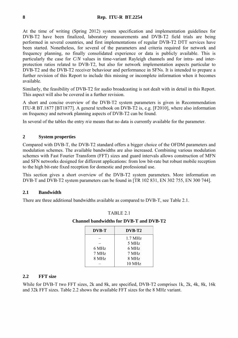
2.1 Bandwidth
There are three additional bandwidths available as compared to DVB-T, see Table 2.1.
TABLE 2.1
Channel bandwidths for DVB-T and DVB-T2
DVB-T DVB-T2
– –
6 MHz 7 MHz 8 MHz
–
1.7 MHz 5 MHz 6 MHz 7 MHz 8 MHz
10 MHz
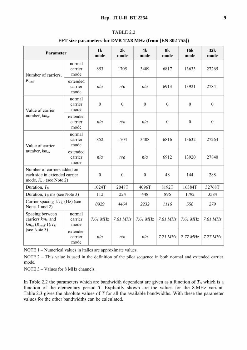
2.2 FFT size
While for DVB-T two FFT sizes, 2k and 8k, are specified, DVB-T2 comprises 1k, 2k, 4k, 8k, 16k and 32k FFT sizes. Table 2.2 shows the available FFT sizes for the 8 MHz variant.
Rep. ITU-R BT.2254 9
TABLE 2.2
FFT size parameters for DVB-T2/8 MHz (from [EN 302 755])
Parameter 1k
mode 2k
mode 4k
mode 8k
mode 16k
mode 32k
mode
Number of carriers, Ktotal
normal carrier mode
853 1705 3409 6817 13633 27265
extended carrier mode
n/a n/a n/a 6913 13921 27841
Value of carrier number, kmin
normal carrier mode
0 0 0 0 0 0
extended carrier mode
n/a n/a n/a 0 0 0
Value of carrier number, kmax
normal carrier mode
852 1704 3408 6816 13632 27264
extended carrier mode
n/a n/a n/a 6912 13920 27840
Number of carriers added on each side in extended carrier mode, Kext (see Note 2)
0 0 0 48 144 288
Duration, TU 1024T 2048T 4096T 8192T 16384T 32768T
Duration, TU ms (see Note 3) 112 224 448 896 1792 3584
Carrier spacing 1/TU (Hz) (see Notes 1 and 2)
8929 4464 2232 1116 558 279
Spacing between carriers kmin and kmax (Ktotal-1)/TU (see Note 3)
normal carrier mode
7.61 MHz 7.61 MHz 7.61 MHz 7.61 MHz 7.61 MHz 7.61 MHz
extended carrier mode
n/a n/a n/a 7.71 MHz 7.77 MHz 7.77 MHz
NOTE 1 – Numerical values in italics are approximate values.
NOTE 2 – This value is used in the definition of the pilot sequence in both normal and extended carrier mode.
NOTE 3 – Values for 8 MHz channels.
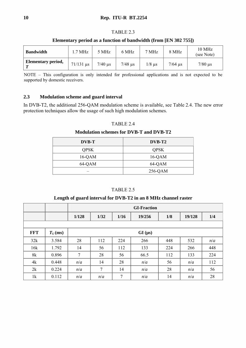
In Table 2.2 the parameters which are bandwidth dependent are given as a function of TU which is a function of the elementary period T. Explicitly shown are the values for the 8 MHz variant. Table 2.3 gives the absolute values of T for all the available bandwidths. With these the parameter values for the other bandwidths can be calculated.
10 Rep. ITU-R BT.2254
TABLE 2.3
Elementary period as a function of bandwidth (from [EN 302 755])
Bandwidth 1.7 MHz 5 MHz 6 MHz 7 MHz 8 MHz 10 MHz
(see Note)
Elementary period, T
71/131 µs 7/40 µs 7/48 µs 1/8 µs 7/64 µs 7/80 µs
NOTE – This configuration is only intended for professional applications and is not expected to be supported by domestic receivers.
2.3 Modulation scheme and guard interval
In DVB-T2, the additional 256-QAM modulation scheme is available, see Table 2.4. The new error protection techniques allow the usage of such high modulation schemes.
TABLE 2.4
Modulation schemes for DVB-T and DVB-T2
DVB-T DVB-T2
QPSK QPSK
16-QAM 16-QAM
64-QAM 64-QAM
– 256-QAM
TABLE 2.5
Length of guard interval for DVB-T2 in an 8 MHz channel raster
GI-Fraction
1/128 1/32 1/16 19/256 1/8 19/128 1/4
FFT TU (ms) GI (µs)
32k 3.584 28 112 224 266 448 532 n/a
16k 1.792 14 56 112 133 224 266 448
8k 0.896 7 28 56 66.5 112 133 224
4k 0.448 n/a 14 28 n/a 56 n/a 112
2k 0.224 n/a 7 14 n/a 28 n/a 56
1k 0.112 n/a n/a 7 n/a 14 n/a 28
Rep. ITU-R BT.2254 11
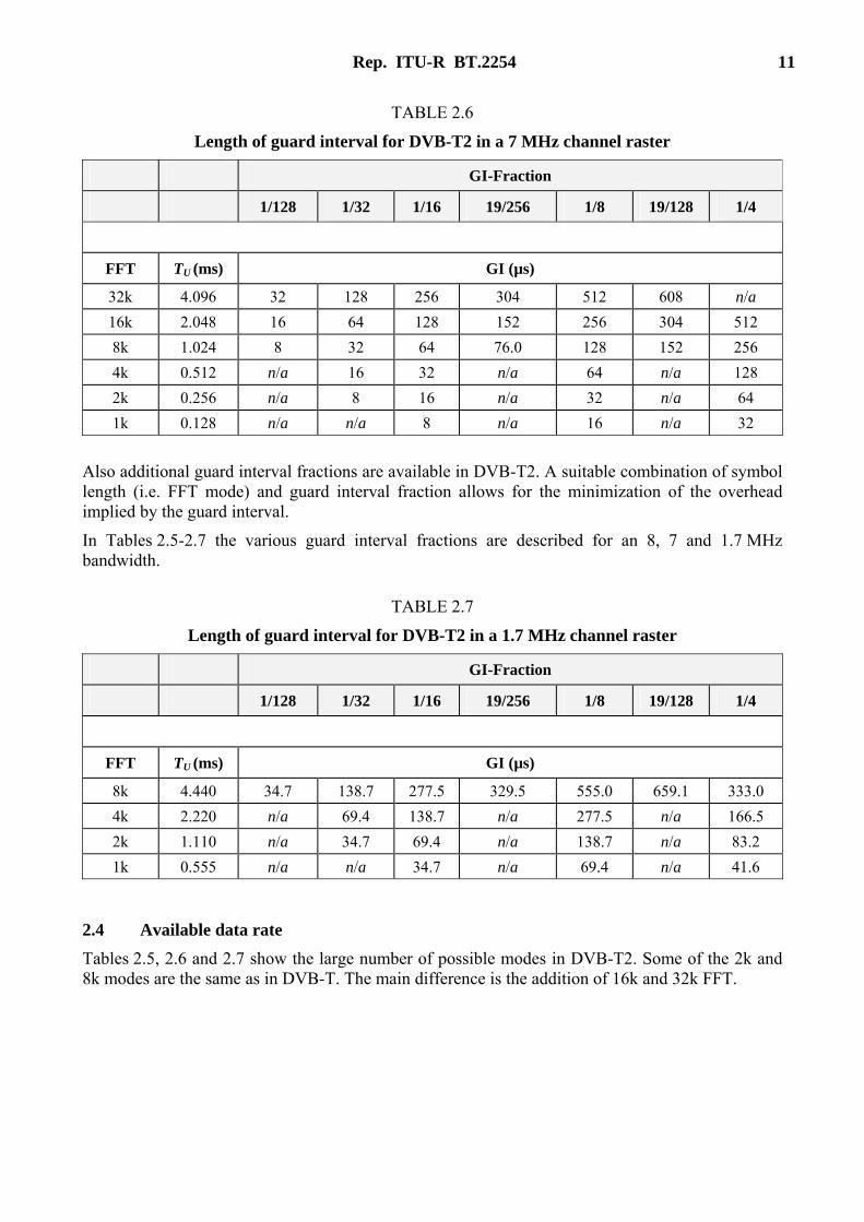
TABLE 2.6
Length of guard interval for DVB-T2 in a 7 MHz channel raster
GI-Fraction
1/128 1/32 1/16 19/256 1/8 19/128 1/4
FFT TU (ms) GI (µs)
32k 4.096 32 128 256 304 512 608 n/a
16k 2.048 16 64 128 152 256 304 512
8k 1.024 8 32 64 76.0 128 152 256
4k 0.512 n/a 16 32 n/a 64 n/a 128
2k 0.256 n/a 8 16 n/a 32 n/a 64
1k 0.128 n/a n/a 8 n/a 16 n/a 32
Also additional guard interval fractions are available in DVB-T2. A suitable combination of symbol length (i.e. FFT mode) and guard interval fraction allows for the minimization of the overhead implied by the guard interval.
In Tables 2.5-2.7 the various guard interval fractions are described for an 8, 7 and 1.7 MHz bandwidth.
TABLE 2.7
Length of guard interval for DVB-T2 in a 1.7 MHz channel raster
GI-Fraction
1/128 1/32 1/16 19/256 1/8 19/128 1/4
FFT TU (ms) GI (µs)
8k 4.440 34.7 138.7 277.5 329.5 555.0 659.1 333.0
4k 2.220 n/a 69.4 138.7 n/a 277.5 n/a 166.5
2k 1.110 n/a 34.7 69.4 n/a 138.7 n/a 83.2
1k 0.555 n/a n/a 34.7 n/a 69.4 n/a 41.6
2.4 Available data rate
Tables 2.5, 2.6 and 2.7 show the large number of possible modes in DVB-T2. Some of the 2k and 8k modes are the same as in DVB-T. The main difference is the addition of 16k and 32k FFT.
12 Rep. ITU-R BT.2254
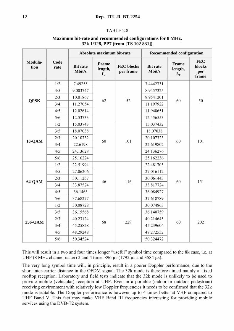
TABLE 2.8
Maximum bit-rate and recommended configurations for 8 MHz, 32k 1/128, PP7 (from [TS 102 831])
Modula-tion
Code rate
Absolute maximum bit-rate Recommended configuration
Bit rate Mbit/s
Frame length,
LF
FEC blocks per frame
Bit rate Mbit/s
Frame length,
LF
FEC blocks
per frame
QPSK
1/2 7.49255
62 52
7.4442731
60 50
3/5 9.003747 8.9457325
2/3 10.01867 9.9541201
3/4 11.27054 11.197922
4/5 12.02614 11.948651
5/6 12.53733 12.456553
16-QAM
1/2 15.03743
60 101
15.037432
60 101
3/5 18.07038 18.07038
2/3 20.10732 20.107323
3/4 22.6198 22.619802
4/5 24.13628 24.136276
5/6 25.16224 25.162236
64-QAM
1/2 22.51994
46 116
22.481705
60 151
3/5 27.06206 27.016112
2/3 30.11257 30.061443
3/4 33.87524 33.817724
4/5 36.1463 36.084927
5/6 37.68277 37.618789
256-QAM
1/2 30.08728
68 229
30.074863
60 202
3/5 36.15568 36.140759
2/3 40.23124 40.214645
3/4 45.25828 45.239604
4/5 48.29248 48.272552
5/6 50.34524 50.324472
This will result in a two and four times longer “useful” symbol time compared to the 8k case, i.e. at UHF (8 MHz channel raster) 2 and 4 times 896 µs (1792 µs and 3584 µs).
The very long symbol time will, in principle, result in a poorer Doppler performance, due to the short inter-carrier distance in the OFDM signal. The 32k mode is therefore aimed mainly at fixed rooftop reception. Laboratory and field tests indicate that the 32k mode is unlikely to be used to provide mobile (vehicular) reception at UHF. Even in a portable (indoor or outdoor pedestrian) receiving environment with relatively low Doppler frequencies it needs to be confirmed that the 32k mode is suitable. The Doppler performance is however up to 4 times better at VHF compared to UHF Band V. This fact may make VHF Band III frequencies interesting for providing mobile services using the DVB-T2 system.

Rep. ITU-R BT.2254 13
One additional difference between DVB-T and DVB-T2 is the increased number of GI fraction using 1/128, 19/256 and 19/128, which gives further possibilities to adopt the length of the guard interval to the size of the SFN.
As an example, Table 2.8 and Fig. 2.1 show the maximum bit-rate and recommended configurations for the system variant 8 MHz, 32k 1/128, PP7.
FIGURE 2.1
Maximum bit rate and bit rate for recommended configuration with 8 MHz bandwidth and 32k PP7 (from [TS 102 831])
A more comprehensive overview of the available data rates for the various DVB-T2 configurations is given in Annex 2.
Two parameters of the transmitted signal related to the FFT size of the OFDM modulation can influence planning of the DVB-T2 network:
– inter-carrier spacing;
– symbol duration.
Increasing the FFT size results in a narrower sub-carrier spacing and consequently in a longer symbol duration.
Further considerations on the suitable choice of a DVB-T2 configuration are described in § 2.11.
2.5 Carrier-to-noise ratio (C/N)
2.5.1 Introduction
The C/N characterizes the robustness of transmission systems with regard to noise and interference. As such it is used to determine the signal level required to receive a viable signal in noise and interference limited channels. Subsequently, the determination of the C/N is of fundamental importance for network planning.
0
10
20
30
40
50
60
1/2 3/5 2/3 3/4 4/5 5/6 1/2 3/5 2/3 3/4 4/5 5/6 1/2 3/5 2/3 3/4 4/5 5/6 1/2 3/5 2/3 3/4 4/5 5/6
4-QAM 16-QAM 64-QAM 256-QAM
Constellation and code-rate
Bitr
ate
(Mbi
t/s)
Maximum
Recommended
14 Rep. ITU-R BT.2254
At the time of writing insufficient measurements of receivers were available to provide an experimentally determined C/N representative of the receiver population. In lieu of measurements this section describes a methodology that can be used to calculate the C/N based upon the simulated receiver performance results provided in the DVB-T2 Implementation Guideline [TS 102 831]. The methodology proposed compares favourably with the limited measurements compiled to date in Annex 4, though it may be slightly conservative.
The methodology proposed here is similar to the one proposed for adoption in a coming update of the IEC 62216 E-book [IEC 62216] and aligns in general with the Nordig receiver specification [NorDig2010] without being identical with either of these two approaches. It is important to note that the C/N ratios derived using the following methodology are understood to describe the average behaviour of receivers which can be used for frequency and network planning. They are not intended to describe minimum receiver requirements in the sense of a specification.
This section also provides some background on the common reception channels that are encountered in broadcast network planning so that the correct C/N can be determined for the targeted receiving environment.
The full methodology for determining the C/N of a given mode and receiving environment is described below.
2.5.2 Methodology for the derivation of the C/N
The following main steps are usually necessary when determining the C/N to be used for planning:
– Step 1: Identify the target receive environment to determine the reception channel. This means identifying whether the network is aimed at fixed rooftop reception, portable indoor, portable outdoor or mobile reception, and for example, will lead to determining whether the C/N for a Ricean or Rayleigh channel is most appropriate.
– Step 2: Choose the DVB-T2 transmission mode. This step usually involves an iterative process where the requirements of capacity, coverage and cost are traded off or optimized. When a DVB-T2 mode is chosen, the simulation based C/N for a Gaussian channel (C/NGauss-raw) can be found in Table 2.9 and used as the base value for the proposed method.
– Step 3: Apply the methodology described in the following sections to adjust the identified C/NGauss-raw to correct it for real receiver implementation factors and to match it to the identified transmission channel and receiving environment.
2.5.3 Common reception channels
The main reception channels that are encountered in terrestrial broadcasting are briefly described below. Each of these will require a certain C/N that reflects how demanding the channel is for the receiver. The derivation of the final C/N is described in the following sections.
– Gaussian channel (AWGN): This channel is characterized by a single wanted signal with no channel perturbations where only Gaussian noise is present. It is the least demanding channel and is normally used only as a reference, not in practical network planning.
– Ricean channel: Used for planning fixed rooftop reception where there is predominantly a single direct signal and smaller amplitude reflections.
– Rayleigh channel(s):
i) Rayleigh static channel: Mainly used for planning portable indoor and outdoor reception. In this channel model the received signals consist only of a number of reflected signals – no direct signal is present. The simulations in the DVB-T2 ETSI Implementation Guideline [TS 102 831, Table 39] use a Rayleigh channel with 20 static paths. Due to the static nature of this channel model it should be regarded as a
Rep. ITU-R BT.2254 15
‘best case’ when planning for portable reception and should be used when the receiver is stationary.
ii) Rayleigh – slowly time varying, low Doppler frequency: This channel model should normally be used for planning portable outdoor and portable indoor reception, as slow channel variations cannot normally be avoided. Even if the receiver itself is stationary there are often other objects in the vicinity of the receiver which move, for example cars, trees or people. At low Doppler frequency the time interleaving in DVB-T2 is less effective, e.g. when the Doppler frequency is < 1/(interleaving time), this will normally result in a higher C/N compared to mobile reception at higher Doppler frequencies. This channel model is often considered to be a worst case for a DVB-T2 receiver.
iii) Rayleigh – mobile, high Doppler frequency: Used for planning mobile reception using external antenna or a handheld device. It should be noted that some DVB-T2 modes are not suitable for mobile reception, in particular the modulation 256-QAM and 32k. A profile particularly designed for mobile reception is DVB-T2-Lite which is described in Annex 5.
2.5.4 C/N for Gaussian channel
The following methodology has been proposed for adoption in a coming update of the IEC 62216 E-book [IEC 62216] and aligns with the Nordig receiver specification [NorDig2010].
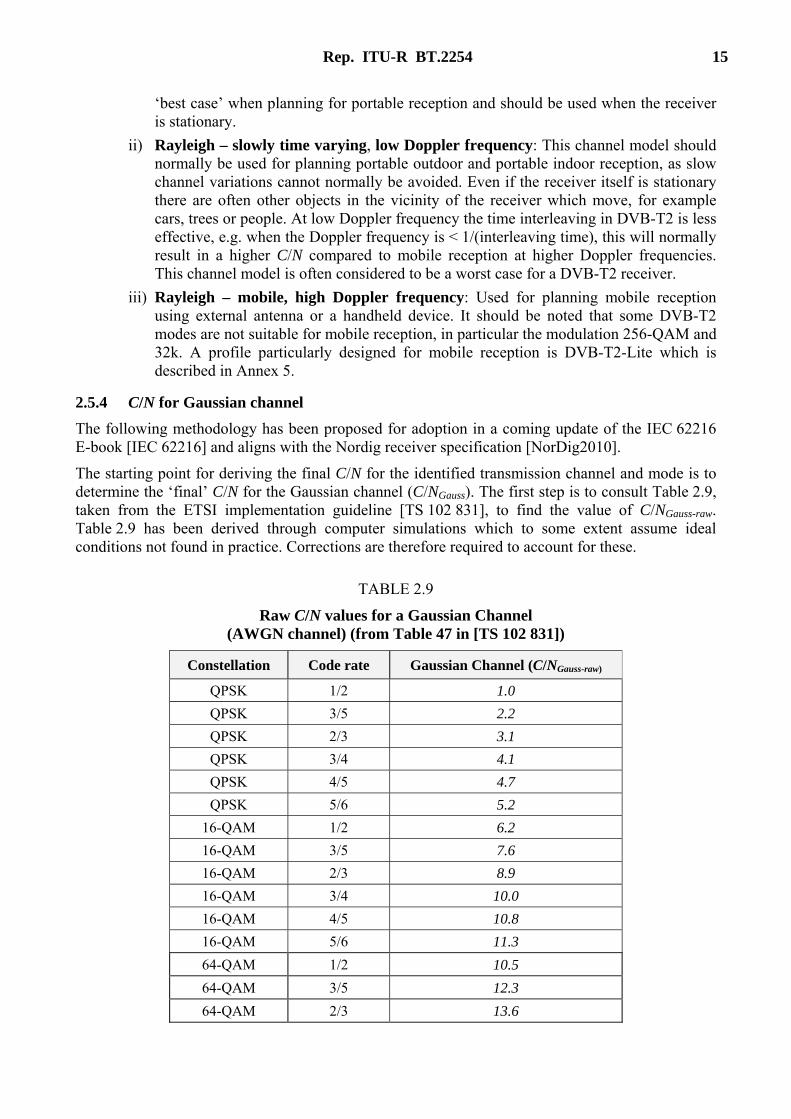
The starting point for deriving the final C/N for the identified transmission channel and mode is to determine the ‘final’ C/N for the Gaussian channel (C/NGauss). The first step is to consult Table 2.9, taken from the ETSI implementation guideline [TS 102 831], to find the value of C/NGauss-raw. Table 2.9 has been derived through computer simulations which to some extent assume ideal conditions not found in practice. Corrections are therefore required to account for these.
TABLE 2.9
Raw C/N values for a Gaussian Channel (AWGN channel) (from Table 47 in [TS 102 831])
Constellation Code rate Gaussian Channel (C/NGauss-raw)
QPSK 1/2 1.0
QPSK 3/5 2.2
QPSK 2/3 3.1
QPSK 3/4 4.1
QPSK 4/5 4.7
QPSK 5/6 5.2
16-QAM 1/2 6.2
16-QAM 3/5 7.6
16-QAM 2/3 8.9
16-QAM 3/4 10.0
16-QAM 4/5 10.8
16-QAM 5/6 11.3
64-QAM 1/2 10.5
64-QAM 3/5 12.3
64-QAM 2/3 13.6
16 Rep. ITU-R BT.2254
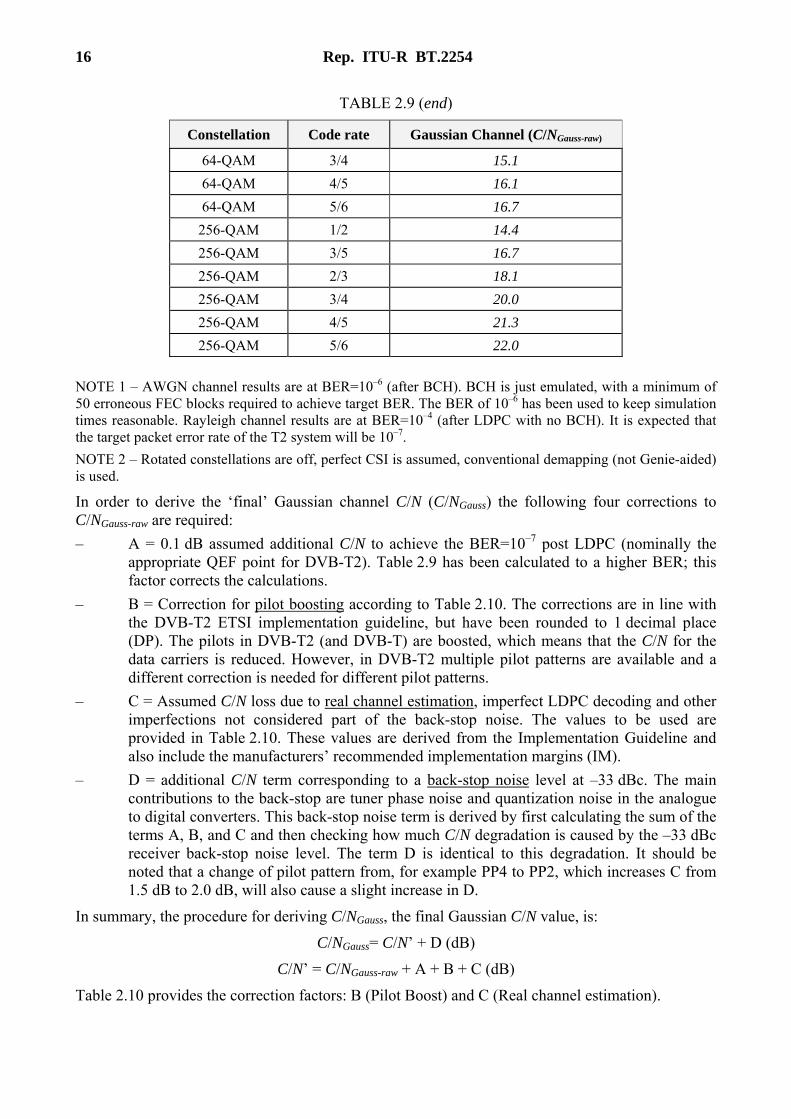
TABLE 2.9 (end)
Constellation Code rate Gaussian Channel (C/NGauss-raw)
64-QAM 3/4 15.1
64-QAM 4/5 16.1
64-QAM 5/6 16.7
256-QAM 1/2 14.4
256-QAM 3/5 16.7
256-QAM 2/3 18.1
256-QAM 3/4 20.0
256-QAM 4/5 21.3
256-QAM 5/6 22.0
NOTE 1 – AWGN channel results are at BER=10–6 (after BCH). BCH is just emulated, with a minimum of 50 erroneous FEC blocks required to achieve target BER. The BER of 10–6 has been used to keep simulation times reasonable. Rayleigh channel results are at BER=10–4 (after LDPC with no BCH). It is expected that the target packet error rate of the T2 system will be 10–7.
NOTE 2 – Rotated constellations are off, perfect CSI is assumed, conventional demapping (not Genie-aided) is used.
In order to derive the ‘final’ Gaussian channel C/N (C/NGauss) the following four corrections to C/NGauss-raw are required:
– A = 0.1 dB assumed additional C/N to achieve the BER=10–7 post LDPC (nominally the appropriate QEF point for DVB-T2). Table 2.9 has been calculated to a higher BER; this factor corrects the calculations.
– B = Correction for pilot boosting according to Table 2.10. The corrections are in line with the DVB-T2 ETSI implementation guideline, but have been rounded to 1 decimal place (DP). The pilots in DVB-T2 (and DVB-T) are boosted, which means that the C/N for the data carriers is reduced. However, in DVB-T2 multiple pilot patterns are available and a different correction is needed for different pilot patterns.
– C = Assumed C/N loss due to real channel estimation, imperfect LDPC decoding and other imperfections not considered part of the back-stop noise. The values to be used are provided in Table 2.10. These values are derived from the Implementation Guideline and also include the manufacturers’ recommended implementation margins (IM).
– D = additional C/N term corresponding to a back-stop noise level at –33 dBc. The main contributions to the back-stop are tuner phase noise and quantization noise in the analogue to digital converters. This back-stop noise term is derived by first calculating the sum of the terms A, B, and C and then checking how much C/N degradation is caused by the –33 dBc receiver back-stop noise level. The term D is identical to this degradation. It should be noted that a change of pilot pattern from, for example PP4 to PP2, which increases C from 1.5 dB to 2.0 dB, will also cause a slight increase in D.
In summary, the procedure for deriving C/NGauss, the final Gaussian C/N value, is:
C/NGauss= C/N’ + D (dB)
C/N’ = C/NGauss-raw + A + B + C (dB)
Table 2.10 provides the correction factors: B (Pilot Boost) and C (Real channel estimation).

Rep. ITU-R BT.2254 17
TABLE 2.10
Averaged C/N correction factors (in dB)*
Pilot Pattern PP1 PP2 PP3 PP4 PP5 PP6 PP7 PP8
A = BER 10–7 Correction 0.1 0.1 0.1 0.1 0.1 0.1 0.1 0.1
B = Pilot Boost Correction 0.4 0.4 0.5 0.5 0.5 0.5 0.3 0.4
C = Real Channel Estimation 2.0 2.0 1.5 1.5 1.0 1.0 1.0 1.0
* B has been rounded to 1 decimal place.
Some receivers may, in practice, perform slightly better, or slightly worse, than presented here, with the best receivers being perhaps 0.5-1 dB better, but this is likely to vary with receiver implementation and DVB-T2 mode. If it is thought the majority of receivers in a particular market will indeed perform better than above then the correction factor C could be reduced correspondingly. Making such a reduction would also cause a small change in D, which should be recalculated.
PP8 is a special case and should be considered with some caution. Refer to § 2.7 for more information.
Figure 2.2 shows D which quantifies the degradation in C/N for a back-stop noise level of –33 dBc. It is clear that for higher values of C/N, e.g. for high-order modulation schemes and code rates, D can become significant, and should be taken into account.
FIGURE 2.2
Factor D, C/N degradation for a back-stop noise level of –33 dBc, see [EDP-T7]
TABLE 2.11
Factor D, C/N degradation as table for C/N values from 15 to 32
C/N (dB) 15 16 17 18 19 20 21 22 23 24 25 26 27 28 29 30 31 32
D (dB) 0.07 0.09 0.11 0.14 0.18 0.22 0.28 0.36 0.46 0.58 0.75 0.97 1.26 1.65 2.20 3.02 4.33 6.87
18 Rep. ITU-R BT.2254
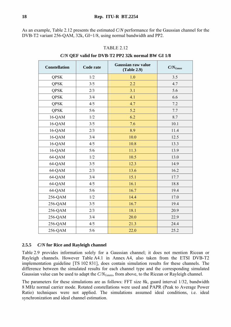
As an example, Table 2.12 presents the estimated C/N performance for the Gaussian channel for the DVB-T2 variant 256-QAM, 32k, GI=1/8, using normal bandwidth and PP2.
TABLE 2.12
C/N QEF valid for DVB-T2 PP2 32k normal BW GI 1/8
Constellation Code rate Gaussian raw value
(Table 2.9) C/NGauss
QPSK 1/2 1.0 3.5
QPSK 3/5 2.2 4.7
QPSK 2/3 3.1 5.6
QPSK 3/4 4.1 6.6
QPSK 4/5 4.7 7.2
QPSK 5/6 5.2 7.7
16-QAM 1/2 6.2 8.7
16-QAM 3/5 7.6 10.1
16-QAM 2/3 8.9 11.4
16-QAM 3/4 10.0 12.5
16-QAM 4/5 10.8 13.3
16-QAM 5/6 11.3 13.9
64-QAM 1/2 10.5 13.0
64-QAM 3/5 12.3 14.9
64-QAM 2/3 13.6 16.2
64-QAM 3/4 15.1 17.7
64-QAM 4/5 16.1 18.8
64-QAM 5/6 16.7 19.4
256-QAM 1/2 14.4 17.0
256-QAM 3/5 16.7 19.4
256-QAM 2/3 18.1 20.9
256-QAM 3/4 20.0 22.9
256-QAM 4/5 21.3 24.4
256-QAM 5/6 22.0 25.2
2.5.5 C/N for Rice and Rayleigh channel
Table 2.9 provides information solely for a Gaussian channel; it does not mention Ricean or Rayleigh channels. However Table A4.1 in Annex A4, also taken from the ETSI DVB-T2 implementation guideline [TS 102 831], does contain simulation results for these channels. The difference between the simulated results for each channel type and the corresponding simulated Gaussian value can be used to adapt the C/NGauss, from above, to the Ricean or Rayleigh channel.
The parameters for these simulations are as follows: FFT size 8k, guard interval 1/32, bandwidth 8 MHz normal carrier mode. Rotated constellations were used and PAPR (Peak to Average Power Ratio) techniques were not applied. The simulations assumed ideal conditions, i.e. ideal synchronization and ideal channel estimation.

Rep. ITU-R BT.2254 19
The results are given at a BER of 10–7 after LDPC, corresponding to approximately 10–11 after BCH, where an LDPC block length of 64,800 was used. The channel models used for the simulation are described in detail in [TS 102 831, § 14.2].
The difference in required C/N is 0.2 to 0.5 dB when comparing the Gaussian and Ricean channels, and 1.0-3.4 dB when comparing the Gaussian and the Rayleigh values. The larger increases are found for the less robust modes using higher order modulation and codes rates.
Adding this difference to the C/NGauss-raw from Table 2.9 and following the procedure of § 2.5.4 for the corrections, C/N values for the Ricean and the Rayleigh cases can be derived:
C/N’Rice = C/NGauss-raw + DELTARice +A + B + C
C/NRice = C/N’Rice + D
C/N’Rayleigh = C/NGauss-raw + DELTARayleigh + A + B +C
C/NRayleigh = C/N’Rayleigh + D
where DELTA is given in Table 2.13.
TABLE 2.13
Increase DELTA (dB) of C/N for Rice and static Rayleigh channels with regard to Gaussian channel
Constellation Code rate DELTA C/NRice (dB) DELTA C/NRayleigh (dB)
QPSK 1/2 0.2 1.0
QPSK 3/5 0.2 1.3
QPSK 2/3 0.3 1.8
QPSK 3/4 0.3 2.1
QPSK 4/5 0.3 2.4
QPSK 5/6 0.4 2.7
16-QAM 1/2 0.2 1.5
16-QAM 3/5 0.2 1.7
16-QAM 2/3 0.2 1.9
16-QAM 3/4 0.4 2.4
16-QAM 4/5 0.4 2.8
16-QAM 5/6 0.4 3.1
64-QAM 1/2 0.3 2.0
64-QAM 3/5 0.3 2.0
64-QAM 2/3 0.3 2.1
64-QAM 3/4 0.3 2.6
64-QAM 4/5 0.5 3.1
64-QAM 5/6 0.4 3.4
256-QAM 1/2 0.4 2.4
256-QAM 3/5 0.2 2.2
256-QAM 2/3 0.3 2.3
20 Rep. ITU-R BT.2254
TABLE 2.13 (end)
Constellation Code Rate DELTA C/NRice (dB) DELTA C/NRayleigh (dB)
256-QAM 3/4 0.3 2.6
256-QAM 4/5 0.4 3.0
256-QAM 5/6 0.4 3.4
Simulations for a LDPC block length of 16,200 give similar results for the difference between Gaussian and Rice or Rayleigh channel, see Implementation Guideline [TS 102 831].
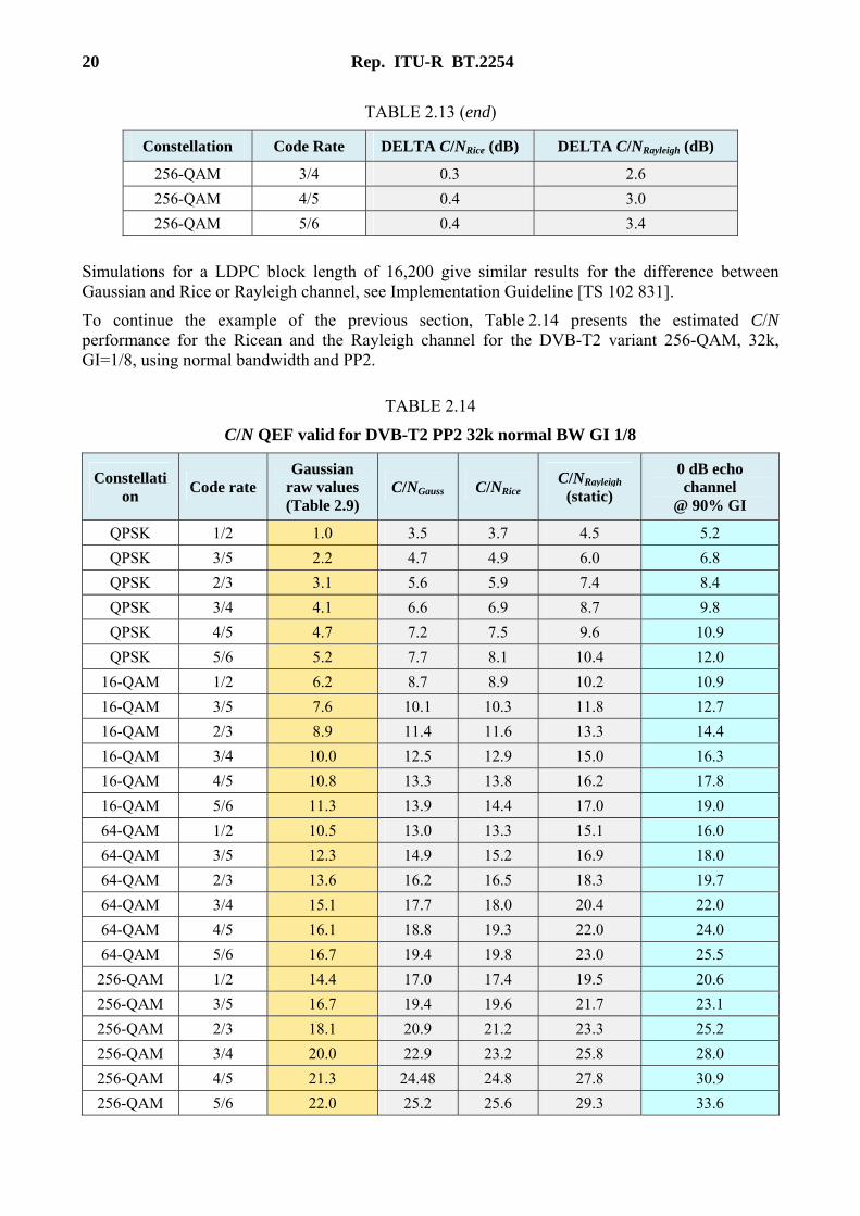
To continue the example of the previous section, Table 2.14 presents the estimated C/N performance for the Ricean and the Rayleigh channel for the DVB-T2 variant 256-QAM, 32k, GI=1/8, using normal bandwidth and PP2.
TABLE 2.14
C/N QEF valid for DVB-T2 PP2 32k normal BW GI 1/8
Constellation
Code rate Gaussian
raw values (Table 2.9)
C/NGauss C/NRice C/NRayleigh
(static)
0 dB echo channel
@ 90% GI
QPSK 1/2 1.0 3.5 3.7 4.5 5.2
QPSK 3/5 2.2 4.7 4.9 6.0 6.8
QPSK 2/3 3.1 5.6 5.9 7.4 8.4
QPSK 3/4 4.1 6.6 6.9 8.7 9.8
QPSK 4/5 4.7 7.2 7.5 9.6 10.9
QPSK 5/6 5.2 7.7 8.1 10.4 12.0
16-QAM 1/2 6.2 8.7 8.9 10.2 10.9
16-QAM 3/5 7.6 10.1 10.3 11.8 12.7
16-QAM 2/3 8.9 11.4 11.6 13.3 14.4
16-QAM 3/4 10.0 12.5 12.9 15.0 16.3
16-QAM 4/5 10.8 13.3 13.8 16.2 17.8
16-QAM 5/6 11.3 13.9 14.4 17.0 19.0
64-QAM 1/2 10.5 13.0 13.3 15.1 16.0
64-QAM 3/5 12.3 14.9 15.2 16.9 18.0
64-QAM 2/3 13.6 16.2 16.5 18.3 19.7
64-QAM 3/4 15.1 17.7 18.0 20.4 22.0
64-QAM 4/5 16.1 18.8 19.3 22.0 24.0
64-QAM 5/6 16.7 19.4 19.8 23.0 25.5
256-QAM 1/2 14.4 17.0 17.4 19.5 20.6
256-QAM 3/5 16.7 19.4 19.6 21.7 23.1
256-QAM 2/3 18.1 20.9 21.2 23.3 25.2
256-QAM 3/4 20.0 22.9 23.2 25.8 28.0
256-QAM 4/5 21.3 24.48 24.8 27.8 30.9
256-QAM 5/6 22.0 25.2 25.6 29.3 33.6
Rep. ITU-R BT.2254 21
For information, Table 2.14 also contains expected 0 dB echo performance at 90% of the guard interval length. These values are calculated using the same principle as previously described, by adding the difference between the C/N Gaussian and simulated C/N 0 dB from Table A4.1 in Annex A4 to the previously derived C/N for the Gaussian channel.
However, additional code rate dependant degradation needs to be added in the 0 dB echo case. This degradation factor is given in Table 2.15.
TABLE 2.15
Additional code rate dependant C/N degradation for 0 dB echo profile
Code rate 1/2 3/5 2/3 3/4 4/5 5/6
Additional degradation (dB) 1.0 1.2 1.4 1.6 1.8 2.0
The 0 dB echoes profile is mainly used for testing of receiver performance, since it is considered as a worst case. However, strong echoes or echoes where the echo level is the same as the wanted (0 dB echoes) can occur in practice, most commonly in SFNs.
In such cases the receiver would require an additional margin up to the limit set out in Table 2.15, depending on the echo delay and magnitude. The worst condition occurs when two signals from two transmitters arrive with the same amplitude at the receiver. In this case, the channel frequency response of the received signal presents a periodic fading pattern with frequency dependant on the inverse of the relative delay between echoes. The impact on the receiver will depend strongly on the pilot pattern and on the channel estimation algorithm [Po2005, EPB2011].
From experience with DVB-T and DVB-H it can be expected that the C/N for DVB-T2 in a time-variant Rayleigh channel would be higher than those for a static Rayleigh channel. But, depending upon the receiver performance, variations can be expected. For low Doppler frequencies, significantly higher C/N values can be expected since the time interleaving in DVB-T2 is not effective at low Doppler frequencies < 1/(interleaving time).
Annex 4 compares the results obtained from applying this methodology to measurements of a restricted sample of DVB-T2 receivers. This comparison indicates that the methodology derived C/N ratios of this section are perhaps conservative with respect to certain DVB-T2 modes and receiving environments. If further measurements confirm these findings a refinement of the approach may be considered.
2.6 Rotated constellation
2.6.1 Concept
In DVB-T2 a performance improvement with regard to DVB-T is achieved by treating the constellation diagram of the channel symbols in a more flexible way. A rotation of the constellation diagram is applied which yields an improvement. Here, the description of this approach follows the presentation given by [ND2007, ND2008]. Also the results quoted in § 2.6.6 are taken from these references; they are theoretical results assuming ideal receiver behaviour.
2.6.2 Constellation diagram
In DVB-T2 modulation, an information frame is encoded via a binary outer FEC code, then processed by a bit interleaver and the resulting sequence is mapped to a succession of complex channel symbols. Such a channel symbol is composed of an in-phase (I) and a quadrature (Q) component, represented in a constellation diagram as shown in Fig. 2.3. A symbol carries m bits

22 Rep. ITU-R BT.2254
according to the chosen 2m-ary constellation characteristics. In QPSK a symbol carries two bits, in 16-QAM it carries 4 bits, in 64-QAM it carries 6 bits, etc.
FIGURE 2.3
Constellation diagram for 16-QAM modulation
(Figure taken from [ND2008])
There are various ways of attributing the bits to the symbols. Best results are achieved if only one bit is changed when going from one symbol to the next closest symbol. In this way only one bit is mistaken when a symbol mismatch occurs with the next closest symbol. This coding is called Gray mapping. Figure 2.3 shows a Gray mapping constellation.
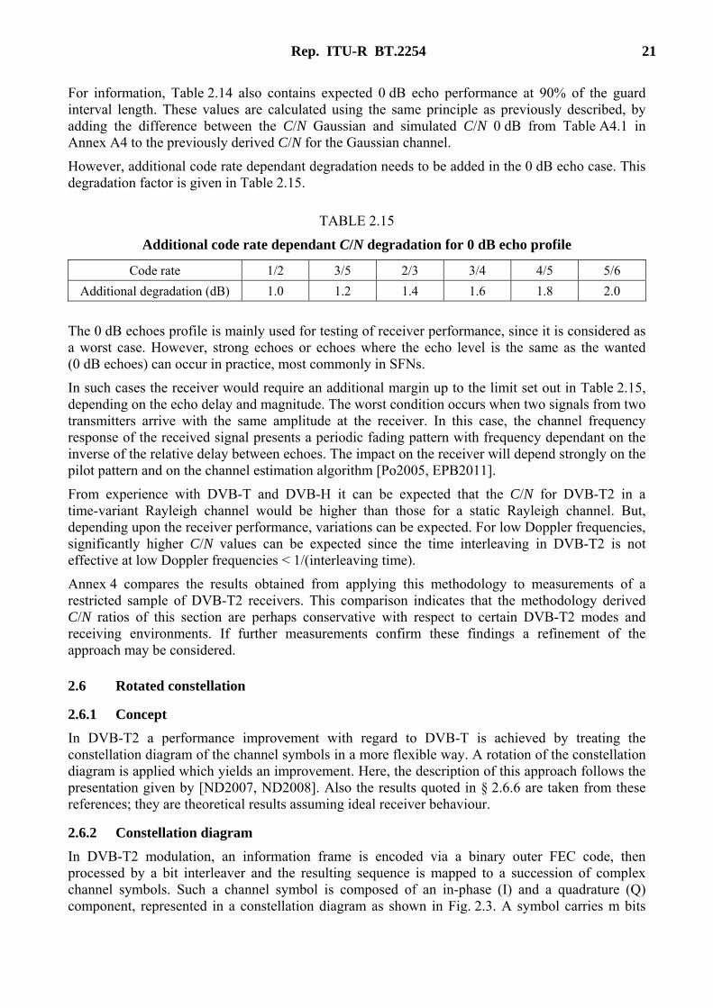
2.6.3 Rotation of the constellation diagram
Gray mapping implies an independence of I and Q components of the symbol. As a consequence, all constellation points need both I and Q components to be identified. I contains no information about Q and vice versa. One way of avoiding this independence is to rotate the constellation diagram, as shown in Fig. 2.4. Now each single m-bit has an individual I and Q component.
Rep. ITU-R BT.2254 23
FIGURE 2.4
Rotated constellation diagram for 16-QAM modulation
(from [TS 102 831])
2.6.4 Rotation angle
In order to determine the optimal rotation angle various aspects have to be considered. Generally, the projection of the constellation points on one axis should have equal distance to gain the best performance. This is best achieved with the rotation angles given in Table 2.16.
TABLE 2.16
Values of the rotation angle
Constellation Rotation angle (degrees)
QPSK 29.0
16-QAM 16.8
64-QAM 8.6
256-QAM 3.6
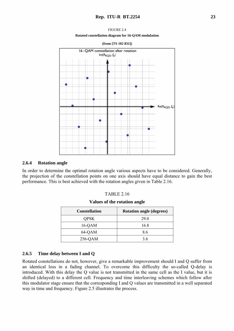
2.6.5 Time delay between I and Q
Rotated constellations do not, however, give a remarkable improvement should I and Q suffer from an identical loss in a fading channel. To overcome this difficulty the so-called Q-delay is introduced. With this delay the Q value is not transmitted in the same cell as the I value, but it is shifted (delayed) to a different cell. Frequency and time interleaving schemes which follow after this modulator stage ensure that the corresponding I and Q values are transmitted in a well separated way in time and frequency. Figure 2.5 illustrates the process.
24 Rep. ITU-R BT.2254
FIGURE 2.5
Structure of bit interleaved coded modulation with rotated-QAM mapper and delay
(Figure taken from [F2010])
A cell is the result of mapping a later carrier. In contrast to DVB-T, mapping is not carried out after all interleaving processes but relatively early, after the error protection and after the bit interleaver. However, this is still followed by the cell interleaver, the time interleaver and the frequency interleaver which is the reason why the mapping result cannot yet be allocated to a carrier and why the term “cell” was introduced. A cell is, therefore, a complex number consisting of an I-component and a Q-component, i.e. a real part and an imaginary part. For more details see [F2010].
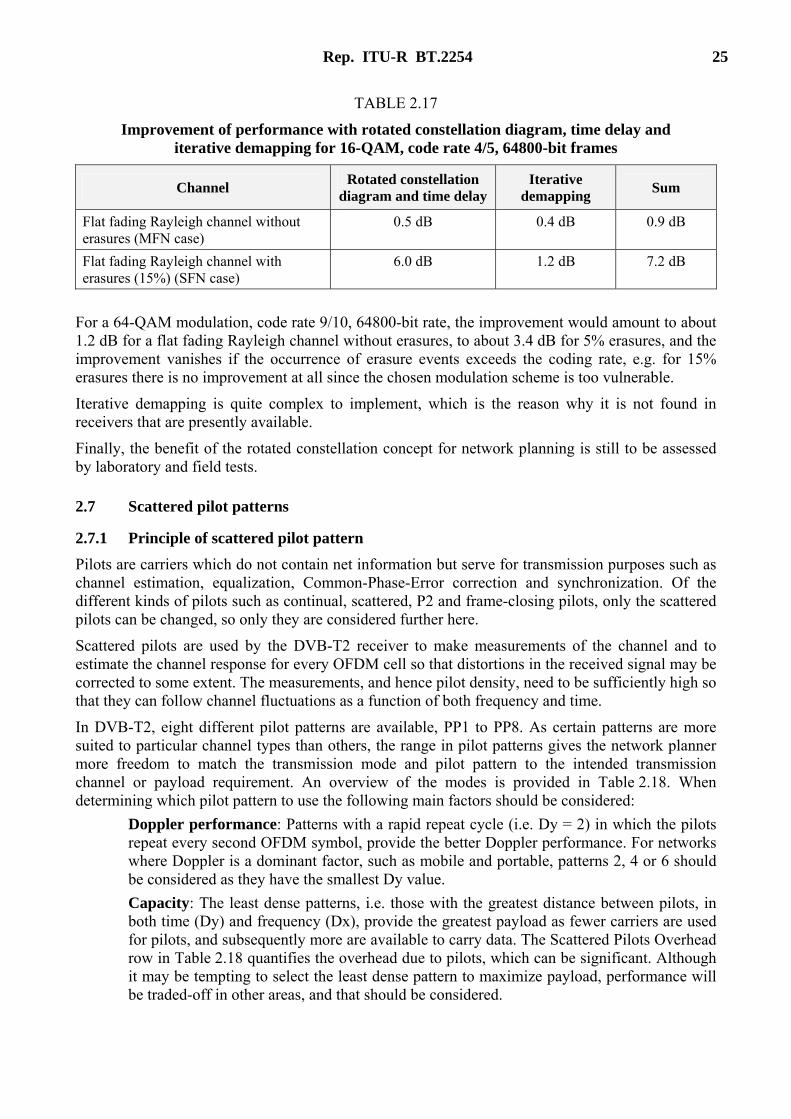
2.6.6 Improvement of performance
For a 16-QAM modulation, code rate 4/5 and 64800-bit frames, simulations indicate that the application of a rotated constellation diagram provides an improvement of performance of about 0.5 dB for a flat fading Rayleigh channel without erasures, relevant for an MFN. This is not a remarkable improvement. However, for a flat fading Rayleigh channel with erasures (15% assumed), relevant for SFN, an improvement of about 6 dB is predicted, which would be remarkable, see Table 2.14.
This 6 dB result is based on a simulation that uses ideal identification of erasures, which allows the decoding/demapping algorithms to make the maximum coding gain. In a real receiver, identifying erasures is extremely difficult because they are affected by noise, so in practice these gains are not achievable.
There exists an additional technique, iterative demapping, which may improve the performance by another 0.4 dB for a flat fading Rayleigh channel without erasures and 1.2 dB for a flat fading Rayleigh channel with erasures, see Table 2.17.
Rep. ITU-R BT.2254 25
TABLE 2.17
Improvement of performance with rotated constellation diagram, time delay and iterative demapping for 16-QAM, code rate 4/5, 64800-bit frames
Channel Rotated constellation
diagram and time delay Iterative
demapping Sum
Flat fading Rayleigh channel without erasures (MFN case)
0.5 dB 0.4 dB 0.9 dB
Flat fading Rayleigh channel with erasures (15%) (SFN case)
6.0 dB 1.2 dB 7.2 dB
For a 64-QAM modulation, code rate 9/10, 64800-bit rate, the improvement would amount to about 1.2 dB for a flat fading Rayleigh channel without erasures, to about 3.4 dB for 5% erasures, and the improvement vanishes if the occurrence of erasure events exceeds the coding rate, e.g. for 15% erasures there is no improvement at all since the chosen modulation scheme is too vulnerable.
Iterative demapping is quite complex to implement, which is the reason why it is not found in receivers that are presently available.
Finally, the benefit of the rotated constellation concept for network planning is still to be assessed by laboratory and field tests.
2.7 Scattered pilot patterns
2.7.1 Principle of scattered pilot pattern
Pilots are carriers which do not contain net information but serve for transmission purposes such as channel estimation, equalization, Common-Phase-Error correction and synchronization. Of the different kinds of pilots such as continual, scattered, P2 and frame-closing pilots, only the scattered pilots can be changed, so only they are considered further here.
Scattered pilots are used by the DVB-T2 receiver to make measurements of the channel and to estimate the channel response for every OFDM cell so that distortions in the received signal may be corrected to some extent. The measurements, and hence pilot density, need to be sufficiently high so that they can follow channel fluctuations as a function of both frequency and time.
In DVB-T2, eight different pilot patterns are available, PP1 to PP8. As certain patterns are more suited to particular channel types than others, the range in pilot patterns gives the network planner more freedom to match the transmission mode and pilot pattern to the intended transmission channel or payload requirement. An overview of the modes is provided in Table 2.18. When determining which pilot pattern to use the following main factors should be considered:
Doppler performance: Patterns with a rapid repeat cycle (i.e. Dy = 2) in which the pilots repeat every second OFDM symbol, provide the better Doppler performance. For networks where Doppler is a dominant factor, such as mobile and portable, patterns 2, 4 or 6 should be considered as they have the smallest Dy value.
Capacity: The least dense patterns, i.e. those with the greatest distance between pilots, in both time (Dy) and frequency (Dx), provide the greatest payload as fewer carriers are used for pilots, and subsequently more are available to carry data. The Scattered Pilots Overhead row in Table 2.18 quantifies the overhead due to pilots, which can be significant. Although it may be tempting to select the least dense pattern to maximize payload, performance will be traded-off in other areas, and that should be considered.
26 Rep. ITU-R BT.2254
FFT Size and Guard Interval: Only a subset of pilot patterns is permitted for every FFT size and Guard Interval combination – these are shown in Table 2.19. The Table is valid only for SISO (single input single output) of DVB-T2. A different Table applies to MISO (multiple input single output) which is described in detail in § 4.3.
C/N: Section 2.5 presents a method for determining the C/N for different transmission modes. In that section it is shown that the C/N is dependent on the pilot pattern and that the denser patterns require a higher C/N than those with a lower density. If the C/N is a dominant factor then lower density patterns, such as PP6 and PP7 could be considered, though the benefit is marginal.
The small distance (Dx) of the pilots in PP1 proves this pattern as most robust against inter-symbol interference, whereas PP6 and PP7 are most vulnerable to it.
PP8 – Receiver Capability: Pilot pattern 8 requires the receiver to employ a channel equalization strategy that is fundamentally different to the others – PP8 channel estimation is based on the data rather than the pilots. No receivers are known to have incorporated this mode, largely due to the additional complexity required in the receiver. Therefore before settling on this pattern, receivers intended for the service should be confirmed to support it. Furthermore PP8 has some limitations over the others that should be considered. PLPs are not supported in PP8, and time interleaving should not be used – the latter means that the vastly improved impulse resilience of DVB-T2, a significantly important benefit, cannot be realized. More detailed information regarding this mode, its benefits and limitations, can be found in §§ 5.4 and 10.3.2.3.5.4 and 16.2.4.5.6 of the implementation guidelines [TS 102 831], should it be required.
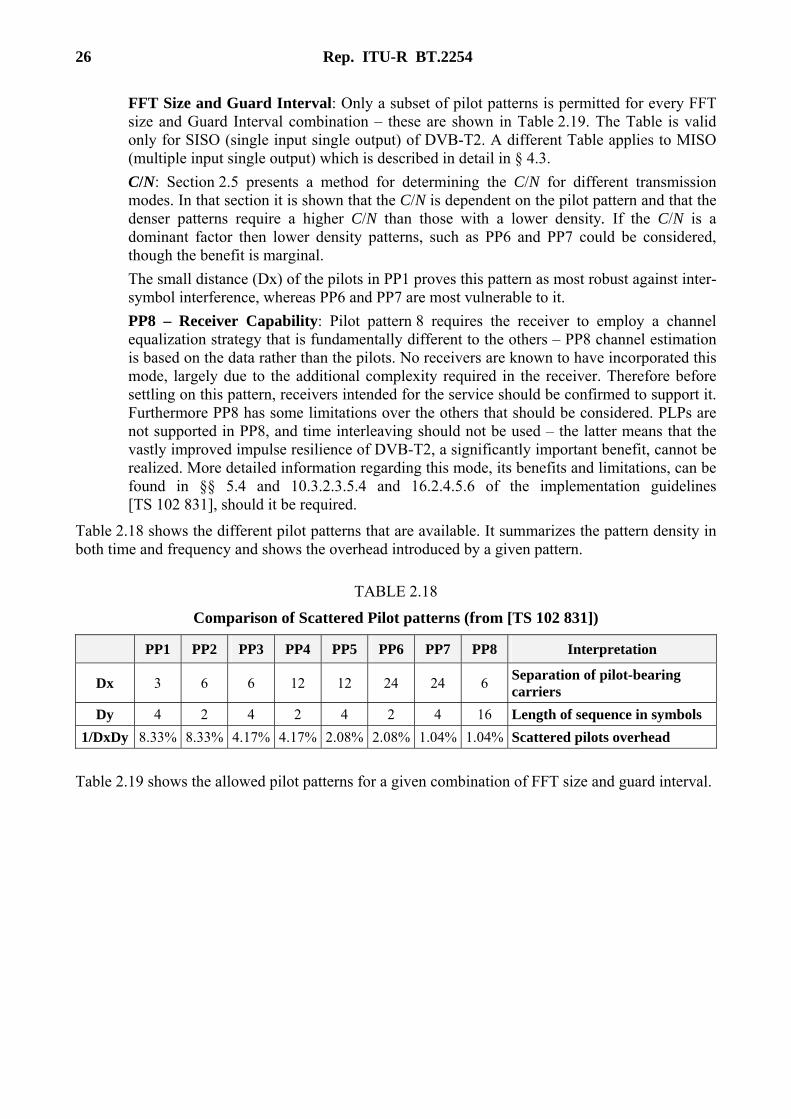
Table 2.18 shows the different pilot patterns that are available. It summarizes the pattern density in both time and frequency and shows the overhead introduced by a given pattern.
TABLE 2.18
Comparison of Scattered Pilot patterns (from [TS 102 831])
PP1 PP2 PP3 PP4 PP5 PP6 PP7 PP8 Interpretation
Dx 3 6 6 12 12 24 24 6 Separation of pilot-bearing carriers
Dy 4 2 4 2 4 2 4 16 Length of sequence in symbols
1/DxDy 8.33% 8.33% 4.17% 4.17% 2.08% 2.08% 1.04% 1.04% Scattered pilots overhead
Table 2.19 shows the allowed pilot patterns for a given combination of FFT size and guard interval.
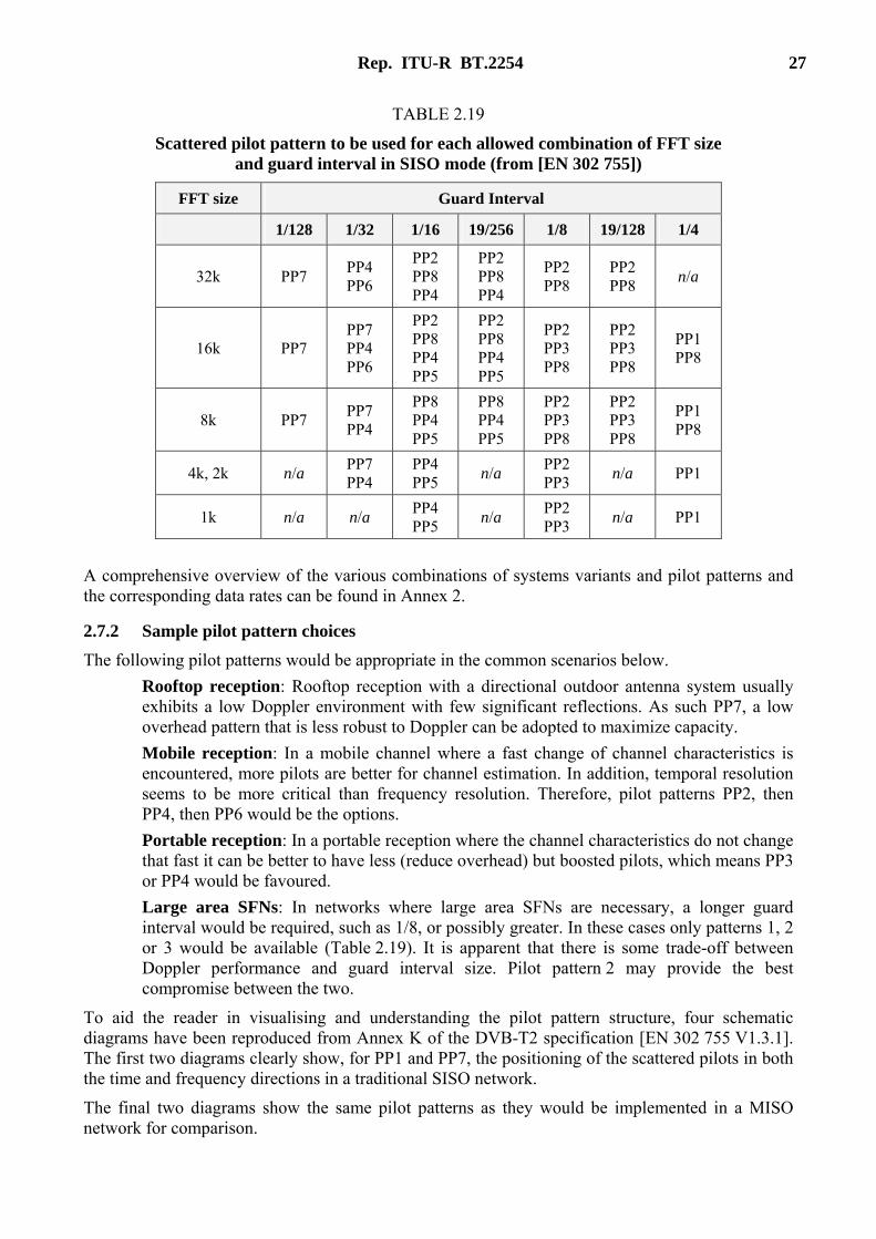
Rep. ITU-R BT.2254 27
TABLE 2.19
Scattered pilot pattern to be used for each allowed combination of FFT size and guard interval in SISO mode (from [EN 302 755])
FFT size Guard Interval
1/128 1/32 1/16 19/256 1/8 19/128 1/4
32k PP7 PP4 PP6
PP2 PP8 PP4
PP2 PP8 PP4
PP2 PP8
PP2 PP8
n/a
16k PP7 PP7 PP4 PP6
PP2 PP8 PP4 PP5
PP2 PP8 PP4 PP5
PP2 PP3 PP8
PP2 PP3 PP8
PP1 PP8
8k PP7 PP7 PP4
PP8 PP4 PP5
PP8 PP4 PP5
PP2 PP3 PP8
PP2 PP3 PP8
PP1 PP8
4k, 2k n/a PP7 PP4
PP4 PP5
n/a PP2 PP3
n/a PP1
1k n/a n/a PP4 PP5
n/a PP2 PP3
n/a PP1
A comprehensive overview of the various combinations of systems variants and pilot patterns and the corresponding data rates can be found in Annex 2.
2.7.2 Sample pilot pattern choices
The following pilot patterns would be appropriate in the common scenarios below.
Rooftop reception: Rooftop reception with a directional outdoor antenna system usually exhibits a low Doppler environment with few significant reflections. As such PP7, a low overhead pattern that is less robust to Doppler can be adopted to maximize capacity.
Mobile reception: In a mobile channel where a fast change of channel characteristics is encountered, more pilots are better for channel estimation. In addition, temporal resolution seems to be more critical than frequency resolution. Therefore, pilot patterns PP2, then PP4, then PP6 would be the options.
Portable reception: In a portable reception where the channel characteristics do not change that fast it can be better to have less (reduce overhead) but boosted pilots, which means PP3 or PP4 would be favoured.
Large area SFNs: In networks where large area SFNs are necessary, a longer guard interval would be required, such as 1/8, or possibly greater. In these cases only patterns 1, 2 or 3 would be available (Table 2.19). It is apparent that there is some trade-off between Doppler performance and guard interval size. Pilot pattern 2 may provide the best compromise between the two.
To aid the reader in visualising and understanding the pilot pattern structure, four schematic diagrams have been reproduced from Annex K of the DVB-T2 specification [EN 302 755 V1.3.1]. The first two diagrams clearly show, for PP1 and PP7, the positioning of the scattered pilots in both the time and frequency directions in a traditional SISO network.
The final two diagrams show the same pilot patterns as they would be implemented in a MISO network for comparison.

28 Rep. ITU-R BT.2254
FIGURE 2.6
Pilot pattern 1 – SISO (from [EN 302 755 V1.3.1])
FIGURE 2.7
Pilot pattern 7 – SISO (from [EN 302 755 V1.3.1])
FIGURE 2.8
Pilot pattern 1 – MISO (from [EN 302 755 V1.3.1])
Rep. ITU-R BT.2254 29
FIGURE 2.9
Pilot pattern 7 – MISO (from [EN 302 755 V1.3.1])
2.8 Time interleaving
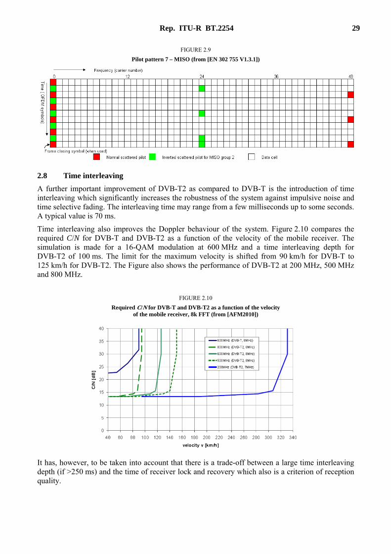
A further important improvement of DVB-T2 as compared to DVB-T is the introduction of time interleaving which significantly increases the robustness of the system against impulsive noise and time selective fading. The interleaving time may range from a few milliseconds up to some seconds. A typical value is 70 ms.
Time interleaving also improves the Doppler behaviour of the system. Figure 2.10 compares the required C/N for DVB-T and DVB-T2 as a function of the velocity of the mobile receiver. The simulation is made for a 16-QAM modulation at 600 MHz and a time interleaving depth for DVB-T2 of 100 ms. The limit for the maximum velocity is shifted from 90 km/h for DVB-T to 125 km/h for DVB-T2. The Figure also shows the performance of DVB-T2 at 200 MHz, 500 MHz and 800 MHz.
FIGURE 2.10
Required C/N for DVB-T and DVB-T2 as a function of the velocity of the mobile receiver, 8k FFT (from [AFM2010])
It has, however, to be taken into account that there is a trade-off between a large time interleaving depth (if >250 ms) and the time of receiver lock and recovery which also is a criterion of reception quality.
30 Rep. ITU-R BT.2254
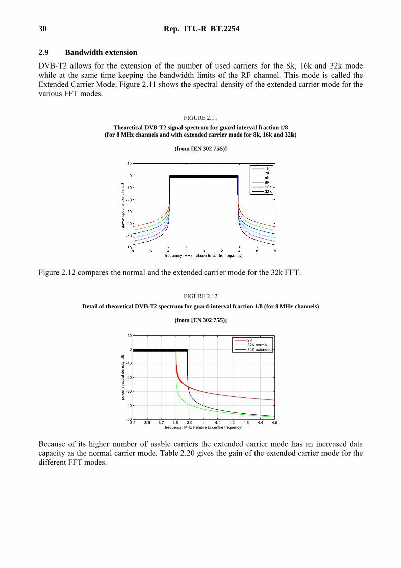
2.9 Bandwidth extension
DVB-T2 allows for the extension of the number of used carriers for the 8k, 16k and 32k mode while at the same time keeping the bandwidth limits of the RF channel. This mode is called the Extended Carrier Mode. Figure 2.11 shows the spectral density of the extended carrier mode for the various FFT modes.
FIGURE 2.11
Theoretical DVB-T2 signal spectrum for guard interval fraction 1/8 (for 8 MHz channels and with extended carrier mode for 8k, 16k and 32k)
(from [EN 302 755)]
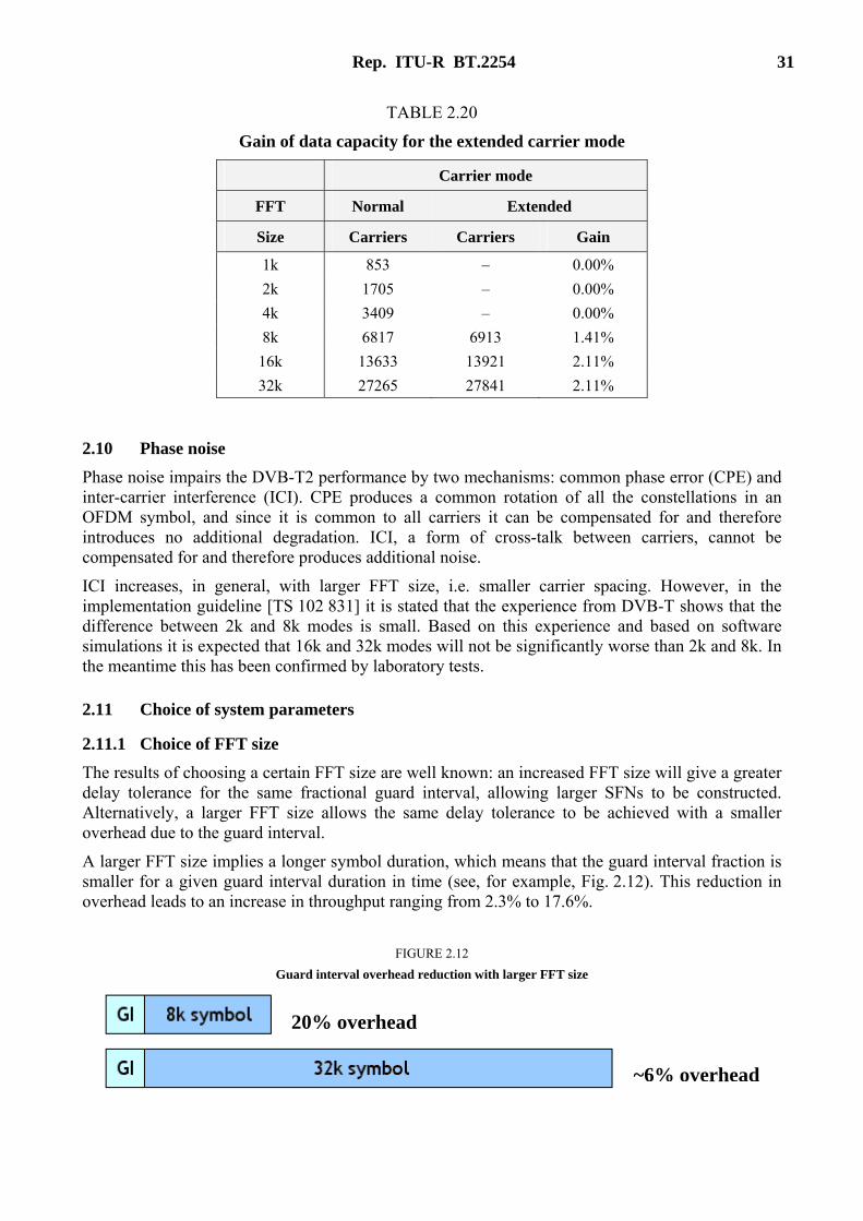
Figure 2.12 compares the normal and the extended carrier mode for the 32k FFT.
FIGURE 2.12
Detail of theoretical DVB-T2 spectrum for guard-interval fraction 1/8 (for 8 MHz channels)
(from [EN 302 755)]
Because of its higher number of usable carriers the extended carrier mode has an increased data capacity as the normal carrier mode. Table 2.20 gives the gain of the extended carrier mode for the different FFT modes.
Rep. ITU-R BT.2254 31
TABLE 2.20
Gain of data capacity for the extended carrier mode
Carrier mode
FFT Normal Extended
Size Carriers Carriers Gain
1k 853 – 0.00%
2k 1705 – 0.00%
4k 3409 – 0.00%
8k 6817 6913 1.41%
16k 13633 13921 2.11%
32k 27265 27841 2.11%
2.10 Phase noise
Phase noise impairs the DVB-T2 performance by two mechanisms: common phase error (CPE) and inter-carrier interference (ICI). CPE produces a common rotation of all the constellations in an OFDM symbol, and since it is common to all carriers it can be compensated for and therefore introduces no additional degradation. ICI, a form of cross-talk between carriers, cannot be compensated for and therefore produces additional noise.
ICI increases, in general, with larger FFT size, i.e. smaller carrier spacing. However, in the implementation guideline [TS 102 831] it is stated that the experience from DVB-T shows that the difference between 2k and 8k modes is small. Based on this experience and based on software simulations it is expected that 16k and 32k modes will not be significantly worse than 2k and 8k. In the meantime this has been confirmed by laboratory tests.
2.11 Choice of system parameters
2.11.1 Choice of FFT size
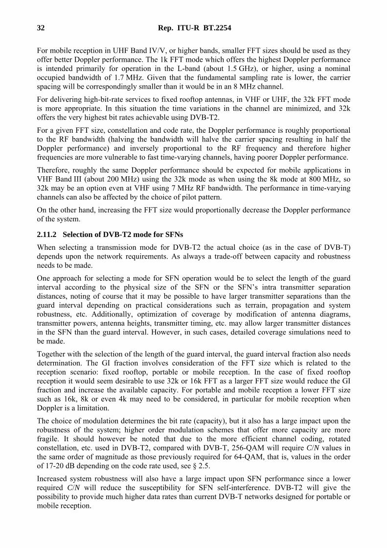
The results of choosing a certain FFT size are well known: an increased FFT size will give a greater delay tolerance for the same fractional guard interval, allowing larger SFNs to be constructed. Alternatively, a larger FFT size allows the same delay tolerance to be achieved with a smaller overhead due to the guard interval.
A larger FFT size implies a longer symbol duration, which means that the guard interval fraction is smaller for a given guard interval duration in time (see, for example, Fig. 2.12). This reduction in overhead leads to an increase in throughput ranging from 2.3% to 17.6%.
FIGURE 2.12
Guard interval overhead reduction with larger FFT size
20% overhead
~6% overhead
32 Rep. ITU-R BT.2254
For mobile reception in UHF Band IV/V, or higher bands, smaller FFT sizes should be used as they offer better Doppler performance. The 1k FFT mode which offers the highest Doppler performance is intended primarily for operation in the L-band (about 1.5 GHz), or higher, using a nominal occupied bandwidth of 1.7 MHz. Given that the fundamental sampling rate is lower, the carrier spacing will be correspondingly smaller than it would be in an 8 MHz channel.
For delivering high-bit-rate services to fixed rooftop antennas, in VHF or UHF, the 32k FFT mode is more appropriate. In this situation the time variations in the channel are minimized, and 32k offers the very highest bit rates achievable using DVB-T2.
For a given FFT size, constellation and code rate, the Doppler performance is roughly proportional to the RF bandwidth (halving the bandwidth will halve the carrier spacing resulting in half the Doppler performance) and inversely proportional to the RF frequency and therefore higher frequencies are more vulnerable to fast time-varying channels, having poorer Doppler performance.
Therefore, roughly the same Doppler performance should be expected for mobile applications in VHF Band III (about 200 MHz) using the 32k mode as when using the 8k mode at 800 MHz, so 32k may be an option even at VHF using 7 MHz RF bandwidth. The performance in time-varying channels can also be affected by the choice of pilot pattern.
On the other hand, increasing the FFT size would proportionally decrease the Doppler performance of the system.
2.11.2 Selection of DVB-T2 mode for SFNs
When selecting a transmission mode for DVB-T2 the actual choice (as in the case of DVB-T) depends upon the network requirements. As always a trade-off between capacity and robustness needs to be made.
One approach for selecting a mode for SFN operation would be to select the length of the guard interval according to the physical size of the SFN or the SFN’s intra transmitter separation distances, noting of course that it may be possible to have larger transmitter separations than the guard interval depending on practical considerations such as terrain, propagation and system robustness, etc. Additionally, optimization of coverage by modification of antenna diagrams, transmitter powers, antenna heights, transmitter timing, etc. may allow larger transmitter distances in the SFN than the guard interval. However, in such cases, detailed coverage simulations need to be made.
Together with the selection of the length of the guard interval, the guard interval fraction also needs determination. The GI fraction involves consideration of the FFT size which is related to the reception scenario: fixed rooftop, portable or mobile reception. In the case of fixed rooftop reception it would seem desirable to use 32k or 16k FFT as a larger FFT size would reduce the GI fraction and increase the available capacity. For portable and mobile reception a lower FFT size such as 16k, 8k or even 4k may need to be considered, in particular for mobile reception when Doppler is a limitation.
The choice of modulation determines the bit rate (capacity), but it also has a large impact upon the robustness of the system; higher order modulation schemes that offer more capacity are more fragile. It should however be noted that due to the more efficient channel coding, rotated constellation, etc. used in DVB-T2, compared with DVB-T, 256-QAM will require C/N values in the same order of magnitude as those previously required for 64-QAM, that is, values in the order of 17-20 dB depending on the code rate used, see § 2.5.
Increased system robustness will also have a large impact upon SFN performance since a lower required C/N will reduce the susceptibility for SFN self-interference. DVB-T2 will give the possibility to provide much higher data rates than current DVB-T networks designed for portable or mobile reception.

Rep. ITU-R BT.2254 33
Additionally, there are several Scattered Pilot Patterns (PP) available in DVB-T2, PP1 to PP8. They are described in more detail in § 2.7. The choice of pilot patterns will determine the performance for delayed signals arriving outside the guard interval as given by the Nyquist limit. Exceeding this Nyquist limit means that channel equalization is incorrect even if the fraction of inter-symbol interference (ISI) is small.
3 Receiver properties, sharing and compatibility, network planning parameters
For frequency and network planning of DVB-T2 knowledge of receiver properties, sharing and compatibility criteria and network planning parameters is required. Many of the network planning parameters and methods are well known from DVB-T and DVB-H planning. They comprise definition of coverage and reception modes, method of calculation of minimum median equivalent field strengths, treatment of antenna gain, feeder loss, man-made noise and building penetration loss, or the definition of location percentage requirements. All these are given in Annex 1.
In this section, aspects particular to DVB-T2 are described such as minimum receiver input levels, signal levels for planning, or protection ratios.
3.1 Minimum receiver signal input levels
To illustrate how the C/N ratio influences the minimum signal input level for the receiver, the latter has been calculated for five representative C/N ratios. They are given in Table 3.1. For other values simple linear interpolation can be applied.
The receiver noise figure has been chosen as 6 dB for the frequency Bands III, IV and V. Previously a number of different noise figure values ranging from 5-7 dB has been used. The EBU planning guideline for DVB-T [BPN005] suggests the value 7 dB. However, it is believed that improvements in digital receiver design will justify this small modification. Using the same receiver noise figure for all frequency bands will mean that the minimum receiver input signal level is independent of the transmitter frequency. If other noise figures are used in practice, the minimum receiver input signal level will change correspondingly by the same amount.
The minimum receiver input signal levels calculated here are used in § 3.3 to derive the minimum power flux-densities and corresponding minimum median equivalent field strength values for various frequency bands and reception modes.
Definitions:
B: Receiver noise bandwidth (Hz)
C/N: RF required by the system (dB)
F: Receiver noise figure (dB)
Pn: Receiver noise input power (dBW)
Ps min: Minimum receiver signal input power (dBW)
Us min: Minimum equivalent receiver input voltage into Zi (dBμV)
Zi: Receiver input impedance (75 Ω)
Constants:
k: Boltzmann’s Constant = 1.38*10–23 Ws/K
T0: Absolute temperature = 290 K
34 Rep. ITU-R BT.2254
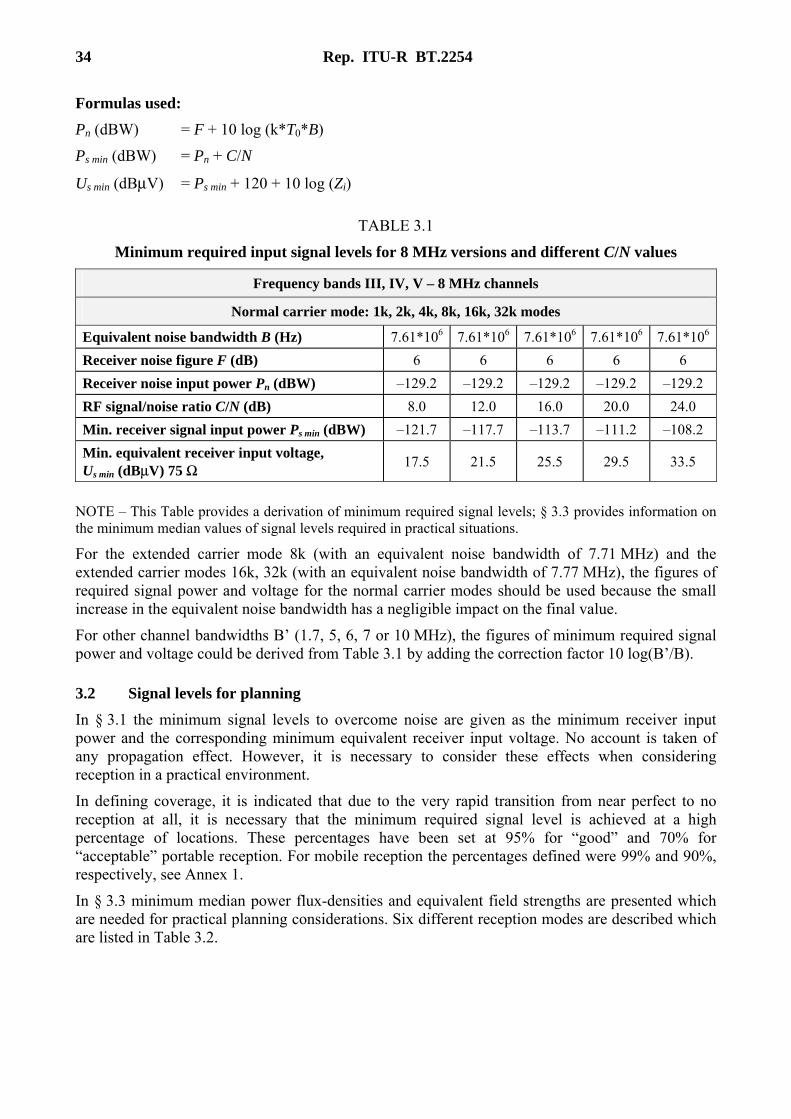
Formulas used:
Pn (dBW) = F + 10 log (k*T0*B)
Ps min (dBW) = Pn + C/N
Us min (dBμV) = Ps min + 120 + 10 log (Zi)
TABLE 3.1
Minimum required input signal levels for 8 MHz versions and different C/N values
Frequency bands III, IV, V – 8 MHz channels
Normal carrier mode: 1k, 2k, 4k, 8k, 16k, 32k modes
Equivalent noise bandwidth B (Hz) 7.61*106 7.61*106 7.61*106 7.61*106 7.61*106
Receiver noise figure F (dB) 6 6 6 6 6
Receiver noise input power Pn (dBW) –129.2 –129.2 –129.2 –129.2 –129.2
RF signal/noise ratio C/N (dB) 8.0 12.0 16.0 20.0 24.0
Min. receiver signal input power Ps min (dBW) –121.7 –117.7 –113.7 –111.2 –108.2
Min. equivalent receiver input voltage, Us min (dBμV) 75 Ω
17.5 21.5 25.5 29.5 33.5
NOTE – This Table provides a derivation of minimum required signal levels; § 3.3 provides information on the minimum median values of signal levels required in practical situations.
For the extended carrier mode 8k (with an equivalent noise bandwidth of 7.71 MHz) and the extended carrier modes 16k, 32k (with an equivalent noise bandwidth of 7.77 MHz), the figures of required signal power and voltage for the normal carrier modes should be used because the small increase in the equivalent noise bandwidth has a negligible impact on the final value.
For other channel bandwidths B’ (1.7, 5, 6, 7 or 10 MHz), the figures of minimum required signal power and voltage could be derived from Table 3.1 by adding the correction factor 10 log(B’/B).
3.2 Signal levels for planning
In § 3.1 the minimum signal levels to overcome noise are given as the minimum receiver input power and the corresponding minimum equivalent receiver input voltage. No account is taken of any propagation effect. However, it is necessary to consider these effects when considering reception in a practical environment.
In defining coverage, it is indicated that due to the very rapid transition from near perfect to no reception at all, it is necessary that the minimum required signal level is achieved at a high percentage of locations. These percentages have been set at 95% for “good” and 70% for “acceptable” portable reception. For mobile reception the percentages defined were 99% and 90%, respectively, see Annex 1.
In § 3.3 minimum median power flux-densities and equivalent field strengths are presented which are needed for practical planning considerations. Six different reception modes are described which are listed in Table 3.2.
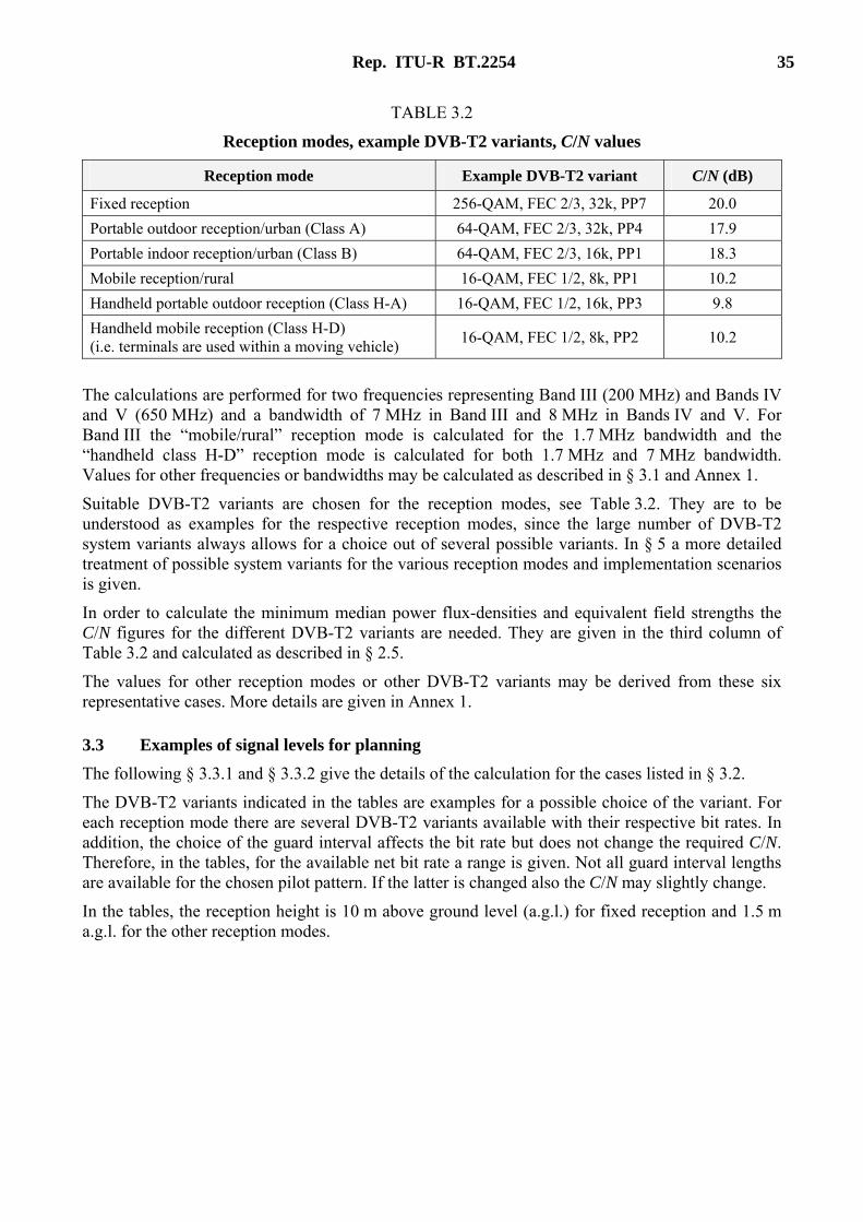
Rep. ITU-R BT.2254 35
TABLE 3.2
Reception modes, example DVB-T2 variants, C/N values
Reception mode Example DVB-T2 variant C/N (dB)
Fixed reception 256-QAM, FEC 2/3, 32k, PP7 20.0
Portable outdoor reception/urban (Class A) 64-QAM, FEC 2/3, 32k, PP4 17.9
Portable indoor reception/urban (Class B) 64-QAM, FEC 2/3, 16k, PP1 18.3
Mobile reception/rural 16-QAM, FEC 1/2, 8k, PP1 10.2
Handheld portable outdoor reception (Class H-A) 16-QAM, FEC 1/2, 16k, PP3 9.8
Handheld mobile reception (Class H-D) (i.e. terminals are used within a moving vehicle)
16-QAM, FEC 1/2, 8k, PP2 10.2
The calculations are performed for two frequencies representing Band III (200 MHz) and Bands IV and V (650 MHz) and a bandwidth of 7 MHz in Band III and 8 MHz in Bands IV and V. For Band III the “mobile/rural” reception mode is calculated for the 1.7 MHz bandwidth and the “handheld class H-D” reception mode is calculated for both 1.7 MHz and 7 MHz bandwidth. Values for other frequencies or bandwidths may be calculated as described in § 3.1 and Annex 1.
Suitable DVB-T2 variants are chosen for the reception modes, see Table 3.2. They are to be understood as examples for the respective reception modes, since the large number of DVB-T2 system variants always allows for a choice out of several possible variants. In § 5 a more detailed treatment of possible system variants for the various reception modes and implementation scenarios is given.
In order to calculate the minimum median power flux-densities and equivalent field strengths the C/N figures for the different DVB-T2 variants are needed. They are given in the third column of Table 3.2 and calculated as described in § 2.5.
The values for other reception modes or other DVB-T2 variants may be derived from these six representative cases. More details are given in Annex 1.
3.3 Examples of signal levels for planning
The following § 3.3.1 and § 3.3.2 give the details of the calculation for the cases listed in § 3.2.
The DVB-T2 variants indicated in the tables are examples for a possible choice of the variant. For each reception mode there are several DVB-T2 variants available with their respective bit rates. In addition, the choice of the guard interval affects the bit rate but does not change the required C/N. Therefore, in the tables, for the available net bit rate a range is given. Not all guard interval lengths are available for the chosen pilot pattern. If the latter is changed also the C/N may slightly change.
In the tables, the reception height is 10 m above ground level (a.g.l.) for fixed reception and 1.5 m a.g.l. for the other reception modes.

36 Rep. ITU-R BT.2254
3.3.1 DVB-T2 in Band III
Fixed Portable
outdoor/urban Portable
indoor/urban Mobile/rural
Handheld portable outdoor
Handheld mobile Class
H-D/ integrated antenna
Handheld mobile
Class H-D/ integrated antenna
Frequency Freq MHz 200 200 200 200 200 200 200
Minimum C/N required by system1
C/N dB 20.0 17.9 18.3 10.2 9.8 10.2 10.2
System variant (example)
256-QAM FEC 2/3, 32k,PP7 Normal
64-QAM FEC 2/3, 32k, PP4 Normal
64-QAM FEC 2/3, 16k,PP1 Normal
16-QAM FEC 1/2, 8k, PP1 Normal
16-QAM FEC 1/2, 16k,PP3 Normal
16-QAM FEC 1/2, 8k, PP2 Normal
16-QAM FEC 1/2, 8k, PP2 Normal
Bit rate (indicative values)
Mbit/s 30-35 22-25 19-24 2.2-2.8 10-13 2.2-2.8 10-12
Receiver noise figure F dB 6 6 6 6 6 6 6
Equivalent noise bandwidth
B MHz 6.66 6.66 6.66 1.54 6.66 1.54 6.66
Receiver noise input power
Pn dBW –128.6 –128.9 –128.5 –135.3 –132.2 –134.9 –128.5
Min. receiver signal input power
Ps min dBW –109.7 –111.8 –111.4 –125.9 –119.9 –125.9 –119.5
Min. equivalent receiver input voltage, 75 Ω
Umin dBµV 29.0 26.9 27.3 12.8 18.8 12.8 19.2
Feeder loss Lf dB 2 0 0 0 0 0 0
Antenna gain relative to half dipole
Gd dB 7 –2.2 –2.2 –2.2 –17 –17 –17
Effective antenna aperture
Aa dBm2 1.7 –7.5 –7.5 –7.5 –22.3 –22.3 –22.3
Min power flux-density at receiving location
θmin dB(W)/m2 –109.4 –104.3 –103.9 –118.4 –97.6 –103.6 –97.2
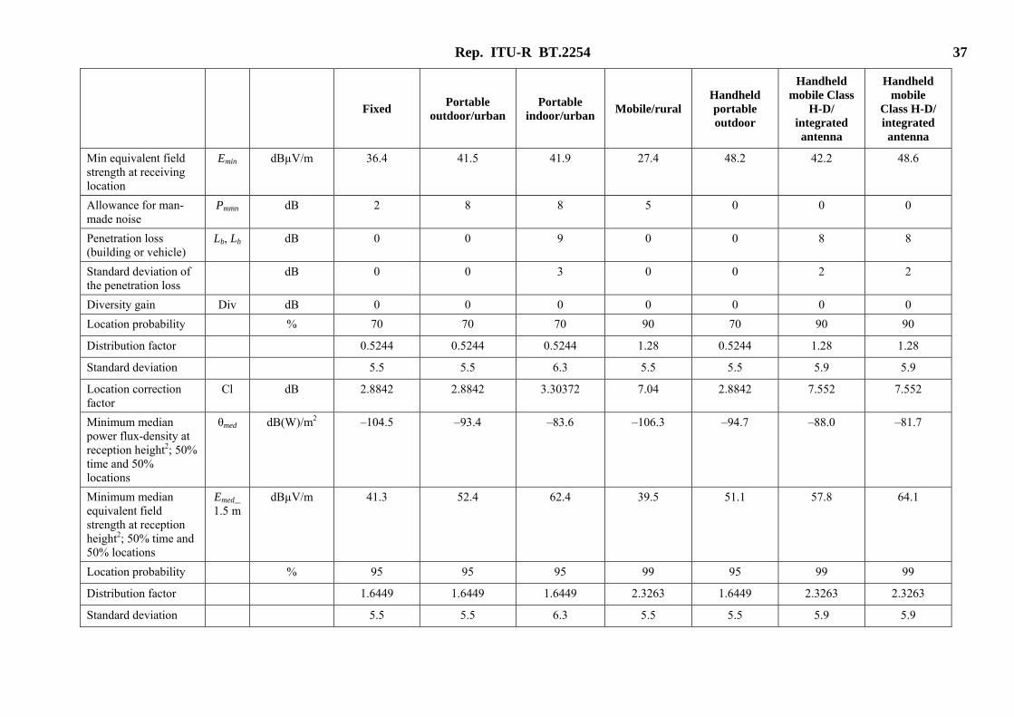
Rep. ITU-R BT.2254 37
Fixed Portable
outdoor/urban Portable
indoor/urban Mobile/rural
Handheld portable outdoor
Handheld mobile Class
H-D/ integrated antenna
Handheld mobile
Class H-D/ integrated antenna
Min equivalent field strength at receiving location
Emin dBµV/m 36.4 41.5 41.9 27.4 48.2 42.2 48.6
Allowance for man-made noise
Pmmn dB 2 8 8 5 0 0 0
Penetration loss (building or vehicle)
Lb, Lh dB 0 0 9 0 0 8 8
Standard deviation of the penetration loss
dB 0 0 3 0 0 2 2
Diversity gain Div dB 0 0 0 0 0 0 0
Location probability % 70 70 70 90 70 90 90
Distribution factor 0.5244 0.5244 0.5244 1.28 0.5244 1.28 1.28
Standard deviation 5.5 5.5 6.3 5.5 5.5 5.9 5.9
Location correction factor
Cl dB 2.8842 2.8842 3.30372 7.04 2.8842 7.552 7.552
Minimum median power flux-density at reception height2; 50% time and 50% locations
θmed dB(W)/m2 –104.5 –93.4 –83.6 –106.3 –94.7 –88.0 –81.7
Minimum median equivalent field strength at reception height2; 50% time and 50% locations
Emed_1.5 m
dBµV/m 41.3 52.4 62.4 39.5 51.1 57.8 64.1
Location probability % 95 95 95 99 95 99 99
Distribution factor 1.6449 1.6449 1.6449 2.3263 1.6449 2.3263 2.3263
Standard deviation 5.5 5.5 6.3 5.5 5.5 5.9 5.9
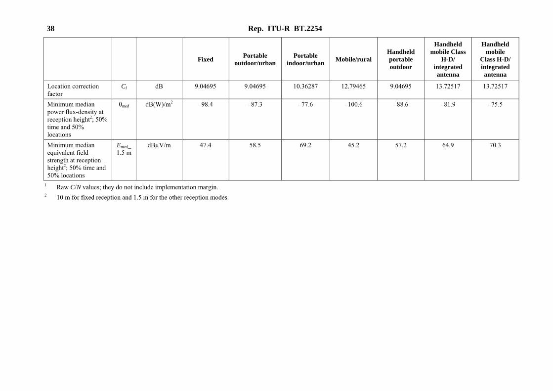
38 Rep. ITU-R BT.2254
Fixed Portable
outdoor/urban Portable
indoor/urban Mobile/rural
Handheld portable outdoor
Handheld mobile Class
H-D/ integrated antenna
Handheld mobile
Class H-D/ integrated antenna
Location correction factor
Cl dB 9.04695 9.04695 10.36287 12.79465 9.04695 13.72517 13.72517
Minimum median power flux-density at reception height2; 50% time and 50% locations
θmed dB(W)/m2 –98.4 –87.3 –77.6 –100.6 –88.6 –81.9 –75.5
Minimum median equivalent field strength at reception height2; 50% time and 50% locations
Emed_1.5 m
dBµV/m 47.4 58.5 69.2 45.2 57.2 64.9 70.3
1 Raw C/N values; they do not include implementation margin. 2 10 m for fixed reception and 1.5 m for the other reception modes.
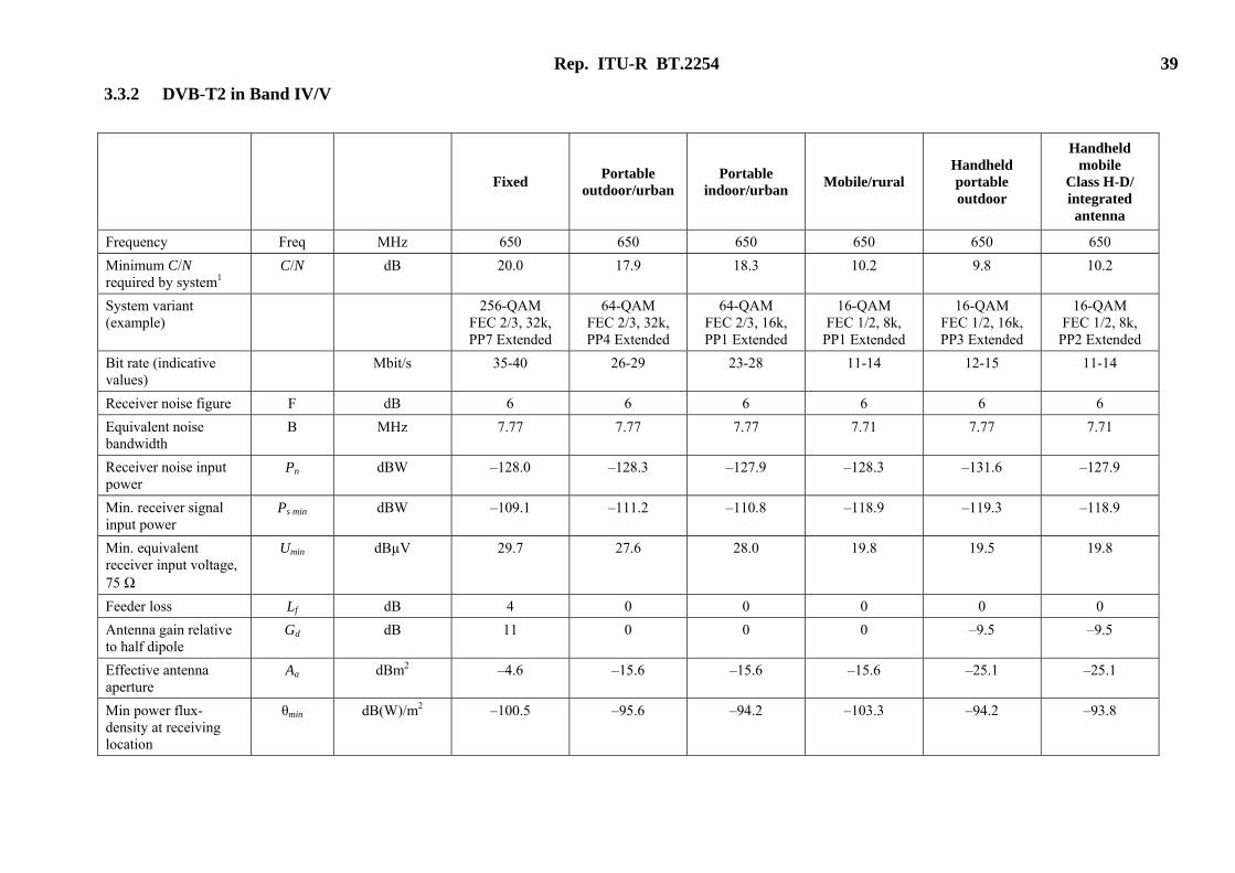
Rep. ITU-R BT.2254 39
3.3.2 DVB-T2 in Band IV/V
Fixed Portable
outdoor/urban Portable
indoor/urban Mobile/rural
Handheld portable outdoor
Handheld mobile
Class H-D/ integrated antenna
Frequency Freq MHz 650 650 650 650 650 650
Minimum C/N required by system1
C/N dB 20.0 17.9 18.3 10.2 9.8 10.2
System variant (example)
256-QAM FEC 2/3, 32k, PP7 Extended
64-QAM FEC 2/3, 32k, PP4 Extended
64-QAM FEC 2/3, 16k, PP1 Extended
16-QAM FEC 1/2, 8k,
PP1 Extended
16-QAM FEC 1/2, 16k, PP3 Extended
16-QAM FEC 1/2, 8k,
PP2 Extended
Bit rate (indicative values)
Mbit/s 35-40 26-29 23-28 11-14 12-15 11-14
Receiver noise figure F dB 6 6 6 6 6 6
Equivalent noise bandwidth
B MHz 7.77 7.77 7.77 7.71 7.77 7.71
Receiver noise input power
Pn dBW –128.0 –128.3 –127.9 –128.3 –131.6 –127.9
Min. receiver signal input power
Ps min dBW –109.1 –111.2 –110.8 –118.9 –119.3 –118.9
Min. equivalent receiver input voltage, 75 Ω
Umin dBµV 29.7 27.6 28.0 19.8 19.5 19.8
Feeder loss Lf dB 4 0 0 0 0 0
Antenna gain relative to half dipole
Gd dB 11 0 0 0 –9.5 –9.5
Effective antenna aperture
Aa dBm2 –4.6 –15.6 –15.6 –15.6 –25.1 –25.1
Min power flux-density at receiving location
θmin dB(W)/m2 –100.5 –95.6 –94.2 –103.3 –94.2 –93.8
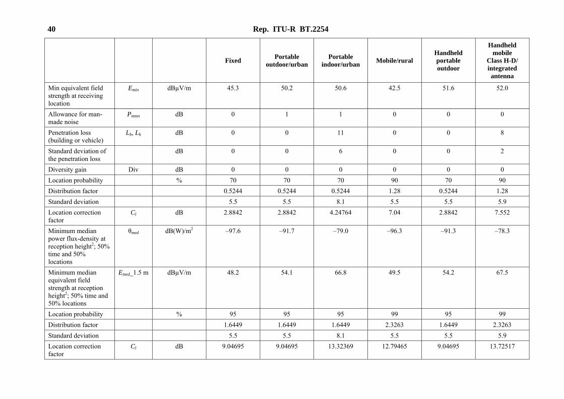
40 Rep. ITU-R BT.2254
Fixed Portable
outdoor/urban Portable
indoor/urban Mobile/rural
Handheld portable outdoor
Handheld mobile
Class H-D/ integrated antenna
Min equivalent field strength at receiving location
Emin dBµV/m 45.3 50.2 50.6 42.5 51.6 52.0
Allowance for man-made noise
Pmmn dB 0 1 1 0 0 0
Penetration loss (building or vehicle)
Lb, Lh dB 0 0 11 0 0 8
Standard deviation of the penetration loss
dB 0 0 6 0 0 2
Diversity gain Div dB 0 0 0 0 0 0
Location probability % 70 70 70 90 70 90
Distribution factor 0.5244 0.5244 0.5244 1.28 0.5244 1.28
Standard deviation 5.5 5.5 8.1 5.5 5.5 5.9
Location correction factor
Cl dB 2.8842 2.8842 4.24764 7.04 2.8842 7.552
Minimum median power flux-density at reception height2; 50% time and 50% locations
θmed dB(W)/m2 –97.6 –91.7 –79.0 –96.3 –91.3 –78.3
Minimum median equivalent field strength at reception height2; 50% time and 50% locations
Emed_1.5 m dBµV/m 48.2 54.1 66.8 49.5 54.2 67.5
Location probability % 95 95 95 99 95 99
Distribution factor 1.6449 1.6449 1.6449 2.3263 1.6449 2.3263
Standard deviation 5.5 5.5 8.1 5.5 5.5 5.9
Location correction factor
Cl dB 9.04695 9.04695 13.32369 12.79465 9.04695 13.72517
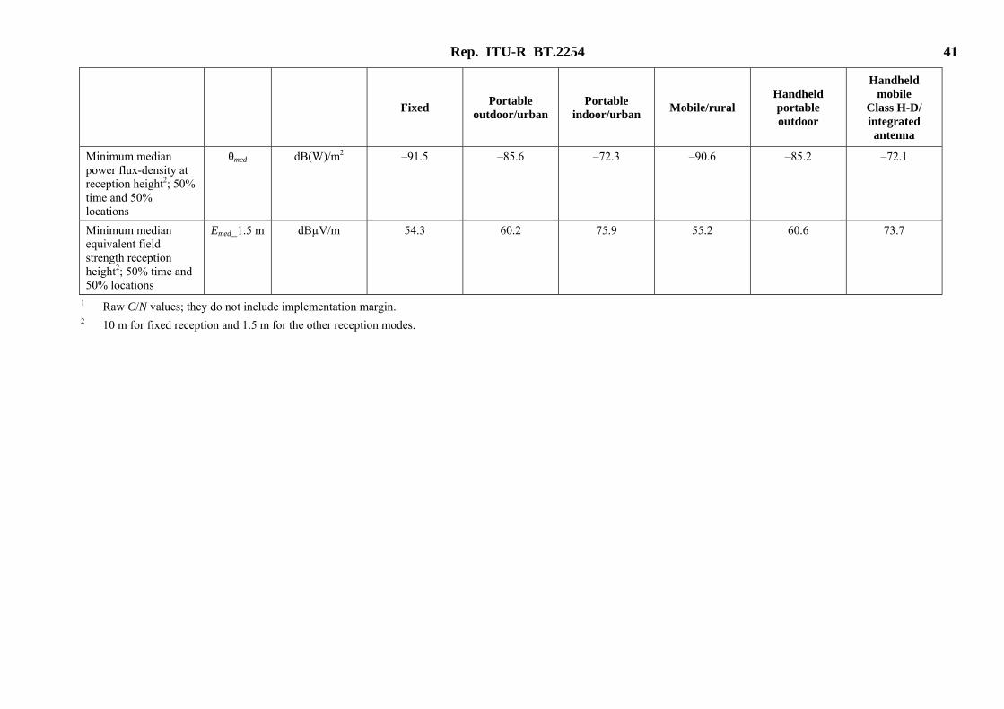
Rep. ITU-R BT.2254 41
Fixed Portable
outdoor/urban Portable
indoor/urban Mobile/rural
Handheld portable outdoor
Handheld mobile
Class H-D/ integrated antenna
Minimum median power flux-density at reception height2; 50% time and 50% locations
θmed dB(W)/m2 –91.5 –85.6 –72.3 –90.6 –85.2 –72.1
Minimum median equivalent field strength reception height2; 50% time and 50% locations
Emed_1.5 m dBµV/m 54.3 60.2 75.9 55.2 60.6 73.7
1 Raw C/N values; they do not include implementation margin. 2 10 m for fixed reception and 1.5 m for the other reception modes.
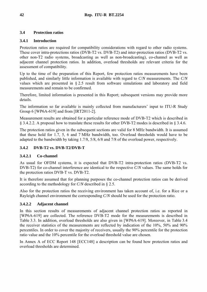
42 Rep. ITU-R BT.2254
3.4 Protection ratios
3.4.1 Introduction
Protection ratios are required for compatibility considerations with regard to other radio systems. These cover intra-protections ratios (DVB-T2 vs. DVB-T2) and inter-protection ratios (DVB-T2 vs. other non-T2 radio systems, broadcasting as well as non-broadcasting), co-channel as well as adjacent channel protection ratios. In addition, overload thresholds are relevant criteria for the assessment of compatibility.
Up to the time of the preparation of this Report, few protection ratios measurements have been published, and similarly little information is available with regard to C/N measurements. The C/N values which are presented in § 2.5 result from software simulations and laboratory and field measurements and remain to be confirmed.
Therefore, limited information is presented in this Report; subsequent versions may provide more details.
The information so far available is mainly collected from manufacturers’ input to ITU-R Study Group 6 [WP6A-619] and from [IRT2011-2].
Measurement results are obtained for a particular reference mode of DVB-T2 which is described in § 3.4.2.2. A proposal how to translate these results for other DVB-T2 modes is described in § 3.4.6.
The protection ratios given in the subsequent sections are valid for 8 MHz bandwidth. It is assumed that these hold for 1.7, 5, 6 and 7 MHz bandwidth, too. Overload thresholds would have to be adapted to the bandwidth by taking 1.7/8, 5/8, 6/8 and 7/8 of the overload power, respectively.
3.4.2 DVB-T2 vs. DVB-T2/DVB-T
3.4.2.1 Co-channel
As usual for OFDM systems, it is expected that DVB-T2 intra-protection ratios (DVB-T2 vs. DVB-T2) for co-channel interference are identical to the respective C/N values. The same holds for the protection ratios DVB-T vs. DVB-T2.
It is therefore assumed that for planning purposes the co-channel protection ratios can be derived according to the methodology for C/N described in § 2.5.
Also for the protection ratios the receiving environment has taken account of, i.e. for a Rice or a Rayleigh channel environment the corresponding C/N should be used for the protection ratio.
3.4.2.2 Adjacent channel
In this section results of measurements of adjacent channel protection ratios as reported in [WP6A-619] are collected. The reference DVB-T2 mode for the measurements is described in Table 3.3. In addition, overload thresholds are also given in [WP6A-619]. Moreover, in Table 3.4 the receiver statistics of the measurements are reflected by indication of the 10%, 50% and 90% percentiles. In order to cover the majority of receivers, usually the 90% percentile for the protection ratio value and the 10% percentile for the overload threshold value are chosen.
In Annex A of ECC Report 148 [ECC148] a description can be found how protection ratios and overload thresholds are determined.
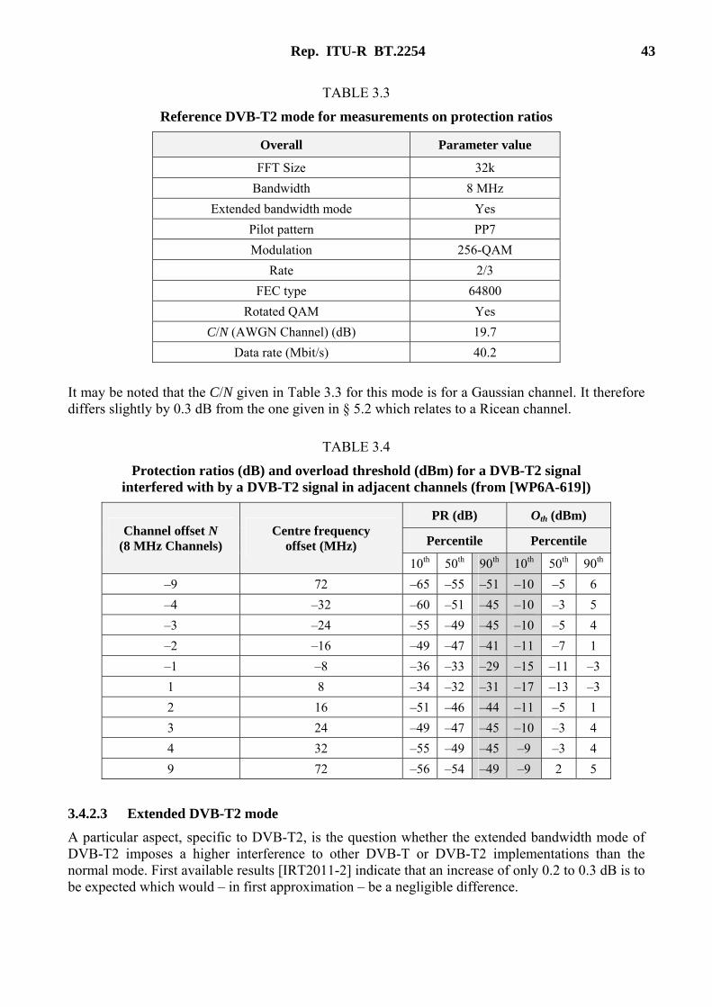
Rep. ITU-R BT.2254 43
TABLE 3.3
Reference DVB-T2 mode for measurements on protection ratios
Overall Parameter value
FFT Size 32k
Bandwidth 8 MHz
Extended bandwidth mode Yes
Pilot pattern PP7
Modulation 256-QAM
Rate 2/3
FEC type 64800
Rotated QAM Yes
C/N (AWGN Channel) (dB) 19.7
Data rate (Mbit/s) 40.2
It may be noted that the C/N given in Table 3.3 for this mode is for a Gaussian channel. It therefore differs slightly by 0.3 dB from the one given in § 5.2 which relates to a Ricean channel.
TABLE 3.4
Protection ratios (dB) and overload threshold (dBm) for a DVB-T2 signal interfered with by a DVB-T2 signal in adjacent channels (from [WP6A-619])
Channel offset N (8 MHz Channels)
Centre frequency offset (MHz)
PR (dB) Oth (dBm)
Percentile Percentile
10th 50th 90th 10th 50th 90th
–9 72 –65 –55 –51 –10 –5 6
–4 –32 –60 –51 –45 –10 –3 5
–3 –24 –55 –49 –45 –10 –5 4
–2 –16 –49 –47 –41 –11 –7 1
–1 –8 –36 –33 –29 –15 –11 –3
1 8 –34 –32 –31 –17 –13 –3
2 16 –51 –46 –44 –11 –5 1
3 24 –49 –47 –45 –10 –3 4
4 32 –55 –49 –45 –9 –3 4
9 72 –56 –54 –49 –9 2 5
3.4.2.3 Extended DVB-T2 mode
A particular aspect, specific to DVB-T2, is the question whether the extended bandwidth mode of DVB-T2 imposes a higher interference to other DVB-T or DVB-T2 implementations than the normal mode. First available results [IRT2011-2] indicate that an increase of only 0.2 to 0.3 dB is to be expected which would – in first approximation – be a negligible difference.

44 Rep. ITU-R BT.2254
3.4.3 DVB-T2 vs. T-DAB
No information is available yet on protection ratios for DVB-T2 interfered with by T-DAB.
For the protection ratios of T-DAB interfered with by DVB-T2 it is assumed that the same values hold as they are reported for the interference by DVB-T. These can be found, e.g. in [RRC06].
3.4.4 DVB-T2 vs. Analogue TV
No information is available yet on protection ratios for DVB-T2 interfered with by Analogue TV.
For the protection ratios of Analogue TV interfered with by DVB-T2 it is assumed that the same values hold as they are reported for the interference by DVB-T. These can be found, e.g. in [RRC06].
3.4.5 DVB-T2 vs. LTE
From the large class of cases of interference of DVB-T2 with other (non-broadcasting) services the case of LTE is the most relevant one since close adjacent channel appearance in the UHF band is possible and even co-channel relationship may be relevant.
3.4.5.1 Co-channel
No information is available yet.
3.4.5.2 Adjacent channel
The case of adjacent channel interference of DVB-T2 by LTE was studied in the context of the discussion of the digital dividend in Europe [ECC148]. The following tables show protection ratios and overload thresholds for three different traffic loadings on the LTE base station. Low traffic loadings increase the time variation in the LTE interference signal which causes degradations in protection ratios and overload thresholds in some receiver designs. Again, the information is taken from [WP6A-619] and the same reference mode of DVB-T2 is used as in § 3.4.2.2.
It should be noted that these values are preliminary since they were derived from a limited number of measurements and therefore further measurement is needed to finalize the work.
Table 3.5 gives the information for DVB-T2 interfered with by an LTE base station (BS). Values for interference by an LTE terminal (User Equipment: UE) are given in Table 3.6.
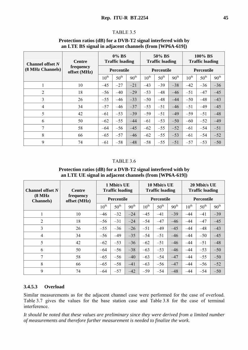
Rep. ITU-R BT.2254 45
TABLE 3.5
Protection ratios (dB) for a DVB-T2 signal interfered with by an LTE BS signal in adjacent channels (from [WP6A-619])
Channel offset N (8 MHz Channels)
Centre frequency
offset (MHz)
0% BS Traffic loading
50% BS Traffic loading
100% BS Traffic loading
Percentile Percentile Percentile
10th 50th 90th 10th 50th 90th 10th 50th 90th
1 10 –45 –27 –21 –43 –39 –38 –42 –36 –36
2 18 –56 –40 –29 –53 –48 –46 –51 –47 –45
3 26 –55 –46 –33 –50 –48 –44 –50 –48 –43
4 34 –57 –46 –37 –53 –51 –46 –51 –49 –45
5 42 –61 –53 –39 –59 –51 –49 –59 –51 –48
6 50 –62 –55 –44 –61 –53 –50 –60 –52 –49
7 58 –64 –56 –45 –62 –55 –52 –61 –54 –51
8 66 –65 –57 –46 –62 –55 –53 –61 –54 –52
9 74 –61 –58 –48 –58 –55 –51 –57 –53 –50
TABLE 3.6
Protection ratios (dB) for a DVB-T2 signal interfered with by an LTE UE signal in adjacent channels (from [WP6A-619])
Channel offset N (8 MHz
Channels)
Centre frequency
offset (MHz)
1 Mbit/s UE Traffic loading
10 Mbit/s UE Traffic loading
20 Mbit/s UE Traffic loading
Percentile Percentile Percentile
10th 50th 90th 10th 50th 90th 10th 50th 90th
1 10 –46 –32 –24 –45 –41 –39 –44 –41 –39
2 18 –56 –31 –24 –54 –47 –46 –44 –47 –45
3 26 –55 –36 –26 –51 –49 –45 –44 –48 –43
4 34 –56 –49 –35 –54 –51 –46 –44 –50 –45
5 42 –62 –53 –36 –62 –51 –46 –44 –51 –48
6 50 –64 –56 –38 –63 –53 –46 –44 –53 –50
7 58 –65 –56 –40 –63 –54 –47 –44 –55 –50
8 66 –65 –58 –41 –63 –56 –47 –44 –56 –52
9 74 –64 –57 –42 –59 –54 –48 –44 –54 –50
3.4.5.3 Overload
Similar measurements as for the adjacent channel case were performed for the case of overload. Table 3.7 gives the values for the base station case and Table 3.8 for the case of terminal interference.
It should be noted that these values are preliminary since they were derived from a limited number of measurements and therefore further measurement is needed to finalize the work.

46 Rep. ITU-R BT.2254
TABLE 3.7
Overload thresholds (dBm) for a DVB-T2 signal interfered with by an LTE BS signal in adjacent channels (from [WP6A-619])
Channel offset N (8 MHz
Channels)
Centre frequency offset (MHz)
0% BS Traffic loading
50% BS Traffic loading
100% BS Traffic loading
Oth (dBm) Oth (dBm) Oth (dBm)
10th 50th 90th 10th 50th 90th 10th 50th 90th
1 10 –23 –12 –5 –14 –7 0 –15 –8 0
2 18 –16 0 5 –9 –2 2 –9 –3 1
3 26 –16 –1 8 –9 –2 5 –8 –3 4
4 34 –15 1 9 –13 –2 6 –8 –2 5
5 42 –16 4 9 –8 2 6 –8 2 5
6 50 –16 5 10 –8 5 6 –8 4 5
7 58 –16 5 10 –7 1 7 –8 5 6
8 66 –17 5 10 –8 1 6 –8 4 5
9 74 –16 5 10 –8 5 6 –8 4 5
TABLE 3.8
Overload thresholds (dBm) for a DVB-T2 signal interfered with by an LTE UE signal in adjacent channels (from [WP6A-619])
Channel offset N (8 MHz Channels)
Centre frequency offset (MHz)
0% BS Traffic loading
50% BS Traffic loading
100% BS Traffic loading
Oth (dBm) Oth (dBm) Oth (dBm)
10th 50th 90th 10th 50th 90th 10th 50th 90th
1 10 –38 –6 –1 –10 –7 1 –13 –6 2
2 18 –18 4 9 –7 –2 5 –8 –2 4
3 26 –20 1 9 –7 –1 6 –7 –2 5
4 34 –28 2 9 –13 –3 6 –14 –2 5
5 42 –19 6 9 –7 1 6 –7 2 6
6 50 –18 8 10 –7 4 7 –7 4 6
7 58 –16 8 10 –7 4 7 –7 4 7
8 66 –16 8 11 –7 0 8 –7 4 7
9 74 –17 8 11 –7 4 7 –7 4 7
3.4.6 Protection ratios for DVB-T2 modes other than the reference mode
The following method is proposed to adapt the above given protection ratios to DVB-T2 modes other than the reference mode described in § 3.4.2.2. This approach is to be regarded as a rough approximation. Additional measurements for other DVB-T2 modes would be desirable.
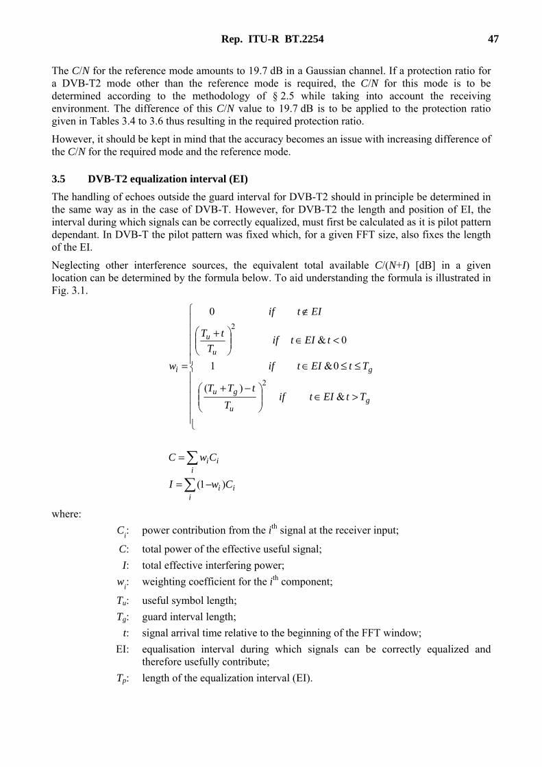
Rep. ITU-R BT.2254 47
The C/N for the reference mode amounts to 19.7 dB in a Gaussian channel. If a protection ratio for a DVB-T2 mode other than the reference mode is required, the C/N for this mode is to be determined according to the methodology of § 2.5 while taking into account the receiving environment. The difference of this C/N value to 19.7 dB is to be applied to the protection ratio given in Tables 3.4 to 3.6 thus resulting in the required protection ratio.
However, it should be kept in mind that the accuracy becomes an issue with increasing difference of the C/N for the required mode and the reference mode.
3.5 DVB-T2 equalization interval (EI)
The handling of echoes outside the guard interval for DVB-T2 should in principle be determined in the same way as in the case of DVB-T. However, for DVB-T2 the length and position of EI, the interval during which signals can be correctly equalized, must first be calculated as it is pilot pattern dependant. In DVB-T the pilot pattern was fixed which, for a given FFT size, also fixes the length of the EI.
Neglecting other interference sources, the equivalent total available C/(N+I) [dB] in a given location can be determined by the formula below. To aid understanding the formula is illustrated in Fig. 3.1.
iii
iii
gu
gu
g
u
u
i
CwI
CwC
TtEItifT
tTT
TtEItif
tEItifT
tT
EItif
w
)1(
& )(
0& 1
0&
0
2
2
−=
=
>∈
−+
≤≤∈
<∈
+
∉
=
where:
Ci: power contribution from the ith signal at the receiver input;
C: total power of the effective useful signal;
I: total effective interfering power;
wi: weighting coefficient for the ith component;
Tu: useful symbol length;
Tg: guard interval length;
t: signal arrival time relative to the beginning of the FFT window;
EI: equalisation interval during which signals can be correctly equalized and therefore usefully contribute;
Tp: length of the equalization interval (EI).
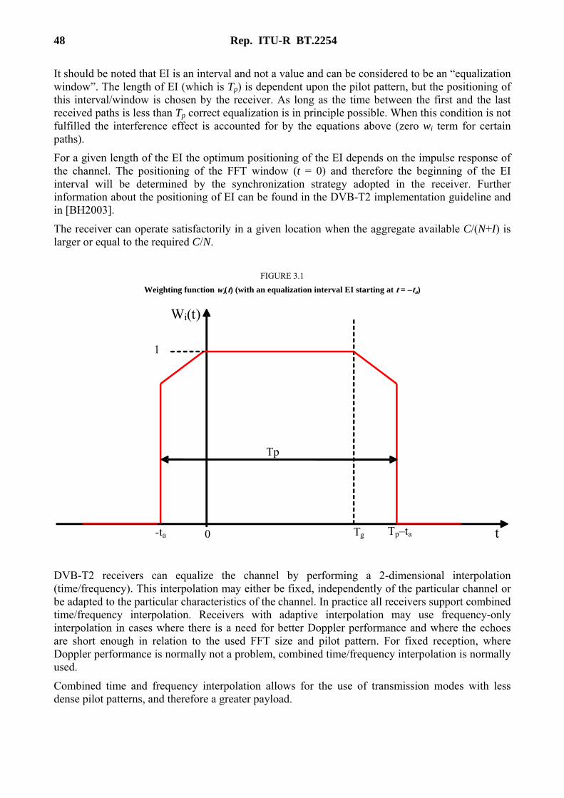
48 Rep. ITU-R BT.2254
It should be noted that EI is an interval and not a value and can be considered to be an “equalization window”. The length of EI (which is Tp) is dependent upon the pilot pattern, but the positioning of this interval/window is chosen by the receiver. As long as the time between the first and the last received paths is less than Tp correct equalization is in principle possible. When this condition is not fulfilled the interference effect is accounted for by the equations above (zero wi term for certain paths).
For a given length of the EI the optimum positioning of the EI depends on the impulse response of the channel. The positioning of the FFT window (t = 0) and therefore the beginning of the EI interval will be determined by the synchronization strategy adopted in the receiver. Further information about the positioning of EI can be found in the DVB-T2 implementation guideline and in [BH2003].
The receiver can operate satisfactorily in a given location when the aggregate available C/(N+I) is larger or equal to the required C/N.
FIGURE 3.1
Weighting function wi(t) (with an equalization interval EI starting at t = –ta)
DVB-T2 receivers can equalize the channel by performing a 2-dimensional interpolation (time/frequency). This interpolation may either be fixed, independently of the particular channel or be adapted to the particular characteristics of the channel. In practice all receivers support combined time/frequency interpolation. Receivers with adaptive interpolation may use frequency-only interpolation in cases where there is a need for better Doppler performance and where the echoes are short enough in relation to the used FFT size and pilot pattern. For fixed reception, where Doppler performance is normally not a problem, combined time/frequency interpolation is normally used.
Combined time and frequency interpolation allows for the use of transmission modes with less dense pilot patterns, and therefore a greater payload.
Tp
t0 Tg Tp–ta-ta
1
Wi(t)
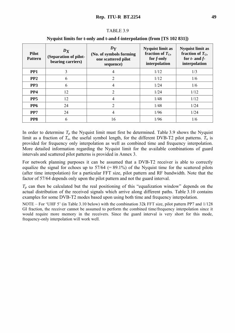
Rep. ITU-R BT.2254 49
TABLE 3.9
Nyquist limits for t-only and t-and-f-interpolation (from [TS 102 831])
Pilot Pattern
DX
(Separation of pilot-bearing carriers)
DY (No. of symbols forming
one scattered pilot sequence)
Nyquist limit as fraction of TU,
for f-only interpolation
Nyquist limit as fraction of TU,
for t- and f-interpolation
PP1 3 4 1/12 1/3
PP2 6 2 1/12 1/6
PP3 6 4 1/24 1/6
PP4 12 2 1/24 1/12
PP5 12 4 1/48 1/12
PP6 24 2 1/48 1/24
PP7 24 4 1/96 1/24
PP8 6 16 1/96 1/6
In order to determine Tp the Nyquist limit must first be determined. Table 3.9 shows the Nyquist limit as a fraction of Tu, the useful symbol length, for the different DVB-T2 pilot patterns. Tu is provided for frequency only interpolation as well as combined time and frequency interpolation. More detailed information regarding the Nyquist limit for the available combinations of guard intervals and scattered pilot patterns is provided in Annex 3.
For network planning purposes it can be assumed that a DVB-T2 receiver is able to correctly equalize the signal for echoes up to 57/64 (= 89.1%) of the Nyquist time for the scattered pilots (after time interpolation) for a particular FFT size, pilot pattern and RF bandwidth. Note that the factor of 57/64 depends only upon the pilot pattern and not the guard interval.
Tp can then be calculated but the real positioning of this “equalization window” depends on the actual distribution of the received signals which arrive along different paths. Table 3.10 contains examples for some DVB-T2 modes based upon using both time and frequency interpolation.
NOTE – For ‘UHF 5’ (in Table 3.10 below) with the combination 32k FFT size, pilot pattern PP7 and 1/128 GI fraction, the receiver cannot be assumed to perform the combined time/frequency interpolation since it would require more memory in the receivers. Since the guard interval is very short for this mode, frequency-only interpolation will work well.
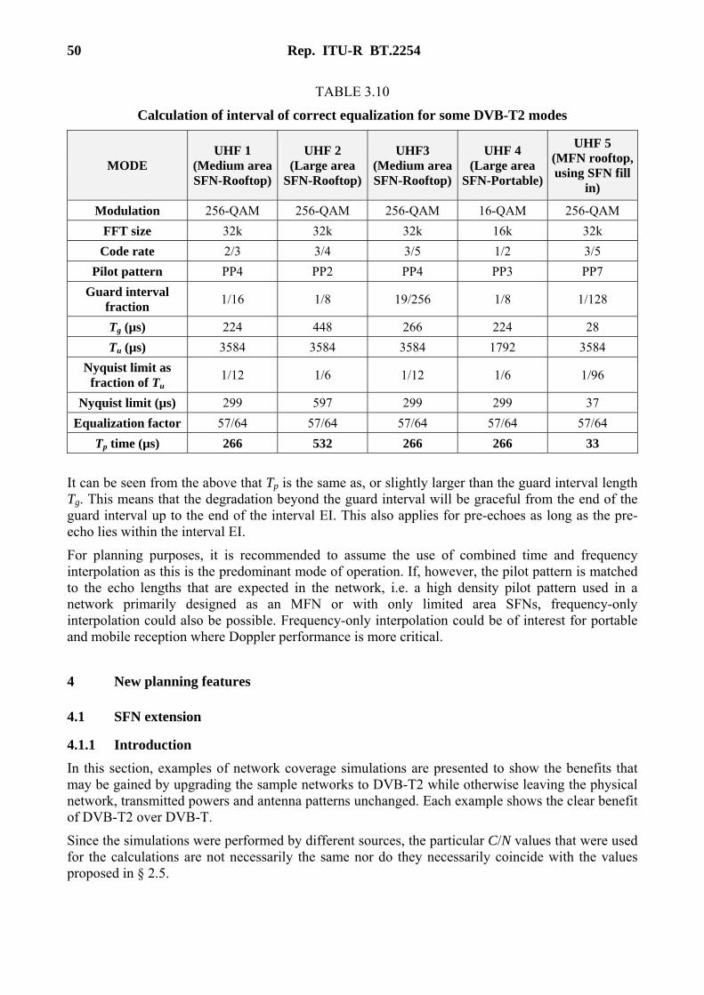
50 Rep. ITU-R BT.2254
TABLE 3.10
Calculation of interval of correct equalization for some DVB-T2 modes
MODE UHF 1
(Medium area SFN-Rooftop)
UHF 2 (Large area
SFN-Rooftop)
UHF3 (Medium areaSFN-Rooftop)
UHF 4 (Large area
SFN-Portable)
UHF 5 (MFN rooftop,using SFN fill
in)
Modulation 256-QAM 256-QAM 256-QAM 16-QAM 256-QAM
FFT size 32k 32k 32k 16k 32k
Code rate 2/3 3/4 3/5 1/2 3/5
Pilot pattern PP4 PP2 PP4 PP3 PP7
Guard interval fraction
1/16 1/8 19/256 1/8 1/128
Tg (µs) 224 448 266 224 28
Tu (µs) 3584 3584 3584 1792 3584
Nyquist limit as fraction of Tu
1/12 1/6 1/12 1/6 1/96
Nyquist limit (µs) 299 597 299 299 37
Equalization factor 57/64 57/64 57/64 57/64 57/64
Tp time (µs) 266 532 266 266 33
It can be seen from the above that Tp is the same as, or slightly larger than the guard interval length Tg. This means that the degradation beyond the guard interval will be graceful from the end of the guard interval up to the end of the interval EI. This also applies for pre-echoes as long as the pre-echo lies within the interval EI.
For planning purposes, it is recommended to assume the use of combined time and frequency interpolation as this is the predominant mode of operation. If, however, the pilot pattern is matched to the echo lengths that are expected in the network, i.e. a high density pilot pattern used in a network primarily designed as an MFN or with only limited area SFNs, frequency-only interpolation could also be possible. Frequency-only interpolation could be of interest for portable and mobile reception where Doppler performance is more critical.
4 New planning features
4.1 SFN extension
4.1.1 Introduction
In this section, examples of network coverage simulations are presented to show the benefits that may be gained by upgrading the sample networks to DVB-T2 while otherwise leaving the physical network, transmitted powers and antenna patterns unchanged. Each example shows the clear benefit of DVB-T2 over DVB-T.
Since the simulations were performed by different sources, the particular C/N values that were used for the calculations are not necessarily the same nor do they necessarily coincide with the values proposed in § 2.5.
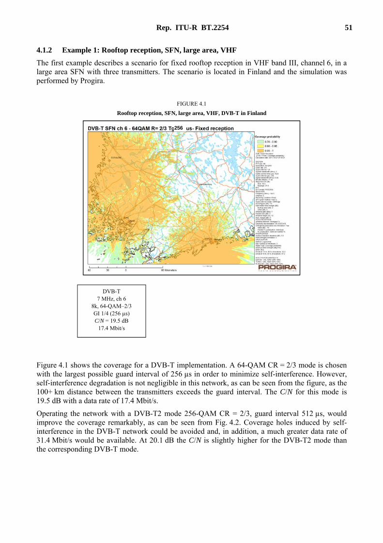
Rep. ITU-R BT.2254 51
4.1.2 Example 1: Rooftop reception, SFN, large area, VHF
The first example describes a scenario for fixed rooftop reception in VHF band III, channel 6, in a large area SFN with three transmitters. The scenario is located in Finland and the simulation was performed by Progira.
FIGURE 4.1
Rooftop reception, SFN, large area, VHF, DVB-T in Finland
Figure 4.1 shows the coverage for a DVB-T implementation. A 64-QAM CR = 2/3 mode is chosen with the largest possible guard interval of 256 µs in order to minimize self-interference. However, self-interference degradation is not negligible in this network, as can be seen from the figure, as the 100+ km distance between the transmitters exceeds the guard interval. The C/N for this mode is 19.5 dB with a data rate of 17.4 Mbit/s.
Operating the network with a DVB-T2 mode 256-QAM CR = 2/3, guard interval 512 µs, would improve the coverage remarkably, as can be seen from Fig. 4.2. Coverage holes induced by self-interference in the DVB-T network could be avoided and, in addition, a much greater data rate of 31.4 Mbit/s would be available. At 20.1 dB the C/N is slightly higher for the DVB-T2 mode than the corresponding DVB-T mode.
256
DVB-T 7 MHz, ch 6
8k, 64-QAM–2/3 GI 1/4 (256 µs) C/N = 19.5 dB
17.4 Mbit/s
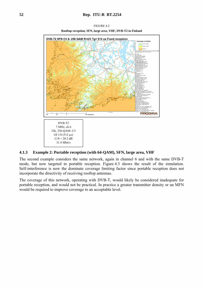
52 Rep. ITU-R BT.2254
FIGURE 4.2
Rooftop reception, SFN, large area, VHF, DVB-T2 in Finland
4.1.3 Example 2: Portable reception (with 64-QAM), SFN, large area, VHF
The second example considers the same network, again in channel 6 and with the same DVB-T mode, but now targeted to portable reception. Figure 4.3 shows the result of the simulation. Self-interference is now the dominate coverage limiting factor since portable reception does not incorporate the directivity of receiving rooftop antennas.
The coverage of this network, operating with DVB-T, would likely be considered inadequate for portable reception, and would not be practical. In practice a greater transmitter density or an MFN would be required to improve coverage to an acceptable level.
DVB-T2 7 MHz, ch 6
32k, 256-QAM–2/3 GI 1/8 (512 µs) C/N = 20.2 dB
31.4 Mbit/s
Rep. ITU-R BT.2254 53
FIGURE 4.3
Portable reception, SFN, large area, VHF, DVB-T in Finland
The situation would be markedly improved for a DVB-T2 implementation where a longer guard interval could avoid the deleterious self-interference effects. In Fig. 4.4 the DVB-T2 mode 64-QAM CR = 3/5 has been modelled, providing a similar data rate to the DVB-T mode above. Now large areas are covered and the sparse transmitter network may prove viable.
DVB-T 7 MHz, ch 6
8k, 64-QAM–2/3 GI 1/4 (256 µs) C/N = 21.8 dB
19.9 Mbit/s
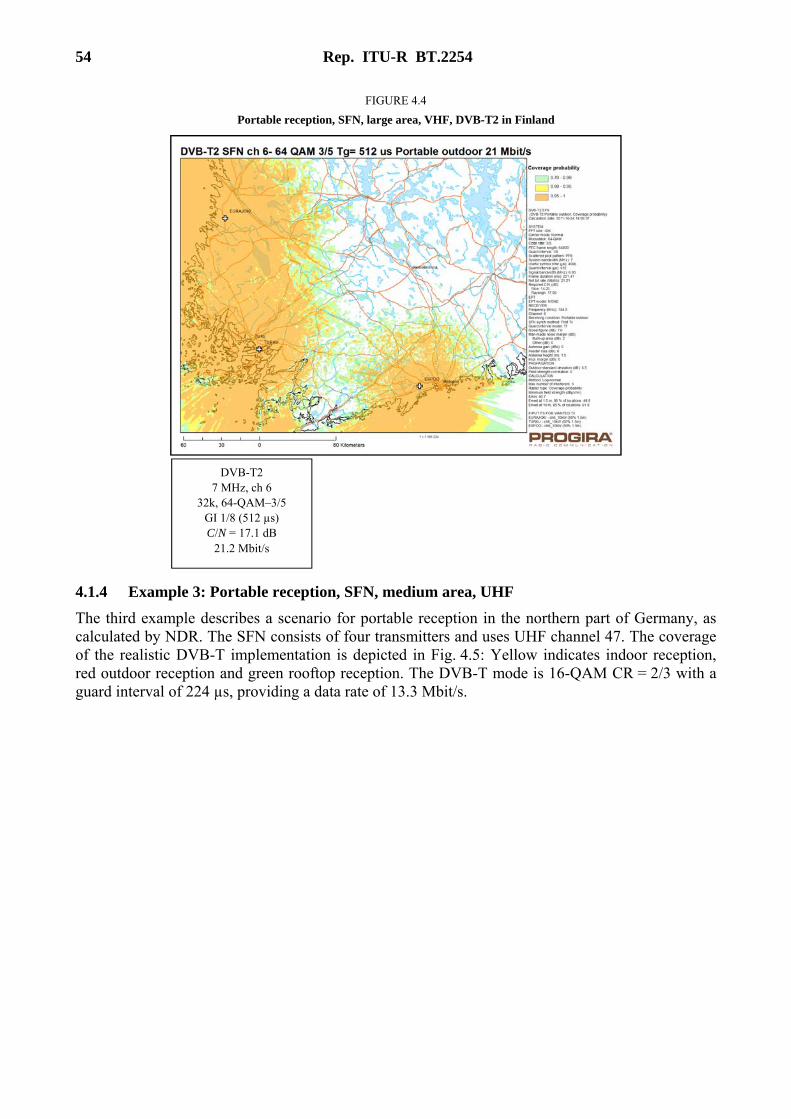
54 Rep. ITU-R BT.2254
FIGURE 4.4
Portable reception, SFN, large area, VHF, DVB-T2 in Finland
4.1.4 Example 3: Portable reception, SFN, medium area, UHF
The third example describes a scenario for portable reception in the northern part of Germany, as calculated by NDR. The SFN consists of four transmitters and uses UHF channel 47. The coverage of the realistic DVB-T implementation is depicted in Fig. 4.5: Yellow indicates indoor reception, red outdoor reception and green rooftop reception. The DVB-T mode is 16-QAM CR = 2/3 with a guard interval of 224 µs, providing a data rate of 13.3 Mbit/s.
DVB-T2 7 MHz, ch 6
32k, 64-QAM–3/5 GI 1/8 (512 µs) C/N = 17.1 dB
21.2 Mbit/s
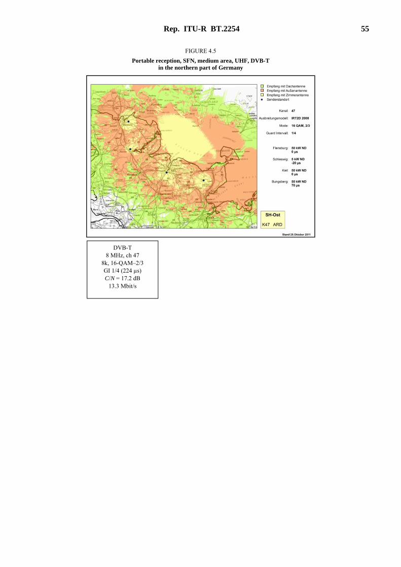
Rep. ITU-R BT.2254 55
FIGURE 4.5
Portable reception, SFN, medium area, UHF, DVB-T in the northern part of Germany
DVB-T 8 MHz, ch 47
8k, 16-QAM–2/3 GI 1/4 (224 µs) C/N = 17.2 dB
13.3 Mbit/s
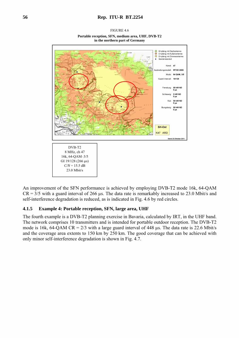
56 Rep. ITU-R BT.2254
FIGURE 4.6
Portable reception, SFN, medium area, UHF, DVB-T2 in the northern part of Germany
An improvement of the SFN performance is achieved by employing DVB-T2 mode 16k, 64-QAM CR = 3/5 with a guard interval of 266 µs. The data rate is remarkably increased to 23.0 Mbit/s and self-interference degradation is reduced, as is indicated in Fig. 4.6 by red circles.
4.1.5 Example 4: Portable reception, SFN, large area, UHF
The fourth example is a DVB-T2 planning exercise in Bavaria, calculated by IRT, in the UHF band. The network comprises 10 transmitters and is intended for portable outdoor reception. The DVB-T2 mode is 16k, 64-QAM CR = 2/3 with a large guard interval of 448 µs. The data rate is 22.6 Mbit/s and the coverage area extents to 150 km by 250 km. The good coverage that can be achieved with only minor self-interference degradation is shown in Fig. 4.7.
DVB-T2 8 MHz, ch 47
16k, 64-QAM–3/5 GI 19/128 (266 µs)
C/N = 15.5 dB 23.0 Mbit/s
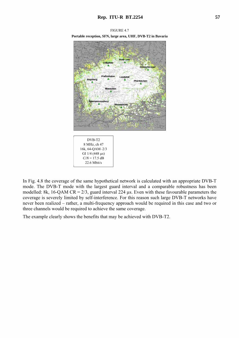
Rep. ITU-R BT.2254 57
FIGURE 4.7
Portable reception, SFN, large area, UHF, DVB-T2 in Bavaria
In Fig. 4.8 the coverage of the same hypothetical network is calculated with an appropriate DVB-T mode. The DVB-T mode with the largest guard interval and a comparable robustness has been modelled: 8k, 16-QAM CR = 2/3, guard interval 224 µs. Even with these favourable parameters the coverage is severely limited by self-interference. For this reason such large DVB-T networks have never been realized – rather, a multi-frequency approach would be required in this case and two or three channels would be required to achieve the same coverage.
The example clearly shows the benefits that may be achieved with DVB-T2.
DVB-T2 8 MHz, ch 47
16k, 64-QAM–2/3 GI 1/4 (448 µs) C/N = 17.5 dB
22.6 Mbit/s
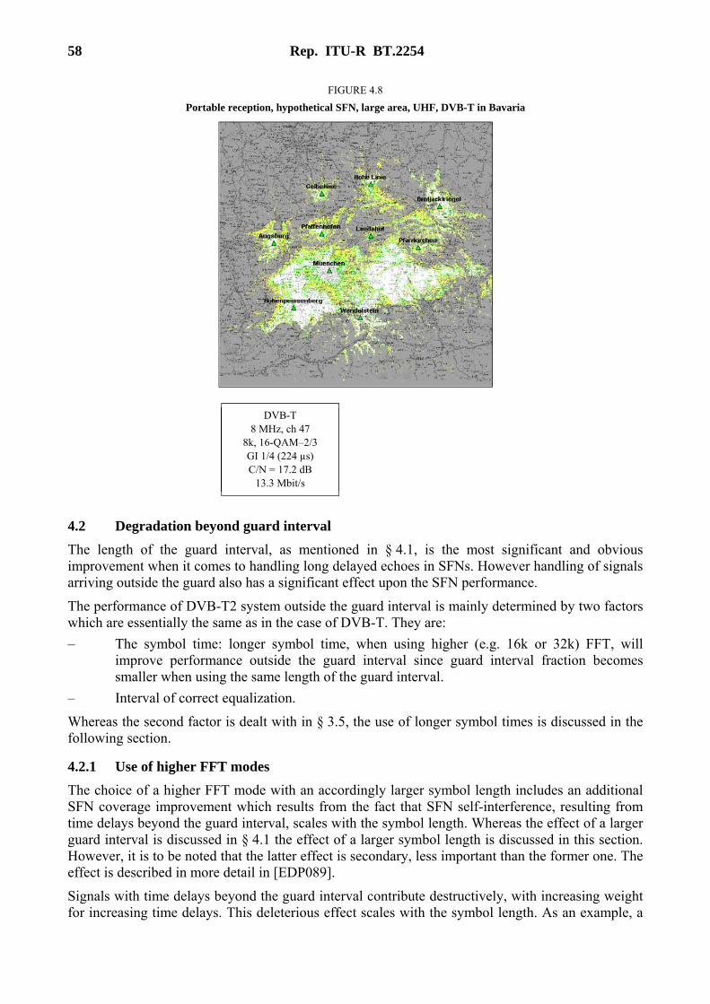
58 Rep. ITU-R BT.2254
FIGURE 4.8
Portable reception, hypothetical SFN, large area, UHF, DVB-T in Bavaria
4.2 Degradation beyond guard interval
The length of the guard interval, as mentioned in § 4.1, is the most significant and obvious improvement when it comes to handling long delayed echoes in SFNs. However handling of signals arriving outside the guard also has a significant effect upon the SFN performance.
The performance of DVB-T2 system outside the guard interval is mainly determined by two factors which are essentially the same as in the case of DVB-T. They are:
– The symbol time: longer symbol time, when using higher (e.g. 16k or 32k) FFT, will improve performance outside the guard interval since guard interval fraction becomes smaller when using the same length of the guard interval.
– Interval of correct equalization.
Whereas the second factor is dealt with in § 3.5, the use of longer symbol times is discussed in the following section.
4.2.1 Use of higher FFT modes
The choice of a higher FFT mode with an accordingly larger symbol length includes an additional SFN coverage improvement which results from the fact that SFN self-interference, resulting from time delays beyond the guard interval, scales with the symbol length. Whereas the effect of a larger guard interval is discussed in § 4.1 the effect of a larger symbol length is discussed in this section. However, it is to be noted that the latter effect is secondary, less important than the former one. The effect is described in more detail in [EDP089].
Signals with time delays beyond the guard interval contribute destructively, with increasing weight for increasing time delays. This deleterious effect scales with the symbol length. As an example, a
DVB-T 8 MHz, ch 47
8k, 16-QAM–2/3 GI 1/4 (224 µs) C/N = 17.2 dB
13.3 Mbit/s
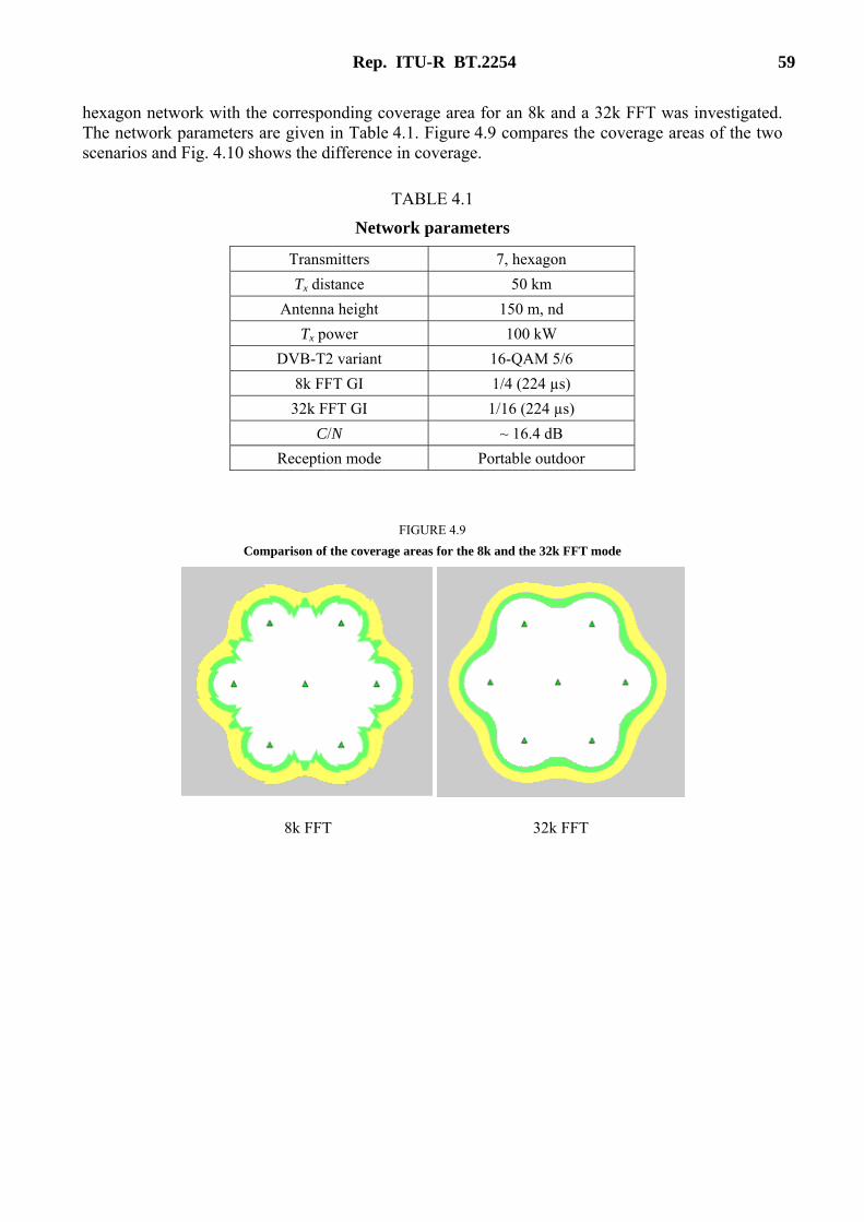
Rep. ITU-R BT.2254 59
hexagon network with the corresponding coverage area for an 8k and a 32k FFT was investigated. The network parameters are given in Table 4.1. Figure 4.9 compares the coverage areas of the two scenarios and Fig. 4.10 shows the difference in coverage.
TABLE 4.1
Network parameters
Transmitters 7, hexagon
Tx distance 50 km
Antenna height 150 m, nd
Tx power 100 kW
DVB-T2 variant 16-QAM 5/6
8k FFT GI 1/4 (224 µs)
32k FFT GI 1/16 (224 µs)
C/N ~ 16.4 dB
Reception mode Portable outdoor
FIGURE 4.9
Comparison of the coverage areas for the 8k and the 32k FFT mode
8k FFT 32k FFT
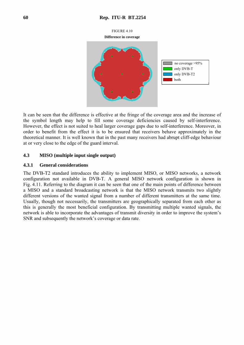
60 Rep. ITU-R BT.2254
FIGURE 4.10
Difference in coverage
It can be seen that the difference is effective at the fringe of the coverage area and the increase of the symbol length may help to fill some coverage deficiencies caused by self-interference. However, the effect is not suited to heal larger coverage gaps due to self-interference. Moreover, in order to benefit from the effect it is to be ensured that receivers behave approximately in the theoretical manner. It is well known that in the past many receivers had abrupt cliff-edge behaviour at or very close to the edge of the guard interval.
4.3 MISO (multiple input single output)
4.3.1 General considerations
The DVB-T2 standard introduces the ability to implement MISO, or MISO networks, a network configuration not available in DVB-T. A general MISO network configuration is shown in Fig. 4.11. Referring to the diagram it can be seen that one of the main points of difference between a MISO and a standard broadcasting network is that the MISO network transmits two slightly different versions of the wanted signal from a number of different transmitters at the same time. Usually, though not necessarily, the transmitters are geographically separated from each other as this is generally the most beneficial configuration. By transmitting multiple wanted signals, the network is able to incorporate the advantages of transmit diversity in order to improve the system’s SNR and subsequently the network’s coverage or data rate.
no coverage >95%
only DVB-T
only DVB-T2
both

Rep. ITU-R BT.2254 61
FIGURE 4.11
A general DVB-T2 MISO network
A DVB-T2 MISO network should be viewed as a particular form of an SFN, as the multiple transmissions require synchronization and timing in much the same way as a ‘standard’ SFN.
The DVB-T2 standard is based on a modified form of Alamouti’s scheme, one of a number of different possibilities. One of the main benefits of this particular scheme is that it can be implemented in a relatively straightforward manner that requires little additional complexity at both the transmit and receive sides of the network. Using only a single receive antenna the Alamouti scheme allows improvements in the received SNR equivalent to that obtained from a receive diversity system incorporating two receive antennas and a maximal ratio combining scheme. It also ensures that the ripples and notches that can form in a standard, two stations, SFN channel, which subsequently degrade the system’s SNR, do not occur in a MISO network as the two transmitted signals are no longer identical so destructive signal combination is essentially avoided. In a Gaussian channel, a 3 dB improvement in SNR could be achieved compared with the same network utilizing a ‘standard’ SFN. Slightly greater gains are possible in locations of similar receive levels. Although it is not without its trade-offs, Alamouti coding can improve coverage, allow a greater data rate or more efficient spectrum usage, or a combination of these outcomes.
The basic operation of the Alamouti based MISO network can be understood by referring to Fig. 4.11. Each of the network’s multiple transmitters is assigned to one of two Groups where each transmitter can be thought to transmit payload cells in pairs. Transmitters in Group 1 transmit an unmodified version of every constellation, just as they would in a ‘standard’ SFN – neither buffering nor negation or complex conjugation is applied. The first pair of cells is shown as C0 and C1 in the diagram. Transmitters in Group 2 however, transmit a slightly modified version of each constellation pair, and in reverse frequency order1. Group 2 transmits –C1* and C0* where * denotes the complex conjugation operation.
1 For example, if C0 is transmitted on carrier n for transmitters in Group 1, then C1 would be transmitted on carrier n + 1. Simultaneously, the transmitters in Group 2 would transmit –C1* on carrier n and C0* on carrier n + 1. The Alamouti coding is carried out in the frequency direction rather than the time direction.
62 Rep. ITU-R BT.2254
The receiver then recovers the components from the combined signals in a relatively straightforward manner that requires little additional complexity compared with a standard, non-MISO receiver.
The diagram also shows two pieces of equipment that are required in order for the network to operate correctly: the T2-Gateway and the DVB-T2 modulator. The T2-Gateway produces a T2-MI (T2-Modulator Interface) stream that contains all the information required to describe both the content and emission timing of T2-frames. The T2-MI stream is fed to the T2 modulators which apply the desired delays and the Alamouti coding.
As the diagram shows, all transmitters in the MISO network are locked to the same clock reference so the signals can be appropriately synchronized and delayed in a manner similar to a ‘standard’ SFN. Usually a GPS is used for this purpose.
It is also worth noting that the diagram shows an unlimited number of transmitters per Group. Although that is possible, it is not likely to occur in practice where two or three transmitters per Group would be more common.
4.3.2 Transmission parameter considerations
It should be noted that the DVB-T2 specification limits the maximum guard interval fraction (GIF) to 1/8. Subsequently, geographical SFN sizes could be limited. Furthermore, the scattered-pilot pattern chosen for a given FFT size and guard interval generally needs to be twice as dense because only half of the pilots are used for each of the sum and difference channel estimates – a factor that reduces capacity.
Both of the above factors should be considered when determining the suitability of a MISO network to a particular application.
4.3.3 Planning applications and considerations
In general, MISO should be considered for networks designed with a GIF up to 1/8 where capacity is not the limiting factor. In situations such as these where a ‘standard’ SFN might have been previously utilized, a MISO network may be more beneficial.
Moreover, the Alamouti coding is most beneficial when signals of equal magnitude from the two different transmitter groups are combined. Consideration should therefore be given to maximizing signal overlaps between the two groups as that would yield the largest gains. Conversely the scheme would be of limited benefit in networks with little overlap, particularly given the increased overhead.
Portable and mobile networks would typically be most likely to benefit from the scheme as they generally contain more omnidirectional reception antennas, which would increase the likelihood of similar strength signals overlapping. Furthermore, for these types of network and for mobile networks in particular, their transmitter network tend to be denser and the transmitters often have lower powers, which would likely increase overlaps further.
Perhaps the situation that a MISO network would most suit is one in which an area such as a large town is broadly served by two main transmitters which have overlapping signals. In this case one transmitter could be assigned to each transmitter group. The maximum potential of MISO might then be realized.
Fixed reception networks with relatively highly directional antennas may not be well suited to a MISO network unless the transmit antennas were located relatively close together so they fell roughly within the beam-width of a majority of the receive antennas. On the other hand, it may be possible to provide improvement to localised areas in such networks, particularly if the transmitters fell within the beam-width of the receive antennas.
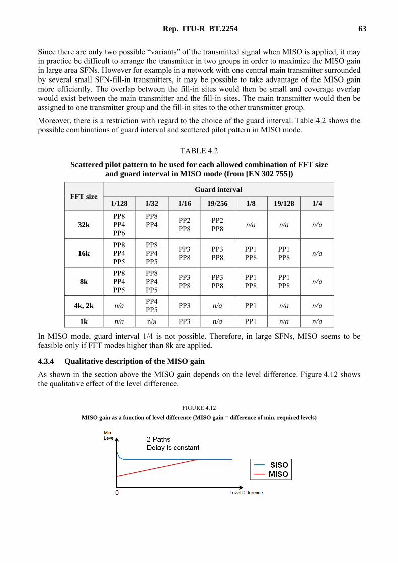
Rep. ITU-R BT.2254 63
Since there are only two possible “variants” of the transmitted signal when MISO is applied, it may in practice be difficult to arrange the transmitter in two groups in order to maximize the MISO gain in large area SFNs. However for example in a network with one central main transmitter surrounded by several small SFN-fill-in transmitters, it may be possible to take advantage of the MISO gain more efficiently. The overlap between the fill-in sites would then be small and coverage overlap would exist between the main transmitter and the fill-in sites. The main transmitter would then be assigned to one transmitter group and the fill-in sites to the other transmitter group.
Moreover, there is a restriction with regard to the choice of the guard interval. Table 4.2 shows the possible combinations of guard interval and scattered pilot pattern in MISO mode.
TABLE 4.2
Scattered pilot pattern to be used for each allowed combination of FFT size and guard interval in MISO mode (from [EN 302 755])
FFT size Guard interval
1/128 1/32 1/16 19/256 1/8 19/128 1/4
32k PP8 PP4 PP6
PP8 PP4
PP2 PP8
PP2 PP8
n/a n/a n/a
16k PP8 PP4 PP5
PP8 PP4 PP5
PP3 PP8
PP3 PP8
PP1 PP8
PP1 PP8
n/a
8k PP8 PP4 PP5
PP8 PP4 PP5
PP3 PP8
PP3 PP8
PP1 PP8
PP1 PP8
n/a
4k, 2k n/a PP4 PP5
PP3 n/a PP1 n/a n/a
1k n/a n/a PP3 n/a PP1 n/a n/a
In MISO mode, guard interval 1/4 is not possible. Therefore, in large SFNs, MISO seems to be feasible only if FFT modes higher than 8k are applied.
4.3.4 Qualitative description of the MISO gain
As shown in the section above the MISO gain depends on the level difference. Figure 4.12 shows the qualitative effect of the level difference.
FIGURE 4.12
MISO gain as a function of level difference (MISO gain = difference of min. required levels)

64 Rep. ITU-R BT.2254
Furthermore, the performance of MISO is also a function of the delay time. The channel estimation and/or correction is performed on pairs of cells, basically two adjacent sub-carriers. This means that MISO will work best if these adjacent sub-carriers are faded very similarly. This is the case for short delays. Long delays fade adjacent sub-carriers differently. Therefore an error is introduced that decreases the MISO effect. It might even occur at very large echoes that the MISO effect becomes a negative gain. The exact function needs to be verified by measurements. Figure 4.13 illustrates the qualitative effect of increasing delay.
FIGURE 4.13
MISO gain as a function of relative delay (MISO gain = difference of min. required levels)
Unfortunately, the implementation guideline [TS 102 831] does not yet give results of MISO simulations; but at least test scenarios are formulated, so that more reliable results can be expected soon.
4.3.5 Example of MISO coverage gain
In this example a coverage scenario with two transmitters is chosen [Ro2009]. The DVB-T2 parameters are 64-QAM, 8k, LDPC-code rate 3/4. Figure 4.14 shows the predicted coverage gain for distributed MISO, expressed in terms of gain of aggregated wanted field strength.
FIGURE 4.14
Predicted coverage gain with MISO
from [Ro2009]
Additional gain is achieved outside the core coverage areas of the two transmitters. With regard to acceptable indoor reception the coverage gain amounts to 30% in this simulation.
The above simulation is based on the assumption that MISO gain applies equally to all delay times between the signals from the two transmitters and that the only difference in MISO gain arises from
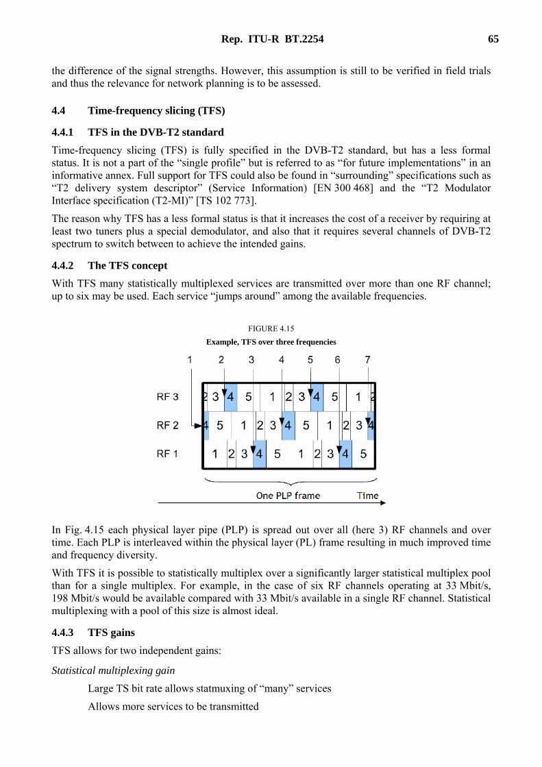
Rep. ITU-R BT.2254 65
the difference of the signal strengths. However, this assumption is still to be verified in field trials and thus the relevance for network planning is to be assessed.
4.4 Time-frequency slicing (TFS)
4.4.1 TFS in the DVB-T2 standard
Time-frequency slicing (TFS) is fully specified in the DVB-T2 standard, but has a less formal status. It is not a part of the “single profile” but is referred to as “for future implementations” in an informative annex. Full support for TFS could also be found in “surrounding” specifications such as “T2 delivery system descriptor” (Service Information) [EN 300 468] and the “T2 Modulator Interface specification (T2-MI)” [TS 102 773].
The reason why TFS has a less formal status is that it increases the cost of a receiver by requiring at least two tuners plus a special demodulator, and also that it requires several channels of DVB-T2 spectrum to switch between to achieve the intended gains.
4.4.2 The TFS concept
With TFS many statistically multiplexed services are transmitted over more than one RF channel; up to six may be used. Each service “jumps around” among the available frequencies.
FIGURE 4.15
Example, TFS over three frequencies
In Fig. 4.15 each physical layer pipe (PLP) is spread out over all (here 3) RF channels and over time. Each PLP is interleaved within the physical layer (PL) frame resulting in much improved time and frequency diversity.
With TFS it is possible to statistically multiplex over a significantly larger statistical multiplex pool than for a single multiplex. For example, in the case of six RF channels operating at 33 Mbit/s, 198 Mbit/s would be available compared with 33 Mbit/s available in a single RF channel. Statistical multiplexing with a pool of this size is almost ideal.
4.4.3 TFS gains
TFS allows for two independent gains:
Statistical multiplexing gain
Large TS bit rate allows statmuxing of “many” services
Allows more services to be transmitted
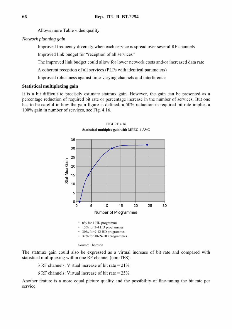
66 Rep. ITU-R BT.2254
Allows more Table video quality
Network planning gain
Improved frequency diversity when each service is spread over several RF channels
Improved link budget for “reception of all services”
The improved link budget could allow for lower network costs and/or increased data rate
A coherent reception of all services (PLPs with identical parameters)
Improved robustness against time-varying channels and interference
Statistical multiplexing gain
It is a bit difficult to precisely estimate statmux gain. However, the gain can be presented as a percentage reduction of required bit rate or percentage increase in the number of services. But one has to be careful in how the gain figure is defined; a 50% reduction in required bit rate implies a 100% gain in number of services, see Fig. 4.16.
FIGURE 4.16
Statistical multiplex gain with MPEG-4 AVC
• 0% for 1 HD programme • 15% for 3-4 HD programmes • 30% for 9-12 HD programmes • 32% for 18-24 HD programmes Source: Thomson
The statmux gain could also be expressed as a virtual increase of bit rate and compared with statistical multiplexing within one RF channel (non-TFS):
3 RF channels: Virtual increase of bit rate = 21%
6 RF channels: Virtual increase of bit rate = 25%
Another feature is a more equal picture quality and the possibility of fine-tuning the bit rate per service.
Rep. ITU-R BT.2254 67
Network planning gain
Without TFS the coverage of a set of multiplexes at a given location is limited by the multiplex with the lowest signal strength. With TFS the reception at a particular location is more likely to be determined by the average signal strength of the RF channels involved in TFS.
There are several components of the TFS network planning gain:
– TFS coverage gain
– TFS interference gain
– Improved robustness
4.4.4 TFS coverage gain
For a given equal ERP on multiple RF frequencies the received signal level, especially for fixed reception, varies significantly due to:
– Frequency-dependent transmitter antenna diagram
– Frequency-dependent terrain shielding (systematic)
– Frequency-dependent local variation (random)
– Frequency-dependent receiving antenna efficiency and gain (systematic and implementation dependent).
For each location, the TFS coverage gain could be expressed as the difference between the average signal strength and the minimum signal strength calculated over all RF frequencies at that particular location.
TFS coverage gain = P(average) – P(minimum) (dB)
4.4.5 TFS interference gain
TFS improves the robustness against static and time-varying interference from other transmitters, since interference level varies with frequency. For example, one frequency could be completely lost due to temporary interference.
4.4.6 Improved robustness
TFS improves the robustness against channel time variations (similar to RX diversity), especially important for portable/mobile reception.
4.4.7 Calculation of potential TFS coverage gain – example
The potential TFS coverage gain could be calculated based on field-strength measurements for a certain transmitter which transmits on more than one RF channel (multiplex).
In this example, the field measurements were performed for:
– Six transmitter sites (non SFN) with four multiplexes (frequencies) per site
– Equal ERP on all four frequencies
– About 40,000 measurements at a height of 3 m per measuring site
– Constant RX antenna gain.
The measured TFS gain distribution is based on the received signal strength on each frequency. In Fig. 4.17 the measured distribution of TFS gain for six stations A-F is shown.
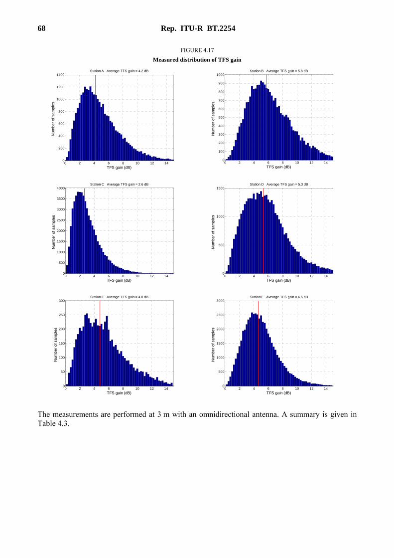
68 Rep. ITU-R BT.2254
FIGURE 4.17
Measured distribution of TFS gain
The measurements are performed at 3 m with an omnidirectional antenna. A summary is given in Table 4.3.
0 2 4 6 8 10 12 140
200
400
600
800
1000
1200
1400Station A Average TFS gain = 4.2 dB
TFS gain (dB)
Num
ber
of s
ampl
es
0 2 4 6 8 10 12 140
100
200
300
400
500
600
700
800
900
1000Station B Average TFS gain = 5.8 dB
TFS gain (dB)
Num
ber
of s
ampl
es
0 2 4 6 8 10 12 140
500
1000
1500
2000
2500
3000
3500
4000Station C Average TFS gain = 2.6 dB
TFS gain (dB)
Num
ber
of s
ampl
es
0 2 4 6 8 10 12 140
500
1000
1500Station D Average TFS gain = 5.3 dB
TFS gain (dB)
Num
ber
of s
ampl
es
0 2 4 6 8 10 12 140
50
100
150
200
250
300Station E Average TFS gain = 4.8 dB
TFS gain (dB)
Num
ber
of s
ampl
es
0 2 4 6 8 10 12 140
500
1000
1500
2000
2500
3000Station F Average TFS gain = 4.6 dB
TFS gain (dB)
Num
ber
of s
ampl
es

Rep. ITU-R BT.2254 69
TABLE 4.3
Summary of measurement results at 3 m
Station Average
TFS signal gain
Number of measurements
samples
Number of multiplexes
Channel number difference
A B
4.2 5.8
27 000 30 000
4 4
16 34
C 2.6 58 000 4 15
D E
5.3 4.8
41 000 6 000
4 4
32 24
F 4.6 56 000 4 26
The average TFS gain over all six areas is 4.5 dB.
4.4.8 Coherent coverage effects
In case each PLP has the same parameters, the coverage of all PLPs will be very similar, if not, identical.
A further aspect is the “common coverage shrinking”. TFS uses several RF channels at a time. If one RF channel fails (transmitter failure) the coverage will then shrink but not completely vanish. Only the outer part of the coverage is affected in that case. The more RF channels that are combined, the less is the loss of coverage when one channel fails.
4.5 Time slicing
The DVB-T2 specification allows for time slicing, which is a well-known DVB-H feature. Time slicing reduces the energy consumption of the receiving device. This is achieved by transmitting the services of a multiplex in time blocks which allows the receiver to demodulate the signal only for a certain fraction of time in order to receive a particular service. For the rest of the time the receiver may remain idle, it may use the remaining time for the check of other frequency blocks or channels.
4.6 Physical layer pipes
4.6.1 Input streams and physical layer pipes
The commercial requirement for service-specific robustness together with the need for different stream types is met by the concept of fully transparent PLPs. Both the allocated capacity and the robustness can be adjusted to the content/service providers’ particular needs, depending on the type of receiver and the receiving conditions to be addressed.
The DVB-T2 specification allows a constellation, code rate and time-interleaving depth to be assigned individually to each single PLP. A high level T2 block diagram is shown in Fig. 4.18.
Input streams are MPEG-2 transport streams (TS) or so called generic streams which could carry MPEG-2 or MPEG-4 video content. Each input stream is carried by a corresponding PLP in DVB-T2. A maximum of 255 input streams/PLPs could be transmitted with, typically, one service per TS/PLP.
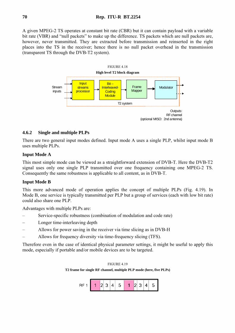
70 Rep. ITU-R BT.2254
A given MPEG-2 TS operates at constant bit rate (CBR) but it can contain payload with a variable bit rate (VBR) and “null packets” to make up the difference. TS packets which are null packets are, however, never transmitted. They are extracted before transmission and reinserted in the right places into the TS in the receiver; hence there is no null packet overhead in the transmission (transparent TS through the DVB-T2 system).
FIGURE 4.18
High level T2 block diagram
Bit –
Interleaved- Coding Module
Frame Mapper
Modulator Stream
inputs
Outputs: RF channel
(optional MISO: 2nd antenna)
Input streams
processor
T2 system
4.6.2 Single and multiple PLPs
There are two general input modes defined. Input mode A uses a single PLP, whilst input mode B uses multiple PLPs.
Input Mode A
This most simple mode can be viewed as a straightforward extension of DVB-T. Here the DVB-T2 signal uses only one single PLP transmitted over one frequency containing one MPEG-2 TS. Consequently the same robustness is applicable to all content, as in DVB-T.
Input Mode B
This more advanced mode of operation applies the concept of multiple PLPs (Fig. 4.19). In Mode B, one service is typically transmitted per PLP but a group of services (each with low bit rate) could also share one PLP.
Advantages with multiple PLPs are:
– Service-specific robustness (combination of modulation and code rate)
– Longer time-interleaving depth
– Allows for power saving in the receiver via time slicing as in DVB-H
– Allows for frequency diversity via time-frequency slicing (TFS).
Therefore even in the case of identical physical parameter settings, it might be useful to apply this mode, especially if portable and/or mobile devices are to be targeted.
FIGURE 4.19
T2 frame for single RF channel, multiple PLP mode (here, five PLPs)

Rep. ITU-R BT.2254 71
Typically a group of services will share common elements such as PSI/SI tables, like EPG information, or CA information. To avoid the need to duplicate this information for each PLP, Mode B offers the concept of common PLPs, shared by a group of PLPs. Hence, receivers need to decode up to two PLPs at the same time when receiving a single service: the data PLP and the common PLP.
FIGURE 4.20
Example of a DVB-T2 multiplex using PLP and carrying services with different data rates and different coverage radii
An example is given in Fig. 4.20 where four different classes of services (HDTV, SDTV, Audio Broadcasting and Data Broadcasting) are carried in one multiplex. Each of the services has a different data rate and a different coverage radius indicated in the Figure on the right hand side.
Additional advantages with multiple PLPs are:
– Different types of receivers and different reception cases could be addressed by the same signal, for example HDTV to fixed rooftop aerials and mobile receivers simultaneously, with a certain capacity and robustness for each category.
– One could prioritize the robustness for one or many services in one multiplex prioritized services “last longer”.
– When one service in a multiplex does not need to have the same coverage as the other, that service could be transmitted with lower robustness saving transmission capacity.
– Simplifies the change to local/regional content (with constant bit rate) in a multiplex in which the rest of the content is centrally statistically multiplexed. The use of one dedicated PLP for local/regional content could result in an easier/cheaper implementation.
– When one wish to further increase the capacity and coverage by using the TFS concept.
One limitation with the use of PLPs is that it is not possible to have PLPs with different FFT sizes in the same multiplex. This could for example be a limitation when there is the need to provide rooftop reception for HD services and a mobile service in the same multiplex, using a large area SFN.
In order not to lose capacity there may then be a need to use the 32k FFT mode for the HD services. With the long symbol time it is possible to use a lower guard interval fraction, thus maximizing capacity. However if the 32k mode is used it will mean that the frequency distance between the OFDM carriers is short, which will make the mobile service sensitive to Doppler shift at higher speeds.
This limitation might be overcome by using the future extension frame (FEF), see § 4.8.
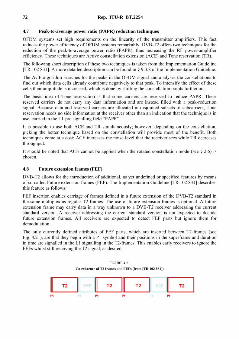
72 Rep. ITU-R BT.2254
4.7 Peak-to-average power ratio (PAPR) reduction techniques
OFDM systems set high requirements on the linearity of the transmitter amplifiers. This fact reduces the power efficiency of OFDM systems remarkably. DVB-T2 offers two techniques for the reduction of the peak-to-average power ratio (PAPR), thus increasing the RF power-amplifier efficiency. These techniques are Active constellation extension (ACE) and Tone reservation (TR).
The following short description of these two techniques is taken from the Implementation Guideline [TR 102 831]. A more detailed description can be found in § 9.3.8 of the Implementation Guideline.
The ACE algorithm searches for the peaks in the OFDM signal and analyses the constellations to find out which data cells already contribute negatively to that peak. To intensify the effect of these cells their amplitude is increased, which is done by shifting the constellation points further out.
The basic idea of Tone reservation is that some carriers are reserved to reduce PAPR. These reserved carriers do not carry any data information and are instead filled with a peak-reduction signal. Because data and reserved carriers are allocated in disjointed subsets of subcarriers, Tone reservation needs no side information at the receiver other than an indication that the technique is in use, carried in the L1-pre signalling field “PAPR”.
It is possible to use both ACE and TR simultaneously; however, depending on the constellation, picking the better technique based on the constellation will provide most of the benefit. Both techniques come at a cost: ACE increases the noise level that the receiver sees while TR decreases throughput.
It should be noted that ACE cannot be applied when the rotated constellation mode (see § 2.6) is chosen.
4.8 Future extension frames (FEF)
DVB-T2 allows for the introduction of additional, as yet undefined or specified features by means of so-called Future extension frames (FEF). The Implementation Guideline [TR 102 831] describes this feature as follows:
FEF insertion enables carriage of frames defined in a future extension of the DVB-T2 standard in the same multiplex as regular T2-frames. The use of future extension frames is optional. A future extension frame may carry data in a way unknown to a DVB-T2 receiver addressing the current standard version. A receiver addressing the current standard version is not expected to decode future extension frames. All receivers are expected to detect FEF parts but ignore them for demodulation.
The only currently defined attributes of FEF parts, which are inserted between T2-frames (see Fig. 4.21), are that they begin with a P1 symbol and their positions in the superframe and duration in time are signalled in the L1 signalling in the T2-frames. This enables early receivers to ignore the FEFs whilst still receiving the T2 signal, as desired.
FIGURE 4.21
Co-existence of T2 frames and FEFs (from [TR 102 831])

Rep. ITU-R BT.2254 73
FEFs can be used for Transmitter Signatures [A150]. They allow measurements to identify which echo (path) in the channel impulse response originates from which transmitter of the SFN. It is also possible to display the parts of the channel impulse response originating from individual transmitters of the SFN.
FEFs could also be used, for example, for:
– Handheld services with MIMO support
– Upstream for a DVB-T2 return channel
– Data transport of mobile service providers which use the same spectrum but have a different network structure.
An already existing application is the particular DVB-T2 profile T2-Lite which is described in Annex 5.
More details on FEF can be found in [TR 102 831, § 8.4].
5 Implementation scenarios
5.1 Introduction
DVB-T2 offers a significantly wider choice of parameters (which is described in § 2) than did DVB-T. The choice is so large that it is not possible to consider all of their possible combinations. This section considers a number of common applications of DVB-T2 and discusses some possible parameter sets which may be suitable for each of the scenarios.
Firstly, a number of scenarios appropriate to fixed roof-level reception are described. They comprise an MFN as well as an SFN approach and also reflect the need for a transition from DVB-T to DVB-T2, which is likely to be a common requirement.
Secondly, five scenarios particularly suited to portable and mobile DTT reception are described. All five scenarios are based on an SFN approach and include relatively large guard intervals to minimize intra-SFN interference and to allow greater transmitter separation. The 32k FFT mode is not applied for the same reason, since it is expected that this mode is particularly vulnerable to Doppler degradation and may be unsuitable for mobile and portable networks.
Parameters are based on the information given in the ETSI specification and Implementation Guideline [TS 102 831, EN 302 755]. C/N figures are derived according to the methodology described in § 2.5 and respective data rates according to Annex 2. In scenarios 1 and 4 the parameters of a corresponding DVB-T mode are also given for comparison. The C/N values for DVB-T are taken from the respective ETSI specification [EN 300 744], including an implementation margin of 3 dB.
5.2 Scenario 1: MFN rooftop reception and a transition case
A number of countries will wish to move from an established DVB-T network to one using DVB-T2. This scenario provides an example of how that transition might take place while incorporating some common practical considerations.
Although DVB-T2 may make it possible to improve or optimize the coverage of an existing network, in many cases the existing network’s coverage would be considered sufficient and it would therefore be desirable to keep the coverage constant while increasing its capacity as that would allow new services to be introduced. In such situations, it would be desirable to reuse the existing infrastructure such as the transmission stations, transmitters, combiners and antenna systems. The example below would allow this type of transition with a minimum of changes –

74 Rep. ITU-R BT.2254
essentially the only requirement being the upgrade of modulators. The transmission side of the network, otherwise unchanged, would maintain essentially constant coverage.2
For comparison, two sets of parameters are provided, one for the DVB-T network and another for the DVB-T2. Importantly, both sets of parameters result in a similar C/N, meaning that if the transmit antennas and powers of the DVB-T network are maintained for DVB-T2, the network’s coverage would essentially remain unchanged. Both sets of parameters also exhibit the same guard interval duration despite the guard interval fraction being substantially reduced for the DVB-T2 case. Again, if the transmit antennas and radiated powers remained constant in both networks, the SFN timings of the DVB-T network would translate directly to the DVB-T2 network with little change in coverage.
DVB-T parameters DVB-T2 parameters
Bandwidth: 8 MHz Bandwidth: 8 MHz
FFT size: 2k FFT size: 32k
Carrier mode: N/A Carrier mode: extended
Scattered pilot pattern: N/A Scattered pilot pattern: PP7
Guard interval: 1/32 (7 µs) Guard interval: 1/128 (28 µs)
Modulation: 64-QAM Modulation: 256-QAM
Code rate: 2/3 Code rate: 2/3
C/N (Rice): 20.1 dB C/N (Rice): 20.0 dB
Resulting data rate: 24.1 Mbit/s Resulting data rate: 40.2 Mbit/s
5.3 Scenario 2: SFN rooftop reception, maximum coverage
This scenario is intended to maximize coverage in an SFN while providing rooftop reception. In this case it is necessary to use a relatively robust DVB-T2 mode. Several possible lengths of the guard interval may be possible depending on the network structure to be used, transmitter distance, radiated powers and terrain. Because of the relatively high robustness of the mode, it may be possible to reduce the guard interval to 1/16 (224 µs) for very large SFNs – a change that would increase capacity.
Bandwidth: 8 MHz
FFT size: 32k
Carrier mode: extended
Scattered pilot pattern: PP2
Guard interval: 1/8 (448 µs)
Modulation: 16-QAM
Code rate: 2/3
C/N (Rice): 11.6 dB
Resulting data rate: 16.7 Mbit/s
2 Changes to the distribution network and other similar details have not been considered.
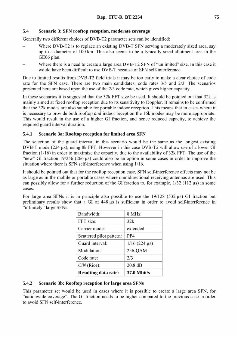
Rep. ITU-R BT.2254 75
5.4 Scenario 3: SFN rooftop reception, moderate coverage
Generally two different choices of DVB-T2 parameter sets can be identified:
– Where DVB-T2 is to replace an existing DVB-T SFN serving a moderately sized area, say up to a diameter of 100 km. This also seems to be a typically sized allotment area in the GE06 plan.
– Where there is a need to create a large area DVB-T2 SFN of “unlimited” size. In this case it would have been difficult to use DVB-T because of SFN self-interference.
Due to limited results from DVB-T2 field trials it may be too early to make a clear choice of code rate for the SFN case. There are two main candidates; code rates 3/5 and 2/3. The scenarios presented here are based upon the use of the 2/3 code rate, which gives higher capacity.
In these scenarios it is suggested that the 32k FFT size be used. It should be pointed out that 32k is mainly aimed at fixed rooftop reception due to its sensitivity to Doppler. It remains to be confirmed that the 32k modes are also suitable for portable indoor reception. This means that in cases where it is necessary to provide both rooftop and indoor reception the 16k modes may be more appropriate. This would result in the use of a higher GI fraction, and hence reduced capacity, to achieve the required guard interval duration.
5.4.1 Scenario 3a: Rooftop reception for limited area SFN
The selection of the guard interval in this scenario would be the same as the longest existing DVB-T mode (224 µs), using 8k FFT. However in this case DVB-T2 will allow use of a lower GI fraction (1/16) in order to maximize the capacity, due to the availability of 32k FFT. The use of the “new” GI fraction 19/256 (266 µs) could also be an option in some cases in order to improve the situation where there is SFN self-interference when using 1/16.
It should be pointed out that for the rooftop reception case, SFN self-interference effects may not be as large as in the mobile or portable cases where omnidirectional receiving antennas are used. This can possibly allow for a further reduction of the GI fraction to, for example, 1/32 (112 µs) in some cases.
For large area SFNs it is in principle also possible to use the 19/128 (532 µs) GI fraction but preliminary results show that a GI of 448 µs is sufficient in order to avoid self-interference in “infinitely” large SFNs.
Bandwidth: 8 MHz
FFT size: 32k
Carrier mode: extended
Scattered pilot pattern: PP4
Guard interval: 1/16 (224 µs)
Modulation: 256-QAM
Code rate: 2/3
C/N (Rice): 20.8 dB
Resulting data rate: 37.0 Mbit/s
5.4.2 Scenario 3b: Rooftop reception for large area SFNs
This parameter set would be used in cases where it is possible to create a large area SFN, for “nationwide coverage”. The GI fraction needs to be higher compared to the previous case in order to avoid SFN self-interference.
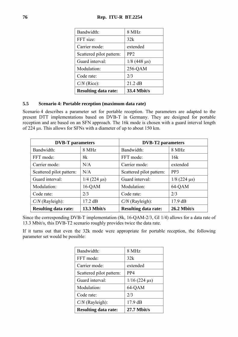
76 Rep. ITU-R BT.2254
Bandwidth: 8 MHz
FFT size: 32k
Carrier mode: extended
Scattered pilot pattern: PP2
Guard interval: 1/8 (448 µs)
Modulation: 256-QAM
Code rate: 2/3
C/N (Rice): 21.2 dB
Resulting data rate: 33.4 Mbit/s
5.5 Scenario 4: Portable reception (maximum data rate)
Scenario 4 describes a parameter set for portable reception. The parameters are adapted to the present DTT implementations based on DVB-T in Germany. They are designed for portable reception and are based on an SFN approach. The 16k mode is chosen with a guard interval length of 224 µs. This allows for SFNs with a diameter of up to about 150 km.
DVB-T parameters DVB-T2 parameters
Bandwidth: 8 MHz Bandwidth: 8 MHz
FFT mode: 8k FFT mode: 16k
Carrier mode: N/A Carrier mode: extended
Scattered pilot pattern: N/A Scattered pilot pattern: PP3
Guard interval: 1/4 (224 µs) Guard interval: 1/8 (224 µs)
Modulation: 16-QAM Modulation: 64-QAM
Code rate: 2/3 Code rate: 2/3
C/N (Rayleigh): 17.2 dB C/N (Rayleigh): 17.9 dB
Resulting data rate: 13.3 Mbit/s Resulting data rate: 26.2 Mbit/s
Since the corresponding DVB-T implementation (8k, 16-QAM-2/3, GI 1/4) allows for a data rate of 13.3 Mbit/s, this DVB-T2 scenario roughly provides twice the data rate.
If it turns out that even the 32k mode were appropriate for portable reception, the following parameter set would be possible:
Bandwidth: 8 MHz
FFT mode: 32k
Carrier mode: extended
Scattered pilot pattern: PP4
Guard interval: 1/16 (224 µs)
Modulation: 64-QAM
Code rate: 2/3
C/N (Rayleigh): 17.9 dB
Resulting data rate: 27.7 Mbit/s
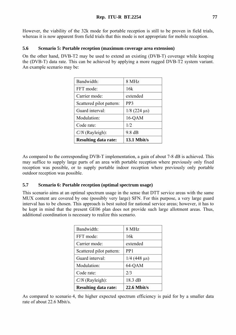
Rep. ITU-R BT.2254 77
However, the viability of the 32k mode for portable reception is still to be proven in field trials, whereas it is now apparent from field trials that this mode is not appropriate for mobile reception.
5.6 Scenario 5: Portable reception (maximum coverage area extension)
On the other hand, DVB-T2 may be used to extend an existing (DVB-T) coverage while keeping the (DVB-T) data rate. This can be achieved by applying a more rugged DVB-T2 system variant. An example scenario may be:
Bandwidth: 8 MHz
FFT mode: 16k
Carrier mode: extended
Scattered pilot pattern: PP3
Guard interval: 1/8 (224 µs)
Modulation: 16-QAM
Code rate: 1/2
C/N (Rayleigh): 9.8 dB
Resulting data rate: 13.1 Mbit/s
As compared to the corresponding DVB-T implementation, a gain of about 7-8 dB is achieved. This may suffice to supply large parts of an area with portable reception where previously only fixed reception was possible, or to supply portable indoor reception where previously only portable outdoor reception was possible.
5.7 Scenario 6: Portable reception (optimal spectrum usage)
This scenario aims at an optimal spectrum usage in the sense that DTT service areas with the same MUX content are covered by one (possibly very large) SFN. For this purpose, a very large guard interval has to be chosen. This approach is best suited for national service areas; however, it has to be kept in mind that the present GE06 plan does not provide such large allotment areas. Thus, additional coordination is necessary to realize this scenario.
Bandwidth: 8 MHz
FFT mode: 16k
Carrier mode: extended
Scattered pilot pattern: PP1
Guard interval: 1/4 (448 µs)
Modulation: 64-QAM
Code rate: 2/3
C/N (Rayleigh): 18.3 dB
Resulting data rate: 22.6 Mbit/s
As compared to scenario 4, the higher expected spectrum efficiency is paid for by a smaller data rate of about 22.6 Mbit/s.
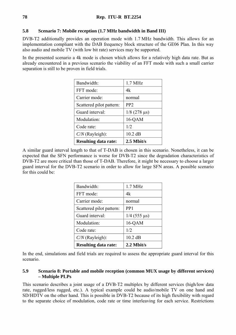
78 Rep. ITU-R BT.2254
5.8 Scenario 7: Mobile reception (1.7 MHz bandwidth in Band III)
DVB-T2 additionally provides an operation mode with 1.7 MHz bandwidth. This allows for an implementation compliant with the DAB frequency block structure of the GE06 Plan. In this way also audio and mobile TV (with low bit rate) services may be supported.
In the presented scenario a 4k mode is chosen which allows for a relatively high data rate. But as already encountered in a previous scenario the viability of an FFT mode with such a small carrier separation is still to be proven in field trials.
Bandwidth: 1.7 MHz
FFT mode: 4k
Carrier mode: normal
Scattered pilot pattern: PP2
Guard interval: 1/8 (278 µs)
Modulation: 16-QAM
Code rate: 1/2
C/N (Rayleigh): 10.2 dB
Resulting data rate: 2.5 Mbit/s
A similar guard interval length to that of T-DAB is chosen in this scenario. Nonetheless, it can be expected that the SFN performance is worse for DVB-T2 since the degradation characteristics of DVB-T2 are more critical than those of T-DAB. Therefore, it might be necessary to choose a larger guard interval for the DVB-T2 scenario in order to allow for large SFN areas. A possible scenario for this could be:
Bandwidth: 1.7 MHz
FFT mode: 4k
Carrier mode: normal
Scattered pilot pattern: PP1
Guard interval: 1/4 (555 µs)
Modulation: 16-QAM
Code rate: 1/2
C/N (Rayleigh): 10.2 dB
Resulting data rate: 2.2 Mbit/s
In the end, simulations and field trials are required to assess the appropriate guard interval for this scenario.
5.9 Scenario 8: Portable and mobile reception (common MUX usage by different services) – Multiple PLPs
This scenario describes a joint usage of a DVB-T2 multiplex by different services (high/low data rate, rugged/less rugged, etc.). A typical example could be audio/mobile TV on one hand and SD/HDTV on the other hand. This is possible in DVB-T2 because of its high flexibility with regard to the separate choice of modulation, code rate or time interleaving for each service. Restrictions
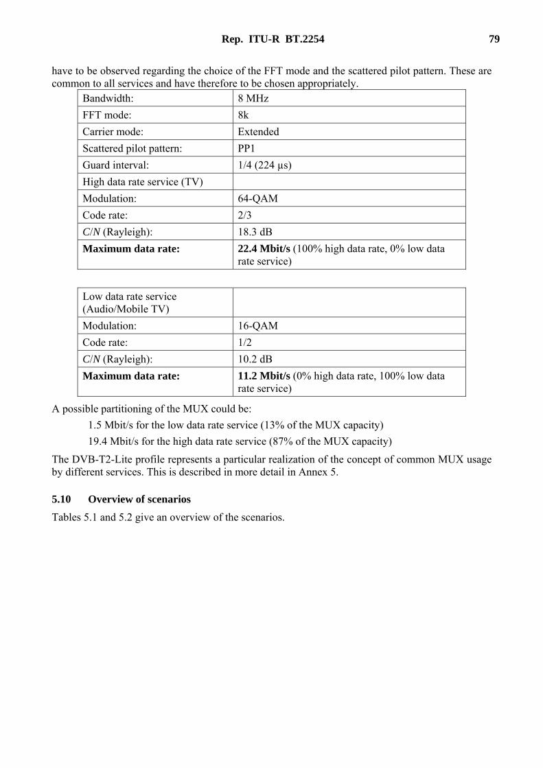
Rep. ITU-R BT.2254 79
have to be observed regarding the choice of the FFT mode and the scattered pilot pattern. These are common to all services and have therefore to be chosen appropriately.
Bandwidth: 8 MHz
FFT mode: 8k
Carrier mode: Extended
Scattered pilot pattern: PP1
Guard interval: 1/4 (224 µs)
High data rate service (TV)
Modulation: 64-QAM
Code rate: 2/3
C/N (Rayleigh): 18.3 dB
Maximum data rate: 22.4 Mbit/s (100% high data rate, 0% low data rate service)
Low data rate service (Audio/Mobile TV)
Modulation: 16-QAM
Code rate: 1/2
C/N (Rayleigh): 10.2 dB
Maximum data rate: 11.2 Mbit/s (0% high data rate, 100% low data rate service)
A possible partitioning of the MUX could be:
1.5 Mbit/s for the low data rate service (13% of the MUX capacity)
19.4 Mbit/s for the high data rate service (87% of the MUX capacity)
The DVB-T2-Lite profile represents a particular realization of the concept of common MUX usage by different services. This is described in more detail in Annex 5.
5.10 Overview of scenarios
Tables 5.1 and 5.2 give an overview of the scenarios.
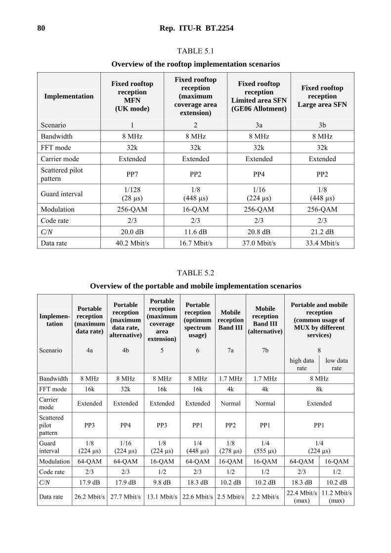
80 Rep. ITU-R BT.2254
TABLE 5.1
Overview of the rooftop implementation scenarios
Implementation
Fixed rooftop reception
MFN (UK mode)
Fixed rooftop reception
(maximum coverage area
extension)
Fixed rooftop reception
Limited area SFN (GE06 Allotment)
Fixed rooftop reception
Large area SFN
Scenario 1 2 3a 3b
Bandwidth 8 MHz 8 MHz 8 MHz 8 MHz
FFT mode 32k 32k 32k 32k
Carrier mode Extended Extended Extended Extended
Scattered pilot pattern
PP7 PP2 PP4 PP2
Guard interval 1/128
(28 µs) 1/8
(448 µs) 1/16
(224 µs) 1/8
(448 µs)
Modulation 256-QAM 16-QAM 256-QAM 256-QAM
Code rate 2/3 2/3 2/3 2/3
C/N 20.0 dB 11.6 dB 20.8 dB 21.2 dB
Data rate 40.2 Mbit/s 16.7 Mbit/s 37.0 Mbit/s 33.4 Mbit/s
TABLE 5.2
Overview of the portable and mobile implementation scenarios
Implemen-tation
Portable reception
(maximum data rate)
Portable reception
(maximum data rate,
alternative)
Portable reception
(maximum coverage
area extension)
Portable reception(optimum spectrum
usage)
Mobile receptionBand III
Mobile reception Band III
(alternative)
Portable and mobile reception
(common usage of MUX by different
services)
Scenario 4a 4b 5 6 7a 7b 8
high data
rate low data
rate
Bandwidth 8 MHz 8 MHz 8 MHz 8 MHz 1.7 MHz 1.7 MHz 8 MHz
FFT mode 16k 32k 16k 16k 4k 4k 8k
Carrier mode
Extended Extended Extended Extended Normal Normal Extended
Scattered pilot pattern
PP3 PP4 PP3 PP1 PP2 PP1 PP1
Guard interval
1/8 (224 µs)
1/16 (224 µs)
1/8 (224 µs)
1/4 (448 µs)
1/8 (278 µs)
1/4 (555 µs)
1/4 (224 µs)
Modulation 64-QAM 64-QAM 16-QAM 64-QAM 16-QAM 16-QAM 64-QAM 16-QAM
Code rate 2/3 2/3 1/2 2/3 1/2 1/2 2/3 1/2
C/N 17.9 dB 17.9 dB 9.8 dB 18.3 dB 10.2 dB 10.2 dB 18.3 dB 10.2 dB
Data rate 26.2 Mbit/s 27.7 Mbit/s 13.1 Mbit/s 22.6 Mbit/s 2.5 Mbit/s 2.2 Mbit/s 22.4 Mbit/s
(max) 11.2 Mbit/s
(max)

Rep. ITU-R BT.2254 81
6 Transition to DVB-T2
6.1 DVB-T2 in GE06
6.1.1 Implementing alternative broadcasting transmission systems under the GE06 Agreement
The RRC-06 adopted DVB-T and T-DAB as the two transmission systems for which the GE06 Plan was developed. Contracting Members of the GE06 Agreement adopted these two transmission systems as the only transmission systems for modifying the Plan and their Plan entries. Furthermore, the Plan modification procedures of Article 4 have been developed specifically in terms of these two transmission systems. The result is that only these two transmission systems can be used when submitting modifications to the Plan. This implies that if a Contracting Member of the GE06 Agreement wants to implement assignments using DVB-T2 or another transmission system, then such assignments must first be submitted as Plan modifications using suitable technical characteristics and either indicating T-DAB or DVB-T as the transmission system.
When the Plan entry is brought into operation the administration can notify the actual transmission system (e.g. DVB-T2, DVB-H or any other suitable system) under the Article 5 provision 5.1.3 of the agreement. Under this provision such an implementation is restricted not to cause more interference or require a higher level of protection than the original Plan entry. Additionally, the peak power density over any 4 kHz of such an implementation should not exceed the peak power density in the same 4 kHz of the corresponding digital broadcasting Plan entry.
The ITU-R has prepared the notice form GB1 for the notification of a DVB-T2 assignment.
6.1.2 Requirements for the development of the DVB-T2 specification
It was felt essential that DVB-T2 implementations should be able to use DVB-T assignments and allotments of the GE06 Plan in order to avoid re-planning activities and therefore adding complexity to the introduction of DVB-T2. The commercial requirements for the development of the DVB-T2 specification therefore include the following: “Transmissions using the DVB-T2 specification shall meet the interference levels and spectrum mask requirements as defined by GE06 and not cause more interference than DVB-T would do.”
With respect to DVB-T as planned in the GE06 Plan, DVB-T2:
– offers the same or better protection ratios and comparable minimum median field strength values for suitable equivalent variants;
– can use the same linear (single or mixed) polarization of the digital broadcasting Plan entry;
– can realize the same service areas using the same or lower radiated power levels;
– maintains the same or lower peak power densities for variants operating in the same bandwidth and having the same or higher number of OFDM carriers (FFT size) for the same levels of radiated power.
6.1.3 Implementation of DVB-T2 in the GE06 Plan
DVB-T2 offers sufficient flexibility in terms of the number of suitable equivalent variants that would maintain the same service area and would permit the operation of an assignment(s) within the limitations of Provision 5.1.3 of the GE06 Agreement and a corresponding digital broadcasting Plan entry. Additionally, in order to ensure that a DVB-T2 implementation respects the radiated power limitations outside the operating bandwidth, the DVB-T2 implementation will have to conform with the spectrum mask of the corresponding GE06 Plan entry as given in the GE06 Agreement in Fig. 3-2 and Table 3-10 (of the Agreement text) for T-DAB Plan entries and Fig. 3-3 and Table 3-11 for DVB-T Plan entries. Furthermore, the technical characteristics of the DVB-T2 implementation
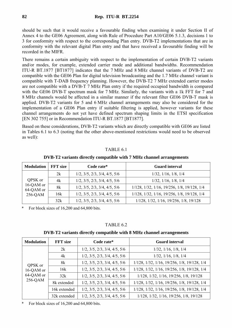
82 Rep. ITU-R BT.2254
should be such that it would receive a favourable finding when examining it under Section II of Annex 4 to the GE06 Agreement, along with Rule of Procedure Part A10/GE06 5.1.3, decisions 1 to 3 for conformity with respect to the corresponding Plan entry. DVB-T2 implementations that are in conformity with the relevant digital Plan entry and that have received a favourable finding will be recorded in the MIFR.
There remains a certain ambiguity with respect to the implementation of certain DVB-T2 variants and/or modes, for example, extended carrier mode and additional bandwidths. Recommendation ITU-R BT.1877 [BT1877] indicates that the 7 MHz and 8 MHz channel variants of DVB-T2 are compatible with the GE06 Plan for digital television broadcasting and the 1.7 MHz channel variant is compatible with T-DAB frequency planning. However, the DVB-T2 7 MHz extended carrier modes are not compatible with a DVB-T 7 MHz Plan entry if the required occupied bandwidth is compared with the GE06 DVB-T spectrum mask for 7 MHz. Similarly, the variants with a 1k FFT for 7 and 8 MHz channels would be affected in a similar manner if the relevant filter GE06 DVB-T mask is applied. DVB-T2 variants for 5 and 6 MHz channel arrangements may also be considered for the implementation of a GE06 Plan entry if suitable filtering is applied, however variants for these channel arrangements do not yet have defined spectrum shaping limits in the ETSI specification [EN 302 755] or in Recommendation ITU-R BT.1877 [BT1877].
Based on these considerations, DVB-T2 variants which are directly compatible with GE06 are listed in Tables 6.1 to 6.3 (noting that the other above-mentioned restrictions would need to be observed as well):
TABLE 6.1
DVB-T2 variants directly compatible with 7 MHz channel arrangements
Modulation FFT size Code rate* Guard interval
QPSK or 16-QAM or 64-QAM or 256-QAM
2k 1/2, 3/5, 2/3, 3/4, 4/5, 5/6 1/32, 1/16, 1/8, 1/4
4k 1/2, 3/5, 2/3, 3/4, 4/5, 5/6 1/32, 1/16, 1/8, 1/4
8k 1/2, 3/5, 2/3, 3/4, 4/5, 5/6 1/128, 1/32, 1/16, 19/256, 1/8, 19/128, 1/4
16k 1/2, 3/5, 2/3, 3/4, 4/5, 5/6 1/128, 1/32, 1/16, 19/256, 1/8, 19/128, 1/4
32k 1/2, 3/5, 2/3, 3/4, 4/5, 5/6 1/128, 1/32, 1/16, 19/256, 1/8, 19/128
* For block sizes of 16,200 and 64,800 bits.
TABLE 6.2
DVB-T2 variants directly compatible with 8 MHz channel arrangements
Modulation FFT size Code rate* Guard interval
QPSK or 16-QAM or 64-QAM or 256-QAM
2k 1/2, 3/5, 2/3, 3/4, 4/5, 5/6 1/32, 1/16, 1/8, 1/4
4k 1/2, 3/5, 2/3, 3/4, 4/5, 5/6 1/32, 1/16, 1/8, 1/4
8k 1/2, 3/5, 2/3, 3/4, 4/5, 5/6 1/128, 1/32, 1/16, 19/256, 1/8, 19/128, 1/4
16k 1/2, 3/5, 2/3, 3/4, 4/5, 5/6 1/128, 1/32, 1/16, 19/256, 1/8, 19/128, 1/4
32k 1/2, 3/5, 2/3, 3/4, 4/5, 5/6 1/128, 1/32, 1/16, 19/256, 1/8, 19/128
8k extended 1/2, 3/5, 2/3, 3/4, 4/5, 5/6 1/128, 1/32, 1/16, 19/256, 1/8, 19/128, 1/4
16k extended 1/2, 3/5, 2/3, 3/4, 4/5, 5/6 1/128, 1/32, 1/16, 19/256, 1/8, 19/128, 1/4
32k extended 1/2, 3/5, 2/3, 3/4, 4/5, 5/6 1/128, 1/32, 1/16, 19/256, 1/8, 19/128
* For block sizes of 16,200 and 64,800 bits.
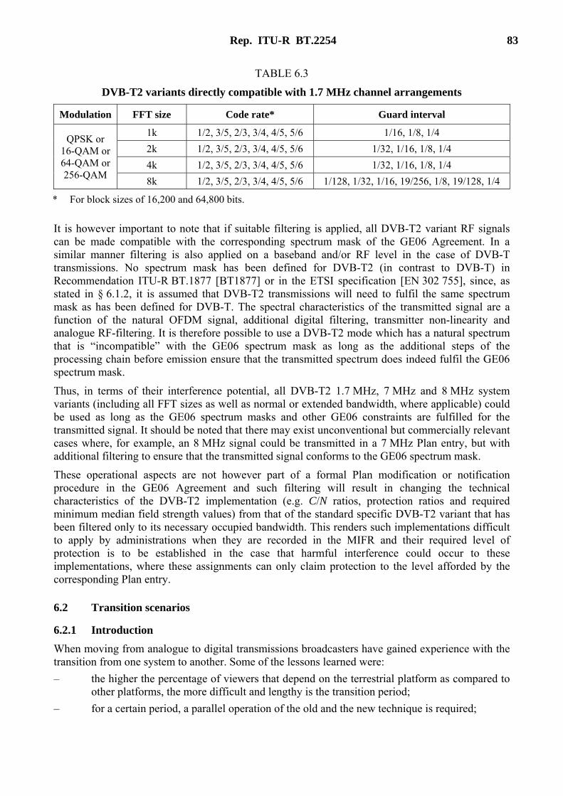
Rep. ITU-R BT.2254 83
TABLE 6.3
DVB-T2 variants directly compatible with 1.7 MHz channel arrangements
Modulation FFT size Code rate* Guard interval
QPSK or 16-QAM or 64-QAM or 256-QAM
1k 1/2, 3/5, 2/3, 3/4, 4/5, 5/6 1/16, 1/8, 1/4
2k 1/2, 3/5, 2/3, 3/4, 4/5, 5/6 1/32, 1/16, 1/8, 1/4
4k 1/2, 3/5, 2/3, 3/4, 4/5, 5/6 1/32, 1/16, 1/8, 1/4
8k 1/2, 3/5, 2/3, 3/4, 4/5, 5/6 1/128, 1/32, 1/16, 19/256, 1/8, 19/128, 1/4
* For block sizes of 16,200 and 64,800 bits.
It is however important to note that if suitable filtering is applied, all DVB-T2 variant RF signals can be made compatible with the corresponding spectrum mask of the GE06 Agreement. In a similar manner filtering is also applied on a baseband and/or RF level in the case of DVB-T transmissions. No spectrum mask has been defined for DVB-T2 (in contrast to DVB-T) in Recommendation ITU-R BT.1877 [BT1877] or in the ETSI specification [EN 302 755], since, as stated in § 6.1.2, it is assumed that DVB-T2 transmissions will need to fulfil the same spectrum mask as has been defined for DVB-T. The spectral characteristics of the transmitted signal are a function of the natural OFDM signal, additional digital filtering, transmitter non-linearity and analogue RF-filtering. It is therefore possible to use a DVB-T2 mode which has a natural spectrum that is “incompatible” with the GE06 spectrum mask as long as the additional steps of the processing chain before emission ensure that the transmitted spectrum does indeed fulfil the GE06 spectrum mask.
Thus, in terms of their interference potential, all DVB-T2 1.7 MHz, 7 MHz and 8 MHz system variants (including all FFT sizes as well as normal or extended bandwidth, where applicable) could be used as long as the GE06 spectrum masks and other GE06 constraints are fulfilled for the transmitted signal. It should be noted that there may exist unconventional but commercially relevant cases where, for example, an 8 MHz signal could be transmitted in a 7 MHz Plan entry, but with additional filtering to ensure that the transmitted signal conforms to the GE06 spectrum mask.
These operational aspects are not however part of a formal Plan modification or notification procedure in the GE06 Agreement and such filtering will result in changing the technical characteristics of the DVB-T2 implementation (e.g. C/N ratios, protection ratios and required minimum median field strength values) from that of the standard specific DVB-T2 variant that has been filtered only to its necessary occupied bandwidth. This renders such implementations difficult to apply by administrations when they are recorded in the MIFR and their required level of protection is to be established in the case that harmful interference could occur to these implementations, where these assignments can only claim protection to the level afforded by the corresponding Plan entry.
6.2 Transition scenarios
6.2.1 Introduction
When moving from analogue to digital transmissions broadcasters have gained experience with the transition from one system to another. Some of the lessons learned were:
– the higher the percentage of viewers that depend on the terrestrial platform as compared to other platforms, the more difficult and lengthy is the transition period;
– for a certain period, a parallel operation of the old and the new technique is required;
84 Rep. ITU-R BT.2254
– a certain amount of additional spectrum is needed for this, to accomplish the transition to new and more efficient techniques;
– an incentive in terms of additional programmes, higher service quality, etc. is required for viewers to accept the transition to new techniques because it may imply an upgrade of the user equipment, which they will have to pay for.
Some of these aspects are addressed further in this section as far as general considerations on the transition to DVB-T2 are concerned. Aspects particular to individual countries are described in Annex 6.
6.2.2 Infrastructure
For DVB-T2 the existing infrastructure (from analogue TV or DVB-T) which is related to antennas, masts, amplifiers, repeaters (although not re-transmitters which re-generate the signal), etc. at the transmitting side can be used. On the receiver side existing antenna infrastructure can be reused. This is valid if no change in the channel arrangement is made.
Since DVB-T2 is not downward compatible with DVB-T new tuners, i.e. new TV sets or at least additional set-top boxes are required at the receiving side. Accordingly, modulators, gateways in the case of SFNs, upgrade of the contribution network, monitoring equipment and possibly filters are required at the transmitting side. In addition, the operation modus of relays which are fed off-air may have to be changed with the migration to DVB-T2.
Most probably, also MPEG-4 source coding will then be used, although this aspect does not affect the RF transmission/reception side.
6.2.3 Frequency planning issues
The commercial requirements for DVB-T2 foresee compatibility with the GE06 Plan as a matter of principle. Therefore it is possible to use the existing GE06 Plan assignments and/or allotments for the implementation of DVB-T2. The preceding § 6.1 showed that there certain constraints have to be taken into account.
From a frequency planning point of view, for the transition to DVB-T2, it is therefore the easiest way to use the existing GE06 Plan structure. No additional frequency re-planning is required in this case, neither on national nor on international level. It implies that the same characteristics with regard to transmitter power, antenna position and diagram, etc. are used. A gain in data capacity and/or coverage quality is achieved. Similarly, for an allotment implementation the characteristics of the allotment plan entry regarding its interference potential should be kept while achieving a gain in data capacity and/or coverage quality.
But DVB-T2 would, in principle, also allow for a more radical approach with regard to frequency and network planning resulting in even higher spectrum efficiency. For DVB-T it is well known that the size of SFN is restricted because of self-interference effects. This restriction is reduced with DVB-T2 because of the larger guard intervals coming along with higher FFT modes. In a similar manner, existing coverage concepts (with regard to data capacity and reception mode) could be realized with less transmitter sites and/or frequency assignments.
But such approaches would imply a major re-arrangement of the existing frequency plan which is best achieved by a new planning conference. At present, such a general re-design of the existing frequency plan is not regarded as feasible. However, some improvements may be achieved by national or bilateral re-arrangements. An example for the latter is the aggregation of several national co-channel allotments to one large allotment in order to increase the coverage area which becomes technically possible with the new DVB-T2 variants; although then some multiplex capacity is lost.
Rep. ITU-R BT.2254 85
6.2.4 Transition from Analogue TV to DVB-T2
For countries that have not yet started their transition to DTT, it seems logical that they should immediately introduce DVB-T2. Since DVB-T2 has already started as a regular service in some countries it can be expected that DVB-T2 equipment will soon be available on a mass market.
It is expected that a simulcast period similar to that required for the transition from analogue TV to DVB-T will be needed for this transition. The length of the simulcast period will largely depend on the relevance of the terrestrial platform as compared to other platforms. The higher the terrestrial penetration the more care that needs to be taken with the transition, and in general, the more time it will take.
For the simulcast period, additional spectrum is required for the parallel transmission of TV services. The required amount of spectrum will heavily depend on the introduction strategy adopted for DVB-T2. For example in Spain, with a high percentage of the population using the terrestrial platform as their main means of reception, additional available spectrum was used for the simulcast period.
A short simulcast period will reduce additional costs, where possible a region-wise transition may avoid too abrupt changes across the whole country. This approach was taken by Germany with the introduction of DTT, based on the fact that the percentage of the terrestrial platform was relatively small.
The simulcast situation is eased with a transition from analogue to DVB-T2 as this technology can accommodate more individual programmes in a multiplex and so a smaller number of multiplexes is required. This will alleviate the cost of the simulcast period and the difficulty of finding spectrum for the simulcast.
6.2.5 Transition from DVB-T to DVB-T2
Many European countries have already introduced DVB-T and have, or are about to cease analogue transmissions. For them a migration to DVB-T2 is a possible next step in the development and implementation of broadcast delivery technologies.
DVB-T2 is not backwards compatible with DVB-T, so an abrupt migration from DVB-T to DVB-T2 is not possible. More sophisticated migration strategies are required. It is a commonly held view that this migration should be based on there being additional offers to the consumer in order to be successful. These offers may consist of additional programmes or may consist of different service types, such as HDTV.
In general therefore, for the migration period, unused and/or additional spectrum is required. This may be found in temporarily unused spectrum, available perhaps in countries where DVB-H is regarded as not being successful. Other countries may use available VHF spectrum for this purpose. A further possibility may be the more compact aggregation of DVB-T programmes in existing multiplexes (with a possible slight loss of quality) in order to free spectrum for an additional DVB-T2 multiplex. In exceptional cases the switch-off of DVB-T programmes may also be considered in order to free up spectrum for a DVB-T2 multiplex.
Some broadcasters may choose the enlarged possibilities of DVB-T2 to change or extend their coverage and/or service concept. For example, a change from a coverage which up to now mainly provides fixed reception to portable outdoor/mobile reception is possible. Also the provision of a better video quality is possible.
For countries that have already switched to DTT the issue of consumer reinvestment becomes an issue. The introduction of DVB-T, perhaps within the last ten years, was accompanied by the need for consumers to invest in new receiving equipment. Now, with the migration to DVB-T2, a new investment in receiving equipment is required by the consumers. This is a difficult situation since
86 Rep. ITU-R BT.2254
consumers have been used to longer renewal cycles of TV receiving equipment. The introductory strategy for DVB-T2 has to be chosen carefully in order not to lose customers to other platforms, as happened in some countries with the transition from Analogue TV to DVB-T.
A special situation arises in countries that have started but not completed the process of digital switch-over from Analogue TV to DVB-T and that also start to introduce DVB-T2. This situation is not that uncommon. Countries where the terrestrial platform is used by a large percentage of the population as the primary means of reception will necessarily have a long transition period and they are now faced with the challenge of an additional migration. Special considerations have then to be applied. A particular case is described in detail in Annex 6 for the United Kingdom.
7 References
[A122] DVB BlueBook A122 Rev.1, “Frame structure channel coding and modulation for a second generation digital terrestrial television broadcasting system (DVB-T2)”, DVB, January 2008.
[A133] DVB BlueBook A133, “Implementation guidelines for a second generation digital terrestrial television broadcasting system (DVB-T2)”, DVB, February 2009.
[A136] DVB Doc. A 136, “Modulator Interface (T2-MI) for a second generation digital terrestrial television broadcasting system (DVB-T2)”, DVB, February 2009.
[A150] DVB Doc. A 150, “Structure and modulation of optional transmitter signatures (T2-TX-SIG) for use with the DVB-T2”, DVB, June 2010.
[AFM2010] AFM-Report (ARD/ZDF), “Rundfunkrelevante Aspekte der Funkübertragungssysteme DVB-T2 und LTE“, ARD/ZDF, April 2010.
[BCP078] EBU Doc. B/BCP 078, “Man-Made Noise in the VHF- and UHF-Frequency Band: Results of Indoor Measurements”, Contribution from IRT, EBU, Geneva, 2005.
[BG2009] Brugger, R., Gbenga-Ilori, A., “Spectrum usage and requirements for future terrestrial broadcast applications” EBU Tech. Rev. 4/2009, EBU, Geneva, 2009.
[BH2003] Brugger, R., Hemmingway, D., “OFDM receivers – impact on coverage of inter-symbol interference and FFT window positioning”, EBU Tech.Rev. 295, EBU, Geneva, 2003.
[BPN005] EBU BPN005 3rd issue, “Terrestrial Digital Television – Planning and Implementation Considerations”, EBU, Geneva, 2001.
[BT1877] Recommendation ITU-R BT.1877, “Error-correction, data framing, modulation and emission methods for second generation of digital terrestrial television broadcasting systems”, ITU-R, Geneva, 2010.
[CPRT008] EBU Doc. CPRT 008 Rev1, “Proposed revision of planning criteria and parameter values given in EBU documents”, EBU, Geneva, 2004.
[ECC148] CEPT ECC Report 148, “Measurements on the performance of DVB-T receivers in the presence of interference from the mobile service (especially from LTE)”, CEPT, Copenhagen, 2010.
[ECC049] CEPT ECC Report 049, Annex 3, “Planning Configurations and Reference Networks for DVB-T”, CEPT, Copenhagen, 2004.
[EDP089] EBU Doc. ECS-EDP 089, “Symbol length and degradation beyond guard interval”, Contribution from IRT, EBU, Geneva, 2010.
[EDP135] EBU Doc. SM-EDP 135, “DVB-T2 THRESHOLDS- DATA FROM FIELD TRIALS”, contribution from University of the Basque Country (UPV/EHU), EBU, Geneva, 2011 also: Eizmendi, I, et al., CNR requirements for DVB-T2 fixed reception based on field trial results, Electronics Letters Volume: 47 Issue: 1, Jan. 2011.
Rep. ITU-R BT.2254 87
[EDP166] EBU Doc. SM-EDP 166, “C/N Measurements of DVB-T2 Receivers”, Contribution from IRT, EBU, Geneva, 2011.
[EDP-T7] EBU Doc. SM-EDP T7/Nov. 2010, “Implementation margin for C/N in DVB-T2”, Contribution from Teracom, EBU, Geneva, 2010.
[Ei2010] Eizmendi, I., et al., HDTV field trials using DVB-T and DVB-T2 broadcasting systems, 2010 IEEE International Symposium on Broadband Multimedia Systems and Broadcasting (BMSB).
[Ei2011] Eizmendi, I., PhD Thesis, Study of Minimum Requirements for DVB-T2 Digital Terrestrial System Fixed Reception, (in Spanish: Estudio de Requisitos Mínimos para la Recepción Fija del Sistema de Televisión Digital Terrestre DVB-T2). December 2011.
[EN 300 744] ETSI EN 300 744 V1.6.1 (2009-01), “Digital Video Broadcasting (DVB); Framing structure, channel coding and modulation for digital terrestrial television”, ETSI, Sophia Antipolis, 2009.
[EN 300 468] ETSI EN 300 468 V1.11.1 (2010-04) European Standard (Telecommunications series) Digital Video Broadcasting (DVB); Specification for Service Information (SI) in DVB systems, ETSI 2010.
[EN 302 307] ETSI EN 302 307 V1.2.1 (2009-08) “Digital Video Broadcasting (DVB); Second generation framing structure, channel coding and modulation systems for Broadcasting, Interactive Services”, News Gathering and other broadband satellite applications (DVB-S2).
[EN 302 755] ETSI EN 302 755 V1.2.1 (2011-02), “Digital Video Broadcasting (DVB); Frame structure channel coding and modulation for a second generation digital terrestrial television broadcasting system (DVB-T2)”, ETSI, Sophia Antipolis, 2011.
[EN 302 755-V1.3.1] ETSI EN 302 755 V1.3.1 (2011-11), “Digital Video Broadcasting (DVB); Frame structure channel coding and modulation for a second generation digital terrestrial television broadcasting system (DVB-T2)”, ETSI, Sophia Antipolis, 2011.
[EPB2011] Eizmendi, I.; Prieto, G.; Berjon-Eriz, G.; Velez, M.M.; Arrinda, A.; Angueira, P.; “DVB-T2 performance in presence of multipath laboratory tests,” Broadband Multimedia Systems and Broadcasting (BMSB), 2011 IEEE International Symposium pp. 1-6, 8-10 June 2011.
[F2010] Fischer, W., “Digital Video and Audio Broadcasting Technology: A Practical Engineering Guide”, Springer, Berlin, 2010.
[IEC 62216] IEC 62216 ed1.0, “Digital terrestrial television receivers for the DVB-T system”, IEC, 2009.
[IRT-2011-1] Pfeffer, R., IRT, private communication, 2011.
[IRT-2011-2] Beier, A., IRT, private communication, 2011.
[KHM1998] Kostanic, I., Hall, C., McCarthy, J., “Measurements of the vehicle penetration loss characteristics at 800 MHz”, Vehicular Technology Conference, 1998. VTC 98. pp. 1-4, IEEE, 1998.
[ND2007] Nour, C.A., Douillard, C., “Doubled diversity BICM schemes suitable for the DVB-T2 baseline”, ENST Bretagne, 2007.
[ND2008] Nour, C.A., Douillard, C., “Rotated-QAM Constellations to Improve BICM Performance for DVB-T2”, IEEE 10th Int. Symp. On Spread Spectrum Techniques and Applications, ISSSTA’08, p. 354, Bologna, 2008.
[NorDig2010] NorDig Unified Requirements for Integrated Receiver Decoders for use in cable, satellite, terrestrial and IP-based networks, NorDig Std. NorDig Unified ver 2.2.1, Dec. 2010.
88 Rep. ITU-R BT.2254
[NTIA02-390] Achatz, R.J., Dalke, R.A., “Man-Made Noise Power Measurements at VHF and UHF Frequencies”, NTIA Report 02 390, Boulder, December 2001.
[P372] Recommendation ITU-R P.372-10, “Radio Noise”, ITU-R, Geneva, 2009.
[P1546] Recommendation ITU-R P.1546-4, “Method for point-to-area predictions for terrestrial services in the frequency range 30 MHz to 3 000 MHz”, ITU-R, Geneva, 2009.
[Po2005] Poole, R., “Digital television services: Equivalent noise floors and equivalent noise degradation,” BBC R&D, White Paper WHP 105, January, 2005.
[Ro2009] Robert, J., “Präsentation DVB-T2 Sendernetzplanung”, Institut für Nachrichtentechnik TU-Braunschweig, March 2009.
[RRC04] RRC-04: “Report of the first session of the conference to the second session of the conference, chapter 3: Technical basis and characteristics”, ITU-R, Geneva, 2004.
[RRC06] RRC-06, “Final Acts of the Regional Radiocommunication Conference RRC-06, chapter 3 of Annex 2”, ITU-R, Geneva, 2006.
[SM1875] Recommendation ITU-R SM.1875, "DVB-T coverage measurements and verification of planning criteria", ITU-R, Geneva, 2010.
[St1998] Stott, J. H., “The effects of phase noise in COFDM”, EBU Technical Review, (276), pp. 12-25, Summer 1998 available from BBC website: http://www.bbc.co.uk/rd/pubs/papers/pdffiles/jsebu276.pdf.
[Tech3317] EBU Tech 3317, “Planning parameters for hand-held reception”, EBU, Geneva, 2007.
[TR 102 377] ETSI TR 102 377 V1.2.2 (2006-01), “Digital Video Broadcasting (DVB); DVB-H Implementation Guidelines”, ETSI, Sophia Antipolis, 2006.
[TS 102 773] ETSI TS 102 773 V1.3.1 (2012-01): Digital Video Broadcasting (DVB);Modulator Interface (T2-MI) for a second generation digital terrestrial television broadcasting system (DVB-T2), ETSI, 2012.
[TS 102 831] ETSI TS 102 831 V1.1.1 (2010-10), “Digital Video Broadcasting (DVB); Implementation guidelines for a second generation digital terrestrial television broadcasting system (DVB-T2)”, ETSI, Sophia Antipolis, 2010.
[WP6A-619] ITU-R WP6A Doc. 619, “Annex 9 to Working Party 6A Chairman’s Report. WORKING DOCUMENT TOWARDS A PRELIMINARY DRAFT NEW RECOMMENDATION ITU-R BT.[2NDDTTBPLAN]. Planning criteria, including protection ratios, for second generation of digital terrestrial television broadcasting systems in the VHF/UHF bands”. ITU-R, Geneva, 2011.
Rep. ITU-R BT.2254 89
Annex 1
Planning methods, criteria and parameter
A1.1 Reception modes
A1.1.1 Fixed antenna reception
Fixed antenna reception is defined as:
Reception where a directional receiving antenna mounted at roof-level is used. In calculating the equivalent field strength required for fixed antenna reception, a receiving antenna height of 10 m above ground level is considered to be representative.
A1.1.2 Portable antenna reception
In the context of this document, portable reception is defined as the reception at rest (stationary reception) or at very low speed (walking speed). Portable reception will, in practice, take place under a great variety of conditions (outdoor, indoor, ground floor and upper floors). In this document, portable reception is comprised of two classes:
– Class A: portable outdoor reception
i) with external (for example telescopic or wired headsets) or integrated antenna;
ii) at no less than 1.5 m above ground level, at very low speed or at rest.
– Class B: portable indoor reception
i) with external (for example telescopic or wired headsets) or integrated antenna;
ii) at no less than 1.5 m above ground level, at very low speed or at rest;
iii) on the ground floor in a room with a window in an external wall.
It is assumed that the portable receiver is not moved during reception and that large objects near the receiver are also not moved. This does not mean that the transmission channel is static; rather, a slowly time-varying channel is assumed. It is also understood that extreme cases, such as reception in completely shielded rooms, be disregarded.
A1.1.3 Mobile reception
Mobile reception is defined as the reception of a DVB-T2 signal by a receiver in motion with an antenna situated at no less than 1.5 m above ground level. The term motion covers speeds from a walking person to a car driven on a motorway. High-speed trains, buses and other vehicles could be considered in some countries.
A1.1.4 Handheld reception
A1.1.4.1 Handheld portable reception
In the context of this document, handheld portable reception is defined as the reception at rest (stationary reception) or at very low speed (walking speed). Handheld portable reception will, in practice, take place under a great variety of conditions (outdoor, indoor, ground floor and upper floors). In addition, the handheld receiver will probably be moved (at walking speed) while being viewed.
The difference between portable reception and handheld portable reception lies in the different antenna gains which are assumed for the two reception modes.
90 Rep. ITU-R BT.2254
In this document, handheld portable reception is comprised of two classes:
– Class H-A: handheld portable outdoor reception
i) with external (for example telescopic or wired headsets) or integrated antenna;
ii) at no less than 1.5 m above ground level, at very low speed or at rest.
– Class H-B: handheld portable indoor reception
i) with external (for example telescopic or wired headsets) or integrated antenna;
ii) at no less than 1.5 m above ground level, at very low speed or at rest;
iii) on the ground floor in a room with a window in an external wall.
It is assumed that the handheld portable receiver is not moved during reception and that large objects near the receiver are also not moved. This does not mean that the transmission channel is static; rather, a slowly time-varying channel is assumed. It is also understood that extreme cases, such as reception in completely shielded rooms, be disregarded.
For the handheld reception mode, it is often possible to improve reception by moving the receiver position and/or by using an antenna with higher efficiency.
It is to be expected that there will be significant variation of reception conditions for indoor portable reception, also depending on the floor-level at which reception is required. There will also be considerable variation of building penetration loss from one building to another and considerable variation from one part of a room to another. Also, handheld receivers could suffer from body-absorption/reflection loss in certain circumstances, e.g. file-downloading applications when the receiver is in a pocket. It is to be expected that “portable coverage” will be mainly aimed at urban and suburban areas.
A1.1.4.2 Handheld mobile reception
In the context of this document, handheld mobile reception is comprised of two classes:
– Class H-C: handheld reception inside a moving vehicle (car, bus, etc.)
i) with the receiver connected to the external antenna of the vehicle;
ii) at no less than 1.5 m above ground level, at higher speed.
– Class H-D: handheld reception inside a moving vehicle (e.g. car, bus, etc.)
i) without connexion of the receiver to the external antenna of the vehicle;
ii) with external (for example telescopic or wired headsets) or integrated antenna;
iii) at no less than 1.5 m above ground level, at higher speed.
It should be noted that body-absorption/reflection losses could also be of importance in Class H-D under certain circumstances, for example when the terminal is in a pocket and file downloading is under way. However, this document does not consider this situation.
It is to be expected that there will be significant variation of reception conditions for handheld mobile reception, depending on the environment of the receiver. There might also be considerable variation of entry loss caused by the varying construction of cars and vehicles.
In both cases, it is assumed that the handheld mobile receiver and/or large objects near the receiver may move during the reception. It is also understood that extreme cases, such as reception in completely shielded vehicles, be disregarded.
Again, the difference between mobile reception and handheld mobile reception, Class H-C, lies in the different antenna gains which are assumed for the two reception modes.
Rep. ITU-R BT.2254 91
A1.2 Coverage definitions
It is necessary to have definitions for the coverage of a terrestrial television transmitting station or a group of such stations. Digital television service coverage is characterized by a very rapid transition from near perfect reception to no reception at all and it thus becomes critical to be able to define which areas are going to be covered and which are not. However, because of the very rapid transition described above, there is a cost penalty if the coverage target within a small area (say, 100 m × 100 m) is set too high. This occurs because it is necessary either to increase the transmitter powers or to provide a larger number of transmitters in order to guarantee coverage to the last few percent of the worst-served small areas.
For this reason, the coverage definition of “good” has been selected as the case where 95% of the locations within a small area are covered. Similarly, “acceptable” has been defined to be the case where 70% of the locations within a small area are covered.
The definitions do not aim to describe the area where coverage is achieved under worst-case conditions. They provide a description of the area where “good” or “acceptable” coverage should be achieved under representative practical conditions. They may be regarded as describing the “quality” of the coverage achieved.
In defining the coverage area for each reception condition, a three-level approach is taken:
Receiving location
The smallest unit is a receiving location with dimensions of about 0.5 m × 0.5 m. In the case of portable antenna reception, it is assumed that optimal receiving conditions will be found by moving the antenna or by moving the handheld terminal up to 0.5 m in any direction.
Such a location is regarded as covered if the required carrier-to-noise and carrier-to-interference values are achieved for 99% of the time.
Small area coverage
The second level is a “small area” (typically 100 m × 100 m). In this small area the percentage of covered location is indicated.
The coverage of a small area is classified as:
– “Good”, if at least 95% of receiving locations within the area are covered for portable reception and 99% of receiving locations within it are covered for mobile reception.
– “Acceptable”, if at least 70% of receiving locations within the area are covered for portable reception and 90% of receiving locations within it are covered for mobile reception.
Coverage area
The third level is the coverage area.
The coverage area of a transmitter, or a group of transmitters, is made up of the sum of the individual small areas in which a given class of coverage is achieved.
A1.3 Calculation of signal levels
To calculate the minimum median power flux-density or equivalent field strength needed to ensure that the minimum values of signal level can be achieved at the required percentage of locations, the following formulas are used:
φmin = Ps min – Aa + Lf
Emin = φmin + 120 + 10 log10 (120 π) = φmin + 145.8

92 Rep. ITU-R BT.2254
φmed = φmin + Pmmn + Cl (for fixed reception)
φmed = φmin + Pmmn + Cl + Lh (for portable outdoor reception, Class A, mobile reception and, handheld portable outdoor reception, Class H-A, and handheld mobile vehicular reception, Class H-C)
φmed = φmin + Pmmn + Cl + Lh + Lb (for portable indoor reception, Class B, and handheld portable indoor reception, Class H-B)
φmed = φmin + Pmmn + Cl + Lh + Lv (for handheld mobile reception, Class H-D)
Emed = φmed + 120 + 10 log10 (120 π) = φmed + 145.8
where:
C/N: RF signal-to-noise ratio required by the system (dB)
φmin: Minimum power flux-density at receiving place (dBW/m2)
Emin: Equivalent minimum field strength at receiving place (dBμV/m)
Lf: Feeder loss (dB)
Lh: Height loss (10 m a.g.l. to 1.5 m a.g.l.) (dB)
Lb: Building penetration loss (dB)
Lv: Vehicle entry loss (dB)
Pmmn: Allowance for man-made noise (dB)
Cl: Location correction factor (dB)
φmed: Minimum median power flux-density, planning value (dBW/m2)
Emed: Minimum median equivalent field strength, planning value (dBμV/m)
Aa: Effective antenna aperture (dBm2) (Aa = Giso + 10log10(λ2/4π)). Giso is the antenna gain relative to an isotropic antenna
Ps min: Minimum receiver input power (dBW)
For calculating the location correction factor Cl a log-normal distribution of the received signal is assumed.
Cl = μ * σ
where:
μ: distribution factor, being 0.52 for 70%, 1.28 for 90%, 1.64 for 95% and 2.33 for 99%;
σ: standard deviation taken as 5.5 dB for outdoor reception. See § A1.3.7 for σ values appropriate for indoor reception.
While the matters dealt with in this section are generally applicable, additional special considerations are needed in the case of SFNs where there is more than one wanted signal contribution.
Rep. ITU-R BT.2254 93
A1.3.1 Antenna gain
The antenna gains used in the derivation of the minimum median wanted signal levels in § 3 are given in Table A1.1.
For portable and mobile reception, an omnidirectional antenna is applied.
Within any frequency band, the variation of antenna gain with frequency may be taken into account by the addition of a correction term:
Corr = 10 log10(FA/FR)
where:
FA: actual frequency being considered;
FR: relevant reference frequency quoted in § 3.
For further detailed information concerning the antenna gain values of handheld receivers, see § 1.3.3.2 of [Tech3317].
TABLE A1.1
Antenna gain in dBd for the different bands and for the different reception modes
Gain (dBd)
Reception Mode Band III
Bands IV/V
Rooftop antenna 7 11 Fixed rooftop
Adapted antenna –2.2 0 Portable Class A and B Mobile Handheld mobile vehicular Class H-C
External antenna* –13 –5.5 Handheld portable outdoor Cass H-A Handheld portable indoor Cass H-B Handheld mobile reception H-D
Integrated antenna –17 –9.5 Handheld portable outdoor Cass H-A Handheld portable indoor Cass H-B Handheld mobile reception H-D
* Telescopic or wired headsets.
A1.3.2 Feeder loss
The feeder losses used in the derivation of the minimum median wanted signal levels in § 3 are given in Table A1.2:
TABLE A1.2
Feeder loss in dB for the different bands
Feeder loss (dB)
Band III Bands IV/V Reception Mode
Rooftop antenna 2 4 Fixed rooftop
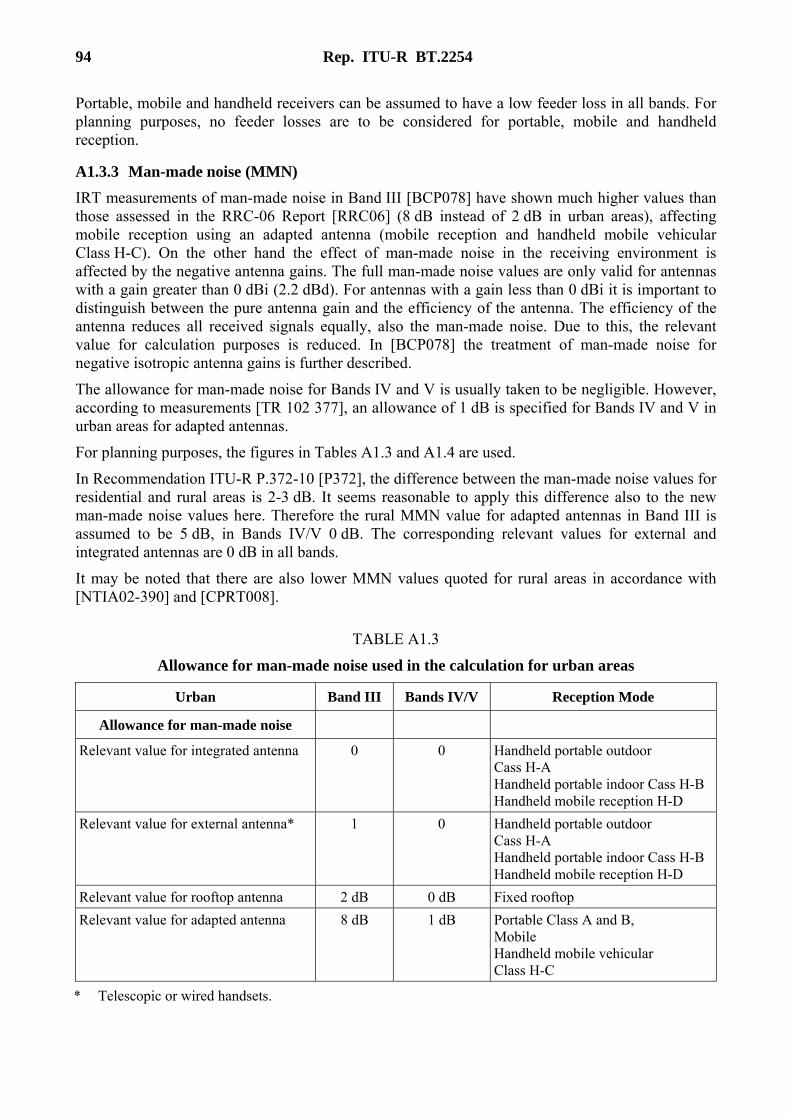
94 Rep. ITU-R BT.2254
Portable, mobile and handheld receivers can be assumed to have a low feeder loss in all bands. For planning purposes, no feeder losses are to be considered for portable, mobile and handheld reception.
A1.3.3 Man-made noise (MMN)
IRT measurements of man-made noise in Band III [BCP078] have shown much higher values than those assessed in the RRC-06 Report [RRC06] (8 dB instead of 2 dB in urban areas), affecting mobile reception using an adapted antenna (mobile reception and handheld mobile vehicular Class H-C). On the other hand the effect of man-made noise in the receiving environment is affected by the negative antenna gains. The full man-made noise values are only valid for antennas with a gain greater than 0 dBi (2.2 dBd). For antennas with a gain less than 0 dBi it is important to distinguish between the pure antenna gain and the efficiency of the antenna. The efficiency of the antenna reduces all received signals equally, also the man-made noise. Due to this, the relevant value for calculation purposes is reduced. In [BCP078] the treatment of man-made noise for negative isotropic antenna gains is further described.
The allowance for man-made noise for Bands IV and V is usually taken to be negligible. However, according to measurements [TR 102 377], an allowance of 1 dB is specified for Bands IV and V in urban areas for adapted antennas.
For planning purposes, the figures in Tables A1.3 and A1.4 are used.
In Recommendation ITU-R P.372-10 [P372], the difference between the man-made noise values for residential and rural areas is 2-3 dB. It seems reasonable to apply this difference also to the new man-made noise values here. Therefore the rural MMN value for adapted antennas in Band III is assumed to be 5 dB, in Bands IV/V 0 dB. The corresponding relevant values for external and integrated antennas are 0 dB in all bands.
It may be noted that there are also lower MMN values quoted for rural areas in accordance with [NTIA02-390] and [CPRT008].
TABLE A1.3
Allowance for man-made noise used in the calculation for urban areas
Urban Band III Bands IV/V Reception Mode
Allowance for man-made noise
Relevant value for integrated antenna 0 0 Handheld portable outdoor Cass H-A Handheld portable indoor Cass H-BHandheld mobile reception H-D
Relevant value for external antenna* 1 0 Handheld portable outdoor Cass H-A Handheld portable indoor Cass H-BHandheld mobile reception H-D
Relevant value for rooftop antenna 2 dB 0 dB Fixed rooftop
Relevant value for adapted antenna 8 dB 1 dB Portable Class A and B, Mobile Handheld mobile vehicular Class H-C
* Telescopic or wired handsets.
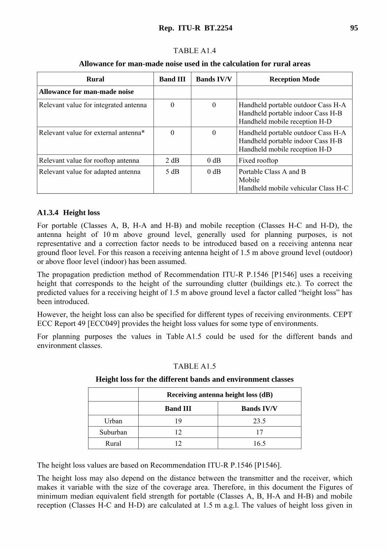
Rep. ITU-R BT.2254 95
TABLE A1.4
Allowance for man-made noise used in the calculation for rural areas
Rural Band III Bands IV/V Reception Mode
Allowance for man-made noise
Relevant value for integrated antenna 0 0 Handheld portable outdoor Cass H-A Handheld portable indoor Cass H-B Handheld mobile reception H-D
Relevant value for external antenna* 0 0 Handheld portable outdoor Cass H-A Handheld portable indoor Cass H-B Handheld mobile reception H-D
Relevant value for rooftop antenna 2 dB 0 dB Fixed rooftop
Relevant value for adapted antenna 5 dB 0 dB Portable Class A and B Mobile Handheld mobile vehicular Class H-C
A1.3.4 Height loss
For portable (Classes A, B, H-A and H-B) and mobile reception (Classes H-C and H-D), the antenna height of 10 m above ground level, generally used for planning purposes, is not representative and a correction factor needs to be introduced based on a receiving antenna near ground floor level. For this reason a receiving antenna height of 1.5 m above ground level (outdoor) or above floor level (indoor) has been assumed.
The propagation prediction method of Recommendation ITU-R P.1546 [P1546] uses a receiving height that corresponds to the height of the surrounding clutter (buildings etc.). To correct the predicted values for a receiving height of 1.5 m above ground level a factor called “height loss” has been introduced.
However, the height loss can also be specified for different types of receiving environments. CEPT ECC Report 49 [ECC049] provides the height loss values for some type of environments.
For planning purposes the values in Table A1.5 could be used for the different bands and environment classes.
TABLE A1.5
Height loss for the different bands and environment classes
Receiving antenna height loss (dB)
Band III Bands IV/V
Urban 19 23.5
Suburban 12 17
Rural 12 16.5
The height loss values are based on Recommendation ITU-R P.1546 [P1546].
The height loss may also depend on the distance between the transmitter and the receiver, which makes it variable with the size of the coverage area. Therefore, in this document the Figures of minimum median equivalent field strength for portable (Classes A, B, H-A and H-B) and mobile reception (Classes H-C and H-D) are calculated at 1.5 m a.g.l. The values of height loss given in
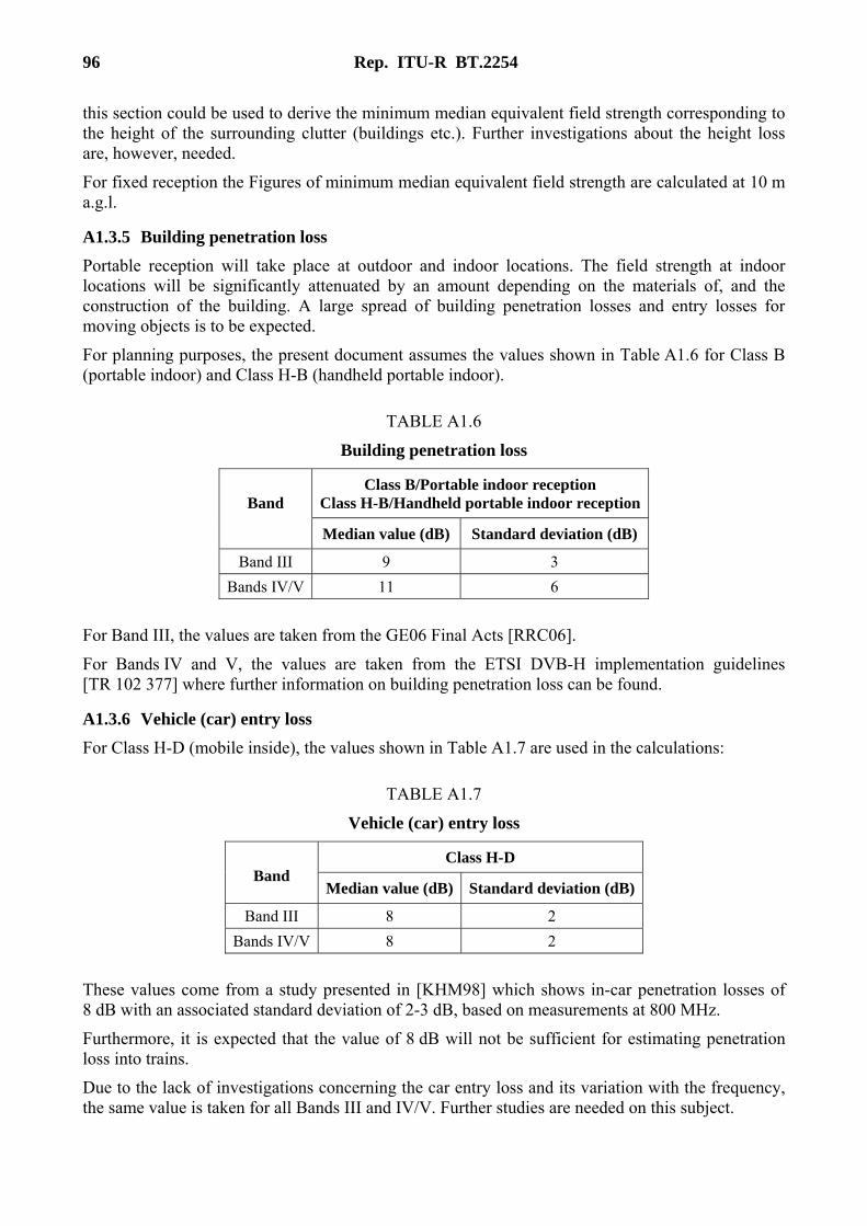
96 Rep. ITU-R BT.2254
this section could be used to derive the minimum median equivalent field strength corresponding to the height of the surrounding clutter (buildings etc.). Further investigations about the height loss are, however, needed.
For fixed reception the Figures of minimum median equivalent field strength are calculated at 10 m a.g.l.
A1.3.5 Building penetration loss
Portable reception will take place at outdoor and indoor locations. The field strength at indoor locations will be significantly attenuated by an amount depending on the materials of, and the construction of the building. A large spread of building penetration losses and entry losses for moving objects is to be expected.
For planning purposes, the present document assumes the values shown in Table A1.6 for Class B (portable indoor) and Class H-B (handheld portable indoor).
TABLE A1.6
Building penetration loss
Band
Class B/Portable indoor reception Class H-B/Handheld portable indoor reception
Median value (dB) Standard deviation (dB)
Band III 9 3
Bands IV/V 11 6
For Band III, the values are taken from the GE06 Final Acts [RRC06].
For Bands IV and V, the values are taken from the ETSI DVB-H implementation guidelines [TR 102 377] where further information on building penetration loss can be found.
A1.3.6 Vehicle (car) entry loss
For Class H-D (mobile inside), the values shown in Table A1.7 are used in the calculations:
TABLE A1.7
Vehicle (car) entry loss
Band
Class H-D
Median value (dB) Standard deviation (dB)
Band III 8 2
Bands IV/V 8 2
These values come from a study presented in [KHM98] which shows in-car penetration losses of 8 dB with an associated standard deviation of 2-3 dB, based on measurements at 800 MHz.
Furthermore, it is expected that the value of 8 dB will not be sufficient for estimating penetration loss into trains.
Due to the lack of investigations concerning the car entry loss and its variation with the frequency, the same value is taken for all Bands III and IV/V. Further studies are needed on this subject.
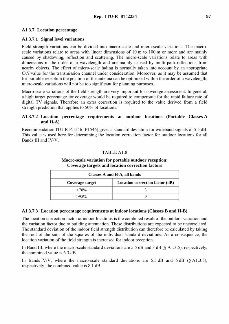
Rep. ITU-R BT.2254 97
A1.3.7 Location percentage
A1.3.7.1 Signal level variations
Field strength variations can be divided into macro-scale and micro-scale variations. The macro-scale variations relate to areas with linear dimensions of 10 m to 100 m or more and are mainly caused by shadowing, reflection and scattering. The micro-scale variations relate to areas with dimensions in the order of a wavelength and are mainly caused by multi-path reflections from nearby objects. The effect of micro-scale fading is normally taken into account by an appropriate C/N value for the transmission channel under consideration. Moreover, as it may be assumed that for portable reception the position of the antenna can be optimized within the order of a wavelength, micro-scale variations will not be too significant for planning purposes.
Macro-scale variations of the field strength are very important for coverage assessment. In general, a high target percentage for coverage would be required to compensate for the rapid failure rate of digital TV signals. Therefore an extra correction is required to the value derived from a field strength prediction that applies to 50% of locations.
A1.3.7.2 Location percentage requirements at outdoor locations (Portable Classes A and H-A)
Recommendation ITU-R P.1546 [P1546] gives a standard deviation for wideband signals of 5.5 dB. This value is used here for determining the location correction factor for outdoor locations for all Bands III and IV/V.
TABLE A1.8
Macro-scale variation for portable outdoor reception: Coverage targets and location correction factors
Classes A and H-A, all bands
Coverage target Location correction factor (dB)
>70% 3
>95% 9
A1.3.7.3 Location percentage requirements at indoor locations (Classes B and H-B)
The location correction factor at indoor locations is the combined result of the outdoor variation and the variation factor due to building attenuation. These distributions are expected to be uncorrelated. The standard deviation of the indoor field strength distribution can therefore be calculated by taking the root of the sum of the squares of the individual standard deviations. As a consequence, the location variation of the field strength is increased for indoor reception.
In Band III, where the macro-scale standard deviations are 5.5 dB and 3 dB (§ A1.3.5), respectively, the combined value is 6.3 dB.
In Bands IV/V, where the macro-scale standard deviations are 5.5 dB and 6 dB (§ A1.3.5), respectively, the combined value is 8.1 dB.
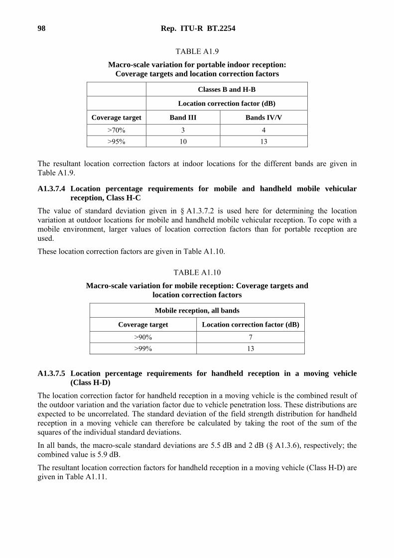
98 Rep. ITU-R BT.2254
TABLE A1.9
Macro-scale variation for portable indoor reception: Coverage targets and location correction factors
Classes B and H-B
Location correction factor (dB)
Coverage target Band III Bands IV/V
>70% 3 4
>95% 10 13
The resultant location correction factors at indoor locations for the different bands are given in Table A1.9.
A1.3.7.4 Location percentage requirements for mobile and handheld mobile vehicular reception, Class H-C
The value of standard deviation given in § A1.3.7.2 is used here for determining the location variation at outdoor locations for mobile and handheld mobile vehicular reception. To cope with a mobile environment, larger values of location correction factors than for portable reception are used.
These location correction factors are given in Table A1.10.
TABLE A1.10
Macro-scale variation for mobile reception: Coverage targets and location correction factors
Mobile reception, all bands
Coverage target Location correction factor (dB)
>90% 7
>99% 13
A1.3.7.5 Location percentage requirements for handheld reception in a moving vehicle (Class H-D)
The location correction factor for handheld reception in a moving vehicle is the combined result of the outdoor variation and the variation factor due to vehicle penetration loss. These distributions are expected to be uncorrelated. The standard deviation of the field strength distribution for handheld reception in a moving vehicle can therefore be calculated by taking the root of the sum of the squares of the individual standard deviations.
In all bands, the macro-scale standard deviations are 5.5 dB and 2 dB (§ A1.3.6), respectively; the combined value is 5.9 dB.
The resultant location correction factors for handheld reception in a moving vehicle (Class H-D) are given in Table A1.11.
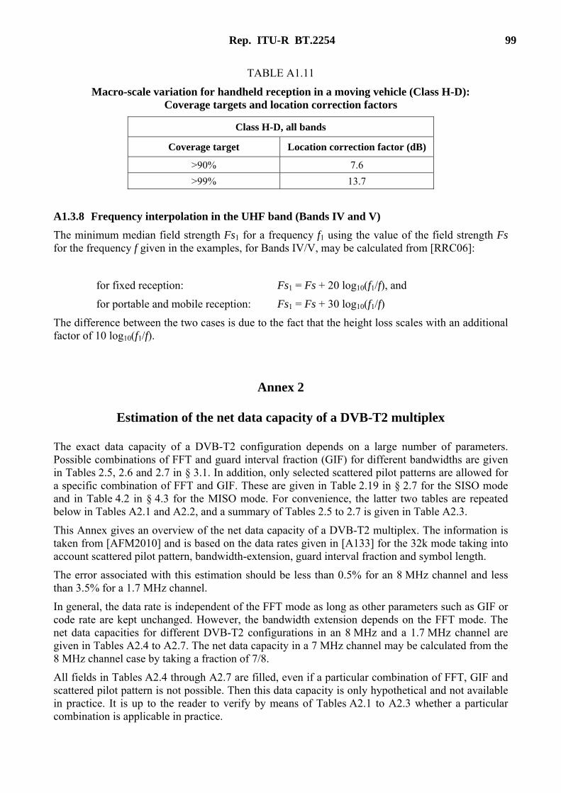
Rep. ITU-R BT.2254 99
TABLE A1.11
Macro-scale variation for handheld reception in a moving vehicle (Class H-D): Coverage targets and location correction factors
Class H-D, all bands
Coverage target Location correction factor (dB)
>90% 7.6
>99% 13.7
A1.3.8 Frequency interpolation in the UHF band (Bands IV and V)
The minimum median field strength Fs1 for a frequency f1 using the value of the field strength Fs for the frequency f given in the examples, for Bands IV/V, may be calculated from [RRC06]:
for fixed reception: Fs1 = Fs + 20 log10(f1/f), and
for portable and mobile reception: Fs1 = Fs + 30 log10(f1/f)
The difference between the two cases is due to the fact that the height loss scales with an additional factor of 10 log10(f1/f).
Annex 2
Estimation of the net data capacity of a DVB-T2 multiplex
The exact data capacity of a DVB-T2 configuration depends on a large number of parameters. Possible combinations of FFT and guard interval fraction (GIF) for different bandwidths are given in Tables 2.5, 2.6 and 2.7 in § 3.1. In addition, only selected scattered pilot patterns are allowed for a specific combination of FFT and GIF. These are given in Table 2.19 in § 2.7 for the SISO mode and in Table 4.2 in § 4.3 for the MISO mode. For convenience, the latter two tables are repeated below in Tables A2.1 and A2.2, and a summary of Tables 2.5 to 2.7 is given in Table A2.3.
This Annex gives an overview of the net data capacity of a DVB-T2 multiplex. The information is taken from [AFM2010] and is based on the data rates given in [A133] for the 32k mode taking into account scattered pilot pattern, bandwidth-extension, guard interval fraction and symbol length.
The error associated with this estimation should be less than 0.5% for an 8 MHz channel and less than 3.5% for a 1.7 MHz channel.
In general, the data rate is independent of the FFT mode as long as other parameters such as GIF or code rate are kept unchanged. However, the bandwidth extension depends on the FFT mode. The net data capacities for different DVB-T2 configurations in an 8 MHz and a 1.7 MHz channel are given in Tables A2.4 to A2.7. The net data capacity in a 7 MHz channel may be calculated from the 8 MHz channel case by taking a fraction of 7/8.
All fields in Tables A2.4 through A2.7 are filled, even if a particular combination of FFT, GIF and scattered pilot pattern is not possible. Then this data capacity is only hypothetical and not available in practice. It is up to the reader to verify by means of Tables A2.1 to A2.3 whether a particular combination is applicable in practice.
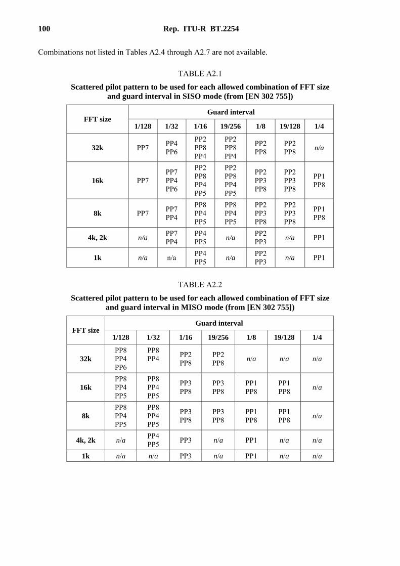
100 Rep. ITU-R BT.2254
Combinations not listed in Tables A2.4 through A2.7 are not available.
TABLE A2.1
Scattered pilot pattern to be used for each allowed combination of FFT size and guard interval in SISO mode (from [EN 302 755])
FFT size Guard interval
1/128 1/32 1/16 19/256 1/8 19/128 1/4
32k PP7 PP4 PP6
PP2 PP8 PP4
PP2 PP8 PP4
PP2 PP8
PP2 PP8
n/a
16k PP7 PP7 PP4 PP6
PP2 PP8 PP4 PP5
PP2 PP8 PP4 PP5
PP2 PP3 PP8
PP2 PP3 PP8
PP1 PP8
8k PP7 PP7 PP4
PP8 PP4 PP5
PP8 PP4 PP5
PP2 PP3 PP8
PP2 PP3 PP8
PP1 PP8
4k, 2k n/a PP7 PP4
PP4 PP5
n/a PP2 PP3
n/a PP1
1k n/a n/a PP4 PP5
n/a PP2 PP3
n/a PP1
TABLE A2.2
Scattered pilot pattern to be used for each allowed combination of FFT size and guard interval in MISO mode (from [EN 302 755])
FFT size Guard interval
1/128 1/32 1/16 19/256 1/8 19/128 1/4
32k PP8 PP4 PP6
PP8 PP4
PP2 PP8
PP2 PP8
n/a n/a n/a
16k PP8 PP4 PP5
PP8 PP4 PP5
PP3 PP8
PP3 PP8
PP1 PP8
PP1 PP8
n/a
8k PP8 PP4 PP5
PP8 PP4 PP5
PP3 PP8
PP3 PP8
PP1 PP8
PP1 PP8
n/a
4k, 2k n/a PP4 PP5
PP3 n/a PP1 n/a n/a
1k n/a n/a PP3 n/a PP1 n/a n/a

Rep. ITU-R BT.2254 101
TABLE A2.3
Allowed combinations of FFT and GIF
FFT GIF
1/128 1/32 1/16 19/256 1/8 19/128 1/4
32k Yes Yes Yes Yes Yes Yes No
16k Yes Yes Yes Yes Yes Yes Yes
8k Yes Yes Yes Yes Yes Yes Yes
4k No Yes Yes No Yes No No
2k No Yes Yes No Yes No No
1k No No Yes No Yes No No

102 Rep. ITU-R BT.2254
TABLE A2.4
Capacity in a 8 MHz channel, normal carrier mode, FFT modes: 1k to 32k
Scattered Pilot Pattern 1 & 2 Scattered Pilot Pattern 3 & 4
GIF GIF
Modulation Coderate
1/128 (Mbit/s)
1/32 (Mbit/s)
1/16 (Mbit/s)
19/256 (Mbit/s)
1/8 (Mbit/s)
19/128 (Mbit/s)
1/4 (Mbit/s)
1/128 (Mbit/s)
1/32 (Mbit/s)
1/16 (Mbit/s)
19/256 (Mbit/s)
1/8 (Mbit/s)
19/128 (Mbit/s)
1/4 (Mbit/s)
QPSK
1/2 6.8 6.6 6.5 6.4 6.1 6.0 5.5 7.1 6.9 6.7 6.7 6.4 6.2 5.7
3/5 8.2 8.0 7.8 7.7 7.3 7.2 6.6 8.5 8.3 8.1 8.0 7.7 7.5 6.9
2/3 9.1 8.9 8.6 8.5 8.2 8.0 7.3 9.5 9.3 9.0 8.9 8.5 8.3 7.7
3/4 10.2 10.0 9.7 9.6 9.2 9.0 8.3 10.7 10.4 10.1 10.0 9.6 9.4 8.6
4/5 10.9 10.7 10.4 10.2 9.8 9.6 8.8 11.4 11.1 10.8 10.7 10.2 10.0 9.2
5/6 11.4 11.1 10.8 10.7 10.2 10.0 9.2 11.9 11.6 11.3 11.2 10.7 10.4 9.6
16-QAM
1/2 13.6 13.3 12.9 12.8 12.2 12.0 11.0 14.3 13.9 13.5 13.4 12.8 12.5 11.5
3/5 16.4 16.0 15.6 15.4 14.7 14.4 13.2 17.1 16.7 16.3 16.1 15.4 15.1 13.8
2/3 18.2 17.8 17.3 17.1 16.4 16.0 14.7 19.1 18.6 18.1 17.9 17.1 16.7 15.4
3/4 20.5 20.1 19.5 19.3 18.4 18.0 16.6 21.4 21.0 20.4 20.1 19.2 18.8 17.3
4/5 21.9 21.4 20.8 20.6 19.6 19.2 17.7 22.9 22.4 21.7 21.5 20.5 20.1 18.5
5/6 22.8 22.3 21.7 21.4 20.5 20.1 18.4 23.9 23.3 22.6 22.4 21.4 21.0 19.3
64-QAM
1/2 20.4 20.0 19.4 19.2 18.3 18.0 16.5 21.4 20.9 20.3 20.0 19.1 18.8 17.2
3/5 24.6 24.0 23.3 23.1 22.0 21.6 19.8 25.7 25.1 24.4 24.1 23.0 22.5 20.7
2/3 27.3 26.7 25.9 25.7 24.5 24.0 22.1 28.6 27.9 27.1 26.8 25.6 25.1 23.1
3/4 30.7 30.0 29.2 28.9 27.6 27.0 24.8 32.1 31.4 30.5 30.2 28.8 28.2 25.9
4/5 32.8 32.1 31.1 30.8 29.4 28.8 26.5 34.3 33.5 32.5 32.2 30.7 30.1 27.7
5/6 34.2 33.4 32.5 32.1 30.7 30.0 27.6 35.7 34.9 33.9 33.5 32.0 31.4 28.9
256-QAM
1/2 27.3 26.7 25.9 25.6 24.5 24.0 22.1 28.5 27.9 27.1 26.8 25.6 25.1 23.0
3/5 32.8 32.1 31.1 30.8 29.4 28.8 26.5 34.3 33.5 32.5 32.2 30.7 30.1 27.7
2/3 36.5 35.7 34.6 34.3 32.7 32.1 29.5 38.1 37.3 36.2 35.8 34.2 33.5 30.8
3/4 41.1 40.1 39.0 38.6 36.8 36.1 33.2 42.9 41.9 40.7 40.3 38.5 37.7 34.7
4/5 43.8 42.8 41.6 41.1 39.3 38.5 35.4 45.8 44.8 43.5 43.0 41.1 40.2 37.0
5/6 45.7 44.7 43.4 42.9 41.0 40.1 36.9 47.7 46.7 45.3 44.8 42.8 41.9 38.6

Rep. ITU-R BT.2254 103
TABLE A2.4 (end)
Scattered Pilot Pattern 5 & 6 Scattered Pilot Pattern 7 & 8
GIF GIF
Modulation Code rate
1/128 (Mbit/s)
1/32 (Mbit/s)
1/16 (Mbit/s)
19/256 (Mbit/s)
1/8 (Mbit/s)
19/128 (Mbit/s)
1/4 (Mbit/s)
1/128 (Mbit/s)
1/32 (Mbit/s)
1/16 (Mbit/s)
19/256 (Mbit/s)
1/8 (Mbit/s)
19/128 (Mbit/s)
1/4 (Mbit/s)
QPSK
1/2 7.3 7.1 6.9 6.8 6.5 6.4 5.9 7.3 7.2 7.0 6.9 6.6 6.4 5.9
3/5 8.7 8.5 8.3 8.2 7.8 7.7 7.0 8.8 8.6 8.4 8.3 7.9 7.7 7.1
2/3 9.7 9.5 9.2 9.1 8.7 8.5 7.8 9.8 9.6 9.3 9.2 8.8 8.6 7.9
3/4 10.9 10.7 10.4 10.2 9.8 9.6 8.8 11.0 10.8 10.5 10.4 9.9 9.7 8.9
4/5 11.6 11.4 11.1 10.9 10.4 10.2 9.4 11.8 11.5 11.2 11.0 10.6 10.3 9.5
5/6 12.1 11.9 11.5 11.4 10.9 10.7 9.8 12.3 12.0 11.6 11.5 11.0 10.8 9.9
16-QAM
1/2 14.6 14.2 13.8 13.7 13.1 12.8 11.8 14.7 14.4 14.0 13.8 13.2 12.9 11.9
3/5 17.5 17.1 16.6 16.4 15.7 15.4 14.1 17.7 17.3 16.8 16.6 15.9 15.5 14.3
2/3 19.5 19.0 18.5 18.3 17.5 17.1 15.7 19.7 19.2 18.7 18.5 17.6 17.3 15.9
3/4 21.9 21.4 20.8 20.6 19.6 19.2 17.7 22.1 21.6 21.0 20.8 19.9 19.5 17.9
4/5 23.4 22.9 22.2 21.9 21.0 20.5 18.9 23.6 23.1 22.4 22.2 21.2 20.8 19.1
5/6 24.4 23.8 23.1 22.9 21.9 21.4 19.7 24.6 24.1 23.4 23.1 22.1 21.6 19.9
64-QAM
1/2 21.8 21.3 20.7 20.5 19.6 19.2 17.6 22.0 21.5 20.9 20.7 19.8 19.4 17.8
3/5 26.2 25.6 24.9 24.6 23.5 23.0 21.2 26.5 25.9 25.1 24.9 23.8 23.3 21.4
2/3 29.2 28.5 27.7 27.4 26.2 25.6 23.6 29.5 28.8 28.0 27.7 26.4 25.9 23.8
3/4 32.8 32.1 31.1 30.8 29.4 28.8 26.5 33.2 32.4 31.5 31.1 29.7 29.1 26.8
4/5 35.0 34.2 33.2 32.9 31.4 30.8 28.3 35.4 34.6 33.6 33.2 31.7 31.1 28.6
5/6 36.5 35.7 34.6 34.3 32.7 32.1 29.5 36.9 36.1 35.0 34.6 33.1 32.4 29.8
256-QAM
1/2 29.1 28.5 27.7 27.4 26.1 25.6 23.5 29.5 28.8 27.9 27.6 26.4 25.9 23.8
3/5 35.0 34.2 33.2 32.9 31.4 30.8 28.3 35.4 34.6 33.6 33.2 31.7 31.1 28.6
2/3 39.0 38.1 37.0 36.6 34.9 34.2 31.5 39.4 38.5 37.4 37.0 35.3 34.6 31.8
3/4 43.8 42.9 41.6 41.2 39.3 38.5 35.4 44.3 43.3 42.0 41.6 39.7 38.9 35.8
4/5 46.8 45.7 44.4 43.9 41.9 41.1 37.8 47.3 46.2 44.9 44.4 42.4 41.5 38.2
5/6 48.8 47.7 46.3 45.8 43.7 42.8 39.4 49.3 48.2 46.8 46.3 44.2 43.3 39.8
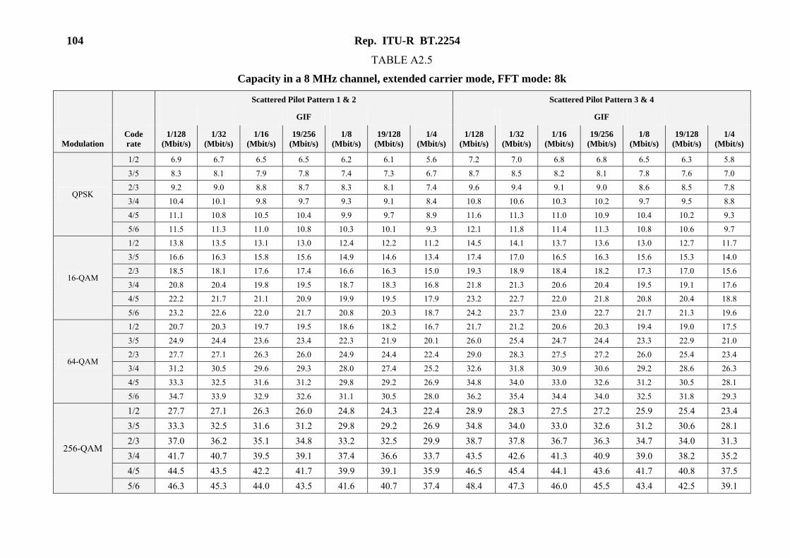
104 Rep. ITU-R BT.2254
TABLE A2.5
Capacity in a 8 MHz channel, extended carrier mode, FFT mode: 8k
Scattered Pilot Pattern 1 & 2 Scattered Pilot Pattern 3 & 4
GIF GIF
Modulation Code rate
1/128 (Mbit/s)
1/32 (Mbit/s)
1/16 (Mbit/s)
19/256 (Mbit/s)
1/8 (Mbit/s)
19/128 (Mbit/s)
1/4 (Mbit/s)
1/128 (Mbit/s)
1/32 (Mbit/s)
1/16 (Mbit/s)
19/256 (Mbit/s)
1/8 (Mbit/s)
19/128 (Mbit/s)
1/4 (Mbit/s)
QPSK
1/2 6.9 6.7 6.5 6.5 6.2 6.1 5.6 7.2 7.0 6.8 6.8 6.5 6.3 5.8
3/5 8.3 8.1 7.9 7.8 7.4 7.3 6.7 8.7 8.5 8.2 8.1 7.8 7.6 7.0
2/3 9.2 9.0 8.8 8.7 8.3 8.1 7.4 9.6 9.4 9.1 9.0 8.6 8.5 7.8
3/4 10.4 10.1 9.8 9.7 9.3 9.1 8.4 10.8 10.6 10.3 10.2 9.7 9.5 8.8
4/5 11.1 10.8 10.5 10.4 9.9 9.7 8.9 11.6 11.3 11.0 10.9 10.4 10.2 9.3
5/6 11.5 11.3 11.0 10.8 10.3 10.1 9.3 12.1 11.8 11.4 11.3 10.8 10.6 9.7
16-QAM
1/2 13.8 13.5 13.1 13.0 12.4 12.2 11.2 14.5 14.1 13.7 13.6 13.0 12.7 11.7
3/5 16.6 16.3 15.8 15.6 14.9 14.6 13.4 17.4 17.0 16.5 16.3 15.6 15.3 14.0
2/3 18.5 18.1 17.6 17.4 16.6 16.3 15.0 19.3 18.9 18.4 18.2 17.3 17.0 15.6
3/4 20.8 20.4 19.8 19.5 18.7 18.3 16.8 21.8 21.3 20.6 20.4 19.5 19.1 17.6
4/5 22.2 21.7 21.1 20.9 19.9 19.5 17.9 23.2 22.7 22.0 21.8 20.8 20.4 18.8
5/6 23.2 22.6 22.0 21.7 20.8 20.3 18.7 24.2 23.7 23.0 22.7 21.7 21.3 19.6
64-QAM
1/2 20.7 20.3 19.7 19.5 18.6 18.2 16.7 21.7 21.2 20.6 20.3 19.4 19.0 17.5
3/5 24.9 24.4 23.6 23.4 22.3 21.9 20.1 26.0 25.4 24.7 24.4 23.3 22.9 21.0
2/3 27.7 27.1 26.3 26.0 24.9 24.4 22.4 29.0 28.3 27.5 27.2 26.0 25.4 23.4
3/4 31.2 30.5 29.6 29.3 28.0 27.4 25.2 32.6 31.8 30.9 30.6 29.2 28.6 26.3
4/5 33.3 32.5 31.6 31.2 29.8 29.2 26.9 34.8 34.0 33.0 32.6 31.2 30.5 28.1
5/6 34.7 33.9 32.9 32.6 31.1 30.5 28.0 36.2 35.4 34.4 34.0 32.5 31.8 29.3
256-QAM
1/2 27.7 27.1 26.3 26.0 24.8 24.3 22.4 28.9 28.3 27.5 27.2 25.9 25.4 23.4
3/5 33.3 32.5 31.6 31.2 29.8 29.2 26.9 34.8 34.0 33.0 32.6 31.2 30.6 28.1
2/3 37.0 36.2 35.1 34.8 33.2 32.5 29.9 38.7 37.8 36.7 36.3 34.7 34.0 31.3
3/4 41.7 40.7 39.5 39.1 37.4 36.6 33.7 43.5 42.6 41.3 40.9 39.0 38.2 35.2
4/5 44.5 43.5 42.2 41.7 39.9 39.1 35.9 46.5 45.4 44.1 43.6 41.7 40.8 37.5
5/6 46.3 45.3 44.0 43.5 41.6 40.7 37.4 48.4 47.3 46.0 45.5 43.4 42.5 39.1
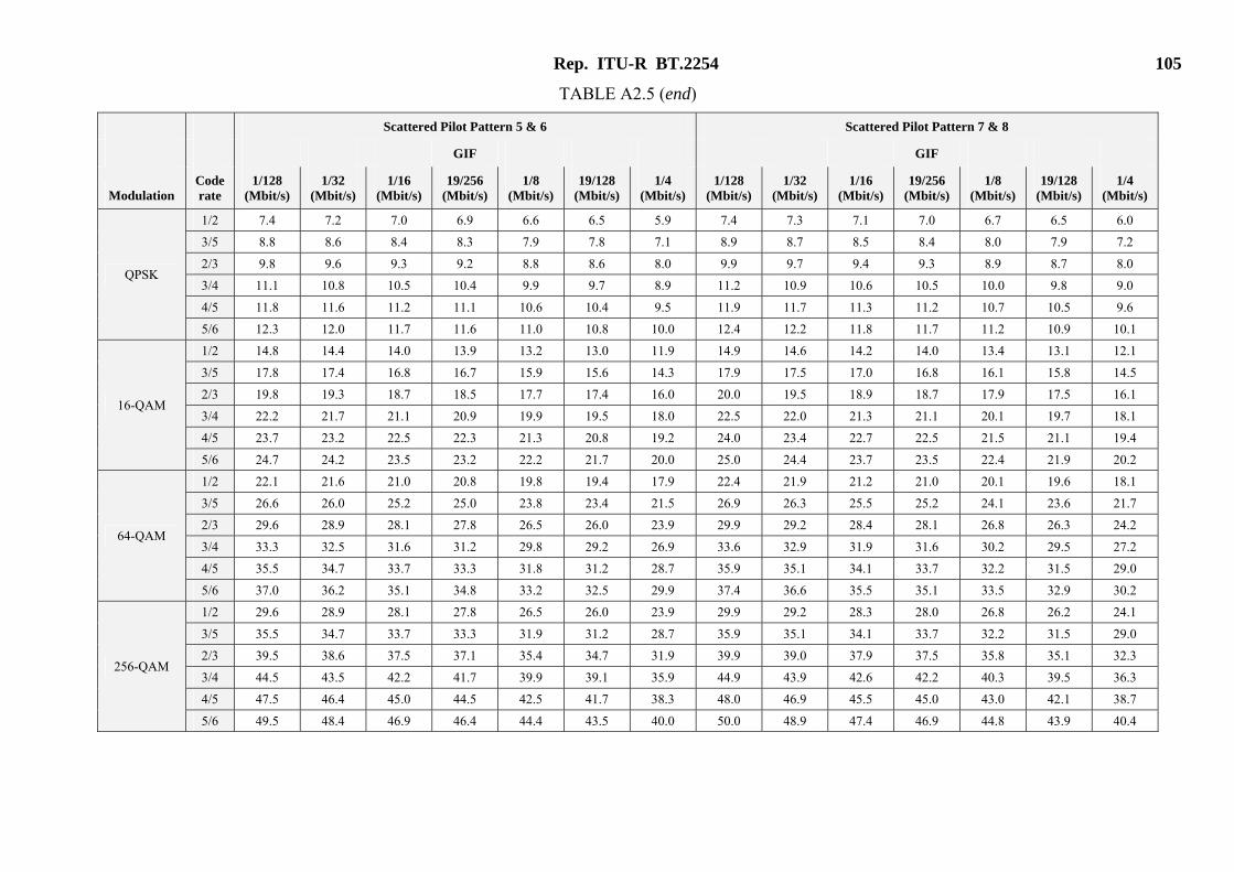
Rep. ITU-R BT.2254 105
TABLE A2.5 (end)
Scattered Pilot Pattern 5 & 6 Scattered Pilot Pattern 7 & 8
GIF GIF
Modulation Coderate
1/128 (Mbit/s)
1/32 (Mbit/s)
1/16 (Mbit/s)
19/256 (Mbit/s)
1/8 (Mbit/s)
19/128 (Mbit/s)
1/4 (Mbit/s)
1/128 (Mbit/s)
1/32 (Mbit/s)
1/16 (Mbit/s)
19/256 (Mbit/s)
1/8 (Mbit/s)
19/128 (Mbit/s)
1/4 (Mbit/s)
QPSK
1/2 7.4 7.2 7.0 6.9 6.6 6.5 5.9 7.4 7.3 7.1 7.0 6.7 6.5 6.0
3/5 8.8 8.6 8.4 8.3 7.9 7.8 7.1 8.9 8.7 8.5 8.4 8.0 7.9 7.2
2/3 9.8 9.6 9.3 9.2 8.8 8.6 8.0 9.9 9.7 9.4 9.3 8.9 8.7 8.0
3/4 11.1 10.8 10.5 10.4 9.9 9.7 8.9 11.2 10.9 10.6 10.5 10.0 9.8 9.0
4/5 11.8 11.6 11.2 11.1 10.6 10.4 9.5 11.9 11.7 11.3 11.2 10.7 10.5 9.6
5/6 12.3 12.0 11.7 11.6 11.0 10.8 10.0 12.4 12.2 11.8 11.7 11.2 10.9 10.1
16-QAM
1/2 14.8 14.4 14.0 13.9 13.2 13.0 11.9 14.9 14.6 14.2 14.0 13.4 13.1 12.1
3/5 17.8 17.4 16.8 16.7 15.9 15.6 14.3 17.9 17.5 17.0 16.8 16.1 15.8 14.5
2/3 19.8 19.3 18.7 18.5 17.7 17.4 16.0 20.0 19.5 18.9 18.7 17.9 17.5 16.1
3/4 22.2 21.7 21.1 20.9 19.9 19.5 18.0 22.5 22.0 21.3 21.1 20.1 19.7 18.1
4/5 23.7 23.2 22.5 22.3 21.3 20.8 19.2 24.0 23.4 22.7 22.5 21.5 21.1 19.4
5/6 24.7 24.2 23.5 23.2 22.2 21.7 20.0 25.0 24.4 23.7 23.5 22.4 21.9 20.2
64-QAM
1/2 22.1 21.6 21.0 20.8 19.8 19.4 17.9 22.4 21.9 21.2 21.0 20.1 19.6 18.1
3/5 26.6 26.0 25.2 25.0 23.8 23.4 21.5 26.9 26.3 25.5 25.2 24.1 23.6 21.7
2/3 29.6 28.9 28.1 27.8 26.5 26.0 23.9 29.9 29.2 28.4 28.1 26.8 26.3 24.2
3/4 33.3 32.5 31.6 31.2 29.8 29.2 26.9 33.6 32.9 31.9 31.6 30.2 29.5 27.2
4/5 35.5 34.7 33.7 33.3 31.8 31.2 28.7 35.9 35.1 34.1 33.7 32.2 31.5 29.0
5/6 37.0 36.2 35.1 34.8 33.2 32.5 29.9 37.4 36.6 35.5 35.1 33.5 32.9 30.2
256-QAM
1/2 29.6 28.9 28.1 27.8 26.5 26.0 23.9 29.9 29.2 28.3 28.0 26.8 26.2 24.1
3/5 35.5 34.7 33.7 33.3 31.9 31.2 28.7 35.9 35.1 34.1 33.7 32.2 31.5 29.0
2/3 39.5 38.6 37.5 37.1 35.4 34.7 31.9 39.9 39.0 37.9 37.5 35.8 35.1 32.3
3/4 44.5 43.5 42.2 41.7 39.9 39.1 35.9 44.9 43.9 42.6 42.2 40.3 39.5 36.3
4/5 47.5 46.4 45.0 44.5 42.5 41.7 38.3 48.0 46.9 45.5 45.0 43.0 42.1 38.7
5/6 49.5 48.4 46.9 46.4 44.4 43.5 40.0 50.0 48.9 47.4 46.9 44.8 43.9 40.4
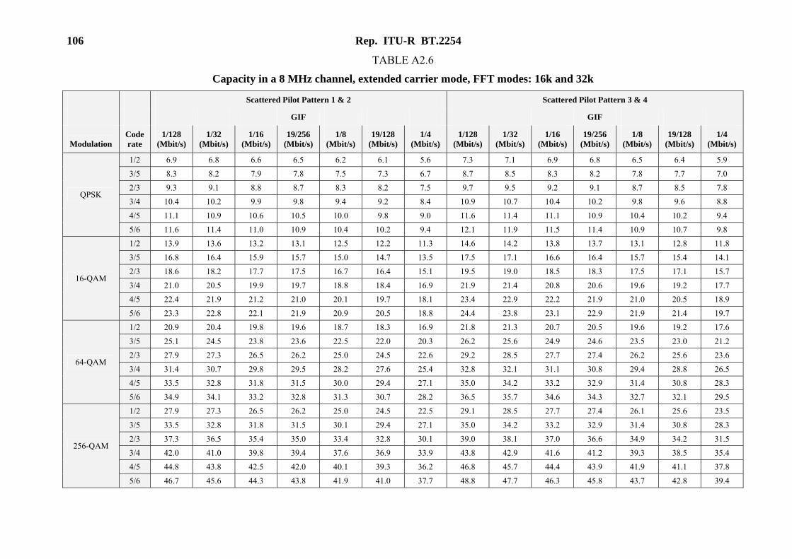
106 Rep. ITU-R BT.2254
TABLE A2.6
Capacity in a 8 MHz channel, extended carrier mode, FFT modes: 16k and 32k
Scattered Pilot Pattern 1 & 2 Scattered Pilot Pattern 3 & 4
GIF GIF
Modulation Coderate
1/128 (Mbit/s)
1/32 (Mbit/s)
1/16 (Mbit/s)
19/256 (Mbit/s)
1/8 (Mbit/s)
19/128 (Mbit/s)
1/4 (Mbit/s)
1/128 (Mbit/s)
1/32 (Mbit/s)
1/16 (Mbit/s)
19/256 (Mbit/s)
1/8 (Mbit/s)
19/128 (Mbit/s)
1/4 (Mbit/s)
QPSK
1/2 6.9 6.8 6.6 6.5 6.2 6.1 5.6 7.3 7.1 6.9 6.8 6.5 6.4 5.9
3/5 8.3 8.2 7.9 7.8 7.5 7.3 6.7 8.7 8.5 8.3 8.2 7.8 7.7 7.0
2/3 9.3 9.1 8.8 8.7 8.3 8.2 7.5 9.7 9.5 9.2 9.1 8.7 8.5 7.8
3/4 10.4 10.2 9.9 9.8 9.4 9.2 8.4 10.9 10.7 10.4 10.2 9.8 9.6 8.8
4/5 11.1 10.9 10.6 10.5 10.0 9.8 9.0 11.6 11.4 11.1 10.9 10.4 10.2 9.4
5/6 11.6 11.4 11.0 10.9 10.4 10.2 9.4 12.1 11.9 11.5 11.4 10.9 10.7 9.8
16-QAM
1/2 13.9 13.6 13.2 13.1 12.5 12.2 11.3 14.6 14.2 13.8 13.7 13.1 12.8 11.8
3/5 16.8 16.4 15.9 15.7 15.0 14.7 13.5 17.5 17.1 16.6 16.4 15.7 15.4 14.1
2/3 18.6 18.2 17.7 17.5 16.7 16.4 15.1 19.5 19.0 18.5 18.3 17.5 17.1 15.7
3/4 21.0 20.5 19.9 19.7 18.8 18.4 16.9 21.9 21.4 20.8 20.6 19.6 19.2 17.7
4/5 22.4 21.9 21.2 21.0 20.1 19.7 18.1 23.4 22.9 22.2 21.9 21.0 20.5 18.9
5/6 23.3 22.8 22.1 21.9 20.9 20.5 18.8 24.4 23.8 23.1 22.9 21.9 21.4 19.7
64-QAM
1/2 20.9 20.4 19.8 19.6 18.7 18.3 16.9 21.8 21.3 20.7 20.5 19.6 19.2 17.6
3/5 25.1 24.5 23.8 23.6 22.5 22.0 20.3 26.2 25.6 24.9 24.6 23.5 23.0 21.2
2/3 27.9 27.3 26.5 26.2 25.0 24.5 22.6 29.2 28.5 27.7 27.4 26.2 25.6 23.6
3/4 31.4 30.7 29.8 29.5 28.2 27.6 25.4 32.8 32.1 31.1 30.8 29.4 28.8 26.5
4/5 33.5 32.8 31.8 31.5 30.0 29.4 27.1 35.0 34.2 33.2 32.9 31.4 30.8 28.3
5/6 34.9 34.1 33.2 32.8 31.3 30.7 28.2 36.5 35.7 34.6 34.3 32.7 32.1 29.5
256-QAM
1/2 27.9 27.3 26.5 26.2 25.0 24.5 22.5 29.1 28.5 27.7 27.4 26.1 25.6 23.5
3/5 33.5 32.8 31.8 31.5 30.1 29.4 27.1 35.0 34.2 33.2 32.9 31.4 30.8 28.3
2/3 37.3 36.5 35.4 35.0 33.4 32.8 30.1 39.0 38.1 37.0 36.6 34.9 34.2 31.5
3/4 42.0 41.0 39.8 39.4 37.6 36.9 33.9 43.8 42.9 41.6 41.2 39.3 38.5 35.4
4/5 44.8 43.8 42.5 42.0 40.1 39.3 36.2 46.8 45.7 44.4 43.9 41.9 41.1 37.8
5/6 46.7 45.6 44.3 43.8 41.9 41.0 37.7 48.8 47.7 46.3 45.8 43.7 42.8 39.4
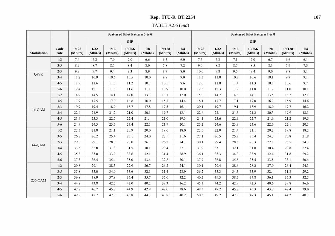
Rep. ITU-R BT.2254 107
TABLE A2.6 (end)
Scattered Pilot Pattern 5 & 6 Scattered Pilot Pattern 7 & 8
GIF GIF
Modulation Code rate
1/128 (Mbit/s)
1/32 (Mbit/s)
1/16 (Mbit/s)
19/256 (Mbit/s)
1/8 (Mbit/s)
19/128 (Mbit/s)
1/4 (Mbit/s)
1/128 (Mbit/s)
1/32 (Mbit/s)
1/16 (Mbit/s)
19/256 (Mbit/s)
1/8 (Mbit/s)
19/128 (Mbit/s)
1/4 (Mbit/s)
QPSK
1/2 7.4 7.2 7.0 7.0 6.6 6.5 6.0 7.5 7.3 7.1 7.0 6.7 6.6 6.1
3/5 8.9 8.7 8.5 8.4 8.0 7.8 7.2 9.0 8.8 8.5 8.5 8.1 7.9 7.3
2/3 9.9 9.7 9.4 9.3 8.9 8.7 8.0 10.0 9.8 9.5 9.4 9.0 8.8 8.1
3/4 11.2 10.9 10.6 10.5 10.0 9.8 9.0 11.3 11.0 10.7 10.6 10.1 9.9 9.1
4/5 11.9 11.6 11.3 11.2 10.7 10.5 9.6 12.0 11.8 11.4 11.3 10.8 10.6 9.7
5/6 12.4 12.1 11.8 11.6 11.1 10.9 10.0 12.5 12.3 11.9 11.8 11.2 11.0 10.1
16-QAM
1/2 14.9 14.5 14.1 14.0 13.3 13.1 12.0 15.0 14.7 14.3 14.1 13.5 13.2 12.1
3/5 17.9 17.5 17.0 16.8 16.0 15.7 14.4 18.1 17.7 17.1 17.0 16.2 15.9 14.6
2/3 19.9 19.4 18.9 18.7 17.8 17.5 16.1 20.1 19.7 19.1 18.9 18.0 17.7 16.2
3/4 22.4 21.9 21.2 21.0 20.1 19.7 18.1 22.6 22.1 21.5 21.2 20.3 19.9 18.3
4/5 23.9 23.3 22.7 22.4 21.4 21.0 19.3 24.1 23.6 22.9 22.7 21.6 21.2 19.5
5/6 24.9 24.3 23.6 23.4 22.3 21.9 20.1 25.2 24.6 23.9 23.6 22.6 22.1 20.3
64-QAM
1/2 22.3 21.8 21.1 20.9 20.0 19.6 18.0 22.5 22.0 21.4 21.1 20.2 19.8 18.2
3/5 26.8 26.2 25.4 25.1 24.0 23.5 21.6 27.1 26.5 25.7 25.4 24.3 23.8 21.9
2/3 29.8 29.1 28.3 28.0 26.7 26.2 24.1 30.1 29.4 28.6 28.3 27.0 26.5 24.3
3/4 33.5 32.8 31.8 31.5 30.1 29.4 27.1 33.9 33.1 32.1 31.8 30.4 29.8 27.4
4/5 35.8 35.0 33.9 33.6 32.1 31.4 28.9 36.1 35.3 34.3 33.9 32.4 31.8 29.2
5/6 37.3 36.4 35.4 35.0 33.4 32.8 30.1 37.7 36.8 35.8 35.4 33.8 33.1 30.4
256-QAM
1/2 29.8 29.1 28.3 27.9 26.7 26.2 24.1 30.1 29.4 28.6 28.2 27.0 26.4 24.3
3/5 35.8 35.0 34.0 33.6 32.1 31.4 28.9 36.2 35.3 34.3 33.9 32.4 31.8 29.2
2/3 39.8 38.9 37.8 37.4 35.7 35.0 32.2 40.2 39.3 38.2 37.8 36.1 35.3 32.5
3/4 44.8 43.8 42.5 42.0 40.2 39.3 36.2 45.3 44.2 42.9 42.5 40.6 39.8 36.6
4/5 47.8 46.7 45.3 44.9 42.9 42.0 38.6 48.3 47.2 45.8 45.3 43.3 42.4 39.0
5/6 49.8 48.7 47.3 46.8 44.7 43.8 40.2 50.3 49.2 47.8 47.3 45.1 44.2 40.7
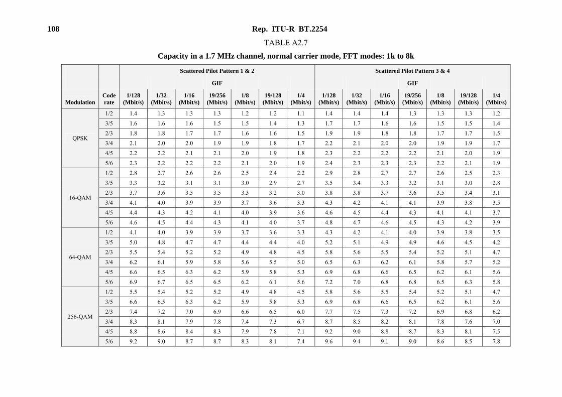
108 Rep. ITU-R BT.2254
TABLE A2.7
Capacity in a 1.7 MHz channel, normal carrier mode, FFT modes: 1k to 8k
Scattered Pilot Pattern 1 & 2 Scattered Pilot Pattern 3 & 4
GIF GIF
Modulation Coderate
1/128 (Mbit/s)
1/32 (Mbit/s)
1/16 (Mbit/s)
19/256(Mbit/s)
1/8 (Mbit/s)
19/128(Mbit/s)
1/4 (Mbit/s)
1/128 (Mbit/s)
1/32 (Mbit/s)
1/16 (Mbit/s)
19/256(Mbit/s)
1/8 (Mbit/s)
19/128(Mbit/s)
1/4 (Mbit/s)
QPSK
1/2 1.4 1.3 1.3 1.3 1.2 1.2 1.1 1.4 1.4 1.4 1.3 1.3 1.3 1.2
3/5 1.6 1.6 1.6 1.5 1.5 1.4 1.3 1.7 1.7 1.6 1.6 1.5 1.5 1.4
2/3 1.8 1.8 1.7 1.7 1.6 1.6 1.5 1.9 1.9 1.8 1.8 1.7 1.7 1.5
3/4 2.1 2.0 2.0 1.9 1.9 1.8 1.7 2.2 2.1 2.0 2.0 1.9 1.9 1.7
4/5 2.2 2.2 2.1 2.1 2.0 1.9 1.8 2.3 2.2 2.2 2.2 2.1 2.0 1.9
5/6 2.3 2.2 2.2 2.2 2.1 2.0 1.9 2.4 2.3 2.3 2.3 2.2 2.1 1.9
16-QAM
1/2 2.8 2.7 2.6 2.6 2.5 2.4 2.2 2.9 2.8 2.7 2.7 2.6 2.5 2.3
3/5 3.3 3.2 3.1 3.1 3.0 2.9 2.7 3.5 3.4 3.3 3.2 3.1 3.0 2.8
2/3 3.7 3.6 3.5 3.5 3.3 3.2 3.0 3.8 3.8 3.7 3.6 3.5 3.4 3.1
3/4 4.1 4.0 3.9 3.9 3.7 3.6 3.3 4.3 4.2 4.1 4.1 3.9 3.8 3.5
4/5 4.4 4.3 4.2 4.1 4.0 3.9 3.6 4.6 4.5 4.4 4.3 4.1 4.1 3.7
5/6 4.6 4.5 4.4 4.3 4.1 4.0 3.7 4.8 4.7 4.6 4.5 4.3 4.2 3.9
64-QAM
1/2 4.1 4.0 3.9 3.9 3.7 3.6 3.3 4.3 4.2 4.1 4.0 3.9 3.8 3.5
3/5 5.0 4.8 4.7 4.7 4.4 4.4 4.0 5.2 5.1 4.9 4.9 4.6 4.5 4.2
2/3 5.5 5.4 5.2 5.2 4.9 4.8 4.5 5.8 5.6 5.5 5.4 5.2 5.1 4.7
3/4 6.2 6.1 5.9 5.8 5.6 5.5 5.0 6.5 6.3 6.2 6.1 5.8 5.7 5.2
4/5 6.6 6.5 6.3 6.2 5.9 5.8 5.3 6.9 6.8 6.6 6.5 6.2 6.1 5.6
5/6 6.9 6.7 6.5 6.5 6.2 6.1 5.6 7.2 7.0 6.8 6.8 6.5 6.3 5.8
256-QAM
1/2 5.5 5.4 5.2 5.2 4.9 4.8 4.5 5.8 5.6 5.5 5.4 5.2 5.1 4.7
3/5 6.6 6.5 6.3 6.2 5.9 5.8 5.3 6.9 6.8 6.6 6.5 6.2 6.1 5.6
2/3 7.4 7.2 7.0 6.9 6.6 6.5 6.0 7.7 7.5 7.3 7.2 6.9 6.8 6.2
3/4 8.3 8.1 7.9 7.8 7.4 7.3 6.7 8.7 8.5 8.2 8.1 7.8 7.6 7.0
4/5 8.8 8.6 8.4 8.3 7.9 7.8 7.1 9.2 9.0 8.8 8.7 8.3 8.1 7.5
5/6 9.2 9.0 8.7 8.7 8.3 8.1 7.4 9.6 9.4 9.1 9.0 8.6 8.5 7.8
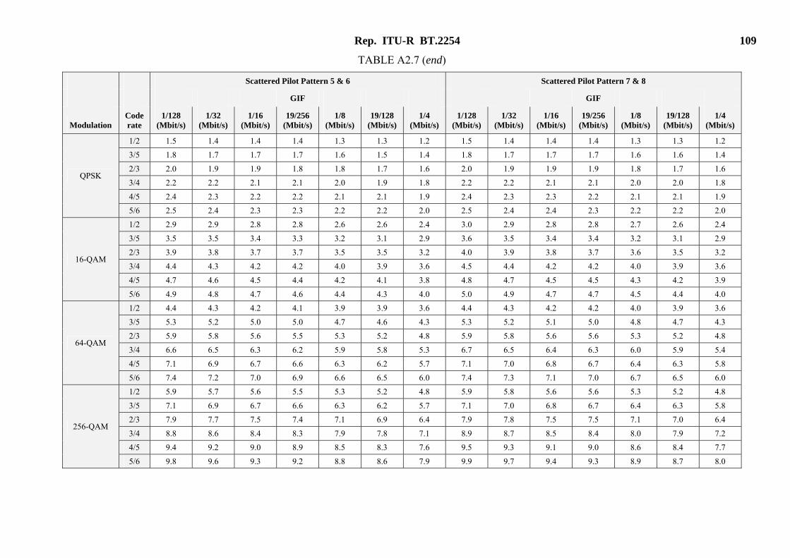
Rep. ITU-R BT.2254 109
TABLE A2.7 (end)
Scattered Pilot Pattern 5 & 6 Scattered Pilot Pattern 7 & 8
GIF GIF
Modulation Coderate
1/128 (Mbit/s)
1/32 (Mbit/s)
1/16 (Mbit/s)
19/256 (Mbit/s)
1/8 (Mbit/s)
19/128 (Mbit/s)
1/4 (Mbit/s)
1/128 (Mbit/s)
1/32 (Mbit/s)
1/16 (Mbit/s)
19/256 (Mbit/s)
1/8 (Mbit/s)
19/128 (Mbit/s)
1/4 (Mbit/s)
QPSK
1/2 1.5 1.4 1.4 1.4 1.3 1.3 1.2 1.5 1.4 1.4 1.4 1.3 1.3 1.2
3/5 1.8 1.7 1.7 1.7 1.6 1.5 1.4 1.8 1.7 1.7 1.7 1.6 1.6 1.4
2/3 2.0 1.9 1.9 1.8 1.8 1.7 1.6 2.0 1.9 1.9 1.9 1.8 1.7 1.6
3/4 2.2 2.2 2.1 2.1 2.0 1.9 1.8 2.2 2.2 2.1 2.1 2.0 2.0 1.8
4/5 2.4 2.3 2.2 2.2 2.1 2.1 1.9 2.4 2.3 2.3 2.2 2.1 2.1 1.9
5/6 2.5 2.4 2.3 2.3 2.2 2.2 2.0 2.5 2.4 2.4 2.3 2.2 2.2 2.0
16-QAM
1/2 2.9 2.9 2.8 2.8 2.6 2.6 2.4 3.0 2.9 2.8 2.8 2.7 2.6 2.4
3/5 3.5 3.5 3.4 3.3 3.2 3.1 2.9 3.6 3.5 3.4 3.4 3.2 3.1 2.9
2/3 3.9 3.8 3.7 3.7 3.5 3.5 3.2 4.0 3.9 3.8 3.7 3.6 3.5 3.2
3/4 4.4 4.3 4.2 4.2 4.0 3.9 3.6 4.5 4.4 4.2 4.2 4.0 3.9 3.6
4/5 4.7 4.6 4.5 4.4 4.2 4.1 3.8 4.8 4.7 4.5 4.5 4.3 4.2 3.9
5/6 4.9 4.8 4.7 4.6 4.4 4.3 4.0 5.0 4.9 4.7 4.7 4.5 4.4 4.0
64-QAM
1/2 4.4 4.3 4.2 4.1 3.9 3.9 3.6 4.4 4.3 4.2 4.2 4.0 3.9 3.6
3/5 5.3 5.2 5.0 5.0 4.7 4.6 4.3 5.3 5.2 5.1 5.0 4.8 4.7 4.3
2/3 5.9 5.8 5.6 5.5 5.3 5.2 4.8 5.9 5.8 5.6 5.6 5.3 5.2 4.8
3/4 6.6 6.5 6.3 6.2 5.9 5.8 5.3 6.7 6.5 6.4 6.3 6.0 5.9 5.4
4/5 7.1 6.9 6.7 6.6 6.3 6.2 5.7 7.1 7.0 6.8 6.7 6.4 6.3 5.8
5/6 7.4 7.2 7.0 6.9 6.6 6.5 6.0 7.4 7.3 7.1 7.0 6.7 6.5 6.0
256-QAM
1/2 5.9 5.7 5.6 5.5 5.3 5.2 4.8 5.9 5.8 5.6 5.6 5.3 5.2 4.8
3/5 7.1 6.9 6.7 6.6 6.3 6.2 5.7 7.1 7.0 6.8 6.7 6.4 6.3 5.8
2/3 7.9 7.7 7.5 7.4 7.1 6.9 6.4 7.9 7.8 7.5 7.5 7.1 7.0 6.4
3/4 8.8 8.6 8.4 8.3 7.9 7.8 7.1 8.9 8.7 8.5 8.4 8.0 7.9 7.2
4/5 9.4 9.2 9.0 8.9 8.5 8.3 7.6 9.5 9.3 9.1 9.0 8.6 8.4 7.7
5/6 9.8 9.6 9.3 9.2 8.8 8.6 7.9 9.9 9.7 9.4 9.3 8.9 8.7 8.0
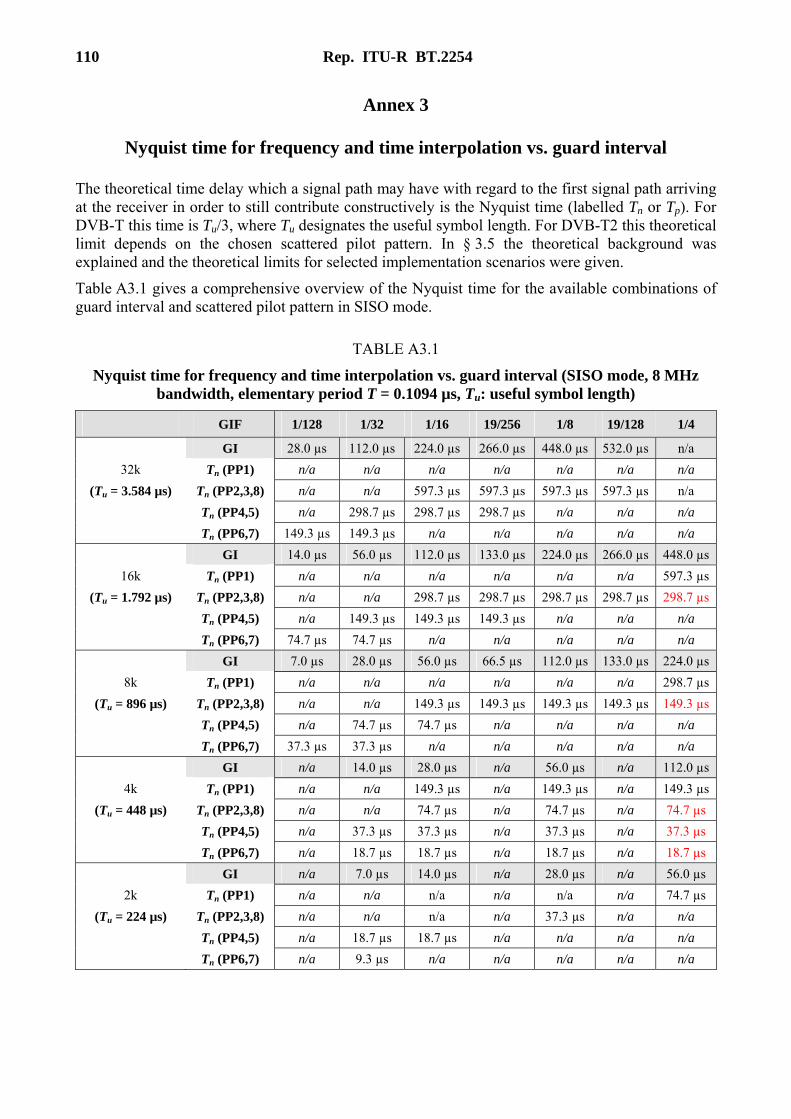
110 Rep. ITU-R BT.2254
Annex 3
Nyquist time for frequency and time interpolation vs. guard interval
The theoretical time delay which a signal path may have with regard to the first signal path arriving at the receiver in order to still contribute constructively is the Nyquist time (labelled Tn or Tp). For DVB-T this time is Tu/3, where Tu designates the useful symbol length. For DVB-T2 this theoretical limit depends on the chosen scattered pilot pattern. In § 3.5 the theoretical background was explained and the theoretical limits for selected implementation scenarios were given.
Table A3.1 gives a comprehensive overview of the Nyquist time for the available combinations of guard interval and scattered pilot pattern in SISO mode.
TABLE A3.1
Nyquist time for frequency and time interpolation vs. guard interval (SISO mode, 8 MHz bandwidth, elementary period T = 0.1094 µs, Tu: useful symbol length)
GIF 1/128 1/32 1/16 19/256 1/8 19/128 1/4
GI 28.0 µs 112.0 µs 224.0 µs 266.0 µs 448.0 µs 532.0 µs n/a
32k Tn (PP1) n/a n/a n/a n/a n/a n/a n/a
(Tu = 3.584 µs) Tn (PP2,3,8) n/a n/a 597.3 µs 597.3 µs 597.3 µs 597.3 µs n/a
Tn (PP4,5) n/a 298.7 µs 298.7 µs 298.7 µs n/a n/a n/a
Tn (PP6,7) 149.3 µs 149.3 µs n/a n/a n/a n/a n/a
GI 14.0 µs 56.0 µs 112.0 µs 133.0 µs 224.0 µs 266.0 µs 448.0 µs
16k Tn (PP1) n/a n/a n/a n/a n/a n/a 597.3 µs
(Tu = 1.792 µs) Tn (PP2,3,8) n/a n/a 298.7 µs 298.7 µs 298.7 µs 298.7 µs 298.7 µs
Tn (PP4,5) n/a 149.3 µs 149.3 µs 149.3 µs n/a n/a n/a
Tn (PP6,7) 74.7 µs 74.7 µs n/a n/a n/a n/a n/a
GI 7.0 µs 28.0 µs 56.0 µs 66.5 µs 112.0 µs 133.0 µs 224.0 µs
8k Tn (PP1) n/a n/a n/a n/a n/a n/a 298.7 µs
(Tu = 896 µs) Tn (PP2,3,8) n/a n/a 149.3 µs 149.3 µs 149.3 µs 149.3 µs 149.3 µs
Tn (PP4,5) n/a 74.7 µs 74.7 µs n/a n/a n/a n/a
Tn (PP6,7) 37.3 µs 37.3 µs n/a n/a n/a n/a n/a
GI n/a 14.0 µs 28.0 µs n/a 56.0 µs n/a 112.0 µs
4k Tn (PP1) n/a n/a 149.3 µs n/a 149.3 µs n/a 149.3 µs
(Tu = 448 µs) Tn (PP2,3,8) n/a n/a 74.7 µs n/a 74.7 µs n/a 74.7 µs
Tn (PP4,5) n/a 37.3 µs 37.3 µs n/a 37.3 µs n/a 37.3 µs
Tn (PP6,7) n/a 18.7 µs 18.7 µs n/a 18.7 µs n/a 18.7 µs
GI n/a 7.0 µs 14.0 µs n/a 28.0 µs n/a 56.0 µs
2k Tn (PP1) n/a n/a n/a n/a n/a n/a 74.7 µs
(Tu = 224 µs) Tn (PP2,3,8) n/a n/a n/a n/a 37.3 µs n/a n/a
Tn (PP4,5) n/a 18.7 µs 18.7 µs n/a n/a n/a n/a
Tn (PP6,7) n/a 9.3 µs n/a n/a n/a n/a n/a
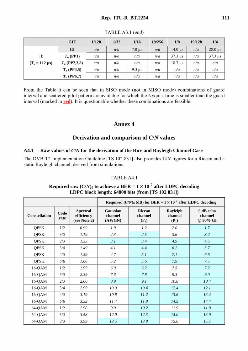
Rep. ITU-R BT.2254 111
TABLE A3.1 (end)
GIF 1/128 1/32 1/16 19/256 1/8 19/128 1/4
GI n/a n/a 7.0 µs n/a 14.0 µs n/a 28.0 µs
1k Tn (PP1) n/a n/a n/a n/a 37.3 µs n/a 37.3 µs
(Tu = 112 µs) Tn (PP2,3,8) n/a n/a n/a n/a 18.7 µs n/a n/a
Tn (PP4,5) n/a n/a 9.3 µs n/a n/a n/a n/a
Tn (PP6,7) n/a n/a n/a n/a n/a n/a n/a
From the Table it can be seen that in SISO mode (not in MISO mode) combinations of guard interval and scattered pilot pattern are available for which the Nyquist time is smaller than the guard interval (marked in red). It is questionable whether these combinations are feasible.
Annex 4
Derivation and comparison of C/N values
A4.1 Raw values of C/N for the derivation of the Rice and Rayleigh Channel Case
The DVB-T2 Implementation Guideline [TS 102 831] also provides C/N figures for a Ricean and a static Rayleigh channel, derived from simulations.
TABLE A4.1
Required raw (C/N)0 to achieve a BER = 1 × 10⁻⁷ after LDPC decoding LDPC block length: 64800 bits (from [TS 102 831])
Required (C/N)0 (dB) for BER = 1 × 10⁻⁷ after LDPC decoding
Constellation Code rate
Spectral efficiency
(see Note 2)
Gaussian channel
(AWGN)
Ricean channel
(F1)
Rayleigh channel
(P1)
0 dB echo channel
@ 90% GI
QPSK 1/2 0.99 1.0 1.2 2.0 1.7
QPSK 3/5 1.19 2.3 2.5 3.6 3.2
QPSK 2/3 1.33 3.1 3.4 4.9 4.5
QPSK 3/4 1.49 4.1 4.4 6.2 5.7
QPSK 4/5 1.59 4.7 5.1 7.1 6.6
QPSK 5/6 1.66 5.2 5.6 7.9 7.5
16-QAM 1/2 1.99 6.0 6.2 7.5 7.2
16-QAM 3/5 2.39 7.6 7.8 9.3 9.0
16-QAM 2/3 2.66 8.9 9.1 10.8 10.4
16-QAM 3/4 2.99 10.0 10.4 12.4 12.1
16-QAM 4/5 3.19 10.8 11.2 13.6 13.4
16-QAM 5/6 3.32 11.4 11.8 14.5 14.4
64-QAM 1/2 2.98 9.9 10.2 11.9 11.8
64-QAM 3/5 3.58 12.0 12.3 14.0 13.9
64-QAM 2/3 3.99 13.5 13.8 15.6 15.5
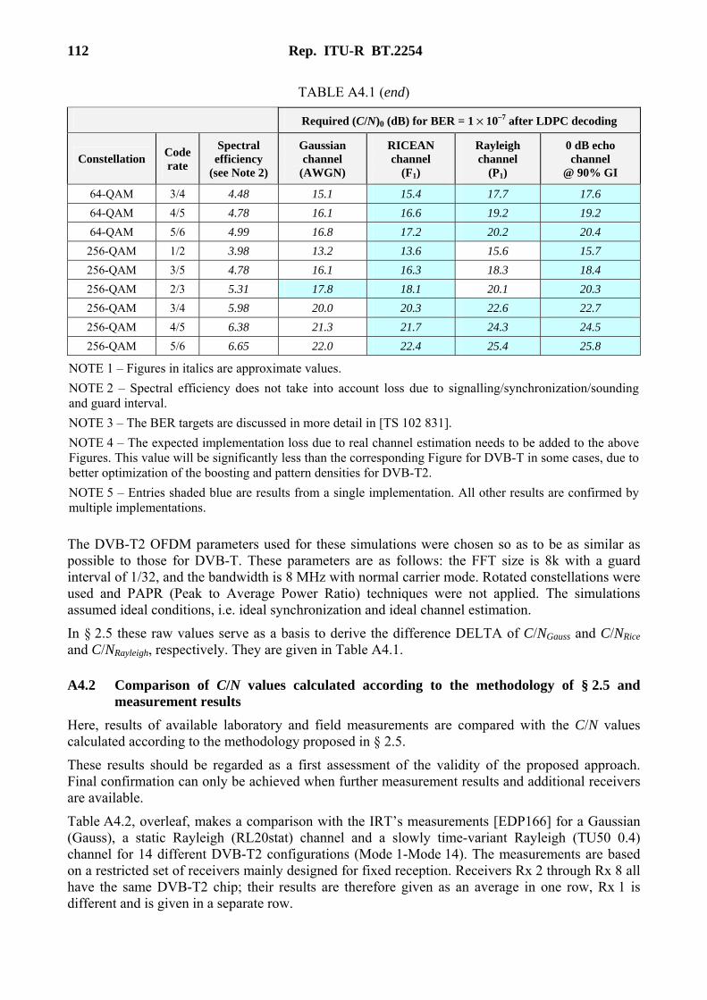
112 Rep. ITU-R BT.2254
TABLE A4.1 (end)
Required (C/N)0 (dB) for BER = 1 × 10⁻⁷ after LDPC decoding
Constellation Code rate
Spectral efficiency
(see Note 2)
Gaussian channel
(AWGN)
RICEAN channel
(F1)
Rayleigh channel
(P1)
0 dB echo channel
@ 90% GI
64-QAM 3/4 4.48 15.1 15.4 17.7 17.6
64-QAM 4/5 4.78 16.1 16.6 19.2 19.2
64-QAM 5/6 4.99 16.8 17.2 20.2 20.4
256-QAM 1/2 3.98 13.2 13.6 15.6 15.7
256-QAM 3/5 4.78 16.1 16.3 18.3 18.4
256-QAM 2/3 5.31 17.8 18.1 20.1 20.3
256-QAM 3/4 5.98 20.0 20.3 22.6 22.7
256-QAM 4/5 6.38 21.3 21.7 24.3 24.5
256-QAM 5/6 6.65 22.0 22.4 25.4 25.8
NOTE 1 – Figures in italics are approximate values.
NOTE 2 – Spectral efficiency does not take into account loss due to signalling/synchronization/sounding and guard interval.
NOTE 3 – The BER targets are discussed in more detail in [TS 102 831].
NOTE 4 – The expected implementation loss due to real channel estimation needs to be added to the above Figures. This value will be significantly less than the corresponding Figure for DVB-T in some cases, due to better optimization of the boosting and pattern densities for DVB-T2.
NOTE 5 – Entries shaded blue are results from a single implementation. All other results are confirmed by multiple implementations.
The DVB-T2 OFDM parameters used for these simulations were chosen so as to be as similar as possible to those for DVB-T. These parameters are as follows: the FFT size is 8k with a guard interval of 1/32, and the bandwidth is 8 MHz with normal carrier mode. Rotated constellations were used and PAPR (Peak to Average Power Ratio) techniques were not applied. The simulations assumed ideal conditions, i.e. ideal synchronization and ideal channel estimation.
In § 2.5 these raw values serve as a basis to derive the difference DELTA of C/NGauss and C/NRice and C/NRayleigh, respectively. They are given in Table A4.1.
A4.2 Comparison of C/N values calculated according to the methodology of § 2.5 and measurement results
Here, results of available laboratory and field measurements are compared with the C/N values calculated according to the methodology proposed in § 2.5.
These results should be regarded as a first assessment of the validity of the proposed approach. Final confirmation can only be achieved when further measurement results and additional receivers are available.
Table A4.2, overleaf, makes a comparison with the IRT’s measurements [EDP166] for a Gaussian (Gauss), a static Rayleigh (RL20stat) channel and a slowly time-variant Rayleigh (TU50 0.4) channel for 14 different DVB-T2 configurations (Mode 1-Mode 14). The measurements are based on a restricted set of receivers mainly designed for fixed reception. Receivers Rx 2 through Rx 8 all have the same DVB-T2 chip; their results are therefore given as an average in one row, Rx 1 is different and is given in a separate row.

Rep. ITU-R BT.2254 113
One can see that the figures show agreement within 1-3 dB, which is not too bad since the measurement results themselves show differences of 2 dB or even more.
The calculated values are higher by 2-3 dB for the Gaussian channel. For the Rayleigh channel case the calculated values are 1-2 dB higher than the measured values for the static Rayleigh case, but fit quite well within 1 dB for the time-variant Rayleigh case.
In general, the calculated C/N values can be regarded as conservative compared to the measurement results for the Gaussian channel. They fit quite well for the Rayleigh channel case.
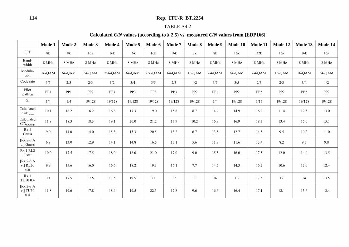
114 Rep. ITU-R BT.2254
TABLE A4.2
Calculated C/N values (according to § 2.5) vs. measured C/N values from [EDP166]
Mode 1 Mode 2 Mode 3 Mode 4 Mode 5 Mode 6 Mode 7 Mode 8 Mode 9 Mode 10 Mode 11 Mode 12 Mode 13 Mode 14
FFT 8k 8k 16k 16k 16k 16k 16k 8k 8k 16k 32k 16k 16k 16k
Band-width
8 MHz 8 MHz 8 MHz 8 MHz 8 MHz 8 MHz 8 MHz 8 MHz 8 MHz 8 MHz 8 MHz 8 MHz 8 MHz 8 MHz
Modula-tion
16-QAM 64-QAM 64-QAM 256-QAM 64-QAM 256-QAM 64-QAM 16-QAM 64-QAM 64-QAM 64-QAM 16-QAM 16-QAM 64-QAM
Code rate 3/5 2/3 2/3 1/2 3/4 3/5 2/3 1/2 3/5 3/5 2/3 2/3 3/4 1/2
Pilot pattern
PP1 PP1 PP2 PP3 PP3 PP3 PP3 PP2 PP1 PP2 PP2 PP2 PP2 PP2
GI 1/4 1/4 19/128 19/128 19/128 19/128 19/128 19/128 1/4 19/128 1/16 19/128 19/128 19/128
Calculated C/NGauss
10.1 16.2 16.2 16.6 17.3 19.0 15.8 8.7 14.9 14.9 16.2 11.4 12.5 13.0
Calculated C/NRayleigh
11.8 18.3 18.3 19.1 20.0 21.2 17.9 10.2 16.9 16.9 18.3 13.4 15.0 15.1
Rx 1 Gauss
9.0 14.0 14.0 15.3 15.3 20.5 13.2 6.7 13.5 12.7 14.5 9.5 10.2 11.0
[Rx 2-8 Av.] Gauss
6.9 13.0 12.9 14.1 14.8 16.5 13.1 5.6 11.8 11.6 13.4 8.2 9.3 9.8
Rx 1 RL20 stat
10.0 17.5 17.5 18.0 18.0 21.0 17.0 9.0 15.5 16.0 17.5 12.0 14.0 13.5
[Rx 2-8 Av.] RL20
stat 9.9 15.6 16.0 16.6 18.2 19.3 16.1 7.7 14.5 14.3 16.2 10.6 12.0 12.4
Rx 1 TU50 0.4
13 17.5 17.5 17.5 19.5 21 17 9 16 16 17.5 12 14 13.5
[Rx 2-8 Av.] TU50
0.4 11.8 19.6 17.8 18.4 19.5 22.3 17.8 9.6 16.6 16.4 17.1 12.1 13.6 13.4

Rep. ITU-R BT.2254 115
A second comparison uses results of measurements [EDP135, Ei2010, Ei2011] of the University of the Basque Country. These are field and laboratory measurements for fixed reception. Channel classification is made based on the standard deviation of spectral amplitudes of the received signal according to Recommendation ITU-R SM.1875 [SM1875].
The measurements are taken with the following receivers:
Table A4.3: Two consumer receivers.
Table A4.4: Professional receiver (Enensys)
Table A4.5: Software receiver.
The Nordig Requirements for receivers [NorDig2010] are also included in Table A4.4 for the available channels.
It must be noted that the channel models are not the same:
– Nordig 0 dB echo channel does not include frequency offset between paths.
– In laboratory tests, Ricean and Rayleigh channels are obtained by two paths of different attenuation and a delay of 50% of the GI.
– In field trials, multipath is in some cases produced by SFN configurations, with one main transmitter and a gap-filler, and in other cases only by the propagation channel.
All the measured configurations employ 64- or 256-QAM modulations, pilot patterns PP7 with 1/128 GIF or PP4 with 1/16 GIF, 8 MHz bandwidth with extended mode and rotated constellations.
TABLE A4.3
Comparison of calculated C/N values (according to § 2.5) and measured C/N values from [EDP135]
32k FFT, 8 MHz Extended mode, Pilot Pattern PP4, Ricean channel
Modulation Code Rate Measured C/N (dB) Calculated C/NRice (dB)
64-QAM 1/2 11.9 12.9
64-QAM 3/5 13.4 14.8
64-QAM 2/3 14.9 16.1
64-QAM 3/4 16.2 17.6
64-QAM 4/5 17.5 18.9
64-QAM 5/6 18.1 19.4
256-QAM 1/2 16.1 17.0
256-QAM 3/5 18.3 19.2
256-QAM 2/3 19.7 20.8
256-QAM 3/4 22.0 22.8
256-QAM 4/5 23.2 24.4
256-QAM 5/6 24.2 25.2
The calculated C/N values are slightly higher than the measured values by about 1 dB.

116 Rep. ITU-R BT.2254
TABLE A4.4
Comparison of calculated C/N values (according to § 2.5), NorDig values, and measured C/N values from lab tests and field trials from [Ei2011]
32k FFT, 8 MHz Extended mode, Pilot pattern PP4, GIF 1/16
QAM 64 64 64 64 64 64 256 256 256 256 256 256
Code Rate 1/2 3/5 2/3 3/4 4/5 5/6 1/2 3/5 2/3 3/4 4/5 5/6
Gauss.
Simulation 9.9 12.0 13.5 15.1 16.1 16.8 13.2 16.1 17.8 20.0 21.3 22.0
NorDig 12.6 14.4 15.7 17.3 18.3 18.9 16.5 18.9 20.4 22.4 23.8 24.6
Lab 10.9 12.8 14.0 15.6 16.6 17.3 15.0 17.4 18.7 20.8 22.3 23.1
Field 11.2 13.0 14.3 15.9 17.0 17.6 15.3 17.8 19.2 21.4 22.8 23.7
Calculated 12.6 14.5 15.8 17.3 18.3 19.0 16.6 19.0 20.4 22.4 23.9 24.7
Rice
Simulation 10.2 12.3 13.8 15.4 16.6 17.2 13.6 16.3 18.1 20.3 21.7 22.4
Lab 11.3 13.1 14.4 16.0 17.1 17.8 15.3 17.7 19.1 21.4 22.7 25.8
Field 11.4 13.4 14.7 16.6 17.6 18.3 15.8 18.4 19.8 22.3 24.2 24.8
Calculated 12.9 14.8 16.1 17.6 18.9 19.4 17.0 19.2 20.8 22.8 24.4 25.2
Rayleigh
Simulation 11.9 14.0 15.6 17.7 19.2 20.2 15.6 18.3 20.1 22.6 24.3 25.4
Lab 12.9 14.9 16.5 18.5 20.0 21.0 17.0 19.5 21.3 23.8 25.8 26.2
Field 13.4 15.6 17.4 19.6 21.4 22.1 17.9 20.7 22.7 25.9 28.5 28.9
Calculated 14.7 16.5 17.9 20.0 21.6 22.6 19.1 21.3 22.9 25.4 27.5 28.9
0 dB eco
Simulation 11.8 13.9 15.5 17.6 19.2 20.4 15.7 18.4 20.3 22.7 24.5 25.8
Nordig 15.5 17.6 19.2 21.6 23.5 25.0 20.2 22.6 24.6 27.4 30.2 32.7
Lab 13.7 15.9 17.9 20.5 22.6 24.2 18.1 20.8 22.7 25.7 28.6 32.1
32k FFT, 8 MHz Extended mode, Pilot pattern PP7, GIF 1/128
QAM
256 256 256 256 256 256
Code Rate 1/2 3/5 2/3 3/4 4/5 5/6
Gauss.
Simulation 13.2 16.1 17.8 20.0 21.3 22.0
Nordig 15.9 18.3 19.7 21.7 23.2 23.9
Lab 15.0 17.4 18.9 20.8 22.4 23.1
Field 15.2 17.7 19.0 21.3 22.8 23.7
Calculated 15.9 18.2 19.7 21.7 23.1 23.9
Rice
Simulation 13.6 16.3 18.1 20.3 21.7 22.4
Lab 15.5 17.8 19.1 21.3 22.6 23.5
Field 15.6 18.2 19.7 22.2 23.6 24.8
Calculated 16.3 18.4 20.0 22.0 23.6 24.4
Rayleigh
Simulation 15.6 18.3 20.1 22.6 24.3 25.4
Lab 17.0 19.6 21.4 23.8 25.8 27.4
Field 17.8 20.9 22.2 27.1 28.1 32.6
Calculated 18.3 20.5 22.1 24.6 26.6 28.0
0 dB eco
Simulation 15.7 18.4 20.3 22.7 24.5 25.8
Nordig 19.5 22.0 23.9 26.6 29.3 31.6
Lab 18.9 21.7 23.2 26.1 29.2 31.9

Rep. ITU-R BT.2254 117
As indicated in § 2.5, the calculated C/N are identical to the NorDig figures for the Gaussian channel within 0.1 dB.
For the Gaussian channel, the calculated C/N are about 1 to 2 dB higher than the measured values from laboratory and field trials. For the Ricean channel the calculated C/N are higher by 0-1 dB than the measured figures, and for the Rayleigh channel the calculated C/N fit quite good with the measured C/N. In the case of DVB-T2 mode 256-QAM, PP7, for the Rayleigh channel, even higher values have been measured than calculated by the methodology of § 2.5.
These results are in line with the findings of the IRT measurements which indicate that the calculated C/N figures are slightly conservative with regard to the Gaussian channel. They fit reasonably well in the Rice and the Rayleigh case.
TABLE A4.5
Comparison of calculated C/N values (according to § 2.5) and measured C/N values from [Ei2010]
32k FFT, 8 MHz Extended mode, Pilot pattern PP7, Ricean channel
Modulation Code Rate Measured C/N (dB) Calculated C/NRice (dB)
64-QAM 3/4 16.0 16.9
256-QAM 3/5 18.0 18.4
Again, the calculated values are 0.5-1 dB higher than the measured values.
The overall calculated C/N figures are slightly conservative for many T2 modes particularly for the Gaussian channel. It has to be kept in mind that the measurement results are yet based on a relatively small number of receivers.
118 Rep. ITU-R BT.2254
Annex 5
DVB-T2-Lite
A5.1 Introduction
DVB-T2-Lite is a system profile which was added in version 1.3.1 of the DVB-T2 specification in November 2011 [EN 302 755-V1.3.1]. It is particularly designed for mobile and handheld reception. With T2-Lite the set of possible system configurations is restricted as compared to the full range of options provided by DVB-T2 as described in version 1.2.1 of the system specification. In order to distinguish T2-Lite from this full range of options the latter is called T2-Base. However, T2-Lite also adds some new options that are not available in T2-Base. Thus T2-Base does not describe the full superset of DVB-T2 options that now exist.
In general, T2-Lite reduces the complexity that is required for the reception of only T2-Lite services, serving to reduce the cost and power consumption for receivers designed for handheld and mobile reception.
In § A5.2 the differences between T2-Base and T2-Lite are listed as far as they are relevant for frequency and network planning. Section A5.3 describes how the T2-Lite data stream can be integrated in the DVB-T2 multiplex. Sections A5.4 and A5.5 give details of system and planning parameters, although for C/N and protection ratios only limited information is currently publicly available. Section A5.6 discusses some possible implementation scenarios and practical implementation aspects.
An update of the DVB-T2 implementation guideline including DVB-T2-Lite aspects will soon be made available by ETSI.
A5.2 Differences between T2-Base and T2-Lite
Differences between DVB-T2-Lite and DVB-T2-Base relevant for planning are:
– Additional, more robust code rates 1/3 and 2/5 are available
– Sensitive code rates 4/5 and 5/6 are omitted
– 256-QAM modulation is possible, but not with code rates 2/3 and 3/4, and no rotated constellation is possible with 256-QAM
– The maximum data rate is restricted to 4 Mbit/s
– FFT sizes 1k and 32k are omitted
– Pilot pattern PP8 is not possible
– Long FEC (64k) is omitted
– Only a reduced time interleaving memory is available
– The number of combinations of FFT size, GI and PP is restricted
– Additional optional error protection is available (scrambling of L1 post-signalling)
– Longer FEF blocks are possible (up to 1000 ms).
A5.3 DVB-T2-Lite signal structure
In principle, a combination of T2-Lite and T2-Base services is achieved by means of the future extension frame (FEF) or the physical layer pipe (PLP) mechanism. The T2-Lite profile is signalled to the receiver via the L1-signalling.
There are several possibilities for a T2-Lite transmission.
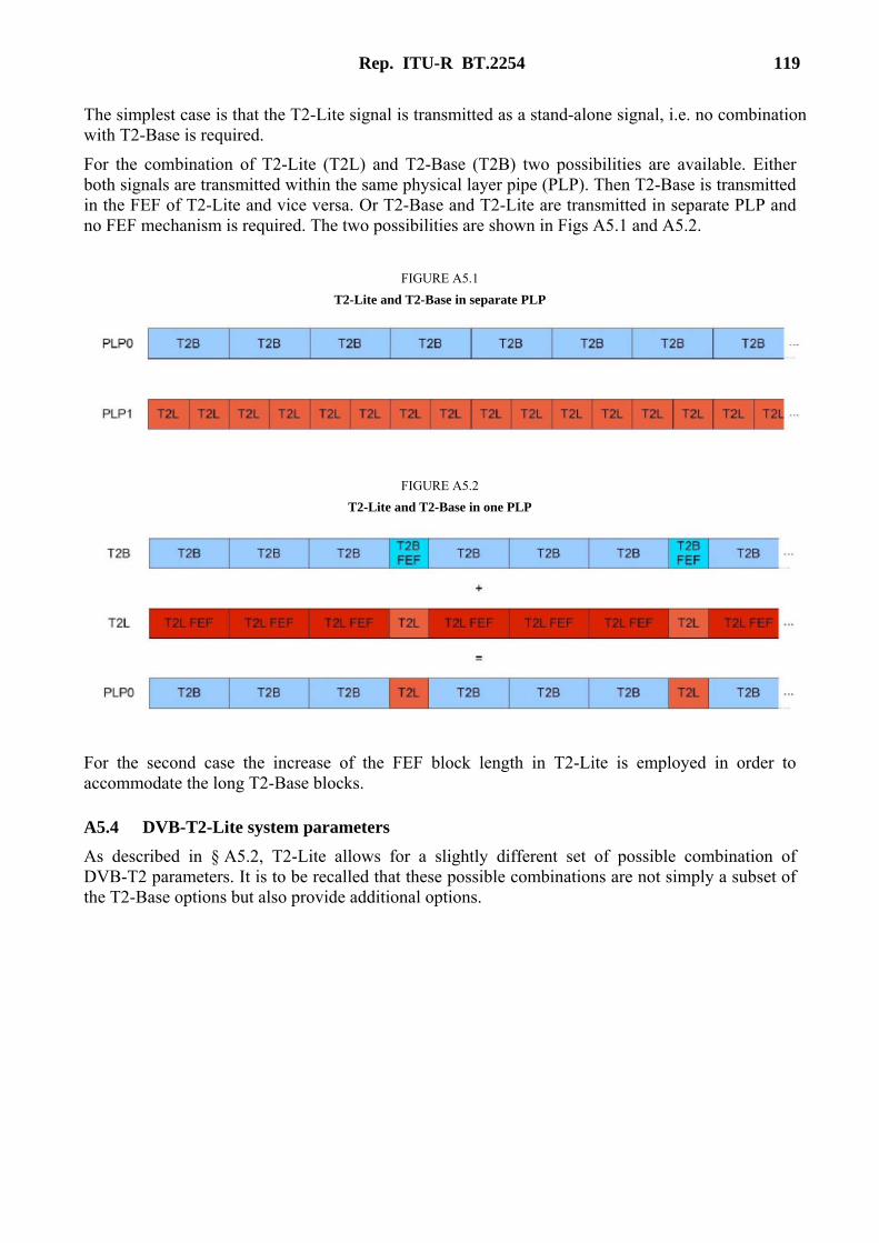
Rep. ITU-R BT.2254 119
The simplest case is that the T2-Lite signal is transmitted as a stand-alone signal, i.e. no combination with T2-Base is required.
For the combination of T2-Lite (T2L) and T2-Base (T2B) two possibilities are available. Either both signals are transmitted within the same physical layer pipe (PLP). Then T2-Base is transmitted in the FEF of T2-Lite and vice versa. Or T2-Base and T2-Lite are transmitted in separate PLP and no FEF mechanism is required. The two possibilities are shown in Figs A5.1 and A5.2.
FIGURE A5.1
T2-Lite and T2-Base in separate PLP
FIGURE A5.2
T2-Lite and T2-Base in one PLP
For the second case the increase of the FEF block length in T2-Lite is employed in order to accommodate the long T2-Base blocks.
A5.4 DVB-T2-Lite system parameters
As described in § A5.2, T2-Lite allows for a slightly different set of possible combination of DVB-T2 parameters. It is to be recalled that these possible combinations are not simply a subset of the T2-Base options but also provide additional options.
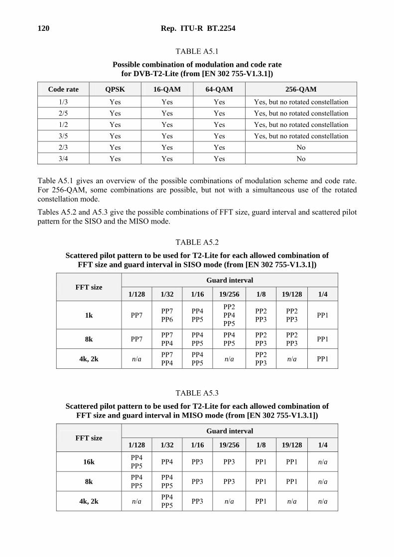
120 Rep. ITU-R BT.2254
TABLE A5.1
Possible combination of modulation and code rate for DVB-T2-Lite (from [EN 302 755-V1.3.1])
Code rate QPSK 16-QAM 64-QAM 256-QAM
1/3 Yes Yes Yes Yes, but no rotated constellation
2/5 Yes Yes Yes Yes, but no rotated constellation
1/2 Yes Yes Yes Yes, but no rotated constellation
3/5 Yes Yes Yes Yes, but no rotated constellation
2/3 Yes Yes Yes No
3/4 Yes Yes Yes No
Table A5.1 gives an overview of the possible combinations of modulation scheme and code rate. For 256-QAM, some combinations are possible, but not with a simultaneous use of the rotated constellation mode.
Tables A5.2 and A5.3 give the possible combinations of FFT size, guard interval and scattered pilot pattern for the SISO and the MISO mode.
TABLE A5.2
Scattered pilot pattern to be used for T2-Lite for each allowed combination of FFT size and guard interval in SISO mode (from [EN 302 755-V1.3.1])
FFT size Guard interval
1/128 1/32 1/16 19/256 1/8 19/128 1/4
1k PP7 PP7 PP6
PP4 PP5
PP2 PP4 PP5
PP2 PP3
PP2 PP3
PP1
8k PP7 PP7 PP4
PP4 PP5
PP4 PP5
PP2 PP3
PP2 PP3
PP1
4k, 2k n/a PP7 PP4
PP4 PP5
n/a PP2 PP3
n/a PP1
TABLE A5.3
Scattered pilot pattern to be used for T2-Lite for each allowed combination of FFT size and guard interval in MISO mode (from [EN 302 755-V1.3.1])
FFT size Guard interval
1/128 1/32 1/16 19/256 1/8 19/128 1/4
16k PP4 PP5
PP4 PP3 PP3 PP1 PP1 n/a
8k PP4 PP5
PP4 PP5
PP3 PP3 PP1 PP1 n/a
4k, 2k n/a PP4 PP5
PP3 n/a PP1 n/a n/a

Rep. ITU-R BT.2254 121
A5.5 DVB-T2-Lite planning parameters
It is assumed that a T2-Lite mode shows the same sensitivity as the corresponding T2-Base mode. This implies that C/N values and protection ratios as described in § 2.5 and § 3.4 may be used for frequency and network planning.
To date no simulation or measurement results are publicly available for the additional code rates 1/3 and 2/5. However, these code rates are also available in DVB-S2.
Simulation results for DVB-S2 in a Gaussian channel [EN 302 307] are given in Table A5.4 and are compared with raw C/N for DVB-T2 from Table 2.9.
For the higher code rates the C/N figures are identical. Therefore, it can be expected that for the lower code rates in T2-Lite the figures in Table A5.4 apply. Corresponding C/N values for planning may then be derived as described in § 2.5.
TABLE A5.4
Raw C/N for DVB-T2 and DVB-S2 for QPSK modes (from [EN 302 755-V1.3.1] and [EN 302 307])
Mode Raw C/N (dB) DVB-T2 Raw C/N (dB) DVB-S2
QPSK 1/4 n/a –2.4
QPSK 1/3 n/a –1.2
QPSK 2/5 n/a –0.3
QPSK 1/2 1.0 1.0
QPSK 3/5 2.2 2.2
QPSK 2/3 3.1 3.1
QPSK 3/4 4.1 4.0
QPSK 4/5 4.7 4.7
QPSK 5/6 5.2 5.2
QPSK 8/9 n/a 6.2
QPSK 9/10 n/a 6.4
More information will be covered in an update of this Report when it becomes available.
A5.6 Implementation aspects and implementation scenarios
T2-Lite has the same SFN capability as the T2-Base.
To update a T2-Base transmitter to a T2-Lite, a firmware update of the exciter is sufficient.
With T2-Lite it is possible to use different FFT sizes within one multiplex. This allows for a more flexible mixture between high data rate services and handheld/mobile services.
The additional T2-Lite modes allow for an even better provision of mobile and handheld services.
Possible implementation scenarios are:
– T2-Lite multiplexes particularly designed for services for portable/handheld/mobile reception.
– Simulcast of T2-Base services with T2-Lite in order to provide additional coverage for handheld, deep indoor or mobile reception but with a lower quality.
122 Rep. ITU-R BT.2254
– To provide in one multiplex different services particularly designed for high data rate programmes on one hand and for handheld reception on the other hand.
Annex 6
Specific implementation scenarios/Country situation
This Annex gives an overview of the current status (Spring 2012) of DVB-T2 implementation in selected countries in Europe.
A6.1 Introduction of DVB-T2 in the UK
The UK committed to adopting DVB-T2 in the spring/summer of 2008, primarily to facilitate, by the most efficient means, the delivery of HD services via the terrestrial TV network. The aim was to introduce DVB-T2 as soon as possible so that viewers would have the opportunity to migrate directly to DVB-T2 as they prepared for switchover, bypassing the need to upgrade their DVB-T receivers later.
In very broad terms the main objectives were to convert one of the three PSB multiplexes to DVB-T2, while the other two would remain DVB-T, and to ensure that the coverage of the new DVB-T2 multiplex would remain substantially the same as it would have been had it not been converted.
In 2008, when ‘T2 decision’ was made, the specification was not complete, no DVB-T2 transmission equipment was available and there were no receivers. Furthermore, the UK was part-way through a detailed and complex digital switchover (DSO) programme involving some 3,100 transmitters. The DSO programme, scheduled for completion in late 2012, was set out prior to the “T2 decision” and was planned to follow a regional basis as shown in Fig. A6.1.
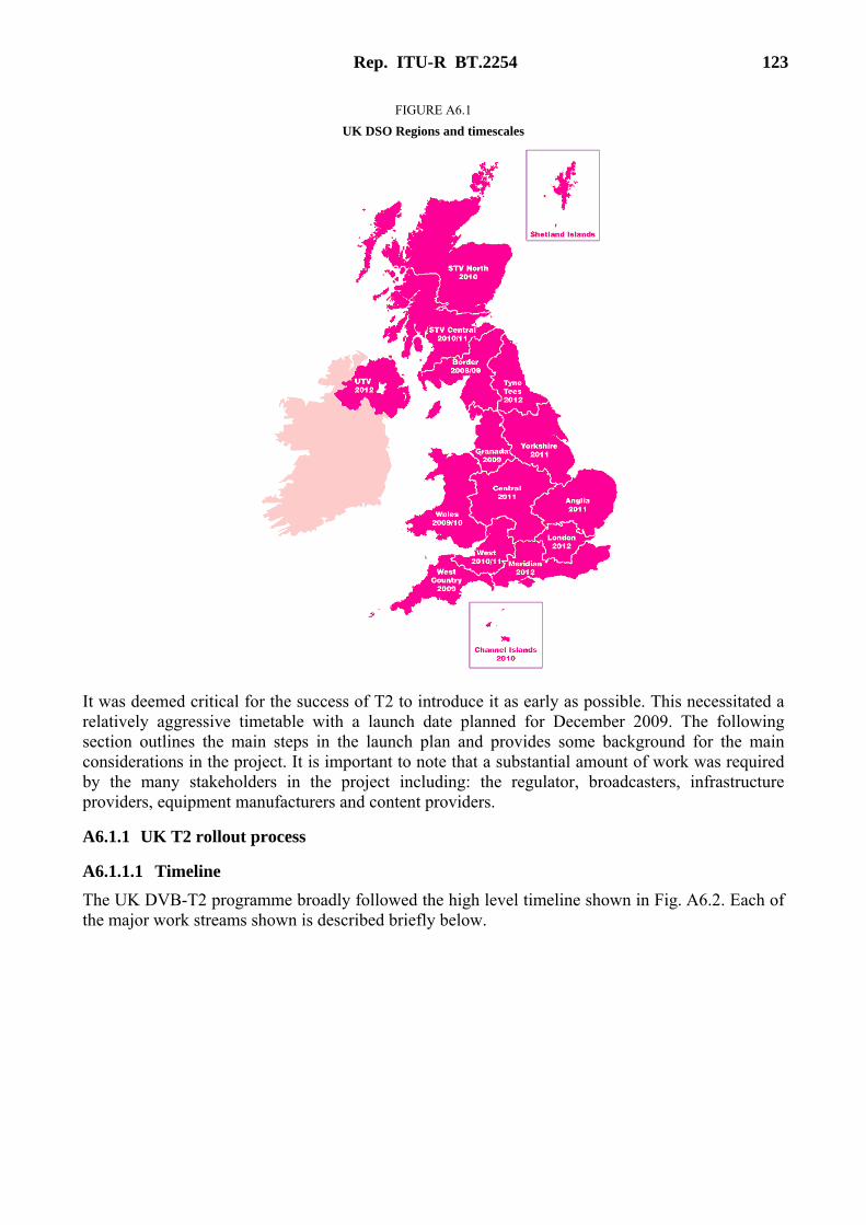
Rep. ITU-R BT.2254 123
FIGURE A6.1
UK DSO Regions and timescales
It was deemed critical for the success of T2 to introduce it as early as possible. This necessitated a relatively aggressive timetable with a launch date planned for December 2009. The following section outlines the main steps in the launch plan and provides some background for the main considerations in the project. It is important to note that a substantial amount of work was required by the many stakeholders in the project including: the regulator, broadcasters, infrastructure providers, equipment manufacturers and content providers.
A6.1.1 UK T2 rollout process
A6.1.1.1 Timeline
The UK DVB-T2 programme broadly followed the high level timeline shown in Fig. A6.2. Each of the major work streams shown is described briefly below.
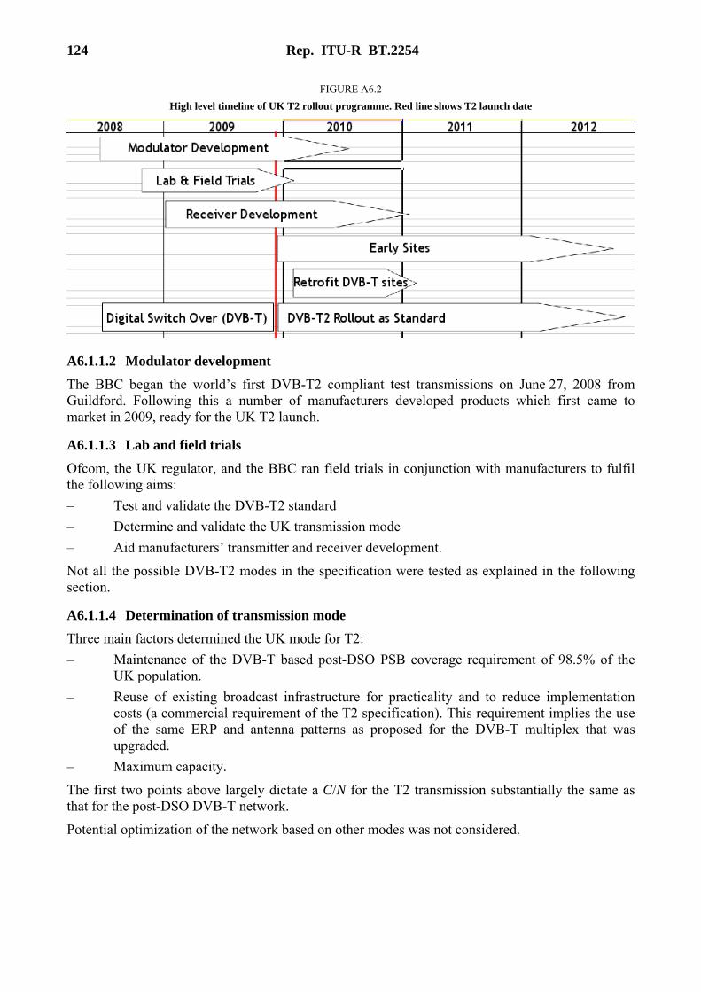
124 Rep. ITU-R BT.2254
FIGURE A6.2
High level timeline of UK T2 rollout programme. Red line shows T2 launch date
A6.1.1.2 Modulator development
The BBC began the world’s first DVB-T2 compliant test transmissions on June 27, 2008 from Guildford. Following this a number of manufacturers developed products which first came to market in 2009, ready for the UK T2 launch.
A6.1.1.3 Lab and field trials
Ofcom, the UK regulator, and the BBC ran field trials in conjunction with manufacturers to fulfil the following aims:
– Test and validate the DVB-T2 standard
– Determine and validate the UK transmission mode
– Aid manufacturers’ transmitter and receiver development.
Not all the possible DVB-T2 modes in the specification were tested as explained in the following section.
A6.1.1.4 Determination of transmission mode
Three main factors determined the UK mode for T2:
– Maintenance of the DVB-T based post-DSO PSB coverage requirement of 98.5% of the UK population.
– Reuse of existing broadcast infrastructure for practicality and to reduce implementation costs (a commercial requirement of the T2 specification). This requirement implies the use of the same ERP and antenna patterns as proposed for the DVB-T multiplex that was upgraded.
– Maximum capacity.
The first two points above largely dictate a C/N for the T2 transmission substantially the same as that for the post-DSO DVB-T network.
Potential optimization of the network based on other modes was not considered.
Rep. ITU-R BT.2254 125
A6.1.1.5 Receivers
The UK stakeholders developed a minimum receiver specification for:
– Set top Boxes
– Integrated Digital TVs
– Digital Television Recorders.
The DTG HD D-Book version 6 (March 2009) initially specified the technical system for use within the UK. Subsequent versions have since been released.
The UK broadcasters worked closely with a number of manufacturers to develop DVB-T2 products for launch in late 2009.
A6.1.1.6 Early sites
It is apparent from Fig. A6.1 that some key population areas would not receive the HD services until late in the DSO programme, with London planned to switch in 2012.
To increase the consumer market for receivers and to aid a successful launch, five “early” T2 services were launched in the following key cities covering approximately seven million households.
London
Glasgow and Edinburgh
Leeds/York
Birmingham
Newcastle, Sunderland, Middlesbrough.
Furthermore, the following significant sporting events occur before HD services would be available in some of the above regions if no ‘early’ sites were introduced. Providing large cities with HD for these events is likely to increase T2 uptake.
Football World Cup (June/July 2010)
Rugby World Cup (September/October 2011)
London Olympics (July 2012)
A6.1.1.7 Integration of T2 into the DSO programme and retrofit
The T2 launch began part-way through the pre-determined DVB-T rollout, meaning that some areas in the UK were entirely switched over to DVB-T by the time DVB-T2 was first launched, while others had a mixture of the pre-switchover analogue and low power DVB-T networks.
Beginning with the Granada region in late 2009, DVB-T2 was incorporated into the DSO programme and one PSB multiplex has since been ‘rolled out’ with T2 as standard. Managing to do this at such an early stage in the DSO programme significantly simplified the consumer message and rapidly began growing the consumer market.
It was also necessary to undertake a retro-fit programme to upgrade to T2 the areas of the UK such as the West Country that had already switched over and were operating as DVB-T only. This process was completed with minimal change and disruption to the DVB-T network as it primarily involved replacing the existing DVB-T modulator to the newer DVB-T2 version.
To achieve these goals in a short time-frame, a substantial amount of work has been undertaken by the many stakeholders in the project including the regulator, broadcasters, infrastructure providers and equipment manufacturers.
126 Rep. ITU-R BT.2254
A6.1.1.8 Re-transmitters and transposers
The regenerative relays in the DVB-T network require replacement or upgrade to make them suitable for DVB-T2. A substantial portion of the DVB-T transposer network has continued to operate correctly with a DVB-T2 signal without modification, although some changes will be necessary to maintain the monitoring/alarm systems.
A6.1.1.9 SFNs
The UK network makes use of medium power SFNs in a small number of cases. One T2 Gateway is needed for each SFN to create the Management Interface (T2-MI) stream that enables the SFNs to work correctly. These devices were not required for DVB-T. The primary SFNs have been implemented and are operational. They have been found to operate as expected.
A6.2 Introduction of DVB-T2 in Finland
In VHF there are three national multiplexes dedicated to DVB-T2 broadcasting and all the network licences have been granted to the network operator DNA. In March 2012 three DVB-T2 HDTV multiplexes cover over 80% of the population. DNA is building the networks mainly on telecom sites with lower power transmitters. DNA operates three DVB-T2 multiplexes with network parameters: 32k, 256-QAM, CR 4/5, GI 19/256.
In UHF two DVB-T2 network licences (one national and one regional) have been granted to the network operator Anvia and the transmissions were started in February 2011. In March 2012 the national DVB-T2 HDTV multiplex covers over 60% of the population and the regional multiplex covers Helsinki Metropolitan Area. Anvia is using the tall masts of Digita with high power transmitters. Anvia operates two DVB-T2 multiplexes with network parameters: 32k ext., 256-QAM, CR 4/5, GI 1/32.
In UHF Digita already operates four national DVB-T multiplexes: two covering about 100%, one covering about 95% and one covering about 90% of the population. In UHF DVB-H transmissions were closed down in March 2012 and Digita is allowed to convert the DVB-H network to the DVB-T2 network. In April 2012 the national DVB-T2 HDTV multiplex will cover about 85% of the population. Digita will operate the DVB-T2 multiplex with network parameters: 8k ext., 64-QAM, CR 4/5, GI 1/8.
Furthermore in UHF there will be one national DVB-T2 multiplex to cover about 80% of the population. The network licence will be granted in the near future.
A6.3 Introduction of DVB-T2 in Sweden
HDTV was launched in the terrestrial network in Sweden on 1st November 2010. Nine HDTV programmes were licenced, offering a mixture of existing programmes (simulcast SD & HD) and new programmes (HD exclusively). The public service broadcaster “Sveriges Television” has been awarded a licence for two of its programmes (simulcast with SD).
One of the nine licences was returned and in February 2012 the Swedish Broadcasting Authority received 26 new applications for the licence. There is a possibility of either one HDTV programme service or three SDTV programme services being awarded.
The programmes are transmitted in two multiplexes, Multiplex 6 and 7, both using DVB-T2 MPEG-4. Multiplex 6 uses UHF frequencies only and will carry five programmes, while Multiplex 7 uses both UHF and VHF frequencies. For the UHF transmissions, the extended bandwidth mode is used. For VHF this feature is not possible without exceeding the spectrum mask. Therefore the normal bandwidth mode is used for the VHF transmissions. Because of the slightly lower data rate possible for a 7 MHz channel and the normal bandwidth mode, the seventh
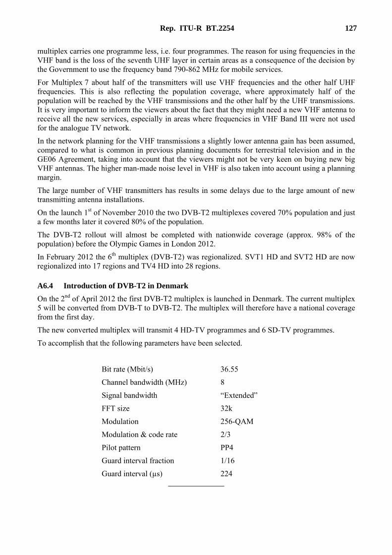
Rep. ITU-R BT.2254 127
multiplex carries one programme less, i.e. four programmes. The reason for using frequencies in the VHF band is the loss of the seventh UHF layer in certain areas as a consequence of the decision by the Government to use the frequency band 790-862 MHz for mobile services.
For Multiplex 7 about half of the transmitters will use VHF frequencies and the other half UHF frequencies. This is also reflecting the population coverage, where approximately half of the population will be reached by the VHF transmissions and the other half by the UHF transmissions. It is very important to inform the viewers about the fact that they might need a new VHF antenna to receive all the new services, especially in areas where frequencies in VHF Band III were not used for the analogue TV network.
In the network planning for the VHF transmissions a slightly lower antenna gain has been assumed, compared to what is common in previous planning documents for terrestrial television and in the GE06 Agreement, taking into account that the viewers might not be very keen on buying new big VHF antennas. The higher man-made noise level in VHF is also taken into account using a planning margin.
The large number of VHF transmitters has results in some delays due to the large amount of new transmitting antenna installations.
On the launch 1st of November 2010 the two DVB-T2 multiplexes covered 70% population and just a few months later it covered 80% of the population.
The DVB-T2 rollout will almost be completed with nationwide coverage (approx. 98% of the population) before the Olympic Games in London 2012.
In February 2012 the 6th multiplex (DVB-T2) was regionalized. SVT1 HD and SVT2 HD are now regionalized into 17 regions and TV4 HD into 28 regions.
A6.4 Introduction of DVB-T2 in Denmark
On the 2nd of April 2012 the first DVB-T2 multiplex is launched in Denmark. The current multiplex 5 will be converted from DVB-T to DVB-T2. The multiplex will therefore have a national coverage from the first day.
The new converted multiplex will transmit 4 HD-TV programmes and 6 SD-TV programmes.
To accomplish that the following parameters have been selected.
Bit rate (Mbit/s) 36.55
Channel bandwidth (MHz) 8
Signal bandwidth “Extended”
FFT size 32k
Modulation 256-QAM
Modulation & code rate 2/3
Pilot pattern PP4
Guard interval fraction 1/16
Guard interval (µs) 224