fpga enhanced surveillence techniques -...
TRANSCRIPT
FPGA ENHANCED SURVEILLENCE TECHNIQUES
by
Brian Coulson Heflin
B.A., University of Colorado at Colorado Springs, 2006
A thesis submitted to the Graduate Faculty of the
University of Colorado at Colorado Springs
in partial fulfillment of the
requirements for the degree of
Masters of Science
Department of Electrical and Computer Engineering
EAS_ECE_2008_004
This thesis for Master of Science degree by
Brian C. Heflin
has been approved for the
Department of Electrical and Computer Engineering
by
__________________________
Chia-Jiu Wang, Chair
__________________________
Terrence E. Boult
__________________________
Ramaswami Dandapani
________________
Date
Brian C. Heflin (M.S., Electrical and Computer Engineering)
FPGA Enhanced Surveillance Techniques
Thesis directed by Professor Chia-Jiu “Charlie” Wang
This thesis presents the theory, development and the simulation results for
a target detection and tracking system designed around a Virtex 4 FX FPGA.
The chosen target detection method is based on the subtraction of a reference
background from the current image obtained from the camera sensor.
Additionally, a comparison of different target detection and tracking algorithms
that use the background subtraction method for target detection is also
presented. Portions of the implemented FPGA accelerated target detection and
tracking system are based on the Lehigh Omnidirectional Tracking System
(LOTS) tracking system developed at Lehigh University under the guidance of
Dr. Terry Boult. The FPGA modules implemented the target detection, reference
background model and per pixel threshold updates, and the reduced resolution
“parent” image used the in target tracking algorithm. Xilinx simulation results are
shown for all of the implemented HDL modules. Finally, Xilinx map and post
place and route timing results are presented to show that the system can operate
with an input clock frequency of 200 MHz.

To my wife and son,
Jennifer and Coleson Heflin

iv
Acknowledgements
First, I would like to give thanks to my thesis committee chairman Dr. Chia-Jiu
(Charlie) Wang. I met Dr. Wang early in my undergraduate program and feel that
his knowledge and support was the key to my educational development and my
success in my Electrical Engineering curriculum.
I would also like to show my gratitude to Dr. Terrance E. Boult for his
assistance, patience, and guidance throughout my thesis research. I would also
like to extend my thanks to him for his comments and ideas during our graduate
meetings.
I also wish to show my appreciation to Michael D. Ciletti. His knowledge and
insights to the Verilog HDL language, and algorithm development for FPGAs is
exceptional. I feel honored and privileged to have been his student.
Finally, I would like to thank the School of Engineering and Applied Sciences
and the Electrical Engineering department chair Dr. T.S. Kalkur for giving me the
opportunity to perform the role as associate professor for the Spring 2008 Rapid
Prototyping with FPGAs class.
Table of Contents
List of Tables…………………………………………………………..vii
List of Figures…………………………………………………………....x
CHAPTER
I. INTRODUCTION………………………………………………..1
1.1 Visual Surveillance Fundamentals…………………..…….……2
1.2 Basic Background Subtraction…...……………………..………3
1.3 Purpose and Scope of the Study……………...………..………4
1.4 Arrangement of Thesis…………………………………………..5
1.5 Data / Other Limitations………………………………………….6
II. REVIEW OF THE LITERATURE……………………………..8
2.1 Introduction………………………………………………………..8
2.2 W4 Algorithm………………………………………………………8
2.2.1 W4 Background Modeling and Foreground Pixel Detection…………………………………………………...8
2.2.2 Tracking with the W4 Algorithm…………………………...9
2.3 Single Gaussian Model/Pfinder System………………………12
2.3.1 Target Detection using a Pfinder ……………………….12 2.3.2 Target Tracking using Pfinder …………………………..13
2.3 Adaptive Mixture of Gaussians………………………………...14
2.4 LOTS……………………………………………………………...15
2.4.1 Background Subtraction………………………………….16
2.4.2 Pixel Thresholding…………………………….…………..19
2.4.3 QCC………………………………………………………...21
2.4.4 Cleaning Regions…………………………………………23
2.4.5 Tracking with LOTS……………………………………….25
2.5 SUMMARY OF ALGORITHMS………………………………..25
III. METHODOLOGY…………..………………………………..29
3.1 FPGA Based Methodology and Architecture Introduction…..29
3.2 Background Subtraction/Pixel Thresholding HDL Modules...31
3.2.1 Background Subtraction Controller HDL Module………32
3.2.2 Background Subtraction Data Path……………………..37
3.3 16x16 Reduced Target Map……………………………………43
3.3.1 16x16 Reduced Target Map Controller…………………44
3.3.2 16x16 Reduced Target Map Datapath………………….48
3.4 TARGET MAP FILTER HDL Module………………………….50
3.4.1 TARGET MAP FILTER Controller……………………….50
3.4.2 Target Map Filter Datapath………………………………53
IV. Simulation/Synthesis Results……….…………….………..56
4.1 Simulation Introduction…………………………………………56
4.2 Background and Threshold Initialization……………………...57 4.3 Simulation Results for the Background Subtraction HDL
Modules…………………………………………………………..60
4.3.1 Experiments with FRAME 870…………………………..60
4.3.2 Experiments with FRAME 911…………………………..63
4.3.3 Simulation Results for the Target Map HDL Modules..66
4.3.4 Simulation Results for the Target Filter HDL Modules…………………………………………………67
4.4 QCC Results……………………………………………………..68
4.5 Discussion of Simulation Results……………………………...72
4.5.1 Simulation Results For the Target Map HDL Modules..74
4.5.2 Simulation of Target Map Filter HDL Modules…………74
4.6 Xilinx XST Synthesis results …………………………………..75
4.6.1 Xilinx XST Synthesis Summary………………………….76
V. CONCLUSION……...………………………………………...78
BIBLIOGRAPHY………………………………………………..80
APPENDIX
A. Synthesis, Map, Place and Route and Static Timing Report……………………………………………….....81
B. Verilog HDL Code……………………………………130
vii
List of Tables
TABLE
2.1. Summary of the 4 Target Detection and Tracking Algorithms……………….25
2.2. Results of [6] for the 4 Target Detection and Tracking Algorithms………….26 3.1. Truth Table for Embedded Update Flags………………………………………31 3.2. The Inputs to the Background Subtraction Controller
module………………………………………………………………..…………..33 3.3. The outputs of the Background Subtraction Controller
module…………………………………………………………………….………33 3.4. Control Signals Asserted at Each State Background Subtraction
Controller……………………………………………………………………………37 3.5. The Inputs to the Background Subtraction Data Path Module……………....38 3.6. The Outputs of the Background Subtraction Data Path Module…………….40 3.7. Truth Table for the 6-bit map_inc Value………………………………………..43 3.8. The Inputs to the 16x16 Reduced Target Map Controller Module…………..44 3.9. The Outputs to the 16x16 Reduced Target Map Controller Module………..44 3.10. Control Signals Asserted at Each State 16x16 Reduced Target Map
Controller………………………………………………….………………………47 . 3.11. The Inputs to 16x16 Reduced Target Map Data Path Module……………..48
3.12. The Outputs of the 16x16 Reduced Target Map Data Path Module………49 3.13. The inputs to the Target Map Filter controller module are………………….51 3.14. The Outputs of the Target Map Filter controller module……………………51 3.15. Control Signals Asserted at Each State 16x16 Reduced Target Map
Filter…………………………………………………………………………….…51 3.16. The Inputs to Target Map Filter Data Path Module………………………….53
3.17. The Outputs of the Target Map Filter Data Path Module…………………...54 4.1. Two Background Reference Models……………………………………………57
4.2. Output Threshold Images for Both Initialization Techniques………………...59
4.3. Verilog HDL simulation results for Caviar Frame 870………………………..60
4.4. Verilog HDL simulation results for Caviar Frame 911………………………..63
4.5. Returned images from the QCC algorithm…………………………………….68
4.6. Frame Rate and Corresponding Frame Size for a MICRON MT9T001…….72
4.7. Logic That Did not Meet Timing and the Actions Taken to Allow the Design
to Run at 200 MHz……………………………………………………………….75
xi
List of Figures
FIGURE
1.1. Eight Major Stages In A Target Tracking System………………………………2
2.1. Example of Correlating Silhouette Edges to Track a Person Running……..10
2.2. Example of the W4 Locating Both Target’s Head, Torso, Hands and Feet..11
2.3. Example 24x24 Difference Image With It’s “parent” Image………………….22
3.1. Top Level Block Diagram for the FPGA Based Target Detection and Tracking System………………………………………………………………....30
3.2. ASM Chart for Background Subtraction Controller……………………………36 3.3. ASM Chart for 16x16 Reduced Target Map Controller……………………….46 3.4. ASM Chart for Target Map Filter Controller……………………………………52 4.1.Verilog HDL simulation results for the 16x16 reduced target map using a
constant map_inc value of 6’b010_010…………………………………………66 4.2. Verilog HDL Simulation Results for the 16x16 Reduced Target Map
Filter……………………………………………………………………………….67

CHAPTER 1
INTRODUCTION
CHAPTER 1
INTRODUCTION 1.1 Visual Surveillance Fundamentals
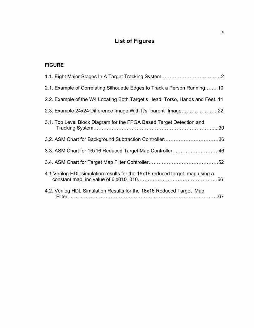
Visual surveillance algorithms have the job of detecting and tracking
targets. “From an architecture point of view, many visual surveillance systems
further decompose the problem resulting in to eight major stages: acquisition,
detection, grouping, tracking, filtering, classification, updating models, and
sensor control” [1]. Figure 1 below shows the block diagram of a target tracking
system.
Figure 1: Eight Major Stages In A Target Tracking System
The first two phases in the tracking of a target are the acquisition phase, where
the next image from a camera sensor is obtained and the detection phase where
a target or multiple targets are located within the image from the camera sensor.
The detector used in some target tracking systems is based on subtraction of a

reference background model from the image obtained from the sensor in the
acquisition phase.
1.2 Basic Background Subtraction
The detection phase uses background subtraction to detect changes in a
scene by computing the absolute difference, for every pixel, between the current
frame and a stored reference background frame . A difference image is
computed with equation (1.1):
(1.1)
where delta is the absolute difference the pixels of B and I. Next, if delta is
greater than a noise-based threshold , it is assumed that the pixel value
change is due to the presence of a target. Additionally, the choice of must be
high enough to ignore noise, but low enough to detect targets. There are two
primary approaches to reference modeling. The first is to adapt the reference
model over time by blending information and statistics extracted from many
images. The second method uses the two most recent frames for building the
reference image. After the detection phase has completed the next stage is the
grouping phase. The objective of the grouping phase is to assign a label to
pixels that are potentially a target pixel. “The most basic form of grouping is
simple connected components—the assignment of the same label to adjacent
pixels. Since this stage is early in the system, these uniformly labeled and well-
connected pixels regions are not necessarily deemed true targets. They are
often referred to with the less descriptive term blobs” [1]. The next phase is the

tracking phase. In the tracking phase each “blob” is related to blobs detected in
previous frames. An example of basic tracking would be to associate blobs from
the current frame to blobs from the previous frames that overlap or are within
some proximity of each other. After the tracking phase has completed the next
phase is the filtering phase. During the filtering phase more tests are performed
to ensure that the detected targets are really targets. The filtering process could
range from simple detection of targets without the minimum number of pixels or
area to more complex methods such as detecting changes in illumination, or
blobs that result from reflections or shadows. The optional classification phase
consists trying to further characterize detected targets. For example, a vehicle
recognition routine running in parallel with the target detection system could be
used to automatically detect and track vehicles of interest. The model update
phase consists of updating the internal models and parameters with new
information obtained from the most recent frame. “This might include adjusting
various thresholds, adjusting the background models, or updating internal system
variables. Since in many systems there can be several parameters per
pixel..[c]reating a system that both properly and rapidly self-adapts its internal
model is perhaps the largest challenge faced by visual surveillance community”
[1]. The final optional sensor control phase can incorporate the results of the
model update phase to adjust parameters of the video stream such as gain or
sensor integration time or it may activate a motor so a camera mounted to a
motor driven platform can follow the target.
1.3 Purpose of and Scope of Study
This thesis will document the implementation of an FPGA accelerated target
detection and tracking system for a stationary 3 Megapixel video camera.
Portions of the FPGA accelerated target detection and tracking system are based
on the Lehigh Omnidirectional Tracking System (LOTS) tracking system
developed at Lehigh University under the guidance of Dr. Terry Boult. The FPGA
modules will implement the target detection, reference background model and
per pixel threshold updates, and the reduced resolution “parent” image used the
in target tracking algorithm. I will also include a discussion of the complete
architecture for the target detection and tracking system including tracking,
filtering, and pixel grouping that will be executed by software running a PowerPC
embedded in a Virtex4 FX FPGA.
1.4 Arrangement of Thesis
Part I contains the introduction and the motivation for the thesis topic.
Furthermore, Part I is an introduction to the concepts of visual surveillance and
background subtraction. Part II is an examination of various target tracking
algorithms that use a target detector that is based on subtraction of a reference
background model from the image obtained from the sensor. Part III is a
complete examination of the individual Verilog HDL modules contained in the
target detection and tracking system. Additionally Part III contains a discussion of
the rest of the target tracking algorithm that will execute on a PowerPC running
on a Virtex 4 FPGA. Part IV contains my Verilog HDL simulation results for the

background subtraction/thresholding modules as well as the 16x16 reduced
resolution target map and target map filter HDL modules. Additionally, Part IV
contains a discussion of the Xilinx XSTsynthesis results, and timing benchmarks
for all of the implemented Verilog HDL modules. Part V is the thesis conclusion.
This section will be present recommendations and additional work that is needed.
Part VII is the Bibliography and Appendix. The Appendix contains all of the
Verilog code and the Xilinx synthesis, timing, map and post place and route
reports for all of the implemented Verilog HDL modules.
1.5 Data / Other Limitations
Since this thesis is the implementation of the hardware acceleration of the
target detection, reference background model updates, per pixel threshold
updates, and the reduced resolution “parent” image used in a target detection
and tracking system, the simulation data will be limited to the execution of the
background subtraction, pixel thresholding, reference background updating, and
formation of the 16x16 reduced resolution target map. The later parts of the
connect components tracking algorithm will be performed by software and is not
a part of the HDL simulation. However, the results from my simulations were
saved to data files and the connected components C++-code imported these
data files to generate the images shown in part IV.

CHAPTER II
REVIEW OF LITERATURE
CHAPTER 2
REVIEW OF LITERATURE
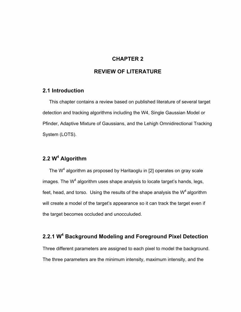
2.1 Introduction This chapter contains a review based on published literature of several target
detection and tracking algorithms including the W4, Single Gaussian Model or
Pfinder, Adaptive Mixture of Gaussians, and the Lehigh Omnidirectional Tracking
System (LOTS).
2.2 W4 Algorithm The W4 algorithm as proposed by Haritaoglu in [2] operates on gray scale
images. The W4 algorithm uses shape analysis to locate target’s hands, legs,
feet, head, and torso. Using the results of the shape analysis the W4 algorithm
will create a model of the target’s appearance so it can track the target even if
the target becomes occluded and unocculuded.
2.2.1 W4 Background Modeling and Foreground Pixel Detection
Three different parameters are assigned to each pixel to model the background.
The three parameters are the minimum intensity, maximum intensity, and the
maximum absolute difference in consecutive frames. The first step in the W4
algorithm is pixel thresholding. A pixel is considered a possible target if
(2.1) Where is the minimum intensity, and is the maximum intensity, and
is the maximum intensity difference. Unfortunately the resulting threshold
image contains a considerable amount of noise. Therefore, the next step is to
perform a region based noise cleaning that is comprised of an erosion operation
followed by a connected component analysis that removes regions with less than
50 pixels above threshold. The result of the connected component analysis is a
set of bounding boxes with target pixels. Next more morphological operations
comprised of dilatation and erosion are applied to the pixels inside of the boxes
and the final boxes are returned as targets.
2.2.2 Tracking with the W4 Algorithm
The goal of the W4 algorithm is to perform a fast and robust tracking algorithm.
The W4 algorithm is designed to track objects even if the first level of detection
does not segment multiple targets. “[The W4 algorithm] can determine whether a
foreground region contains multiple people and can segment the region into its
constituent people and track them. W4 can also determine whether people are
carrying objects, and can segment objects from their silhouettes, and construct
appearance models for them so they can be identified in subsequent frames. W4
can recognize events between people and objects, such as depositing an object,
exchanging bags, or removing an object” [2]. Next the W4 algorithm performs a
two stage motion estimation algorithm. First a preliminary calculation of the
object is performed to determine the initial displacement of the median between
the foreground region in the previous frame and current frame
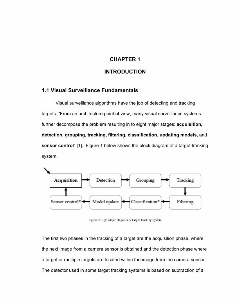
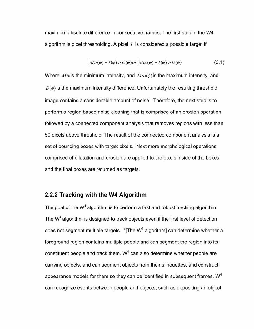
Next, “…the best match between previous silhouette edges and current
silhouette edges is found by correlating over a 5x3 displacement mask centered
at the initial displacement estimate”[3].. Figure 2.1 below shows an example of
correlating silhouette edges to track a person running.
Figure 2.1: Example of Correlating Silhouette Edges to Track a Person Running
The W4 algorithm also generates a temporal texture template for each target that
is being tracked using the average intensity of the corresponding foreground
pixels. Dynamic template matching can then be used to identify targets when
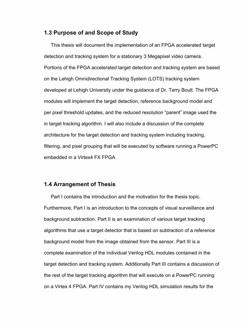
they become occluded and then unoccluded. Next the W4 algorithm locates the
target’s hands, feet, legs, head, and torso “Hands are located after torso by
finding extreme regions which are connect to the torso and which are outside of
torso…height of the bounding box of an object is taken as a height of the
cardboard model, then fixed vertical scales are used to find the approximate
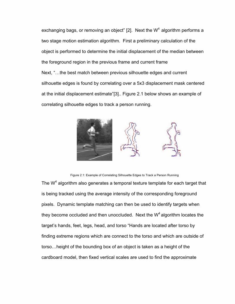
initial location of body parts” [3]. Figure 2.2 below shows an example of the W4
locating both targets head, torso, hands and feet.
Figure 2.2: Example of the W4 Locating Both Target’s Head, Torso, Hands and Feet
The target models are then tracked across multiple frames using a correlation
technique. “The estimated location of an template is calculated by global motion
g(t) of body and local motion l(t) of head (hands). The correlation results are
monitored during tracking to determine if the correlation is good enough to track
the parts. Changes in the correlation scores allow us to make a prediction about
whether a part is becoming occluded. When tracking fails, detection is re-
initialized subsequently with the static cardboard model”[3]. The W4 algorithm
can run at 25 Hz for 320×240 resolution images on a 400 MHz dual-Pentium II
PC.
2.3 Single Gaussian Model The Single Gaussian Model of Pfinder algorithm as proposed by Wren in [4] is
target detection and tracking system that also tries to interpret the target’s
behavior. “The system uses a multiclass statistical model of color and shape to
obtain a 2D representation of head and hands in a wide range of viewing
conditions. Pfinder has been successfully used in a wide range of applications
including wireless interfaces, video databases, and low-bandwidth coding” [4].
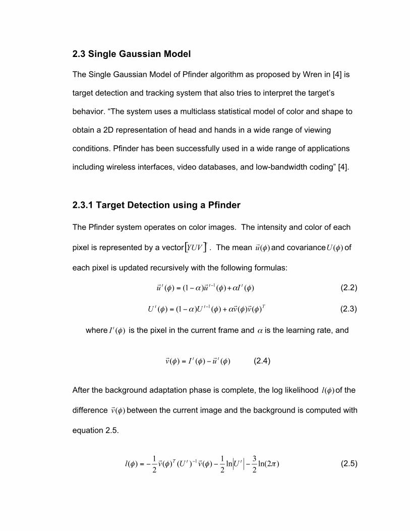
2.3.1 Target Detection using a Pfinder
The Pfinder system operates on color images. The intensity and color of each
pixel is represented by a vector . The mean and covariance of
each pixel is updated recursively with the following formulas:
(2.2)
(2.3)
where is the pixel in the current frame and is the learning rate, and
(2.4)
After the background adaptation phase is complete, the log likelihood of the
difference between the current image and the background is computed with
equation 2.5.
(2.5)
A pixel is classified as a potential target if else it is considered as part of
the background. Finally, the algorithm detects targets by performing connected
components on the non-background labeled pixels.
2.3.1 Target Tracking using Pfinder Once the Pfinder algorithmhas located a target it tries to build a more detailed
model. “A more detailed model of the user includes information about the
composition of the user. The same gaussian blobs that are used to classify the
image can also be useful as a model of the user” [5]. Next, the Pfinder system
tries to locate the head, feet, and hands of the target. Once the head, hands, and
feet have been located the system can track the target and can also identify if the
target is sitting, standing or pointing. The Pfinder algorithm can process 10
frames per second on an SGI indy with a 175Mhz R4400 CPU, and Vino Video
with a reduced fame size of (160x120).
2.3 Adaptive Mixture of Gaussians
In the adaptive mixture of Gaussians algorithm each pixel is modeled by a
mixture of K Gaussians:
(2.6)
where K = 3..5 or 4 in [6], “Furthermore is assumed that . The
background is updated as follows:
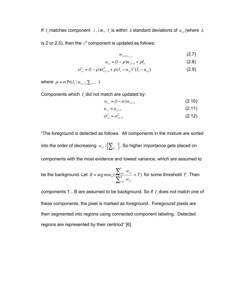
If matches component , i.e., is within standard deviations of (where
is 2 or 2.5), then the component is updated as follows:
(2.7) (2.8) (2.9)
where Components which did not match are updated by:
(2.10) (2.11) (2.12)
“The foreground is detected as follows. All components in the mixture are sorted
into the order of decreasing . So higher importance gets placed on
components with the most evidence and lowest variance, which are assumed to
be the background. Let for some threshold Then
components 1…B are assumed to be background. So if does not match one of
these components, the pixel is marked as foreground. Foreground pixels are
then segmented into regions using connected component labeling. Detected
regions are represented by their centriod” [6].
2.4 LOTS
The LOTS tracking system was developed at Lehigh University under the
guidance of Dr. Terry Boult. The area of application of the LOTS target detection
and tracking system is different from many other tracking systems. It was
designed to “track targets in a perimeter security type setting, i.e. outdoor
operation in moderate to high cover areas.” Some of the constrains and
implications for the LOTS system as presented in [7] are:
• The lighting is naturally varying. We must handle sunlight
filtered through trees and intermittent cloud cover.
• Targets use camouflage, thus it is unlikely that color will
add much information.
• Targets will be moving in areas with large amounts of
occlusion; finding/classifying outlines will be difficult.
Trees/brush/clouds all move. The system must have algorithms
to help distinguish these “insignificant” motions
from target motions.
• Many targets will move slowly (less than .01 pixel per
frame); some will be stationary for a two minutes or
more. Some will try very hard to blend into the motion
of the trees/brush. Therefore frame-to-frame differencing
is of limited value. Temporal adaptation schemes must
not add slow targets to the background.
• Targets will not, in general, be “upright” or isolated. Thus
we have not added “labeling” of targets based on simple
shape/scale/orientation models.
• Targets need to be detected quickly and when they are
still very small and distant, e.g. about 10-20 pixels on
target.
• Correlation, template matching, and related techniques
cannot be effectively used because of large amounts of
occlusion and because in a paraimage, image translation
is a very poor model; objects translating in the world undergo
rotation and non-linear scaling.
The LOTS target detection and tracking system has three distinctive features.
The first distinct feature is the use of multiple background reference models. The
system uses 3 background models. The second distinct feature of LOTS is the
speed that the system adapts its background models. The last distinct feature of
the LOTS target detection and tracking system system is the use of a per pixel
threshold with a high and low threshold.
2.4.1 Background Subtraction
As presented in [1] the LOTS system uses a three background models. At
time the primary background is represented by and the second
background by . The pixel intensity value is represented by , where
is the pixel index for a gray scale image. Additionally, in [1] is was
presumed that the input at time was closer to the primary background model
. The difference images are defined as:
(2.13)
(2.14)
and the variable , as the index with the smaller difference and as
the remaining index. In [1] they also allowed for a process to label the pixel as
being the the target set or in the nontarget set . The background models are
updated as follows:
(2.15)
Usually is smaller than . Additionally, the other background model is not
updated:
(2.16)
However, the LOTS system does not update every pixel in the background every
frame. Instead it reduces the rate at which the background is update so that the
multiplicative blending factor was at least 1/32. For example, an effective
integration factor with is achieved by adding 1/32 of the
new frame to the background every 1024th frame. “Given a target that differs from
a mid-gray background by 32 and a threshold of 16, the adaptation results in
requiring between 2 to 4096 frames for the target to become part of the
background” [8]. To further reduce the rate that the target pixels blend into the
reference background, pixels identified as “targets” have a smaller effective
integration factor. Initial analysis of the LOTS system showed that if the
background model was updated every frame, it became by far the most
computationally expensive component of the system since it requires a multiply,
add, and a shift operation. Therefore, for a faster implementation of the
reference background update a new update rule called the up-down, or the
conditional increment model was developed. Equation 2.17 below shows the
conditional increment model.
(2.17)
“The most important drawback to the conditional increment model is that if a
target is mislabeled, the system does not “blend” it in significantly; it does not
matter if the target is nearly the same or distant in grey values, the update is
constant. Since the primary goal of this aspect of the system is to update the
background to handle diurnal lighting changes (which should be slow), using a
scaled difference does not seem justified. Rather than always blending quickly,
LOTS has a separate rapid lighting change detection subsystem that temporarily
changes the system behavior when large (i.e. non-diurnal) lighting changes
occur. When strong lighting changes are detected, the current system
temporarily increases its thresholds while also switching to a larger alpha-
blending-based algorithm to more quickly adapt away the changes. The switch
between the modes is automatic and based on rate of growth in a number of
pixels labeled as targets. If the growth rate is very radical, such as might occur if
an adversary shines a laser directly into the imaging system, the system reports
it immediately and tries again on the next frame. With this separate lighting
model change technique, the system can maintain high sensitivity while
maintaining robustness” [1]. Since the primary and secondary backgrounds are
updated with temporal blending to allow them to track slow lighting changes, the
blending can result in persistent false alarms and targets leaving “ghosts”. To
deal with these issues the system has a third background reference image,
called the old-image that is used in the cleaning phase of the tracking algorithm.
Unlike the primary and secondary backgrounds the old-image is not updated with
an incremental or blending model instead it is an exact copy of an input frame
from between 9000-18000 frames ago. Furthermore, regions that contain targets
when the old-image is formed are marked as non targets.
2.4.2 Pixel Thresholding
The LOTS tracking system also utilizes multiple pixel thresholds. The first
threshold is a global threshold. The global threshold is used to deal with the
camera gain noise and can be adjusted while the system is running. The second
threshold is a per-pixel threshold. The per-pixel threshold “…attempts to account
for the inherent spatial variability of the scene intensity at the pixel, e.g. points

near edges will have higher variability because of small changes in the imaging
situation can cause large intensity changes” [7]. Similarly to the multiple
background models, the per-pixel threshold is not updated every frame. The
adaptation scheme slowly decreases the threshold for missed pixels. A missed
label means that the pixel was not above threshold but is part of a detected
region. If a pixel is detected the threshold remains constant. A detected label
signifies that the pixel corresponds to a detected region. Finally, if the pixel
becomes an insertion due to noisy pixels or if the threshold is to low it is
increased. An insertion label means that the pixel was above threshold but not
part of a detected region. Equation 2.18 below shows a summary of the threshold
updating scheme.
(2.18)
Since there should only be a small growth in the number of pixels that are above
threshold, the system contains a counter for the number of pixels that are above
threshold. If the growth or number of pixels is too large, the system assumes it is
probably a rapid lighting change or a radical camera motion. “The system
attempts to handle radical growth by presuming it to be a rapid lighting change
and temporarily increases both the global threshold and the allowed growth rate.
This attempt to increase the thresholds is tried twice. If it is successful in
reducing the growth, we proceed as usual except we force an update of non-
target regions with a blending factor much larger than usual. If after raising the
threshold a few times we still detect that the number of pixels differing from the
backgrounds is growing
too fast then we presume the growth must be because of camera motion. To
handle camera motion we:
1. skip tracking for this frame,
2. then increase the allowed growth rate suspending tracking for the next frame
3. call for an absolute update (all pixels are updated). If camera-motion events
are considered significant, we also inform the user” [7].
2.4.3 QCC
After the background subtraction and thresholding is complete the pixels
that are above high and/or low threshold need to be grouped into regions. A
connected component labeling technique called Quasi-Connected Components
(QCC) is used to not only to label the regions but also to discard small noise
regions in an efficient manner suitable for implementation onto a FPGA.
Furthermore, the processing time for the QCC algorithm is reduced by three
techniques. The first technique is that only the part of the row between the
leftmost pixel above threshold and the rightmost pixel above threshold is
processed. The second technique is that the connectivity analysis uses a
modified union-find data structure to allow very fast association of regions. The
last technique is the QCC algorithm operates on a reduced resolution or “parent”
image. Figure 2.3 below shows an example 24x24 difference image with it’s
“parent” image below.

Figure 2.3: Example 24x24 Difference Image With It’s “parent” Image
For example, during the initial phase of QCC the 24x24 difference image shown
in figure 2.3 could be reduced by a factor of 4 in each direction, as shown in the
6x6 image to the lower left of the difference image. “Because of its relation to
similar concepts in multi-resolution processing, this is generally called the parent
image, where each parent pixel has multiple child pixels that contribute to it. The
value of each parent pixel in this parent images is, initially, a count (area) of how
many pixels were above the low threshold and how many were above the high
threshold” [1]. The original LOTS implementation used a 32-bit integer to hold the
number of pixels above the high and low threshold in a 4x4 block. Where the
upper 16 bits contains the count of the number of pixels above the high threshold
and the lower 16-bits is the count of the number of pixels above the low threshold
but below the high threshold. In a 4x4 block the number of pixels that could be
above high and/or low threshold could be 16. “Because of limited ranges, this
allows a single 32-bit addition to combine both counts without the danger of
overflow” [1]. In figure 2.3 on the previous page the shaded pixels are above the
low threshold and the pixels that are patterned are above the high and low
thresholds. The difference image in figure 2.3 shows regions with pixels that are
above the high and/or low threshold. The upper left region contains 5 pixels
above threshold, one of which is above the high threshold. The lower left region
contains 13 pixels above the low threshold only. The middle right region contains
21 pixels above threshold, 4 of which are above the high threshold. The value of
bottom green pixel in the bottom left parent image of figure 2.3, has a value of 6
since it is the parent of 6 pixels above the low threshold and 0 above the high
threshold. The second yellow pixel is associated with 2 pixels above the low
threshold, and 1 pixel above the high threshold. Therefore it has the value
0x0100 + 0x0002 = 0x0102 (258 decimal).
2.4.4 Cleaning Regions
The next phase in the QCC algorithm is to clean the detected regions with
three different algorithms: size, lighting normalization and unoccluded region.
The first algorithm uses area thresholds to remove noise regions. The lighting
normalization and unoccluded region cleaning algorithms makes use of
normalized intensity data from the input image, the primary background, and the
third background or “old image”. The second cleaning or lighting normalization
algorithm tries to account for local lighting variations by reperforming the pixel
thresholding procedure using a normalized background intensity. The
normalized background intensity is computed for each region so it can handle
sun light filtered through a tree or small cloud patches in the scene.
The third cleaning phase or unoccluded region cleaning algorithm is used “…to
see if it is a region where a moving target has disoccluded the background, i.e.
handling a “ghost” image. This is done by doing a thresholding with-hysteresis
comparison against an intensity normalized version of the old image”[7].
2.4.5 Tracking with LOTS
The tracking phase of the QCC algorithm tries to connect target regions
detected in the current frame to targets detected in prior frames. First the QCC
algorithm uses the current “parent” image as well as the “parent” image from the
past frame to associate blobs from the previous frame. Blobs that are connected
in space-time are labeled with the same label they had in the past frame. Next
the algorithm tries to merge new regions with other regions in close proximity that
have strong temporal associations. The QCC algorithm will also connect new
regions with regions that were not in the previous frame but had been tracked in
earlier frames. “For regions that are “tracked”, we maintain information on their
position (image coordinates and 3D world coordinates), current and average
velocity (image and world), their size, length of time tracked, path (most recent
100 positions), positions avert to their most recent intensity distributions, and
their confidence measures” [7].
2.5 SUMMARY OF ALGORITHMS
In summary, the Pfinder algorithm and the adaptive mixture of gaussian
MOG algorithms are very computationally intensive and the system parameters
require extensive tuning. The algorithms are also very sensitive to changes in
illumination such as the sun going behind a cloud. Additionally, the longer that
the scene remains static the smaller the variances of the background will become
and a sudden change in illumination will cause the entire frame to turn into a
target. The W4 algorithm is less computationally expensive than the Pfinder
algorithm or adaptive MOG algorithms however, the W4 algorithm is extremely
sensitive to motion of background objects camera jitter, and illumination changes.
The LOTS algorithm is also less computationally expensive than the Pfinder or
adaptive MOG algorithms and it can also account for sudden changes in
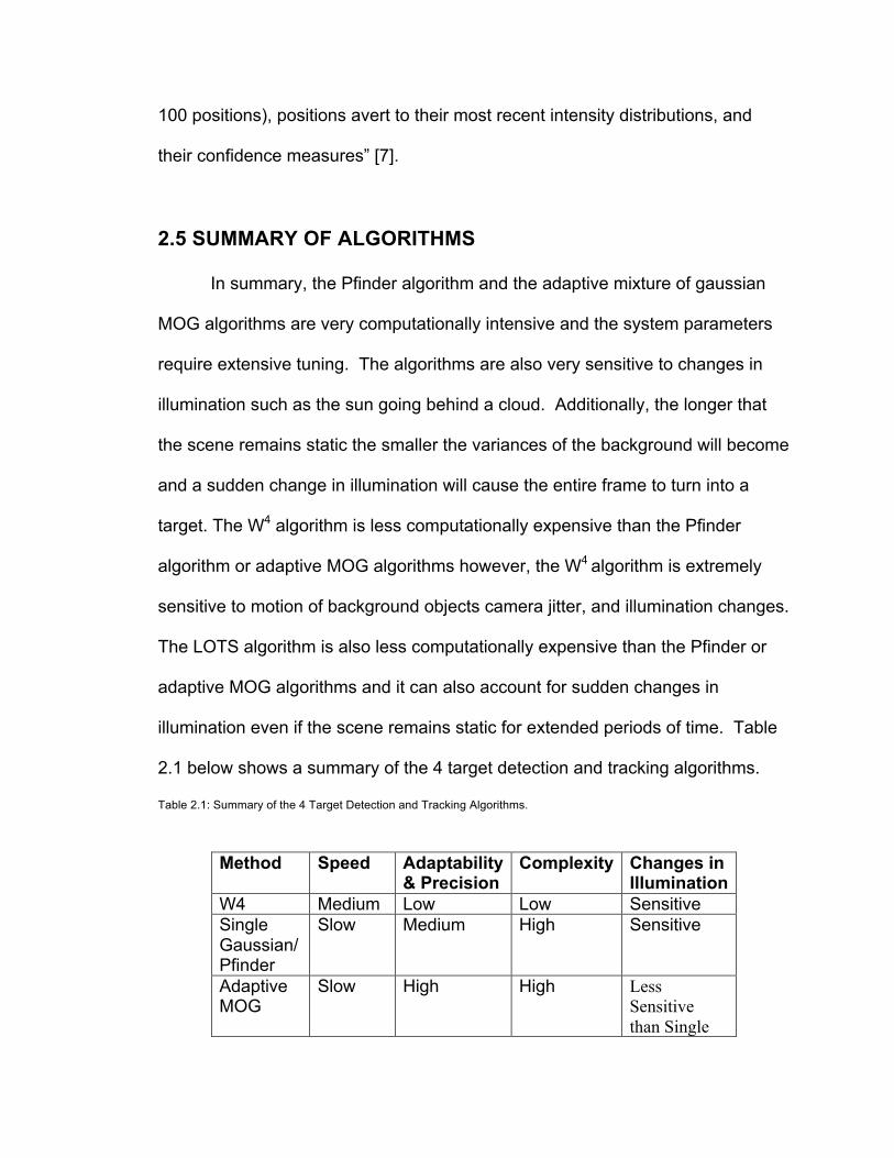
illumination even if the scene remains static for extended periods of time. Table
2.1 below shows a summary of the 4 target detection and tracking algorithms.
Table 2.1: Summary of the 4 Target Detection and Tracking Algorithms.
Method Speed Adaptability & Precision
Complexity Changes in Illumination
W4 Medium Low Low Sensitive Single Gaussian/ Pfinder
Slow Medium High Sensitive
Adaptive MOG
Slow High High Less Sensitive than Single

Gaussian LOTS Fast High Low Moderately
Sensitive
Additionally, in [6] the authors compared the various target detection and tracking
algorithms against each other using a performance measure called Tracker
Detection Rate (TRDR) and False Alarm Rate (Far).
Where is a true positive detection, is an insertion or false positive, and
is a messed target or false negative. Table 2.2 below shows the results of
their experiments for the 4 target detection and tracking algorithms from the
previous section.
Table 2.2: Results of [6] for the 4 Target Detection and Tracking Algorithms
From table 2.2 if can be seen that the LOTS algorithm had the highest target
detection rate and the second lowest false alarm rate as compared to the other 3
algorithms. While the Pfinder, MOG and W4 algorithms can be used to detect
and track targets, for an FPGA implementation the computational complexity of
the 3 algorithms out weighs the performance as compared to the LOTS
algorithm. Additionally, the LOTS algorithm can achieve better performance while
using only fixed point operations that can readily implemented onto a FPGA.
While the W4 is less complex than the Pfinder and MOG algorithms it still
requires more complex dilation and erosion operations on the pixel data as
compared to the LOTS algorithm. Furthermore the SGM, MGM and W4
algorithms are extremely sensitive to motion of background objects camera jitter,
and illumination changes while the LOTS algorithm has routines to account for
camera jitter, and illumination changes.

CHAPTER III
METHODOLOGY
CHAPTER 3
METHODOLOGY
3.1 FPGA Based Methodology and Architecture Introduction
The FPGA based architecture for implementation the target detection and
tracking system consists of using the FPGA fabric for the preprocessing of the
data to include the background subtraction, background reference model
updates, pixel thresholding, and the forming the reduced resolution “parent”
image presented in section 2.4.3 in conjunction with using an embedded
PowerPC to perform the later steps of the target tracking using the QCC
algorithm. The FPGA based architecture will allow parts of the tracking system
to execute in parallel and at different clock frequencies if necessary. The
PowerPC and FPGA modules can transfer data through the use of the FPGA’s
embedded dual-port block ram. The PowerPC can be connected to a dual port
block ram controller that allows the C-code to access the block ram’s content
easily through the use of pointers to the block ram’s assigned address space.
Additionally, user created HDL modules known as pcores, that are attached to
the processor local bus or PLB bus will be used to read and write pixel data,
background model, and threshold data to the multiport-memory controller
input/output buffers. Then the multiport-memory controller will read and write the

data to the DDR SDRAM. Figure 3.1 below shows the top level block diagram for
the FPGA based target detection and tracking system.
Figure 3.1: Top Level Block Diagram for the FPGA Based Target Detection and Tracking System
3.2 Background Subtraction/Pixel Thresholding HDL Modules
The background subtraction HDL Module will accept 8-bit pixel data and
64-bit background and threshold data for processing. Since the reference
background data is only 32-bits for input every pixel this will allow the HDL
module to operate on two pixels in parallel. The output of the background
subtraction HDL Module is the map increment or map_inc value for the 16x16
reduced target map HDL modules and the updated reference background and
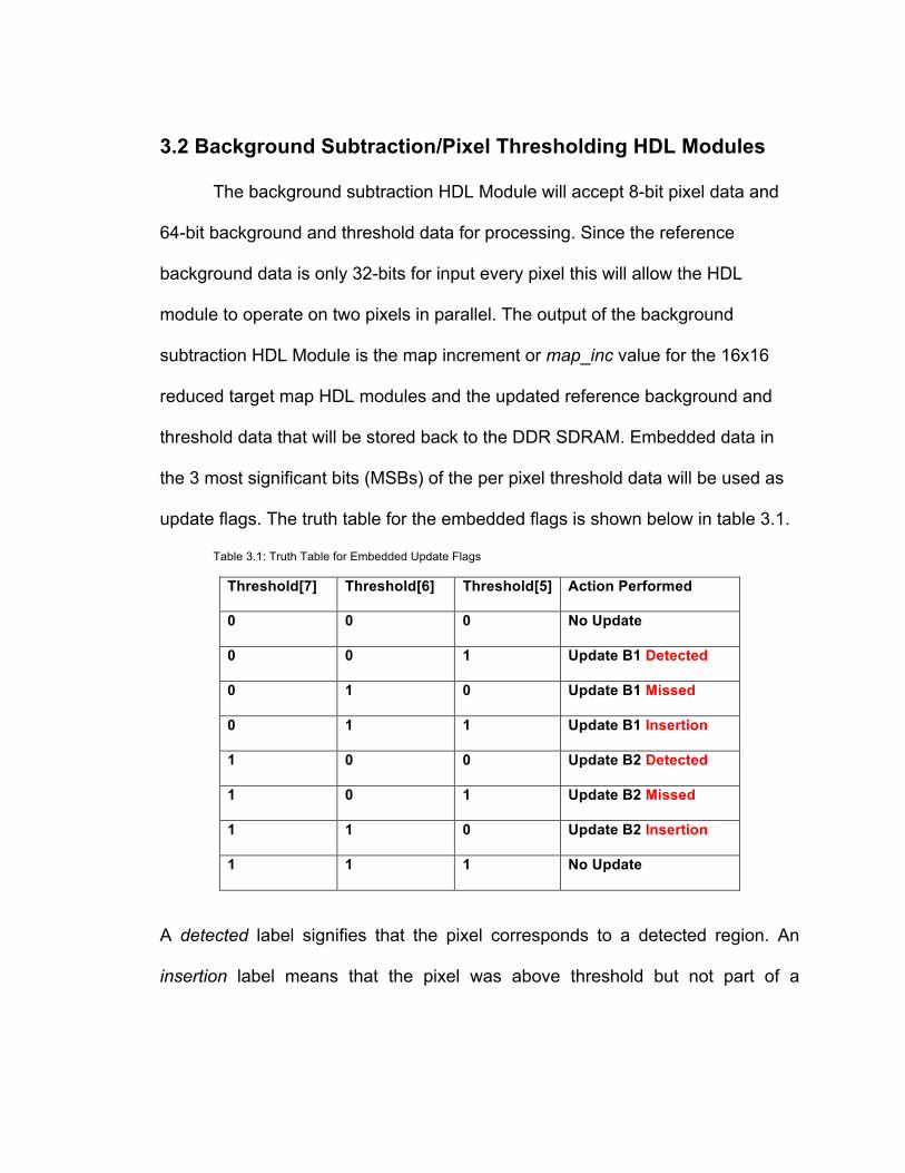
threshold data that will be stored back to the DDR SDRAM. Embedded data in
the 3 most significant bits (MSBs) of the per pixel threshold data will be used as
update flags. The truth table for the embedded flags is shown below in table 3.1.
Table 3.1: Truth Table for Embedded Update Flags
Threshold[7] Threshold[6] Threshold[5] Action Performed
0 0 0 No Update
0 0 1 Update B1 Detected
0 1 0 Update B1 Missed
0 1 1 Update B1 Insertion
1 0 0 Update B2 Detected
1 0 1 Update B2 Missed
1 1 0 Update B2 Insertion
1 1 1 No Update
A detected label signifies that the pixel corresponds to a detected region. An
insertion label means that the pixel was above threshold but not part of a
detected region. A missed label means that the pixel was not above threshold
but is part of a detected region.
3.2.1 Background Subtraction Controller HDL Module
The background subtraction controller HDL module is a finite state
machine (FSM) that will control the flow of pixel and reference background data
into the background subtraction datapath module for processing. Control signals
are sent from the background subtraction controller to the background
subtraction datapath to perform operations such as subtraction of the current
pixel data from the reference backgrounds and the reference background
updates. Additionally, at the end of every frame the controller will check the
number of pixels that were above the high and/or low threshold. If the number is
greater than a user defined value it is assumed that the change is due to a rapid
lighting change or radical camera motion. The background controller will handle
radical growth by first assuming that the growth is due to a rapid lighting change
and will increase the global threshold by 4 in addition to the allowed growth rate.
This technique is tried 2 times, if it is successful in reducing the growth, the
system will continue processing the input frames and update all non-target
regions with a slightly larger blending factor. If the previous technique fails it is
assumed that the radical growth is due to camera motion. The controller will
perform the following tasks:
1. Increase the allowed growth rate and suspend tracking for the next
frame
2. Call for an absolute update of all background reference pixels.
3. A flag or interrupt can be sent to the PowerPC to inform the user
that a camera motion event is taking place.
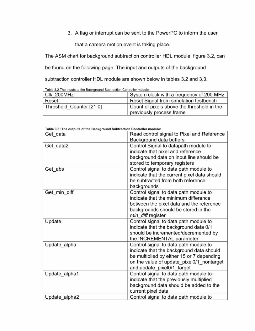
The ASM chart for background subtraction controller HDL module, figure 3.2, can
be found on the following page. The input and outputs of the background
subtraction controller HDL module are shown below in tables 3.2 and 3.3.
Table 3.2 The Inputs to the Background Subtraction Controller module:
Clk_200MHz System clock with a frequency of 200 MHz Reset Reset Signal from simulation testbench Threshold_Counter [21:0] Count of pixels above the threshold in the
previously process frame Table 3.3 :The outputs of the Background Subtraction Controller module: Get_data Read control signal to Pixel and Reference
Background data buffers Get_data2 Control Signal to datapath module to
indicate that pixel and reference background data on input line should be stored to temporary registers
Get_abs Control signal to data path module to indicate that the current pixel data should be subtracted from both reference backgrounds
Get_min_diff Control signal to data path module to indicate that the minimum difference between the pixel data and the reference backgrounds should be stored in the min_diff register
Update Control signal to data path module to indicate that the background data 0/1 should be incremented/decremented by the INCREMENTAL parameter
Update_alpha Control signal to data path module to indicate that the background data should be multiplied by either 15 or 7 depending on the value of update_pixel0/1_nontarget and update_pixel0/1_target
Update_alpha1 Control signal to data path module to indicate that the previously multiplied background data should be added to the current pixel data
Update_alpha2 Control signal to data path module to

indicate that the previously added data should be shifted by either 2 or 4 depending on the value of update_pixel0/1_nontarget and update_pixel0/1_target
Update_pixel0_nontarget Control signal to data path module to indicate that the reference background for pixel_0 should be updated this frame with nontarget parameters
Update_pixel0_target Control signal to data path module to indicate that the reference background for pixel_0 should be updated this frame with target parameters
Update_pixel1_nontarget Control signal to data path module to indicate that the reference background for pixel_1 should be updated this frame with nontarget parameters
Update_pixel1_target Control signal to data path module to indicate that the reference background for pixel_1 should be updated this frame with target parameters
Update_pixel0 Control signal to data path module to indicate that background_0 should be updated
Update_pixel1 Control signal to data path module to indicate that background_1 should be updated
Label Control signal to data path module to modify the update flag in background_1 and both map_inc values
Inc_SRAM_read_ptr Control signal to data path module to increment the read pointer to the pixel data and background reference data buffer
Inc_SRAM_write_ptr Control signal to data path module to increment the write pointer to the pixel data and background reference data buffer
Write_SRAM_Out Control signal to output buffers to write the current input data to the buffer
Output Control signal to data path module to output the updated background reference data and map_inc data
Temp_inc_global Control signal to data path module to indicate that the global threshold should be incremented by 4
Decrease_global_1x Control signal to data path module to indicate that the global threshold should be

decremented by 4 Decrease_global_2x Control signal to data path module to
indicate that the global threshold should be decremented by 8
Update_old_frame Control signal to data path module to indicate that the old frame reference data should be updated with the current pixel data
non_target_update Absolute_update Control signal to data path module to
indicate that all pixels should be updated this frame
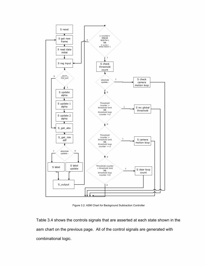
Figure 3.2: ASM Chart for Background Subtraction Controller
Table 3.4 shows the controls signals that are asserted at each state shown in the
asm chart on the previous page. All of the control signals are generated with
combinational logic.
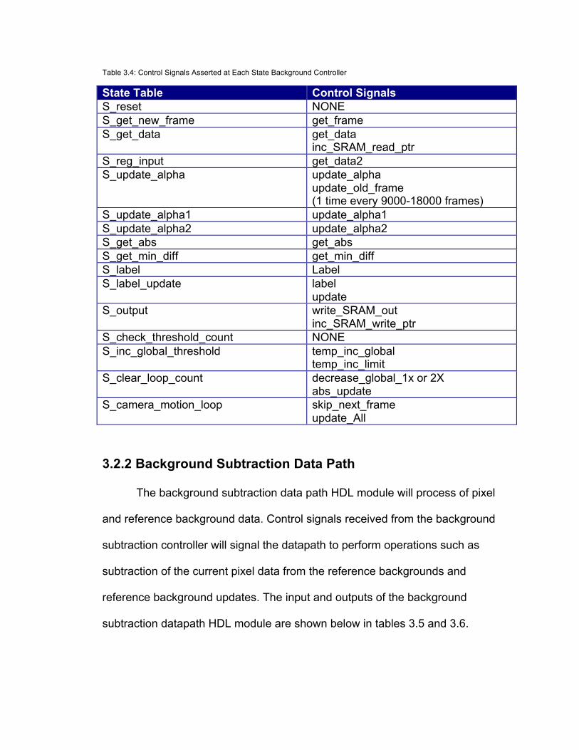
Table 3.4: Control Signals Asserted at Each State Background Controller
State Table Control Signals S_reset NONE S_get_new_frame get_frame S_get_data get_data
inc_SRAM_read_ptr S_reg_input get_data2 S_update_alpha update_alpha
update_old_frame (1 time every 9000-18000 frames)
S_update_alpha1 update_alpha1 S_update_alpha2 update_alpha2 S_get_abs get_abs S_get_min_diff get_min_diff S_label Label S_label_update label
update S_output write_SRAM_out
inc_SRAM_write_ptr S_check_threshold_count NONE S_inc_global_threshold temp_inc_global
temp_inc_limit S_clear_loop_count decrease_global_1x or 2X
abs_update S_camera_motion_loop skip_next_frame
update_All
3.2.2 Background Subtraction Data Path
The background subtraction data path HDL module will process of pixel
and reference background data. Control signals received from the background
subtraction controller will signal the datapath to perform operations such as
subtraction of the current pixel data from the reference backgrounds and
reference background updates. The input and outputs of the background
subtraction datapath HDL module are shown below in tables 3.5 and 3.6.
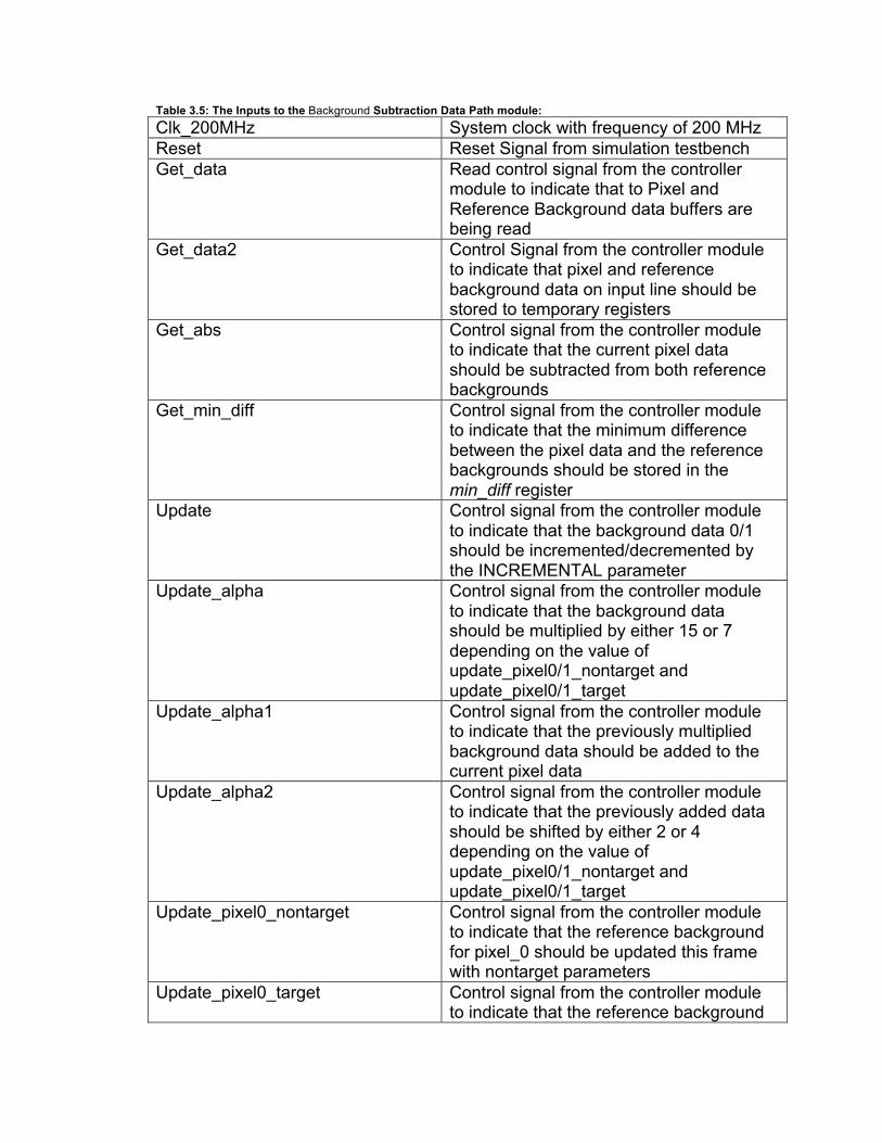
Table 3.5: The Inputs to the Background Subtraction Data Path module: Clk_200MHz System clock with frequency of 200 MHz Reset Reset Signal from simulation testbench Get_data Read control signal from the controller
module to indicate that to Pixel and Reference Background data buffers are being read
Get_data2 Control Signal from the controller module to indicate that pixel and reference background data on input line should be stored to temporary registers
Get_abs Control signal from the controller module to indicate that the current pixel data should be subtracted from both reference backgrounds
Get_min_diff Control signal from the controller module to indicate that the minimum difference between the pixel data and the reference backgrounds should be stored in the min_diff register
Update Control signal from the controller module to indicate that the background data 0/1 should be incremented/decremented by the INCREMENTAL parameter
Update_alpha Control signal from the controller module to indicate that the background data should be multiplied by either 15 or 7 depending on the value of update_pixel0/1_nontarget and update_pixel0/1_target
Update_alpha1 Control signal from the controller module to indicate that the previously multiplied background data should be added to the current pixel data
Update_alpha2 Control signal from the controller module to indicate that the previously added data should be shifted by either 2 or 4 depending on the value of update_pixel0/1_nontarget and update_pixel0/1_target
Update_pixel0_nontarget Control signal from the controller module to indicate that the reference background for pixel_0 should be updated this frame with nontarget parameters
Update_pixel0_target Control signal from the controller module to indicate that the reference background
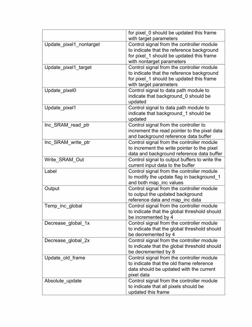
for pixel_0 should be updated this frame with target parameters
Update_pixel1_nontarget Control signal from the controller module to indicate that the reference background for pixel_1 should be updated this frame with nontarget parameters
Update_pixel1_target Control signal from the controller module to indicate that the reference background for pixel_1 should be updated this frame with target parameters
Update_pixel0 Control signal to data path module to indicate that background_0 should be updated
Update_pixel1 Control signal to data path module to indicate that background_1 should be updated
Inc_SRAM_read_ptr Control signal from the controller to increment the read pointer to the pixel data and background reference data buffer
Inc_SRAM_write_ptr Control signal from the controller module to increment the write pointer to the pixel data and background reference data buffer
Write_SRAM_Out Control signal to output buffers to write the current input data to the buffer
Label Control signal from the controller module to modify the update flag in background_1 and both map_inc values
Output Control signal from the controller module to output the updated background reference data and map_inc data
Temp_inc_global Control signal from the controller module to indicate that the global threshold should be incremented by 4
Decrease_global_1x Control signal from the controller module to indicate that the global threshold should be decremented by 4
Decrease_global_2x Control signal from the controller module to indicate that the global threshold should be decremented by 8
Update_old_frame Control signal from the controller module to indicate that the old frame reference data should be updated with the current pixel data
Absolute_update Control signal from the controller module to indicate that all pixels should be updated this frame
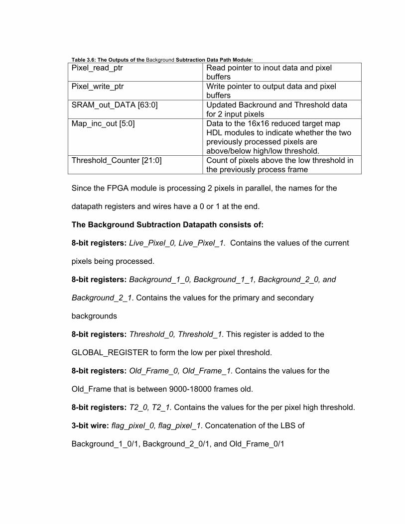
Table 3.6: The Outputs of the Background Subtraction Data Path Module: Pixel_read_ptr Read pointer to inout data and pixel
buffers Pixel_write_ptr Write pointer to output data and pixel
buffers SRAM_out_DATA [63:0] Updated Backround and Threshold data
for 2 input pixels Map_inc_out [5:0] Data to the 16x16 reduced target map
HDL modules to indicate whether the two previously processed pixels are above/below high/low threshold.
Threshold_Counter [21:0] Count of pixels above the low threshold in the previously process frame
Since the FPGA module is processing 2 pixels in parallel, the names for the
datapath registers and wires have a 0 or 1 at the end.
The Background Subtraction Datapath consists of: 8-bit registers: Live_Pixel_0, Live_Pixel_1. Contains the values of the current
pixels being processed.
8-bit registers: Background_1_0, Background_1_1, Background_2_0, and
Background_2_1. Contains the values for the primary and secondary
backgrounds
8-bit registers: Threshold_0, Threshold_1. This register is added to the
GLOBAL_REGISTER to form the low per pixel threshold.
8-bit registers: Old_Frame_0, Old_Frame_1. Contains the values for the
Old_Frame that is between 9000-18000 frames old.
8-bit registers: T2_0, T2_1. Contains the values for the per pixel high threshold.
3-bit wire: flag_pixel_0, flag_pixel_1. Concatenation of the LBS of
Background_1_0/1, Background_2_0/1, and Old_Frame_0/1
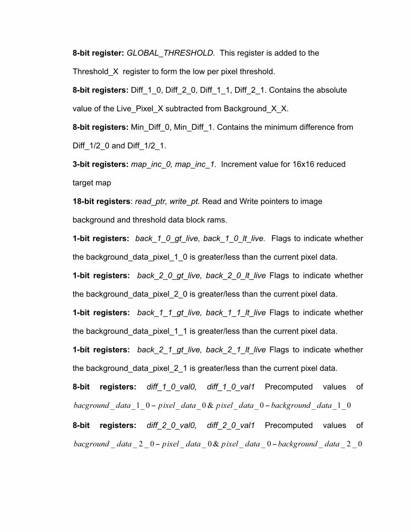
8-bit register: GLOBAL_THRESHOLD. This register is added to the
Threshold_X register to form the low per pixel threshold.
8-bit registers: Diff_1_0, Diff_2_0, Diff_1_1, Diff_2_1. Contains the absolute
value of the Live_Pixel_X subtracted from Background_X_X.
8-bit registers: Min_Diff_0, Min_Diff_1. Contains the minimum difference from
Diff_1/2_0 and Diff_1/2_1.
3-bit registers: map_inc_0, map_inc_1. Increment value for 16x16 reduced
target map
18-bit registers: read_ptr, write_pt. Read and Write pointers to image
background and threshold data block rams.
1-bit registers: back_1_0_gt_live, back_1_0_lt_live. Flags to indicate whether
the background_data_pixel_1_0 is greater/less than the current pixel data.
1-bit registers: back_2_0_gt_live, back_2_0_lt_live Flags to indicate whether
the background_data_pixel_2_0 is greater/less than the current pixel data.
1-bit registers: back_1_1_gt_live, back_1_1_lt_live Flags to indicate whether
the background_data_pixel_1_1 is greater/less than the current pixel data.
1-bit registers: back_2_1_gt_live, back_2_1_lt_live Flags to indicate whether
the background_data_pixel_2_1 is greater/less than the current pixel data.
8-bit registers: diff_1_0_val0, diff_1_0_val1 Precomputed values of
8-bit registers: diff_2_0_val0, diff_2_0_val1 Precomputed values of

8-bit registers: diff_1_1_val0, diff_1_1_val1 Precomputed values of
8-bit registers: diff_2_1_val0, diff_2_1_val1 Precomputed values of
3.3 16x16 Reduced Target Map
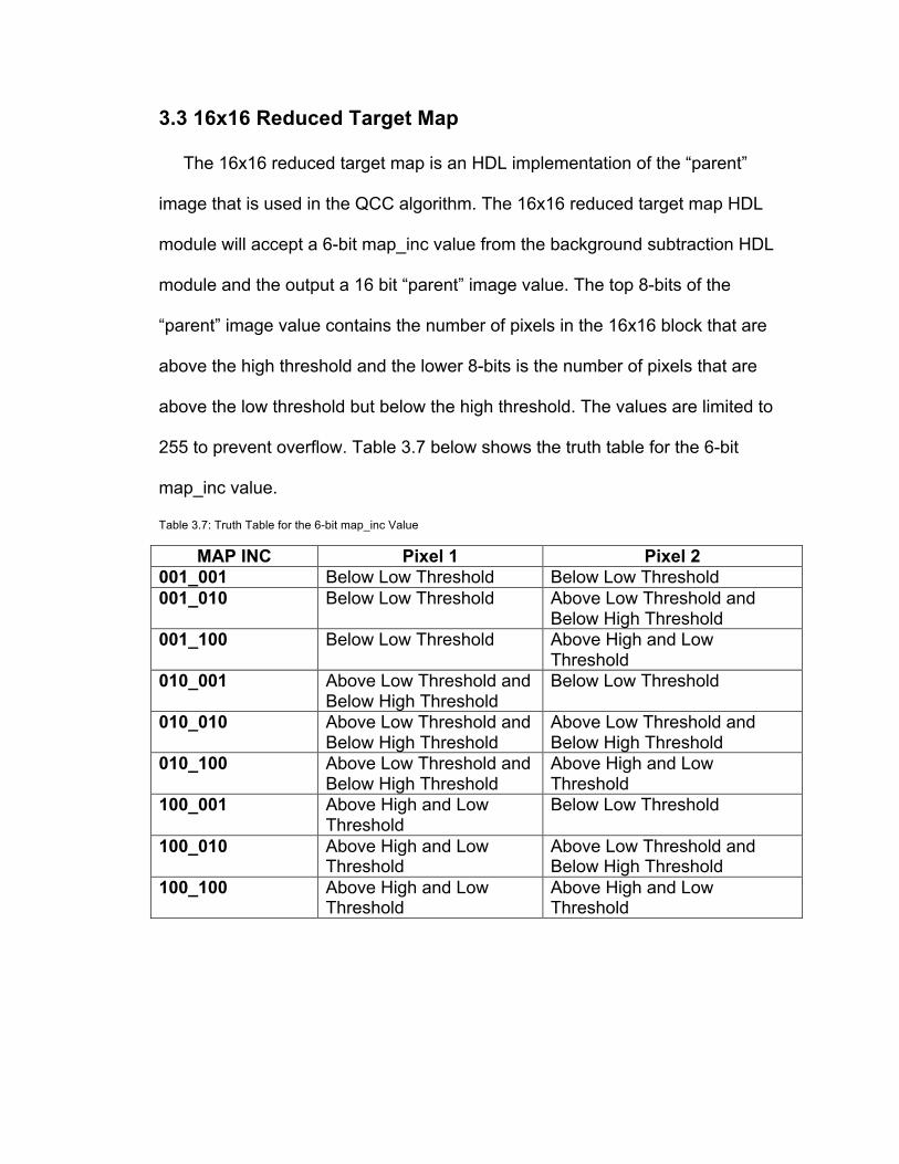
The 16x16 reduced target map is an HDL implementation of the “parent”
image that is used in the QCC algorithm. The 16x16 reduced target map HDL
module will accept a 6-bit map_inc value from the background subtraction HDL
module and the output a 16 bit “parent” image value. The top 8-bits of the
“parent” image value contains the number of pixels in the 16x16 block that are
above the high threshold and the lower 8-bits is the number of pixels that are
above the low threshold but below the high threshold. The values are limited to
255 to prevent overflow. Table 3.7 below shows the truth table for the 6-bit
map_inc value.
Table 3.7: Truth Table for the 6-bit map_inc Value
MAP INC Pixel 1 Pixel 2 001_001 Below Low Threshold Below Low Threshold 001_010 Below Low Threshold Above Low Threshold and
Below High Threshold 001_100 Below Low Threshold Above High and Low
Threshold 010_001 Above Low Threshold and
Below High Threshold Below Low Threshold
010_010 Above Low Threshold and Below High Threshold
Above Low Threshold and Below High Threshold
010_100 Above Low Threshold and Below High Threshold
Above High and Low Threshold
100_001 Above High and Low Threshold
Below Low Threshold
100_010 Above High and Low Threshold
Above Low Threshold and Below High Threshold
100_100 Above High and Low Threshold
Above High and Low Threshold
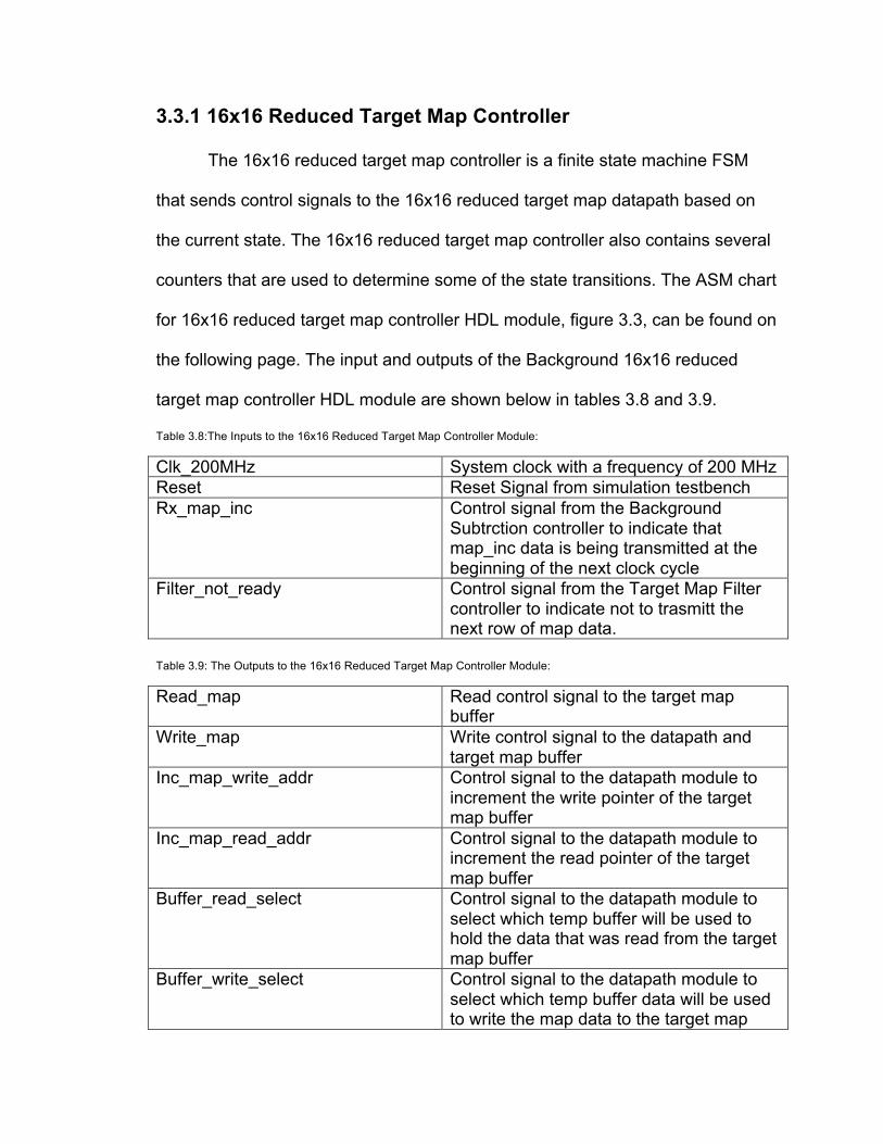
3.3.1 16x16 Reduced Target Map Controller
The 16x16 reduced target map controller is a finite state machine FSM
that sends control signals to the 16x16 reduced target map datapath based on
the current state. The 16x16 reduced target map controller also contains several
counters that are used to determine some of the state transitions. The ASM chart
for 16x16 reduced target map controller HDL module, figure 3.3, can be found on
the following page. The input and outputs of the Background 16x16 reduced
target map controller HDL module are shown below in tables 3.8 and 3.9.
Table 3.8:The Inputs to the 16x16 Reduced Target Map Controller Module:
Clk_200MHz System clock with a frequency of 200 MHz Reset Reset Signal from simulation testbench Rx_map_inc Control signal from the Background
Subtrction controller to indicate that map_inc data is being transmitted at the beginning of the next clock cycle
Filter_not_ready Control signal from the Target Map Filter controller to indicate not to trasmitt the next row of map data.
Table 3.9: The Outputs to the 16x16 Reduced Target Map Controller Module:
Read_map Read control signal to the target map buffer
Write_map Write control signal to the datapath and target map buffer
Inc_map_write_addr Control signal to the datapath module to increment the write pointer of the target map buffer
Inc_map_read_addr Control signal to the datapath module to increment the read pointer of the target map buffer
Buffer_read_select Control signal to the datapath module to select which temp buffer will be used to hold the data that was read from the target map buffer
Buffer_write_select Control signal to the datapath module to select which temp buffer data will be used to write the map data to the target map

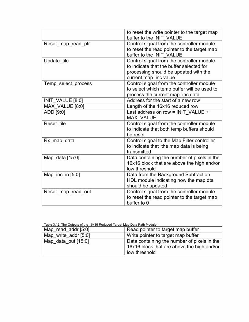
buffer Reset_map Control signal to the datapath module to
indicate that the map buffer is being reset. Reset_map_write_ptr Control signal to the datapath module to
reset the write pointer to the target map buffer to the INIT_VALUE
Reset_map_read_ptr Control signal to the datapath module to reset the read pointer to the target map buffer to the INIT_VALUE
Update_tile Control signal to the datapath module to indicate that the buffer selected for processing should be updated with the current map_inc value
Temp_select_process Control signal to the datapath module to select which temp buffer will be used to process the current map_inc data
INIT_VALUE [8:0] Address for the start of a new row MAX_VALUE [8:0] Length of the 16x16 reduced row ADD [9:0] Last address on row = INIT_VALUE +
MAX_VALUE Reset_tile Control signal to the datapath module to
indicate that both temp buffers should be reset
Rx_map_data Control signal to the Map Filter controller to indicate that the map data is being transmitted
Reset_map_read_out Control signal to the datapath module to reset the read pointer to the target map buffer to 0
Furthermore, the 16x16 reduced target map is fully parameterized to allow for
different block sizes and image sizes.
PARAMETERS for the 16x16 Reduced Target Map Controller Module Are: parameter PIXELS parameter BLOCK_SIZE=16/PIXELS parameter NUMBER_OF_ROWS parameter SIZE_OF_ROW parameter SIZE_OF_ROW_1= SIZE_OF_ROW/BLOCK_SIZE parameter SIZE_OF_ROW_2= SIZE_OF_ROW/(BLOCK_SIZE*PIXELS)
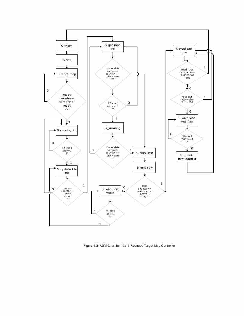
Figure 3.3: ASM Chart for 16x16 Reduced Target Map Controller

Table 3.10 shows the controls signals that are asserted at each state shown in
the asm chart on the previous page. All of the control signals are generated with
combinational logic.
Table 3.10: Control Signals Asserted at Each State 16x16 Reduced Target Map Controller
State Table Control Signals S_reset NONE S_set NONE S_reset_map_init write_map, reset_map, inc_map_write_addr S_running_init S_update_tile_init update_tile, inc_map_read_addr, read_map S_running update_tile, write_map, inc_map_write_addr
S_get_map_inc NONE S_write_last write_map S_new_row reset_map_write_pointer,reset_map_read_pointer S_read_first_value read_map S_wait_read_out_flag NONE S_update_row_counter NONE
Additionally, there are 5 counters that are used to determine some of the state
transitions:
row_update_complete_counter: Used to count the number of rows in the 16x16 reduced image that have been completely updated. update_counter: Used to count the number of updates inside of a 16x16 block. process_counter: Used to count the total number of update reset_counter: Used to count number of blocks that have been reset to 0. read_out_counter: Counts the number of blocks that have been sent to the target map filter HDL module.

3.3.2 16x16 Reduced Target Map Datapath
The 16x16 Reduced Target Map Datapath HDL module will process the
map_inc data from the background subtraction HDL modules and form a 16x16
area count of the number of pixels above the high and low thresholds. Control
signals received from the 16x16 reduced target map controller will signal the
datapath to perform operations such as updating the 16x16 block counter based
on the value of map_inc and reading and writing to the temporary target map
buffers. The input and outputs of the 16x16 Reduced Target Map datapath HDL
module are shown below in tables 3.11 and 3.12
Table 3.11: The Inputs to 16x16 Reduced Target Map Data Path Module:
Clk_200MHz System clock with a frequency of 200 MHz Reset Reset Signal from simulation testbench Rx_map_inc Control signal from the Background
Subtraction controller to indicate that map_inc data is being transmitted
Read_map Read control signal to the target map buffer
Write_map Write control signal to the datapath and target map buffer
Inc_map_write_addr Control signal from the controller module to increment the write pointer to the target map buffer
Inc_map_read_addr Control signal from the controller module to increment the read pointer to the target map buffer
Buffer_read_select Control signal from the controller module to select which temp buffer will be used to hold the data that was read from the target map buffer
Buffer_write_select Control signal from the controller module to select which temp buffer will be used to write the map data to the target map buffer
Reset_map Control signal from the controller module to indicate that the map buffer is being reset.
Reset_map_write_ptr Control signal from the controller module
to reset the write pointer to the target map buffer to the INIT_VALUE
Reset_map_read_ptr Control signal from the controller module to reset the read pointer to the target map buffer to the INIT_VALUE
Update_tile Control signal from the controller module to indicate that the buffer selected for processing should be updated with the current map_inc value
Temp_select_process Control signal from the controller module to select which temp buffer will be used to process the current map_inc data
INIT_VALUE [8:0] Address for the start of a new row MAX_VALUE [8:0] Length of the 16x16 reduced row ADD [9:0] Last address on row = INIT_VALUE +
MAX_VALUE Reset_tile Control signal from the controller module
to indicate that both temp buffers should be reset
Rx_map_data Control signal to the Map Filter controller to indicate that the map data is being transmitted
Map_data [15:0] Data containing the number of pixels in the 16x16 block that are above the high and/or low threshold
Map_inc_in [5:0] Data from the Background Subtraction HDL module indicating how the map dta should be updated
Reset_map_read_out Control signal from the controller module to reset the read pointer to the target map buffer to 0
Table 3.12: The Outputs of the 16x16 Reduced Target Map Data Path Module:
Map_read_addr [5:0] Read pointer to target map buffer Map_write_addr [5:0] Write pointer to target map buffer Map_data_out [15:0] Data containing the number of pixels in the
16x16 block that are above the high and/or low threshold

The 16x16 Reduced Target Map Data Datapath further consists of: 1-bit register: read_map_delay. read map delayed by 1 clock cycle 5-bit registers: map_inc_temp0, map_inc_temp. Temporary buffer to hold current map_inc value 16-bit registers: map_temp0, map_temp1. Temporary buffer to hold the current map data. 3.4 TARGET MAP FILTER HDL Module
The target map filter HDL module will parse every row of the 16x16 reduced
“parent” image from the 16x16 reduced target map HDL module output buffer.
On every row of the “parent” image the target map filter will insert two 16-bit
values. The first value is the position of the left most pixel that is above threshold.
The second value is the position of the right most pixel above threshold. These
inserted values will allow the connected components algorithm execute faster
since it will only have to process parts of the row that contains pixels that are
above threshold. After a row is processed by the target map filter modules, the
data will be written to a PowerPC accessible block ram for connected compinents
processing.
3.4.1 TARGET MAP FILTER Controller
The target map filter controller is a finite state machine FSM that sends
control signals to the target map filter datapath based on the current state. The
target map filter controller also contains counters that are used to determine
some of the state transitions. The ASM chart for the target map filter controller
HDL module, figure 3.4, can be found on the following page. The input and
outputs of the target map filter controller HDL module are shown below in tables
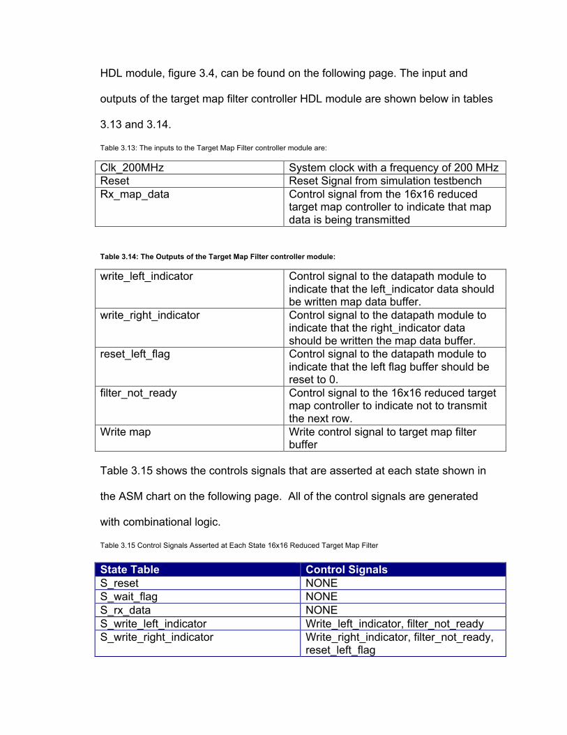
3.13 and 3.14.
Table 3.13: The inputs to the Target Map Filter controller module are:
Clk_200MHz System clock with a frequency of 200 MHz Reset Reset Signal from simulation testbench Rx_map_data Control signal from the 16x16 reduced
target map controller to indicate that map data is being transmitted
Table 3.14: The Outputs of the Target Map Filter controller module:
write_left_indicator Control signal to the datapath module to indicate that the left_indicator data should be written map data buffer.
write_right_indicator Control signal to the datapath module to indicate that the right_indicator data should be written the map data buffer.
reset_left_flag Control signal to the datapath module to indicate that the left flag buffer should be reset to 0.
filter_not_ready Control signal to the 16x16 reduced target map controller to indicate not to transmit the next row.
Write map Write control signal to target map filter buffer
Table 3.15 shows the controls signals that are asserted at each state shown in
the ASM chart on the following page. All of the control signals are generated
with combinational logic.
Table 3.15 Control Signals Asserted at Each State 16x16 Reduced Target Map Filter
State Table Control Signals S_reset NONE S_wait_flag NONE S_rx_data NONE S_write_left_indicator Write_left_indicator, filter_not_ready S_write_right_indicator Write_right_indicator, filter_not_ready,
reset_left_flag

Figure 3.4: ASM Chart for Target Map Filter Controller
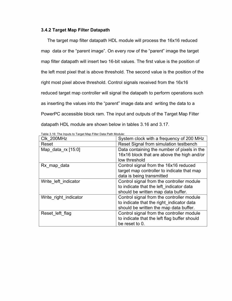
3.4.2 Target Map Filter Datapath
The target map filter datapath HDL module will process the 16x16 reduced
map data or the “parent image”. On every row of the “parent” image the target
map filter datapath will insert two 16-bit values. The first value is the position of
the left most pixel that is above threshold. The second value is the position of the
right most pixel above threshold. Control signals received from the 16x16
reduced target map controller will signal the datapath to perform operations such
as inserting the values into the “parent” image data and writing the data to a
PowerPC accessible block ram. The input and outputs of the Target Map Filter
datapath HDL module are shown below in tables 3.16 and 3.17.
Table 3.16: The Inputs to Target Map Filter Data Path Module:
Clk_200MHz System clock with a frequency of 200 MHz Reset Reset Signal from simulation testbench Map_data_rx [15:0] Data containing the number of pixels in the
16x16 block that are above the high and/or low threshold
Rx_map_data Control signal from the 16x16 reduced target map controller to indicate that map data is being transmitted
Write_left_indicator Control signal from the controller module to indicate that the left_indicator data should be written map data buffer.
Write_right_indicator Control signal from the controller module to indicate that the right_indicator data should be written the map data buffer.
Reset_left_flag Control signal from the controller module to indicate that the left flag buffer should be reset to 0.

Table 3.17 :The Outputs of the Target Map Filter Data Path Module:
Write_ptr [`TARGET_REG_SIZE-1:0] Write pointer to the target map filter buffer
Map_data_out [15:0] Data containing the number of pixels in the 16x16 block that are above the high and/or low threshold, tags on each row
Additional registers of the Target Map Filter Datapath are: 1-bit register: rx_map_delay. rx_map signal delayed by 1 clock cycle 1-bit register: left_flag. Flag to indicate the first pixel that is above threshold on the current row has been located. 16-bit registers: left_indicator_flag, right_indicator_flag. Position of the first and last pixel on the row that is above threshold.
CHAPTER 4
SIMULATION/SYNTHESIS RESULTS
CHAPTER 4
SIMULATION/SYNTHESIS RESULTS
4.1 Simulation Introduction
This chapter contains simulation results for the background subtraction, 16x16
reduced target map, and target filter HDL modules. The full version of the
simulator built into Xilinx ISE was used to simulate all of the Verilog HDL
modules. Additionally, file I/O commands added in the Verilog 2001 standard
were used to load the image, background reference and threshold data to
multiple block ram modules and write the simulation data from a block ram
module back to an image file. The final simulation of the background subtraction
HDL modules consisted of producing threshold images that shows the pixels that
are above the high and low threshold image for each input image, a count of the
pixels above threshold for each input image, and the 6-bit map_inc value. The
high and low output threshold images were produced according to equations 4.1
and 4.2:
The 16x6 reduced target map filter was simulated using both a constant map_inc
value and the actual map_inc values for each of the input images generated from
the background subtraction HDL modules. Finally, the target map filter HDL
module was simulated using the 16-bit map value from the 16x16 reduced target
map output buffer data.
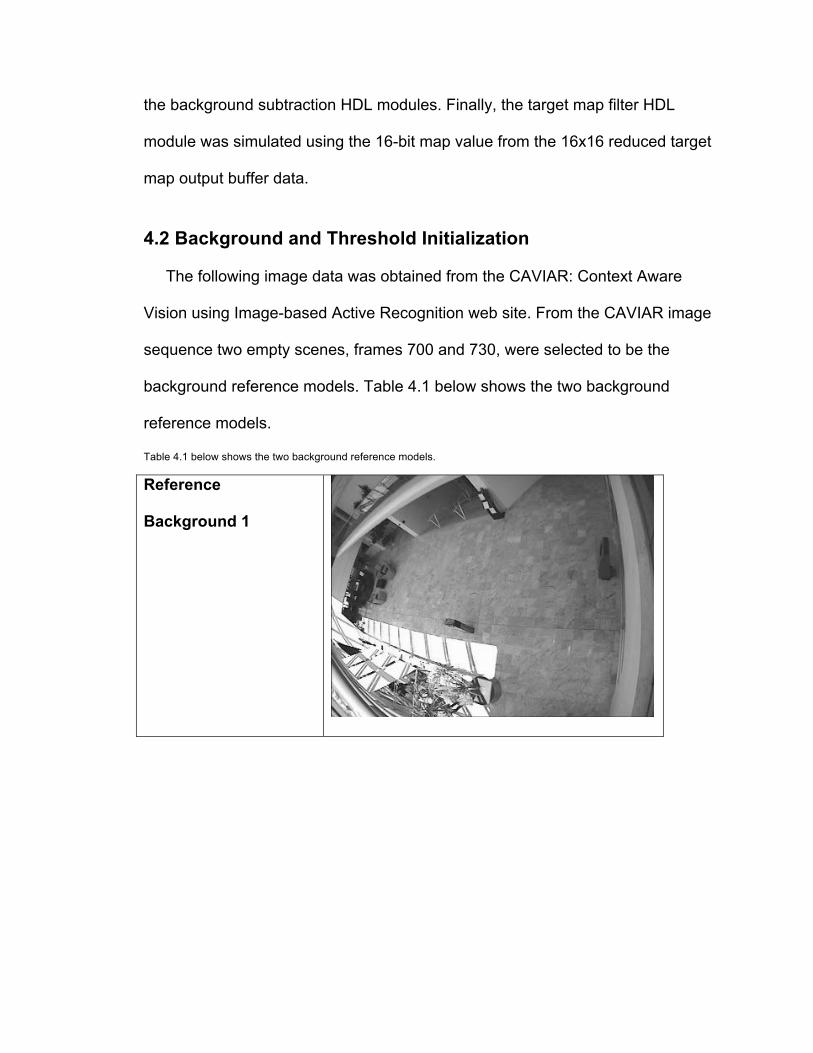
4.2 Background and Threshold Initialization The following image data was obtained from the CAVIAR: Context Aware
Vision using Image-based Active Recognition web site. From the CAVIAR image
sequence two empty scenes, frames 700 and 730, were selected to be the
background reference models. Table 4.1 below shows the two background
reference models.
Table 4.1 below shows the two background reference models.
Reference
Background 1
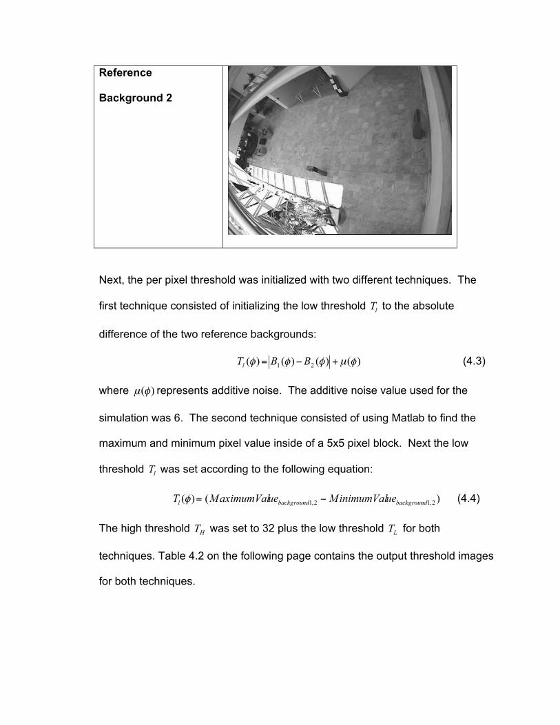
Reference
Background 2
Next, the per pixel threshold was initialized with two different techniques. The
first technique consisted of initializing the low threshold to the absolute
difference of the two reference backgrounds:
(4.3)
where represents additive noise. The additive noise value used for the
simulation was 6. The second technique consisted of using Matlab to find the
maximum and minimum pixel value inside of a 5x5 pixel block. Next the low
threshold was set according to the following equation:
(4.4)
The high threshold was set to 32 plus the low threshold for both
techniques. Table 4.2 on the following page contains the output threshold images
for both techniques.

Table 4.2 on the following page contains the output threshold images for both techniques
Threshold image using
technique # 1
Threshold image using
technique # 2

4.3 Simulation Results for the Background Subtraction HDL Modules
4.3.1 Experiments with FRAME 870
Table 4.3 below shows the Verilog HDL simulation results for Caviar Frame
870.The first set of threshold images were produced using the absolute value
plus additive noise threshold initialization technique and the second set of
images was produced using the 5x5 block average threshold initialization
technique. Table 4.3 also contains the count of the number of pixels above
threshold for both techniques. The scene contains three targets that are show
inside of the red boxes.
Table 4.3: Verilog HDL Simulation Results for Caviar Frame 870
Frame 870

Pixels above the low threshold using threshold initialization technique #1
Pixels above the low threshold using threshold initialization technique #2

Pixels above the high threshold using threshold initialization technique #1
Pixels above the high threshold using threshold initialization technique #2
Pixels above threshold
Threshold Initialization Technique #1: 2421 pixels #2: 521 pixels

4.3.2 Experiments with FRAME 911
Table 4.4 below shows the Verilog HDL simulation results for Caviar Frame
911.The first set of threshold images were produced using the absolute value
plus additive noise threshold initialization technique and the second set of
images was produced using the 5x5 block average threshold initialization
technique. Table 4.4 also contains the count of the number of pixels above
threshold for both techniques. The scene contains three targets that are show
inside of the red boxes.
Table 4.4: Verilog HDL Simulation Results for Caviar Frame 911
FRAME 911
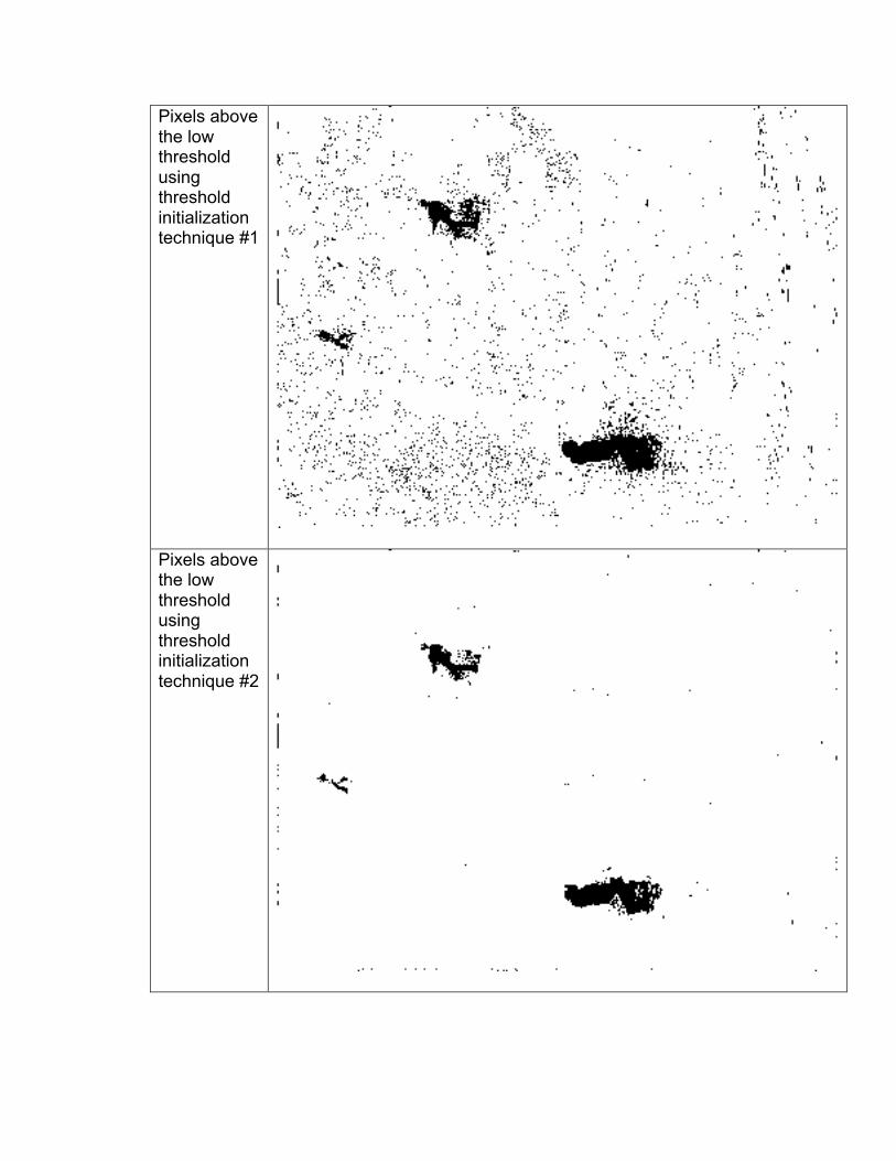
Pixels above the low threshold using threshold initialization technique #1
Pixels above the low threshold using threshold initialization technique #2
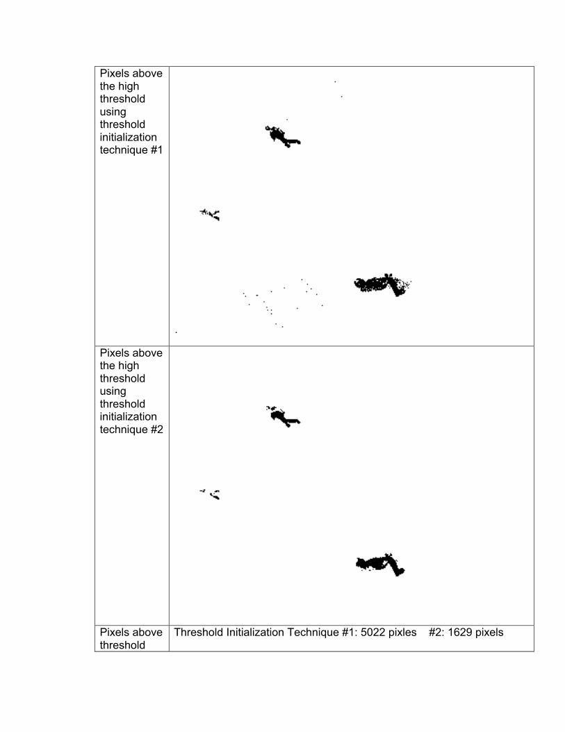
Pixels above the high threshold using threshold initialization technique #1
Pixels above the high threshold using threshold initialization technique #2
Pixels above threshold
Threshold Initialization Technique #1: 5022 pixles #2: 1629 pixels
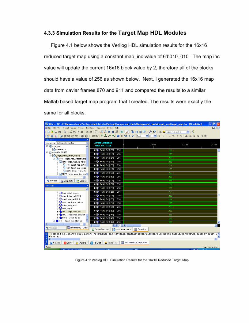
4.3.3 Simulation Results for the Target Map HDL Modules
Figure 4.1 below shows the Verilog HDL simulation results for the 16x16
reduced target map using a constant map_inc value of 6’b010_010. The map inc
value will update the current 16x16 block value by 2, therefore all of the blocks
should have a value of 256 as shown below. Next, I generated the 16x16 map
data from caviar frames 870 and 911 and compared the results to a similar
Matlab based target map program that I created. The results were exactly the
same for all blocks.
Figure 4.1: Verilog HDL Simulation Results for the 16x16 Reduced Target Map
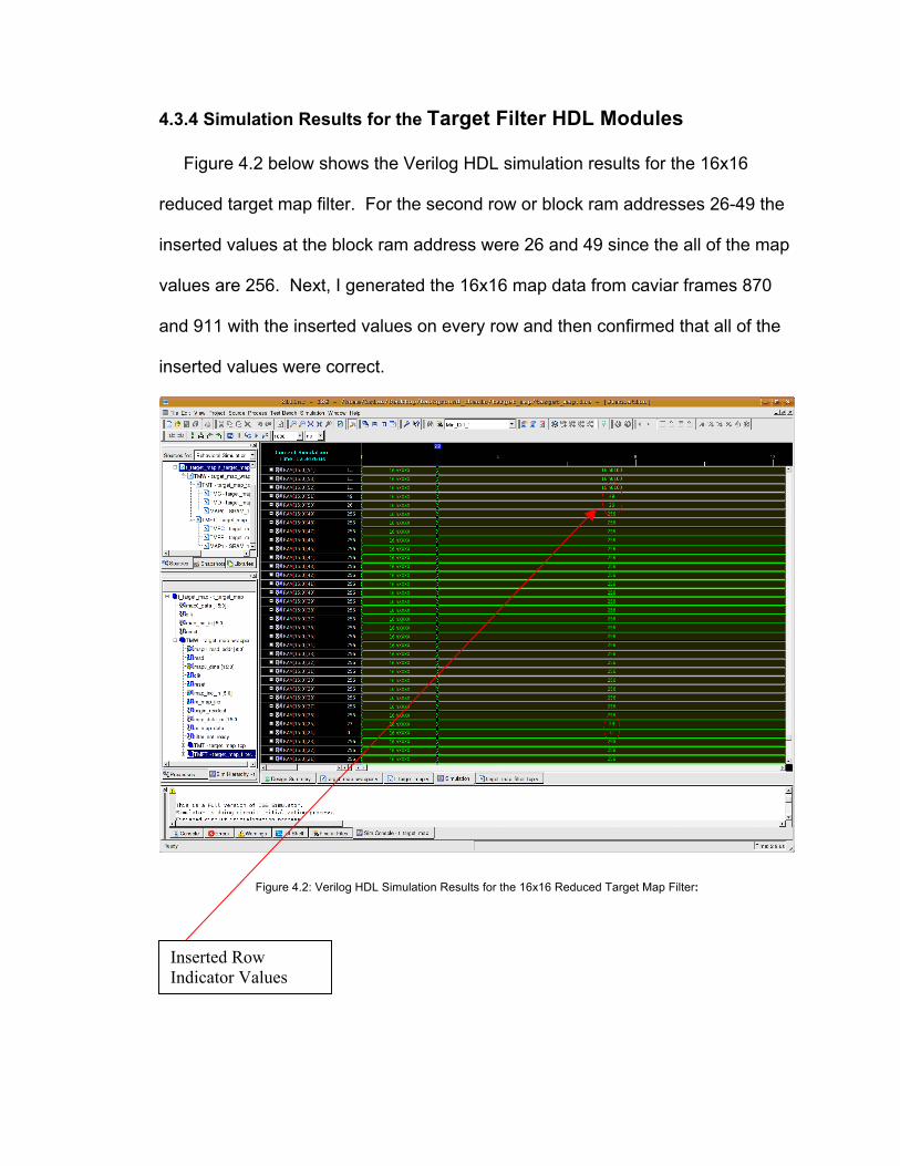
4.3.4 Simulation Results for the Target Filter HDL Modules
Figure 4.2 below shows the Verilog HDL simulation results for the 16x16
reduced target map filter. For the second row or block ram addresses 26-49 the
inserted values at the block ram address were 26 and 49 since the all of the map
values are 256. Next, I generated the 16x16 map data from caviar frames 870
and 911 with the inserted values on every row and then confirmed that all of the
inserted values were correct.
Figure 4.2: Verilog HDL Simulation Results for the 16x16 Reduced Target Map Filter:
Inserted Row Indicator Values
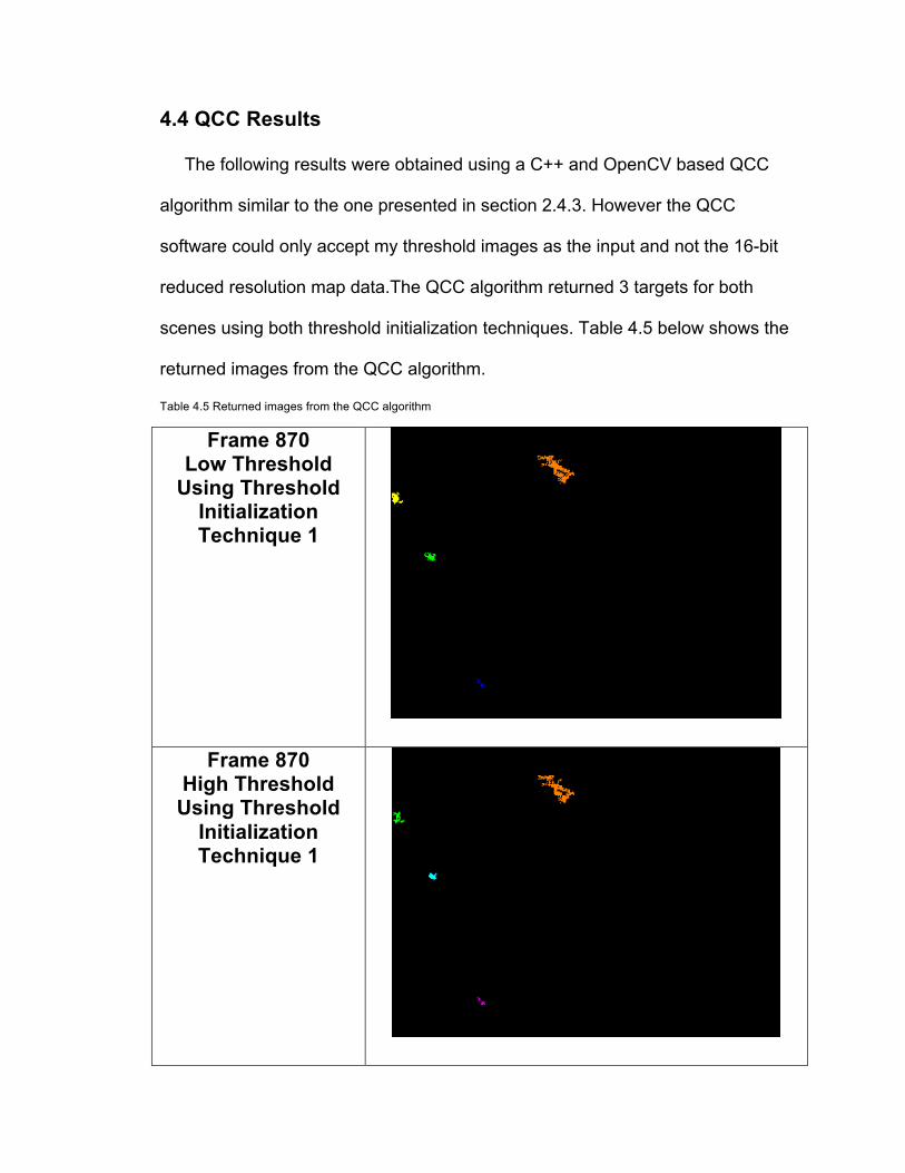
4.4 QCC Results
The following results were obtained using a C++ and OpenCV based QCC
algorithm similar to the one presented in section 2.4.3. However the QCC
software could only accept my threshold images as the input and not the 16-bit
reduced resolution map data.The QCC algorithm returned 3 targets for both
scenes using both threshold initialization techniques. Table 4.5 below shows the
returned images from the QCC algorithm.
Table 4.5 Returned images from the QCC algorithm
Frame 870 Low Threshold
Using Threshold Initialization Technique 1
Frame 870 High Threshold
Using Threshold Initialization Technique 1
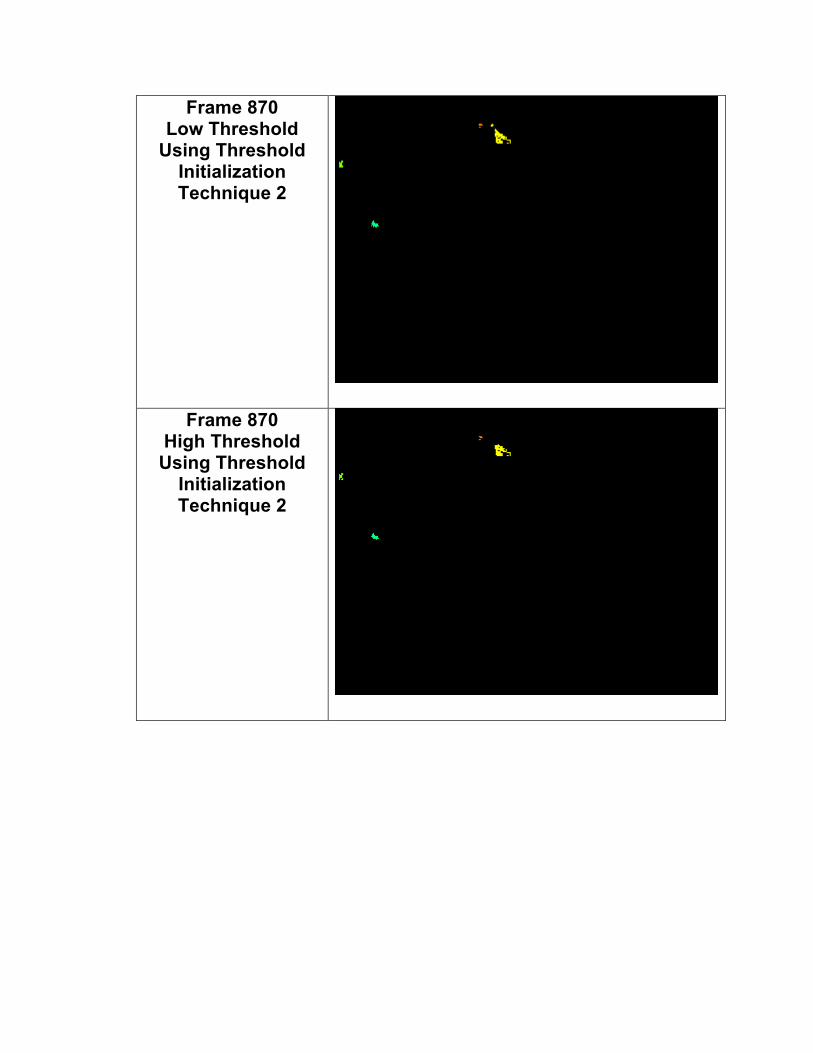
Frame 870 Low Threshold
Using Threshold Initialization Technique 2
Frame 870 High Threshold
Using Threshold Initialization Technique 2

Frame 911 Low Threshold
Using Threshold Initialization Technique 1
Frame 911 High Threshold
Using Threshold Initialization Technique 1
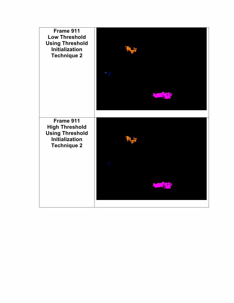
Frame 911 Low Threshold
Using Threshold Initialization Technique 2
Frame 911 High Threshold
Using Threshold Initialization Technique 2
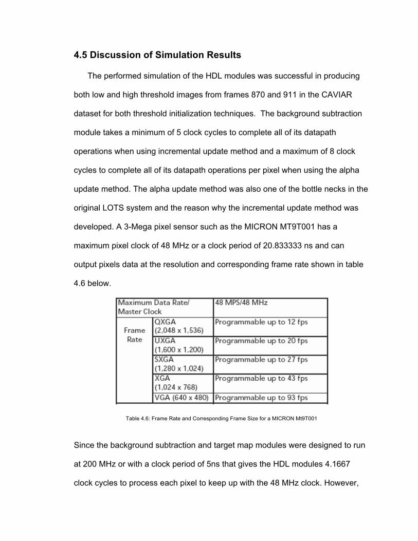
4.5 Discussion of Simulation Results
The performed simulation of the HDL modules was successful in producing
both low and high threshold images from frames 870 and 911 in the CAVIAR
dataset for both threshold initialization techniques. The background subtraction
module takes a minimum of 5 clock cycles to complete all of its datapath
operations when using incremental update method and a maximum of 8 clock
cycles to complete all of its datapath operations per pixel when using the alpha
update method. The alpha update method was also one of the bottle necks in the
original LOTS system and the reason why the incremental update method was
developed. A 3-Mega pixel sensor such as the MICRON MT9T001 has a
maximum pixel clock of 48 MHz or a clock period of 20.833333 ns and can
output pixels data at the resolution and corresponding frame rate shown in table
4.6 below.
Table 4.6: Frame Rate and Corresponding Frame Size for a MICRON Mt9T001
Since the background subtraction and target map modules were designed to run
at 200 MHz or with a clock period of 5ns that gives the HDL modules 4.1667
clock cycles to process each pixel to keep up with the 48 MHz clock. However,
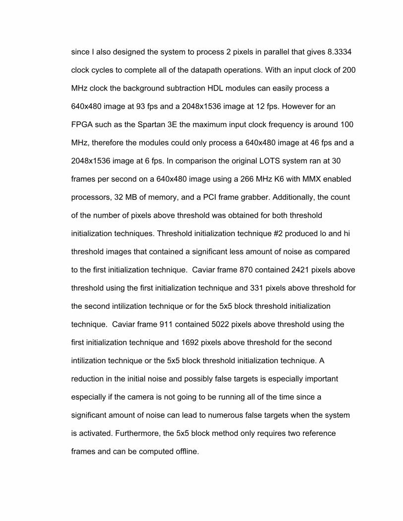
since I also designed the system to process 2 pixels in parallel that gives 8.3334
clock cycles to complete all of the datapath operations. With an input clock of 200
MHz clock the background subtraction HDL modules can easily process a
640x480 image at 93 fps and a 2048x1536 image at 12 fps. However for an
FPGA such as the Spartan 3E the maximum input clock frequency is around 100
MHz, therefore the modules could only process a 640x480 image at 46 fps and a
2048x1536 image at 6 fps. In comparison the original LOTS system ran at 30
frames per second on a 640x480 image using a 266 MHz K6 with MMX enabled
processors, 32 MB of memory, and a PCI frame grabber. Additionally, the count
of the number of pixels above threshold was obtained for both threshold
initialization techniques. Threshold initialization technique #2 produced lo and hi
threshold images that contained a significant less amount of noise as compared
to the first initialization technique. Caviar frame 870 contained 2421 pixels above
threshold using the first initialization technique and 331 pixels above threshold for
the second intilization technique or for the 5x5 block threshold initialization
technique. Caviar frame 911 contained 5022 pixels above threshold using the
first initialization technique and 1692 pixels above threshold for the second
intilization technique or the 5x5 block threshold initialization technique. A
reduction in the initial noise and possibly false targets is especially important
especially if the camera is not going to be running all of the time since a
significant amount of noise can lead to numerous false targets when the system
is activated. Furthermore, the 5x5 block method only requires two reference
frames and can be computed offline.
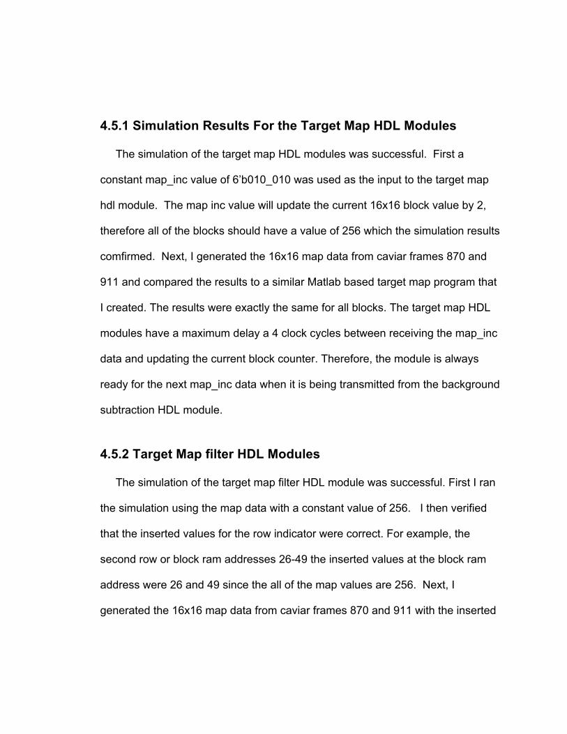
4.5.1 Simulation Results For the Target Map HDL Modules
The simulation of the target map HDL modules was successful. First a
constant map_inc value of 6’b010_010 was used as the input to the target map
hdl module. The map inc value will update the current 16x16 block value by 2,
therefore all of the blocks should have a value of 256 which the simulation results
comfirmed. Next, I generated the 16x16 map data from caviar frames 870 and
911 and compared the results to a similar Matlab based target map program that
I created. The results were exactly the same for all blocks. The target map HDL
modules have a maximum delay a 4 clock cycles between receiving the map_inc
data and updating the current block counter. Therefore, the module is always
ready for the next map_inc data when it is being transmitted from the background
subtraction HDL module.
4.5.2 Target Map filter HDL Modules
The simulation of the target map filter HDL module was successful. First I ran
the simulation using the map data with a constant value of 256. I then verified
that the inserted values for the row indicator were correct. For example, the
second row or block ram addresses 26-49 the inserted values at the block ram
address were 26 and 49 since the all of the map values are 256. Next, I
generated the 16x16 map data from caviar frames 870 and 911 with the inserted
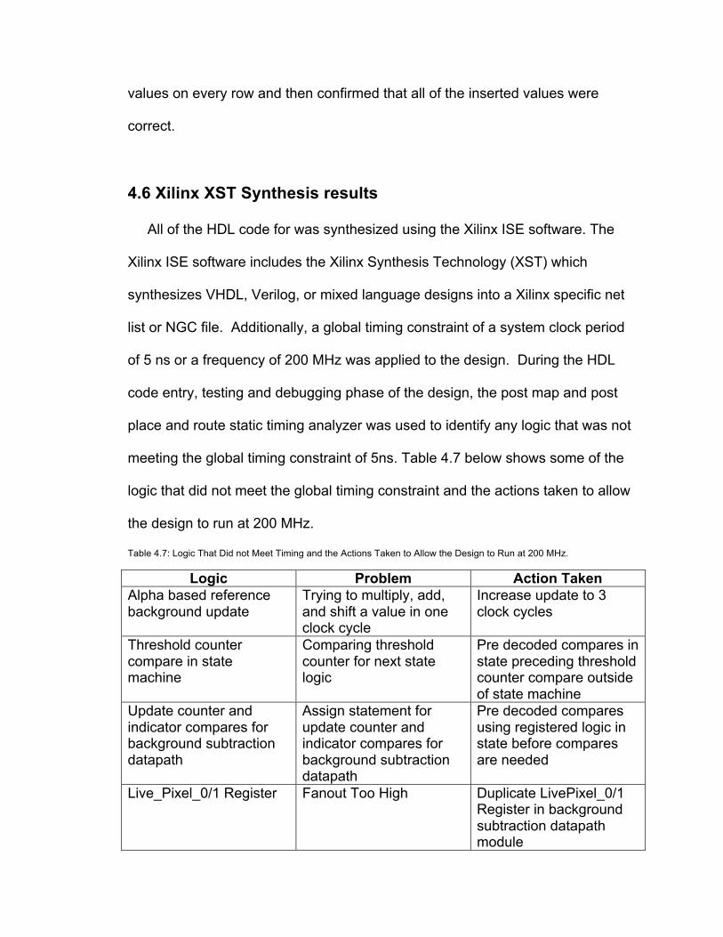
values on every row and then confirmed that all of the inserted values were
correct.
4.6 Xilinx XST Synthesis results
All of the HDL code for was synthesized using the Xilinx ISE software. The
Xilinx ISE software includes the Xilinx Synthesis Technology (XST) which
synthesizes VHDL, Verilog, or mixed language designs into a Xilinx specific net
list or NGC file. Additionally, a global timing constraint of a system clock period
of 5 ns or a frequency of 200 MHz was applied to the design. During the HDL
code entry, testing and debugging phase of the design, the post map and post
place and route static timing analyzer was used to identify any logic that was not
meeting the global timing constraint of 5ns. Table 4.7 below shows some of the
logic that did not meet the global timing constraint and the actions taken to allow
the design to run at 200 MHz.
Table 4.7: Logic That Did not Meet Timing and the Actions Taken to Allow the Design to Run at 200 MHz.
Logic Problem Action Taken Alpha based reference background update
Trying to multiply, add, and shift a value in one clock cycle
Increase update to 3 clock cycles
Threshold counter compare in state machine
Comparing threshold counter for next state logic
Pre decoded compares in state preceding threshold counter compare outside of state machine
Update counter and indicator compares for background subtraction datapath
Assign statement for update counter and indicator compares for background subtraction datapath
Pre decoded compares using registered logic in state before compares are needed
Live_Pixel_0/1 Register Fanout Too High Duplicate LivePixel_0/1 Register in background subtraction datapath module
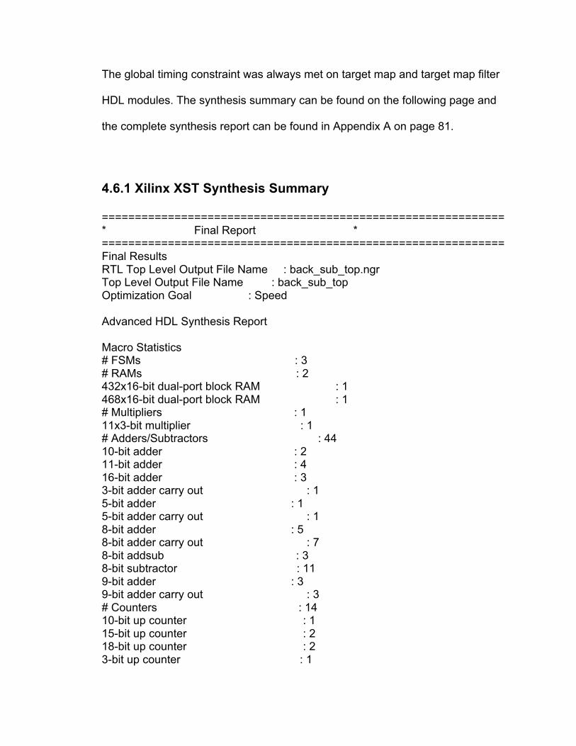
The global timing constraint was always met on target map and target map filter
HDL modules. The synthesis summary can be found on the following page and
the complete synthesis report can be found in Appendix A on page 81.
4.6.1 Xilinx XST Synthesis Summary
============================================================= * Final Report * ============================================================= Final Results RTL Top Level Output File Name : back_sub_top.ngr Top Level Output File Name : back_sub_top Optimization Goal : Speed Advanced HDL Synthesis Report Macro Statistics # FSMs : 3 # RAMs : 2 432x16-bit dual-port block RAM : 1 468x16-bit dual-port block RAM : 1 # Multipliers : 1 11x3-bit multiplier : 1 # Adders/Subtractors : 44 10-bit adder : 2 11-bit adder : 4 16-bit adder : 3 3-bit adder carry out : 1 5-bit adder : 1 5-bit adder carry out : 1 8-bit adder : 5 8-bit adder carry out : 7 8-bit addsub : 3 8-bit subtractor : 11 9-bit adder : 3 9-bit adder carry out : 3 # Counters : 14 10-bit up counter : 1 15-bit up counter : 2 18-bit up counter : 2 3-bit up counter : 1

4-bit up counter : 1 5-bit up counter : 1 8-bit up counter : 2 9-bit up counter : 4 # Accumulators : 5 10-bit up accumulator : 1 3-bit up accumulator : 1 5-bit up accumulator : 1 8-bit up accumulator : 1 9-bit up accumulator : 1 # Registers : 379 Flip-Flops : 379 # Comparators : 28 10-bit comparator equal : 1 10-bit comparator lessequal : 1 16-bit comparator lessequal : 2 3-bit comparator not equal : 1 4-bit comparator not equal : 1 5-bit comparator equal : 1 6-bit comparator not equal : 1 8-bit comparator greater : 10 8-bit comparator less : 3 8-bit comparator lessequal : 4 8-bit comparator not equal : 1 9-bit comparator equal : 1 9-bit comparator not equal : 1 Device utilization summary: --------------------------- Selected Device : 4vfx60ff1152-10 xc3s1200eft256-4 Number of Slices: 618 2% 7% Number of Slice Flip Flops: 450 0% 2% Number of 4 input LUTs: 1171 2% 6% Number of FIFO16/RAMB16s: 2 0% 7% Number of GCLKs: 1 3% 4%

Conclusion
In conclusion the design and simulation of the target detection and tracking HDL
modules was a success. The background subtraction datapath while processing
two pixels in parallel is able to complete all of its operations in 5 to 8 clock cycles.
Additionally, the 16x16 reduced target map and target map filter can complete
their datapath operations 4 and 2 clock cycles respectively. Xilinx post place and
route timing reports shows that the design can operate using a input clock of 200
MHz. The design could also be expanded to process 4 pixels in parallel to
accommodate a 5MPixel sensor with a master clock of 96MHz. Two pixel
threshold initialization techniques were also explored. The first technique
consisted of initializing the low threshold to the absolute difference of the two
reference backgrounds:
The second technique consisted of using Matlab to find the maximum and
minimum pixel value inside of a 5x5 pixel block. Next the low threshold was
set according to the following equation:
The second initialization technique produced threshold images that contained a
significantly less amount of noise. A reduction in the initial noise and possibly
false targets is especially important especially if the camera is not going to be
running all of the time since a significant amount of noise can lead to numerous
false targets when the system is activated. Furthermore, the 5x5 block method
only requires two reference frames and can be computed offline.
Xilinx synthesis report showed that the design utilizes approximately 617 FPGA
Slices or 2% of a Virtex 4 FX60 chip. The largest FPGA resource utilization will
come from the use of dual port block rams for the input and output buffers and
16x16 reduced target map buffers. However the buffers can always be scaled
down to make more block ram available to other parts of the system.
Finally, the hardware aspect of the target detection and tracking system is ready
for a real time implementation. However, the QCC software that can use 16x16
reduced resolution map data needs to be developed and implemented. Once the
software has been developed, the complete system can be integrated onto a
FPGA development board for further analysis and real time testing.

Bibliography
[1] T.E. Boult, R.J. Michaels, X. Gao, and M. Eckman. Into the woods: Visual surveillance of noncooperative and camouflaged targets in complex outdoor settings. Proceedings of the IEEE, 89(10):1382-1402, October 2001
[2] I. Haritaoglu, D. Harwood, and L. S. Davis. W4: real-time
surveillance of people and their activities. IEEE Transactions on Pattern Analysis and Machine Intelligence, 22(8):809– 830, August 2000.
[3] I. Haritaoglu, D. Harwood, and L. S. “W4: Who? When? Where? What” [Online document]. Available HTTP: http://www.umiacs.umd.edu/~hismail/W4_outline.htm
[4] C. Wren, A. Azarbayejani, T. Darrell, and A. Pentland. Pfinder: Real-time tracking of the human body. IEEE Transactions on Pattern Analysis and Machine Intelligence, 19(7):780–785, July 1997.
[5] C. Wren, A. Azarbayejani, T. Darrell, and A. “Real-Time Tracking of the Human Body” [Online document]. Available HTTP: http://vismod.media.mit.edu/vismod/demos/pfinder/
[6] Hall, D. Nascimento, J. Ribeiro, P. Andrade, E. Moreno, P. Pesnel, S. List, T. Emonet, R. Fisher, R.B. Victor, J.S. Crowley, J.L. Comparison of target detection algorithms using adaptive background models. Second IEEE Workshop on Visual Surveillance and Performance Evaluation of Tracking and Surveillance, 113-120, October 2005
[7] T.E. Boult, R.J. Michaels, X. Gao, P. Lewis, C. Powers, W. Yin, and A. Erkan.
Frame-Rate Omnidirectional Surveillance and Tracking of Camouflaged and Occuluded Targets. Second IEEE International Workshop on Visual Surveillance, pp48-55, 1999.
[8] T.E. Boult, R.J. Michaels, X. Gao, P. Lewis, C. Powers, W. Yin, C. Qian, and
A. Erkan. Frame-Rate Multi-Body Tracking for Surveillance. In Proc. of the DARPA IUP. 1998