arX

iv:c

ond-

mat

/000

2174

v1

11

Feb

2000

Foundations of Dissipative Particle Dynamics

Eirik G. Flekkøy1, Peter V. Coveney2 and Gianni De Fabritiis21Department of Physics, University of Oslo

P.O. Box 1048 Blindern, 0316 Oslo 3, Norway2Centre for Computational Science, Queen Mary and Westfield College,

University of London, London E1 4NS, United Kingdom(August 14, 2002)

We derive a mesoscopic modeling and simulation technique that is very close to the techniqueknown as dissipative particle dynamics. The model is derived from molecular dynamics by meansof a systematic coarse-graining procedure. This procedure links the forces between the dissipativeparticles to a hydrodynamic description of the underlying molecular dynamics (MD) particles. Inparticular, the dissipative particle forces are given directly in terms of the viscosity emergent fromMD, while the interparticle energy transfer is similarly given by the heat conductivity derived fromMD. In linking the microscopic and mesoscopic descriptions we thus rely on the macroscopic de-scription emergent from MD. Thus the rules governing our new form of dissipative particle dynamicsreflect the underlying molecular dynamics; in particular all the underlying conservation laws carryover from the microscopic to the mesoscopic descriptions. We obtain the forces experienced bythe dissipative particles together with an approximate form of the associated equilibrium distribu-tion. Whereas previously the dissipative particles were spheres of fixed size and mass, now theyare defined as cells on a Voronoi lattice with variable masses and sizes. This Voronoi lattice arisesnaturally from the coarse-graining procedure which may be applied iteratively and thus representsa form of renormalisation-group mapping. It enables us to select any desired local scale for themesoscopic description of a given problem. Indeed, the method may be used to deal with situationsin which several different length scales are simultaneously present. We compare and contrast thisnew particulate model with existing continuum fluid dynamics techniques, which rely on a purelymacroscopic and phenomenological approach. Simulations carried out with the present scheme showgood agreement with theoretical predictions for the equilibrium behavior.

Pacs numbers: 47.11.+j 47.10.+g 05.40.+j

I. INTRODUCTION

The non-equilibrium behavior of fluids continues topresent a major challenge for both theory and numeri-cal simulation. In recent times, there has been growinginterest in the study of so-called ‘mesoscale’ modelingand simulation methods, particularly for the descriptionof the complex dynamical behavior of many kinds of softcondensed matter, whose properties have thwarted moreconventional approaches. As an example, consider thecase of complex fluids with many coexisting length andtime scales, for which hydrodynamic descriptions are un-known and may not even exist. These kinds of fluids in-clude multi-phase flows, particulate and colloidal suspen-sions, polymers, and amphiphilic fluids, including emul-sions and microemulsions. Fluctuations and Brownianmotion are often key features controlling their behavior.

From the standpoint of traditional fluid dynamics, ageneral problem in describing such fluids is the lack ofadequate continuum models. Such descriptions, whichare usually based on simple conservation laws, approachthe physical description from the macroscopic side, thatis in a ‘top down’ manner, and have certainly provedsuccessful for simple Newtonian fluids [1]. For complexfluids, however, equivalent phenomenological representa-

tions are usually unavailable and instead it is necessaryto base the modeling approach on a microscopic (that ison a particulate) description of the system, thus work-ing from the bottom upwards, along the general lines ofthe program for statistical mechanics pioneered by Boltz-mann [2]. Molecular dynamics (MD) presents itself as themost accurate and fundamental method [3] but it is fartoo computationally intensive to provide a practical op-tion for most hydrodynamic problems involving complexfluids. Over the last decade several alternative ‘bottomup’ strategies have therefore been introduced. Hydrody-namic lattice gases [4], which model the fluid as a discreteset of particles, represent a computationally efficient spa-tial and temporal discretization of the more conventionalmolecular dynamics. The lattice-Boltzmann method [5],originally derived from the lattice-gas paradigm by in-voking Boltzmann’s Stosszahlansatz, represents an inter-mediate (fluctuationless) approach between the top-down(continuum) and bottom-up (particulate) strategies, in-sofar as the basic entity in such models is a single particledistribution function; but for interacting systems eventhese lattice-Boltzmann methods can be subdivided intobottom-up [6] and top-down models [7].

A recent contribution to the family of bottom-upapproaches is the dissipative particle dynamics (DPD)method introduced by Hoogerbrugge and Koelman in

1

1992 [8]. Although in the original formulation of DPDtime was discrete and space continuous, a more recent re-interpretation asserts that this model is in fact a finite-difference approximation to the ‘true’ DPD, which is de-fined by a set of continuous time Langevin equations withmomentum conservation between the dissipative parti-cles [9]. Successful applications of the technique havebeen made to colloidal suspensions [10], polymer solu-tions [11] and binary immiscible fluids [12]. For specificapplications where comparison is possible, this algorithmis orders of magnitude faster than MD [13]. The basicelements of the DPD scheme are particles that representrather ill-defined ‘mesoscopic’ quantities of the underly-ing molecular fluid. These dissipative particles are stipu-lated to evolve in the same way that MD particles do, butwith different inter-particle forces: since the DPD parti-cles are pictured to have internal degrees of freedom, theforces between them have both a fluctuating and a dissi-pative component in addition to the conservative forcesthat are present at the MD level. Newton’s third lawis still satisfied, however, and consequently momentumconservation together with mass conservation producehydrodynamic behavior at the macroscopic level.

Dissipative particle dynamics has been shown to pro-duce the correct macroscopic (continuum) theory; that is,for a one-component DPD fluid, the Navier-Stokes equa-tions emerge in the large scale limit, and the fluid viscos-ity can be computed [14,15]. However, even though dis-sipative particles have generally been viewed as clustersof molecules, no attempt has been made to link DPD tothe underlying microscopic dynamics, and DPD thus re-mains a foundationless algorithm, as is that of the hydro-dynamic lattice gas and a fortiori the lattice-Boltzmannmethod. It is the principal purpose of the present paperto provide an atomistic foundation for dissipative par-ticle dynamics. Among the numerous benefits gainedby achieving this, we are then able to provide a precisedefinition of the term ‘mesoscale’, to relate the hithertopurely phenomenological parameters in the algorithm tounderlying molecular interactions, and thereby to formu-late DPD simulations for specific physicochemical sys-tems, defined in terms of their molecular constituents.The DPD that we derive is a representation of the under-lying MD. Consequently, to the extent that the approxi-mations made are valid, the DPD and MD will have thesame hydrodynamic descriptions, and no separate kinetictheory for, say, the DPD viscosity will be needed once itis known for the MD system. Since the MD degrees offreedom will be integrated out in our approach the MDviscosity will appear in the DPD model as a parameterthat may be tuned freely.

In our approach, the ‘dissipative particles’ (DP) are de-fined in terms of appropriate weight functions that sam-ple portions of the underlying conservative MD parti-cles, and the forces between the dissipative particles areobtained from the hydrodynamic description of the MD

system: the microscopic conservation laws carry over di-rectly to the DPD, and the hydrodynamic behavior ofMD is thus reproduced by the DPD, albeit at a coarserscale. The mesoscopic (coarse-grained) scale of the DPDcan be precisely specified in terms of the MD interac-tions. The size of the dissipative particles, as specifiedby the number of MD particles within them, furnishesthe meaning of the term ‘mesoscopic’ in the present con-text. Since this size is a freely tunable parameter of themodel, the resulting DPD introduces a general proce-dure for simulating microscopic systems at any conve-nient scale of coarse graining, provided that the forcesbetween the dissipative particles are known. When a hy-drodynamic description of the underlying particles canbe found, these forces follow directly; in cases where thisis not possible, the forces between dissipative particlesmust be supplemented with the additional componentsof the physical description that enter on the mesoscopiclevel.

The DPD model which we derive from molecular dy-namics is formally similar to conventional, albeit foun-dationless, DPD [14]. The interactions are pairwise andconserve mass and momentum, as well as energy [16,17].Just as the forces conventionally used to define DPD haveconservative, dissipative and fluctuating components, sotoo do the forces in the present case. In the presentmodel, the role of the conservative force is played bythe pressure forces. However, while conventional dissi-pative particles possess spherical symmetry and experi-ence interactions mediated by purely central forces, ourdissipative particles are defined as space-filling cells on aVoronoi lattice whose forces have both central and tan-gential components. These features are shared with amodel studied by Espanol [18]. This model links DPDto smoothed particle hydrodynamics [19] and defines theDPD forces by hydrodynamic considerations in a wayanalogous to earlier DPD models. Espanol et al. [20]have also carried out MD simulations with a superposedVoronoi mesh in order to measure the coarse grainedinter-DP forces.

While conventional DPD defines dissipative particlemasses to be constant, this feature is not preserved in ournew model. In our first publication on this theory [21], westated that, while the dissipative particle masses fluctu-ate due to the motion of MD particles across their bound-aries, the average masses should be constant. In fact,the DP-masses vary due to distortions of the Voronoicells, and this feature is now properly incorporated inthe model.

We follow two distinct routes to obtain the fluctuation-dissipation relations that give the magnitude of the ther-mal forces. The first route follows the conventional pathwhich makes use of a Fokker-Planck equation [9]. Weshow that the DPD system is described in an approx-imate sense by the isothermal-isobaric ensemble. Thesecond route is based on the theory of fluctuating hy-

2

drodynamics and it is argued that this approach corre-sponds to the statistical mechanics of the grand canon-ical ensemble. Both routes lead to the same result forthe fluctuating forces and simulations confirm that, withthe use of these forces, the measured DP temperature isequal to the MD temperature which is provided as input.This is an important finding in the present context as themost significant approximations we have made underliethe derivation of the thermal forces.

II. COARSE-GRAINING MOLECULAR

DYNAMICS: FROM MICRO TO MESOSCALE

The essential idea motivating our definition of meso-scopic dissipative particles is to specify them as clus-ters of MD particles in such a way that the MD par-ticles themselves remain unaffected while all being repre-sented by the dissipative particles. The independence ofthe molecular dynamics from the superimposed coarse-grained dissipative particle dynamics implies that theMD particles are able to move between the dissipativeparticles. The stipulation that all MD particles must befully represented by the DP’s implies that while the mass,momentum and energy of a single MD particle may beshared between DP’s, the sum of the shared componentsmust always equal the mass and momentum of the MDparticle.

A. Definitions

Full representation of all the MD particles can beachieved in a general way by introducing a sampling func-tion

fk(x) =s(x − rk)∑

l s(x − rl). (1)

where the positions rk and rl define the DP centers, x isan arbitrary position and s(x) is some localized function.It will prove convenient to choose it as a Gaussian

s(x) = exp (−x2/a2) (2)

where the distance a sets the scale of the sampling func-tion, although this choice is not necessary. The mass,momentum and internal energy E of the kth DP are thendefined as

Mk =∑

i

fk(xi)m,

Pk =∑

i

fk(xi)mvi,

1

2MkU2

k + Ek =∑

i

fk(xi)

1

2mv2

i +1

2

∑

j 6=i

VMD(rij)

≡∑

i

fk(xi)εi, (3)

where xi and vi are the position and velocity of theith MD particle, which are all assumed to have identi-cal masses m, Pk is the momentum of the kth DP andVMD(rij) is the potential energy of the MD particle pairij, separated a distance rij . The particle energy εi thuscontains both the kinetic and a potential term. The kine-matic condition

rk = Uk ≡ Pk/Mk (4)

completes the definition of our dissipative particle dy-namics.

It is generally true that mass and momentum conserva-tion suffice to produce hydrodynamic behavior. However,the equations expressing these conservation laws containthe fluid pressure. In order to get the fluid pressure athermodynamic description of the system is needed. Thisproduces an equation of state, which closes the systemof hydrodynamic equations. Any thermodynamic poten-tial may be used to obtain the equation of state. In thepresent case we shall take this potential to be the internalenergy Ek of the dissipative particles, and we shall obtainthe equations of motion for the DP mass, momentum andenergy. Note that the internal energy would also have tobe computed if a free energy had been chosen for the ther-modynamic description. For this reason it is not possibleto complete the hydrodynamic description without tak-ing the energy flow into account. As a byproduct of thisthe present DPD also contains a description of the heatflow and corresponds to the recently introduced DPDwith energy conservation [16,17]. Espanol previously in-troduced an angular momentum variable describing thedynamics of extended particles [18]: this is needed whenforces are non-central in order to avoid dissipation of en-ergy in a rigid rotation of the fluid. Angular momentumcould be included on the same footing as momentum inthe following developments. However for reasons bothof space and conceptual economy we shall omit it in thepresent context, even though it is probably important inapplications where hydrodynamic precision is important.In the following sections, we shall use the notation r, M ,P and E with the indices k , l , m and n to denote DP’swhile we shall use x, m, v and ε with the indices i and jto denote MD particles.

B. Equations of motion for the dissipative particles

based on a microscopic description

The fact that all the MD particles are represented atall instants in the coarse-grained scheme is guaranteed bythe normalization condition

∑

k fk(x) = 1. This impliesdirectly that

3

∑

k

Mk =∑

i

m

∑

k

Pk =∑

i

mvi

∑

k

Etotk =

∑

k

(

1

2MkU

2k + Ek

)

=∑

i

εi ; (5)

thus with mass, momentum and energy conserved at theMD level, these quantities are also conserved at the DPlevel. In order to derive the equations of motion for dissi-pative particle dynamics we now take the time derivativesof Eqs. (3). This gives

dMk

dt=∑

i

fk(xi)m (6)

dPk

dt=∑

i

(

fk(xi)mvi + fk(xi)Fi

)

(7)

dEtotk

dt=∑

i

(

fk(xi)εi + fk(xi)εi

)

(8)

where d/dt is the substantial derivative and Fi = mvi isthe force on particle i.

The Gaussian form of s implies thats(x) = −(2/a2)x · xs(x). This makes it possible to write

fk(xi) = fkl(xi)(v′i · rkl + x′

i · Ukl) (9)

where the overlap function fkl is defined as fkl(x) ≡(2/a2)fk(x)fl(x), rkl ≡ (rk − rl) and Ukl ≡ (Uk − Ul),and we have rearranged terms so as to get them in termsof the centered variables

v′i = vi −

(Uk + Ul)

2

x′i = xi −

(rk + rl)

2. (10)

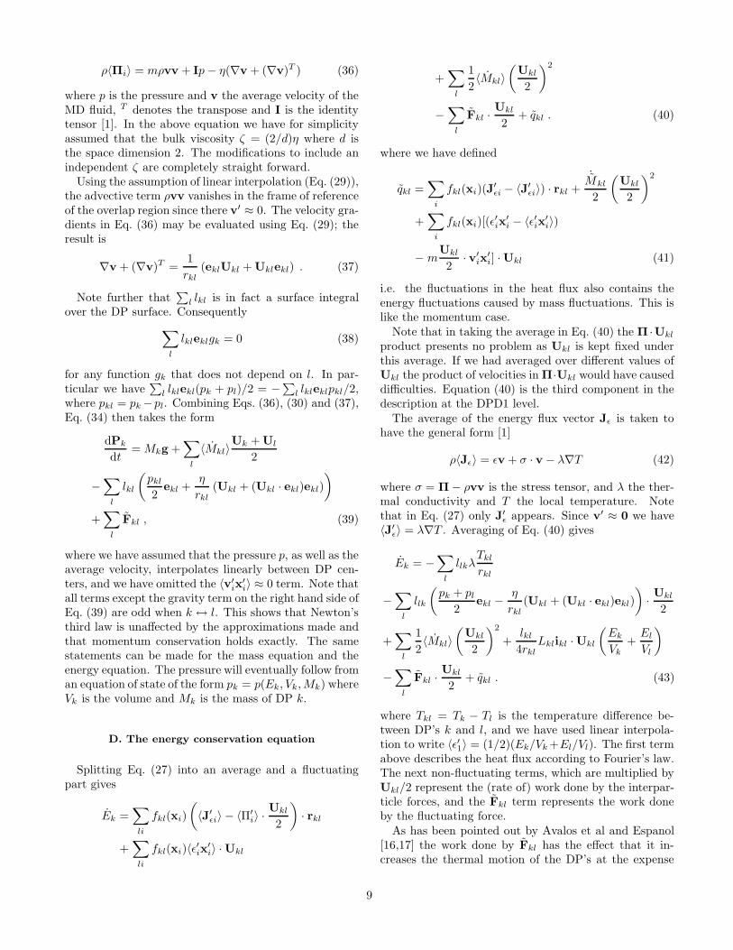
Before we proceed with the derivation of the equationsof motion it is instructive to work out the actual forms offk(x) and fkl(x) in the case of only two particles k andl. Using the Gaussian choice of s we immediately get

fk(x) =1

1 + [exp ((x − (rk + rl)/2) · (rkl)/(a2))]2. (11)

The overlap function similarly follows:

fkl(x) =1

2a2cosh−2

((

x − rk + rl

2

)

·(rkl

a2

)

)

. (12)

l

fk

fkl

lk

k l

k)

)

r

1

rr

r

r

r

k/|r - r |2

l

(r

(r

l

a

kl

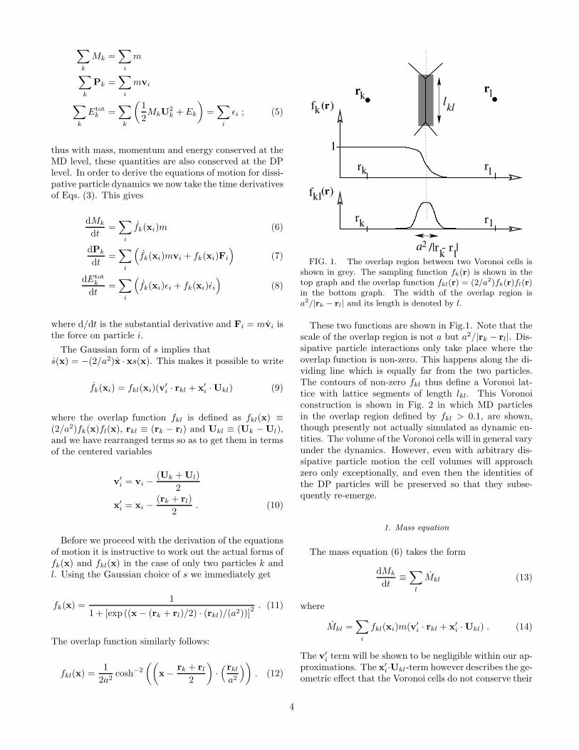
FIG. 1. The overlap region between two Voronoi cells isshown in grey. The sampling function fk(r) is shown in thetop graph and the overlap function fkl(r) = (2/a2)fk(r)fl(r)in the bottom graph. The width of the overlap region isa2/|rk − rl| and its length is denoted by l.

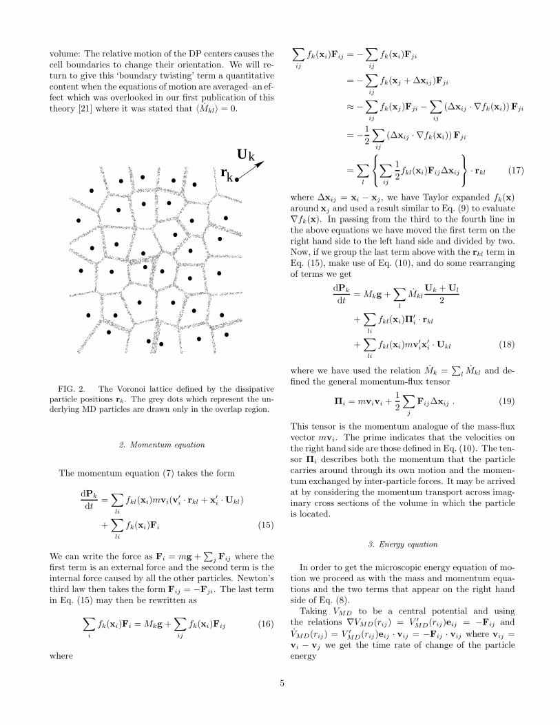
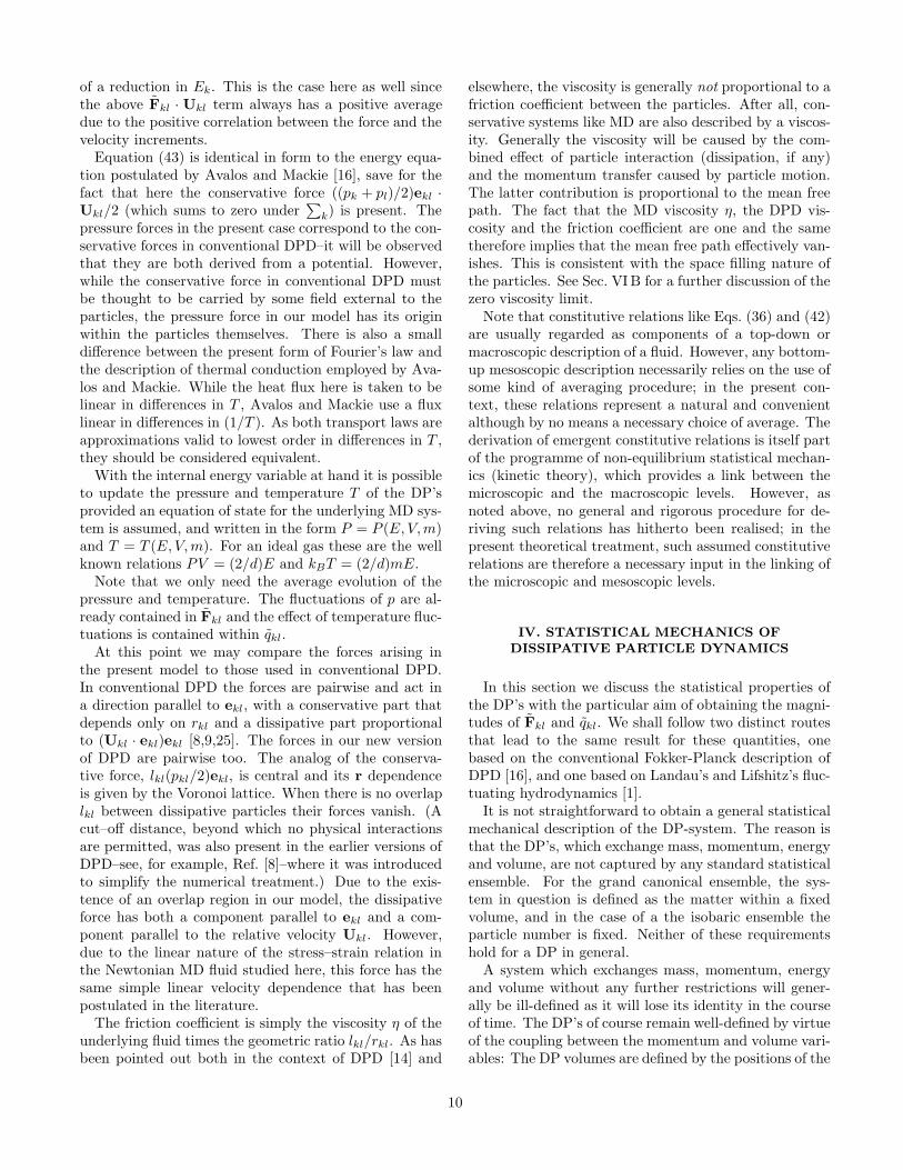
These two functions are shown in Fig.1. Note that thescale of the overlap region is not a but a2/|rk − rl|. Dis-sipative particle interactions only take place where theoverlap function is non-zero. This happens along the di-viding line which is equally far from the two particles.The contours of non-zero fkl thus define a Voronoi lat-tice with lattice segments of length lkl. This Voronoiconstruction is shown in Fig. 2 in which MD particlesin the overlap region defined by fkl > 0.1, are shown,though presently not actually simulated as dynamic en-tities. The volume of the Voronoi cells will in general varyunder the dynamics. However, even with arbitrary dis-sipative particle motion the cell volumes will approachzero only exceptionally, and even then the identities ofthe DP particles will be preserved so that they subse-quently re-emerge.

1. Mass equation

The mass equation (6) takes the form

dMk

dt≡∑

l

Mkl (13)

where

Mkl =∑

i

fkl(xi)m(v′i · rkl + x′

i · Ukl) . (14)

The v′i term will be shown to be negligible within our ap-

proximations. The x′i·Ukl-term however describes the ge-

ometric effect that the Voronoi cells do not conserve their

4

volume: The relative motion of the DP centers causes thecell boundaries to change their orientation. We will re-turn to give this ‘boundary twisting’ term a quantitativecontent when the equations of motion are averaged–an ef-fect which was overlooked in our first publication of thistheory [21] where it was stated that 〈Mkl〉 = 0.

rk

Uk

FIG. 2. The Voronoi lattice defined by the dissipativeparticle positions rk. The grey dots which represent the un-derlying MD particles are drawn only in the overlap region.

2. Momentum equation

The momentum equation (7) takes the form

dPk

dt=∑

li

fkl(xi)mvi(v′i · rkl + x′

i ·Ukl)

+∑

li

fk(xi)Fi (15)

We can write the force as Fi = mg +∑

j Fij where thefirst term is an external force and the second term is theinternal force caused by all the other particles. Newton’sthird law then takes the form Fij = −Fji. The last termin Eq. (15) may then be rewritten as

∑

i

fk(xi)Fi = Mkg +∑

ij

fk(xi)Fij (16)

where

∑

ij

fk(xi)Fij = −∑

ij

fk(xi)Fji

= −∑

ij

fk(xj + ∆xij)Fji

≈ −∑

ij

fk(xj)Fji −∑

ij

(∆xij · ∇fk(xi))Fji

= −1

2

∑

ij

(∆xij · ∇fk(xi))Fji

=∑

l

∑

ij

1

2fkl(xi)Fij∆xij

· rkl (17)

where ∆xij = xi − xj , we have Taylor expanded fk(x)around xj and used a result similar to Eq. (9) to evaluate∇fk(x). In passing from the third to the fourth line inthe above equations we have moved the first term on theright hand side to the left hand side and divided by two.Now, if we group the last term above with the rkl term inEq. (15), make use of Eq. (10), and do some rearrangingof terms we get

dPk

dt= Mkg +

∑

l

MklUk + Ul

2

+∑

li

fkl(xi)Π′i · rkl

+∑

li

fkl(xi)mv′ix

′i · Ukl (18)

where we have used the relation Mk =∑

l Mkl and de-fined the general momentum-flux tensor

Πi = mvivi +1

2

∑

j

Fij∆xij . (19)

This tensor is the momentum analogue of the mass-fluxvector mvi. The prime indicates that the velocities onthe right hand side are those defined in Eq. (10). The ten-sor Πi describes both the momentum that the particlecarries around through its own motion and the momen-tum exchanged by inter-particle forces. It may be arrivedat by considering the momentum transport across imag-inary cross sections of the volume in which the particleis located.

3. Energy equation

In order to get the microscopic energy equation of mo-tion we proceed as with the mass and momentum equa-tions and the two terms that appear on the right handside of Eq. (8).

Taking VMD to be a central potential and usingthe relations ∇VMD(rij) = V ′

MD(rij)eij = −Fij and

VMD(rij) = V ′MD(rij)eij · vij = −Fij · vij where vij =

vi − vj we get the time rate of change of the particleenergy

5

εi = mg · vi +1

2

∑

j 6=i

Fij · (vi + vj) . (20)

This gives the first term of Eq. (8) in the form

∑

i

fk(xi)ε = Pk · g +1

2

∑

i6=j

fk(xi)Fij · (vi + vj) . (21)

The last term of this equation is odd under the exchangei ↔ j and exactly the same manipulations as in Eq. (17)may be used to give

∑

i

fk(xi)ε = Pk · g

+∑

l,i6=j

fkl(xi)1

4Fij · (vi + vj)∆xij · rkl

= Pk · g +∑

l,i6=j

fkl(xi)

(

1

4Fij · (v′

i + v′j)

+1

2Fij ·

Uk + Ul

2

)

∆xij · rkl (22)

where for later purposes we have used Eqs. (10) to get thelast equation. The last term of Eq. (8) is easily writtendown using Eq. (9). This gives

∑

i

fk(xi)εi =∑

li

fkl(xi)(v′i · rkl + x′

i · Ukl)εi . (23)

As previously we write the particle velocities in terms ofv′

i. The corresponding expression for the particle energyis εi = ε′i + mv′

i · (Uk + Ul)/2 + (1/2)m((Uk + Ul)/2)2

where the prime in ε′i denotes that the particle velocityis v′

i rather than vi. Equation (23) may then be written

∑

i

fk(xi)εi =∑

l

1

2Mkl

(

Uk + Ul

2

)2

+∑

li

fkl(xi)

(

ε′iv′i + mv′

iv′i ·

Uk + Ul

2

)

· rkl

+∑

li

fkl(xi)εix′i ·Ukl . (24)

Combining this equation with Eq. (22) we obtain

Etotk =

∑

li

fkl(xi)

(

J′εi + Π′

i ·Uk + Ul

2

)

· rkl

+ MkUk · g +∑

l

1

2Mkl

(

Uk + Ul

2

)2

+∑

li

fkl(xi)

(

ε′i + mv′i ·(

Uk + Ul

2

))

x′i · Ukl . (25)

where the momentum-flux tensor is defined in Eq. (19)and we have identified the energy-flux vector associatedwith a particle i

Jεi = εivi +1

4

∑

i6=j

Fij · (vi + vj)∆xij . (26)

Again the prime denotes that the velocities are v′i rather

than vi. To get the internal energy Ek instead of Etotk we

note that d(P2k/2Mk)/dt = Uk · Pk − (1/2)MkU

2k. Using

this relation, the momentum equation Eq. (18), as well asthe substitution (Uk + Ul)/2 = Uk −Ukl/2 in Eq. (25),followed by some rearrangement of the Mkl terms we findthat

Etotk =

d

dt

(

1

2MkU

2k

)

+∑

l

1

2Mkl

(

Ukl

2

)2

+∑

li

fkl(xi)

(

J′εi − Π′

i ·Ukl

2

)

· rkl

+∑

li

fkl(xi)

(

ε′i − mv′i ·

Ukl

2

)

x′i · Ukl . (27)

This equation has a natural physical interpretation.The first term represents the translational kinetic energyof the DP as a whole. The remaining terms representthe internal energy Ek. This is a purely thermodynamicquantity which cannot depend on the overall velocity ofthe DP, i.e. it must be Galilean invariant. This is eas-ily checked as the relevant terms all depend on velocitydifferences only.

The Mkl term represents the kinetic energy receivedthrough mass exchange with neighboring DPs. As willbecome evident when we turn to the averaged descrip-tion, the term involving the momentum and energy fluxesrepresents the work done on the DP by its neighbors andthe heat conducted from them. The ε′i-term representsthe energy received by the DP due to the same ‘bound-ary twisting’ effect that was found in the mass equation.Upon averaging, the last term proportional to v′

i will beshown to be relatively small since 〈v′

i〉 = 0 in our approx-imations. This is true also in the mass and momentumequations. Equations (14), (18) and (27) have the coarsegrained form that will remain in the final DPD equations.Note, however, that they retain the full microscopic in-formation about the MD system, and for that reason theyare time-reversible. Equation (18) for instance containsonly terms of even order in the velocity. In the next sec-tion terms of odd order will appear when this equationis averaged.

It can be seen that the rate of change of momentumin Eq. (18) is given as a sum of separate pairwise con-tributions from the other particles, and that these termsare all odd under the exchange l ↔ k. Thus the parti-cles interact in a pairwise fashion and individually fulfillNewton’s third law; in other words, momentum conser-vation is again explicitly upheld. The same symmetrieshold for the mass conservation equation (14) and energyequation (25).

6

III. DERIVATION OF DISSIPATIVE PARTICLE

DYNAMICS: AVERAGE AND FLUCTUATING

FORCES

We can now investigate the average and fluctuatingparts of Eqs. (27), (18) and (14). In so doing we shallneed to draw on a hydrodynamic description of the un-derlying molecular dynamics and construct a statisticalmechanical description of our dissipative particle dynam-ics. For concreteness we shall take the hydrodynamic de-scription of the MD system in question to be that of asimple Newtonian fluid [1]. This is known to be a gooddescription for MD fluids based on Lennard-Jones or hardsphere potentials, particularly in three dimensions [3].Here we shall carry out the analysis for systems in twospatial dimensions; the generalization to three dimen-sions is straight forward, the main difference being ofa practical nature as the Voronoi construction becomesmore involved.

We shall begin by specifying a scale separation betweenthe dissipative particles and the molecular dynamics par-ticles by assuming that

|xi − xj | << |rk − rl| , (28)

where xi and xj denote the positions of neighbouring MDparticles. Such a scale separation is in general necessaryin order for the coarse-graining procedure to be physi-cally meaningful. Although for the most part in this pa-per we are thinking of the molecular interactions as beingmediated by short-range forces such as those of Lennard-Jones type, a local description of the interactions will stillbe valid for the case of long-range Coulomb interactionsin an electrostatically neutral system, provided that thescreening length is shorter than the width of the over-lap region between the dissipative particles. Indeed, aswe shall show here, the result of doing a local averag-ing is that the original Newtonian equations of motionfor the MD system become a set of Langevin equationsfor the dissipative particle dynamics. These Langevinequations admit an associated Fokker-Planck equation.An associated fluctuation-dissipation relation relates theamplitude of the Langevin force to the temperature anddamping in the system.

A. Definition of ensemble averages

With the mesoscopic variables now available, we needto define the correct average corresponding to a dynam-ical state of the system. Many MD configurations areconsistent with a given value of the set {rk, Mk,Uk, Ek},and averages are computed by means of an ensemble ofsystems with common instantaneous values of the set{rk, Mk,Uk, Ek}. This means that only the time deriva-tives of the set {rk, Mk,Uk, Ek}, i.e. the forces, have a

fluctuating part. In the end of our development approxi-mate distributions for Uk’s and Ek’s will follow from thederived Fokker-Planck equations. These distributions re-fer to the larger equilibrium ensemble that contains allfluctuations in {rk, Mk,Uk, Ek}.

It is necessary, to compute the average MD particlevelocity 〈v〉 between dissipative particle centers, given{rk, Mk,Uk, Ek}. This velocity depends on all neighbor-ing dissipative particle velocities. However, for simplicitywe shall only employ a “nearest neighbor” approxima-tion, which consists in assuming that 〈v〉 interpolates lin-early between the two nearest dissipative particles. Thisapproximation is of the same nature as the approxima-tion used in the Newtonian fluid stress–strain relationwhich is linear in the velocity gradient. This implies thatin the overlap region between dissipative particles k andl

〈v′〉 = 〈v′〉(x) =x′ · rkl

r2kl

Ukl , (29)

where the primes are defined in Eqs. (10) and rkl =|rk − rl|.

A preliminary mathematical observation is useful insplitting the equations of motion into average and fluc-tuating parts. Let r(x) be an arbitrary, slowly varyingfunction on the a2/rkl scale. Then we shall employ theapproximation corresponding to a linear interpolation be-tween DP centers, that r(x) = (1/2)(rk + rl) where x isa position in the overlap region between DP k and l andrk and rl are values of the function r associated with theDP centers k and l respectively.

x

y

kleikl

Lkl

l k

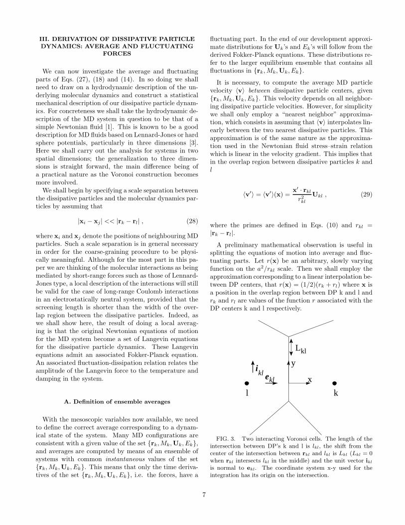
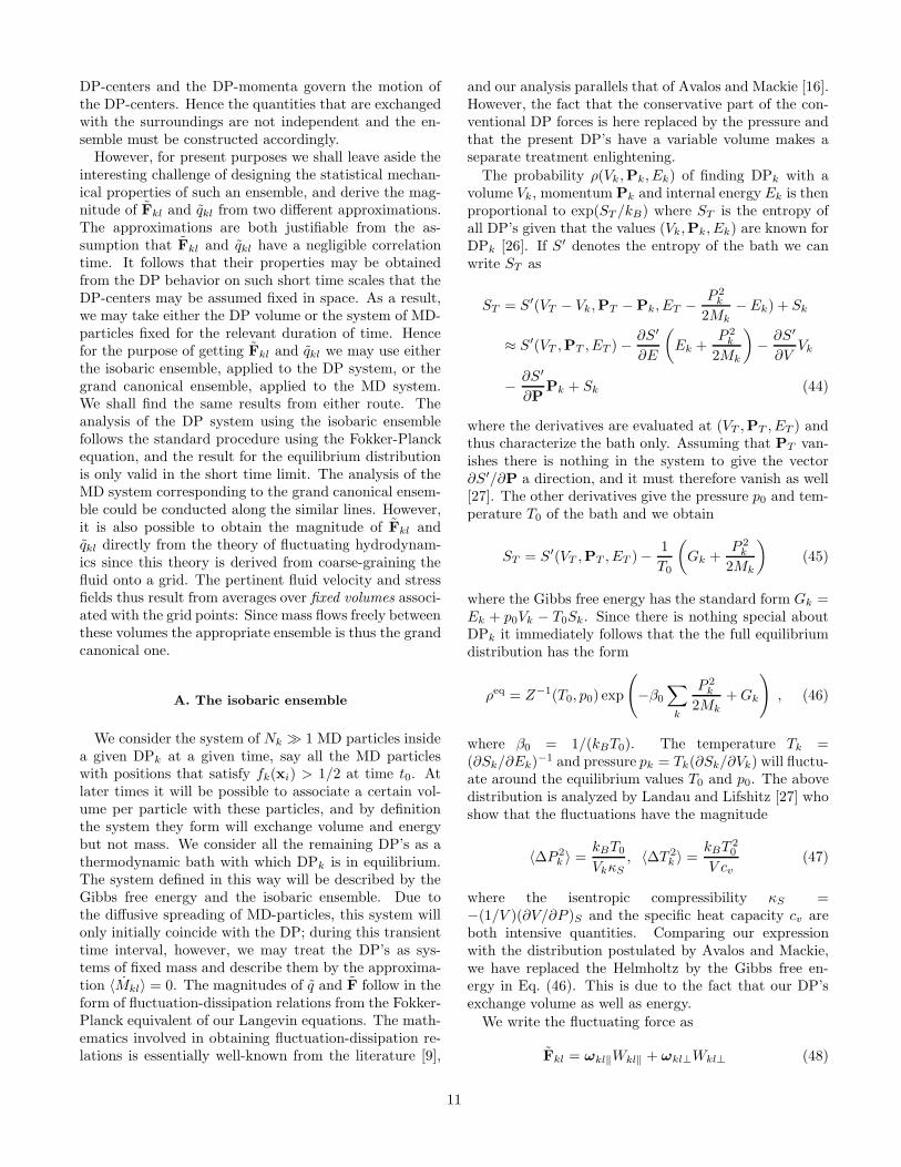
FIG. 3. Two interacting Voronoi cells. The length of theintersection between DP’s k and l is lkl, the shift from thecenter of the intersection between rkl and lkl is Lkl (Lkl = 0when rkl intersects lkl in the middle) and the unit vector ikl

is normal to ekl. The coordinate system x-y used for theintegration has its origin on the intersection.

7

Then

∑

i fkl(xi)r(x) ≈∫

dx dyρk + ρl

2fkl(x)

rk + rl

2

≈ lkl

2a2

ρk + ρl

2

rk + rl

2

∫ ∞

−∞

dx′ cosh−2 (x′rkl/a2)

=lkl

rkl

ρk + ρl

2

rk + rl

2, (30)

where ρk+ρl

2is the MD particle number density and we

have used the identity tanh′(x) = cosh−2(x). We willalso need the first moment in x′

∑

i

fkl(xi)x′ir(xi) ≈

∫

dxdyρk + ρl

2fkl(x)x′ rk + rl

2

≈ 1

2a2

ρk + ρl

2

rk + rl

2

∫

dx dy cosh−2(xrkl

a2

)

yikl

=lkl

2rklLkl

ρk + ρl

2

rk + rl

2ikl (31)

where the unit vectors ekl = rkl/rkl and ikl are shownin Fig. 3, we have used the fact that the integralover xekl cosh−2 ... vanishes since the integrand is odd,and the last equation follows by the substitution x →(a2/rkl)x. In contrast to the vector ekl the vector ikl iseven under the exchange k ↔ l, as is Lkl. This is a mat-ter of definition only as it would be equally permissibleto let ikl and Lkl be odd under this exchange. However,it is important for the symmetry properties of the fluxesthat ikl and Lkl have the same symmetry under k ↔ l.

B. The mass conservation equation

Taking the average of Eq. (14), we observe that thefirst term vanishes if Eq. (29) is used, and the secondterm follows directly from Eq. (31). We thus obtain

Mk =∑

l

(〈Mkl〉 + ˙Mkl) (32)

where

〈Mkl〉 =∑

li

fklm(xi)〈x′i〉 · Ukl =

lkl

2rklLkl

ρk + ρl

2ikl · Ukl ,

(33)

and ˙Mkl = Mkl − 〈Mkl〉. The finite value of 〈Mkl〉 iscaused by the relative DP motion perpendicular to ekl.This is a geometric effect intrinsic to the Voronoi lat-tice. When particles move the Voronoi boundaries changetheir orientation, and this boundary twisting causes massto be transferred between DP’s. This mass variation willbe visible in the energy flux, though not in the momen-tum flux. It will later be shown that the effect of massfluctuations in the momentum and energy equations maybe absorbed in the force and heat flux fluctuations.

C. The momentum conservation equation

Using Eq. (33) we may split Eq. (18) into average andfluctuating parts to get

dPk

dt= Mkg

+∑

l

〈Mkl〉Uk + Ul

2+∑

li

fkl(xi)〈Πi〉 · rkl

+∑

i

fkl(xi)m〈v′ix

′i〉 · Ukl +

∑

l

Fkl , (34)

where the fluctuating force or, equivalently, the momen-tum flux is

Fkl =∑

i

fkl(xi)[(Πi − 〈Πi〉) · rkl

+ m(v′ix

′i − 〈v′

ix′i〉) ·Ukl]

+ ˙MklUk + Ul

2. (35)

Note that by definition Flk = −Fkl. The fact that wehave absorbed mass fluctuations with the fluctuations inFkl deserves a comment. In general force fluctuationswill cause mass fluctuations, which in turn will coupleback to cause momentum fluctuations. The time scaleover which this will happen is tη = r2

kl/η, where η is thedynamic viscosity of the MD system. This is the timeit takes for a velocity perturbation to decay over a dis-tance of rkl. Perturbations mediated by the pressure, i.e.sound waves, will have a shorter time. In the sequel weshall need to make the assumption that the forces areMarkovian, and it is clear that this assumption may onlybe valid on time scales larger than tη. Since the timescale of a hydrodynamic perturbation of size l, say, isalso given as l2/η this restriction implies the scale sepa-ration requirement r2

kl << l2, consistent with the scalerkl being mesoscopic.

Since 〈Πi〉 is in general dissipative in nature, Eq. (34)and its mass- and energy analogue will be referred to asDPD1. It is at the point of taking the average in Eq. (34)that time reversibility is lost. Note, however, that we donot claim to treat the introduction of irreversibility intothe problem in a mathematically rigorous way. This isa very difficult problem in general which so far has onlybeen realized by rigorous methods in the case of somevery simple dynamical systems with well defined ergodicproperties [22–24]. We shall instead use the constitu-tive relation for a Newtonian fluid which, as noted ear-lier, is an emergent property of Lennard-Jones and hardsphere MD systems, to give Eq. (34) a concrete content.The momentum-flux tensor then has the following simpleform

8

ρ〈Πi〉 = mρvv + Ip − η(∇v + (∇v)T ) (36)

where p is the pressure and v the average velocity of theMD fluid, T denotes the transpose and I is the identitytensor [1]. In the above equation we have for simplicityassumed that the bulk viscosity ζ = (2/d)η where d isthe space dimension 2. The modifications to include anindependent ζ are completely straight forward.

Using the assumption of linear interpolation (Eq. (29)),the advective term ρvv vanishes in the frame of referenceof the overlap region since there v′ ≈ 0. The velocity gra-dients in Eq. (36) may be evaluated using Eq. (29); theresult is

∇v + (∇v)T =1

rkl(eklUkl + Uklekl) . (37)

Note further that∑

l lkl is in fact a surface integralover the DP surface. Consequently

∑

l

lkleklgk = 0 (38)

for any function gk that does not depend on l. In par-ticular we have

∑

l lklekl(pk + pl)/2 = −∑

l lkleklpkl/2,where pkl = pk −pl. Combining Eqs. (36), (30) and (37),Eq. (34) then takes the form

dPk

dt= Mkg +

∑

l

〈Mkl〉Uk + Ul

2

−∑

l

lkl

(

pkl

2ekl +

η

rkl(Ukl + (Ukl · ekl)ekl)

)

+∑

l

Fkl , (39)

where we have assumed that the pressure p, as well as theaverage velocity, interpolates linearly between DP cen-ters, and we have omitted the 〈v′

ix′i〉 ≈ 0 term. Note that

all terms except the gravity term on the right hand side ofEq. (39) are odd when k ↔ l. This shows that Newton’sthird law is unaffected by the approximations made andthat momentum conservation holds exactly. The samestatements can be made for the mass equation and theenergy equation. The pressure will eventually follow froman equation of state of the form pk = p(Ek, Vk, Mk) whereVk is the volume and Mk is the mass of DP k.

D. The energy conservation equation

Splitting Eq. (27) into an average and a fluctuatingpart gives

Ek =∑

li

fkl(xi)

(

〈J′εi〉 − 〈Π′

i〉 ·Ukl

2

)

· rkl

+∑

li

fkl(xi)〈ε′ix′i〉 · Ukl

+∑

l

1

2〈Mkl〉

(

Ukl

2

)2

−∑

l

Fkl ·Ukl

2+ qkl . (40)

where we have defined

qkl =∑

i

fkl(xi)(J′εi − 〈J′

εi〉) · rkl +˙Mkl

2

(

Ukl

2

)2

+∑

i

fkl(xi)[(ε′ix

′i − 〈ε′ix′

i〉)

− mUkl

2· v′

ix′i] ·Ukl (41)

i.e. the fluctuations in the heat flux also contains theenergy fluctuations caused by mass fluctuations. This islike the momentum case.

Note that in taking the average in Eq. (40) the Π ·Ukl

product presents no problem as Ukl is kept fixed underthis average. If we had averaged over different values ofUkl the product of velocities in Π·Ukl would have causeddifficulties. Equation (40) is the third component in thedescription at the DPD1 level.

The average of the energy flux vector Jε is taken tohave the general form [1]

ρ〈Jε〉 = εv + σ · v − λ∇T (42)

where σ = Π− ρvv is the stress tensor, and λ the ther-mal conductivity and T the local temperature. Notethat in Eq. (27) only J′

ε appears. Since v′ ≈ 0 we have〈J′

ε〉 = λ∇T . Averaging of Eq. (40) gives

Ek = −∑

l

llkλTkl

rkl

−∑

l

llk

(

pk + pl

2ekl −

η

rkl(Ukl + (Ukl · ekl)ekl)

)

· Ukl

2

+∑

l

1

2〈Mkl〉

(

Ukl

2

)2

+lkl

4rklLklikl ·Ukl

(

Ek

Vk+

El

Vl

)

−∑

l

Fkl ·Ukl

2+ qkl . (43)

where Tkl = Tk − Tl is the temperature difference be-tween DP’s k and l, and we have used linear interpola-tion to write 〈ε′1〉 = (1/2)(Ek/Vk +El/Vl). The first termabove describes the heat flux according to Fourier’s law.The next non-fluctuating terms, which are multiplied byUkl/2 represent the (rate of) work done by the interpar-ticle forces, and the Fkl term represents the work doneby the fluctuating force.

As has been pointed out by Avalos et al and Espanol[16,17] the work done by Fkl has the effect that it in-creases the thermal motion of the DP’s at the expense

9

of a reduction in Ek. This is the case here as well sincethe above Fkl · Ukl term always has a positive averagedue to the positive correlation between the force and thevelocity increments.

Equation (43) is identical in form to the energy equa-tion postulated by Avalos and Mackie [16], save for thefact that here the conservative force ((pk + pl)/2)ekl ·Ukl/2 (which sums to zero under

∑

k) is present. Thepressure forces in the present case correspond to the con-servative forces in conventional DPD–it will be observedthat they are both derived from a potential. However,while the conservative force in conventional DPD mustbe thought to be carried by some field external to theparticles, the pressure force in our model has its originwithin the particles themselves. There is also a smalldifference between the present form of Fourier’s law andthe description of thermal conduction employed by Ava-los and Mackie. While the heat flux here is taken to belinear in differences in T , Avalos and Mackie use a fluxlinear in differences in (1/T ). As both transport laws areapproximations valid to lowest order in differences in T ,they should be considered equivalent.

With the internal energy variable at hand it is possibleto update the pressure and temperature T of the DP’sprovided an equation of state for the underlying MD sys-tem is assumed, and written in the form P = P (E, V, m)and T = T (E, V, m). For an ideal gas these are the wellknown relations PV = (2/d)E and kBT = (2/d)mE.

Note that we only need the average evolution of thepressure and temperature. The fluctuations of p are al-ready contained in Fkl and the effect of temperature fluc-tuations is contained within qkl.

At this point we may compare the forces arising inthe present model to those used in conventional DPD.In conventional DPD the forces are pairwise and act ina direction parallel to ekl, with a conservative part thatdepends only on rkl and a dissipative part proportionalto (Ukl · ekl)ekl [8,9,25]. The forces in our new versionof DPD are pairwise too. The analog of the conserva-tive force, lkl(pkl/2)ekl, is central and its r dependenceis given by the Voronoi lattice. When there is no overlaplkl between dissipative particles their forces vanish. (Acut–off distance, beyond which no physical interactionsare permitted, was also present in the earlier versions ofDPD–see, for example, Ref. [8]–where it was introducedto simplify the numerical treatment.) Due to the exis-tence of an overlap region in our model, the dissipativeforce has both a component parallel to ekl and a com-ponent parallel to the relative velocity Ukl. However,due to the linear nature of the stress–strain relation inthe Newtonian MD fluid studied here, this force has thesame simple linear velocity dependence that has beenpostulated in the literature.

The friction coefficient is simply the viscosity η of theunderlying fluid times the geometric ratio lkl/rkl. As hasbeen pointed out both in the context of DPD [14] and

elsewhere, the viscosity is generally not proportional to afriction coefficient between the particles. After all, con-servative systems like MD are also described by a viscos-ity. Generally the viscosity will be caused by the com-bined effect of particle interaction (dissipation, if any)and the momentum transfer caused by particle motion.The latter contribution is proportional to the mean freepath. The fact that the MD viscosity η, the DPD vis-cosity and the friction coefficient are one and the sametherefore implies that the mean free path effectively van-ishes. This is consistent with the space filling nature ofthe particles. See Sec. VI B for a further discussion of thezero viscosity limit.

Note that constitutive relations like Eqs. (36) and (42)are usually regarded as components of a top-down ormacroscopic description of a fluid. However, any bottom-up mesoscopic description necessarily relies on the use ofsome kind of averaging procedure; in the present con-text, these relations represent a natural and convenientalthough by no means a necessary choice of average. Thederivation of emergent constitutive relations is itself partof the programme of non-equilibrium statistical mechan-ics (kinetic theory), which provides a link between themicroscopic and the macroscopic levels. However, asnoted above, no general and rigorous procedure for de-riving such relations has hitherto been realised; in thepresent theoretical treatment, such assumed constitutiverelations are therefore a necessary input in the linking ofthe microscopic and mesoscopic levels.

IV. STATISTICAL MECHANICS OF

DISSIPATIVE PARTICLE DYNAMICS

In this section we discuss the statistical properties ofthe DP’s with the particular aim of obtaining the magni-tudes of Fkl and qkl. We shall follow two distinct routesthat lead to the same result for these quantities, onebased on the conventional Fokker-Planck description ofDPD [16], and one based on Landau’s and Lifshitz’s fluc-tuating hydrodynamics [1].

It is not straightforward to obtain a general statisticalmechanical description of the DP-system. The reason isthat the DP’s, which exchange mass, momentum, energyand volume, are not captured by any standard statisticalensemble. For the grand canonical ensemble, the sys-tem in question is defined as the matter within a fixedvolume, and in the case of a the isobaric ensemble theparticle number is fixed. Neither of these requirementshold for a DP in general.

A system which exchanges mass, momentum, energyand volume without any further restrictions will gener-ally be ill-defined as it will lose its identity in the courseof time. The DP’s of course remain well-defined by virtueof the coupling between the momentum and volume vari-ables: The DP volumes are defined by the positions of the

10

DP-centers and the DP-momenta govern the motion ofthe DP-centers. Hence the quantities that are exchangedwith the surroundings are not independent and the en-semble must be constructed accordingly.

However, for present purposes we shall leave aside theinteresting challenge of designing the statistical mechan-ical properties of such an ensemble, and derive the mag-nitude of Fkl and qkl from two different approximations.The approximations are both justifiable from the as-sumption that Fkl and qkl have a negligible correlationtime. It follows that their properties may be obtainedfrom the DP behavior on such short time scales that theDP-centers may be assumed fixed in space. As a result,we may take either the DP volume or the system of MD-particles fixed for the relevant duration of time. Hencefor the purpose of getting Fkl and qkl we may use eitherthe isobaric ensemble, applied to the DP system, or thegrand canonical ensemble, applied to the MD system.We shall find the same results from either route. Theanalysis of the DP system using the isobaric ensemblefollows the standard procedure using the Fokker-Planckequation, and the result for the equilibrium distributionis only valid in the short time limit. The analysis of theMD system corresponding to the grand canonical ensem-ble could be conducted along the similar lines. However,it is also possible to obtain the magnitude of Fkl andqkl directly from the theory of fluctuating hydrodynam-ics since this theory is derived from coarse-graining thefluid onto a grid. The pertinent fluid velocity and stressfields thus result from averages over fixed volumes associ-ated with the grid points: Since mass flows freely betweenthese volumes the appropriate ensemble is thus the grandcanonical one.

A. The isobaric ensemble

We consider the system of Nk � 1 MD particles insidea given DPk at a given time, say all the MD particleswith positions that satisfy fk(xi) > 1/2 at time t0. Atlater times it will be possible to associate a certain vol-ume per particle with these particles, and by definitionthe system they form will exchange volume and energybut not mass. We consider all the remaining DP’s as athermodynamic bath with which DPk is in equilibrium.The system defined in this way will be described by theGibbs free energy and the isobaric ensemble. Due tothe diffusive spreading of MD-particles, this system willonly initially coincide with the DP; during this transienttime interval, however, we may treat the DP’s as sys-tems of fixed mass and describe them by the approxima-tion 〈Mkl〉 = 0. The magnitudes of q and F follow in theform of fluctuation-dissipation relations from the Fokker-Planck equivalent of our Langevin equations. The math-ematics involved in obtaining fluctuation-dissipation re-lations is essentially well-known from the literature [9],

and our analysis parallels that of Avalos and Mackie [16].However, the fact that the conservative part of the con-ventional DP forces is here replaced by the pressure andthat the present DP’s have a variable volume makes aseparate treatment enlightening.

The probability ρ(Vk,Pk, Ek) of finding DPk with avolume Vk, momentum Pk and internal energy Ek is thenproportional to exp(ST /kB) where ST is the entropy ofall DP’s given that the values (Vk,Pk, Ek) are known forDPk [26]. If S′ denotes the entropy of the bath we canwrite ST as

ST = S′(VT − Vk,PT − Pk, ET − P 2k

2Mk− Ek) + Sk

≈ S′(VT ,PT , ET ) − ∂S′

∂E

(

Ek +P 2

k

2Mk

)

− ∂S′

∂VVk

− ∂S′

∂PPk + Sk (44)

where the derivatives are evaluated at (VT ,PT , ET ) andthus characterize the bath only. Assuming that PT van-ishes there is nothing in the system to give the vector∂S′/∂P a direction, and it must therefore vanish as well[27]. The other derivatives give the pressure p0 and tem-perature T0 of the bath and we obtain

ST = S′(VT ,PT , ET ) − 1

T0

(

Gk +P 2

k

2Mk

)

(45)

where the Gibbs free energy has the standard form Gk =Ek + p0Vk − T0Sk. Since there is nothing special aboutDPk it immediately follows that the the full equilibriumdistribution has the form

ρeq = Z−1(T0, p0) exp

(

−β0

∑

k

P 2k

2Mk+ Gk

)

, (46)

where β0 = 1/(kBT0). The temperature Tk =(∂Sk/∂Ek)−1 and pressure pk = Tk(∂Sk/∂Vk) will fluctu-ate around the equilibrium values T0 and p0. The abovedistribution is analyzed by Landau and Lifshitz [27] whoshow that the fluctuations have the magnitude

〈∆P 2k 〉 =

kBT0

VkκS, 〈∆T 2

k 〉 =kBT 2

0

V cv(47)

where the isentropic compressibility κS =−(1/V )(∂V/∂P )S and the specific heat capacity cv areboth intensive quantities. Comparing our expressionwith the distribution postulated by Avalos and Mackie,we have replaced the Helmholtz by the Gibbs free en-ergy in Eq. (46). This is due to the fact that our DP’sexchange volume as well as energy.

We write the fluctuating force as

Fkl = ωkl‖Wkl‖ + ωkl⊥Wkl⊥ (48)

11

where, for reasons soon to become apparent, we havechosen to decompose Fkl into components parallel andperpendicular to ekl. The W ’s are defined as Gaussianrandom variables with the correlation function

〈Wklα(t)Wnmβ(t′)〉 = δαβδ(t − t′)(δknδlm + δkmδln) (49)

where α and β denote either ⊥ or ‖. The product of δfactors ensures that only equal vectorial components ofthe forces between a pair of DP’s are correlated, whileNewton’s third law guarantees that ωkl = −ωlk. Like-wise the fluctuating heat flux takes the form

qkl = ΛklWkl (50)

where Wkl satisfies Eq. (49) without the δαβ factor andenergy conservation implies Λkl = −Λlk.

The force correlation function then takes the form

〈Fkn(t)Flm(t′)〉 = (ωkn⊥ωlm⊥ + ωkn‖ωlm‖)

(δklδnm + δkmδln)δ(t − t′)

≡ ωklnm(δklδnm + δkmδln)δ(t − t′) (51)

where we have introduced the second order tensor ωknlm.It is a standard result in non-equilibrium statistical

mechanics that a Langevin description of a dynamicalvariable y

y = a(y) + G (52)

where G is a delta-correlated force has an equiva-lent probabilistic representation in terms of the Fokker-Planck equation

∂ρ(y, t)

∂t= −∇ · (a(y)ρ(y)) +

1

2∇∇: (A(y)ρ(y)) (53)

where ∇ denotes derivatives with respect to y and ρ(y, t)is the probability distribution for the variable y at timet, 〈G(y, t)G(y, t′)〉 = Aδ(t − t′) and A is a symmetrictensor of rank two [28].

In the preceding paragraph, G denotes all the fluc-tuating terms in Eqs. (39) and (43). Using the abovedefinitions and 〈Mkl〉 = 0 it is a standard matter [9] toobtain the Fokker-Planck equation

∂ρ

∂t= (L0 + LDIS + LDIF), ρ (54)

where

L0 = −∑

k

∂

∂rk·Uk +

∑

k 6=l

lkl

(

∂

∂Pk· ekl

pkl

2

+∂

∂Ekekl · Ukl

pk + pl

4

)

LDIS =∑

k 6=l

lkl

(

∂

∂Pk· FD

kl −∂

∂Ek

(

Ukl

2·FD

kl − λTkl

rkl

))

LDIF =1

2

∑

k 6=l

(

ωklkl ·∂

∂Pk· Lkl −

∂

∂Ek

(

ωklkl ·Ukl

2· Lkl

− Λ2kl

(

∂

∂Ek− ∂

∂El

)))

, (55)

FDkl = (η/rkl)(Ukl + (Ukl · ekl)ekl), and the sum

∑

k 6=l

runs over both k and l. The operator Lkl is defined as inRef. [16]:

Lkl =

(

∂

∂Pk− ∂

∂Pl

)

− Ukl

2

(

∂

∂Ek− ∂

∂El

)

. (56)

The steady-state solution of Eq. (54) is already givenby Eq. (46); following conventional procedures we canobtain the fluctuation-dissipation relations for ω and Λby inserting ρeq in Eq. (54).

Apart from the tensorial nature of ωklkl the operatorsLDIS and LDIF are essentially identical to those publishedearlier in conventional DPD [16,17]. However, the ‘Liou-ville’ operator L0 plays a somewhat different role as itcontains the ∂/∂Ek term, corresponding to the fact thatthe pressure forces do work on the DP’s to change theirinternal energy.

While L0ρeq conventionally vanishes exactly by con-

struction of the inter-DP forces, here it vanishes only toorder 1/Nk. In order to evaluate L0ρ

eq we need the fol-lowing relationship

∂

∂rk=

1

2

∑

k 6=l

lklekl

(

∂

∂Vl− ∂

∂Vk

)

, (57)

which is derived by direct geometrical consideration ofthe Voronoi construction. By repeated use of Eq. (38) itis then a straightforward algebraic task to obtain

L0ρeq =

ρeq

4

∑

k 6=l

lklekl · Uk

[

∂pl

∂El− pklTkl

kBTkTl

]

, (58)

which does not vanish identically. However, note thatif we estimate El ≈ NlkBT we obtain ∂pl/∂El ≈(1/Nk)(pl/kBT ). Similarly we may estimate pkl and Tkl

from Eq. (47) to obtain

pklTkl

kBTkTl≈

√∆P 2∆T 2

kBTkTl=

1

Nk

√

Nk/Vk

κScvT 20

. (59)

The last square root is an intensive quantity of the or-der p0/(kBT0), as may be easily demonstrated for thecase of an ideal gas. Since each separate quantity thatis contained in the differences in the square brackets ofEq. (58) is of the order p0/T0 we have shown that theycancel up to relative order 1/Nk � 1. In fact, it is notsurprising that Langevin equations which approximatelocal gradients to first order only in the correspondingdifferences, like Tkl, give rise to a Fokker-Planck descrip-tion that contains higher order correction terms.

12

Having shown that L0ρeq vanishes to a good ap-

proximation we may proceed to obtain the fluctuation-dissipation relations from the equation (LDIS +LDIF)ρeq = 0. It may be noted from Eq. (55) that thisequation is satisfied if

(lklFDkl +

1

2ωklklLkl)ρ

eq = 0(

lklλTkl

rkl+

1

2Λ2

kl

(

∂

∂Ek− ∂

∂El

))

ρeq = 0 . (60)

Using the identity

eklekl + iklikl = I (61)

where ikl a vector normal to ekl, we may show thatEq. (60) implies that

ω2kl‖ = 2ω2

kl⊥ = 4ηkBΘkllkl

rkl

Λ2kl = 2kBTkTlλ

lkl

rkl, (62)

where Θ−1kl = (1/2)(T−1

k + T−1l ).

B. F from fluctuating hydrodynamics

Having derived the fluctuation-dissipation relationsfrom the approximation of the isobaric ensemble we nowderive the same result from fluctuating hydrodynamics,which corresponds to the grand canonical ensemble. Weshall only derive the magnitude of Fkl since q follows onthe basis of the same reasoning.

Fluctuating hydrodynamics [1] is based on the conser-vation equations for mass, momentum and energy withthe modification that the momentum and energy fluxescontain an additional fluctuating term. Specifically, themomentum flux tensor takes the form −∇P + ρvv + σ′,where P is the pressure, v is the velocity field and theviscous stress tensor is given as

σ′ = η

(

∇v + ∇vT − 2

d∇ · v

)

+ ζ∇ · v + s, (63)

where s is the fluctuating component of the momentumflux. From the same approximations as we used in de-riving Eq. (62), i.e. a negligible correlation time for thefluctuating forces, Landau and Lifshitz derive

〈s(x, t) · ns(x′, 0) · n〉 = 2kBT

(

η(1 + nn) + (ζ − 2

dη)nn

)

δ(t)

{

1∆Vn

if x,x′ε∆Vn

0 otherwise(64)

where n is an arbitrary unit vector and n labels the vol-ume element ∆Vn. By following the derivations presented

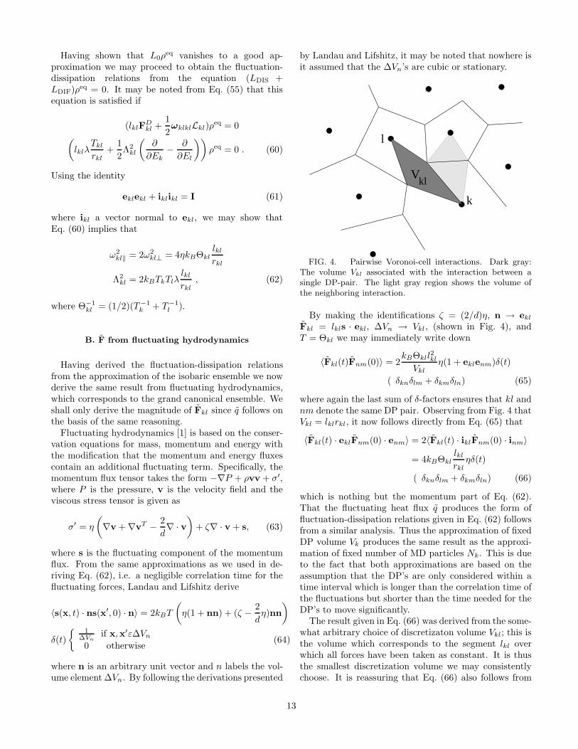
by Landau and Lifshitz, it may be noted that nowhere isit assumed that the ∆Vn’s are cubic or stationary.

l

k

Vkl

FIG. 4. Pairwise Voronoi-cell interactions. Dark gray:The volume Vkl associated with the interaction between asingle DP-pair. The light gray region shows the volume ofthe neighboring interaction.

By making the identifications ζ = (2/d)η, n → ekl

Fkl = lkls · ekl, ∆Vn → Vkl, (shown in Fig. 4), andT = Θkl we may immediately write down

〈Fkl(t)Fnm(0)〉 = 2kBΘkll

2kl

Vklη(1 + eklenm)δ(t)

( δknδlm + δkmδln) (65)

where again the last sum of δ-factors ensures that kl andnm denote the same DP pair. Observing from Fig. 4 thatVkl = lklrkl, it now follows directly from Eq. (65) that

〈Fkl(t) · eklFnm(0) · enm〉 = 2〈Fkl(t) · iklFnm(0) · inm〉

= 4kBΘkllkl

rklηδ(t)

( δknδlm + δkmδln) (66)

which is nothing but the momentum part of Eq. (62).That the fluctuating heat flux q produces the form offluctuation-dissipation relations given in Eq. (62) followsfrom a similar analysis. Thus the approximation of fixedDP volume Vk produces the same result as the approxi-mation of fixed number of MD particles Nk. This is dueto the fact that both approximations are based on theassumption that the DP’s are only considered within atime interval which is longer than the correlation time ofthe fluctuations but shorter than the time needed for theDP’s to move significantly.

The result given in Eq. (66) was derived from the some-what arbitrary choice of discretizaton volume Vkl; this isthe volume which corresponds to the segment lkl overwhich all forces have been taken as constant. It is thusthe smallest discretization volume we may consistentlychoose. It is reassuring that Eq. (66) also follows from

13

different choices of ∆Vn. For example, one may readilycheck that Eq. (66) is obtained if we split Vkl in two alongrkl and consider Fkl to be the sum of two independentforces acting on the two parts of lkl.

We are now in a position to quantify the av-

erage component 〈 ˙Ek〉 ≡ ∑

l6=k〈Fkl · Ukl/2〉 ofthe fluctuations in the internal energy given inEq. (43). Writing the velocity in response to Fkl as

Uk =∑

l 6=k

∫ t

−∞ dt′Fkl(t′)/Mk, we get that 〈 ˙Ek〉 =

∑∫ t

−∞ dt′〈Fkl(t′)Fkl(t)〉 which by Eqs. (62) and (51) be-

comes 〈 ˙Ek〉 = (1/Mk)∑

3lklηkBΘkl/rkl. This result isthe same as one would have obtained applying the rules ofIto calculus to U2

k/(2Mk). It yields the modified, thoughequivalent, energy equation

Ek = −∑

l

llkλTkl

rkl

−∑

l

llk

(

pk + pl

2ekl −

η

rkl(Ukl + (Ukl · ekl)ekl)

)

· Ukl

2

−∑

l

F′kl ·

Ukl

2− 3

lkl

rklηkBΘkl + qkl . (67)

where we have written F′kl with a prime to denote that

it is uncorrelated with Ukl. In a numerical implemen-tation this implies that F′

kl must be generated from adifferent random variable than Fkl, which was used toupdate Ukl.

The fluctuation-dissipation relations Eqs. (62) com-plete our theoretical description of dissipative particledynamics, which has been derived by a coarse-grainingof molecular dynamics. All the parameters and proper-ties of this new version of DPD are related directly tothe underlying molecular dynamics, and properties suchas the viscosity which are emergent from it.

V. SIMULATIONS

While the present paper primarily deals with theoreti-cal developments we have carried out simulations to testthe equilibrium behavior of the model in the case of theisothermal model. This is a crucial test as the deriva-tion of the fluctuating forces relies on the most signif-icant approximations. The simulations are carried outusing a periodic Voronoi tesselation described in detailelsewhere [29].

500 1000 1500 2000 2500 3000 3500 40000

0.2

0.4

0.6

0.8

1

Tem

per

atu

re (

k BT

)

Iterations

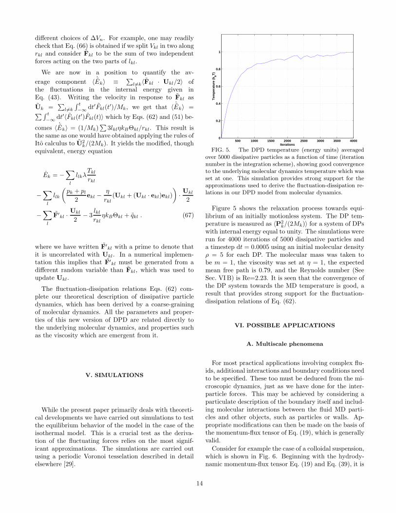
FIG. 5. The DPD temperature (energy units) averagedover 5000 dissipative particles as a function of time (iterationnumber in the integration scheme), showing good convergenceto the underlying molecular dynamics temperature which wasset at one. This simulation provides strong support for theapproximations used to derive the fluctuation-dissipation re-lations in our DPD model from molecular dynamics.

Figure 5 shows the relaxation process towards equi-librium of an initially motionless system. The DP tem-perature is measured as 〈P2

k/(2Mk)〉 for a system of DPswith internal energy equal to unity. The simulations wererun for 4000 iterations of 5000 dissipative particles anda timestep dt = 0.0005 using an initial molecular densityρ = 5 for each DP. The molecular mass was taken tobe m = 1, the viscosity was set at η = 1, the expectedmean free path is 0.79, and the Reynolds number (SeeSec. VI B) is Re=2.23. It is seen that the convergence ofthe DP system towards the MD temperature is good, aresult that provides strong support for the fluctuation-dissipation relations of Eq. (62).

VI. POSSIBLE APPLICATIONS

A. Multiscale phenomena

For most practical applications involving complex flu-ids, additional interactions and boundary conditions needto be specified. These too must be deduced from the mi-croscopic dynamics, just as we have done for the inter-particle forces. This may be achieved by considering aparticulate description of the boundary itself and includ-ing molecular interactions between the fluid MD parti-cles and other objects, such as particles or walls. Ap-propriate modifications can then be made on the basis ofthe momentum-flux tensor of Eq. (19), which is generallyvalid.

Consider for example the case of a colloidal suspension,which is shown in Fig. 6. Beginning with the hydrody-namic momentum-flux tensor Eq. (19) and Eq. (39), it is

14

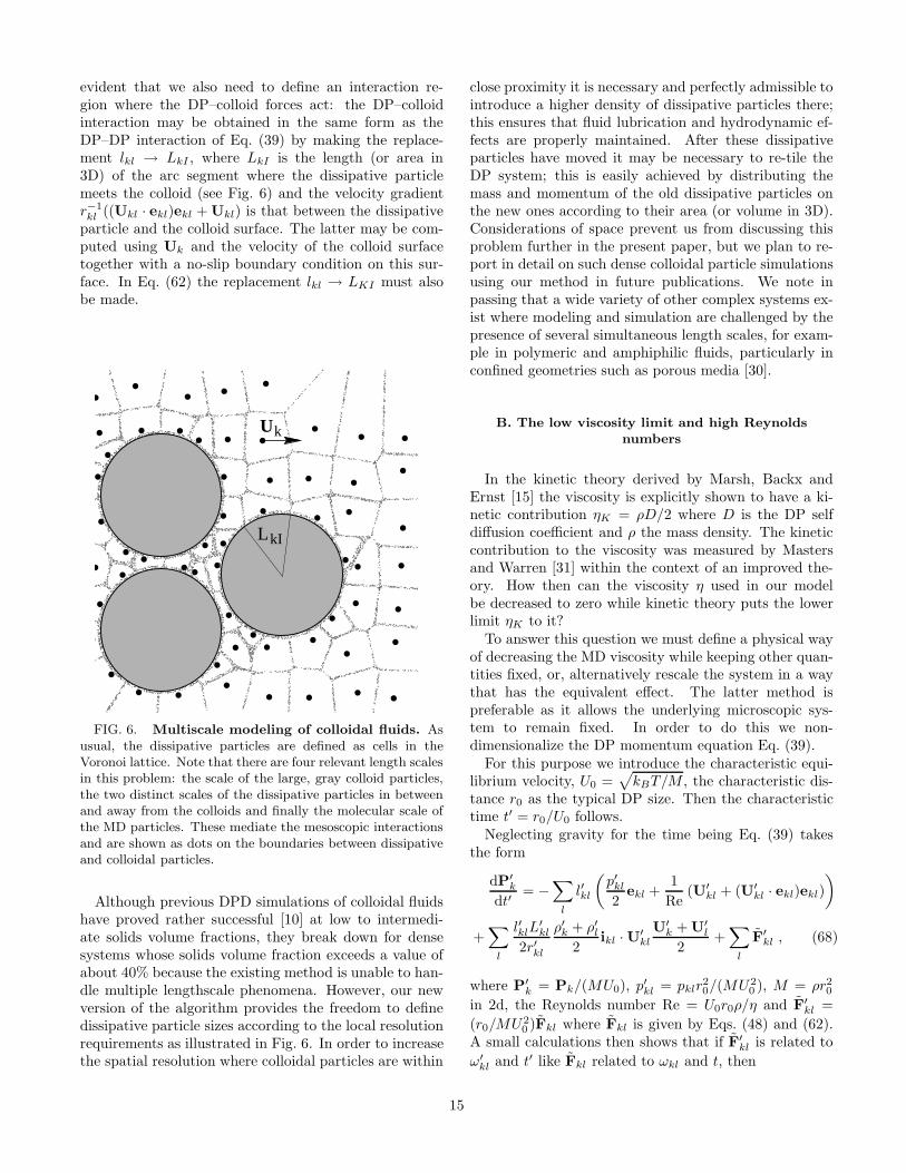
evident that we also need to define an interaction re-gion where the DP–colloid forces act: the DP–colloidinteraction may be obtained in the same form as theDP–DP interaction of Eq. (39) by making the replace-ment lkl → LkI , where LkI is the length (or area in3D) of the arc segment where the dissipative particlemeets the colloid (see Fig. 6) and the velocity gradientr−1kl ((Ukl · ekl)ekl + Ukl) is that between the dissipative

particle and the colloid surface. The latter may be com-puted using Uk and the velocity of the colloid surfacetogether with a no-slip boundary condition on this sur-face. In Eq. (62) the replacement lkl → LKI must alsobe made.

k

LkI

U

FIG. 6. Multiscale modeling of colloidal fluids. Asusual, the dissipative particles are defined as cells in theVoronoi lattice. Note that there are four relevant length scalesin this problem: the scale of the large, gray colloid particles,the two distinct scales of the dissipative particles in betweenand away from the colloids and finally the molecular scale ofthe MD particles. These mediate the mesoscopic interactionsand are shown as dots on the boundaries between dissipativeand colloidal particles.

Although previous DPD simulations of colloidal fluidshave proved rather successful [10] at low to intermedi-ate solids volume fractions, they break down for densesystems whose solids volume fraction exceeds a value ofabout 40% because the existing method is unable to han-dle multiple lengthscale phenomena. However, our newversion of the algorithm provides the freedom to definedissipative particle sizes according to the local resolutionrequirements as illustrated in Fig. 6. In order to increasethe spatial resolution where colloidal particles are within

close proximity it is necessary and perfectly admissible tointroduce a higher density of dissipative particles there;this ensures that fluid lubrication and hydrodynamic ef-fects are properly maintained. After these dissipativeparticles have moved it may be necessary to re-tile theDP system; this is easily achieved by distributing themass and momentum of the old dissipative particles onthe new ones according to their area (or volume in 3D).Considerations of space prevent us from discussing thisproblem further in the present paper, but we plan to re-port in detail on such dense colloidal particle simulationsusing our method in future publications. We note inpassing that a wide variety of other complex systems ex-ist where modeling and simulation are challenged by thepresence of several simultaneous length scales, for exam-ple in polymeric and amphiphilic fluids, particularly inconfined geometries such as porous media [30].

B. The low viscosity limit and high Reynolds

numbers

In the kinetic theory derived by Marsh, Backx andErnst [15] the viscosity is explicitly shown to have a ki-netic contribution ηK = ρD/2 where D is the DP selfdiffusion coefficient and ρ the mass density. The kineticcontribution to the viscosity was measured by Mastersand Warren [31] within the context of an improved the-ory. How then can the viscosity η used in our modelbe decreased to zero while kinetic theory puts the lowerlimit ηK to it?

To answer this question we must define a physical wayof decreasing the MD viscosity while keeping other quan-tities fixed, or, alternatively rescale the system in a waythat has the equivalent effect. The latter method ispreferable as it allows the underlying microscopic sys-tem to remain fixed. In order to do this we non-dimensionalize the DP momentum equation Eq. (39).

For this purpose we introduce the characteristic equi-librium velocity, U0 =

√

kBT/M , the characteristic dis-tance r0 as the typical DP size. Then the characteristictime t′ = r0/U0 follows.

Neglecting gravity for the time being Eq. (39) takesthe form

dP′k

dt′= −

∑

l

l′kl

(

p′kl

2ekl +

1

Re(U′

kl + (U′kl · ekl)ekl)

)

+∑

l

l′klL′kl

2r′kl

ρ′k + ρ′l2

ikl · U′kl

U′k + U′

l

2+∑

l

F′kl , (68)

where P′k = Pk/(MU0), p′kl = pklr

20/(MU2

0 ), M = ρr20

in 2d, the Reynolds number Re = U0r0ρ/η and F′kl =

(r0/MU20 )Fkl where Fkl is given by Eqs. (48) and (62).

A small calculations then shows that if F′kl is related to

ω′kl and t′ like Fkl related to ωkl and t, then

15

ω′2kl ≈

1

Re

kBT

MU20

≈ 1

Re(69)

where we have neglected dimensionless geometric prefac-tors like lkl/rkl and used the fact that the ratio of thethermal to kinetic energy by definition of U0 is one.

The above results imply that when the DPD system ismeasured in non-dimensionalized units everything is de-termined by the value of the mesoscopic Reynolds num-ber Re. There is thus no observable difference in thissystem between increasing r0 and decreasing η.

Returning to dimensional units again the DP diffusiv-ity may be obtained from the Stokes-Einstein relation[32] as

D =kBT

ar0η(70)

where a is some geometric factor (a = 6π for a sphere)and all quantities on the right hand side except r0 referdirectly to the underlying MD. As we are keeping theMD system fixed and increasing Re by increasing r0, itis seen that D and hence ηK vanish in the process.

We note in passing that if D is written in terms of themean free path λ: D = λ

√

kBT/(ρr20) and this result is

compared with Eq. (70) we get λ′ = λ/r0 ∼ 1/r0 in 2d,i.e. the mean free path, measured in units of the particlesize decreases as the inverse particle size. This is consis-tent with the decay of ηK . The above argument showsthat decreasing η is equivalent to keeping the microscopicMD system fixed while increasing the DP size, in whichcase the mean free path effects on viscosity is decreasedto zero as the DP size is increased to infinity. It is in thislimit that high Re values may be achieved.

Note that in this limit the thermal forces Fkl ∼ Re−1/2

will vanish, and that we are effectively left with a macro-scopic, fluctuationless description. This is no problemwhen using the present Voronoi construction. However,the effectively spherical particles of conventional DPDwill freeze into a colloidal crystal, i.e. into a lattice config-uration [8,9] in this limit. Also while conventional DPDhas usually required calibration simulations to determinethe viscosity, due to discrepancies between theory andmeasurements, the viscosity in this new form of DPD issimply an input parameter. However, there may still bediscrepancies due to the approximations made in goingfrom MD to DPD. These approximations include the lin-earization of the inter-DP velocity fields, the Markovianassumption in the force correlations and the neglect of aDP angular momentum variable.

None of the conclusions from the above argumentswould change if we had worked in three dimensions instead of two.

VII. CONCLUSIONS

We have introduced a systematic procedure for de-riving the mesoscopic modeling and simulation methodknown as dissipative particle dynamics from the under-lying description in terms of molecular dynamics.

Fokker-Planck equations

DPD2: Langevin equations

DPD1

Time symmetric

coarsed grained equations

of motion

MD

ω= ω(η T, )

equilibrium statistical mechanics

constitutive relations and Markovian assumption

averaging over MD configurations

coarse graining

Fluctuation dissipation

DPD complete

Fluctuating

hydrodynamics

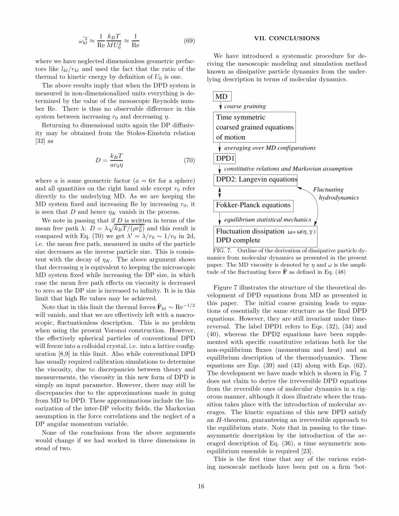
FIG. 7. Outline of the derivation of dissipative particle dy-namics from molecular dynamics as presented in the presentpaper. The MD viscosity is denoted by η and ω is the ampli-tude of the fluctuating force F as defined in Eq. (48)

Figure 7 illustrates the structure of the theoretical de-velopment of DPD equations from MD as presented inthis paper. The initial coarse graining leads to equa-tions of essentially the same structure as the final DPDequations. However, they are still invariant under time-reversal. The label DPD1 refers to Eqs. (32), (34) and(40), whereas the DPD2 equations have been supple-mented with specific constitutive relations both for thenon-equilibrium fluxes (momentum and heat) and anequilibrium description of the thermodynamics. Theseequations are Eqs. (39) and (43) along with Eqs. (62).The development we have made which is shown in Fig. 7does not claim to derive the irreversible DPD equationsfrom the reversible ones of molecular dynamics in a rig-orous manner, although it does illustrate where the tran-sition takes place with the introduction of molecular av-erages. The kinetic equations of this new DPD satisfyan H-theorem, guaranteeing an irreversible approach tothe equilibrium state. Note that in passing to the time-asymmetric description by the introduction of the av-eraged description of Eq. (36), a time asymmetric non-equilibrium ensemble is required [23].

This is the first time that any of the various exist-ing mesoscale methods have been put on a firm ‘bot-

16

tom up’ theoretical foundation, a development whichbrings with it numerous new insights as well as prac-tical advantages. One of the main virtues of this proce-dure is the capability it provides to choose one or morecoarse-graining lengthscales to suit the particular model-ing problem at hand. The relative scale between molecu-lar dynamics and the chosen dissipative particle dynam-ics, which may be defined as the ratio of their numberdensities ρDPD/ρMD, is a free parameter within the the-ory. Indeed, this rescaling may be viewed as a renormal-isation group procedure under which the fluid viscosityremains constant: since the conservation laws hold ex-actly at every level of coarse graining, the result of doingtwo rescalings, say from MD to DPDα and from DPDαto DPDβ, is the same as doing just one with a largerratio, i.e. ρDPDβ/ρMD = (ρDPDβ/ρDPDα)(ρDPDα/ρMD).

The present coarse graining scheme is not limited tohydrodynamics. It could in principle be used to rescalethe local description of any quantity of interest. However,only for locally conserved quantities will the DP particleinteractions take the form of surface terms as here, andso it is unlikely that the scheme will produce a usefuldescription of non-conserved quantities.

In this context, we note that the bottom-up approachto fluid mechanics presented here may throw new lighton aspects of the problem of homogeneous and inhomo-geneous turbulence. Top-down multiscale methods and,to a more limited extent, ideas taken from renormali-sation group theory have been applied quite widely inrecent years to provide insight into the nature of turbu-lence [33,34]; one might expect an alternative perspectiveto emerge from a fluid dynamical theory originating atthe microscopic level, in which the central relationshipbetween conservative and dissipative processes is speci-fied in a more fundamental manner. From a practicalpoint of view it is noted that, since the DPD viscosity isthe same as the viscosity emergent from the underlyingMD level, it may be treated as a free parameter in theDPD model, and thus high Reynolds numbers may bereached. In the η → 0 limit the model thus representsa potential tool for hydrodynamic simulations of turbu-lence. However, we have not investigated the potentialnumerical complications of this limit.

The dissipative particle dynamics which we have de-rived is formally similar to the conventional version, in-corporating as it does conservative, dissipative and fluc-tuating forces. The interactions are pairwise, and con-serve mass and momentum as well as energy. However,now all these forces have been derived from the under-lying molecular dynamics. The conservative and dissi-pative forces arise directly from the hydrodynamic de-scription of the molecular dynamics and the properties ofthe fluctuating forces are determined via a fluctuation–dissipation relation.

The simple hydrodynamic description of the moleculeschosen here is not a necessary requirement. Other choices

for the average of the general momentum and energy fluxtensors Eqs. (26) and (19) may be made and we hopethese will be explored in future work. More significantis the fact that our analysis permits the introduction ofspecific physicochemical interactions at the mesoscopiclevel, together with a well-defined scale for this meso-scopic description.

While the Gaussian basis we used for the samplingfunctions is an arbitrary albeit convenient choice, theVoronoi geometry itself emerged naturally from the re-quirement that all the MD particles be fully accountedfor. Well defined procedures already exist in the litera-ture for the computation of Voronoi tesselations [35] andso algorithms based on our model are not computation-ally difficult to implement. Nevertheless, it should be ap-preciated that the Voronoi construction represents a sig-nificant computational overhead. This overhead is of or-der N log N , a factor log N larger than the most efficientmultipole methods in principle available for handling theparticle interactions in molecular dynamics. However,the prefactors are likely to be much larger in the particleinteraction case.

Finally we note the formal similarity of the present par-ticulate description to existing continuum fluid dynam-ics methods incorporating adaptive meshes, which startout from a top-down or macroscopic description. Thesetop-down approaches include in particular smoothed par-ticle hydrodynamics [19] and finite-element simulations.In these descriptions too the computational method isbased on tracing the motion of elements of the fluid onthe basis of the forces acting between them [36]. However,while such top-down computational strategies depend ona macroscopic and purely phenomenological fluid descrip-tion, the present approach rests on a molecular basis.

ACKNOWLEDGMENTS

It is a pleasure to thank Frank Alexander, BruceBoghosian and Jens Feder for many helpful and stim-ulating discussions. We are grateful to the Departmentof Physics at the University of Oslo and SchlumbergerCambridge Research for financial support which enabledPVC to make several visits to Norway in the course of1998; and to NATO and the Centre for ComputationalScience at Queen Mary and Westfield College for fundingvisits by EGF to London in 1999 and 2000.

[1] L. D. Landau and E. M. Lifshitz, Fluid Mechanics (Perg-amon Press, New York, 1959).

17

[2] L. Boltzmann., Vorlesungen uber Gastheorie (Leipzig,1872).

[3] J. Koplik and J. R. Banavar, Ann. Rev. Fluid Mech. 27,257 (1995).

[4] U. Frisch, B. Hasslacher, and Y. Pomeau, Phys. Rev.Lett. 56, 1505 (1986).

[5] G. McNamara and G. Zanetti, Phys. Rev. Lett. 61, 2332(1988).

[6] X. W. Chan and H. Chen, Phys. Rev E 49, 2941 (1993).[7] M. R. Swift, W. R. Osborne, and J. Yeomans, Phys. Rev.

Lett. 75, 830 (1995).[8] P. J. Hoogerbrugge and J. M. V. A. Koelman, Europhys.

Lett. 19, 155 (1992).[9] P. Espanol and P. Warren, Europhys. Lett. 30, 191

(1995).[10] E. S. Boek, P. V. Coveney, H. N. W. Lekkerkerker, and

P. van der Schoot, Phys. Rev. E 54, 5143 (1997).[11] A. G. Schlijper, P. J. Hoogerbrugge, and C. W. Manke,

J. Rheol. 39, 567 (1995).[12] P. V. Coveney and K. E. Novik, Phys. Rev. E 54, 5143

(1996).[13] R. D. Groot and P. B. Warren., J. Chem. Phys. 107,

4423 (1997).[14] P. Espanol, Phys. Rev. E 52, 1734 (1995).[15] C. A. Marsh, G. Backx, and M. Ernst, Phys. Rev. E 56,

1676 (1997).[16] J. B. Avalos and A. D. Mackie, Europhys. Lett. 40, 141

(1997).[17] P. Espanol, Europhys. Lett 40, 631 (1997).[18] P. Espanol, Phys. Rev. E 57, 2930 (1998).[19] J. J. Monaghan, Ann. Rev. Astron. Astophys. 30, 543

(1992).[20] P. Espanol, M. Serrano, and I. Zuniga, Int. J. Mod. Phys.

C 8, 899 (1997).

[21] E. G. Flekkøy and P. V. Coveney, Phys. Rev. Lett. 83,1775 (1999).

[22] P. V. Coveney and O. Penrose, J. Phys A: Math. Gen.25, 4947 (1992).

[23] O. Penrose and P. V. Coveney, Proc. R. Soc. 447, 631(1994).

[24] P. V. Coveney and R. Highfield, The Arrow of Time(W. H.Allen, London, 1990).

[25] C. A. Marsh and P. V. Coveney, J. Phys. A: Math. Gen.31, 6561 (1998).

[26] F. Reif, Fundamentals of statistical and thermal physics(Mc Graw-Hill, Singapore, 1965).

[27] L. D. Landau and E. M. Lifshitz, Statistical Physics(Pergamon Press, New York, 1959).

[28] C. W. Gardiner, Handbook of stochastic methods(Springer Verlag, Berlin Heidelberg, 1985).

[29] G. D. Fabritiis, P. V. Coveney, and E. G. Flekkøy, inProc. 5th European SGI/Cray MPP Workshop, Bologna,Italy 1999.

[30] P. V. Coveney, J. B. Maillet, J. L. Wilson, P. W. Fowler,O. Al-Mushadani and B. M. Boghosian, Int. J. Mod.Phys. C 9, 1479 (1998).

[31] A. J. Masters and P. B. Warren, preprint cond-mat/9903293 (http://xxx.lanl.gov/) (unpublished).

[32] A. Einstein, Ann. Phys. 17, 549 (1905).[33] U. Frisch, Turbulence (Cambridge University Press,

Cambridge, 1995).[34] A. Bensoussan, J. L. Lions, and G. Papanicolaou, Asymp-

totic Analysis for Periodic Structures (North-Holland,Amsterdam, 1978).

[35] D. E. K. L. J. Guibas and M. Sharir, Algorithmica 7, 381(1992).

[36] B. M. Boghosian, Encyclopedia of Applied Physics 23,151 (1998).

18