A dissipative particle dynamics method for arbitrarily complexgeometries

Zhen Li∗, Xin Bian, Yu-Hang Tang and George Em Karniadakis†

Division of Applied Mathematics, Brown University, Providence, Rhode Island, 02912, USA

December 30, 2016

Abstract

Dissipative particle dynamics (DPD) is an effective Lagrangian method for modeling complexfluids in the mesoscale regime but so far it has been limited to relatively simple geometries. Here,we formulate a local detection method for DPD involving arbitrarily shaped geometric three-dimensional domains. By introducing an indicator variable of boundary volume fraction (BVF)for each fluid particle, the boundary of arbitrary-shape objects is detected on-the-fly for the mov-ing fluid particles using only the local particle configuration. Therefore, this approach eliminatesthe need of an analytical description of the boundary and geometry of objects in DPD simula-tions and makes it possible to load the geometry of a system directly from experimental imagesor computer-aided designs/drawings. More specifically, the BVF of a fluid particle is defined bythe weighted summation over its neighboring particles within a cutoff distance. Wall penetrationis inferred from the value of the BVF and prevented by a predictor-corrector algorithm. The no-slip boundary condition is achieved by employing effective dissipative coefficients for liquid-solidinteractions. Quantitative evaluations of the new method are performed for the plane Poiseuilleflow, the plane Couette flow and the Wannier flow in a cylindrical domain and compared with theircorresponding analytical solutions and (high-order) spectral element solution of the Navier-Stokesequations. We verify that the proposed method yields correct no-slip boundary conditions for ve-locity and generates negligible fluctuations of density and temperature in the vicinity of the wallsurface. Moreover, we construct a very complex 3D geometry – the “Brown Pacman” microfluidicdevice – to explicitly demonstrate how to construct a DPD system with complex geometry directlyfrom loading a graphical image. Subsequently, we simulate the flow of a surfactant solution throughthis complex microfluidic device using the new method. Its effectiveness is demonstrated by exam-ining the rich dynamics of surfactant micelles, which are flowing around multiple small cylindersand stenotic regions in the microfluidic device without wall penetration. In addition to stationaryarbitrary-shape objects, the new method is particularly useful for problems involving moving anddeformable boundaries, because it only uses local information of neighboring particles and satisfiesthe desired boundary conditions on-the-fly.

1 Introduction

Despite of the sustained fast growth of computing power during the past few decades, it is still compu-tationally prohibitive or impractical to model long time scales and large spatial scales in many appli-

∗Email: zhen li@brown.edu†Email: george karniadakis@brown.edu

1

arX

iv:1

612.

0876

1v1

[ph

ysic

s.co

mp-

ph]

27

Dec

201

6

cations of soft matter and biological systems with the brute-force atomistic simulations [1, 2]. If onlythe mesoscopic properties and collective behavior are of practical interest, it may not be necessary toexplicitly take into account all the details of materials at the atomic/molecular level [3]. To this end, acoarse-graining approach eliminates fast degrees of freedom and drastically simplifies the dynamics onatomistic scales, while providing a cost-effective simulation path to capturing the correct properties ofcomplex fluids at larger spatial and temporal scales beyond the capacity of conventional atomistic sim-ulations [4]. In recent years, with increasing attention on the research of soft matter and biophysics [5],coarse-grained (CG) modeling has become a rapidly expanding methodology especially in the simula-tions of polymers [6, 7, 8], colloidal suspensions [9, 10, 11], interfaces of multiphase fluids [12, 13, 14],cell dynamics [15, 16, 17], blood rheology [18, 19, 20] and biological materials [21, 22, 23].

Initially proposed by Hoogerbrugge and Koelman [24], dissipative particle dynamics (DPD) is oneof the currently most popular CG methods [25, 26] for performing mesoscopic simulations of complexfluids. The DPD particles are defined as coarse-grained entities [27, 28], which represent clusters ofmolecules rather than atoms/molecules directly. In contrast to molecular dynamics (MD) method,DPD allows much larger particle size and also time steps because of the soft particle interactions. As aparticle-based mesoscopic method, DPD considers N particles, whose state variables of momentum andposition are governed by the Newton’s equations of motion [29]. For a typical DPD particle i, its timeevolution follows ri = vi and pi = Fi =

∑i 6=j(F

Cij + FD

ij + FRij) where ri, vi, pi and Fi denote position,

velocity, momentum and force vectors, respectively. The summation for computing the total force Fi

is carried out over all other particles within a cutoff radius rc beyond which the forces are considerednegligible. The pairwise force Fij comprises conservative (FC

ij), dissipative (FDij ) and random (FR

ij) forcesare expressed as [29]

FCij = aijωC(rij)eij,

FDij = −γijωD(rij)(eij · vij)eij,

FRij = σijωR(rij)dWijeij,

(1)

where rij = |rij| = |ri−rj| represents the distance between two particles i and j, eij = rij/rij is the unitvector from particles j to i, and vij = vi−vj is the velocity difference; dWij is an independent incrementof the Wiener process [30]. Also, γij is the dissipative coefficient and σij sets the strength of random force.The dissipative force and random force together act as a thermostat when the dissipative coefficient γand the amplitudes of white noise σ satisfy the fluctuation-dissipation theorem (FDT) [31, 30] requiringσ2 = 2γkBT and ωD(r) = ω2

R(r). All these forces in Eq. (1) have the same finite interaction range rc andtheir amplitudes decay according to corresponding weight functions. A common choice of the weightfunctions [29] is ωC(r) = 1− r/rc and ωD(r) = ω2

R(r) = (1− r/rc)2 for r ≤ rc and zero for r > rc.All the three forces between DPD particles are soft and short-range interactions, which allows large

time steps for the time integration of the particle-based system. The soft interactions between DPDparticles, unlike the hard potentials in atomistic simulations, cannot prevent fluid particles from pene-trating wall boundaries [32]. It is also unlike the top-down smoothed particle hydrodynamics (SPH) [33]or smoothed DPD (SDPD) [9] approach, where the equation of state can be tuned so that the pressureis arbitrarily strong to prevent particle penetration. As a result, for wall-bounded flow systems, DPDsimulations require extra formulations [34, 35, 36] to prevent the penetration of the liquid particles intosolid boundaries. Specular, Maxwellian, and bounce-back reflections [37] are common techniques usedto reflect particles back into the fluid after they cross the wall surface. Therefore, for wall-boundedflows one has to mathematically predefine the position of solid wall to judge the penetration of fluidparticles before a DPD simulation can be performed, which is difficult to extend for arbitrarily shapedboundaries and limits the applicability of DPD.

2

In the present paper, we develop a boundary method for imposing correctly the no-slip bound-ary condition on the solid walls with arbitrary shapes. Instead of predefining the position of the wallboundary, we make the fluid particles autonomous to detect the wall surface and to infer the wallpenetration by themselves based on the local information of their neighboring particles. Hence, thegeometry of solid boundary can be computed on-the-fly using local particle configurations. Therefore,it is no longer necessary to predefine the boundary geometry for DPD simulations, which makes itpossible to construct DPD systems with arbitrary-shape domains directly from loading experimentalimages or computer-aided designs/drawings. Furthermore, since this boundary method uses local infor-mation of neighboring particles and satisfies no-slip/partial-slip boundary conditions on-the-fly, it is notonly valuable for stationary arbitrary-shape boundaries but also for moving boundaries and deformableboundaries.

The remainder of this paper is organized as follows: Section 2 introduces the details of the boundarymethod, and also how to compute the effective dissipative coefficient for liquid-solid interactions. InSection 3, we validate the proposed boundary method by performing the Poiseuille flow, the Couetteflow and the Wannier flow with comparison to analytical solutions. Moreover, an error analysis of thisboundary method related to the curvature of arbitrary-shaped boundaries is provided in Appendix A.We also include a demonstration of micelles flowing through a very complex microfludic device. Finally,we end with a brief summary and discussion in Section 4.

2 Wall Boundary Method

2.1 Definition of the boundary volume fraction

Consider a fluid particle i in the vicinity of a solid wall represented by discrete DPD particles and weassign to it an extra variable φi = ϕ(ri) in addition to other quantities such as position and momentum.We define φi as the boundary volume fraction (BVF) depending on the coordinates of particle i. Morespecifically, the value of φi is computed using a weighted summation over neighboring solid particles jgiven by

φi = ϕ(ri) =1

ρw

j∈S∑rij<rcw

W (rij, rcw) , (2)

where W (r, rcw) is a weighting function, and ρw is the bulk number density of solid particles. Theweighting function W (r, rcw) can be any smoothing kernel, such as the ones used widely in smoothedparticle hydrodynamics [38, 39]. As a demonstration, we choose the three-dimensional Lucy kernel [40]

W (r, rcw) =105

16πr3cw

(1 +

3r

rcw

)(1− r

rcw

)3

, (3)

where r is the norm of r, and rcw is the cutoff radius beyond which W (r, rcw) is considered zero. Largerrcw increases the computational cost but yields smoother ϕ(r), as we will discuss in section 3. Unlessotherwise specified, in testing cases we simply set rcw equal to rc.

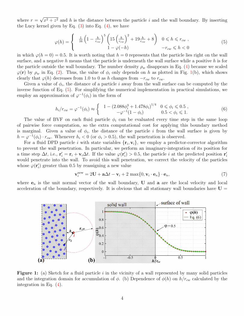
Consider a planar wall surface or a wall surface with a radius of curvature far greater than the cutoffradius rcw, as shown in Fig. 1(a); we estimate the value of φi using the continuum approximation

φi = ϕ(h) =

∫ rcw

z=h

∫ √rcw2−z2

x=0

2πxW (r, rcw) · dx · dz (4)

3

where r =√x2 + z2 and h is the distance between the particle i and the wall boundary. By inserting

the Lucy kernel given by Eq. (3) into Eq. (4), we have

ϕ(h) =

116

(1− h

rcw

)5(

15(

hrcw

)2

+ 19 hrcw

+ 8

)0 6 h 6 rcw ,

1− ϕ(−h) −rcw 6 h < 0(5)

in which ϕ(h = 0) = 0.5. It is worth noting that h = 0 represents that the particle lies right on the wallsurface, and a negative h means that the particle is underneath the wall surface while a positive h is forthe particle outside the wall boundary. The number density ρw disappears in Eq. (4) because we scaledϕ(r) by ρw in Eq. (2). Thus, the value of φi only depends on h as plotted in Fig. 1(b), which showsclearly that ϕ(h) decreases from 1.0 to 0 as h changes from −rcw to rcw.

Given a value of φi, the distance of a particle i away from the wall surface can be computed by theinverse function of Eq. (5). For simplifying the numerical implementation in practical simulations, weemploy an approximation of ϕ−1(φi) in the form of

hi/rcw = ϕ−1(φi) ≈

1− (2.088φ3i + 1.478φi)

1/40 6 φi 6 0.5 ,

−ϕ−1(1− φi) 0.5 < φi 6 1.(6)

The value of BVF on each fluid particle φi can be evaluated every time step in the same loopof pairwise force computation, so the extra computational cost for applying this boundary methodis marginal. Given a value of φi, the distance of the particle i from the wall surface is given byh = ϕ−1(φi) · rcw. Whenever hi < 0 (or φi > 0.5), the wall penetration is observed.

For a fluid DPD particle i with state variables ri,vi, we employ a predictor-corrector algorithmto prevent the wall penetration. In particular, we perform an imaginary-integration of its position fora time step ∆t, i.e., r′i = ri + vi∆t. If the value ϕ(r′i) > 0.5, the particle i at the predicted position r′iwould penetrate into the wall. To avoid this wall penetration, we correct the velocity of the particleswhose ϕ(r′i) greater than 0.5 by reassigning a new value

vnewi = 2U + a∆t− vi + 2 max0,vi · en · en, (7)

where en is the unit normal vector of the wall boundary, U and a are the local velocity and localacceleration of the boundary, respectively. It is obvious that all stationary wall boundaries have U =

Figure 1: (a) Sketch for a fluid particle i in the vicinity of a wall represented by many solid particlesand the integration domain for accumulation of φ. (b) Dependence of φ(h) on h/rcw calculated by theintegration in Eq. (4).

4

a = 0. For moving boundaries, the value of U and a can take the values of velocity and acceleration ofthe nearest wall particle in practical DPD simulations. Let nw be the gradient of ϕ(ri) at the locationof particle i, which is computed by

nw = ∇ϕ(ri) =1

ρw

j∈S∑rij<rcw

rijrij

dW (rij, rcw)

drij. (8)

Then, the unit normal vector of the wall boundary en = nw/nw where nw is the modulus of nw.

2.2 Control of the surface roughness

Consider a flat wall represented by solid particles in uniform lattices, the iso-surface of φ = 0.5 issmooth and flat, which can accurately represent the surface of the flat wall. However, the structure ofsolid particles associated with these lattices will induce unwanted fluctuations [34] of fluid density andtemperature in the vicinity of wall boundary. In the present paper, we employ randomly distributedparticles in the wall domain to represent the wall boundary, which is easier and more general forconstruction of fluid system with complex geometry and arbitrarily shaped boundaries.

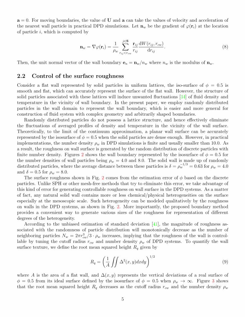
Randomly distributed particles do not possess a lattice structure, and hence effectively eliminatethe fluctuations of averaged profiles of density and temperature in the vicinity of the wall surface.Theoretically, to the limit of the continuum approximation, a planar wall surface can be accuratelyrepresented by the isosurface of φ = 0.5 when the solid particles are dense enough. However, in practicalimplementations, the number density ρw in DPD simulations is finite and usually smaller than 10.0. Asa result, the roughness on wall surface is generated by the random distribution of discrete particles withfinite number density. Figures 2 shows the wall boundary represented by the isosurface of φ = 0.5 forthe number densities of wall particles being ρw = 4.0 and 8.0. The solid wall is made up of randomlydistributed particles, where the average distance between these particles is δ = ρ

−1/3w = 0.63 for ρw = 4.0

and δ = 0.5 for ρw = 8.0.The surface roughness shown in Fig. 2 comes from the estimation error of φ based on the discrete

particles. Unlike SPH or other mesh-free methods that try to eliminate this error, we take advantage ofthis kind of error for generating controllable roughness on wall surface in the DPD systems. As a matterof fact, any natural solid wall contains more or less chemical/physical heterogeneities on the surfaceespecially at the mesoscopic scale. Such heterogeneity can be modeled qualitatively by the roughnesson walls in the DPD systems, as shown in Fig. 2. More importantly, the proposed boundary methodprovides a convenient way to generate various sizes of the roughness for representation of differentdegrees of the heterogeneity.

According to the unbiased estimation of standard deviation [41], the magnitude of roughness as-sociated with the randomness of particle distribution will monotonically decrease as the number ofneighboring particles Nw = 2πr3

cw/3 · ρw increases, implying that the roughness of the wall is control-lable by tuning the cutoff radius rcw and number density ρw of DPD systems. To quantify the wallsurface texture, we define the root mean squared height Rq given by

Rq =

(1

A

∫∫∆2(x, y)dxdy

)1/2

(9)

where A is the area of a flat wall, and ∆(x, y) represents the vertical deviations of a real surface ofφ = 0.5 from its ideal surface defined by the isosurface of φ = 0.5 when ρw → ∞. Figure 3 showsthat the root mean squared height Rq decreases as the cutoff radius rcw and the number density ρw

5

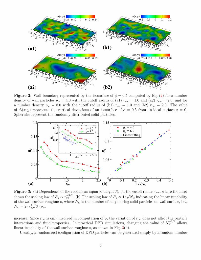
Figure 2: Wall boundary represented by the isosurface of φ = 0.5 computed by Eq. (2) for a numberdensity of wall particles ρw = 4.0 with the cutoff radius of (a1) rcw = 1.0 and (a2) rcw = 2.0, and fora number density ρw = 8.0 with the cutoff radius of (b1) rcw = 1.0 and (b2) rcw = 2.0. The valueof ∆(x, y) represents the vertical deviations of an isosurface of φ = 0.5 from its ideal surface z = 0.Spherules represent the randomly distributed solid particles.

Figure 3: (a) Dependence of the root mean squared height Rq on the cutoff radius rcw, where the inset

shows the scaling law of Rq ∼ r−3/2cw . (b) The scaling law of Rq ∝ 1/

√Nw indicating the linear tunability

of the wall surface roughness, where Nw is the number of neighboring solid particles on wall surface, i.e.,Nw = 2πr3

cw/3 · ρw.

increase. Since rcw is only involved in computation of φ, the variation of rcw does not affect the particleinteractions and fluid properties. In practical DPD simulations, changing the value of N

−1/2w allows

linear tunability of the wall surface roughness, as shown in Fig. 3(b).Usually, a randomized configuration of DPD particles can be generated simply by a random number

6

generator, which may result in overlapping of particles or large vacancies in wall boundaries. To avoidthe overlaps or vacancies, a more uniform particle distribution is needed, which can be achieved by aprocess of geometry optimization or a short run of particle-based simulation. In the present paper, wecarry out a short DPD simulation with a relatively large conservative force coefficient to get the initialparticle positions. Then, the particles in the wall domain are frozen as solid particles, while others inthe fluid domain are taken as the fluid particles. For instance, the wall boundary shown in Fig. 2 isobtained by running 1000 time steps of DPD simulation from totally randomized particles.

2.3 Effective dissipative interaction

The dissipative force between two DPD particles is computed by FDIJ = −γ · ωD(rij)(eij · vij)eij, where

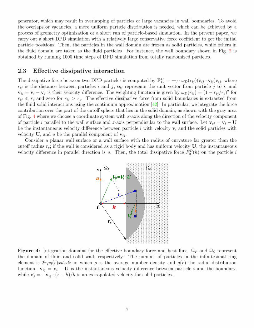
rij is the distance between particles i and j, eij represents the unit vector from particle j to i, andvij = vi − vj is their velocity difference. The weighting function is given by ωD(rij) = (1− rij/rc)2 forrij 6 rc and zero for rij > rc. The effective dissipative force from solid boundaries is extracted fromthe fluid-solid interactions using the continuum approximation [42]. In particular, we integrate the forcecontribution over the part of the cutoff sphere that lies in the solid domain, as shown with the gray areaof Fig. 4 where we choose a coordinate system with x-axis along the direction of the velocity componentof particle i parallel to the wall surface and z-axis perpendicular to the wall surface. Let vij = vi −Ube the instantaneous velocity difference between particle i with velocity vi and the solid particles withvelocity U, and u be the parallel component of vij.

Consider a planar wall surface or a wall surface with the radius of curvature far greater than thecutoff radius rc; if the wall is considered as a rigid body and has uniform velocity U, the instantaneousvelocity difference in parallel direction is u. Then, the total dissipative force FD

0 (h) on the particle i

Figure 4: Integration domains for the effective boundary force and heat flux. ΩF and ΩS representthe domain of fluid and solid wall, respectively. The number of particles in the infinitesimal ringelement is 2πρg(r)xdxdz in which ρ is the average number density and g(r) the radial distributionfunction. vij = vi − U is the instantaneous velocity difference between particle i and the boundary,while v′j = −vij · (z − h)/h is an extrapolated velocity for solid particles.

7

due to the presence of wall boundary can be evaluated by:

FD0 (h) =

∫ rC

z=h

∫ √rC2−z2

x=0

∫ 2π

θ=0

(−γ · ωD(rij)(eij · vij)eij · ρ · g(r) · dx · x · dθ · dz)

=

∫ rC

z=h

∫ √rC2−z2

x=0

(−γπρ · u ·

(1− r

rc

)2

· x3

r2· g(r) · dx · dz

)g(r)=1

===== −γπρur3c

[1

45− 1

12

h

rc−(h

rc

)3(1

3log

(h

rc

)+

2

9

)+

1

3

(h

rc

)4

− 1

20

(h

rc

)5]

(10)

However, the value of FD0 (h) is not sufficient to impose the correct no-slip boundary condition on the

wall surface. To this end, we assign an extrapolated velocity v′j = −vij · (z− h)/h to each solid particleso that the wall surface has zero velocity, and hence the instantaneous velocity difference becomesvij = vij − v′j = vij · z/h, in which the parallel component is u · z/h. Then, the corrected dissipativeforce FD

cor(h) on the particle i due to the presence of wall boundary is computed by:

FDcor(h) =

∫ rC

z=h

∫ √rC2−z2

x=0

∫ 2π

θ=0

(−γ · ωD(rij)(eij · vij)eij · ρ · g(r) · dx · x · dθ · dz)

=

∫ rC

z=h

∫ √rC2−z2

x=0

(−γπρ ·

(zhu)·(

1− r

rc

)2

· x3

r2· g(r) · dx · dz

)g(r)=1

===== −γπρur3c

[1

240

rch− 1

24

h

rc− 1

4

(h

rc

)3 [log

(h

c

)+

3

4

]+

4

15

(h

rc

)4

− 1

24

(h

rc

)5](11)

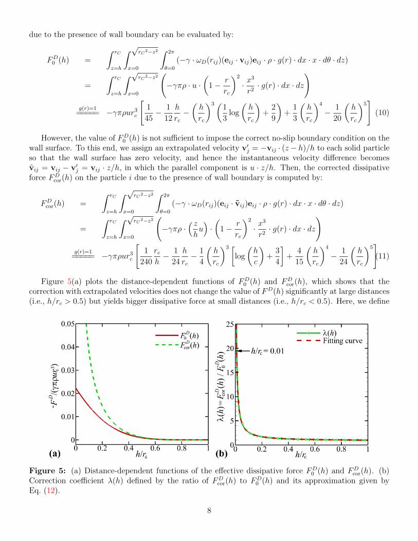
Figure 5(a) plots the distance-dependent functions of FD0 (h) and FD

cor(h), which shows that thecorrection with extrapolated velocities does not change the value of FD(h) significantly at large distances(i.e., h/rc > 0.5) but yields bigger dissipative force at small distances (i.e., h/rc < 0.5). Here, we define

Figure 5: (a) Distance-dependent functions of the effective dissipative force FD0 (h) and FD

cor(h). (b)Correction coefficient λ(h) defined by the ratio of FD

cor(h) to FD0 (h) and its approximation given by

Eq. (12).

8

the ratio of FDcor(h) to FD

0 (h) as a correction coefficient λ(h) = FDcor(h)/FD

0 (h), which is plotted inFig. 5(b). In practical implementation, the distance-dependent coefficient λ(h) can be approximated by

λ(h) = λ(ϕ−1(φ) · rcw) ≈

1 + 0.187

(rch− 1)− 0.093

(1− h

rc

)3

0.01 6 h/rc 6 1.0 ,

19.423 h/rc < 0.01 .(12)

Let the effective dissipative coefficient for liquid-solid interaction be γe = λ(h) · γ. We note that theformula of Eq. (12) is obtained based on g(r) = 1. A more accurate function of λ(h) can be derived fromEqs. (10) and (11) using the computed g(r). For easier numerical implementation using Eq. (12) directlywithout computation of g(r), it is recommended to keepNw = 2πr3

cw/3·ρw > 15, i.e., setting rcw > 1.35 atρw = 3 and rcw > 1.0 at ρw = 8, so that the value of φ can be evaluated accurately. Then, the dissipativeforce between liquid particles and solid particles is computed by FD

IJ = −γe · ωD(rij)(eij · vij)eij, whichguarantees the no-slip boundary condition at the wall surface. The corresponding random force is givenby FR

IJ = σe · ωR(rij)dW ijeij with σe = 2kBTγe and dWij being independent increments of the Wienerprocess to satisfy the FDT [30]. In the next section, we will verify the validity and the accuracy of theboundary method using the effective dissipative coefficient for liquid-solid interaction.

3 Numerical Results

In this section, we examine the accuracy of the proposed boundary method for well-known flows such asthe plane Poiseuille flow, the plane Couette flow and the Wannier cylindrical flow. Then, a demonstrationof flow in a “Brown Pacman” microfluidic device involving very complex boundaries is performed.

Firstly, we test the accuracy of the boundary method on stationary walls by carrying out a DPDsimulation of the plane Poiseuille flow, in which a body force field acting in the x-direction on a fluidbetween two flat plates in the xy-plane. In this simple case, the Navier-Stokes equations admit the exactsolution of the velocity profile given by [43]

u(z, t) =Fd2

8υ

(1−

(2z

d

)2)−∞∑n=0

4(−1)nFd2

υπ3(2n+ 1)3 · cos

[(2n+ 1) πz

d

]· exp

[−(2n+ 1)2π2υt

d2

], (13)

where d is the separation of the plates, υ the kinematic viscosity and F a driving force per unit mass.The parameter set for the Poiseuille flow is ρ = 8.0, kBT = 1.0, a = 75.0kBT/ρ, γ = 4.5, σ = 3.0and rc = rcw = 1.0. The kinematic viscosity of the DPD fluid can be computed by running a periodicPoiseuille flow [44], which gives υ = 0.275.

More specifically, the DPD simulation of transient Poiseuille flow is performed in a computationaldomain of 30.0× 5.0× 24.0 in DPD units, which contains 24000 fluid particles and 4800 frozen particlesfor solid walls with a thickness of 2.0. The system is initialized with stationary fluid and two stationarywalls. Periodic boundary condition is applied in x- and y-directions and no-slip boundary condition inz-direction. Then, a body force gx = 0.02 is applied on each DPD particle to drive the fluid, which isequivalent to imposing a pressure drop of ρgxLx on the channel of length Lx. To extract the velocityprofile from the DPD simulation, we divide the computational domain into 48 bins of width ∆ = 0.5along the z-direction. The transient velocity profiles at t = 10, 50, 100, 200 and at steady state areplotted in Fig. 6(a), where all local flow properties including particle density and kinetic temperature areobtained by averaging enough sampled data from 100 independent simulations initialized with differentrandom seeds. The first and last bins contain both fluid and solid volumes because of the roughness ofthe wall surface, as shown in Fig. 2. Considering the flat solid walls are made of randomly distributedparticles, the volume of the raised part equals to the volume of the sunk part on average. Therefore,

9

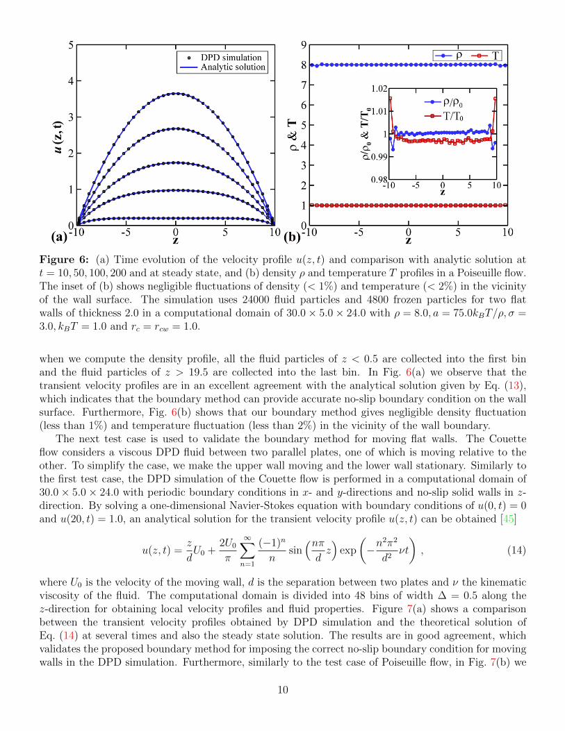
Figure 6: (a) Time evolution of the velocity profile u(z, t) and comparison with analytic solution att = 10, 50, 100, 200 and at steady state, and (b) density ρ and temperature T profiles in a Poiseuille flow.The inset of (b) shows negligible fluctuations of density (< 1%) and temperature (< 2%) in the vicinityof the wall surface. The simulation uses 24000 fluid particles and 4800 frozen particles for two flatwalls of thickness 2.0 in a computational domain of 30.0× 5.0× 24.0 with ρ = 8.0, a = 75.0kBT/ρ, σ =3.0, kBT = 1.0 and rc = rcw = 1.0.

when we compute the density profile, all the fluid particles of z < 0.5 are collected into the first binand the fluid particles of z > 19.5 are collected into the last bin. In Fig. 6(a) we observe that thetransient velocity profiles are in an excellent agreement with the analytical solution given by Eq. (13),which indicates that the boundary method can provide accurate no-slip boundary condition on the wallsurface. Furthermore, Fig. 6(b) shows that our boundary method gives negligible density fluctuation(less than 1%) and temperature fluctuation (less than 2%) in the vicinity of the wall boundary.

The next test case is used to validate the boundary method for moving flat walls. The Couetteflow considers a viscous DPD fluid between two parallel plates, one of which is moving relative to theother. To simplify the case, we make the upper wall moving and the lower wall stationary. Similarly tothe first test case, the DPD simulation of the Couette flow is performed in a computational domain of30.0× 5.0× 24.0 with periodic boundary conditions in x- and y-directions and no-slip solid walls in z-direction. By solving a one-dimensional Navier-Stokes equation with boundary conditions of u(0, t) = 0and u(20, t) = 1.0, an analytical solution for the transient velocity profile u(z, t) can be obtained [45]

u(z, t) =z

dU0 +

2U0

π

∞∑n=1

(−1)n

nsin(nπdz)

exp

(−n

2π2

d2νt

), (14)

where U0 is the velocity of the moving wall, d is the separation between two plates and ν the kinematicviscosity of the fluid. The computational domain is divided into 48 bins of width ∆ = 0.5 along thez-direction for obtaining local velocity profiles and fluid properties. Figure 7(a) shows a comparisonbetween the transient velocity profiles obtained by DPD simulation and the theoretical solution ofEq. (14) at several times and also the steady state solution. The results are in good agreement, whichvalidates the proposed boundary method for imposing the correct no-slip boundary condition for movingwalls in the DPD simulation. Furthermore, similarly to the test case of Poiseuille flow, in Fig. 7(b) we

10

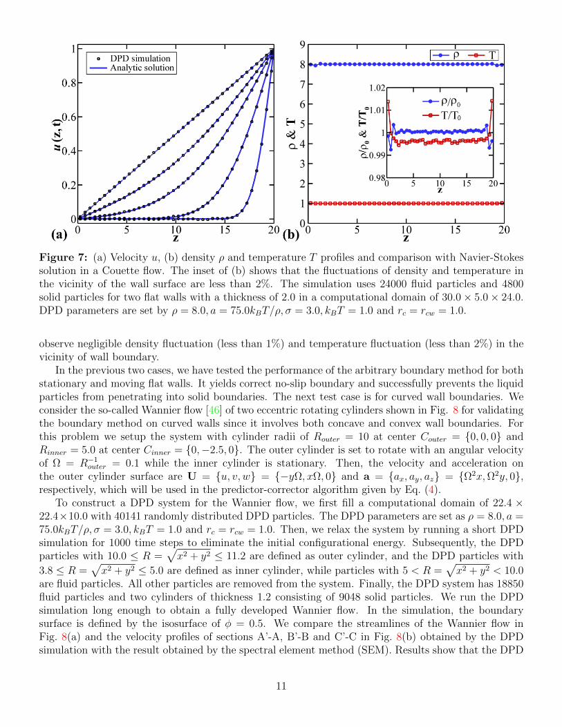
Figure 7: (a) Velocity u, (b) density ρ and temperature T profiles and comparison with Navier-Stokessolution in a Couette flow. The inset of (b) shows that the fluctuations of density and temperature inthe vicinity of the wall surface are less than 2%. The simulation uses 24000 fluid particles and 4800solid particles for two flat walls with a thickness of 2.0 in a computational domain of 30.0× 5.0× 24.0.DPD parameters are set by ρ = 8.0, a = 75.0kBT/ρ, σ = 3.0, kBT = 1.0 and rc = rcw = 1.0.

observe negligible density fluctuation (less than 1%) and temperature fluctuation (less than 2%) in thevicinity of wall boundary.

In the previous two cases, we have tested the performance of the arbitrary boundary method for bothstationary and moving flat walls. It yields correct no-slip boundary and successfully prevents the liquidparticles from penetrating into solid boundaries. The next test case is for curved wall boundaries. Weconsider the so-called Wannier flow [46] of two eccentric rotating cylinders shown in Fig. 8 for validatingthe boundary method on curved walls since it involves both concave and convex wall boundaries. Forthis problem we setup the system with cylinder radii of Router = 10 at center Couter = 0, 0, 0 andRinner = 5.0 at center Cinner = 0,−2.5, 0. The outer cylinder is set to rotate with an angular velocityof Ω = R−1

outer = 0.1 while the inner cylinder is stationary. Then, the velocity and acceleration onthe outer cylinder surface are U = u, v, w = −yΩ, xΩ, 0 and a = ax, ay, az = Ω2x,Ω2y, 0,respectively, which will be used in the predictor-corrector algorithm given by Eq. (4).

To construct a DPD system for the Wannier flow, we first fill a computational domain of 22.4 ×22.4×10.0 with 40141 randomly distributed DPD particles. The DPD parameters are set as ρ = 8.0, a =75.0kBT/ρ, σ = 3.0, kBT = 1.0 and rc = rcw = 1.0. Then, we relax the system by running a short DPDsimulation for 1000 time steps to eliminate the initial configurational energy. Subsequently, the DPDparticles with 10.0 ≤ R =

√x2 + y2 ≤ 11.2 are defined as outer cylinder, and the DPD particles with

3.8 ≤ R =√x2 + y2 ≤ 5.0 are defined as inner cylinder, while particles with 5 < R =

√x2 + y2 < 10.0

are fluid particles. All other particles are removed from the system. Finally, the DPD system has 18850fluid particles and two cylinders of thickness 1.2 consisting of 9048 solid particles. We run the DPDsimulation long enough to obtain a fully developed Wannier flow. In the simulation, the boundarysurface is defined by the isosurface of φ = 0.5. We compare the streamlines of the Wannier flow inFig. 8(a) and the velocity profiles of sections A’-A, B’-B and C’-C in Fig. 8(b) obtained by the DPDsimulation with the result obtained by the spectral element method (SEM). Results show that the DPD

11

Figure 8: (a)Streamlines of the Wannier flow and (b) velocity profiles of sections A’-A, B’-B and C’-Cobtained by the DPD simulation and the spectral element method (SEM). The DPD simulation uses18850 fluid particles and 9054 solid particles for two cylinders of thickness 1.2 in a computational domainof 22.4×22.4×10.0. The wall surface is represented by the isosurface of φ = 0.5 in the DPD simulation.

simulation is in very good agreement with the solution of SEM and we do not observe wall penetrationin the DPD simulation, which indicates that the proposed boundary method can be safely applied toproblems involving curved boundaries.

To further demonstrate the capability of the presented arbitrary boundary method in realistic ap-plication scenarios, we construct a “Brown Pacman” microfluidic device and carry out a simulation ofa surfactant solution flowing through the microfluidic channel with complex geometry [47]. The systemis set up by mapping a vector graphics image of the desired channel geometry, as shown in Fig. 9(a),onto a simulation box of size 600 × 230 × 24 reduced units. DPD particles representing the channelwall are then placed randomly within regions with brightness < 50%, while 6 341 124 solvent particlesand 300 000 surfactant particles with a volume concentration of 4.52% are randomly placed in regionswith brightness > 50%. The system comprises of a total of 13 248 000 DPD particles and the simula-tion is performed using the USER MESO GPU-accelerated DPD package [48]. Each surfactant molecule hasone hydrophilic bead (H) and one hydrophobic bead (T) connected by a harmonic bond with potentialEb(r) = K(r − r0)2, where K is the spring force constant, and r, r0 the instantaneous and equilibriumbond length. A cutoff distance rc = 1.0 is used for the pairwise interaction and rcw = 1.0 for the localdetection method. The wall surface is represented by the isosurface of φ = 0.5. The interaction ma-trix between the surfactant, solvent and wall particles is given in Table 1. A lateral pressure gradient,−∂p/∂x = c(vx− v0

x), where c = 0.25 and v0x = 4, is applied at the inlet of the channel to drive the flow.

The system is first optimized using a short run of DPD simulation. A time step size of ∆t = 0.01 isthen used to simulate the system for 1× 106 time steps.

In Fig. 9(b), we observe rich phenomena of surfactant dynamically assembling and disassemblingfollowing the flow (see also Supporting Information for the movie). Three local zoom-in views of Fig. 9(b)are shown in Fig. 9A, B and C. More specifically, zone A is located between the walls of “B” and “R”,where the flow field is almost stationary. Consequently, the surfactant molecules in a shear-free solution

12

Figure 9: (a) The vector graphical image used for generating the DPD system of a “Brown Pacman”microfluidic device. (b) Visualization of the surfactant solution flowing through the “Brown Pacman”channel (see also Supporting Information for the movie). A, B and C are three zoom-in views of (b).

self-assemble into small spherical aggregates, as shown in Fig. 9A. However, Fig. 9B shows that thesurfactant molecules form elongated wormlike micelles under strong shear flow. We observe that thesewormlike micelles flow around the small cylinders without wall penetration. Zone C is located at atransition area from a nearly stationary flow to a shear flow, where a shear-induced phase transitionfrom spherical micelles to elongated wormlike micelles is shown in Fig. 9C. Since the boundary geometryis computed on-the-fly, the proposed local detection method takes care of imposing no-slip boundaryconditions and preventing wall penetrations automatically, even for such a complex microfluidic device.This may be very valuable for many realistic applications.

Table 1: Repulsive force constants aij for microfluidic channel

H T Solvent WallH 45 75 37.5 150T 75 37.5 150 150Solvent 37.5 150 37.5 37.5Wall 150 150 37.5 37.5

4 Summary and Discussions

A local detection method tackling the challenges induced by arbitrarily shaped boundaries and complexgeometries in dissipative particle dynamics (DPD) simulations has been proposed. By computing aboundary volume fraction (BVF) for each fluid particle, the solid boundary is detected on-the-fly bythe fluid particles according to local particle configuration. At a small extra computational cost, the

13

fluid particles become autonomous to find the wall surface and to infer the wall penetration based onthe coordinates of their neighboring particles. A predictor-corrector algorithm was employed to preventthe fluid particles from penetrating into the wall boundaries, and the effective dissipative coefficients forliquid-solid interactions were used to impose no-slip boundary condition on the wall surface.

We employed randomly distributed particles to represent walls to allow easiness and generality forconstruction of DPD systems involving arbitrary-shape boundaries. Theoretically, to the limit of thecontinuum approximation, the wall surface can be accurately represented by the isosurface of BVFφ = 0.5 when the solid particles are dense enough. However, in practical implementations, the ran-dom distribution of discrete particles with finite number density will introduce surface roughness ofwall boundaries, which comes from the estimation error of BVF based on the discrete particles. Wedemonstrated that the magnitude of roughness associated with the randomness of particle distributionis monotonically controllable by tuning the cutoff radius for computing BVF and the number densityof DPD particles. Since any natural solid wall contains more or less chemical/physical heterogeneitieson the surface, especially at the mesoscopic scale, such heterogeneity can be modeled qualitatively bythe roughness on walls in the DPD systems. In this respect, the proposed boundary method provides aconvenient way to generate various sizes of the roughness for representation of different degrees of theheterogeneity and to introduce curvature-dependent slip for hydrodynamics as discussed in the A.

The transition Poiseuille and Couette flows as well as the Wannier flow were used as benchmark testsfor verifying the proposed arbitrary boundary method. The results showed that the proposed boundarymethod imposes the correct no-slip boundary condition for both stationary and moving walls in theDPD simulation, and yields negligible density fluctuation (less than 1%) and temperature fluctuation(less than 2%) in the vicinity of wall surface. To further demonstrate the capability of the presentedarbitrary boundary method in realistic application scenarios, a “Brown Pacman” microfluidic devicewith complex geometry was constructed directly from a vector graphics image and a DPD simulationof surfactant solution flowing through this complex microfluidic device was carried out. The validityof this boundary method is confirmed by examining the rich dynamics of surfactant micelles flowingaround the small cylinders without wall penetration.

Since this local detection method only uses local information of neighboring particles for computingthe value of BVF and satisfies designed boundary conditions on-the-fly, it provides a practical andefficient way to deal with complex geometries and impose the no-slip boundary condition on wall surfacein DPD simulations. With the local detection method, it is no longer necessary to mathematically definethe boundary geometry for DPD simulations, which enables us to construct DPD systems directlyfrom experimental CT images or computer-aided designs/drawings. Moreover, this method is not onlyvaluable for stationary arbitrary-shape boundaries, but also for the moving boundaries and deformableboundaries.

Although we presented here that the surface roughness is controllable by varying the number ofneighboring particles, this boundary method cannot accurately capture large curvatures of wall boundarywhere the radius of curvature is too small to be identified from the surface roughness. To this end, higherresolution of DPD system is required to represent the large curvature properly so that the size of randomsurface roughness is much smaller than the radius of curvature.

Acknowledgements

This work was primarily supported by the DOE Center on Mathematics for Mesoscopic Modeling ofMaterials (CM4). This work was also sponsored by the U.S. Army Research Laboratory and wasaccomplished under Cooperative Agreement Number W911NF-12-2-0023 to University of Utah. An

14

award of computer time was provided by the Innovative and Novel Computational Impact on Theoryand Experiment (INCITE) program with the resources of the Argonne Leadership Computing Facility(ALCF) and the resources of the Oak Ridge Leadership Computing Facility (OLCF). Z. Li would liketo thank Dr. Yue Yu for her support on running the spectral element simulation of the Wannier flow.

A Error Analysis for Curved Surfaces

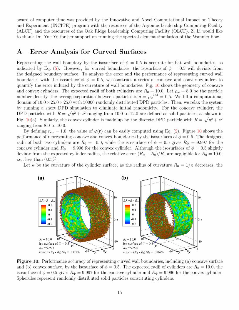
Representing the wall boundary by the isosurface of φ = 0.5 is accurate for flat wall boundaries, asindicated by Eq. (5). However, for curved boundaries, the isosurface of φ = 0.5 will deviate fromthe designed boundary surface. To analyze the error and the performance of representing curved wallboundaries with the isosurface of φ = 0.5, we construct a series of concave and convex cylinders toquantify the error induced by the curvature of wall boundaries. Fig. 10 shows the geometry of concaveand convex cylinders. The expected radii of both cylinders are R0 = 10.0. Let ρw = 8.0 be the particlenumber density, the average separation between particles is δ = ρ

−1/3w = 0.5. We fill a computational

domain of 10.0×25.0×25.0 with 50000 randomly distributed DPD particles. Then, we relax the systemby running a short DPD simulation to eliminate initial randomicity. For the concave cylinder, theDPD particles with R =

√y2 + z2 ranging from 10.0 to 12.0 are defined as solid particles, as shown in

Fig. 10(a). Similarly, the convex cylinder is made up by the discrete DPD particle with R =√y2 + z2

ranging from 8.0 to 10.0.By defining rcw = 1.0, the value of ϕ(r) can be easily computed using Eq. (2). Figure 10 shows the

performance of representing concave and convex boundaries by the isosurfaces of φ = 0.5. The designedradii of both two cylinders are R0 = 10.0, while the iso-surface of φ = 0.5 gives RΦ = 9.997 for theconcave cylinder and RΦ = 9.996 for the convex cylinder. Although the isosurfaces of φ = 0.5 slightlydeviate from the expected cylinder radius, the relative error (RΦ −R0)/R0 are negligible for R0 = 10.0,i.e., less than 0.05%.

Let κ be the curvature of the cylinder surface, as the radius of curvature R0 = 1/κ decreases, the

Figure 10: Performance accuracy of representing curved wall boundaries, including (a) concave surfaceand (b) convex surface, by the isosurface of φ = 0.5. The expected radii of cylinders are R0 = 10.0, theisosurface of φ = 0.5 gives RΦ = 9.997 for the concave cylinder and RΦ = 9.996 for the convex cylinder.Spherules represent randomly distributed solid particles constituting cylinders.

15

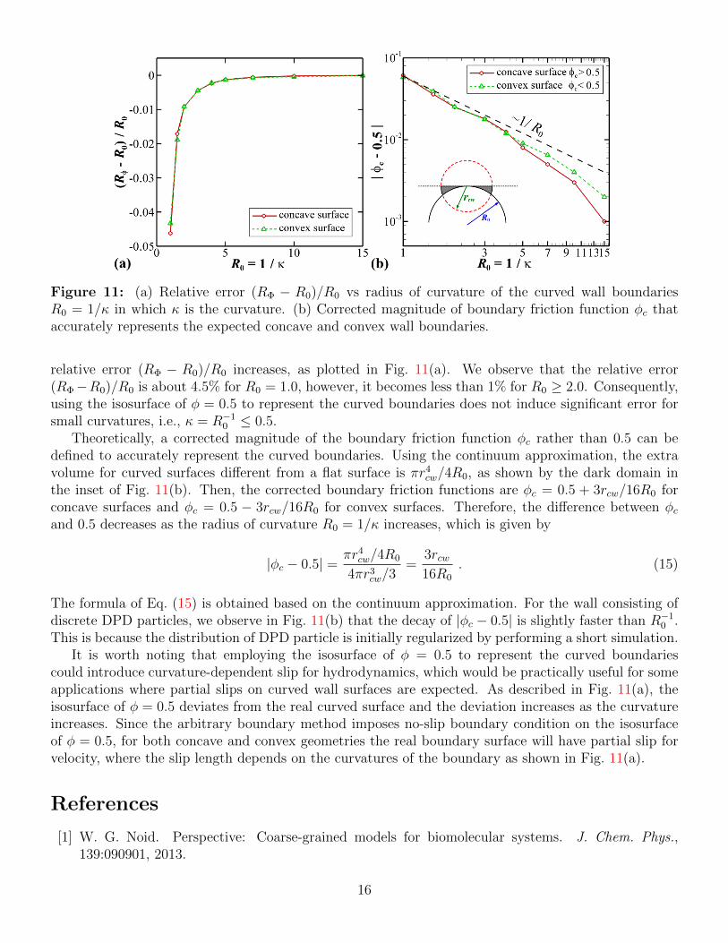
Figure 11: (a) Relative error (RΦ − R0)/R0 vs radius of curvature of the curved wall boundariesR0 = 1/κ in which κ is the curvature. (b) Corrected magnitude of boundary friction function φc thataccurately represents the expected concave and convex wall boundaries.

relative error (RΦ − R0)/R0 increases, as plotted in Fig. 11(a). We observe that the relative error(RΦ−R0)/R0 is about 4.5% for R0 = 1.0, however, it becomes less than 1% for R0 ≥ 2.0. Consequently,using the isosurface of φ = 0.5 to represent the curved boundaries does not induce significant error forsmall curvatures, i.e., κ = R−1

0 ≤ 0.5.Theoretically, a corrected magnitude of the boundary friction function φc rather than 0.5 can be

defined to accurately represent the curved boundaries. Using the continuum approximation, the extravolume for curved surfaces different from a flat surface is πr4

cw/4R0, as shown by the dark domain inthe inset of Fig. 11(b). Then, the corrected boundary friction functions are φc = 0.5 + 3rcw/16R0 forconcave surfaces and φc = 0.5 − 3rcw/16R0 for convex surfaces. Therefore, the difference between φcand 0.5 decreases as the radius of curvature R0 = 1/κ increases, which is given by

|φc − 0.5| = πr4cw/4R0

4πr3cw/3

=3rcw16R0

. (15)

The formula of Eq. (15) is obtained based on the continuum approximation. For the wall consisting ofdiscrete DPD particles, we observe in Fig. 11(b) that the decay of |φc − 0.5| is slightly faster than R−1

0 .This is because the distribution of DPD particle is initially regularized by performing a short simulation.

It is worth noting that employing the isosurface of φ = 0.5 to represent the curved boundariescould introduce curvature-dependent slip for hydrodynamics, which would be practically useful for someapplications where partial slips on curved wall surfaces are expected. As described in Fig. 11(a), theisosurface of φ = 0.5 deviates from the real curved surface and the deviation increases as the curvatureincreases. Since the arbitrary boundary method imposes no-slip boundary condition on the isosurfaceof φ = 0.5, for both concave and convex geometries the real boundary surface will have partial slip forvelocity, where the slip length depends on the curvatures of the boundary as shown in Fig. 11(a).

References

[1] W. G. Noid. Perspective: Coarse-grained models for biomolecular systems. J. Chem. Phys.,139:090901, 2013.

16

[2] E. Brini, E. A. Algaer, P. Ganguly, C. L. Li, F. Rodriguez-Ropero, and N. F. A. van der Vegt.Systematic coarse-graining methods for soft matter simulations - a review. Soft Matter, 9(7):2108–2119, 2013.

[3] S. Yip and M. P. Short. Multiscale materials modelling at the mesoscale. Nat. Mater., 12(9):774–777, 2013.

[4] Z. G. Mills, W. B. Mao, and A. Alexeev. Mesoscale modeling: solving complex flows in biology andbiotechnology. Trends Biotechnol., 31(7):426–434, 2013.

[5] M. G. Saunders and G. A. Voth. Coarse-graining methods for computational biology. Annu. Rev.Biophys., 42:73–93, 2013.

[6] Z. Li, Y.-H. Tang, X. J. Li, and G. E. Karniadakis. Mesoscale modeling of phase transition dynamicsof thermoresponsive polymers. Chem. Commun., 51(55):11038–11040, 2015.

[7] M. Lisal, Z. Limpouchova, and K. Prochazka. The self-assembly of copolymers with one hydrophobicand one polyelectrolyte block in aqueous media: a dissipative particle dynamics study. Phys. Chem.Chem. Phys., 18(24):16127–16136, 2016.

[8] D. Y. Pan, J. X. Hu, and X. M. Shao. Lees-Edwards boundary condition for simulation of polymersuspension with dissipative particle dynamics method. Mol. Simul., 42(4):328–336, 2016.

[9] X. Bian, S. Litvinov, R. Qian, M. Ellero, and N. A. Adams. Multiscale modeling of particle insuspension with smoothed dissipative particle dynamics. Phys. Fluids, 24(1), 2012.

[10] R. G. Winkler, D. A. Fedosov, and G. Gompper. Dynamical and rheological properties of softcolloid suspensions. Curr. Opin. Colloid Interface Sci., 19(6):594–610, 2014.

[11] D. S. Bolintineanu, G. S. Grest, J. B. Lechman, F. Pierce, S. J. Plimpton, and P. R. Schunk.Particle dynamics modeling methods for colloid suspensions. Comp. Part. Mech., 1(3):321–356,2014.

[12] Z. Li, G. H. Hu, Z. L. Wang, Y. B. Ma, and Z. W. Zhou. Three dimensional flow structures ina moving droplet on substrate: A dissipative particle dynamics study. Phys. Fluids, 25(7):072103,2013.

[13] Y. X. Wang and S. Chen. Numerical study on droplet sliding across micropillars. Langmuir,31(16):4673–4677, 2015.

[14] K. Yang and Z. L. Guo. Lattice Boltzmann study of wettability alteration in the displacement ofnanoparticle-filled binary fluids. Computers & Fluids, 124:157–169, 2016.

[15] T. Ye, N. Phan-Thien, B. C. Khoo, and C. T. Lim. Dissipative particle dynamics simulations ofdeformation and aggregation of healthy and diseased red blood cells in a tube flow. Phys. Fluids,26(11):111902, 2014.

[16] I. V. Pivkin, Z. L. Peng, G. E. Karniadakis, P. A. Buffet, M. Dao, and S. Suresh. Biomechanicsof red blood cells in human spleen and consequences for physiology and disease. Proc. Natl. Acad.Sci. U. S. A., 113(28):7804–7809, 2016.

17

[17] H. Y. Chang, X. J. Li, H. Li, and G. E. Karniadakis. MD/DPD multiscale framework for pre-dicting morphology and stresses of red blood cells in health and disease. PLoS Comput. Biol.,12(10):e1005173, 2016.

[18] H. Lei, D. A. Fedosov, B. Caswell, and G. E. Karniadakis. Blood flow in small tubes: quantifyingthe transition to the non-continuum regime. J. Fluid Mech., 722:214–239, 2013.

[19] E. Henry, S. H. Holm, Z. M. Zhang, J. P. Beech, J. O. Tegenfeldt, D. A. Fedosov, and G. Gompper.Sorting cells by their dynamical properties. Scientific Reports, 6:34375, 2016.

[20] X. J. Li, E. Du, H. Lei, Y.-H. Tang, M. Dao, S. Suresh, and G. E. Karniadakis. Patient-specificblood rheology in sickle-cell anaemia. Interface Focus, 6(1):20150065, 2016.

[21] X. J. Li, B. Caswell, and G. E. Karniadakis. Effect of chain chirality on the self-assembly of sicklehemoglobin. Biophys. J., 103(6):1130–1140, 2012.

[22] J. Zavadlav, M. N. Melo, S. J. Marrink, and M. Praprotnik. Adaptive resolution simulation of anatomistic protein in MARTINI water. J. Chem. Phys., 140(5):054114, 2014.

[23] Y.-H. Tang, Z. Li, X. J. Li, M. G. Deng, and G. E. Karniadakis. Non-equilibrium dynamics ofvesicles and micelles by self-assembly of block copolymers with double thermoresponsivity. Macro-molecules, 49(7):2895–2903, 2016.

[24] P.J Hoogerbrugge and J.M.V.A Koelman. Simulating microscopic hydrodynamic phenomena withdissipative particle dynamics. Europhys. Lett., 19(3):155–160, 1992.

[25] D. A. Fedosov, H. Noguchi, and G. Gompper. Multiscale modeling of blood flow: from single cellsto blood rheology. Biomech. Model. Mechanobiol., 13(2):239–258, 2014.

[26] M. B. Liu, G. R. Liu, L. W. Zhou, and J. Z. Chang. Dissipative particle dynamics (DPD): Anoverview and recent developments. Arch. Comput. Method E., 22(4):529–556, 2015.

[27] Z. Li, X. Bian, B. Caswell, and G. E. Karniadakis. Construction of dissipative particle dynamicsmodels for complex fluids via the Mori-Zwanzig formulation. Soft Matter, 10(43):8659–8672, 2014.

[28] Z. Li, X. Bian, X. T. Li, and G. E. Karniadakis. Incorporation of memory effects in coarse-grainedmodeling via the Mori-Zwanzig formalism. J. Chem. Phys., 143(24):243128, 2015.

[29] R. D. Groot and P. B. Warren. Dissipative particle dynamics: Bridging the gap between atomisticand mesoscopic simulation. J. Chem. Phys., 107(11):4423–4435, 1997.

[30] P. Espanol and P. Warren. Statistical mechanics of dissipative particle dynamics. Europhys. Lett.,30(4):191–196, 1995.

[31] R. Kubo. The fluctuation-dissipation theorem. Rep. Prog. Phys., 29(1):255–284, 1966.

[32] M. P. Allen and D. J. Tildesley. Computer simulation of liquids. Clarendon Press, New York, 1989.

[33] S. Adami, X. Y. Hu, and N. A. Adams. A generalized wall boundary condition for smoothed particlehydrodynamics. J. Comput. Phys., 231(21):7057–7075, 2012.

[34] I. V. Pivkin and G. E. Karniadakis. A new method to impose no-slip boundary conditions indissipative particle dynamics. J. Comput. Phys., 207:114–128, 2005.

18

[35] P. J. Colmenares and R. Rousse. Effective boundary forces for several geometries in dissipativeparticle dynamics. Physica A, 367:93–105, 2006.

[36] A. M. Altenhoff, J. H. Walther, and P. Koumoutsakos. A stochastic boundary forcing for dissipativeparticle dynamics. J. Comput. Phys., 225:1125–1136, 2007.

[37] M. Revenga, I. Zuniga, and P. Espanol. Boundary conditions in dissipative particle dynamics.Comput. Phys. Commun., 121(122):309–311, 1999.

[38] G.R. Liu and M.B. Liu. Smoothed Particle Hydrodynamics: A Meshfree Particle Method. WorldScientific, 2003.

[39] J. J. Monaghan. Smoothed particle hydrodynamics. Rep. Prog. Phys., 68(8):1703–1759, 2005.

[40] L. B. Lucy. A numerical approach to the testing of the fission hypothesis. Astron. J., 82(12):1013–1024, 1977.

[41] D. P. Kroese, T. Taimre, and Z. I. Botev. Handbook of Monte Carlo Methods. John Wiley & Sons,Inc., 2011.

[42] Z. Li, Y.-H. Tang, H. Lei, B. Caswell, and G. E. Karniadakis. Energy-conserving dissipative particledynamics with temperature-dependent properties. J. Comput. Phys., 265:113–127, 2014.

[43] L. D. G. Sigalotti, J. Klapp, E. Sira, Y. Melean, and A. Hasmy. SPH simulations of time-dependentpoiseuille flow at low reynolds numbers. J. Comput. Phys., 191(2):622–638, 2003.

[44] J. A. Backer, C. P. Lowe, H. C. J. Hoefsloot, and P. D. Iedema. Poiseuille flow to measure theviscosity of particle model fluids. J. Chem. Phys., 122(15), 2005.

[45] Z. Li, A. Yazdani, A. Tartakovsky, and G. E. Karniadakis. Transport dissipative particle dynamicsmodel for mesoscopic advection-diffusion-reaction problems. J. Chem. Phys., 143(1):014101, 2015.

[46] G. H. Wannier. A contribution to the hydrodynamics of lubrication. Q. Appl. Math., 8(1):1–32,1950.

[47] M. Li, M. Humayun, J. A Kozinski, and D. K. Hwang. Functional polymer sheet patterning usingmicrofluidics. Langmuir, 30(28):8637–8644, 2014.

[48] Y.-H. Tang and G. E. Karniadakis. Accelerating dissipative particle dynamics simulations on GPUs:Algorithms, numerics and applications. Comput. Phys. Commun., 185(11):2809–2822, 2014.

19