Dissipative particle dynamics Dissipative particle dynamics and fluid particle methodand fluid particle method

by Witold by Witold DzwinelDzwinel

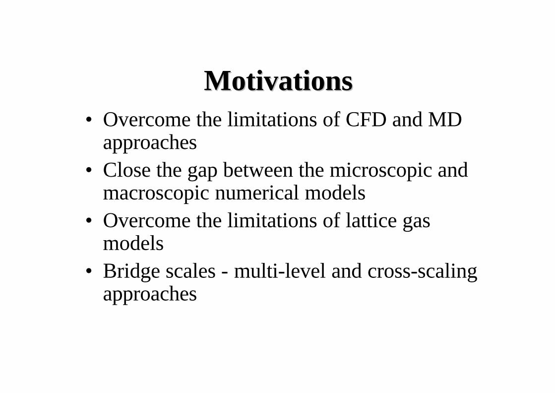
MotivationsMotivations• Overcome the limitations of CFD and MD

approaches• Close the gap between the microscopic and

macroscopic numerical models• Overcome the limitations of lattice gas

models• Bridge scales - multi-level and cross-scaling

approaches

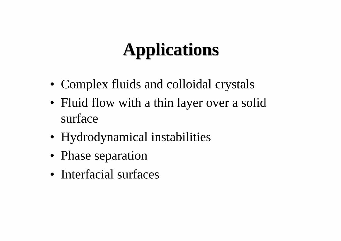
ApplicationsApplications

• Complex fluids and colloidal crystals• Fluid flow with a thin layer over a solid

surface• Hydrodynamical instabilities• Phase separation• Interfacial surfaces

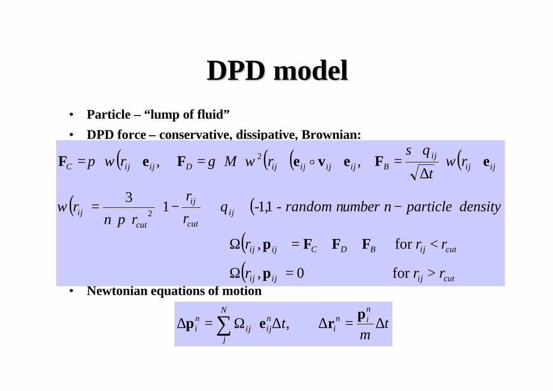
DPD modelDPD model• Particle – “lump of fluid”• DPD force – conservative, dissipative, Brownian:

• Newtonian equations of motion

( ) ( ) ( ) ( )

( ) ( )

( )( ) cutijijij

cutijBDCijij

ijcut

ij

cutij

ijijij

BijijijijDijijC

rrr

rrr

densityparticlenumber- random n,-r

r

rnr

rt

rMr

>=Ω

<++=Ω

−∈

−

⋅=

⋅⋅∆

⋅=⋅⋅⋅⋅=⋅⋅=

for 0,

for ,

11 1 3

, ,

2

2

p

FFFp

eFeveFeF

θπ

ω

ωθσ

ωγωπ o

tm

tnin

inij

N

jij

ni ∆=∆∆⋅Ω=∆ ∑ p

rep ,

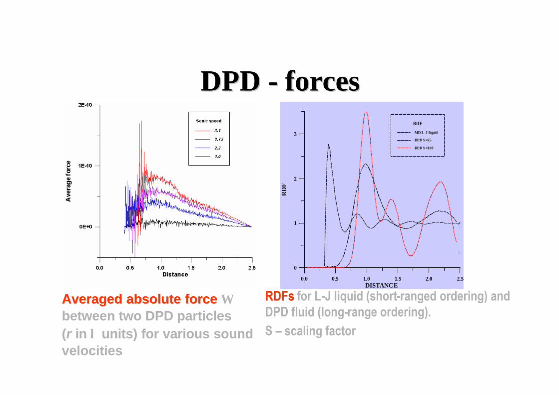
DPD DPD -- forcesforces

Averaged absolute forceAveraged absolute force Ωbetween two DPD particles (r in λ units) for various soundvelocities

0.0 0.5 1.0 1.5 2.0 2.5DISTANCE

0

1

2

3

RD

F

RDF

MD L -J liquid

DPD S=25

DPD S=100

RDFsRDFs for L-J liquid (short-ranged ordering) and DPD fluid (long-range ordering).S – scaling factor

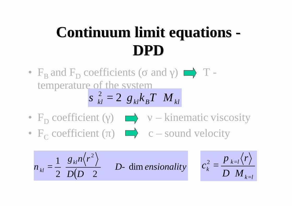
Continuum limit equations Continuum limit equations --DPDDPD

• FB and FD coefficients (σ and γ) T -temperature of the system

• FD coefficient (γ) ν – kinematic viscosity• FC coefficient (π) c – sound velocity

klBklkl MTk ⋅⋅= γσ 22

lk

lkk MD

rc

=

=

⋅=

π2

( ) yensionalitD- DD

rnklkl dim

221

2

+⋅=

γν

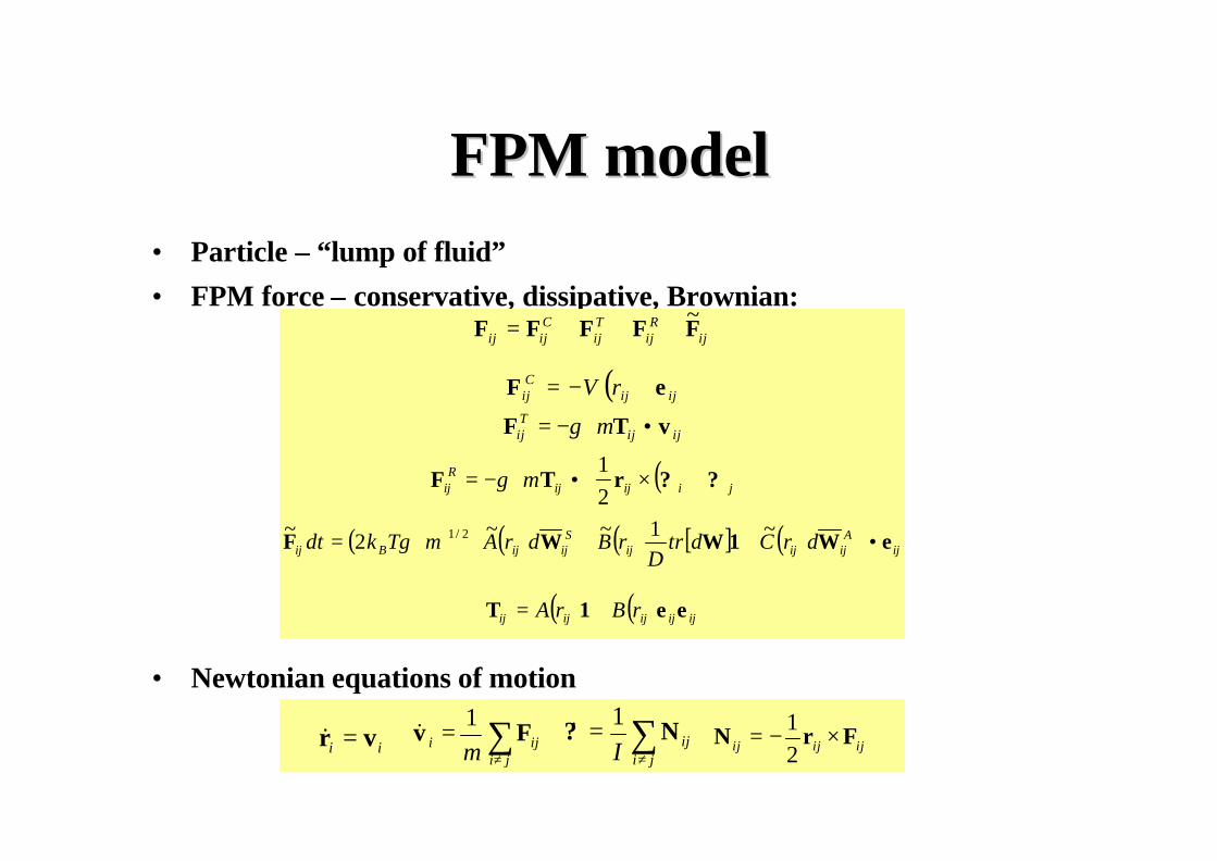
FPM modelFPM model• Particle – “lump of fluid”• FPM force – conservative, dissipative, Brownian:

• Newtonian equations of motion

ijR

ijTij

Cijij FFFFF ~+++=

( ) ijijCij rV eF ⋅−=

ijijTij m vTF •⋅−= γ

( )

+ו⋅−= jiijij

Rij m ??rTF

21

γ

( ) ( ) ( ) [ ] ( ) ijA

ijijijS

ijijBij drCdtrD

rBdrAmTkdt eW1WWF •

++⋅= ~1~~2~ 2/1γ

( ) ( ) ijijijijij rBrA ee1T +=

ii vr =&

∑≠

=ji

iji mFv

1& ∑

≠

=ji

ijIN? 1&

ijijij FrN ×−=

21

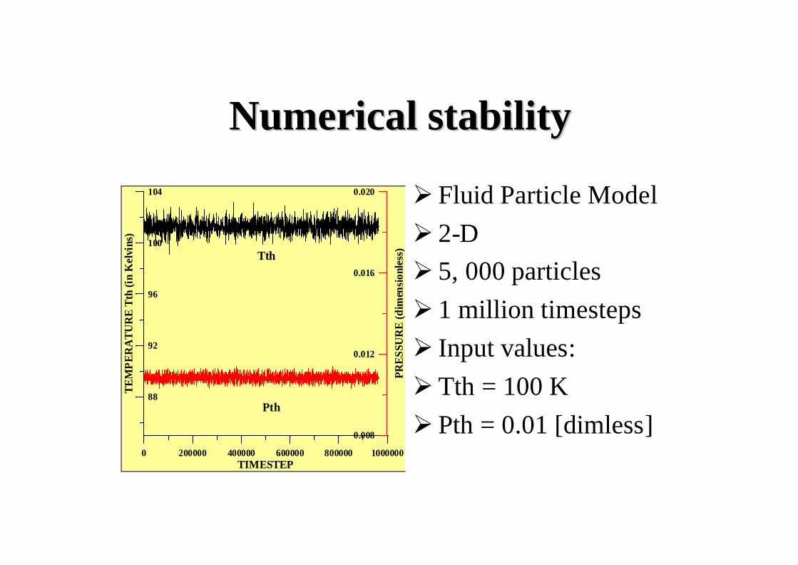
NumericalNumerical stabilitystability

0 200000 400000 600000 800000 1000000TIMESTEP

88

92

96

100

104

TE

MP

ER

AT

UR

E T

th (i

n K

elvi

ns)

0.008

0.012

0.016

0.020

PRE

SSU

RE

(dim

ensi

onle

ss)

Tth

Pth

Ø Fluid Particle ModelØ 2-DØ 5, 000 particlesØ 1 million timestepsØ Input values:ØTth = 100 KØ Pth = 0.01 [dimless]

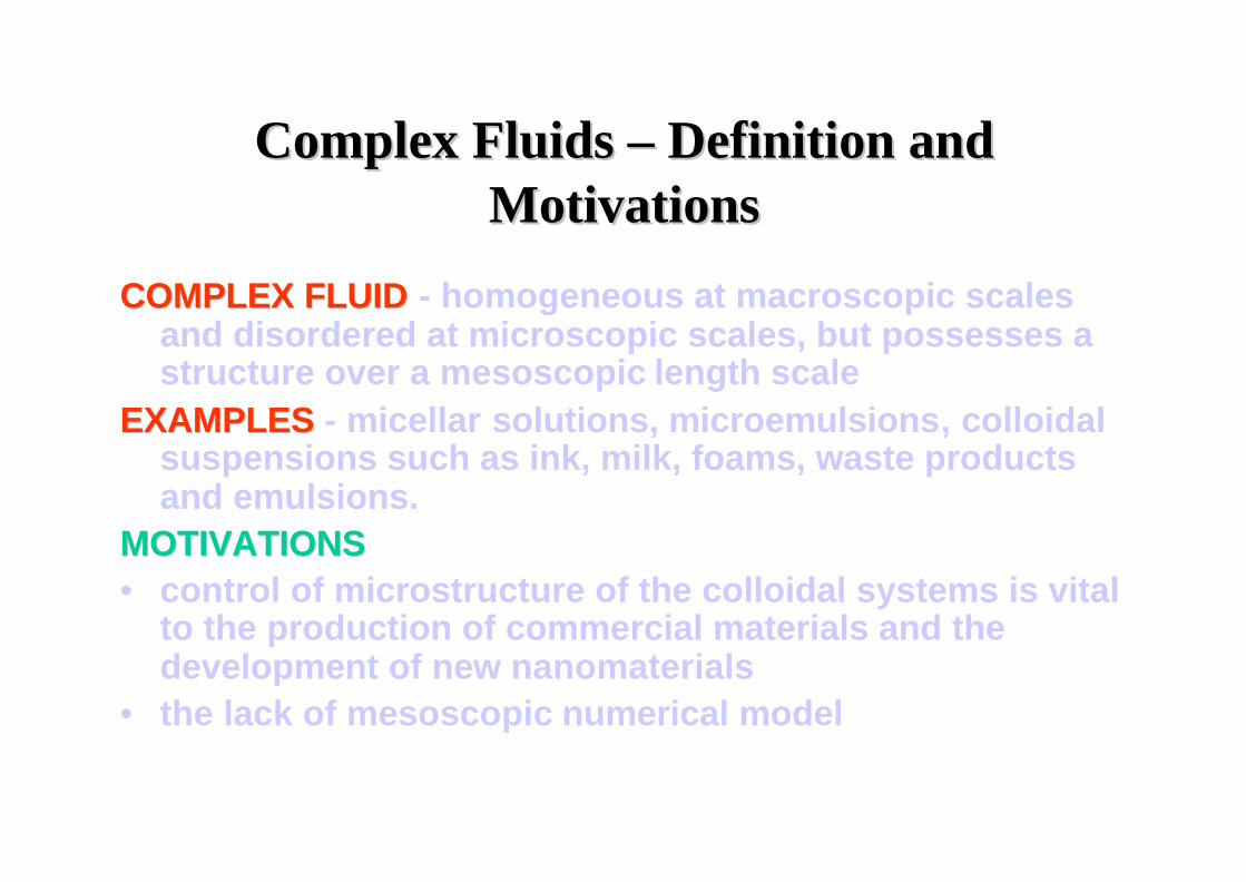
Complex Fluids Complex Fluids –– Definition and Definition and MotivationsMotivations

COMPLEX FLUIDCOMPLEX FLUID - homogeneous at macroscopic scales and disordered at microscopic scales, but possesses a structure over a mesoscopic length scale

EXAMPLESEXAMPLES - micellar solutions, microemulsions, colloidal suspensions such as ink, milk, foams, waste products and emulsions.

MOTIVATIONSMOTIVATIONS• control of microstructure of the colloidal systems is vital

to the production of commercial materials and the development of new nanomaterials

• the lack of mesoscopic numerical model

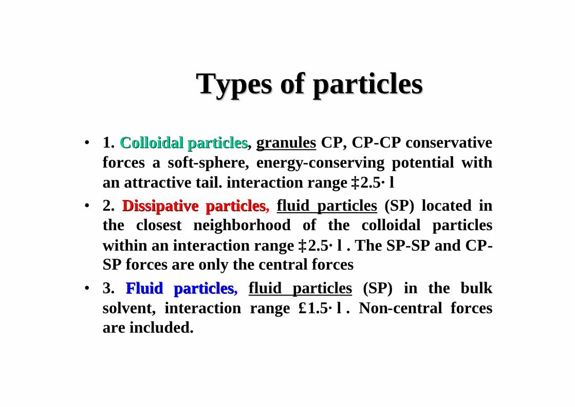
TypesTypes ofof particlesparticles

• 1. Colloidal particlesColloidal particles, granules CP, CP-CP conservative forces a soft-sphere, energy-conserving potential with an attractive tail. interaction range ≥2.5×λ

• 2. Dissipative particlesDissipative particles, fluid particles (SP) located in the closest neighborhood of the colloidal particles within an interaction range ≥2.5×λ. The SP-SP and CP-SP forces are only the central forces

• 3. Fluid particlesFluid particles, fluid particles (SP) in the bulk solvent, interaction range ≤1.5×λ. Non-central forces are included.

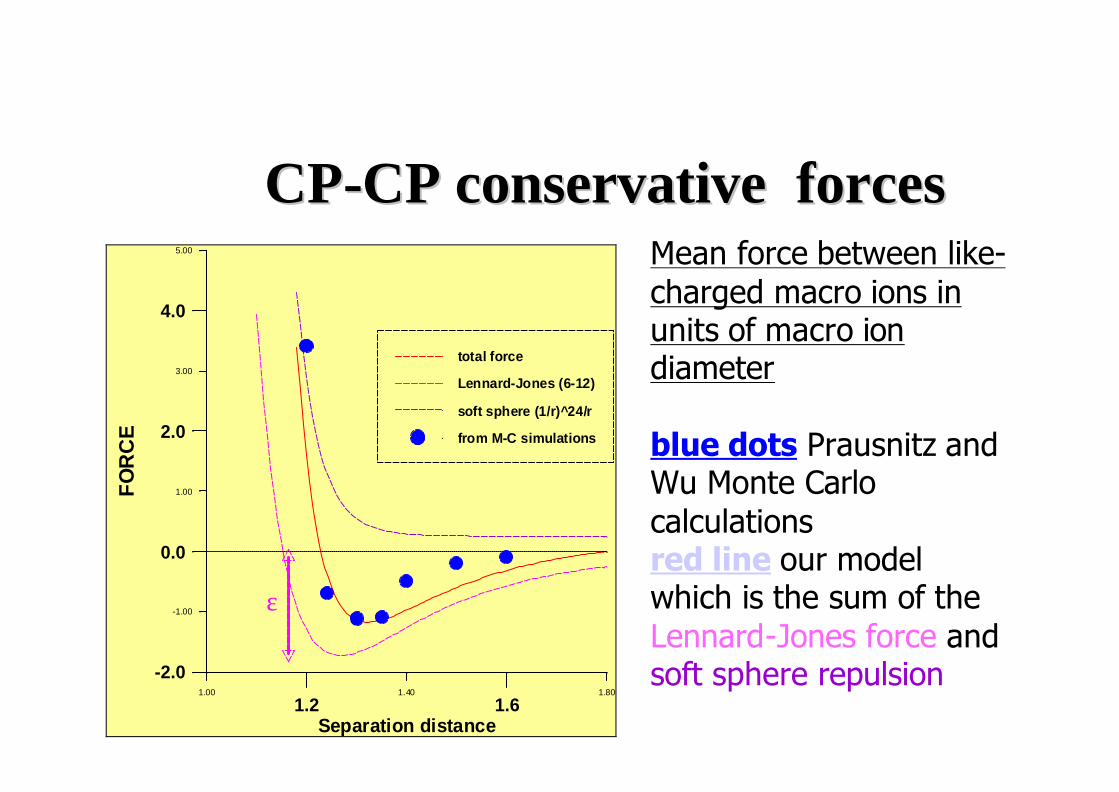
CPCP--CPCP cconservative onservative forcesforces

1.00 1.40 1.80

1.2 1.6Separation distance

-1.00

1.00

3.00

5.00

-2.0

0.0

2.0

4.0

FO

RC

E

total force

Lennard-Jones (6-12)

soft sphere (1/r)^24/r

from M-C simulations

∼ε

Mean force between like-charged macro ions inunits of macro iondiameter

blue dots Prausnitz andWu Monte Carlocalculationsred line our model which is the sum of theLennard-Jones force andsoft sphere repulsion

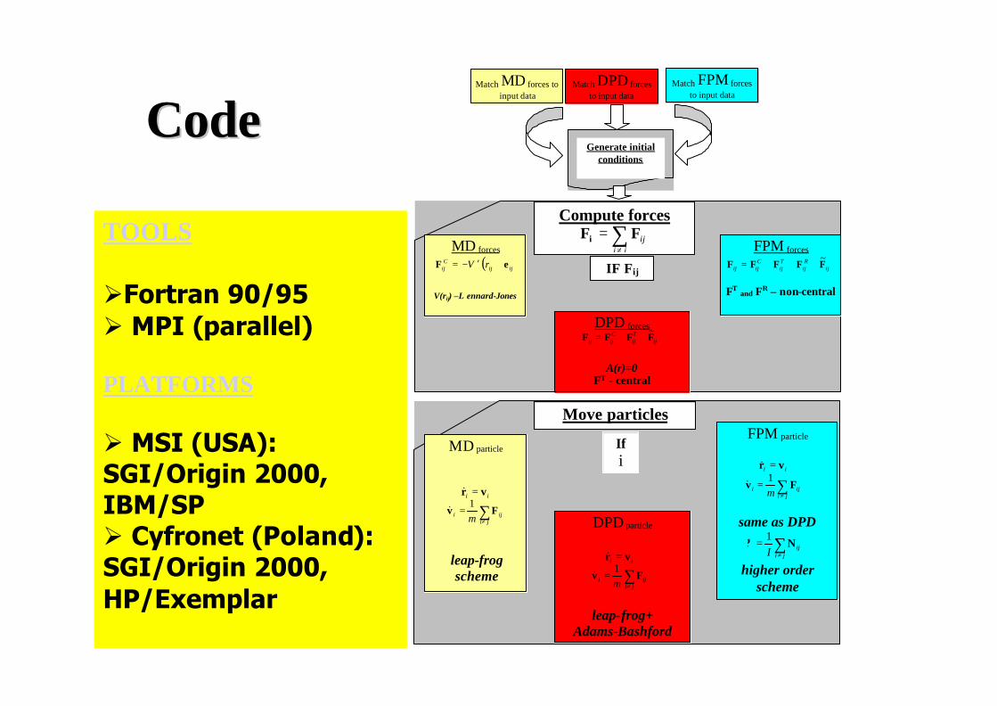
Match MD forces to

input data Match DPD forces

to input data Match FPM forces

to input data

Generate initial conditions

Compute forces ∑

≠

=ji

ijFFi

MD forces ( ) ijij

Cij rV eF ⋅′−=

V(rij) –L ennard-Jones

DPD forces ij

Tij

Cijij FFFF

~++=

A(r)=0

FT - central

FPM forces

ijR

ijTij

Cijij FFFFF

~+++=

FT and FR – non-central

Move particles If i

MD particle

ii vr =& ∑

≠

=ji

iji mFv

1&

leap-frog scheme

DPD particle

ii vr =& ∑

≠

=ji

iji mFv

1&

leap-frog+ Adams-Bashford

scheme

FPM particle

ii vr =&

∑≠

=ji

iji mFv

1&

same as DPD

∑≠

=ji

ijIN?

1&

higher order scheme

IF Fij

CodeCode

TOOLS

ØFortran 90/95Ø MPI (parallel)

PLATFORMS

Ø MSI (USA): SGI/Origin 2000, IBM/SPØ Cyfronet (Poland): SGI/Origin 2000, HP/Exemplar

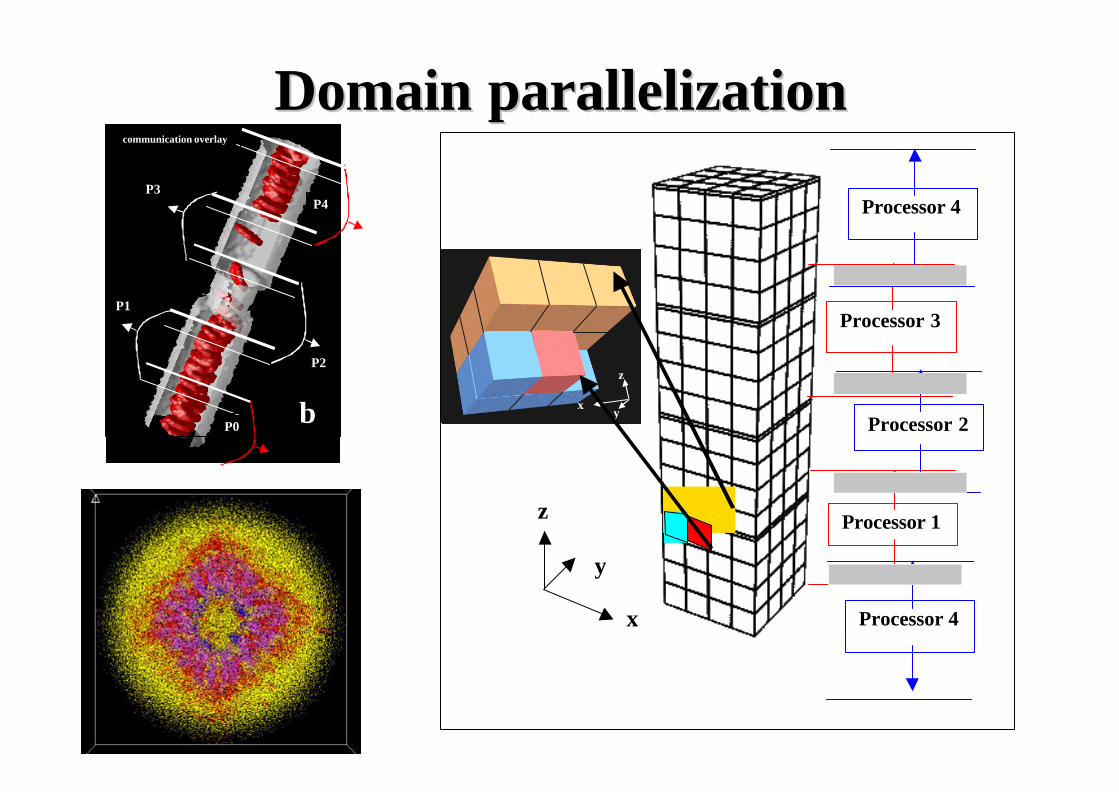
DomainDomain parallelizationparallelization

Processor 1

Processor 2

Processor 3

Processor 4

Processor 4 x

y

z

z

x y

P1

P3

P2

P4

P0

communication overlay

b

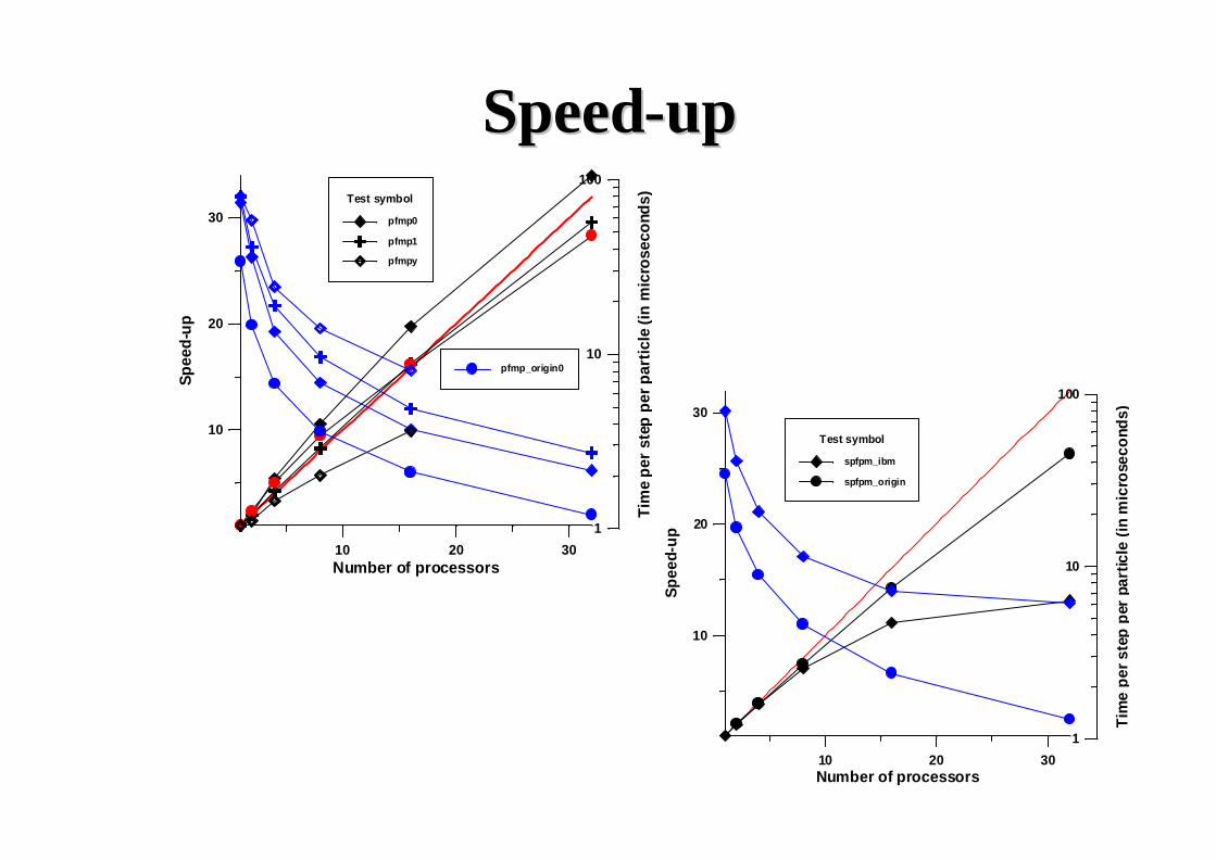
SpeedSpeed--upup

10 20 30Number of processors

10

20

30

Sp

eed

-up

1

10

100

Tim

e p

er s

tep

per

par

ticl

e (i

n m

icro

seco

nds)Test symbol

pfmp0

pfmp1

pfmpy

pfmp_origin0

10 20 30Number of processors

10

20

30

Sp

eed-

up

1

10

100

Tim

e p

er s

tep

per

par

ticle

(in

mic

rose

cond

s)

Test symbol

spfpm_ibm

spfpm_origin

Colloidal CrystalsColloidal Crystals

Ø Micelle structures obtained in DPD-MD simulations

• Comparison of simulations (a) with real colloidal arrays (b)

Ø Metastable colloidal arrays

Ø In (b) the tetrametric protein streptavidin bounded to a pariallybiotinylated lipid monolayer

b

a b

a

Fluid Flow With a Thin Layer Over a Solid Fluid Flow With a Thin Layer Over a Solid SurfaceSurface MotivationsMotivations

•• TECHNOLOGICAL IMPORTANCETECHNOLOGICAL IMPORTANCEØ spin coating of microchipsØ fast drying paint productionØ design of photographic films

•• OVERCOME PROBLEMS WITH CONTINUUM OVERCOME PROBLEMS WITH CONTINUUM EQUATIONSEQUATIONS (Evolutionary Equation-EE)

Ø moving boundary conditions: creation of holes, spreading of fronts, development of fingers

Ø EE solution exhibits steepening of the wavefronts, leading to wave-breaking in a finite time

Ø Overcome limits of validity of the approximate theories

Fluid Flow With a Thin Layer Over a Solid Fluid Flow With a Thin Layer Over a Solid SurfaceSurface MODELMODEL

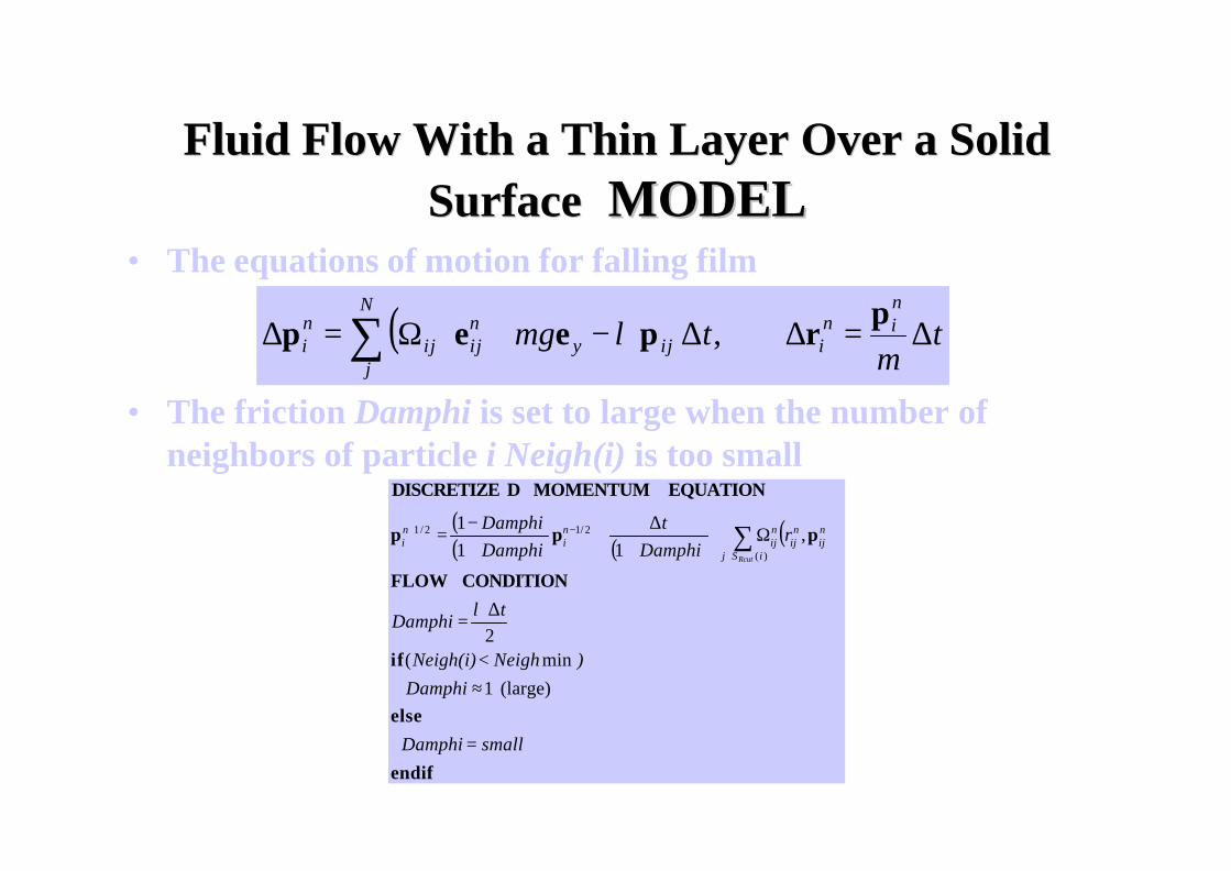
• The equations of motion for falling film

• The friction Damphi is set to large when the number of neighbors of particle i Neigh(i) is too small

( )( ) ( )

( )

endif

else

if

CONDITION FLOW

ppp

EQUATION MOMENTUM DDISCRETIZE

smallDamphi

Damphi)NeighNeigh(i)

tDamphi

rDamphi

tDamphiDamphi

iSj

nij

nij

nij

ni

ni

Rcut

=

≈<

∆=

Ω

+∆

++−

= ∑∈

−+

(large) 1 min(

2

,11

1

)(

2/12/1

λ

( ) tm

tmgnin

i

N

jijy

nijij

ni ∆=∆∆−+⋅Ω=∆ ∑ p

rpeep , λ

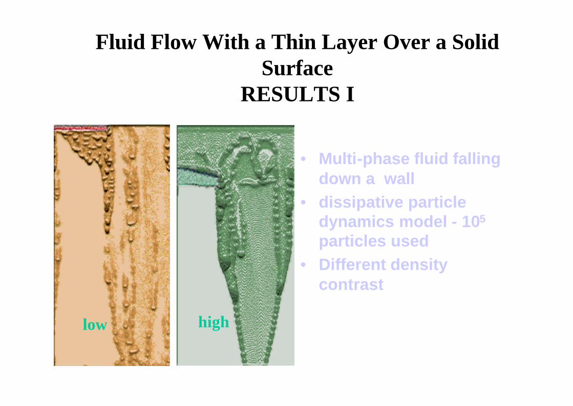
Fluid Flow With a Thin Layer Over a Solid Surface

RESULTS I

• Multi-phase fluid falling down a wall

• dissipative particle dynamics model - 105

particles used• Different density

contrast

low high

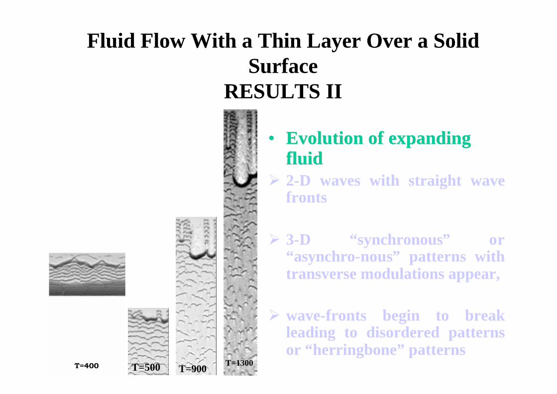
Fluid Flow With a Thin Layer Over a Solid Surface

RESULTS II

•• Evolution of expanding Evolution of expanding fluidfluid

Ø 2-D waves with straight wave fronts

Ø 3-D “synchronous” or “asynchro-nous” patterns with transverse modulations appear,

Ø wave-fronts begin to break leading to disordered patterns or “herringbone” patterns

T=500 T=900T=1300T=400

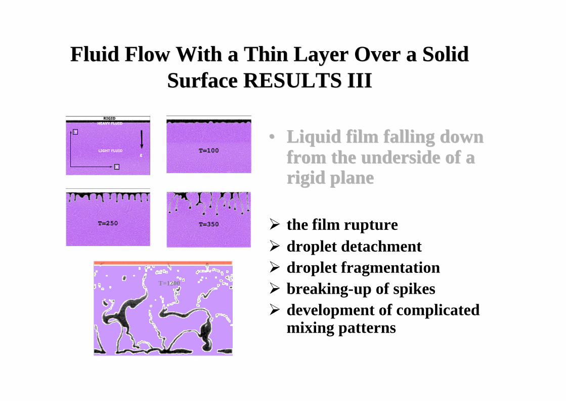
Fluid Flow With a Thin Layer Over a Solid Fluid Flow With a Thin Layer Over a Solid SurfaceSurface RESULTS IIIRESULTS III

•• Liquid film falling down Liquid film falling down from the underside of a from the underside of a rigid planerigid plane

Ø the film ruptureØ droplet detachment Ø droplet fragmentation Ø breaking-up of spikesØ development of complicated

mixing patterns

RIGID

LIGHT FLUID

HEAVY FLUID

g

Y

X

T=100

T=100 T=100 T=100T=100

T=250 T=350

T=1200

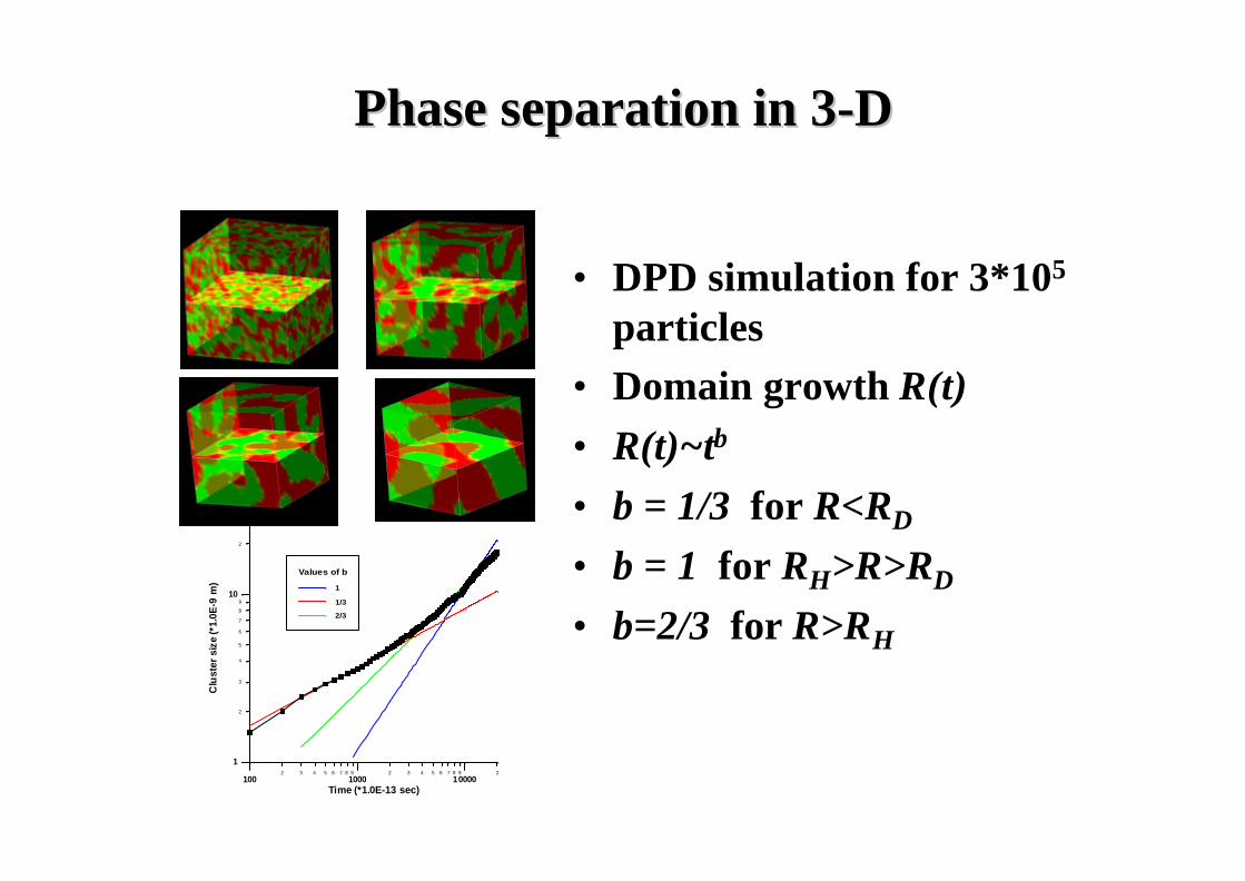
Phase separation in 3Phase separation in 3--DD

• DPD simulation for 3*105

particles • Domain growth R(t)• R(t)~tb

• b = 1/3 for R<RD

• b = 1 for RH>R>RD

• b=2/3 for R>RH

2 3 4 5 6 7 8 9 2 3 4 5 6 7 8 9 2100 1000 10000

Time (*1.0E-13 sec)

2

3

4

5

6

7

8

9

2

3

1

10

Clu

ster

siz

e (*

1.0E

-9 m

)

Values of b

1

1/3

2/3

Phase separation in 3Phase separation in 3--DD -- 22

DISPERSION DISPERSION ofof FPM FPM slabslab inin FPM fluidFPM fluidFPM 3FPM 3--D serial modelD serial model

1 million FPM particles. Colloid / fluid contrast in viscosity: 9:1. Particle interactions:central and non-central forces: conservative, dissipative and Brownian components. Multiresolution strucures are detected employing clustering procedure. Largest structureshown in white, the medium sized clusters in red and the smallest ones in blue.

T1=200

T5=3000

T3=1600

DISPERSION DISPERSION ofof MD MD slabslab inin DPD fluidDPD fluidMDMD--DPD 3DPD 3--D D parallelparallel modelmodel

• 6,500 CP (MD) particles

• 2 million SP (DPD) particles

• CP radius = 3*SP radius

• Prausnitz-likeconservative CP-CP forces

FragmentationFragmentation andand aggregationaggregationØ Colloidal slab accel. in a long

boxØ Savg-average cluster size (no. of

particles)Ø Nclu-no. of clustersØ Vdiff*Vdiff = Γ2 – shear rateØ Ωcp-cp and Ωcp-sp - viscosities

0.1 1.0Vdif*Vdif10

100

1000

Sav

g

10000Number of timesteps

1

10

Ncl

u

rapture (shatter)

rapture + erosion

aggregation + fragmentation

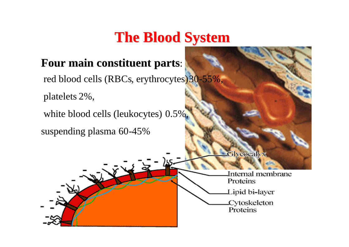
The Blood SystemThe Blood System

FFour main constituent partsour main constituent parts:

red blood cells (RBCs, erythrocytes)30-55%,

white blood cells (leukocytes) 0.5%,

platelets 2%,

suspending plasma 60-45%

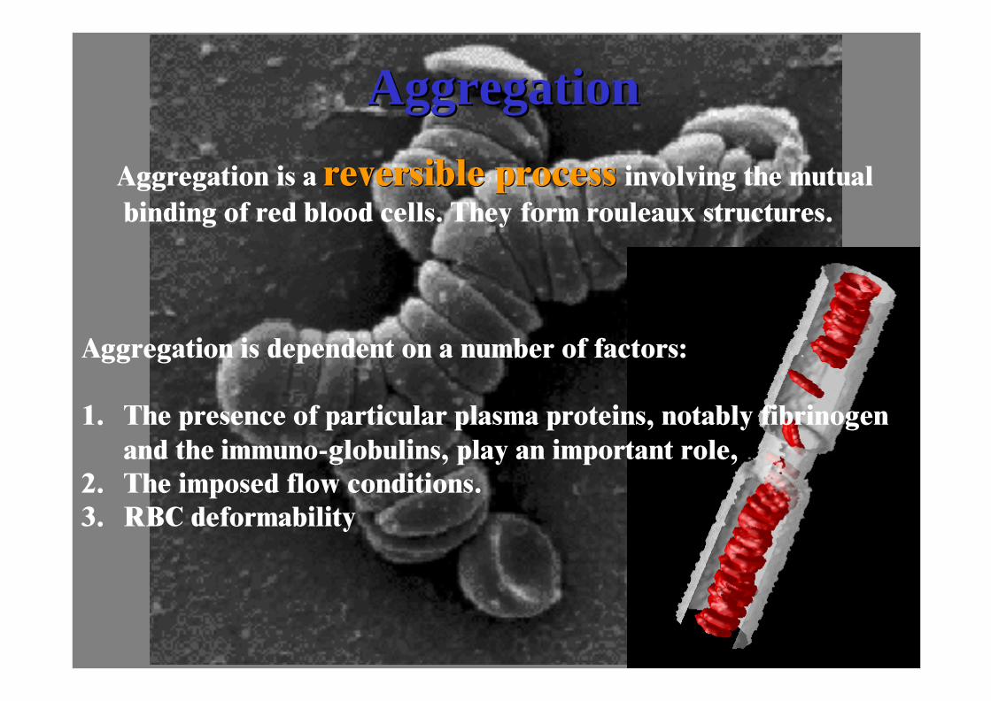
AggregationAggregation

Aggregation is a reversible processreversible process involving the mutual binding of red blood cells. They form rouleaux structures.

Aggregation is dependent on a number of factors:

1. The presence of particular plasma proteins, notably fibrinogen and the immuno-globulins, play an important role,

2. The imposed flow conditions. 3. RBC deformability

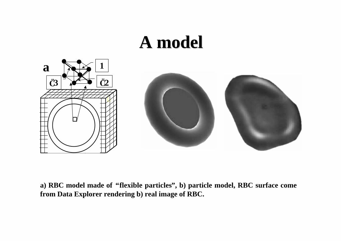
A modelA model

b c

a) RBC model made of “flexible particles”, b) particle model, RBC surface come from Data Explorer rendering b) real image of RBC.

1

√2 √3

a

DamagedDamaged cellscells

Sickle hemoglobin and normal hemoglobin carry the same amount of oxygen.

They differ in the way they flow through the blood vessels. Normal hemoglobin is found in disc-shaped red blood cells that are soft (like a bag of jelly), which enables them to easily flow through small blood vessels. Diseased red blood cells which are sicklesickle--shaped and are hardshaped and are hard(like pieces of wood), often get stuck in small blood vessels and often get stuck in small blood vessels and stop the flow of blood.stop the flow of blood.

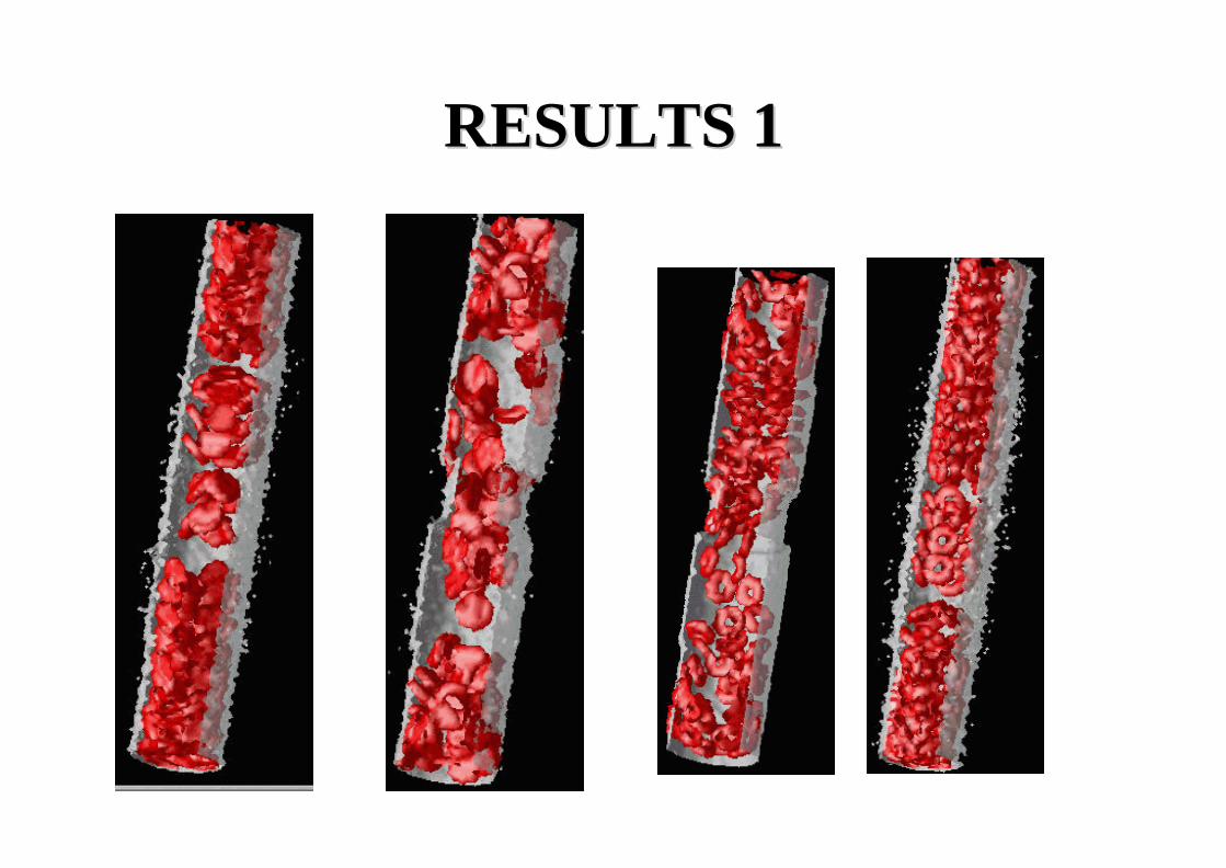
RESULTS 1RESULTS 1

a b

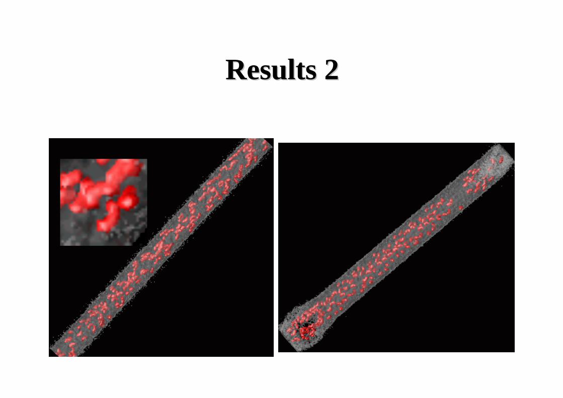
ResultsResults 22

DirectDirect SimulationSimulation MonteMonte--CarloCarlo

A.L. Garcia and F. Balasa method by G.A. Bird

MotivationMotivationWe consider here physical and chemical problems in which a continuum description of a gas is not accurate.

The continuum formulation breaks down when the characteristic length scale in our system is comparable to the mean free path for molecules in the gas.

For air at atmospheric pressure, the mean free path is approximately 50 nm (about the wavelength of visible light) while in the rared upper atmosphere (120 km altitude), the mean free path is several meters. One defines the Knudsen Knudsen numbernumber as Kn = λ/L, where L is the characteristic length scale of the physical system. In general, the continuum description is no longer accurate when

Kn > 1/10.

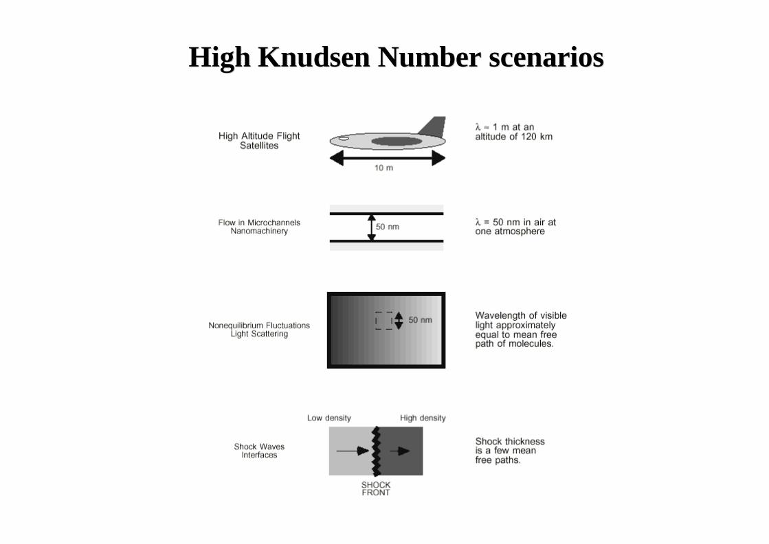
HighHigh KnudsenKnudsen NumberNumber scenariosscenarios

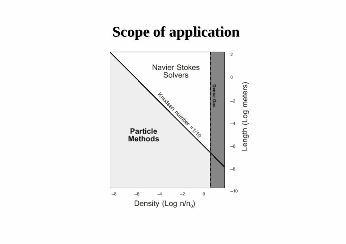
ScopeScope ofof applicationapplication

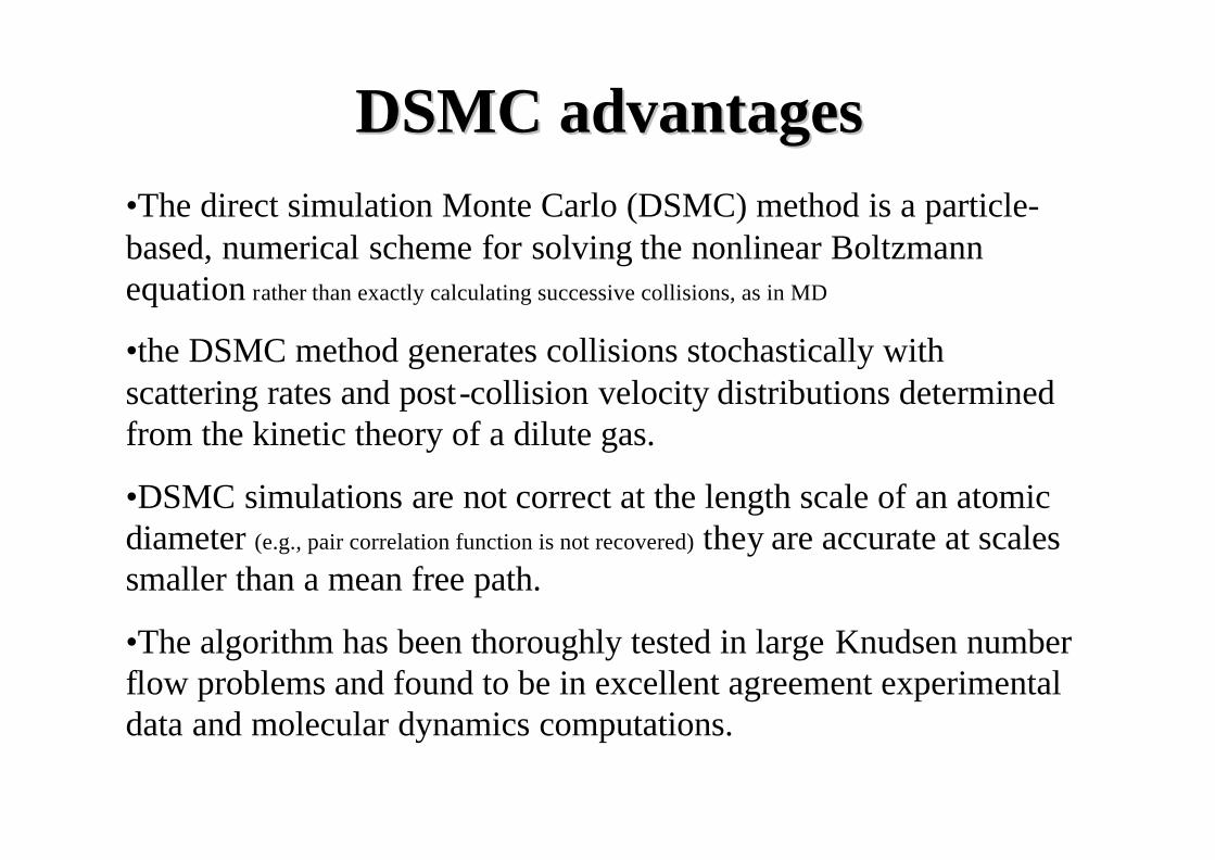
DSMC DSMC advantagesadvantages•The direct simulation Monte Carlo (DSMC) method is a particle-based, numerical scheme for solving the nonlinear Boltzmannequation rather than exactly calculating successive collisions, as in MD

•the DSMC method generates collisions stochastically with scattering rates and post-collision velocity distributions determined from the kinetic theory of a dilute gas.

•DSMC simulations are not correct at the length scale of an atomic diameter (e.g., pair correlation function is not recovered) they are accurate at scales smaller than a mean free path.

•The algorithm has been thoroughly tested in large Knudsen number flow problems and found to be in excellent agreement experimental data and molecular dynamics computations.

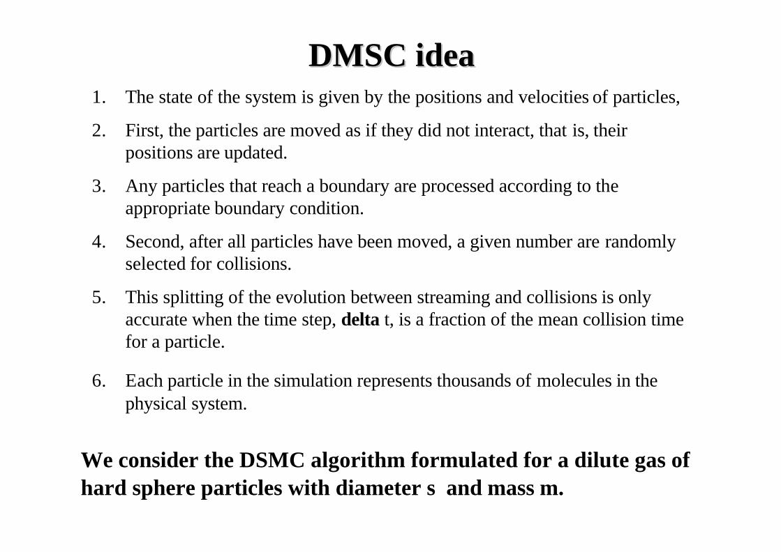
DMSC ideaDMSC idea1. The state of the system is given by the positions and velocities of particles,

2. First, the particles are moved as if they did not interact, that is, their positions are updated.

3. Any particles that reach a boundary are processed according to the appropriate boundary condition.

4. Second, after all particles have been moved, a given number are randomly selected for collisions.

5. This splitting of the evolution between streaming and collisions is only accurate when the time step, delta t, is a fraction of the mean collision time for a particle.

6. Each particle in the simulation represents thousands of molecules in the physical system.

We consider the DSMC algorithm formulated for a dilute gas of hard sphere particles with diameter σ and mass m.

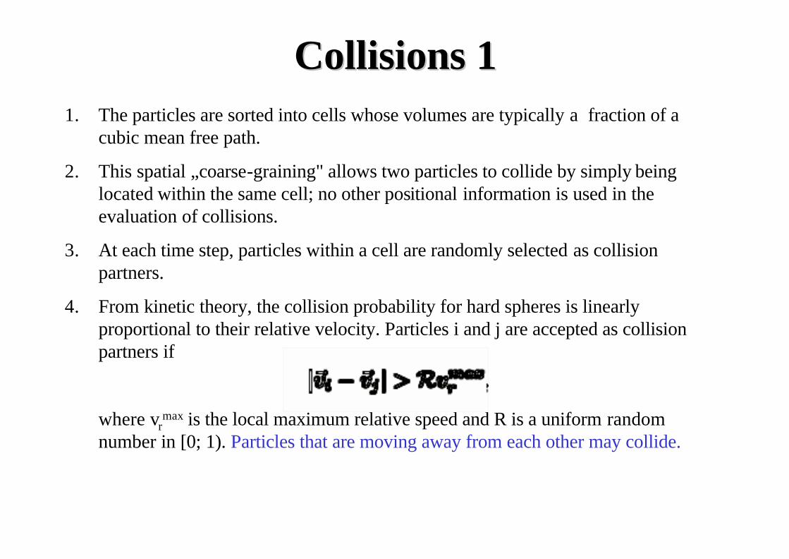
CollisionsCollisions 111. The particles are sorted into cells whose volumes are typically a fraction of a

cubic mean free path.

2. This spatial „coarse-graining" allows two particles to collide by simply being located within the same cell; no other positional information is used in the evaluation of collisions.

3. At each time step, particles within a cell are randomly selected as collision partners.

4. From kinetic theory, the collision probability for hard spheres is linearly proportional to their relative velocity. Particles i and j are accepted as collision partners if

where vrmax is the local maximum relative speed and R is a uniform random

number in [0; 1). Particles that are moving away from each other may collide.

1. Conservation of momentum and energy provide four of the six equations needed to determine the post-collision velocities. The remaining two conditions are selected at random with the assumption that the direction of the post-collision relative velocity is uniformly distributed in the unit sphere. This assumption is exact for hard sphere particles at low densities and has been found to be an excellent approximation in general.

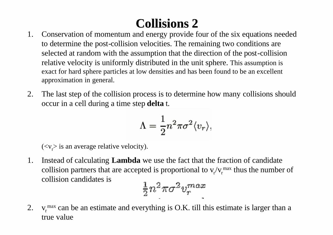
2. The last step of the collision process is to determine how many collisions should occur in a cell during a time step delta t.

(<vr> is an average relative velocity).

1. Instead of calculating Lambda we use the fact that the fraction of candidate collision partners that are accepted is proportional to vr/vr

max thus the number of collision candidates is

2. vrmax can be an estimate and everything is O.K. till this estimate is larger than a

true value

CollisionsCollisions 22

BoundariesBoundaries

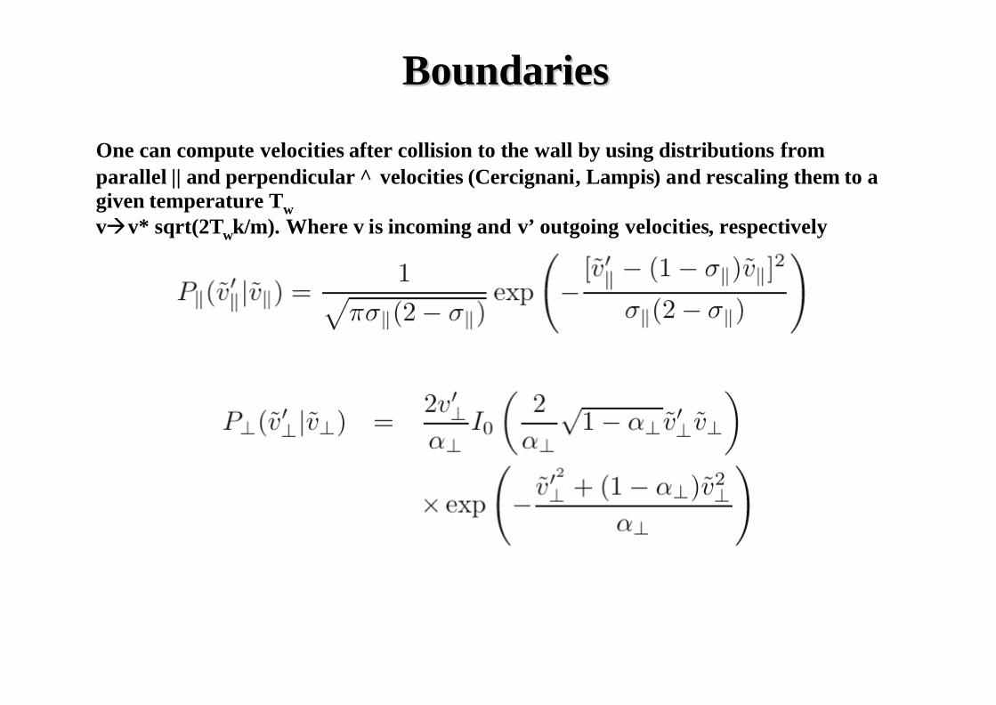
One can compute velocities after collision to the wall by using distributions fromparallel || and perpendicular ⊥ velocities (Cercignani, Lampis) and rescaling them to a given temperature Twvàv* sqrt(2Twk/m). Where v is incoming and v’ outgoing velocities, respectively

StatisticsStatistics andand time time averagesaverages

Temperature can be computed from:

The averages are computed over the cells:

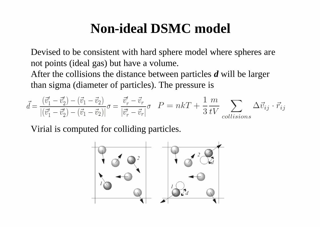
Non-ideal DSMC model

Devised to be consistent with hard sphere model where spheres are not points (ideal gas) but have a volume. After the collisions the distance between particles d will be larger than sigma (diameter of particles). The pressure is

Virial is computed for colliding particles.

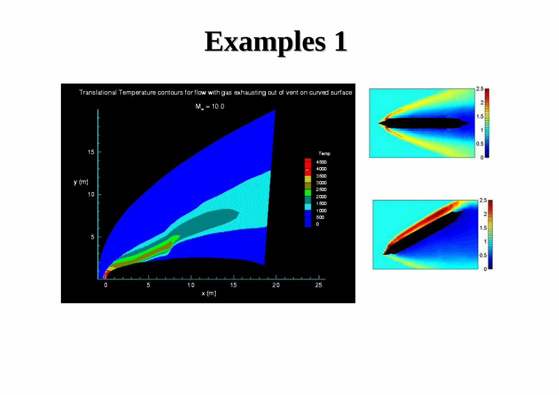
ExamplesExamples 11

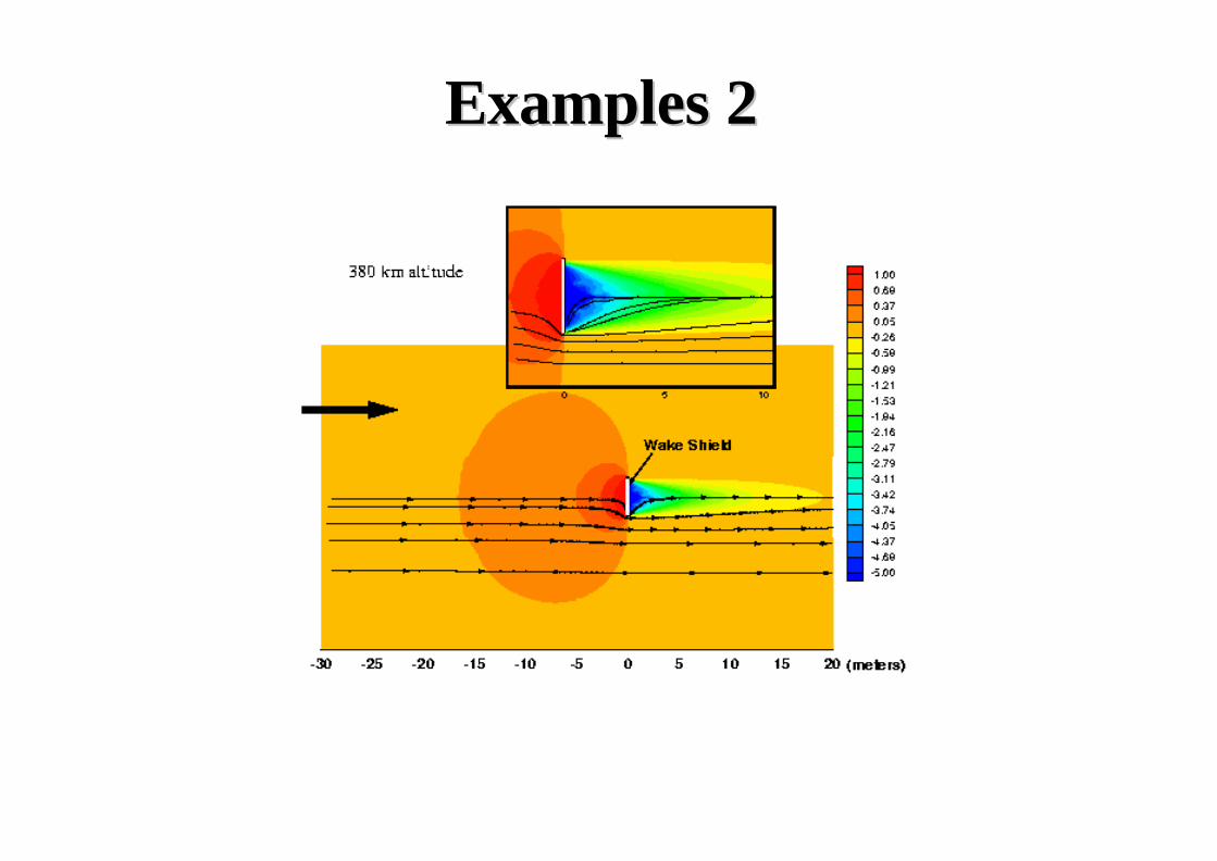
ExamplesExamples 22

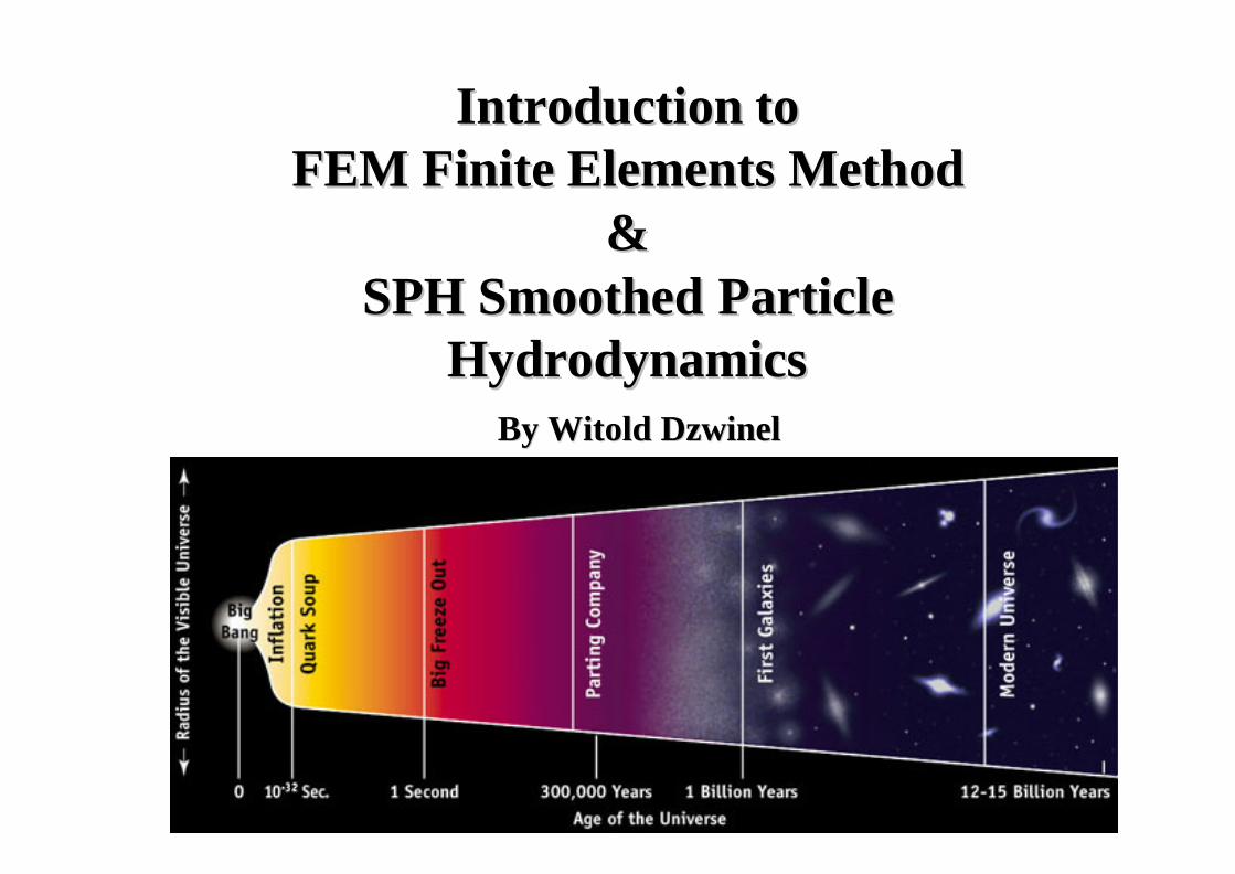
IntroductionIntroduction totoFEM FEM FiniteFinite ElementsElements MethodMethod

& & SPH SPH SmoothedSmoothed ParticleParticle

HydrodynamicsHydrodynamicsBy Witold By Witold DzwinelDzwinel

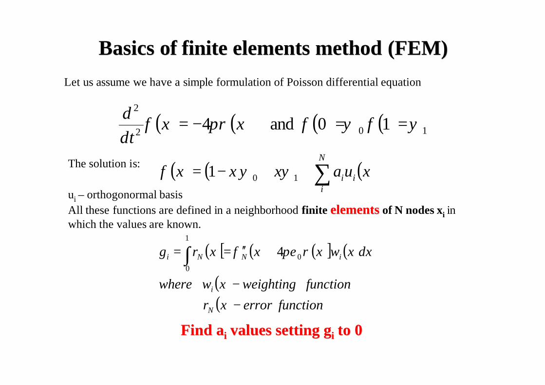
BasicsBasics ofof finitefinite elementselements methodmethod (FEM)(FEM)Let us assume we have a simple formulation of Poisson differential equation

( ) ( ) ( ) ( ) 102

2

1 0 and 4 ψφψφπρφ ==−= xxdtd

The solution is: ( ) ( ) ( )xuaxxx i

N

ii∑++−= 101 ψψφ

ui – orthogonormal basisAll these functions are defined in a neighborhood finite elementselements of N nodes xi inwhich the values are known.

( ) ( ) ( )[ ] ( )

( )( ) functionerrorxr

functionweightingxw where

dxxwxxxrg

N

i

iNNi

4 0

1

0

−−

+′′== ∫ ρπεφ

FindFind aaii valuesvalues settingsetting ggii to 0to 0

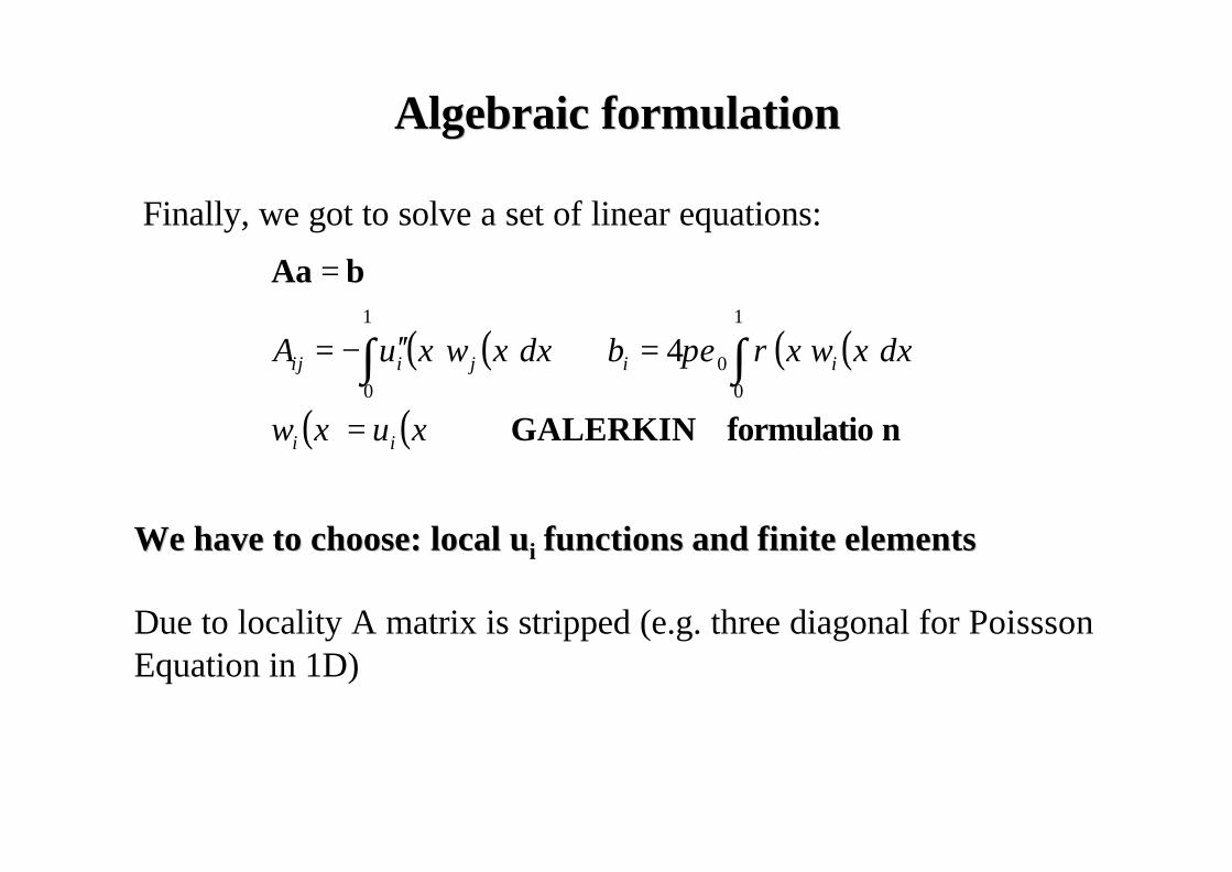
Algebraic formulationAlgebraic formulation

Finally, we got to solve a set of linear equations:

( ) ( ) ( ) ( )

( ) ( ) nformulatioGALERKIN

bAa

4 1

00

1

0

xuxw

dxxwxbdxxwxuA

ii

iijiij

=

=′′−=

=

∫∫ ρπε

We have to choose: local We have to choose: local uuii functions and finite elementsfunctions and finite elements

Due to locality A matrix is stripped (e.g. three diagonal for PoisssonEquation in 1D)

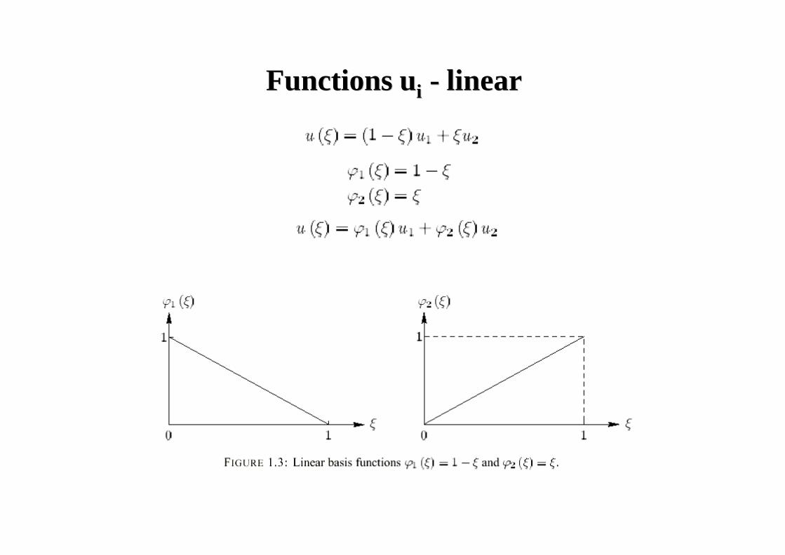
Functions Functions uuii -- linearlinear

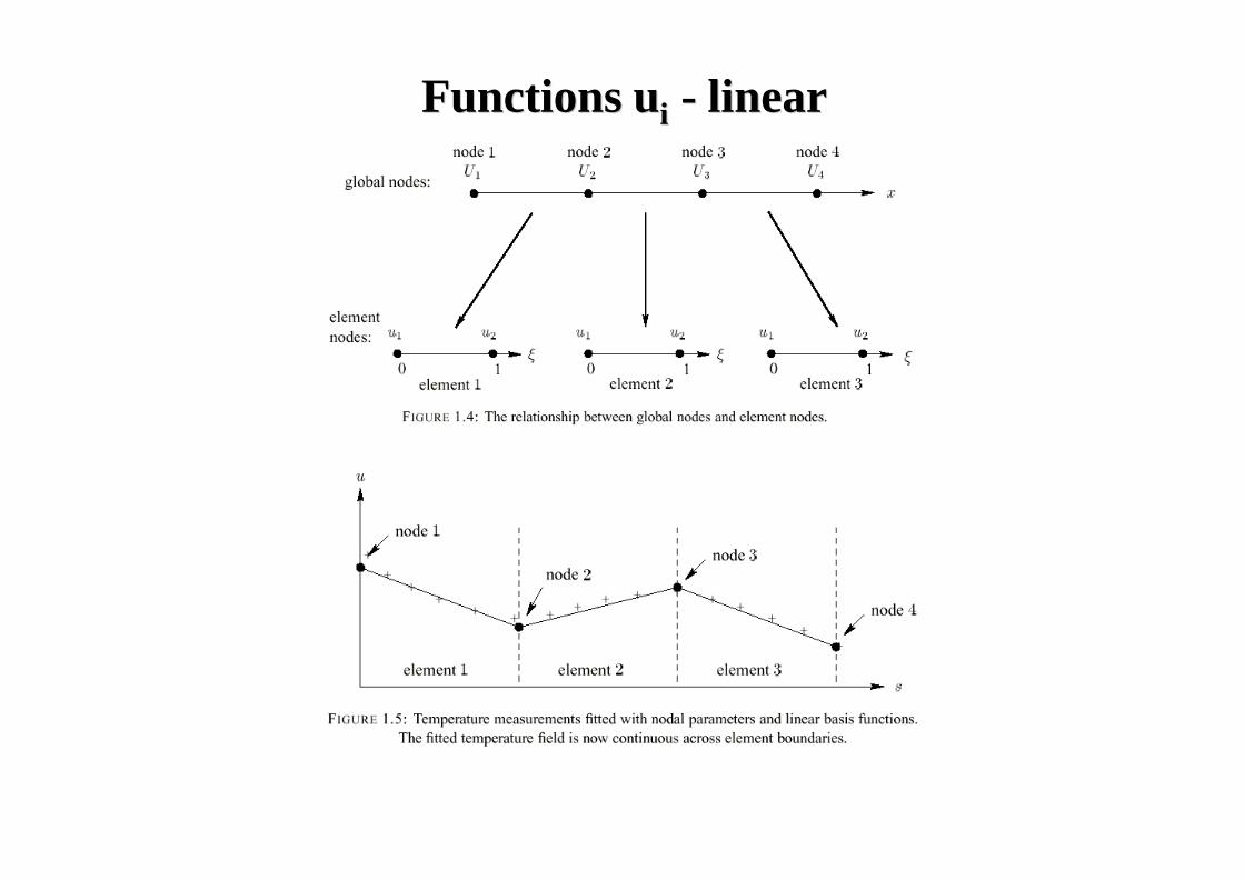
FunctionsFunctions uuii -- linearlinear

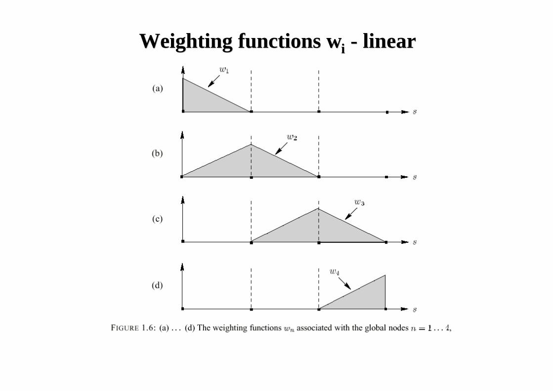
Weighting functions Weighting functions wwii -- linearlinear

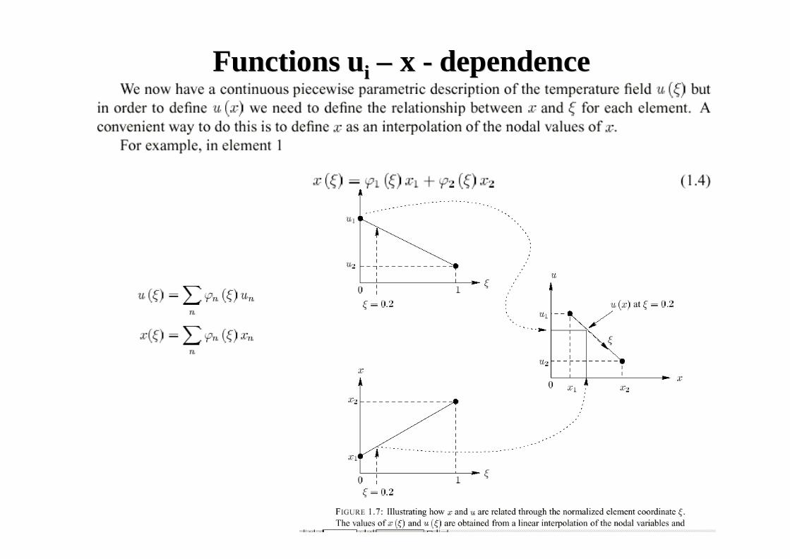
FunctionsFunctions uuii –– x x -- dependencedependence

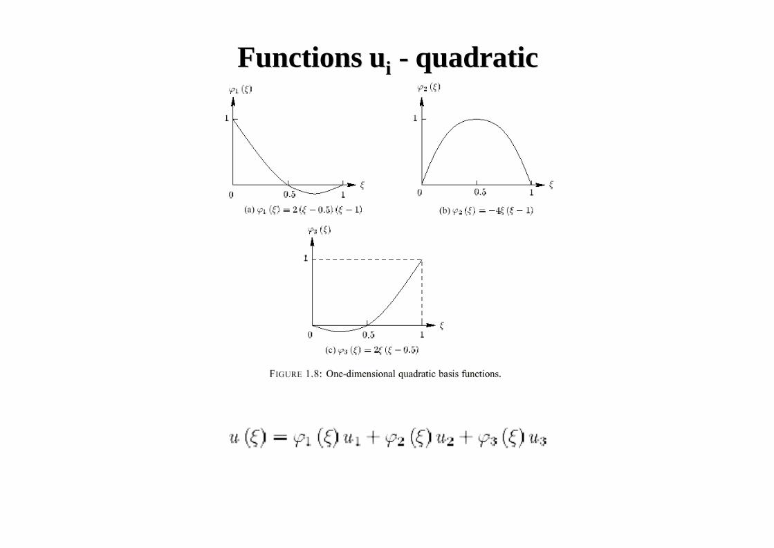
Functions Functions uuii -- quadraticquadratic

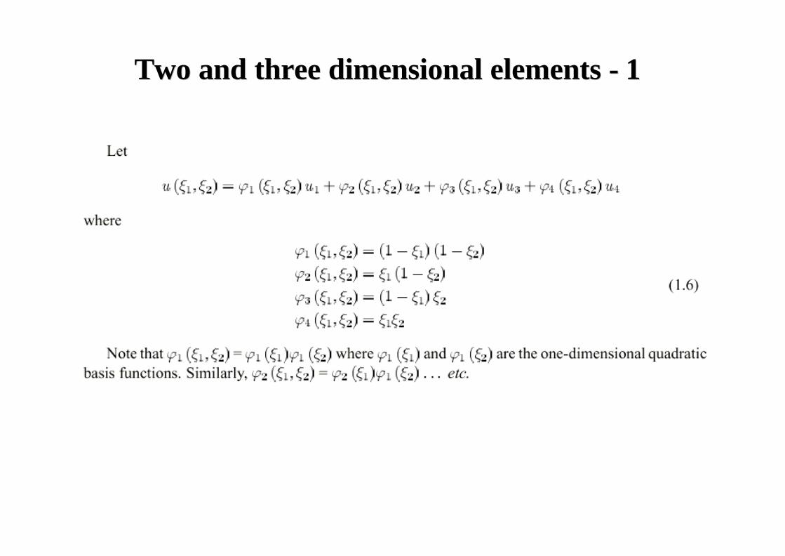
Two and three dimensional elements Two and three dimensional elements -- 11

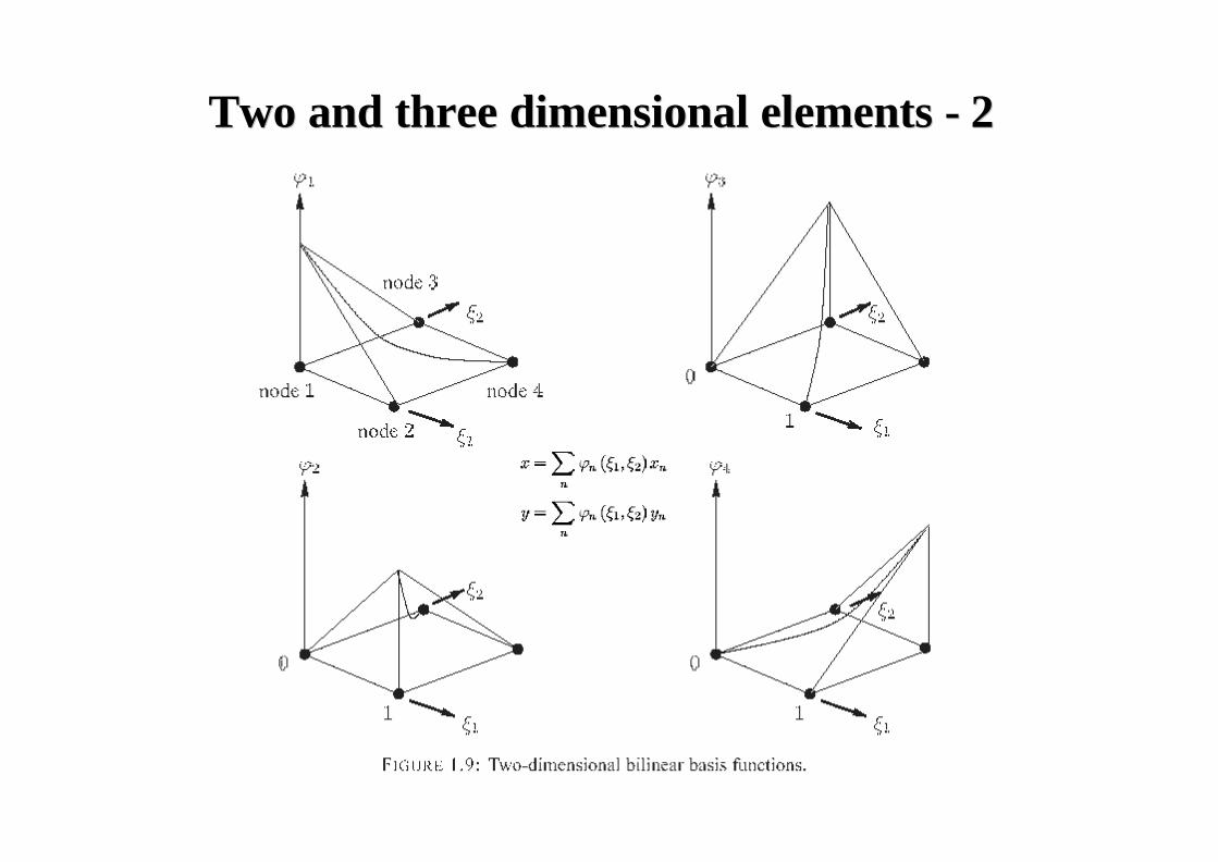
Two and three dimensional elements Two and three dimensional elements -- 22

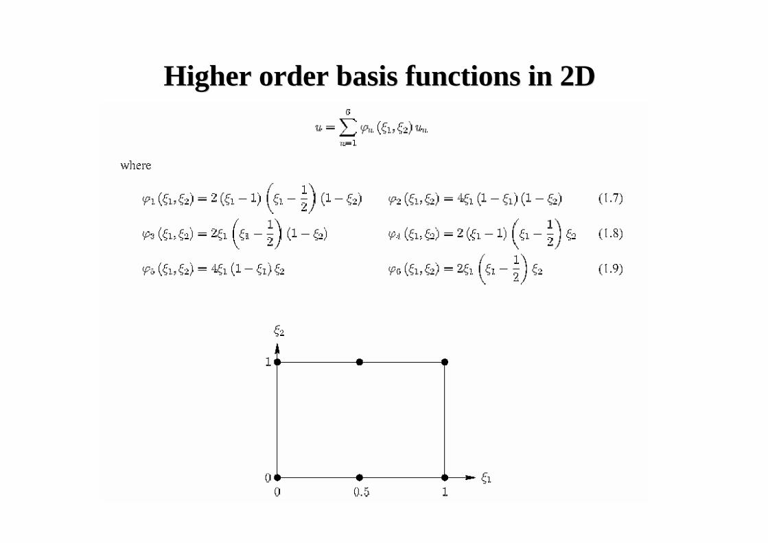
Higher order basis functions in 2DHigher order basis functions in 2D

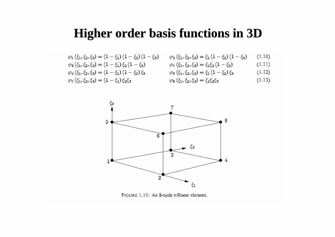
Higher order basis functions in 3DHigher order basis functions in 3D

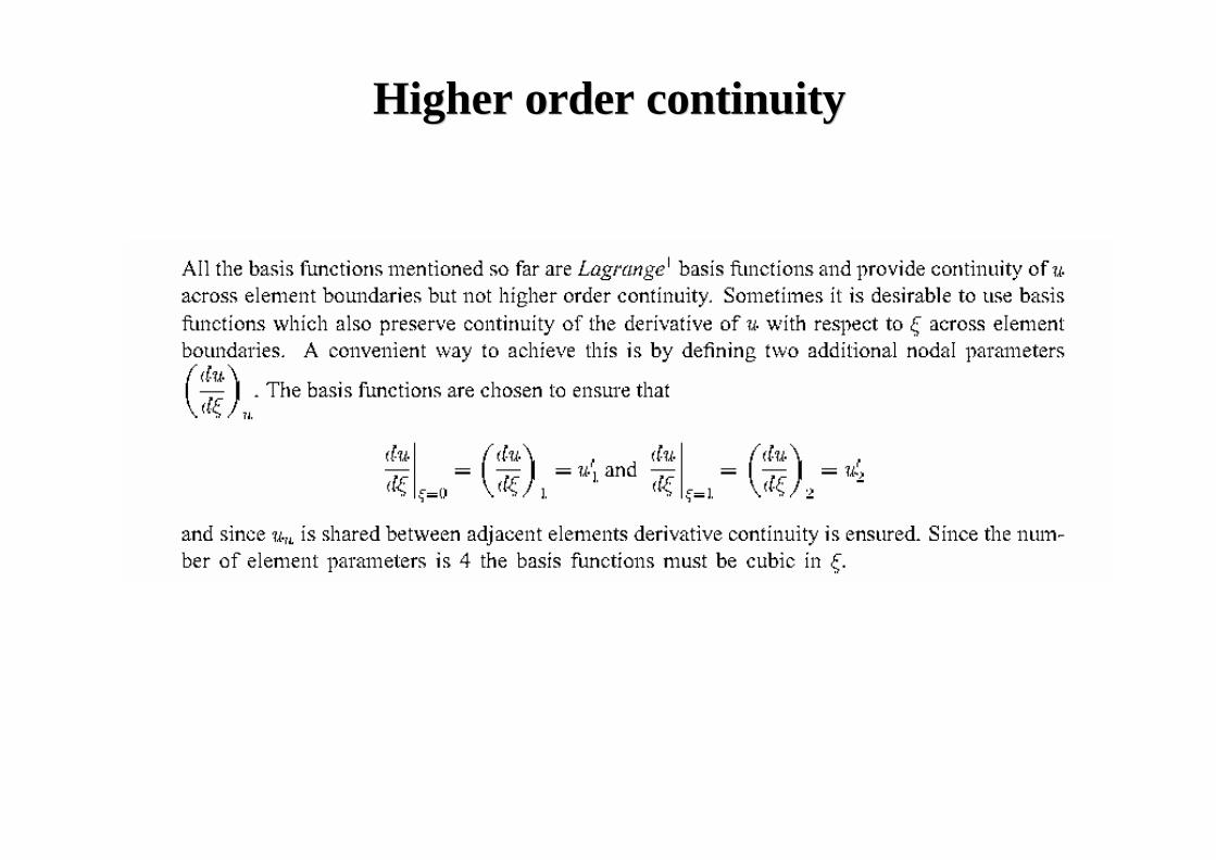
HigherHigher order order continuitycontinuity

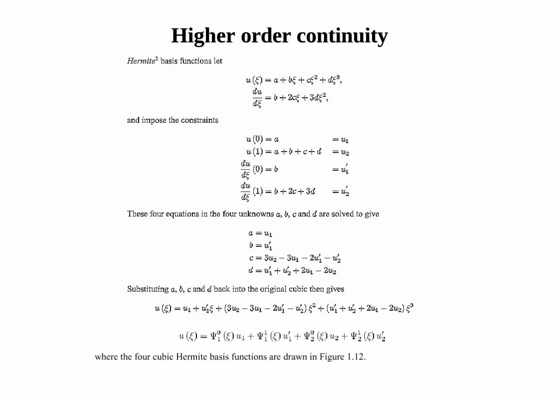
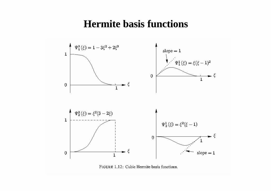
HigherHigher order order continuitycontinuity

HermiteHermite basisbasis functionsfunctions

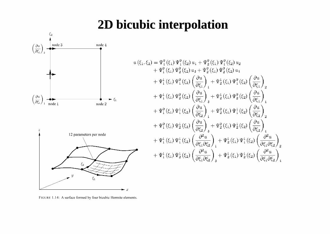
2D 2D bicubicbicubic interpolationinterpolation

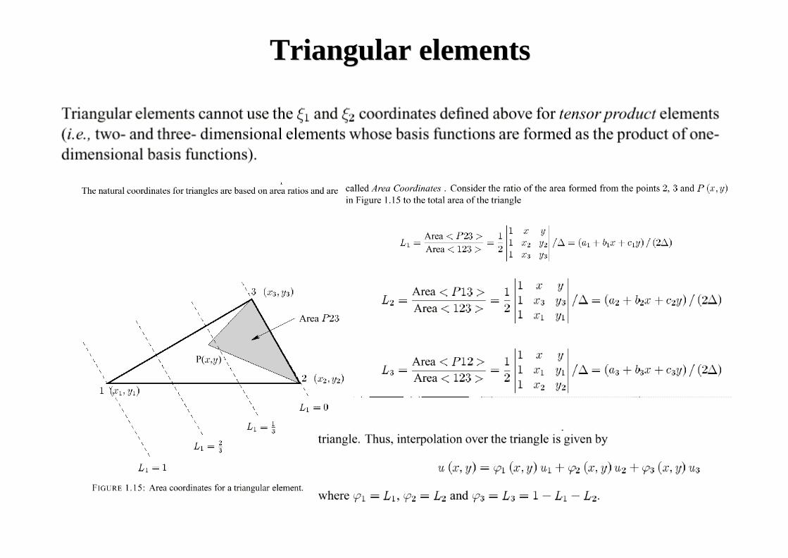
Triangular elementsTriangular elements

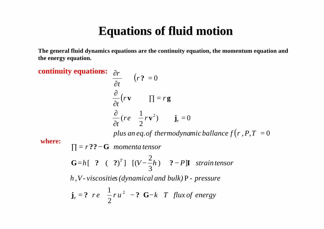
Equations of fluid motionEquations of fluid motionThe general fluid dynamics equations are the continuity equation, the momentum equation and the energy equation.

continuity equations:( )

( )

( ) 0,,

0)21

(

0

2

=

=⋅∇++∂∂

=∏⋅∇+∂∂

=∇+∂∂

TPf ballance micthermodyna of eq. an plust

t

t

e

ρ

ρρε

ρρ

ρρ

jv

gv

?

where:

energy of fluxT

pressurebulk) and (dynamical sviscositie

tensor strainP

tensor momenta

e

T

21

- P -,

])32

[(])([

2 ∇−⋅−

+=

−⋅∇−+∇+∇=

−=∏

κρυρε

ςη

ηςη

ρ

G??j

I???G

G??

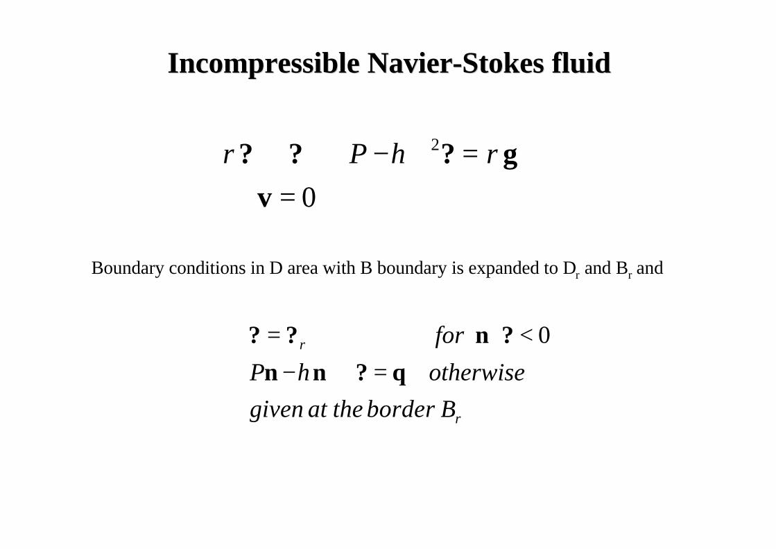
Incompressible Incompressible NavierNavier--Stokes fluidStokes fluid

0

2

=⋅∇=∇−∇+∇⋅

vg??? ρηρ P

Boundary conditions in D area with B boundary is expanded to Dr and Br and

r

r

B border the at givenotherwisePfor

0

q?nn?n??

=∇⋅−<⋅=

η

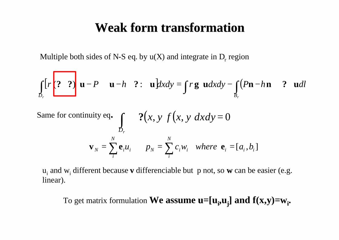
Weak form transformationWeak form transformation

[ ] ( ) dlPdxdydxdyPrr BD

u?nnugu?uu?? ⋅∇⋅−−⋅=∇∇−⋅∇−⋅∇ ∫ ∫∫ ηρηρ :)(

Multiple both sides of N-S eq. by u(X) and integrate in Dr region

Same for continuity eq.. ( ) ( ) 0,, =⋅∇∫ dxdyyxfyxrD

?

],[ iii

N

iiiN

N

iiiN ba wherewcpu === ∑∑ eev

ui and wi different because v v differenciable but p not, so ww can be easier (e.g. linear).

To get matrix formulation We assume uu=[ui,uj] and f(x,y)=wi.

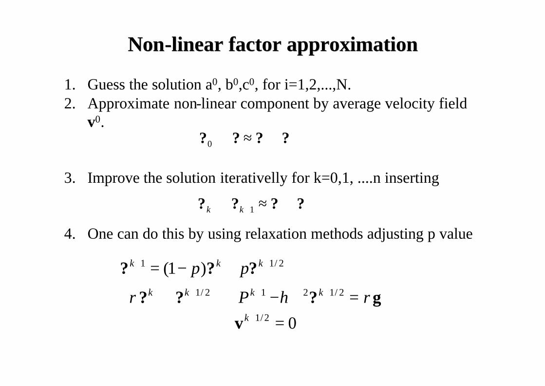
NonNon--linear factor approximationlinear factor approximation

1. Guess the solution a0, b0,c0, for i=1,2,...,N.2. Approximate non-linear component by average velocity field

v0.

3. Improve the solution iterativelly for k=0,1, ....n inserting

4. One can do this by using relaxation methods adjusting p value

???? ∇⋅≈∇⋅0

???? ∇⋅≈∇⋅ +1kk

=⋅∇=∇−∇+∇⋅

+−=

+

+++

++

0

)1(

2/1

2/1212/1

2/11

k

kkkk

kkk

P

pp

vg???

???

ρηρ

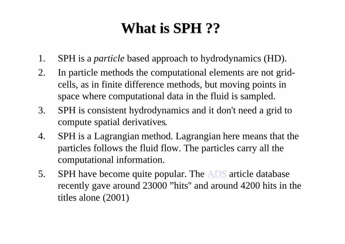
What is SPHWhat is SPH ????

1. SPH is a particle based approach to hydrodynamics (HD). 2. In particle methods the computational elements are not grid-

cells, as in finite difference methods, but moving points in space where computational data in the fluid is sampled.

3. SPH is consistent hydrodynamics and it don't need a grid to compute spatial derivatives.

4. SPH is a Lagrangian method. Lagrangian here means that the particles follows the fluid flow. The particles carry all the computational information.

5. SPH have become quite popular. The ADS article database recently gave around 23000 ”hits'' and around 4200 hits in the titles alone (2001)

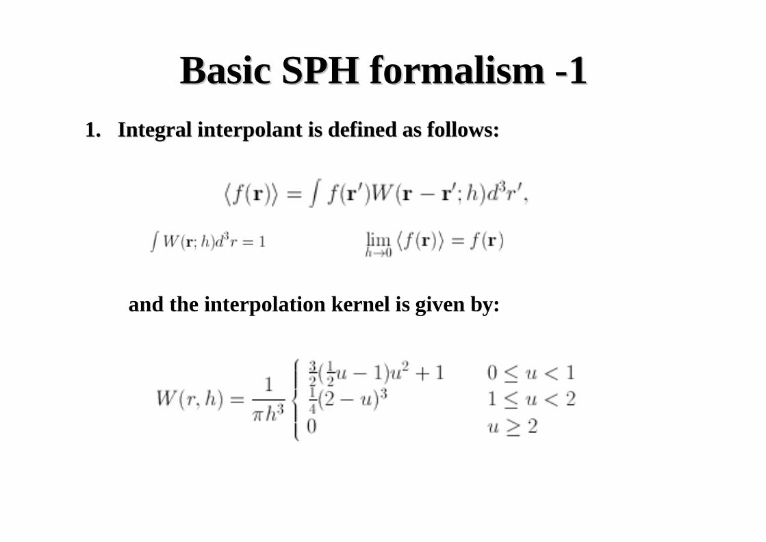
Basic SPH Basic SPH formalismformalism --111.1. Integral Integral interpolantinterpolant is defined as follows:is defined as follows:

and the interpolation kernel is given by:

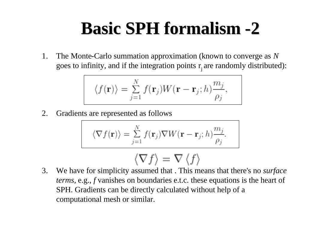
Basic SPH Basic SPH formalismformalism --221. The Monte-Carlo summation approximation (known to converge as N

goes to infinity, and if the integration points rj are randomly distributed):

2. Gradients are represented as follows

3. We have for simplicity assumed that . This means that there's no surface terms, e.g., f vanishes on boundaries e.t.c. these equations is the heart of SPH. Gradients can be directly calculated without help of a computational mesh or similar.

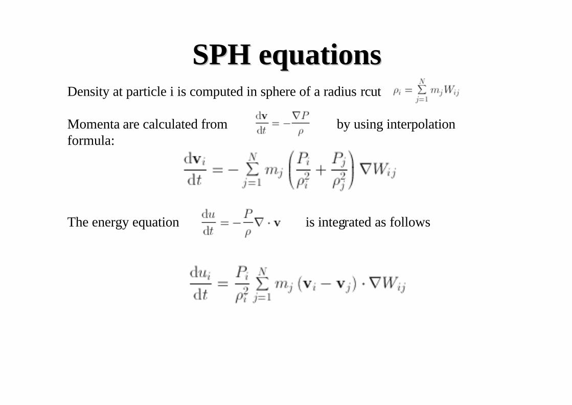
Density at particle i is computed in sphere of a radius rcut

Momenta are calculated from by using interpolation formula:

The energy equation is integrated as follows

SPH SPH equationsequations

Artificial viscosityArtificial viscosity

1. In SPH shocks are handled by introducing artificial viscosity to smear out discontinuities to resolvable scales. Although the SPH kernel smoothing procedure itself ``smoothes'' discontinuities, the particles will still move irregularly across a shock front, and post shock oscillations appear.

2. Artificial viscosity damps irregular motions and the particles move closer to the average velocity in the region. Artificial viscosity pressure terms are usually of two types: bulk viscosity proportional to the divergence of the velocity field, and Von Neumann-Richtmyer viscosity, proportional to its square.

3. where , cij = (ci + cj)/2 is the average sound speed of particle i and j, and

When is SPH When is SPH usefuluseful??

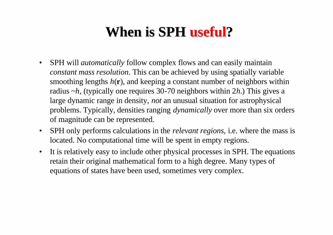
• SPH will automatically follow complex flows and can easily maintain constant mass resolution. This can be achieved by using spatially variable smoothing lengths h(r), and keeping a constant number of neighbors within radius ~h, (typically one requires 30-70 neighbors within 2h.) This gives a large dynamic range in density, not an unusual situation for astrophysical problems. Typically, densities ranging dynamically over more than six orders of magnitude can be represented.

• SPH only performs calculations in the relevant regions, i.e. where the mass is located. No computational time will be spent in empty regions.

• It is relatively easy to include other physical processes in SPH. The equations retain their original mathematical form to a high degree. Many types of equations of states have been used, sometimes very complex.

When is SPH When is SPH usefuluseful??

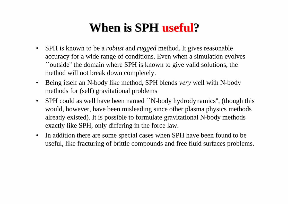
• SPH is known to be a robust and rugged method. It gives reasonable accuracy for a wide range of conditions. Even when a simulation evolves ``outside'' the domain where SPH is known to give valid solutions, the method will not break down completely.

• Being itself an N-body like method, SPH blends very well with N-body methods for (self) gravitational problems

• SPH could as well have been named ``N-body hydrodynamics'', (though this would, however, have been misleading since other plasma physics methods already existed). It is possible to formulate gravitational N-body methods exactly like SPH, only differing in the force law.

• In addition there are some special cases when SPH have been found to be useful, like fracturing of brittle compounds and free fluid surfaces problems.

When is SPH When is SPH notnot useful?useful?• Boundary conditions are usually difficult to implement in SPH. Handling of boundaries

does not come very natural. Special techniques need to be employed, but often these do not fit ``smoothly'' into the method. Typically, it can be difficult to prevent particles from penetrating boundaries. If complicated boundary conditions are central in the problem (like the air flow around an aircraft) SPH is simply not the method of choice.

• Shock phenomena is not the strongest part of SPH. SPH relies on the use of artificial viscosity, in order to resolve shocks. Typical shock resolution is then around three smoothing lengths. State of the art finite difference schemes, like the Piecewise Parabolic Method (PPM), can achieve far better (at comparable resolution). Typically,SPH needs numbers of particles in excess of 10 000, when shocks are present.

• SPH works best if the smoothing lengths are variable, but the resolution will then be highest in high density regions. Low density regions may then be poorly resolved. The transition of sound waves into shocks, as they propagate into a rarefied medium, is an example where SPH would not be suitable.

• In generic SPH spherical kernel functions are used. The distribution of neighbors to a particle should then be roughly isotropic for the interpolation formulae to work properly. This will not be the case if thin (<~h), sheets or disks forms. Although, this is mainly a question of using sufficient resolution (enough many particles), three dimensional SPH does not correctly represent ``two dimensional'' SPH when a computational region contracts to a sheet.

SuperSupernnowa owa explosionexplosion

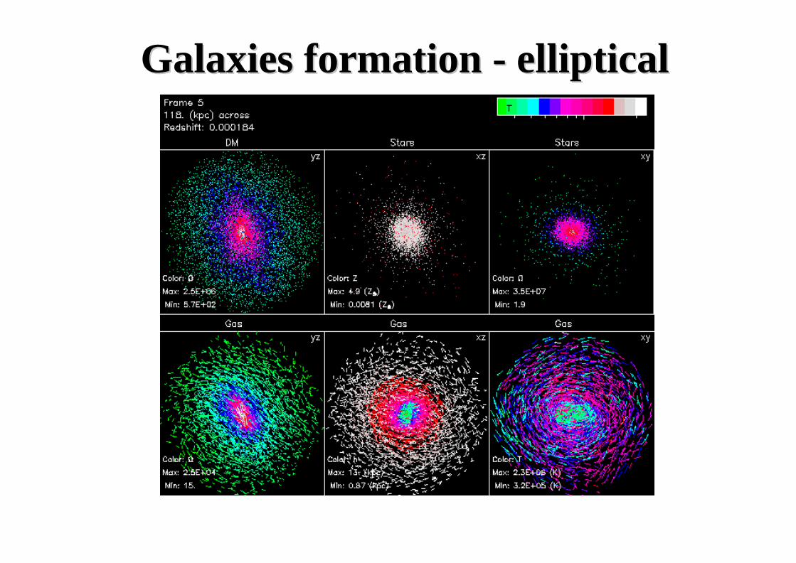
Galaxies formation Galaxies formation -- ellipticalelliptical

Merging of galaxiesMerging of galaxies