forward and inverse problems in the mechanics of soft

rsos.royalsocietypublishing.org

ResearchCite this article: Gazzola M, Dudte LH,McCormick AG, Mahadevan L. 2018 Forwardand inverse problems in the mechanics of softfilaments. R. Soc. open sci. 5: 171628.http://dx.doi.org/10.1098/rsos.171628

Received: 13 October 2017Accepted: 30 April 2018

Subject Category:Engineering

Subject Areas:applied mathematics/mechanics/computational mechanics

Keywords:soft filaments, computational mechanics,Cosserat theory

Author for correspondence:L. Mahadevane-mail: [email protected]

Electronic supplementary material is availableonline at https://doi.org/10.6084/m9.figshare.c.4111496

Forward and inverseproblems in the mechanicsof soft filamentsM. Gazzola1, L. H. Dudte2, A. G. McCormick4 and

L. Mahadevan2,3

1Department of Mechanical Science and Engineering, and National Center forSupercomputing Applications, University of Illinois at Urbana-Champaign, Urbana, IL61801, USA2John A. Paulson School of Engineering and Applied Sciences, and 3Department ofPhysics, Harvard University, Cambridge, MA 02138, USA4Google, Mountain View, CA 94043, USA

LM, 0000-0002-5114-0519

Soft slender structures are ubiquitous in natural and artificialsystems, in active and passive settings and across scales, frompolymers and flagella, to snakes and space tethers. In thispaper, we demonstrate the use of a simple and practicalnumerical implementation based on the Cosserat rod model tosimulate the dynamics of filaments that can bend, twist, stretchand shear while interacting with complex environments viamuscular activity, surface contact, friction and hydrodynamics.We validate our simulations by solving a number of forwardproblems involving the mechanics of passive filaments andcomparing them with known analytical results, and extendthem to study instabilities in stretched and twisted filamentsthat form solenoidal and plectonemic structures. We then studyactive filaments such as snakes and other slender organisms bysolving inverse problems to identify optimal gaits for limblesslocomotion on solid surfaces and in bulk liquids.

1. IntroductionQuasi one-dimensional objects are characterized by having onedimension, the length L, much larger than the others, say theradius r, so that L/r � 1. Relative to three-dimensional objects,this measure of slenderness allows for significant mathematicalsimplification in accurately describing the physical dynamics ofstrings, filaments and rods. It is thus perhaps not surprisingthat the physics of strings has been the subject of intense studyfor centuries [1–10], and indeed their investigation substantiallypredates the birth of three-dimensional elasticity.

Following the pioneering work of Galileo on the bendingof cantilevers, one-dimensional analytical models of beams date

2018 The Authors. Published by the Royal Society under the terms of the Creative CommonsAttribution License http://creativecommons.org/licenses/by/4.0/, which permits unrestricteduse, provided the original author and source are credited.

http://crossmark.crossref.org/dialog/?doi=10.1098/rsos.171628&domain=pdf&date_stamp=2018-06-13

mailto:[email protected]

https://doi.org/10.6084/m9.figshare.c.4111496

https://doi.org/10.6084/m9.figshare.c.4111496

http://orcid.org/0000-0002-5114-0519

2

rsos.royalsocietypublishing.orgR.Soc.opensci.5:171628

................................................back to 1761 when Jakob Bernoulli first introduced the use of differential equations to capture therelationship between geometry and bending resistance in a planar elastica, that is, an elastic curvedeforming in a two-dimensional space. This attempt was then progressively refined by Huygens et al.[11], until Euler presented a full solution of the planar elastica, obtained by minimizing the strain energyand by recognizing the relationships between flexural stiffness and material and geometric properties.Euler also showed the existence of bifurcating solutions in a rod subject to compression, identifying itsfirst buckling mode, while Lagrange formalized the corresponding multi-modal solution [5]. Non-planardeformations of the elastica were first tackled by Kirchhoff [1,6] and Clebsch [2] who envisaged a rod asan assembly of short undeformable straight segments with dynamics determined by contact forces andmoments, leading to three-dimensional configurations. Later, Love [3] approached the problem from aLagrangian perspective characterizing a filament by contiguous cross sections that can rotate relative toeach other, but remain undeformed and perpendicular to the centre line of the rod at all times; in modernparlance this assumption is associated with dynamics on the rotation group SO(3) at every cross section.The corresponding equations of motion capture the ability of the filament to bend and twist, but notshear or stretch. Eventually, the Cosserat brothers [4] relaxed the assumption of inextensibility and cross-section orthogonality to the centre line, deriving a general mathematical framework that accommodatesall six possible degrees of freedom associated with bending, twisting, stretching and shearing, effectivelyformulating dynamics on the full Euclidean group SE(3).

These mathematical foundations [5] prompted a number of discrete computational models [12–16]that allow for the exploration of a range of physical phenomena. These include, for example, the study ofpolymers and DNA [12,17], elastic ribbons and filaments [14,18,19], botanical applications [20,21], wovencloth [22], and tangled hair and fibres [19,23–25]. Because the scaled ratio of the stretching and shearingstiffness to the bending stiffness for slender filaments is L2/r2 � 1, the assumption of inextensibilityand/or unshearability is usually appropriate, justifying the widespread use of the Kirchhoff model inthe aforementioned applications.

Fewer studies have considered, in different flavours, the Cosserat model, mostly to take advantageof relaxed extension and shearing constraints to simplify numerical implementations and to facilitatethe integration of additional physical effects. For example, specialized models including extension andconstitutive laws based on strain rates have been developed for the investigation of viscous threads[15,16,26–30]. Lim and Peskin allow for small numerical shear and axial strain and couple their modelwith an accurate viscous flow solver to investigate fluid–mechanic interactions of ribbons and flagella[31–36]. The graphics software Corde [13] implements a Cosserat-based fast solver for the renderingof looping systems, accounts for (self) contact, operates in the small extension regime and maintainsthe unshearability constraint, showcasing a number of visually impressive and physically plausiblescenarios. Durville [25] introduced a fibre model specialized to efficiently resolve contact-friction effectsin entangled materials. Linn [37] explored an elegant theoretical connection between Cosserat rods andthe differential geometry of framed curves, and numerically tested it on the classic Euler’s Elastica andKirchhoff’s helix problems [38]. Finally, Sonneville [39] presents a geometrically exact finite elementformulation on the Euclidean group SE(3) and verifies it on test cases that do not involve stretchingor environmental effects.

More recently, there has been a need to generalize the model to explain new experimental phenomenasuch as the plectoneme–solenoid transition [40], that has been used as the basis for artificial muscles[41–43]. Additional new technologies such as soft robotics [44,45] are also generating applications forhighly stretchable and shearable elastomeric structures raising the need for methods able to realisticallyhandle these large strains together with a variety of interface and environmental effects. Moreover,the capability to computationally solve both forward [46–49] and inverse problems is emerging asa crucial paradigm to aid the design of novel, more capable soft-robotic prototypes [50,51], as wellas to characterize from an optimality standpoint biophysical phenomena [52–57]. Motivated by theseadvancements and challenges, we use a versatile implementation of the Cosserat model that we validatein a set of physical simulations, and then deploy in the context of inverse design problems to broadenthe spectrum of its potential engineering and biophysical investigations. By taking advantage of theCosserat formalism, and consistently with the full Euclidean group SE(3), we allow for bend, twistand significant shear and stretch [4], and demonstrate the importance of the latter through an exampleinspired by artificial muscle actuation [41,42] in which the transition between plectonemes and solenoidsis crucially enabled by axial extension. Then, moving beyond the passive mechanics of individualfilaments, we account for the interaction between filaments and complex environments with a numberof additional biological and physical features, including muscular activity, self-contact and contact withsolid boundaries, isotropic and anisotropic surface friction and viscous interaction with a fluid. Finally,

3


................................................we demonstrate the capabilities and the robustness of our solver by embedding it in an inverse designcycle for the identification of optimal terrestrial and aquatic limbless locomotion strategies.

The paper is structured as follows. In §2, we review and introduce the mathematical foundationsof the model. In §3, we present the corresponding discrete scheme and validate our implementationagainst a battery of benchmark problems. In §4, we detail the physical and biological enhancements tothe original model, and finally in §5, we showcase the potential of our solver via the study of solenoidsand plectonemes as well as limbless biolocomotion. Mathematical derivations and additional validationtest cases are presented in the appendix.

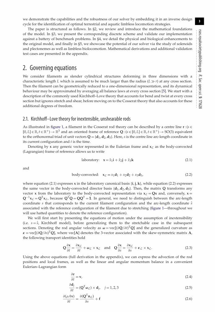
2. Governing equationsWe consider filaments as slender cylindrical structures deforming in three dimensions with acharacteristic length L which is assumed to be much larger than the radius (L � r) at any cross section.Then the filament can be geometrically reduced to a one-dimensional representation, and its dynamicalbehaviour may be approximated by averaging all balance laws at every cross section [5]. We start with adescription of the commonly used Kirchhoff–Love theory that accounts for bend and twist at every crosssection but ignores stretch and shear, before moving on to the Cosserat theory that also accounts for theseadditional degrees of freedom.

2.1. Kirchhoff–Love theory for inextensible, unshearable rodsAs illustrated in figure 1, a filament in the Cosserat rod theory can be described by a centre line r : (s ∈[0, L] ∈ R, t ∈ R

+) → R3 and an oriented frame of reference Q : (s ∈ [0, L] ∈ R, t ∈ R

+) → SO(3) equivalentto the orthonormal triad of unit vectors Q = {d1, d2, d3}. Here, s is the centre line arc-length coordinate inits current configuration and t is the time.

Denoting by x any generic vector represented in the Eulerian frame and xL as the body-convected(Lagrangian) frame of reference allows us to write

laboratory: x = x1i + x2j + x3k (2.1)

and

body-convected: xL = x1d1 + x2d2 + x3d3, (2.2)

where equation (2.1) expresses x in the laboratory canonical basis {i, j, k}, while equation (2.2) expressesthe same vector in the body-convected director basis {d1, d2, d3}. Then, the matrix Q transforms anyvector x from the laboratory to the body-convected representation via xL = Qx and, conversely, x =Q−1xL = QTxL, because QTQ = QQT = 111. In general, we need to distinguish between the arc-lengthcoordinate s that corresponds to the current filament configuration and the arc-length coordinate sassociated with the reference configuration of the filament due to stretching (figure 1—throughout wewill use hatted quantities to denote the reference configuration).

We will first start by presenting the equations of motion under the assumption of inextensibility(i.e. s = s, Kirchhoff model), before generalizing them to the stretchable case in the subsequentsections. Denoting the rod angular velocity as ω = vec[(∂Q/∂t)TQ] and the generalized curvature asκ = vec[(∂Q/∂s)TQ], where vec[A] denotes the 3-vector associated with the skew-symmetric matrix A,the following transport identities hold

Q∂x∂t

= ∂xL∂t

+ ωL × xL and Q∂x∂s

= ∂xL∂s

+ κL × xL. (2.3)

Using the above equations (full derivation in the appendix), we can express the advection of the rodpositions and local frames, as well as the linear and angular momentum balance in a convenientEulerian–Lagrangian form

∂r∂t

= v, (2.4)

∂dj

∂t= (QTωL) × dj, j = 1, 2, 3 (2.5)

∂(ρAv)∂t

= ∂(QTnL)∂s

+ f (2.6)

4


................................................e =

dsds

k

ij

rn (s)

(s) (s + ds)

n (s + ds)

ets

s s

d1

d2

d3 Q = d1d2d3

c

f

n (s)

(s) ((s c

f

Figure 1. The Cosserat rodmodel. A filament deforming in the three-dimensional space is represented by a centre-line coordinate r and amaterial frame characterized by the orthonormal triad {d1, d2, d3}. The corresponding orthogonal rotationmatrixQwith row entries d1,d2, d3 transforms a vector x from the laboratory canonical basis {i, j, k} to the material frame of reference {d1, d2, d3} so that xL = Qxand vice versa x= QTxL. If extension or compression is allowed, the current filament configuration arc-length smay no longer coincidewith the rest reference arc-length s. This is captured via the scalar dilatation field e= ds/ds. Moreover, to account for shear we allow thetriad {d1, d2, d3} to detach from the unit tangent vector t so that d3 �= t (we recall that the condition d3 = t and e= 1 correspond tothe Kirchhoff constraint for unshearable and inextensible rods, and implies thatσ = et − d3 = 0). The dynamics of the centre line andthematerial frame is determined at each cross section by the internal force and torque resultants,n andτ . External loads are representedvia the force f and couple c line densities.

Table 1. Constitutive laws. The generalized curvatureκL is associatedwith the bendingκ1,κ2 about the principal directions (d1,d2) andthe twistκ3 about the longitudinal one (d3), whileσL = Q(et − d3) is associatedwith the shearsσ1,σ2 along the principal directions(d1, d2) and the axial extensional or compression σ3 along the longitudinal one (d3). The material properties of the rod are capturedthrough the Young’s (E) and shear (G) moduli, while its geometric properties are accounted for via the cross-sectional area A, the secondmoment of inertia I and the constant αc = 4

3 for circular cross sections [58]. The diagonal entries of the bending/twist B ∈ R3×3 and

shear/stretch S ∈ R3×3 matrices are, respectively, (B1, B2, B3) and (S1, S2, S3). Pre-strains are modelled via the intrinsic curvature/twist

κ oL and shear/stretchσ o

L.

deformation modes strains rigidities loads

bending about d1 κ1 B1 = EI1 τ1 = B1(κ1 − κ o1 ). . . . . . . . . . . . . . . . . . . . . . . . . . . . . . . . . . . . . . . . . . . . . . . . . . . . . . . . . . . . . . . . . . . . . . . . . . . . . . . . . . . . . . . . . . . . . . . . . . . . . . . . . . . . . . . . . . . . . . . . . . . . . . . . . . . . . . . . . . . . . . . . . . . . . . . . . . . . . . . . . . . . . . . . . . . . . . . . . . . . . . . . . . . . . . . . . . . . . . . . . . . . . . . . . . . . . . . . .

bending about d2 κ2 B2 = EI2 τ2 = B2(κ2 − κ o2 ). . . . . . . . . . . . . . . . . . . . . . . . . . . . . . . . . . . . . . . . . . . . . . . . . . . . . . . . . . . . . . . . . . . . . . . . . . . . . . . . . . . . . . . . . . . . . . . . . . . . . . . . . . . . . . . . . . . . . . . . . . . . . . . . . . . . . . . . . . . . . . . . . . . . . . . . . . . . . . . . . . . . . . . . . . . . . . . . . . . . . . . . . . . . . . . . . . . . . . . . . . . . . . . . . . . . . . . . .

twist about d3 κ3 B3 = GI3 τ3 = B3(κ3 − κ o3 ). . . . . . . . . . . . . . . . . . . . . . . . . . . . . . . . . . . . . . . . . . . . . . . . . . . . . . . . . . . . . . . . . . . . . . . . . . . . . . . . . . . . . . . . . . . . . . . . . . . . . . . . . . . . . . . . . . . . . . . . . . . . . . . . . . . . . . . . . . . . . . . . . . . . . . . . . . . . . . . . . . . . . . . . . . . . . . . . . . . . . . . . . . . . . . . . . . . . . . . . . . . . . . . . . . . . . . . . .

shear along d1 σ1 S1 = αcGA n1 = S1(σ1 − σ o1 ). . . . . . . . . . . . . . . . . . . . . . . . . . . . . . . . . . . . . . . . . . . . . . . . . . . . . . . . . . . . . . . . . . . . . . . . . . . . . . . . . . . . . . . . . . . . . . . . . . . . . . . . . . . . . . . . . . . . . . . . . . . . . . . . . . . . . . . . . . . . . . . . . . . . . . . . . . . . . . . . . . . . . . . . . . . . . . . . . . . . . . . . . . . . . . . . . . . . . . . . . . . . . . . . . . . . . . . . .

shear along d2 σ2 S2 = αcGA n2 = S2(σ2 − σ o2 ). . . . . . . . . . . . . . . . . . . . . . . . . . . . . . . . . . . . . . . . . . . . . . . . . . . . . . . . . . . . . . . . . . . . . . . . . . . . . . . . . . . . . . . . . . . . . . . . . . . . . . . . . . . . . . . . . . . . . . . . . . . . . . . . . . . . . . . . . . . . . . . . . . . . . . . . . . . . . . . . . . . . . . . . . . . . . . . . . . . . . . . . . . . . . . . . . . . . . . . . . . . . . . . . . . . . . . . . .

stretch along d3 σ3 S3 = EA n3 = S3(σ3 − σ o3 ). . . . . . . . . . . . . . . . . . . . . . . . . . . . . . . . . . . . . . . . . . . . . . . . . . . . . . . . . . . . . . . . . . . . . . . . . . . . . . . . . . . . . . . . . . . . . . . . . . . . . . . . . . . . . . . . . . . . . . . . . . . . . . . . . . . . . . . . . . . . . . . . . . . . . . . . . . . . . . . . . . . . . . . . . . . . . . . . . . . . . . . . . . . . . . . . . . . . . . . . . . . . . . . . . . . . . . . . .

and∂(ρIωL)∂t

= ∂τL∂s

+ κL × τL + Q∂r∂s

× nL + (ρIωL) × ωL + cL, (2.7)

where ρ is the constant material density, A is the cross-sectional area, v is the velocity, nL and τL are,respectively, the internal force and couple resultants, f and c are external body force and torque linedensities, and the tensor I is the second area moment of inertia (throughout this study we assume circularcross sections; see the appendix).

To close the above system of equations (2.4)–(2.7) and determine the dynamics of the rod, it isnecessary to specify the form of the internal forces and torques generated in response to bend and twist,corresponding to the 3 d.f. at every cross section. The strains are defined as the relative local deformationsof the rod with respect to its natural strain-free reference configuration. Bending and twisting strainsare associated with the spatial derivatives of the material frame director field {d1, d2, d3} and arecharacterized by the generalized curvature. Specifically, the components of the curvature projectedalong the directors (κL = κ1d1 + κ2d2 + κ3d3) coincide with bending (κ1, κ2) and twist (κ3) strains in thematerial frame (table 1).

5


................................................We assume a perfectly elastic material so that the stress–strain relations are linear. Integration of the

torque densities over the cross-sectional area A yields the bending and twist rigidities (table 1), so thatthe resultant torque–curvature relations can be generically expressed in vectorial notation as

τL = B(κL − κoL), (2.8)

where B ∈ R3×3 = diag(B1, B2, B3) is the bend/twist stiffness matrix, with B1 the flexural rigidity about

d1, B2 the flexural rigidity about d2 and B3 the twist rigidity about d3. Here, the vector κoL characterizes

the intrinsic curvatures of a filament that in its stress-free state is not straight. We wish to emphasize herethat the constitutive laws are most simply expressed in a local Lagrangian form; hence the use of κL andnot κ .

The Kirchhoff rod is defined by the additional assumption that there is no axial extension orcompression or shear strain. Then the arc-length s coincides with s at all times, and the tangent to thecentre line is also normal to the cross section, so that t = d3 [5]. This implies that nL serves as a Lagrangemultiplier, and that the torque-curvature relations of equation (2.8) are linear.

This completes the formulation of the equations of motion for the Kirchhoff rod, and when combinedwith boundary conditions suffices to have a well-posed initial boundary value problem. For the generalstretchable and shearable case, all geometric quantities (A, I, κL, etc.) must be rescaled appropriately, asaddressed in the following sections.

2.2. Cosserat theory of stretchable and shearable filamentsIn the general case of soft filaments, at every cross section we also wish to capture transverse shear andaxial strains in addition to bending and twisting. As we wish to account for all six deformation modesassociated with the 6 d.f. at each cross section along the rod, we must augment the Kirchhoff descriptionof the previous section and add three more constitutive laws to define the local stress resultants nL.In fact, they are no longer defined as Lagrange multipliers that enforce the condition of inextensibilityand unshearability, i.e. we now must allow t �= d3. We note that this not only enables the model ofequations (2.4)–(2.7) to capture a richer set of physical phenomena, but also significantly simplifies itsnumerical treatment (Lagrange multipliers no longer needed), rendering this model both flexible andrelatively straightforward to implement.

The shear and axial strains are associated with the deviations between the unit vector perpendicular tothe cross section and the tangent to the centre line, and thus may be expressed in terms of the derivativesof the centre line coordinate r. In the material frame of reference, we characterize these strains by thevector σ (figure 1) which then takes the form

σL = Q(∂r∂ s

− d3

)= Q(et − d3). (2.9)

Here, the scalar field e(s, t) = ds/ds expresses the local stretching or compression ratio (figure 1) relativeto the rest reference configuration (s) and t is the unit tangent vector.

Whenever the filament undergoes axial stretching or compression the corresponding infinitesimalelements deform and all related geometric quantities are affected. By assuming that the material isincompressible and that the cross sections retain their circular shapes at all times, we can convenientlyexpress the governing equations with respect to the rest reference configuration of the filament (denotedby a hat) in terms of the local dilatation e(s, t). Then, the following relations hold:

ds = e · ds, A = Ae

, I = Ie2 , B = B

e2 , S = Se

and κL = κLe

. (2.10)

As with the Kirchhoff rod, assuming a linear material constitutive law implies linear stress–strainrelations. Integration of the stress and couple densities over the cross-sectional area A yields both therigidities associated with axial extension and shear (table 1), so that the resultant load–strain relations canbe generically expressed in vectorial notation as

nL = S(σL − σ oL), (2.11)

where S ∈ R3×3 = diag(S1, S2, S3) is the shear/stretch stiffness matrix, with S1 the shearing rigidity along

d1, S2 the shearing rigidity along d2 and S3 the axial rigidity along d3. Here, as with the Kirchhoff rod,

6


................................................the vector σ o

L corresponds to the intrinsic shear and stretch, and must be accounted for in the case ofstress-free, non-trivial shapes. Although the intrinsic strains κo

L, σ oL are implemented in our solver to

account for pre-strained configurations, to simplify the notation in the remaining text, we will assumethat the filament is intrinsically straight in a stress-free state, so that σ o

L = κoL = 0.

The rigidities associated with bending, twisting, stretching and shearing are specified in table 1, andcan be expressed as the product of a material component, represented by the Young’s (E) and shear(G) moduli, and a geometric component represented by A, I and the constant αc = 4

3 for circular crosssections [58]. We note that the rigidity matrices B and S are assumed to be diagonal throughout thisstudy, although off-diagonal entries can be easily accommodated to model anisotropic materials such ascomposite elements. In general, this mathematical formulation can be extended to tackle a richer set ofphysical problems including viscous threads [15,16], magnetic filaments [59], etc., by simply modifyingthe entries of B and S and introducing time-dependent constitutive laws wherein τL(κL, ∂tκL) andnL(σL, ∂tσL), as for example in [15]. We also emphasize here that in the case of stretchable rods, Aand I are no longer constant, rendering the load–strain relations nonlinear (equations (2.8) and (2.11)),even though the stress–strain relations remain linear. This is consistent with the modelling of hyperelasticmaterials such as rubbers, silicones and biological tissues and therefore in line with targeted soft roboticapplications. Indeed, the combination of linear stress–strain constitutive models with the geometricalrescaling by e leads to a reasonable approximation of Neo-Hookean [60] and Mooney–Rivlin models[61,62] (especially tailored to hyperelastic solids) over a compression/extension range up to 30%. See theappendix for a quantitative comparison in the axial stretch case.

Having generalized the constitutive relations to account for filament stretchiness and shearability, wenow generalize the equations of motion for this case. Multiplying both sides of equations (2.6) and (2.7)by ds and substituting the above identities together with the constitutive laws of equation (2.11) intoequations (2.4)–(2.7) yields the final system

∂r∂t

= v, (2.12)

∂dj

∂t= (QTωL) × dj, j = 1, 2, 3 (2.13)

dm · ∂2r∂t2 = ∂

∂ s

(QTSσL

e

)ds

︸︷︷︸shear/stretch internal force

+ F︸︷︷︸external force

(2.14)

anddJe

· ∂ωL∂t

= ∂

∂ s

(BκL

e3

)ds + κL × BκL

e3 ds

︸︷︷︸bend/twist internal couple

+ (Qt × SσL) ds︸︷︷︸shear/stretch internal couple

+(

dJ · ωLe

)× ωL︸︷︷︸

Lagrangian transport

+ dJωLe2 · ∂e

∂t︸︷︷︸unsteady dilatation

+ CL︸︷︷︸external couple

, (2.15)

where dm = ρA ds = ρA ds is the infinitesimal mass element, and dJ = ρ I ds is the infinitesimal masssecond moment of inertia. We note that the left-hand side and the unsteady dilatation term ofequation (2.15) arise from the expansion of the original rescaled angular momentum dJ · ∂t(ωL/e) viathe chain rule. We also note that the external force and couple are defined as F = ef ds and CL = ecL ds(with f and cL the force and torque line densities, respectively) so as to account for the dependence on e.

Combined with some initial and boundary conditions, equations (2.12)–(2.15) express the dynamicsand kinematics of the Cosserat rod with respect to its initial rest configuration, in a form suitable to bediscretized as described in §3.

3. Numerical methodTo derive the numerical method for the time evolution of a filament in analogy with the continuum modelof §2, we first recall a few useful definitions for effectively implementing rotations. We then present thespatially discretized model of the rod, and the time discretization approach employed to evolve thegoverning equations.

7


................................................Qi

di2

di3

ri

ri+1

ri+3

ri+2

eiti

ei = —

mi

mi+1

�i

�i�i

si

Qi+1

Qi+2

di1

Figure 2. Discretization model. A discrete filament is represented through a set of vertices r(t)i=1,...,N+1 and a set of material framesQi(t)= {di1, di2, di3, }i=1,...,N . Two consecutive vertices define an edge of length �i along the tangent unit vector ti . The dilatation isdefined as ei = �i/�i , where �i is the edge rest length. The vector σ i = eiti − di3 represents the discrete shear and axial strains.Themassmr of the filament is discretized in pointwise concentratedmassesmi=1,...,n+1 at the locations ri for the purpose of advecting thevertices in time. For the evolution of Qi in time, we consider instead the mass second moment of inertia Ji=1,...,n associated withthe cylindrical elements depicted in blue.

3.1. RotationsBending and twisting deformations of a filament involve rotations of its material frame Q in space andtime. To numerically simulate the rod, it is critical to represent and efficiently compute these nonlineargeometric transformations quickly and accurately. A convenient way to express rotations in space or timeis the matrix exponential [63–65]. Assuming that the matrix R denotes the rotation by the angle θ aboutthe unit vector axis u, this rotation can be expressed through the exponential matrix R = eθu : R

3 → R3×3,

and efficiently computed via the Rodrigues formula [66]

eθu = 111 + sin θU + (1 − cos θ )UU. (3.1)

Here, U ∈ R3×3 represents the skew-symmetric matrix associated with the unit vector u

U = [u]× =

⎛⎜⎝ 0 −u3 u2

u3 0 −u1−u2 u1 0

⎞⎟⎠ , u = [U]−1

× =

⎛⎜⎝ U3,2

−U3,1U2,1

⎞⎟⎠ ,

where the operator [·]× : R3 → R

3×3 allows us to transform a vector into the corresponding skew-symmetric matrix, and vice versa [·]−1

× : R3×3 → R

3.Conversely, given a rotation matrix R, the corresponding rotation vector can be directly computed via

the matrix logarithm operator log(·) : R3×3 → R

3

θu = log(R) =

⎧⎪⎨⎪⎩

0 if θ = 0

θ

2 sin θ[R − RT]−1

× if θ �= 0, θ ∈ (−π ,π ), θ = arccos

(trR − 1

2

).

It is important to note that the rotation axis u is expressed in the material frame of reference associatedwith the matrix R (or Q). With these tools in hand, we now proceed to outline our numerical scheme.

3.2. Spatial discretizationDrawing from previous studies of unshearable and inextensible rods [13,14,67], we capture thedeformation of a filament in three-dimensional space via the time evolution of a discrete set of verticesri(t) ∈ R

3, i ∈ [1, n + 1] and a discrete set of material frames Qi(t) ∈ R3×3, i ∈ [1, n], as illustrated in figure 2.

Each vertex is associated with the following discrete quantities:

ri=1,...,n+1 → vi = ∂ri

∂t, mi, Fi, (3.2)

where vi is the velocity , mi is a pointwise concentrated mass and Fi is the external force given inequation (2.14).

8


................................................Each material frame is associated with an edge �i connecting two consecutive vertices, and with the

related discrete quantities

Qi=1,...,n → �i = ri+1 − ri, �i = |�i|, �i = |�i|, ei = �i

�i, ti = �i

�i

σ iL = Qi(eiti − d3

i ), ωiL, Ai, Ji, Bi, Si, Ci

L,

⎫⎪⎬⎪⎭ (3.3)

where �i = |�i|, �i = |�i|, ei = �i/�i are the edge current length, reference length and dilatation factor, tiis the discrete tangent vector, σ i

L is the discrete shear/axial strain vector, ωiL is the discrete angular

velocity, Ai, Ji, Bi, Si are the edge reference cross-section area, mass second moment of inertia,bend/twist matrix and shear/stretch matrix, respectively, and finally Ci

L is the external couple given inequation (2.15).

Whereas in the continuum setting (§2) all quantities are defined pointwise, in a discrete setting somequantities, and in particular κL, are naturally expressed in an integrated form over the domain D alongthe filament [14,68]. Any integrated quantity divided by the corresponding integration domain lengthD = |D| is equivalent to its pointwise average. Therefore, following the approach of Bergou & Grinspun[14,68], the domain D becomes the Voronoi region Di of length

Di = �i+1 + �i

2, (3.4)

which is defined only for the interior vertices r(int)i=1,...,n−1. Each interior vertex is then also associated with

the following discrete quantities:

r(int)i=1,...,n−1 →Di, Di, Ei = Di

Di, κ i

L = log(Qi+1QTi )

Diand Bi = Bi+1�i+1 + Bi�i

2Di, (3.5)

where Di is the Voronoi domain length at rest and Ei is Voronoi region dilatation factor. Recalling thatthe generalized curvature expresses a rotation per unit length about its axis, the quantity Diκ

iL naturally

expresses the rotation that transforms a material frame Qi to its neighbour Qi+1 over the segment size

Di along the rod. Therefore, the relation eDiκiLQi = Qi+1 holds, so that κ i

L = log(Qi+1QTi )/Di. Finally, we

introduce the bend/twist stiffness matrix Bi consistent with the Voronoi representation.Then, we may discretize the governing equations (2.12)–(2.15) so that they read

∂ri

∂t= vi, i = [1, n + 1], (3.6)

∂di,j

∂t= (QT

i ωiL) × di,j, i = [1, n], j = 1, 2, 3, (3.7)

mi · ∂vi

∂t=�h

(QT

i SiσiL

ei

)+ Fi, i = [1, n + 1] (3.8)

andJiei

· ∂ωiL

∂t=�h

(Biκ

iL

E3i

)+ Ah

(κ iL × Biκ

iL

E3i

Di

)+ (Qiti × Siσ

iL)�i

+(

Ji · ωiL

ei

)× ωi

L + JiωiL

e2i

· ∂ei

∂t+ Ci

L, i = [1, n], (3.9)

where�h : {R3}N → {R3}N+1 is the standard discrete difference operator and Ah : {R3}N → {R3}N+1 is theaveraging operator (trapezoidal quadrature rule) to transform integrated quantities over the domain Dto their point-wise counterparts [14,69]. We note that�h and Ah operate on a set of N vectors and returnsN + 1 vectors, consistent with equations (3.6)–(3.9) (see the appendix for further details).

3.3. Time discretizationThe derivation above leads to a system that in general is not Hamiltonian, as this depends on the natureof the external loads acting on the filament as well as on the choice of constitutive laws. Nonetheless,

9


................................................without external loads and under the assumptions of linear stress–strain relations, this derivationamounts to a geometric rescaling through e of the classic Cosserat rod model (here directly discretizedvia standard finite difference and trapezoidal quadrature rule, as outlined in [14,18,69,70]), which is aHamiltonian system [18,71] with quadratic energy functionals [70]: translational ET = 1

2∫L

0 ρAvT · v ds;

rotational ER = 12

∫L0 ρωT

LIωL ds; bending/twist EB = 12

∫L0 κT

LBκ ;L ds; shear/stretch ES = 12

∫L0 σT

LSσL ds.Therefore, by construction, in the limit of e → 1 (no axial elongation) the equivalence with the Cosseratmodel holds, and for consistency we opt for an energy-preserving time integrator, and in particular asymplectic, second-order Verlet scheme. We note that, despite the failure of Verlet schemes to integraterotational equations of motion when represented by quaternions, in our case their use is justified asrotations are represented instead by Euler angles [72].

The second-order position Verlet time integrator is structured in three blocks: a first half-step updatesthe linear and angular positions, followed by the evaluation of local linear and angular accelerations, andfinally a second half-step updates the linear and angular positions again. Therefore, it entails only oneright-hand side evaluation of equations (3.8) and (3.9), the most computationally expensive operation(see the appendix for details).

This algorithm strikes a balance between computing costs, numerical accuracy and implementationmodularity: by foregoing an implicit integration scheme we can incorporate a number of additionalphysical effects and soft constraints, even though this may come at the expense of computationalefficiency. Indeed, for large Young’s or shear moduli or for very thin rods, the system of equations (2.4)–(2.7) might become stiff, so that small timesteps must be employed to ensure stability. Although we havenot derived a rigorous CFL-like condition, throughout this work we employed the empirical relationdt = a d�, with a ∼ 10−2 s/m, and found it reliable in preventing numerical instabilities. Despite thepotential stiffness of this model, as the computational cost per timestep scales linearly with the numberof discretization elements n (the model is one-dimensional), we could carry out all our computation on alaptop (details and representative timings are summarized in the appendix, figure 20). It is worth notingthat because of the condition dt = a d�, a smaller number of elements implies larger timesteps (d�= L/n).Therefore, the time-to-solution may scale between linearly and quadratically, depending on how thetimestep is set.

3.4. ValidationWe first validate our proposed methodology against a number of benchmark problems with analyticsolutions and examine the convergence properties of our approach. Three case studies serve tocharacterize the competition between bending and twisting effects in the context of helical buckling,dynamic stretching of a loaded rod under gravity, and the competition between shearing and bendingin the context of a Timoshenko beam. Further validations reported in the appendix include Euler andMitchell buckling due to compression or twist, and stretching and twisting vibrations.

3.4.1. Helical buckling instability

We validate our discrete derivative operators beyond the onset of instability (see Euler and Mitchellbuckling tests in the appendix) for a long straight, isotropic, inextensible, and unshearable rodundergoing bending and twisting. The filament is characterized by the length L and by the bendingand twist stiffnesses α and β, respectively. The clamped ends of the rod are pulled together in the axialdirection k with a slack D/2 and simultaneously twisted by the angle Φ/2, as illustrated in figure 3a.Under these conditions, the filament buckles into a localized helical shape (figure 3e).

The nonlinear equilibrium configuration req of the rod can be analytically determined [8,73–75] interms of the total applied slack D and twist Φ. We denote the magnitude of the twisting torque andtension acting on both ends and projected on k by Mh and Th, respectively. Their normalized counterpartsmh = MhL/(2πα) and th = ThL2/(4π2α) can be computed via the ‘semi-finite’ correction approach [74] bysolving the system

DL

=√√√√ 4π2th

(1 − m2

h4th

),

Φ = 2πmh

β/α+ 4 arccos

(mh

2√

th

).

10


................................................F/2 F/2

D/2

k

1

10–1first order

second order

10–2

10–3

10–4

L• L1 L210–5

10–6

102

140

120

100

80

60

40

20

0 500 1000t

1500 2000

EF

103

n

D/2

1.0

0.8n = 100n = 200n = 400n = 800n = 1600n = 3200analytical

0.6

j

0.4

0.2

035 40 45 50

s55 60 65

|| '||

(b)

(a)

(c)

(d )

(e)

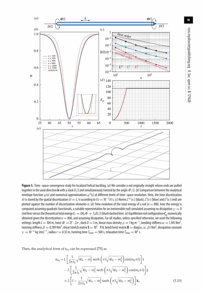
Figure 3. Time–space convergence study for localized helical buckling. (a) We consider a rod originally straight whose ends are pulledtogether in the axial direction kwith a slack D/2 and simultaneously twisted by the angleΦ/2. (b) Comparison between the analyticalenvelope function ϕ(s) and numerical approximations ϕn(s) at different levels of time–space resolution. Here, the time discretizationδt is slaved by the spatial discretization δl = L/n according to δt = 10−3δl s. (c) Norms L∞(ε) (black), L1(ε) (blue) and L2(ε) (red) areplotted against the number of discretization elements n. (d) Time evolution of the total energy of a rod (n= 800, here the energy iscomputed assuming quadratic functionals, a suitable representation for an inextensible rod) simulated assuming no dissipation γ = 0(red line) versus the theoretical total energy EF = (MhΦ + ThD)/2 (black dashed line). (e) Equilibrium rod configuration rneq numericallyobtained given the discretization n= 800, and assuming dissipation. For all studies, unless specified otherwise, we used the followingsettings: length L= 100 m, twistΦ = 27 · 2π , slack D= 3 m, linear mass densityρ = 1 kg m−1, bending stiffnessα = 1.345 Nm2,twisting stiffnessβ = 0.789 Nm2, shear/stretchmatrix S= 105 · 111 N, bend/twist matrixB= diag(α,α,β) Nm2, dissipation constantγ = 10−2 kg (ms)−1, radius r = 0.35 m, twisting time Ttwist = 500 s, relaxation time Trelax = 104 s.

Then, the analytical form of req can be expressed [75] as

req = L[

12π th

√4th − m2

h sech(π s√

4th − m2h

)sin(mhπ s)

]i

− L[

12π th

√4th − m2

h sech(π s√

4th − m2h

)cos(mhπ s)

]j

+ L[

s − 12π th

√4th − m2

h tanh(π s√

4th − m2h

)]k, (3.10)

11


................................................where s = s/L − 0.5 is the normalized arc-length −0.5 ≤ s ≤ 0.5. Here, we make use of equation (3.10) toinvestigate the convergence properties of our solver in the limit of refinement. To compare analytical andnumerical solutions, a metric invariant to rotations about k is necessary. Following Bergou et al. [14], werely on the definition of the envelope ϕ

ϕ = cos θ − cos θmax

1 − cos θmax, θ = arccos(t · k) (3.11)

where θ is the angular deviation of the tangent t from the axial direction k, and θmax is the correspondingmaximum value along the filament. The envelope ϕ relative to the analytical solution of equation (3.10),and ϕn relative to a numerical model of n discretization elements can be estimated via finite differences.This allows us to determine the convergence order of the solver by means of the norms L1(ε), L2(ε) andL∞(ε) of the error ε = ‖ϕ − ϕn‖.

We simulate the problem illustrated in figure 3 at different space–time resolutions. The straight rodoriginally at rest is twisted and compressed at a constant rate during the period Ttwist. Subsequently,the ends of the rod are held in their final configurations for the period Trelax to allow the internalenergy to dissipate (according to the model of §4.1) until the steady state is reached. Simulations arecarried out progressively refining the spatial discretization δl = L/n by varying n = 100–3200 and thetime discretization δt is kept proportional to δl, as reported in figure 3.

As can be seen in figure 3b,c,e the numerical solutions converge to the analytical one with second orderin time and space, consistent with our spatial and temporal discretization schemes. Moreover, to validatethe energy-conserving properties of the solver in the limit of e → 1, we turn off the internal dissipation(figure 3d) and observe that the total energy of the filament EF is constant after Ttwist and matches itstheoretical value EF = (MhΦ + ThD)/2.

3.4.2. Vertical oscillations under gravity

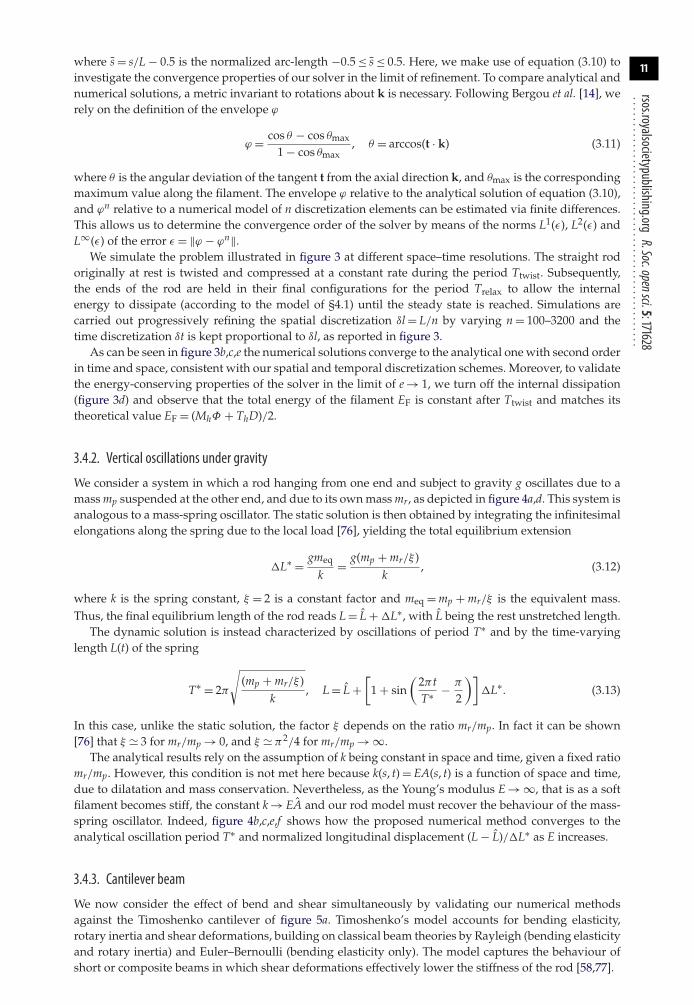
We consider a system in which a rod hanging from one end and subject to gravity g oscillates due to amass mp suspended at the other end, and due to its own mass mr, as depicted in figure 4a,d. This system isanalogous to a mass-spring oscillator. The static solution is then obtained by integrating the infinitesimalelongations along the spring due to the local load [76], yielding the total equilibrium extension

�L∗ = gmeq

k= g(mp + mr/ξ )

k, (3.12)

where k is the spring constant, ξ = 2 is a constant factor and meq = mp + mr/ξ is the equivalent mass.Thus, the final equilibrium length of the rod reads L = L +�L∗, with L being the rest unstretched length.

The dynamic solution is instead characterized by oscillations of period T∗ and by the time-varyinglength L(t) of the spring

T∗ = 2π

√(mp + mr/ξ )

k, L = L +

[1 + sin

(2π tT∗ − π

2

)]�L∗. (3.13)

In this case, unlike the static solution, the factor ξ depends on the ratio mr/mp. In fact it can be shown[76] that ξ � 3 for mr/mp → 0, and ξ � π2/4 for mr/mp → ∞.

The analytical results rely on the assumption of k being constant in space and time, given a fixed ratiomr/mp. However, this condition is not met here because k(s, t) = EA(s, t) is a function of space and time,due to dilatation and mass conservation. Nevertheless, as the Young’s modulus E → ∞, that is as a softfilament becomes stiff, the constant k → EA and our rod model must recover the behaviour of the mass-spring oscillator. Indeed, figure 4b,c,e,f shows how the proposed numerical method converges to theanalytical oscillation period T∗ and normalized longitudinal displacement (L − L)/�L∗ as E increases.

3.4.3. Cantilever beam

We now consider the effect of bend and shear simultaneously by validating our numerical methodsagainst the Timoshenko cantilever of figure 5a. Timoshenko’s model accounts for bending elasticity,rotary inertia and shear deformations, building on classical beam theories by Rayleigh (bending elasticityand rotary inertia) and Euler–Bernoulli (bending elasticity only). The model captures the behaviour ofshort or composite beams in which shear deformations effectively lower the stiffness of the rod [58,77].

12


................................................

2.5

3.5 10

1

10–1

10–2

10–3

10–4

10–5

107 108 109

E1010

1

10–1

10–2

10–3

104 105 106

E107

3.0

2.5

2.0

E1.5

1.0

0.5

00 0.2 0.4 0.6 0.8 1.0

2.0

mr

mr

mp

1.5

1.0

0.5

(L –

L )/

DL*

(L –

L )/

DL*

00 0.2 0.4 0.6

t/T*

t/T*

0.8 1.0

L• L1 L2

E

L• L1 L2

first order

(b)(a) (c)

(e)(d)(f)

|| '||

|| '||

first order

Figure 4. Vertical oscillation under gravity. (a,d) We consider a vertical rod of massmr clamped at the top and with a massmp attachedto the free end. Assuming that the rod is stiff enough (i.e. k � AE = const), it oscillates due to gravity around the equilibrium positionL +�L∗, where�L∗ = g(mp + mr/2)/k with a period T∗ = 2π

√(mp + mr/ξ )/k with ξ � 3 for mp � mr , and ξ � π 2/4

formp mr . Therefore, the rod oscillates according to L(t)= L + [1 + sin(2π t/T∗ − π/2)]�L∗. (a–b) Casemp � mr withmp =100 kg and mr = 1 kg. (b) By increasing the stiffness E = 107, 2 × 107, 3 × 107, 5 × 107, 108, 1010 Pa, the simulated oscillations (redlines) approach the analytical solution (dashed black line). (c) Convergence to the analytical solution in the norms L∞(ε) (black),L1(ε) (blue) and L2(ε) (red) with ε = ‖L(t) − LE (t)‖, where LE is the length numerically obtained as a function of E. (c–d) Casemp mr withmp = 0 kg andmr = 1 kg. (e) By increasing the stiffness E = 104, 2 × 104, 3 × 104, 5 × 104, 105, 2 × 105, 109 Pa, thesimulated oscillations approach the analytical solution. (f ) Convergence to the analytical solution in the norms L∞(ε), L1(ε) and L2(ε)as a function of E. For all studies, we used the following settings: gravity g= 9.81 m s−2, rod density ρ = 103 kg m−3, shear modulusG = 2E/3 Pa, shear/stretchmatrix S= diag(4GA/3, 4GA/3, EA) N, bend/twistmatrix B= diag(EI1, EI2, GI3) Nm2, rest length L= 1 m,rest cross-sectional area A= mr/(Lρ) m2, number of discretization elements n= 100, timestep δt = T∗/106, dissipation constantγ = 0.

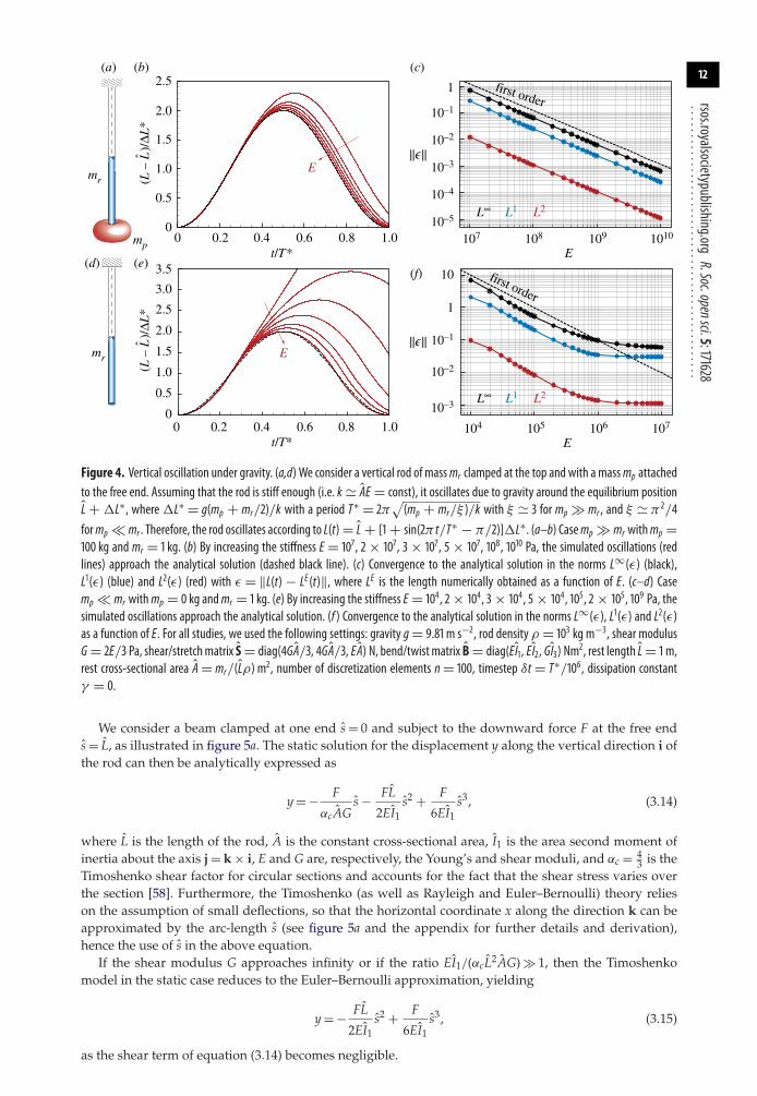
We consider a beam clamped at one end s = 0 and subject to the downward force F at the free ends = L, as illustrated in figure 5a. The static solution for the displacement y along the vertical direction i ofthe rod can then be analytically expressed as

y = − F

αcAGs − FL

2EI1s2 + F

6EI1s3, (3.14)

where L is the length of the rod, A is the constant cross-sectional area, I1 is the area second moment ofinertia about the axis j = k × i, E and G are, respectively, the Young’s and shear moduli, and αc = 4

3 is theTimoshenko shear factor for circular sections and accounts for the fact that the shear stress varies overthe section [58]. Furthermore, the Timoshenko (as well as Rayleigh and Euler–Bernoulli) theory relieson the assumption of small deflections, so that the horizontal coordinate x along the direction k can beapproximated by the arc-length s (see figure 5a and the appendix for further details and derivation),hence the use of s in the above equation.

If the shear modulus G approaches infinity or if the ratio EI1/(αcL2AG) � 1, then the Timoshenkomodel in the static case reduces to the Euler–Bernoulli approximation, yielding

y = − FL

2EI1s2 + F

6EI1s3, (3.15)

as the shear term of equation (3.14) becomes negligible.

13


................................................

i

first order

Timoshenkosecond order

Euler–Bernoulli

F

10–2

k

10–3

10–4

10–5

10–610 102

n

0

–0.01

–0.02

–0.03

–0.04

–0.05

–0.06

–0.070 0.5 1.0 1.5 2.0 2.5 3.0

S

y

(b)

(a)

(c)

|| '||

Figure 5. Time–space convergence study for a cantilever beam. (a) We consider the static solution of a beam clamped at one end s= 0and subject to the downward force F at the free end s= L. (b) Comparison between the Timoshenko analytical y (black lines) andnumerical yn (withn= 400, reddashed lines) vertical displacementswith respect to the initial rod configuration. As a referencewe reportin blue the corresponding Euler–Bernoulli solution. (c) Norms L∞(ε) (black), L1(ε) (blue) and L2(ε) (red) of the error ε = ‖y − yn‖ atdifferent levels of time–space resolution are plotted against the number of discretization elements n. Here, the time discretization δt isslaved by the spatial discretization n according to δt = 10−2δl seconds. For all studies, we used the following settings: rod densityρ =5000 kg m−3, Young’smodulus E = 106 Pa, shearmodulusG = 104 Pa, shear/stretchmatrix S= diag(4GA/3, 4GA/3, EA) N, bend/twistmatrix B= diag(EI1, EI2, GI3) Nm2, downward force F = 15 N, rest length L= 3 m, rest radius r = 0.25 m, dissipation constant γ =10−1 kg (ms)−1, simulation time Tsim = 5000 s.

We compare our numerical model with these results by carrying out simulations of the cantileverbeam of figure 5a in the time–space limit of refinement. As can be noticed in figure 5b the discrete solutionrecovers the Timoshenko one. Therefore, the solver correctly captures the role of shear that reduces theeffective stiffness relative to the Euler–Bernoulli solution. Moreover, our approach is shown to convergeto the analytical solution in all the norms L∞(ε), L1(ε), L2(ε) of the error ε = ‖y − yn‖, where yn is thevertical displacement numerically obtained in the refinement limit.

We note that the norms L∞(ε) and L1(ε) exhibit first-order convergence, while L2(ε) decays with aslope between first and second order. We attribute these results to the fact that while the Timoshenkosolution does not consider axial extension or tension, it does rely on the assumption of small deflections(s = x), therefore effectively producing a dilatation of the rod. On the contrary, our solver does not assumesmall deflections and does not neglect axial extension, because the third entry of the matrix B has thefinite value EA (see figure 5 for details). This discrepancy is here empirically observed to decrease theconvergence order.

These studies, together with the ones reported in the appendix, complete the validation of ournumerical implementation and demonstrate the accuracy of our solver in simulating soft filaments insimple settings.

4. Including interactions and activity: solid and liquid friction, contact andmuscular effects

Motivated by advancements in the field of soft robotics [41,44,45], we wish to develop a robustand accurate framework for the characterization and computational design of soft slender structuresinteracting with complex environments. To this end, we expand the range of applications of ourformalism by including additional physical effects, from viscous hydrodynamic forces in the slender-body limit and surface solid friction to self-contact and active muscular activity. As a general strategy, allnew external physical interactions are accounted for by lumping their contributions into the externalforces and couples F and CL on the right-hand side of the linear and angular momentum balanceequations (2.14) and (2.15). On the other hand, all new internal physical and biophysical effects are

14


................................................

S0 = S1 S2 S3 S4 S5 S6S7

=

b2

b0

b1

b4b3b5 b6

b7

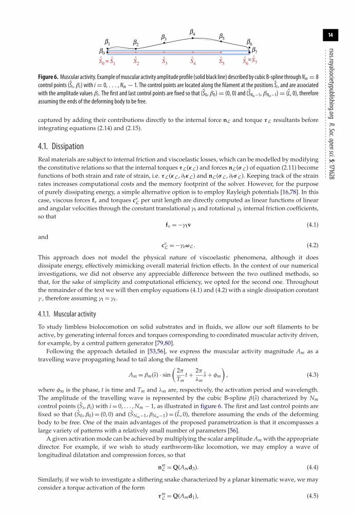
Figure6. Muscular activity. Example ofmuscular activity amplitude profile (solid black line) described by cubic B-spline throughNm = 8control points (Si ,βi) with i = 0, . . . , Nm − 1. The control points are located along the filament at the positions Si , and are associatedwith the amplitude valuesβi . The first and last control points are fixed so that (S0,β0)= (0, 0) and (SNm−1,βNm−1)= (L, 0), thereforeassuming the ends of the deforming body to be free.

captured by adding their contributions directly to the internal force nL and torque τL resultants beforeintegrating equations (2.14) and (2.15).

4.1. DissipationReal materials are subject to internal friction and viscoelastic losses, which can be modelled by modifyingthe constitutive relations so that the internal torques τL(κL) and forces nL(σL) of equation (2.11) becomefunctions of both strain and rate of strain, i.e. τL(κL, ∂tκL) and nL(σL, ∂tσL). Keeping track of the strainrates increases computational costs and the memory footprint of the solver. However, for the purposeof purely dissipating energy, a simple alternative option is to employ Rayleigh potentials [16,78]. In thiscase, viscous forces fv and torques cvL per unit length are directly computed as linear functions of linearand angular velocities through the constant translational γt and rotational γr internal friction coefficients,so that

fv = −γtv (4.1)

andcvL = −γrωL. (4.2)

This approach does not model the physical nature of viscoelastic phenomena, although it doesdissipate energy, effectively mimicking overall material friction effects. In the context of our numericalinvestigations, we did not observe any appreciable difference between the two outlined methods, sothat, for the sake of simplicity and computational efficiency, we opted for the second one. Throughoutthe remainder of the text we will then employ equations (4.1) and (4.2) with a single dissipation constantγ , therefore assuming γt = γr.

4.1.1. Muscular activity

To study limbless biolocomotion on solid substrates and in fluids, we allow our soft filaments to beactive, by generating internal forces and torques corresponding to coordinated muscular activity driven,for example, by a central pattern generator [79,80].

Following the approach detailed in [53,56], we express the muscular activity magnitude Am as atravelling wave propagating head to tail along the filament

Am = βm(s) · sin(

2πTm

t + 2πλm

s + φm

), (4.3)

where φm is the phase, t is time and Tm and λm are, respectively, the activation period and wavelength.The amplitude of the travelling wave is represented by the cubic B-spline β(s) characterized by Nm

control points (Si,βi) with i = 0, . . . , Nm − 1, as illustrated in figure 6. The first and last control points arefixed so that (S0,β0) = (0, 0) and (SNm−1,βNm−1) = (L, 0), therefore assuming the ends of the deformingbody to be free. One of the main advantages of the proposed parametrization is that it encompasses alarge variety of patterns with a relatively small number of parameters [56].

A given activation mode can be achieved by multiplying the scalar amplitude Am with the appropriatedirector. For example, if we wish to study earthworm-like locomotion, we may employ a wave oflongitudinal dilatation and compression forces, so that

nmL = Q(Amd3). (4.4)

Similarly, if we wish to investigate a slithering snake characterized by a planar kinematic wave, we mayconsider a torque activation of the form

τmL = Q(Amd1), (4.5)

15


................................................assuming d2 and d3 to be coplanar to the ground. These two contributions are directly added to theinternal force nL and torque τL resultants.

In the most general case, all deformation modes can be excited by enabling force and torque muscularactivity along all directors d1, d2 and d3, providing great flexibility in terms of possible gaits.

4.1.2. Self-contact

To prevent the filament from passing through itself, we need to account for self-contact. As a generalstrategy, we avoid enforcing the presence of boundaries via Lagrangian constraints as their formulationmay be cumbersome [81], impairing the modularity of the numerical solver. We instead resort tocalculating forces and torques directly and replacing hard constraints with ‘soft’ displacement–forcerelations.

Our self-contact model introduces additional forces Fsc acting between the discrete elements incontact. To determine whether any two cylindrical elements are in contact, we calculate the minimum

distance dijmin between edges i, j by parametrizing their centre lines ci(h) = si + h(si+1 − si) so that

dijmin = max

h1,h2∈[0,1]‖ci(h1) − cj(h2)‖. (4.6)

If dijmin is smaller than the sum of the radii of the two cylinders, then they are considered to be in contact

and penalty forces are applied to each element as a function of the scalar overlap εij = (ri + rj − dijmin),

where ri and rj are the radii of edges i and j, respectively. If εij is smaller than zero, then the two edges

are not in contact and no penalty is applied. Denoting as dijmin the unit vector pointing from the closest

point on edge i to the closest point on edge j, the self-contact repulsion force is given by

Fsc = H(εij) · [−kscεij − γsc(vi − vj) · dijmin]dij

min, (4.7)

where H(εij) denotes the Heaviside function and ensures that a repulsion force is produced only incase of contact (εij ≥ 0). The first term within the square brackets expresses the linear response to theinterpenetration distance as modulated by the stiffness ksc, while the second damping term modelscontact dissipation and is proportional to the coefficient γsc and the interpenetration velocity vi − vj.

4.1.3. Contact with solid boundaries

To investigate scenarios in which filaments interact with the surrounding environment, we must alsoaccount for solid boundaries. By implementing the same approach outlined in the previous section,obstacles and surfaces are modelled as soft boundaries allowing for interpenetration with the elementsof the rod (figure 7). The wall response Fw

⊥ balances the sum of all forces F⊥ that push the rod against thewall, and is complemented by the other two components which help prevent possible interpenetrationdue to numerics. The interpenetration distance ε triggers a normal elastic response proportional to thestiffness of the wall, while a dissipative term related to the normal velocity component of the filamentwith respect to the substrate accounts for a damping force, so that the overall wall response reads

Fw⊥ = H(ε) · (−F⊥ + kwε − γwv · uw

⊥)uw⊥ , (4.8)

where H(ε) denotes the Heaviside function and ensures that a wall force is produced only in case ofcontact (ε ≥ 0). Here, uw

⊥ is the boundary outward normal (evaluated at the contact point, that is thecontact location for which the normal passes through the centre of mass of the element), and kw and γw

are, respectively, the wall stiffness and dissipation coefficients.

4.1.4. Isotropic and anisotropic surface friction

Solid boundaries also affect the dynamics of the filament through surface friction, a complex physicalphenomenon in which a range of factors are involved, from roughness and plasticity of the surfaces incontact to the kinematic initial conditions and geometric set-up. Here, we adopt the Amonton–Coulombmodel, the simplest of friction models.

This model relates the normal force pushing a body onto a substrate to the friction force through thekinetic μk and static μs friction coefficients, depending on whether the contact surfaces are in relativemotion or not.

Despite the simplicity of the model, its formulation and implementation may not necessarily bestraightforward, especially in the case of rolling motions. Given the cylindrical geometry of our filaments,

16


................................................

F^

Fw^

v

r

d uw^

'

Figure 7. Contact model with solid boundaries. Obstacles and surfaces (grey) are modelled as soft boundaries allowing for theinterpenetration ε = r − d with the elements of the filament (blue) characterized by radius r and distance d from the substrate. Thesurface normal uw⊥ determines the direction of the wall’s response Fw⊥ to contact. We note that Fw⊥ balances the sum of all forces F⊥ thatpush the rod against the wall, and is complemented by the other two components, which allow it to amend to possible interpenetrationdue to numerics. These components are an elastic one (kwε) and a dissipative one (γwv · uw⊥), where kw and γw are, respectively, thewall stiffness and dissipation coefficients.

uw^

uw¥

uw^

uw^

v¥uw

||

F||

F||

r

r

w¥

w¥

v||

v||

F^

F^

Froll

Froll

vcont

vcont

vslip

T¥

T¥

v||

v

(b)(a)

(c)

Figure 8. Surface friction. (a) The forces produced by friction effects between an element of the rod and the substrate are naturallydecomposed into a lateral component in the direction uw‖ = t × uw⊥ and a longitudinal one in the direction uw× = uw⊥ × uw‖ . We notethat in generaluw× �= t. The notation x⊥, x‖, x× denotes the projection of the vector x in the directionsuw⊥,u

w‖ ,u

w×. (b,c) Kinematic and

dynamic quantities at play at any cross section in the case of (b) rolling and slipping and (c) pure rolling motion. Red arrows correspondto forces and torques, green arrows correspond to velocities, and black arrows correspond to geometric quantities.

the effect of surface friction can be decomposed into a longitudinal component associated with purelytranslational displacements, and a lateral component associated with both translational and rotationalmotions (figure 8). We use the notation x⊥, x‖, x× to denote the projection of the vector x in the directionsuw

⊥ , uw‖ , uw× , as illustrated in figure 8.

The longitudinal friction force Flong is opposite to either the resultant of all forces F× acting on anelement (static case) or to the translational velocity v× (kinetic case) along the direction uw× (figure 8).The Amonton–Coulomb model then reads

Flong =

⎧⎪⎪⎨⎪⎪⎩

− max(|F×|,μs|F⊥|) · F×|F×| if |v×| ≤ vε,

−μk|F⊥| · v×|v×| if |v×|> vε,

17


................................................where vε → 0 is the absolute velocity threshold value employed to distinguish between static (|v×| ≤ vε)and kinetic (|v×|> vε) cases. We define vε in a limit form to accommodate the fact that inequalities arenumerically evaluated up to a small threshold value. The static friction force is always equal and oppositeto F× up to a maximum value proportional to the normal force |F⊥| through the coefficient μs. Thekinetic friction force is instead opposite to the translational velocity v×, but does not depend on its actualmagnitude and is proportional to |F⊥| via μk. In general μs >μk, so that it is harder to set a body intomotion from rest than to drag it.

The lateral displacement of a filament in the direction uw‖ = uw× × uw

⊥ is associated with bothtranslational (v‖) and rotational (ω× =ω×uw×) motions, as illustrated in figure 8b,c. In this case, thedistinction between static and kinetic friction does not depend on v‖, but on the relative velocity (alsoreferred to as slip velocity) between the rod and the substrate

vslip = v‖ + vcont, vcont = ruw⊥ × ω×, (4.9)

where vcont is the local velocity of the filament at the contact point with the substrate, due to the axialcomponent of the angular velocity ω×.

In the static or no-slip scenario (vslip = 0), the linear momentum balance in the direction uw‖ , and

the angular momentum balance about the axis uw× express a kinematic constraint between the linearacceleration auw

‖ and angular acceleration ω× = (uw⊥ × auw

‖ )/r, so that

(F‖ + Froll)uw‖ = dm · auw

‖ (4.10)

and

T×uw× − ruw

⊥ × Frolluw‖ = J ·

uw⊥ × auw

‖r

, (4.11)

where F‖ = F‖uw‖ and T× = T×uw× are the forces and torques acting on the local element, and Froll =

Frolluw‖ is the rolling friction force at the substrate–filament interface necessary to meet the no-slip

condition. By recalling that a disk mass second moment of inertia about uw× is J = r2 dm/2, the abovesystem can be solved for the unknown a and Froll, yielding

Froll = − rF‖ − 2T×3r

uw‖ . (4.12)

Therefore, the lateral friction force Flat and the associated torque ClatL can be finally expressed as

Flat =

⎧⎪⎪⎪⎨⎪⎪⎪⎩

max(|Froll|,μrs|F⊥|) · Froll

|Froll|if |vslip| ≤ vε

−μrk|F⊥| · vslip

|vslip| if |vslip|> vε, Clat

L = Q(Flat × ruw⊥),

where μrs and μr

k are, respectively, the rolling static and kinetic friction coefficients.So far we have considered isotropic friction by assuming that the coefficients μs and μk are constant

and independent of the direction of the total acting forces (static case) or relative velocities (kinetic case).Nevertheless, frictional forces may be highly anisotropic. For example, the anisotropy caused by thepresence of scales on the body of a snake crucially affects gaits and performance [82,83].

The Amonton–Coulomb model can be readily extended to account for anisotropic effects by simplyassuming the friction coefficients μs and μk to be functions of a given reference direction. The natureof these functions depends on the specific physical problems under investigation. An example of thisapproach is illustrated in §5.2 in the context of limbless locomotion. Isotropic and anisotropic frictionvalidation benchmarks are presented in the appendix.

4.1.5. Hydrodynamics

We also extend our computational framework to address flow–structure interaction problems. Inparticular, we consider the case in which viscous forces dominate over inertial effects, i.e. we considersystems in which the Reynolds number Re = ρf UL/μ 1 where ρf and μ are the density and dynamicviscosity of the fluid, respectively, and U is the characteristic velocity of the rod. Under these conditions,the drag forces exerted by the fluid on our filaments can be determined analytically within the contextof slender-body theory [84,85] (for more advanced and accurate viscous flow models we refer the reader

18


................................................to [31–36]). At leading order resistive force line densities scale linearly with the local rod velocities vaccording to

fH = − 4πμln(L/r)

(I − 1

2tTt)

v. (4.13)

We note that the matrix (I − 12 tTt) introduces an anisotropic effect for which

fH‖ = − 2πμ

ln(L/r)|(v · t)t|, fH

⊥ = − 4πμln(L/r)

|v − (v · t)t|, (4.14)

where fH‖ = (fH · t)t and fH

⊥ = fH − fH‖ are, respectively, tangential and orthogonal viscous drag

components. The coupling of liquid environment, filament mechanics and muscular activity provides aflexible platform to characterize biological locomotion at the microscopic scale (bacteria, protozoa, algae,etc.) and to design propulsion strategies in the context of artificial micro-swimmers [45,86].

5. ApplicationsWe now proceed to illustrate the capabilities of our solver with three different applications. We considerfirst a static problem in which self-contact, bending and twist give rise to the classic out-of-planeconfigurations denoted as plectonemes [40], while the addition of stretching and shearing produces adifferent type of experimentally observed solutions, known as solenoids [40]. Then we turn our attentionto two dynamic biophysical problems in which an active filament interacts with a solid and a liquidenvironment, exhibiting qualitatively different optimal biolocomotion strategies. We emphasize here thatone of the main points of these biolocomotion studies, besides verifying the versatility and predictioncapabilities of our solver in biophysical settings, is to demonstrate its practical use in an inverse(optimization) design process, which typically represents a demanding stress test for any simulationalgorithm, as unusual parameter sets or conditions are explored.

5.1. Plectonemes and solenoidsWhen an inextensible rod is clamped at one end and twisted a sufficiently large number of times at theother end, it becomes unstable, coils up and generates a characteristic structure known as a plectoneme[87]. While this behaviour has been well characterized both theoretically and experimentally [87], itsanalogue for highly extensible filaments has been largely ignored [40]. In particular, for large extensionaland twisting strains qualitatively different solutions arise, such as those corresponding to tightly packedsolenoidal structures [40] whose properties are as yet poorly understood, and whose importance hasonly recently been recognized in the context of soft robotics and artificial muscles [41–44].

Given the broad scope of our computational framework, we can now study the formation of bothsolenoids and plectonemes. As illustrated in figure 9a, a soft rod of Young’s modulus E = 106 Pa isclamped at one end, and subject to an axial load F, while also being twisted R times at the otherend. As experimentally and theoretically observed for F = 0, i.e. in the absence of stretching (L/L ≈ 1),plectonemes are generated (figure 9b). When the load F is increased so that the elongation of the rodapproaches L/L ≈ 1.15, solenoids arise as predicted in [40] and illustrated in figure 9c. This test case,therefore, shows the ability of our solver to qualitatively capture different instability mechanisms, drivenby the competition between the different modes of deformation of the rod. We leave the details ofthe explanation of the phase diagram for the formation of plectonemes, solenoids and intermediatestructures [40] for a later study.

5.2. SlitheringThe mechanics of slithering locomotion typical of snakes has been extensively investigatedexperimentally [83,88,89], theoretically [82,90,91] and computationally [92,93]. While biologicalexperiments have provided quantitative insights, theoretical and computational models have beeninstrumental to characterize qualitatively the working principles underlying snake locomotion.Although these models implement different levels of realism, they generally rely on a number ofkey simplifications. Typically, theoretical models assume planar deformations [82] and/or disregardmechanics by prescribing body kinematics [91]. Computational models offer a more realisticrepresentation, but they have mostly been developed for and tailored to robotic applications [92,93].For example, snakes are often modelled as a relatively small set of hinges and/or springs representingpointwise localized actuators that connect contiguous rigid segments. Therefore, they do not account

19


................................................(a)

(c)

(b)

RF

Figure 9. Formation of plectonemes and solenoids. (a) We consider a soft rod clamped at one end, subject to a constant verticalload F and twisted R times at the other end. (b) Formation of a plectoneme for F = 0 (leading to the total elongation L/L≈ 1)and R= 4. (c) Formation of a solenoid for F = 300 N (leading to the total elongation L/L≈ 1.15) and R= 13. Settings: lengthL= 1 m, radius r = 0.025 m, mass m= 1 kg, Young’s modulus E = 106 Pa, shear modulus G = 2E/3 Pa, shear/stretch matrix S=diag(4GA/3, 4GA/3, EA) N, bend/twist matrix B= diag(EI1, EI2, GI3) Nm2, dissipation constant γ = 2 kg (ms)−1, ksc = 104 kg s−2,γsc = 10 kg s−1, discretization elements n= 100, timestep δt = 0.01δl s, Ttwist = 75 s, Trelax = 50 s.

for the continuum nature of elastic body mechanics and biological muscular activity. Moreover, in robotreplicas the critical feature of friction anisotropy is commonly achieved through the use of wheels [89].As a consequence computational models often assume only two sources of anisotropy, in the tangentialand lateral direction with respect to the body. This is in contrast with biological experiments [83] thathighlight the importance of all three sources of anisotropy, namely forward, backward and lateral.

Our approach complements those previous attempts by accounting for physical and biological effectswithin a continuum framework (equations (2.12)–(2.15)). In this section, we demonstrate the qualitativeand quantitative capabilities of our solver by reverse engineering optimal slithering gaits that maximizeforward speed.

We consider a soft filament of unit length actuated via a planar travelling torque wave of muscularactivity in the direction perpendicular to the ground. The interaction with the substrate is characterized

by the ratios μfk :μb

k :μrk = 1 : 1.5 : 2 and μf

s :μbs :μr

s = 1 : 1.5 : 2 with μfs = 2μf

k, as experimentally observedfor juvenile Pueblan milk snakes on a moderately rough surface [83]. The value of the friction coefficient

μfk is set so that the ratio between inertial and friction forces captured by the Froude number is Fr =

(L/T2m)/(μf

kg) = 0.1, as measured for these snakes [83].In the spirit of [53,56,57], we wish to identify the fastest gaits by optimizing the filament muscular

activity. The torque wave generated by the snake is parametrized according to §4.1.1 and is characterizedby Nm = 6 control points and a unit oscillation period Tm, so that overall we optimize for five parameters,four of which are responsible for the torque profile along the rod (β1, β2, β3, β4), while the last onerepresents the wavenumber 2π/λm (see §4.1.1).

These parameters are left free to evolve from an initial zero value, guided by an automatedoptimization procedure that identifies the optimal values that maximize the snake’s forward averagespeed vfwd

max over one activation cycle Tm. The algorithm of choice is the Covariance Matrix Adaptation-Evolution Strategy [94,95] (CMA-ES) which has proved effective in a range of biophysical andengineering problems, from the optimization of swimming gaits [53], morphologies [56,57] and collectivedynamics [55] to the identification of aircraft alleviation schemes [96] or virus traffic mechanisms [52].The CMA-ES is a stochastic optimization algorithm that samples generations of p parameter vectorsfrom a multivariate Gaussian distribution N . Here each parameter vector represents a muscularactivation instance, and every generation entails the evaluation of p = 60 different gaits. The covariancematrix of the distribution N is then adapted based on successful past gaits, chosen according to theircorresponding cost function value f = vfwd

max, until convergence to the optimum.The course of the optimization is reported in figure 10 together with the kinematic details of the

identified fastest gait. As can be noticed in figure 10e,f the forward scaled average speed approaches

20


................................................

0.6

0.50.6

0.4

0.2

velo

city

0

–0.20 2 4 6 8 10

head tail

0.2L

0.4

0.3f

0.2

0.1

0 10 20generations t/Tm

30 40

(a) (c) (d)(b)

(e) ( f ) (g)

Figure 10. Optimal lateral undulation gait. (a–d) Instances at different times of a snake characterized by the identified optimal gait.(e) Evolution of the fitness function f = vfwdmax as a function of the number of generations produced by CMA-ES. Solid blue, solidred and dashed black lines represent, respectively, the evolution of f corresponding to the best solution, the best solution withinthe current generation, and the mean generation value. (f ) Scaled forward (red) and lateral (blue) centre of mass velocities versusnormalized time. (g) Gait envelope over one oscillation period Tm. Red lines represent head and tail displacement in time. Settings: Froudenumber Fr = 0.1, length L= 1 m, radius r = 0.025 m, densityρ = 103 kg m−3, Tm = 1 s, Young’s modulus E = 107 Pa, shear modulusG = 2E/3 Pa, shear/stretch matrix S= diag(4GA/3, 4GA/3, EA) N, bend/twist matrix B= diag(EI1, EI2, GI3) Nm2, dissipation constantγ = 5 kg (ms)−1, gravityg= 9.81 m s−2, friction coefficient ratiosμf

k :μbk :μ

rk = 1 : 1.5 : 2 andμf

s :μbs :μ

rs = 1 : 1.5 : 2withμf

s =2μf

k, friction threshold velocity vε = 10−8 m s−1, ground stiffness and viscous dissipation kw = 1 kg s−2 and γw = 10−6 kg s−1,discretization elementsn= 50, timestepδt = 2.5 · 10−5 Tm, wavelengthλm = 0.97L, phase shiftφm = 0, torqueB-spline coefficientsβi=0,...,5 = {0, 17.4, 48.5, 5.4, 14.7, 0} Nm, bounds maximum attainable torque |β|maxi=0,...,5 = 50 Nm.

vfwdmax � 0.6, consistent with experimental evidence [97]. Moreover, CMA-ES finds that the optimal

wavelength is λm � L (figure 10g), again consistent with biological observations [83,98]. Thus, this valueof wavelength strikes a balance between thrust production and drag minimization within the mechanicalconstraints of the system.

We note that a rigorous characterization of slithering locomotion would require the knowledge of anumber of biologically relevant parameters (Young’s and shear moduli of muscular tissue, maximumattainable torques, etc.) and environmental conditions (terrain asperities, presence of pegs, etc.) and goesbeyond the scope of the present work. Nevertheless, this study illustrates the robustness, quantitativeaccuracy and suitability of our solver for the characterization of biolocomotion phenomena.

5.2.1. Swimming

We finally turn to apply the inverse design approach outlined in the previous section to the problemof swimming at low Reynolds numbers where viscous forces dominate inertial effects. We maintain theexact same set-up as in the slithering case, while we change the environment from a solid substrate toa viscous fluid. The flow-filament interaction is then modelled via slender-body theory, as illustrated in§4.1.5.

Once again we inverse design planar optimal gaits for forward average speed f = vfwdmax within one

activation cycle Tm, by employing the same muscular activity parametrization as for slithering. To verifya posteriori the biological relevance of the identified optimal solution, we consider the case of the seaurchin spermatozoon Echinus esculentus [99], which swims by means of helical or planar waves travellingalong its flagella of length Ls � 40 µm. The gait corresponding to planar swimming is characterized bykinematic undulations of wavelength λs < Ls and frequency fs � 2.8. At Re � 10−4 the spermatozoonattains the scaled velocity vs = Us/(fsLs) � 0.08 ± 0.03, where Us is the dimensional cruise speed [99].Although this gait may not be the absolute optimal planar locomotion pattern, the fact that it is replicatedin a large number of organisms [85] suggests that it captures some effective features that we expect toqualitatively recover via our numerical optimization.

21


................................................

0.06

0.05

0.04

0.03f

0.02

0.01

0

0.060.050.040.030.02ve

loci

ty0.01

0–0.01

10 20 30generations

40 50 60 0 2 4t/Tm

6 8 10

head tail

0.2L

(a) (c) (d)(b)

(e) ( f ) (g)

Figure 11. Optimal planar swimming gait at low Reynolds number. (a–d) Instances at different times of a filament swimming accordingto the identified optimal gait. (e) Evolution of the fitness function f = vfwdmax as a function of the number of generations produced byCMA-ES. Solid blue, solid red and dashed black lines represent, respectively, the evolution of f corresponding to the best solution, thebest solution within the current generation, and the mean generation value. (f ) Scaled forward (red) and lateral (blue) centre of massvelocities versus normalized time. (g) Gait envelope over one oscillation period Tm. Red lines represent head and tail displacementin time. Settings: Reynolds number Re= 10−4, length L= 1 m, radius r = 0.025 m, filament density ρ = 103 kg m−3, Tm = 1 s,Young’s modulus E = 107 Pa, shear modulus G = 2E/3 Pa, shear/stretch matrix S= diag(4GA/3, 4GA/3, EA) N, bend/twist matrixB= diag(EI1, EI2, GI3) Nm2, dissipation constant γ = 5 kg (ms)−1, discretization elements n= 50, timestep δt = 2.5 × 10−5 Tm,wavelength λm = 2.6L, phase shift φm = 0, torque B-spline coefficients βi=0,...,5 = {0, 50, 50, 50, 50, 0} Nm, bounds maximumattainable torque |β|maxi=0,...,5 = 50 Nm.

The course of the optimization is reported in figure 11 together with the kinematic details of theidentified fastest gait. As can be noted in figure 11e,f, the forward average scaled speed and wavelengthapproach vfwd

max � 0.055 and λm � 0.38L are qualitatively and quantitatively consistent with experimentalevidence [99].

As in the previous section, we note that a rigorous characterization of optimal swimming at lowReynolds numbers would require the knowledge of a number of biologically relevant parameters andenvironmental conditions, a careful comparison with a rich body of literature [33,35,36,85], and goesbeyond the scope of the present work. Nevertheless, this and the previous study illustrate how theinterplay between filament mechanics and the surrounding environment crucially affects propulsivegaits, as is biologically evident and automatically recovered via our numerical inverse design approach.

6. ConclusionsWe have presented a versatile implementation of the Cosserat rod model for the simulation ofsoft filaments deforming in three-dimensional space. These filaments at any given cross section canexperience all deformation modes, namely normal and orthonormal bending, twisting, stretching andshearing. Particular emphasis is placed in realistically accounting for substantial axial extensions andshear strains, targeting emerging soft robotic applications. The solver also handles self-contact, muscularactivity, solid boundaries, isotropic and anisotropic friction as well as hydrodynamics. The outcome is asimple algorithm suitable to tackle a plethora of engineering and biophysical phenomena.

We verified this against a battery of benchmark problems entailing different physical aspectsand boundary conditions, and used it to solve a range of forward and inverse problems spanningmechanics and biophysics. In particular, we studied the formation of solenoids and plectonemes andthe evolutionary optimization of terrestrial limbless locomotion and swimming.

Our results demonstrate the utility of a modelling approach based on Cosserat rods in a wide rangeof settings that involve active and passive soft filaments, broadening the scope of previous studies. We

22


................................................particularly emphasize that our robust computational approach allows us to approach the solution of aninverse problem by coupling our method with evolutionary strategies successfully, without the problemsassociated with the (often unforeseen) variety of candidate solutions produced throughout the process.Ongoing work involves its coupling to realistic high Reynolds number flow solvers [100], its integrationwith sensory feedback models for the characterization of locomotory neural circuitry [80], and its use forthe rational design of biohybrid robots [45,101].

Data accessibility. Our software implementing the study cases presented in the manuscript and in the appendix is publiclyavailable at https://github.com/mattialab/elastica.git.Authors’ contributions. M.G. and L.M. designed the study. M.G. and A.G.M. implemented the software. M.G. and L.H.D.carried out the analysis of the results. M.G., L.H.D. and L.M. wrote the manuscript.Competing interests. The authors declare no competing interests.Funding. We thank the Swiss National Science Foundation and the Blue Waters project (OCI-0725070, ACI-1238993),a joint effort of the University of Illinois at Urbana-Champaign and its National Center for SupercomputingApplications, for partial support (M.G.), and the Harvard MRSEC grant NSF DMR 14-20570, Harvard Biomatter grantNSF DMR 33985 and ARO W911NF-15-1-016 for additional support (L.M.).Acknowledgements. We thank Nicholas Charles for a careful reading of and comments on the paper.

Appendix A. Lagrangian governing equationsThe following shows the conversion of governing equations for unstretchable filaments from thelaboratory to material frame of reference. Note that in the Governing equations and Numerical methodsections of the main text, all terms are scaled appropriately by the local dilatation to account forstretching.

The time and space derivatives of the centreline r(s, t) are associated with the velocity v and tangentfield t

v = ∂r∂t

and t = ∂r∂s

, (A 1)

with |t| = 1, since s is the current arc-length.Similarly, time and space derivatives of the material frame Q, due to the orthonormality of the

directors, are associated by definition with the angular velocity ω and generalized curvature κ vectors,so that

∂dj

∂t= ∂(QT ej)

∂t= ∂QT

∂tej = ∂QT

∂tQdj = ω × dj, j = 1, 2, 3 (A 2)

and∂dj

∂s= ∂(QTej)

∂s= ∂QT

∂tej = ∂QT

∂sQdj = κ × dj, j = 1, 2, 3, (A 3)

where the equivalences ∂tQT · Q = ω × (·) and ∂sQT · Q = κ × (·) hold. These kinematic equationscombined with the linear and angular momentum balance laws at a cross section [102] yield thegoverning equations for the Cosserat rod

∂r∂t

= v, (A 4)

∂dj

∂t= ω × dj, j = 1, 2, 3, (A 5)

∂(ρAv)∂t

= ∂n∂s

+ f (A 6)

and∂h∂t

= ∂τ

∂s+ ∂r∂s

× n + c, (A 7)

where ρ is the constant material density, A is the cross-sectional area in its current state (so that ρAv isthe linear momentum line density), h(s, t) is the angular momentum line density, n(s, t) and τ (s, t) are theinternal force and torque resultants, and f and c are external body force and torque line densities.

The internal force n and torque τ resultants depend on the geometric and material properties of thefilament. This dependence is embedded via the material or constitutive laws, which must be frameinvariant, rendering their definition in a Lagrangian setting most natural. Moreover, we note that theangular momentum line density can be readily expressed in the material frame as Qh = hL = ρIωL,where the tensor I is the second area moment of inertia which, assuming circular cross sections, takes

https://github.com/mattialab/elastica.git

23


................................................the form

I =

⎛⎜⎝I1 0 0

0 I2 00 0 I3

⎞⎟⎠= A2

4π

⎛⎜⎝1 0 0

0 1 00 0 2

⎞⎟⎠= A2

4πdiag(1,1,2).

To derive the Lagrangian form of the angular momentum equation, we begin with the definition ofthe material frame

dj = QTej, j = 1, 2, 3 (A 8)

and definitions of time and space derivatives of its frame directors

∂dj

∂t= ω × dj, j = 1, 2, 3 (A 9)

and∂dj

∂s= κ × dj, j = 1, 2, 3. (A 10)

We can use these definitions to establish relationships between time and space derivatives of thelaboratory and material frames.

∂x∂t

= ∂(QTxL)∂t

(A 11)

=∂(∑3

j=1 djxLj)

∂t(A 12)

=3∑

j=1

∂t(djxLj) (A 13)

=3∑

j=1

(∂tdj)xLj +3∑

j=1

dj(∂txLj) (A 14)

=3∑

j=1

(ω × dj)xLj +3∑

j=1

dj(∂txLj) (A 15)

∂x∂t

= ω × (QTxL) + QT xL∂t

, (A 16)

and∂x∂s

= κ × (QTxL) + QT xL∂s

. (A 17)

Because the second moment of inertia is defined in the material frame, the governing equation for theangular momentum is also most naturally expressed in the material frame (I in the laboratory frame isa function of space and time rendering its use cumbersome, while IL is a constant and, in our isotropiccase, diagonal matrix in the material frame). We can use equations (A 16) and (A 17) to convert all of theterms in equation (A 7) to the material frame.

∂(ρIω)∂t

= QT ∂(ρIω)L∂t

+ ω × (QT(ρIω)L) (LHS) (A 18)

∂τ

∂s= QT ∂τL

∂t+ ω × (QTτL) (RHS) (A 19)

∂r∂s

× n = QT(∂r∂s

)L

× QTnL (RHS) (A 20)

and c = QTcL (RHS). (A 21)

Multiplying by Q and noting that Iω = QTILωL yields our final governing equation for the angularmomentum, expressed in the material frame

∂(ρILωL)∂t

= ∂τL∂s

+ κL × τL + Q∂r∂s

× nL + (ρILωL) × ωL + cL. (A 22)

Aside from the balance of angular momentum, converting equations (A 5) and (A 6) to the material framesimply requires a direct application of the definition of the material frame to the RHS quantities.

24


................................................

linearcurrent

Mooney-RivlinNeo-Hookean

1.21.11.0e

0.90.80.7 1.3

20

0

–20

–40

F(N

)

Figure 12. Comparison with hyperelastic models. Load response in a stretched rubber beam for different models.

Appendix B. Axial stretch comparison with Neo-Hookean andMooney–Rivlin modelsWe consider the simple example of a beam subject to axial stretching and compare the load responsepredicted by our approach (that combines linear stress–strain constitutive laws and cross-sectionalarea rescaling) with Neo-Hookean [60] and Mooney–Rivlin models [61,62] for hyperelastic materials.We assume an initial length L = 100 mm and cross section A = 10 mm2. As the beam is stretched thecross-sectional area decreases. In one-dimensional, the Neo-Hookean model reads:

lime→1

E = 6C10,

α = 2C10

(e − 1

e2

)e

and F = αA = αAe

= 2C10A(

e − 1e2

),

where α is the stress, e = L/L is the elongation factor (related to the strain σ = e − 1), C10 is a materialproperty to be determined experimentally and that in the limit of small strains (e → 1) is related to theYoung’s modulus E, as above indicated. In one-dimensional, the Mooney–Rivlin model reads:

lime→1

E = 6(C10 + C01),

α = 2C10

(e2 − 1

e

)+ 2C01

(e2 − 1

e

)1e

,

and F = αA = αAe

= Ae

[2C10

(e2 − 1

e

)+ 2C01

(e2 − 1

e

)1e

],

where C10 and C01 are material properties to be determined experimentally and that in the limit of smallstrains (e → 1) are related to the Young’s modulus E as indicated above. In our approach the load reads

F = AEσ = AE(e − 1) = Ae

E(e − 1).

Assuming that the beam is made of rubber with E = 107 Pa, and that in the Mooney–Rivlin model C10 =C01, we obtain the load responses illustrated in figure 12. As can be noted our approach reasonablyapproximates more advanced hyperelastic models within a 30% deformation range.

25


................................................Appendix C. Time discretizationTo advance the discrete system of equations (3.6)–(3.9), we choose the energy conserving, second-orderposition Verlet time integration scheme. This allows us to write a full iteration from time t to t + δt as

ri

(t + δt

2

)= ri(t) + δt

2· vi(t), i = [1, n + 1] (C 1)

Qi

(t + δt

2

)= exp

[δt2

ωiL(t)]

· Qi(t), i = [1, n] (C 2)

vi(t + δt) = vi(t) + δt · dvi

dt

(t + δt

2

), i = [1, n + 1] (C 3)

ωiL(t + δt) = ωi

L(t) + δt · dωiL

dt

(t + δt

2

), i = [1, n] (C 4)

ri(t + δt) = ri

(t + δt

2

)+ δt

2· vi

(t + δt

2

)i = [1, n + 1] (C 5)

and Qi(t + δt) = exp[δt2

ωiL

(t + δt

2

)]· Qi

(t + δt

2

). i = [1, n]. (C 6)

The time integrator is structured in three blocks: a first half step position update (equations (C 1) and(C 2)), followed by the evaluation of local accelerations (equations (C 4) and (C 5)), and finally, thesecond half step position update (equations (C 5) and (C 6)). Therefore, the second-order position Verletscheme entails only one right-hand side evaluation of equations (3.8) and (3.9), the most computationallyexpensive operation. We also emphasize that for the numerical integration of equations (C 2) and (C 6)the Rodrigues formula is employed, implying the direct use of ωL instead of ω = QTωL. By foregoingan implicit integration scheme we can quickly incorporate a number of additional physical effects andsoft constraints. This algorithm strikes a balance between computing costs, numerical accuracy andimplementation modularity.

Appendix D. Discrete operatorsThe discrete operators �h : {R3}N → {R3}N+1 and Ah : {R3}N → {R3}N+1 take the form

yj=1,...,N+1 =�h(xi=1,...,N) =

⎧⎪⎪⎨⎪⎪⎩

x1 if j = 1,

xj − xj−1 if 1< j ≤ N

−xN if j = N + 1,

,

yj=1,...,N+1 =Ah(xi=1,...,N) =

⎧⎪⎪⎪⎪⎪⎨⎪⎪⎪⎪⎪⎩

x1

2if j = 1,

xj + xj−1

2if 1< j ≤ N

xN

2if j = N + 1.

,

We note that �h and Ah operate on a set of N vectors and return N + 1 vectors of differences or convertintegrated quantities to point-wise, respectively, consistent with equations (3.8) and (3.9).

Appendix E. Derivation of the vertical displacement of a Timoshenkocantilever beamWe briefly derive here the analytical expression of the vertical displacement y of equation (3.14) for thecantilever beam problem of figure 5a. To do so we make use of the free body diagram of figure 13,and of the constitutive relations of table 1. Moreover, we disregard axial extension and assume smalldeformations so that the coordinate x (along the direction k) is approximated by the arc-length s.

Recalling that the bending strain is the space derivative of the bending angle ψ (figure 13), we maywrite

∂ψ

∂s= M

EI1, (E 1)

where M is the bending moment, E the Young’s modulus, and I1 is the second area moment of inertiaabout the axis j = k × i (figure 5a). The shear angle θ , as illustrated in figure 13, is the difference between

26


................................................y

x

M

V

V + dV

M + dM perpendicular to face

tangent to neutral axis

q

y —dydx

Figure 13. Free body diagramof an infinitesimal beamelement. The sketch represents an infinitesimal element undergoing bending andshear deformations, assuming small deflections so that x � s. The bending moment is denoted as M, the shear force as V, the verticaldisplacement as y. The bending angleψ , the shear angle θ and the slope of the vertical displacement dxy are related to each other sothatψ = θ + dxy.

the bending angle and the slope of the centreline, so that

ψ − ∂y∂s

= VαcAG

, (E 2)

where V is the shear force, A is the cross-sectional area, G is the shear modulus and αc is the Timoshenkofactor [58]. If a point load F is applied downward at s = L, where L is the length of the rod, a free bodydiagram of the beam yields M = −F(L − s) and V = F, so that

∂ψ

∂s= −F(L − s)

EI1(E 3)

and

ψ − ∂y∂s

= FαcAG

. (E 4)

By integrating equation (E 3) with boundary conditions ψ = 0 at s = 0, injecting the solution ψ intoequation (E 4), and integrating again with boundary conditions y = 0 at s = 0, we obtain

y = − F

αcAGs − FL

2EI1s2 + F

6EI1s3. (E 5)

Appendix F. Further validationsF.1. Euler buckling instabilityEuler buckling involves a single straight isotropic, inextensible and unshearable rod subject to an axialload F, as depicted in figure 14a. The critical axial load Fc that the rod can withstand before bending canbe expressed analytically [3] as

Fc = π2EI(bL)2 , (F 1)

where E is the modulus of elasticity of the rod, I = I1 = I2 is the area moment of inertia, L is the lengthand b is a constant which depends on the boundary conditions. If both ends are fixed in space but free torotate then b = 1, thus

Fc = π2 α

L2 , (F 2)

where α= EI is the bending stiffness.We test our solver against the above analytical solution by simulating the time evolution of an

inextensible and unshearable rod. In figure 14a, we show the results of our computations in the limitwhen both ends are free to rotate and all their spatial degrees of freedom are fixed except for one

27


................................................

0.5 1.5 1.0 2.00

20

5

10

0.5 1.5 1.0 2.00

20

5

10

0

1.0

0.2

0.4

0.8

0.6analy

tical

F c

analytical Fc

F F

F

a L

P

(a) (b) (c)

Figure 14. Euler buckling instability. (a) Inextensible and unshearable rod vertically initialized and subject to the axial load F. (b)Probability P of observing an instability event as a function of the compression force F and the bending rigidity α for a fixed lengthL= 1 m. The corresponding analytical solution is overlaid as reference (white line). (c) Probability P of observing an instability eventas a function of the compression force F and the length L for a fixed bending rigidityα = 1 Nm2. The corresponding analytical solutionis overlaid as reference (white line). The probability P is determined by performing 10 simulations for each pair of parameters (F,α)or (F, L). Each simulation is initially perturbed by applying to every discretization node a small random force sampled from a uniformdistribution, such that ‖FR‖ ∼ U (0, 10−2) N. The occurrence of an instability is detected whenever the rod bending energy EB > Ethwith Eth = 10−3 J. Settings: rod’s mass mr = 1 kg, twist stiffness β = 2α/3 Nm2, shear/stretch matrix S= 105 × 111 N, bend/twistmatrix B= diag(α,α,β) Nm2, radius r = 0.025Lm, discretization elements n= 100 m−1, timestep δt = 10−5 s, simulation timeTsim = 10 s, dissipation constant γ = 0.

which allows the top end to slide vertically. The inextensible and unshearable conditions are enforcednumerically by setting the entries of the matrix S to be much larger than those of B (details in figure 14).

We explore the phase spaces F-α and F-L and determine the probability of a randomly perturbed rod toundergo a buckling event, characterized by the bending energy (defined in the main text as a quadraticfunctional) exceeding the small threshold value EB > Eth. As can be seen in figure 14b,c, the obtainedprobability landscapes exhibit a sharp transition in agreement with the exact solution of equation (F 2).

F.2. Mitchell buckling instabilityThe Euler buckling benchmark allows us to test the capability of our solver to capture the onset ofan instability relative to the bending modes. Next, we consider the Mitchell buckling instability thatsimultaneously accounts for both bend and twist. When the ends of an isotropic, inextensible andunshearable filament are joined together, the resulting configuration is a planar circular shape. If thetwo ends are twisted by a given angle and glued together, a circular shape with uniform twist density isobtained. When the total twistΦ, i.e. the integrated twist line density along the filament, exceeds a criticalvalue Φc, the rod buckles out of plane. This critical total twist can be expressed analytically [103] as

Φc = 2√

3πβ/α

, (F 3)

where α and β are, respectively, the bending and twist rigidities.We explore the phase space F-(β/α) and determine the probability of a randomly perturbed rod

to undergo a buckling event, characterized by the translational energy (defined in the main text as aquadratic functional) exceeding a small threshold value ET > Eth. As can be seen in figure 15, our resultsshow a sharp transition in agreement with the exact solution of equation (F 3).

F.3. Twist forced vibrations in a stretched rodNext, we examine the problem of twisting waves generated in a rod axially stretched, as illustrated infigure 16a. The coupling between stretching and the other dynamic modes tests the rescaling in terms ofthe dilatation factor e of equations (2.14) and (2.15).

28


................................................

0.5 1.5 1.0 2.00

20

5

10

0

1.0

0.2

0.4

0.8

0.6

b/a

F

analytical Fc

(a) (b)

(c)P

Figure 15. Mitchell buckling instability. (a) Probability P of observing an instability event as a function of the total twistΦ and the ratiobetween bending and twist rigidities β/α. The corresponding analytical solution is overlaid as reference (white line). The probabilityP is determined by performing 10 simulations for each pair of parameters (Φ ,β/α). Each simulation is initially perturbed by applyingto every discretization node a small random force sampled from a uniform distribution, such that‖FR‖ ∼ U (0, 10−3) N. The occurrenceof an instability is detected whenever the rod translational energy ET > Eth with Eth = 10−4 J. (b–c) Visualization of a Mitchell buckinginstability event forΦ = 10 andβ/α = 2. Settings: rod’smassmr = 1 kg, length L= 1 m, bending stiffnessα= 1 Nm2, shear/stretchmatrix S= 105 × 111 N, bend/twist matrix B= diag(α,α,β) Nm2, radius r = 0.01Lm, discretization elements n= 50 m−1, timestepδt = 10−5 s, simulation time Tsim = 2 s, dissipation constant γ = 0.

second order

0.4

0.2

0

0.6

–0.2

–0.4

–0.6

q

0 25020015010050 300s

10

10 103102

1

10–1

10–2

10–3

10–4

10–5

10–6

|| '||

n

L• L1 L2

DL

Av sin (2p fvt)

(b) (c)

(a)

Figure 16. Time-space convergence study for twist forced vibrations in a stretched rod. (a) We consider a rod clamped at one end,forced to vibrate by applying the periodic couple Av sin(2π fv t) to the free end, and characterized by rest length L which is extendedto a final length L= eL. (b) Comparison between analytical θ (black lines) and numerical θ n (red dashed lines) angular displacementwith respect to the reference configuration along a stretched rod. Each red (numerical simulation) and black (analytical solution) linecorresponds to the angular displacement along a rod discretizedwith n= 1600 elements, and sampled at regular intervals�t = Tv/10within one loading period Tv = f−1

v . (c) Norms L∞(ε) (black), L1(ε) (blue) and L2(ε) (red) of the error ε = ‖θ − θ n‖ at differentlevels of time-space resolution are plotted against the number of discretization elements n. Here, the time discretization δt is slavedby the spatial discretization n according to δt = 10−4δl seconds. For all studies, we used the following settings: rod’s density ρ =10 kg m−3, Young’s modulus E = 106 Pa, shearmodulus G = 2E/3 Pa, shear/stretchmatrix S= diag(4GA/3, 4GA/3, EA) N, bend/twistmatrix B= diag(EI1, EI2, GI3) Nm2, forcing amplitudeAv = 103 Nm, forcing frequency fv = 1 s−1, dilatation factor e= 1.05, rest lengthL= √

E/ρ/(efv ) m, rest radius r = 0.5 m, simulation time Tsim = 2000 s.Weenableddissipation in the early stages of the simulations,letting γ decay exponentially in time to a zero value.

29


................................................The rod is clamped at one end, stretched by the quantity �L = (e − 1)L, and forced to angularly

vibrate about the axial direction by applying at the free end the couple Av sin(2π fvt), where Av and fv arethe corresponding forcing amplitude and frequency. In the case of no internal dissipation and constantcircular sections, the induced standing angular wave θ (s, t) can be determined analytically. The dynamicsof twisting yields the wave equation for the angular displacement [104]

∂2θ

∂s2 = 1cs

∂2θ

∂t2 , (F 4)

where cs = √G/ρ is the shear wave velocity, G is the shear modulus and ρ is the density. By assuming

a solution of the form θ (s, t) = φ(s) sin(2π fvt), and by applying the boundary conditions φ(0) = 0 anddsφ(0) = Cv/(I3G) with Cv twisting torque and I3 second area moment of inertia about the axial direction,we can solve equation (F 4) obtaining

θ (s, t) = Avcs

2π fvG(I3/e2)· sin(2π fves/cs)

cos(2π fveL/cs)· sin(2π fvt). (F 5)

As can be seen in figure 16b, our numerical method recovers the derived analytical solution forthe twist angular displacement along the stretched rod. Moreover, the solver consistently exhibits asecond-order convergence in time and space given the error metric ε = ‖θ − θn‖, where θn representsour numerical solutions in the limit of refinement (figure 16c).

Appendix G. Further friction validationsG.1. Validation of rolling friction modelHere, we validate the friction model introduced in §4.1.5 on three test cases that can be analyticallycharacterized. In all benchmarks, we consider a rigid, unshearable, inextensible straight rod of massm, length L, radius r, and axial mass second moment of inertia J. The rod interacts with a surfacecharacterized by static and kinetic friction coefficients μs and μk, thus assuming isotropic friction.

In the first test, the rod is initially at rest on a plane inclined of the angle αs, as depicted in figure 17a.Owing to the gravitational acceleration g the rod starts rolling or slipping, depending on αs, down theplane. The linear v and angular ω velocities of the filament, and therefore the corresponding translationalET = mv2/2 and rotational ER = Jω2/2 energies, can be analytically determined.

By recalling equation (4.12), the force necessary to ensure rolling without slip takes the form Fnoslip =−F‖/3 = −mg sin(αs)/3. Given the maximum static friction force Fs =μsF⊥ =μsmg cos(αs) in the case|Fnoslip| ≤ |Fs|, we have a = (F‖ + Fnoslip)/m. Therefore, at the time T after releasing the rod, linearand angular velocities read, respectively, v = aT and ω= ωT = (a/r)T, expressing the no slip kinematicconstraint between linear a and angular ω accelerations. On the contrary, if |Fnoslip|> |Fs| the rod startsslipping and linear and angular accelerations are no longer coupled, so that after time T we havea = (F‖ − μkF⊥)/m, v = aT, ω= ωT = (μkF⊥r/J)T. Therefore, translational and rotational energies as afunction of αs finally read

ET =

⎧⎪⎪⎪⎨⎪⎪⎪⎩

2mg2T2 sin2(αs)9

if |Fnoslip| ≤ |Fs|

mg2T2[sin(αs) − μk cos(αs)]2

2if |Fnoslip|> |Fs|,

and

ER =

⎧⎪⎪⎪⎨⎪⎪⎪⎩

2Jg2T2 sin2(αs)9r2 if |Fnoslip| ≤ |Fs|

μ2km2g2r2T2 cos2(αs)

2Jif |Fnoslip|> |Fs|.

As can be noted in figure 17b, our numerical approach faithfully reproduces the derived analyticalsolution, accurately capturing the discontinuity at the transition between pure rolling and slipping.

The second test case of figure 17c,d entails a rod set in motion by the external couple Cs on ahorizontal plane. Depending on the magnitude of the load the filament exhibits pure rolling or slippingmotion. By recalling equation (4.12), the force necessary to ensure rolling without slip takes the formFnoslip = 2Cs/(3r). Given the maximum static friction force Fs =μsF⊥ =μsmg, in the case of |Fnoslip| ≤ |Fs|we have a = Fnoslip/m. Therefore, at the time T after releasing the rod, linear and angular velocities

30


................................................

(b)

(a)

(d)

(c)

( f )

(e)

mg sin (as)

as

Cs

Cs

Vs

14

12

10

8

6

4

2

0

ener

gy

ener

gy

30

25

20

15

10

5

0

ener

gy

0.5

0.4

0.3

0.2

0.1

00.40.30.20.1 0.5 0.120.06 0.18 0.80.60.40.2 1.0l/2as

Figure 17. Rolling static and dynamic friction. (a) A rod initially at rest on a plane inclined of the angle αs rolls or slips downwith linear and angular velocities v and ω due to its own weight mg. (b) Translational ET = mv2/2 (analytical solution: black line,numerical solution: blue line) and rotational ER = Jω2/2 (analytical solution: dashed black line, numerical solution: orange line)energies are plotted against the angleαs. Settings: length L= 1 m, radius r = 0.025 m, massm= 1 kg, Young’s modulus E = 109 Pa,shear modulus G = 2E/3 Pa, shear/stretch matrix S= 104 × 111 N, bend/twist matrix B= diag(EI1, EI2, GI3) Nm2, dissipation constantγ = 10−6 kg (ms)−1, gravity g= 9.81 m s−2, static and kinetic friction coefficientsμs = 0.4 andμk = 0.2, friction threshold velocityvε = 10−4 m s−1, ground stiffness and viscous dissipation kw = 10 kg s−2 and γw = 10−4 kg s−1, discretization elements n= 50,timestep δt = 10−6 s, simulation time T = 0.5 s. (c) Rod set in motion by the external couple Cs on a horizontal plane. (d) TranslationalET and rotational ER energies are plotted against the couple Cs. Colour scheme and settings are identical to those of panel (b) except forthe simulation time T = 1 s. (e) Rod with initial velocity Vs slows down due to kinetic friction until the no slip condition is reached. (f )Translational ET and rotational ER energies are plotted against the relativemassmoment of inertia ratioλ/2. Colour scheme and settingsare identical to those of (b) except for the simulation time T = 2 s, and the friction threshold velocity vε = 10−6 m s−1.

read, respectively, v= aT and ω= ωT = (a/r)T, expressing the no slip kinematic constraint betweenlinear a and angular ω accelerations. On the contrary, if |Fnoslip|> |Fs| the rod starts slipping and linearand angular accelerations are no longer coupled, so that after time T we have a =μkF⊥/m, v = aT,ω= ωT = J−1(Cs − μkF⊥r)T. Therefore, translational and rotational energies as a function of Cs finallyread

ET =

⎧⎪⎪⎪⎨⎪⎪⎪⎩

2T2C2s

9mr2 if |Fnoslip| ≤ |Fs|,

mμ2kg2T2

2if |Fnoslip|> |Fs|

and

ER =

⎧⎪⎪⎪⎨⎪⎪⎪⎩

2JT2C2s

9r4m2 if |Fnoslip| ≤ |Fs|,

(Cs − μkmgr)2T2

2Jif |Fnoslip|> |Fs|.

As can be noted in figure 17d, again our numerical approach faithfully reproduces the derived analyticalsolution, accurately capturing the discontinuity at the transition between pure rolling and slipping.

In the last test case, we consider a rod of initial velocity Vs in the direction parallel to a horizontal planeand perpendicular to the filament axis (figure 17e), and we vary the relative mass moment of inertia ratioλ= 2J/(mr2). Initially, the rod slips on the surface and gradually slows down, due to the effect of thekinetic friction, to a point for which linear a and angular velocity ω meet the kinematic constraint veq =rωeq characteristic of pure rolling motion. The frictional force F induces the torque M = rF, so that overa period of time T we have v = Vs − FT/m and ω= rFT/J. By enforcing the no slip kinematic constraintVs − FT/m = r2FT/J, we have that FT = Vs/(r2/J + 1/m). This allows us to directly compute veq and ωeq

31


................................................2.0

1.5

1.0

0.5

0

tran

slat

iona

l ene

rgy

50–5–10 10F

F

Fblong

Fflong

Figure 18. Anisotropic static and kinetic longitudinal friction. A rod initially at rest on a horizontal plane is pulled longitudinally withforce F. The system is characterized by anisotropic friction so that resistance forces in the forward direction Fflong are larger than in thebackward direction Fblong. The plot illustrates the behaviour of the total rod’s translational energy ET as a function of the force F applied.Blue and solid black lines correspond to, respectively, simulated and analytical ET for a rod pulled forward. Orange and dashed blacklines correspond to, respectively, simulated and analytical ET for a rod pulled backward. Settings: length L= 1 m, radius r = 0.025 m,massm= 1 kg, Young’smodulus E = 105 Pa, shearmodulusG = 2E/3 Pa, shear/stretchmatrix S= 104 × 111 N, bend/twistmatrixB=diag(EI1, EI2, GI3) Nm2, dissipation constantγ = 10−6 kg (ms)−1, gravity g= 9.81 m s−2, static and kinetic forward friction coefficientsμfs = 0.8 and μf

k = 0.4, static and kinetic backward friction coefficients μbs = 0.4 and μb

k = 0.2, friction threshold velocity vε =10−4 m s−1, ground stiffness and viscous dissipation kw = 10 kg s−2 and γw = 10−4 kg s−1, discretization elements n= 50, timestepδt = 10−5 s, simulation time T = 0.25 s.

and the corresponding translational and rotational energies, yielding

EeqT = mV2

s2

1(1 + λ/2)2 and Eeq

R = mV2s

2λ/2

(1 + λ/2)2 . (G 1)

As depicted in figure 17f, our numerical approach accurately reproduces the predicted energies as afunction of λ.

G.2. Validation of anisotropic longitudinal friction modelAfter validating our rolling friction model, we turn to its longitudinal counterpart. Here, we considera straight, rigid, inextensible and unshearable rod which is axially pulled or pushed with force F for afixed period of time T (figure 18). Anisotropy is captured through the forward μf

s, μfk and backward μb

s ,μb

k static and kinetic coefficients. For F · t ≥ 0, the rod translational energy takes the form

EfT =

⎧⎨⎩

0 if |F| ≤ |μfsmg|

T2

2m(|F| − μf

kmg)2 if |F|> |μfsmg|

,

while for F · t< 0 we have

EbT =

⎧⎨⎩

0 if |F| ≤ |μbs mg|

T2

2m(|F| − μb

kmg)2 if |F|> |μbs mg|

.

As can be seen in figure 18, our numerical method reproduces the above theoretical predictions.

G.3. Isotropic versus anisotropic friction driven locomotionIn this section, we illustrate the effect of symmetry breaking via anisotropic friction in a systemconstituted by a soft filament interacting via surface friction with a solid substrate. If we considerisotropic friction and a specular muscular activation pattern by setting the control values β1 = β4 andβ2 = β3 and the wave number 2π/λm = 0 (see §4.1.2), then the system is symmetric (up to inertial effectsthat can be neglected for small Froude numbers). Therefore, over any activation cycle the snake centre ofmass does not move. On the contrary, if we introduce anisotropy the snake will be able to slowly move

32


................................................(b)(a)

(c) (d)

0.2

0.1

0

–0.1

–0.2

–0.6

0.2

0.1

0

–0.1

–0.2

–0.4 –0.2 0 0.2

0.06

0.04

0.02

0

–0.02

–0.04

–0.06

0.06

0.04

0.02

0

–0.02

–0.04

–0.06

0 108642

–0.6 –0.4 –0.2 0 0.2 0 108642t/Tmx

y

yve

loci

tyve

loci

ty

Figure 19. Isotropic versus anisotropic friction driven locomotion. (a) Gait envelope computed over the 10th muscular activationcycle in the case of isotropic friction. The blue triangle denotes the location of the snake’s centre of mass at time t = 0, reportedas reference. (b) Lateral (blue) and forward (red) velocities as functions of time normalized by the activation period Tm in the caseof isotropic friction. (c) Gait envelope computed over the 10th muscular activation cycle in the case of anisotropic friction. The bluetriangle denotes the location of the snake’s centre of mass at time t = 0, reported as reference. (d) Lateral (blue) and forward (red)velocities as functions of time normalized by the activation period Tm in the case of anisotropic friction. Settings: length L= 0.5 m,radius r = 0.025 m, mass m= 1 kg, Young’s modulus E = 107 Pa, shear modulus G = 2E/3 Pa, shear/stretch matrix S= 105 × 111 N,bend/twist matrix B= diag(EI1, EI2, GI3) Nm2, dissipation constant γ = 10−1 kg (ms)−1, gravity g= 9.81 m s−2, static μf

s = 0.2,μrs =μf

s,μbs =μf

s and kineticμfk = 0.1,μr

k =μfk,μ

bk =μf

k friction coefficients in the isotropic case, staticμfs = 0.2,μr

s = 2μfs,

μbs = 20μf

s and kinetic μfk = 0.1, μr

k = 2μfk, μ

bk = 20μf

k friction coefficients in the anisotropic case, friction threshold velocityvε = 10−8 m s−1, ground stiffness and viscous dissipation kw = 1 kg s−2 and γw = 10−6 kg s−1, discretization elements n= 100,timestep δt = 10−5 s, muscular activation period Tm = 1 s, wavelength λm = ∞, phase shift φm = 0, torque B-spline coefficientsβi=0,...,5 = {0, 10, 15, 15, 10, 0} Nm.

(the capability to effectively move is impaired by the absence of the travelling gait component since2π/λm = 0).

As can be observed in figure 19, this prediction is captured by our numerical scheme, which accuratelyresolves the physical mechanisms at play. Moreover, this test shows once again how our methodologyis robust in terms of numerical noise as no spurious displacements or rotations are generated in thesymmetric case (figure 19a,b).

Appendix H. Representative timingsThe proposed algorithm strikes a balance between computing costs, numerical accuracy andimplementation modularity: by foregoing an implicit integration scheme we can incorporate a numberof additional physical effects and soft constraints, even though this may come at the expense ofcomputational efficiency. Indeed, for large Young’s or shear moduli or for very thin rods, the systemof equations (2.4)–(2.7) in the main text might become stiff, so that small timesteps must be employedto ensure stability. Although we have not derived any rigorous CFL condition, throughout this workwe employed the empirical relation dt = a d�, with a ∼ 10−2 s m−1, and found it reliable in preventingnumerical instabilities (figure 20).

33


................................................Representative timings Optimal snake Optimal swimmer Solenoid formation

case 1 case 2

Physical time simulated (time units) 5 5 100 50 50 100 100

Number of elements 100 50 150 100 50 800 400

Timestep (time units) 1.00 × 10–5 2.50 × 10–5 1.67 × 10–5 1.00 × 10–5 1.00 × 10–5 1.25 × 10–6 2.50 × 10–6

Time-to-solution (s) 45.6 8 938.9 193.9 96.7 236.5 58.8

Time per timestep (s) 9.12 × 10–5 4.00 × 10–5 1.57 × 10–4 3.88 × 10–5 1.93 × 10–5 2.96 × 10–6 1.47 × 10–6

Euler buckling Helical buckling

case 1 case 2

Figure 20. Timings for various representative simulations. The time-to-solution values reported correspond to an average over 10measurements for the same study case.

Despite the potential stiffness of this model, since the computational cost per timestep scales linearlywith the number of discretization elements n (the model is one-dimensional), we could carry out all ourcomputation on a single MacBook Pro equipped with a 2.3 GHz dual-core Intel Core i5, Turbo Boost up to3.6 GHz, with 64 MB of eDRAM. Because of the condition dt = a d�, a smaller number of elements implieslarger timesteps (d�= L/n). Therefore, the time-to-solution may scale between linearly and quadratically,depending on how the timestep is set. This can be noted by inspecting Euler and helical buckling studiesreported in figure 20. In the Euler buckling simulations, the timestep is set to be the same for both case1 and case 2, and indeed by halving n, the time-to-solution and the time per timestep reduce by a factorof 2. In the helical buckling study, the timestep was adaptively selected according to dt = a d�, so that,when n is halved, the time-to-solution reduces by a factor of 4, while the time per timestep reduces by afactor of 2.

References1. Kirchhoff G. 1859 Ueber das gleichgewicht und die

bewegung eines unendlich dünnen elastischenstabes. J. Reine Angew. Math. 56, 285–313.(doi:10.1515/crll.1859.56.285)

2. Clebsch A. 1883 Théorie de l’élasticité des corpssolides. Paris, France: Dunod.

3. Love AEH. 1906 A treatise on the mathematicaltheory of elasticity. Cambridge, UK: CambridgeUniversity Press.

4. Cosserat E, Cosserat F. 1909 Théorie des corpsdéformables. Ithaca, NY: Cornell University Library.

5. Antman SS. 1973 The theory of rods. Berlin,Germany: Springer.

6. Harold DE. 1992 Kirchhoff’s theory of rods. Arch.Hist. Exact. Sci. 44, 1–23. (doi:10.1007/BF00379680)

7. Langer J, Singer DA. 1996 Lagrangian aspects ofthe kirchhoff elastic rod. SIAM Rev. 38, 605–618.(doi:10.1137/S0036144593253290)

8. van der Heijden GHM, Thompson JMT. 2000 Helicaland localised buckling in twisted rods: a unifiedanalysis of the symmetric case. Nonlinear. Dyn. 21,71–99. (doi:10.1023/A:1008310425967)

9. Goss VGA, Van der Heijden GHM, Thompson JMT,Neukirch S. 2005 Experiments on snap buckling,hysteresis and loop formation in twisted rods. Exp.Mech. 45, 101–111. (doi:10.1007/BF02428182)

10. Maugin GA, Metrikine AV. 2010Mechanics ofgeneralized continua. Advances in mechanics andmathematics, vol. 21. Berlin, Germany: Springer.

11. Goss VGA. 2009 The history of the planar elastica:insights into mechanics and scientific method. Sci.Educ. 18, 1057–1082. (doi:10.1007/s11191-008-9166-2)

12. Yang Y, Tobias I, Olson WK. 1993 Finite elementanalysis of DNA supercoiling. J. Chem. Phys. 98,1673–1686. (doi:10.1063/1.464283)

13. Spillmann J, Teschner M. 2007 Corde: Cosserat rodelements for the dynamic simulation ofone-dimensional elastic objects. InEurographics/SIGGRAPH Symposium on ComputerAnimation, San Diego, California, pp. 63–72.Geneva, Switzerland: Eurographics Association.(doi:10.2312/SCA/SCA07/063-072)

14. Bergou M, Wardetzky M, Robinson S, Audoly B,Grinspun E. 2008 Discrete elastic rods. ACM Trans.Graph. (TOG) 27, 1–12.

15. Arne W, Marheineke N, Meister A, Wegener R.2010 Numerical analysis of cosserat rod and stringmodels for viscous jets in rotational spinningprocesses.Math. Models Methods Appl. Sci.20, 1941–1965. (doi:10.1142/S0218202510004738)

16. Audoly B, Clauvelin N, Brun PT, Bergou M,Grinspun E, Wardetzky M. 2013 A discretegeometric approach for simulating the dynamicsof thin viscous threads. J. Comput. Phys. 253,18–49. (doi:10.1016/j.jcp.2013.06.034)

17. Wolgemuth CW, Powers TR, Goldstein RE. 2000Twirling and whirling: viscous dynamics ofrotating elastic filaments. Phys. Rev. Lett. 84,1623–1626. (doi:10.1103/PhysRevLett.84.1623)

18. Fütterer T, Klar A, Wegener R. 2009 An energyconserving numerical scheme for the dynamics ofhyperelastic rods. Int. J. Differ. Equ. 2012, 718308.(doi:10.1155/2012/718308)

19. Bertails F, Audoly B, Cani MP, Querleux B, Leroy F,Leveque JL. 2006 Super-helices for predicting the

dynamics of natural hair. ACM. Trans. Graph. 25,1180–1187. (doi:10.1145/1141911.1142012)

20. Goriely A, Tabor M. 1998 Spontaneous helix handreversal and tendril perversion in climbing plants.Phys. Rev. Lett. 80, 1564–1567. (doi:10.1103/PhysRevLett.80.1564)

21. Gerbode SJ, Puzey JR, McCormick AG, MahadevanL. 2012 How the cucumber tendril coils andoverwinds. Science 337, 1087–1091. (doi:10.1126/science.1223304)

22. Kaldor JM, James DL, Marschner S. 2008Simulating knitted cloth at the yarn level. ACMTrans. Graph. (TOG) 27, 65. (doi:10.1145/1360612.1360664)

23. Ward K, Bertails F, Kim TY, Marschner SR, Cani MP,Lin MC. 2007 A survey on hair modeling: styling,simulation, and rendering. IEEE Trans. Vis.Comput. Graph. 13, 213–234. (doi:10.1109/TVCG.2007.30)

24. Daviet G, Bertails-Descoubes F, Boissieux L. 2011A hybrid iterative solver for robustly capturingcoulomb friction in hair dynamics. ACM. Trans.Graph. 30, 139. (doi:10.1145/2070781.2024173)

25. Durville D. 2005 Numerical simulation ofentangled materials mechanical properties.J. Mater. Sci. 40, 5941–5948. (doi:10.1007/s10853-005-5061-2)

26. Bergou M, Audoly B, Vouga E, Wardetzky M,Grinspun E. 2010 Discrete viscous threads. ACMTrans. Graph. (TOG) 29, 116. (doi:10.1145/1778765.1778853)

27. Brun PT, Audoly B, Ribe NM, Eaves TS, Lister JR.2015 Liquid ropes: a geometrical model for thin

http://dx.doi.org/doi:10.1515/crll.1859.56.285

http://dx.doi.org/doi:10.1007/BF00379680


http://dx.doi.org/doi:10.1137/S0036144593253290

http://dx.doi.org/doi:10.1023/A:1008310425967


http://dx.doi.org/doi:10.1007/s11191-008-9166-2


http://dx.doi.org/doi:10.1063/1.464283

http://dx.doi.org/doi:10.2312/SCA/SCA07/063-072



http://dx.doi.org/doi:10.1016/j.jcp.2013.06.034

http://dx.doi.org/doi:10.1103/PhysRevLett.84.1623

http://dx.doi.org/doi:10.1155/2012/718308




http://dx.doi.org/doi:10.1126/science.1223304




http://dx.doi.org/doi:10.1109/TVCG.2007.30

http://dx.doi.org/doi:10.1109/TVCG.2007.30







34


................................................viscous jet instabilities. Phys. Rev. Lett. 114, 174501.(doi:10.1103/PhysRevLett.114.174501)

28. Brun PT, Ribe NM, Audoly B. 2012 A numericalinvestigation of the fluid mechanical sewingmachine. Phys. Fluids 24, 043102. (doi:10.1063/1.3703316)

29. Ribe NM. 2003 Periodic folding of viscous sheets.Phys. Rev. E 68, 036305. (doi:10.1103/PhysRevE.68.036305)

30. Ribe NM, Habibi M, Bonn D. 2012 Liquid ropecoiling. Annu. Rev. Fluid. Mech. 44, 249–266.(doi:10.1146/annurev-fluid-120710-101244)

31. Ko W, Lim S, Lee W, Kim Y, Berg HC, Peskin CS.2017 Modeling polymorphic transformation ofrotating bacterial flagella in a viscous fluid. Phys.Rev. E 95, 063106. (doi:10.1103/PhysRevE.95.063106)

32. Lee W, Kim Y, Olson SD, Lim S. 2014 Nonlineardynamics of a rotating elastic rod in a viscous fluid.Phys. Rev. E 90, 033012. (doi:10.1103/PhysRevE.90.033012)

33. Olson SD, Lim S, Cortez R. 2013 Modeling thedynamics of an elastic rod with intrinsic curvatureand twist using a regularized stokes formulation.J. Comput. Phys. 238, 169–187. (doi:10.1016/j.jcp.2012.12.026)

34. Lim S, Peskin CS. 2012 Fluid-mechanicalinteraction of flexible bacterial flagella by theimmersed boundary method. Phys. Rev. E 85,036307. (doi:10.1103/PhysRevE.85.036307)

35. Lim S. 2010 Dynamics of an open elastic rod withintrinsic curvature and twist in a viscous fluid.Phys. Fluids 22, 024104. (doi:10.1063/1.3326075)

36. Lim S, Ferent A, Wang XS, Peskin CS. 2008Dynamics of a closed rod with twist and bend influid. SIAM. J. Sci. Comput. 31, 273–302.(doi:10.1137/070699780)

37. Linn J. 2016 Discrete kinematics of cosserat rodsbased on the difference geometry of framedcurves. In The 4th Joint Int. Conf. on MultibodySystem Dynamics, Montreal, Canada. Berlin,Germany: Springer.

38. Linn J, Hermansson T, Andersson F, Schneider F.2017 Kinetic aspects of discrete cosserat rods basedon the difference geometry of framed curves. InECCOMAS Thematic Conference on MultibodyDynamics, Prague, Czech Republic. Berlin,Germany: Springer.

39. Sonneville V, Cardona A, Bruls O. 2014Geometrically exact beam finite elementformulated on the special Euclidean group SE (3).Comput. Methods. Appl. Mech. Eng. 268, 451–474.(doi:10.1016/j.cma.2013.10.008)

40. Ghatak A, Mahadevan L. 2005 Solenoids andplectonemes in stretched and twisted elastomericfilaments. Phys. Rev. Lett. 95, 057801.(doi:10.1103/PhysRevLett.95.057801)

41. Haines CS et al. 2014 Artificial muscles from fishingline and sewing thread. Science 343, 868–872.(doi:10.1126/science.1246906)

42. Haines CS, Li N, Spinks GM, Aliev AE, Di J,Baughman RH. 2016 New twist on artificialmuscles. Proc. Natl Acad. Sci. USA 113,11 709–11 716. (doi:10.1073/pnas.1605273113)

43. Kim SH et al. 2017 Harvesting electrical energyfrom carbon nanotube yarn twist. Science 357,773–778. (doi:10.1126/science.aam8771)

44. Kim S, Laschi C, Trimmer B. 2013 Soft robotics: abioinspired evolution in robotics. Trends.Biotechnol. 31, 287–294. (doi:10.1016/j.tibtech.2013.03.002)

45. Park SJ et al. 2016 Phototactic guidance of atissue-engineered soft-robotic ray. Science 353,158–162. (doi:10.1126/science.aaf4292)

46. Sadati SMH, Naghibi SE, Shiva A, Noh Y, Gupta A,Walker ID, Althoefer K, Nanayakkara T. 2017A geometry deformation model for braidedcontinuummanipulators. Front. Robot. AI 4, 22.(doi:10.3389/frobt.2017.00022)

47. Sadati SMH, Shiva A, Ataka A, Naghibi SE, WalkerID, Althoefer K, Nanayakkara T. 2016 A geometrydeformation model for compound continuummanipulators with external loading. 2016 IEEEInternational Conference on Robotics andAutomation (ICRA), Stockholm, Sweden,pp. 4957–4962. Piscataway, New Jersey: Instituteof Electrical and Electronics Engineers.

48. Trivedi D, Rahn CD, Kier WM, Walker ID. 2008 Softrobotics: biological inspiration, state of the art,and future research. Appl. Bionics. Biomech. 5,99–117. (doi:10.1080/11762320802557865)

49. Armanini C, DalCorso F, Misseroni D, Bigoni D. 2017From the elastica compass to the elastica catapult:an essay on the mechanics of soft robot arm. Proc.R. Soc. A 473, 20160870. (doi:10.1098/rspa.2016.0870)

50. Sadati SMH, Naghibi SE, Shiva A, Walker ID,Althoefer K, Nanayakkara T. 2017 Mechanics ofcontinuummanipulators, a comparative study offive methods with experiments. In ConferenceTowards Autonomous Robotic Systems,Guildford, UK, pp. 686–702. Berlin, Germany:Springer.

51. Connolly F, Walsh CJ, Bertoldi K. 2017 Automaticdesign of fiber-reinforced soft actuators fortrajectory matching. Proc. Natl Acad. Sci. USA 114,51–56. (doi:10.1073/pnas.1615140114)

52. Gazzola M, Burckhardt CJ, Bayati B, Engelke M,Greber UF, Koumoutsakos P. 2009 A stochasticmodel for microtubule motors describes the in vivocytoplasmic transport of human adenovirus. PLoS.Comput. Biol. 5, e1000623. (doi:/10.1371/journal.pcbi.1000623)

53. Gazzola M, van Rees WM, Koumoutsakos P. 2012C-start: optimal start of larval fish. J. Fluid. Mech.698, 5–18. (doi:10.1017/jfm.2011.558)

54. Gazzola M, Hejazialhosseini B, Koumoutsakos P.2014 Reinforcement learning and wavelet adaptedvortex methods for simulations of self-propelledswimmers. SIAM. J. Sci. Comput. 36, B622–B639.(doi:10.1137/130943078)

55. Gazzola M, Tchieu AA, Alexeev D, de Brauer A,Koumoutsakos P. 2015 Learning to school in thepresence of hydrodynamic interactions. J. Fluid.Mech. 789, 726–749. (doi:10.1017/jfm.2015.686)

56. van Rees WM, Gazzola M, Koumoutsakos P. 2013Optimal shapes for anguilliform swimmers atintermediate reynolds numbers. J. Fluid. Mech.722, R3. (doi:10.1017/jfm.2013.157 )

57. van Rees WM, Gazzola M, Koumoutsakos P. 2015Optimal morphokinematics for undulatoryswimmers at intermediate reynolds numbers.J. Fluid. Mech. 775, 178–188. (doi:10.1017/jfm.2015.283)

58. Gere JM, Timoshenko SP. 2001Mechanics ofmaterials. Pacific Grove, CA: Brooks/Cole.

59. Landau LD, Bell JS, Kearsley MJ, Pitaevskii LP,Lifshitz EM, Sykes JB. 1984 Electrodynamics ofcontinuous media, vol. 8. Amsterdam:The Netherlands: Elsevier.

60. Ogden RW. 1997 Non-linear elastic deformations.Chelmsford, MA: Courier Corporation.

61. Mooney M. 1940 A theory of large elasticdeformation. J. Appl. Phys. 11, 582–592.(doi:10.1063/1.1712836)

62. Rivlin RS. 1948 Large elastic deformations ofisotropic materials iv. further developmentsof the general theory. Phil. Trans. R. Soc. Lond. A241, 379–397. (doi:10.1098/rsta.1948.0024)

63. Baillieul J, Levi M. 1987 Rotational elasticdynamics. Phys. D: Nonlinear Phenom. 27, 43–62.(doi:10.1016/0167-2789(87)90004-2)

64. Levi M. 1996 Composition of rotations and paralleltransport. Nonlinearity 9, 413–419. (doi:10.1088/0951-7715/9/2/007)

65. Goriely A, Tabor M. 2000 The nonlinear dynamicsof filaments. Nonlinear. Dyn. 21, 101–133.(doi:10.1023/A:1008366526875)

66. Rodrigues O. 1840 Des lois géométriques quirégissent les déplacements d’un système solidedans l’espace: et de la variation des cordonnéesprovenant de ces déplacements considérésindépendamment des causes qui peuvent lesproduire. Journal de Mathématique Pures etAppliquées 5, 380–440.

67. Sobottka G, Lay T, Weber A. 2008 Stableintegration of the dynamic cosserat equationswith application to hair modeling. Journal of WSCG16, 73–80.

68. Grinspun E, Desbrun M, Polthier K, Schroder P,Stern A. 2006 Discrete differential geometry: anapplied introduction. SIGGRAPH Course Notes 7,1–80.

69. Lang H, Linn J, Arnold M. 2011 Multi-bodydynamics simulation of geometrically exactcosserat rods.Multibody. Syst. Dyn. 25, 285–312.(doi:10.1007/s11044-010-9223-x)

70. McCormick A. 2013 Discrete differential geometryand physics of elastic curves. PhD thesis, HarvardUniversity.

71. Ge Z, Kruse HP, Marsden JE. 1996 The limits ofhamiltonian structures in three-dimensionalelasticity, shells, and rods. J. Nonlinear Sci. 6,19–57. (doi:10.1007/BF02433809)

72. Kol A, Laird BB, Leimkuhler BJ. 1997 A symplecticmethod for rigid-body molecular simulation.J. Chem. Phys. 107, 2580–2588. (doi:10.1063/1.474596)

73. Coyne J. 1990 Analysis of the formation andelimination of loops in twisted cable. IEEE J. Ocean.Eng. 15, 72–83. (doi:10.1109/48.50692)

74. Neukirch S, van der Heijden GHM, Thompson JMT.2002 Writhing instabilities of twisted rods: frominfinite to finite length. J. Mech. Phys. Solids 50,1175–1191. (doi:10.1016/S0022-5096(01)00130-2)

75. van der Heijden GHM, Neukirch S, Goss VGA,Thompson JMT. 2003 Instability and self-contactphenomena in the writhing of clamped rods. Int. J.Mech. Sci. 45, 161–196. (doi:10.1016/S0020-7403(02)00183-2)




http://dx.doi.org/doi:10.1103/PhysRevE.68.036305


http://dx.doi.org/doi:10.1146/annurev-fluid-120710-101244










http://dx.doi.org/doi:10.1137/070699780

http://dx.doi.org/doi:10.1016/j.cma.2013.10.008



http://dx.doi.org/doi:10.1073/pnas.1605273113

http://dx.doi.org/doi:10.1126/science.aam8771

http://dx.doi.org/doi:10.1016/j.tibtech.2013.03.002

http://dx.doi.org/doi:10.1016/j.tibtech.2013.03.002

http://dx.doi.org/doi:10.1126/science.aaf4292

http://dx.doi.org/doi:10.3389/frobt.2017.00022


http://dx.doi.org/doi:10.1098/rspa.2016.0870



http://dx.doi.org/doi:/10.1371/journal.pcbi.1000623

http://dx.doi.org/doi:/10.1371/journal.pcbi.1000623

http://dx.doi.org/doi:10.1017/jfm.2011.558








http://dx.doi.org/doi:10.1098/rsta.1948.0024

http://dx.doi.org/doi:10.1098/rsta.1948.0024

http://dx.doi.org/doi:10.1016/0167-2789(87)90004-2

http://dx.doi.org/doi:10.1088/0951-7715/9/2/007


http://dx.doi.org/doi:10.1023/A:1008366526875

http://dx.doi.org/doi:10.1007/s11044-010-9223-x





http://dx.doi.org/doi:10.1016/S0022-5096(01)00130-2




35


................................................76. Galloni EE, Kohen M. 1979 Influence of the mass of

the spring on its static and dynamic effects. Am. J.Phys. 47, 1076–1078. (doi:10.1119/1.11978)

77. Rao SS, Yap FF. 1995Mechanical vibrations, vol. 4.Reading, MA: Addison-Wesley.

78. Torby BJ. 1984 Advanced dynamics for engineers.New York, NY: Holt Rinehart and Winston.

79. Altringham JD, John D, Johnston IA. 1990Modelling muscle power output in a swimmingfish. J. Exp. Biol. 148, 395–402.

80. Gazzola M, Argentina M, Mahadevan L. 2015 Gaitand speed selection in slender inertial swimmers.Proc. Natl Acad. Sci. USA 112, 3874–3879.(doi:10.1073/pnas.1419335112)

81. Riewe F. 1996 Nonconservative lagrangian andhamiltonian mechanics. Phys. Rev. E 53,1890–1899. (doi:10.1103/PhysRevE.53.1890)

82. Guo ZV, Mahadevan L. 2008 Limbless undulatorypropulsion on land. Proc. Natl Acad. Sci. USA 105,3179–3184. (doi:10.1073/pnas.0705442105)

83. Hu DL, Nirody J, Scott T, Shelley MJ. 2009 Themechanics of slithering locomotion. Proc. NatlAcad. Sci. USA 106, 10 081–10 085. (doi:10.1073/pnas.0812533106)

84. Cox RG. 1970 The motion of long slender bodies ina viscous fluid part 1. General theory. J. Fluid. Mech.44, 791–810. (doi:10.1017/S002211207000215X)

85. Lauga E, Powers TR. 2009 The hydrodynamics ofswimming microorganisms. Rep. Prog. Phys. 72,096601. (doi:10.1088/0034-4885/72/9/096601)

86. Williams BJ, Anand SV, Rajagopalan J, Saif MA.2014 A self-propelled biohybrid swimmer at lowreynolds number. Nat. Commun. 5, 3081.(doi:10.1038/ncomms4081)

87. Thompson JMT, Champneys AR. 1996 From helix tolocalized writhing in the torsional post-buckling ofelastic rods. Proc. R. Soc. Lond. A 452, 117–138.(doi:10.1098/rspa.1996.0007)

88. Gray J, Lissmann HW. 1950 The kinetics oflocomotion of the grass-snake. J. Exp. Biol. 26,354–367.

89. Transeth AA, Pettersen KY, Liljebäck P. 2009A survey on snake robot modeling and locomotion.Robotica 27, 999–1015. (doi:10.1017/S0263574709005414)

90. Gray J. 1946 The mechanism of locomotion insnakes. J. Exp. Biol. 23, 101–120.

91. Alben S. 2013 Optimizing snake locomotion in theplane. Proc. R. Soc. A 469, 20130236.(doi:10.1098/rspa.2013.0236)

92. Erkmen I, Erkmen AM, Matsuno F, Chatterjee R,Kamegawa T. 2002 Snake robots to the rescue! IEEERobot. Autom. Mag. 9, 17–25. (doi:10.1109/MRA.2002.1035210)

93. Tanev I, Ray T, Buller A. 2005 Automatedevolutionary design, robustness, and adaptationof sidewinding locomotion of a simulatedsnake-like robot. IEEE. Trans. Robot. 21, 632–645.(doi:10.1109/TRO.2005.851028)

94. Hansen N, Ostermeier A. 2001 Completelyderandomized self-adaptation in evolutionstrategies. Evol. Comput. 9, 159–195.(doi:10.1162/106365601750190398)

95. Hansen N, Muller SD, Koumoutsakos P. 2003Reducing the time complexity of thederandomized evolution strategy with covariancematrix adaptation (CMA-ES). Evol. Comput. 11,1–18. (doi:10.1162/106365603321828970)

96. Chatelain P, Gazzola M, Kern S, Koumoutsakos P.2011 Optimization of aircraft wake alleviationschemes through an evolution strategy. LectureNotes in Computer Science, vol. 6649,pp. 210–221.

97. Shine R, Cogger HG, Reed RR, Shetty S, Bonnet X.2003 Aquatic and terrestrial locomotor speeds ofamphibious sea-snakes (serpentes, laticaudidae).J. Zool. 259, 261–268. (doi:10.1017/S0952836902003242)

98. Goldman DI, Hu DL. 2010 Wiggling through theworld. Am. Sci. 98, 314–323.

99. Woolley DM, Vernon GG. 2001 A study of helicaland planar waves on sea urchin sperm flagella,with a theory of how they are generated. J. Exp.Biol. 204, 1333–1345.

100. Gazzola M, Chatelain P, van Rees WM,Koumoutsakos P. 2011 Simulations of single andmultiple swimmers with non-divergence freedeforming geometries. J. Comput. Phys.230, 7093–7114. (doi:10.1016/j.jcp.2011.04.025)

101. Pagan-Diaz GJ et al. 2018 Simulation andfabrication of stronger, larger and faster walkingbiohybrid machines. Advanced FunctionalMaterials (advance online publication) 1801145.(doi:10.1002/adfm.201801145)

102. Landau LD, Lifshitz EM. 1959 Theory of elasticity.New York, NY: Pergamon Press.

103. Goriely A. 2006 Twisted elastic rings and therediscoveries of michell’s instability. J. Elast. 84,281–299. (doi:10.1007/s10659-006-9055-3)

104. Selvadurai APS. 2000 Partial differential equationsin mechanics. Berlin, Germany: Springer Scienceand Business Media.







http://dx.doi.org/doi:10.1017/S002211207000215X


http://dx.doi.org/doi:10.1038/ncomms4081





http://dx.doi.org/doi:10.1109/MRA.2002.1035210

http://dx.doi.org/doi:10.1109/MRA.2002.1035210

http://dx.doi.org/doi:10.1109/TRO.2005.851028






http://dx.doi.org/doi:10.1002/adfm.201801145


forward and inverse problems in the mechanics of soft

Documents