TECHNISCHE MECHANIK,36, 1-2, (2016), 120 – 131

submitted: July 28, 2015

Inverse Parameter Identification in Solid Mechanics Using BayesianStatistics, Response Surfaces and Minimization

C. C. Pacheco1,4, G. S. Dulikravich1, M. Vesenjak2, M. Borovinsek2, I. M. A. Duarte3, R. Jha1, S. R. Reddy1,H. R. B. Orlande4, M. J. Colaco4

This paper presents a methodology designed to calibrate a simple Finite Element (FE) model in order to accuratelyreproduce the mechanical behavior of a material. This desired behavior is based on experimental measurementsobtained from a three-point bending test. In order to perform this inverse analysis with a feasible computationaleffort, the typical FE solution of the forward problem is replaced by a meta-model, based on a response surface ap-proximation. This simplified model still allows for accurate prediction of the output of the model, but at a negligiblecost. The inverse problem is solved through a Bayesian perspective, by using the Metropolis-Hastings algorithm.The results present a good agreement with results obtained by a L2-norm minimization approach, also presentedhere. The validation of these results is performed by running a FE simulation with the estimated parameters andthe results accurately fitted the experimental data.

1 Introduction

The process of incorporating new materials in industry presents multiple steps, from developing new manufacturingtechniques to quantifying mechanical properties. The latter allows for performing computer simulations with theobjective of predicting the behavior of these new materials. This procedure is capable of giving answers with lowertime and resource requirements, in comparison with performing experiments throughout the whole process.

On the specific case of material research in the automotive industry, the challenge is to develop novel cost-effectivematerials with increased performance and decreasing weights (Duarte et al., 2014; Ghassemieh, 2011). One pos-sibility is to introduce lightweight materials in vehicle designs, thus decreasing the overall weight. This presentsa series of advantages, like increasing fuel-efficiency without hindering other key attributes, such as recyclabil-ity, cost-effectiveness and safety (Duarte et al., 2015). The development of new manufacturing techniques play asignificant role in decreasing the costs of producing complex material structures that can be used to achieve thisgoal. However, this is not without the quantification of properties that play a major role in mechanical, electricalor thermal phenomena, among others.

Following the observed trend for manufacturing costs of complex material structures, the cost for obtaining com-puters capable of performing the required calculations have also significantly decreased in the past few years.Therefore, the inverse analysis is becoming a more widely available and recognized tool to aid scientists and engi-neers in quantifying unknown parameters in their mathematical formulations (Orlande, 2015). On the other hand,some limitations still exist and the use of accurate and time-consuming models can still increase the computationalcost beyond a reasonable time scale. In order to deal with this, the standard model, based on a Finite Elementmodel, is replaced by a meta-model, based on response surface approximation. This approximation allows foraccurately solving the forward problem, while reducing the computational cost by orders of magnitude.

2 Methodology

The information to be used in the calibration process is a set of experimental measurements obtained by Duarteet al. (2015) in a three-point bending test. The test subject is a 150 mm long thin-walled tube of Al-alloy AA 6060T66 (AlMgSi), with outer and inner diameter of 30 and 26 mm, respectively. A total of 1680 experimental pointswere obtained in a quasi-static test, with loading speed of 0.17 mm/s. Results for a dynamic test are also available,where its difference from the quasi-static one relies solely on the loading speed, which was of 284 mm/s. These

120

data, however, is not addressed in this work.

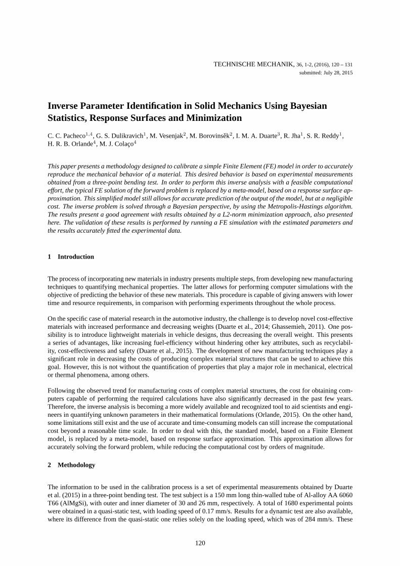
In order to extract information concerning the desired parameters from these experimental measurements, an in-verse analysis is performed. This type of analysis presents a close synergy between simulation and experimentalenvironments. The output of a mathematical model, obtained with a set of candidate values for the unknown pa-rameters, is compared with the experimental data in order to evaluate how well these values agree with each other.If this agreement is not good, then a new set of candidate values for the unknowns is selected in an ordinate fashionand re-tested. This iterative process is repeated as many times as necessary. For the purpose of establishing a linkwith the formal nomenclature presented in the literature, the prediction of the experimental values by selecting a setof candidate values for the desired parameters is calledforward problem, while the calculation of these parametersfrom previously obtained experimental measurements is calledinverse problem. In order to perform the desiredinverse analysis, it is paramount to be able to solve the forward problem and, in this work, the software chosen toperform this step was Abaqus software. The physical model, the simulation and the experimental environmentsare shown in Fig. 1.

(a) (b) (c)

Figure 1: Inverse problems framework: a) simulation, b) experimental environment and c) physical model.

The mathematical model is presented by Eqs. (1a)-(1e), whereb and σ contain the body forces and Cauchystress tensor in a momentum balance equation,ε stands for the strain andn is the outward normal unit vector.The boundary conditions are applied in the form of the vectorst, containing the loads applied atSt andup,containing the displacements applied atSu. The isotropic metal plasticity material model Eqs. (1c) (see Chapter4.3.2. of Simulia (2012)) is used with von Mises yield surface whereE stands for the Young’s modulus andν forPoisson’s ratio.σY is the yield stress which is given in dependence from the equivalent plastic strain. The isotropichardening with associated plastic flow is used in this model and all material properties are rate and temperature-independent. The constitutive equations are solved in an incremental-iterative procedure. The mid-side surface ofthe tube (diameter: 28 mm and length: 150 mm) has been discreti with shell FE with a thickness of 4 mm. Toreduce the computational time the double-symmetry has been used with boundary conditions shown in Fig. 1b (thegeometry of the support and loading cylinders has been included as well).

div σ + b = 0, in V (1a)

ε = L ∙ u (1b)

σ = σ(E, ν, σY ) (1c)

σ ∙ n = t, atSt (1d)

uSu = up, atSu (1e)

The unknown variables for this work are key material properties such as the Young’s modulus and the Poisson’sratio, as well a set of five plastic stresses that compose the non-linear behavior of the stress-strain curve in apiecewise fashion. These plastic stresses are associated to fixed plastic strains, shown in Tab. 1, that presents thissetup in Abaqus software.

The quality of the obtained estimates is highly dependent on how accurate the mathematical model representsthe phenomena of interest. When using numerical techniques to solve the forward problem, a very importantparameter is the grid size, representing a trade-off between accuracy and computational effort. However, sincetypical algorithms for solving inverse problems requires solving the forward problem several times, the slightestrefinement in the numerical grid is likely to increase the computational time beyond any feasible time scale. Thus,

121

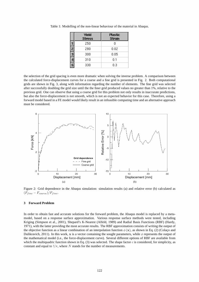
Table 1: Modelling of the non-linear behaviour of the material in Abaqus.

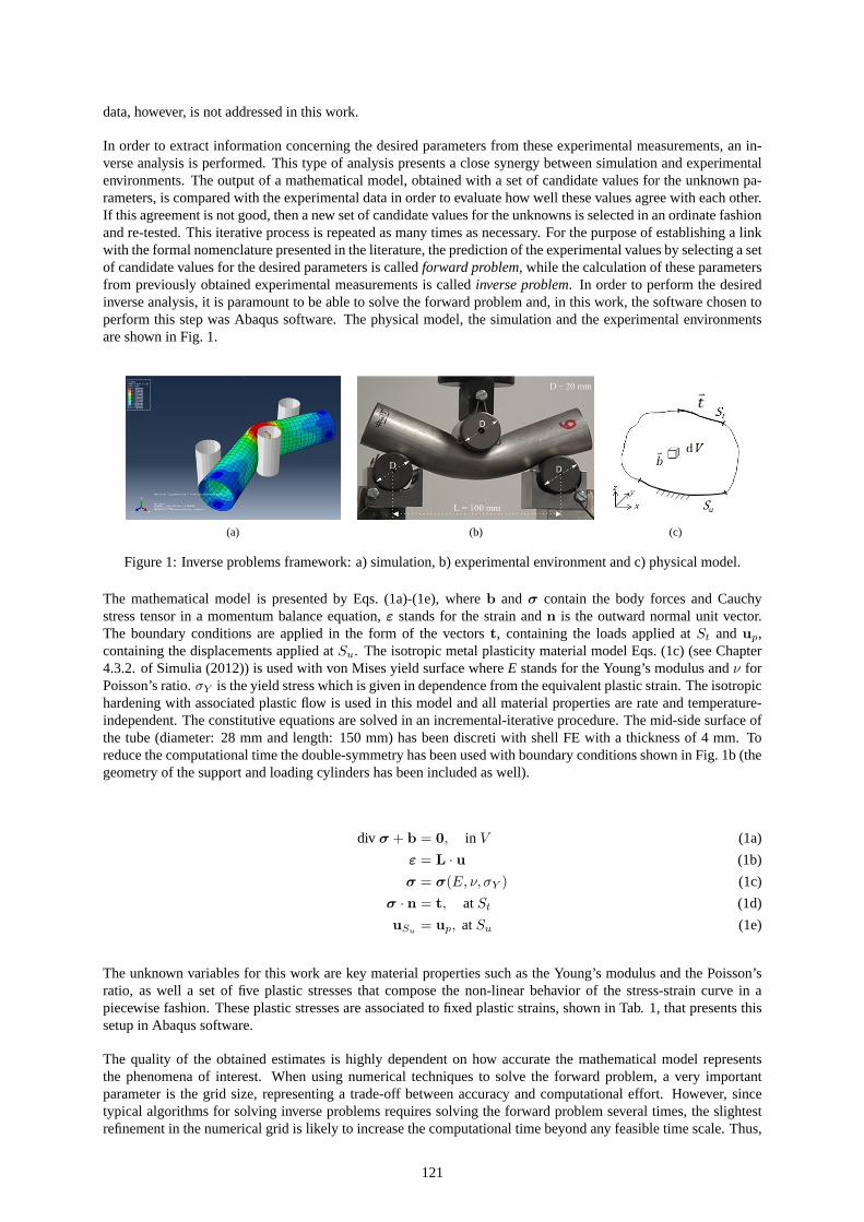
the selection of the grid spacing is even more dramatic when solving the inverse problem. A comparison betweenthe calculated force-displacement curves for a coarse and a fine grid is presented in Fig. 2. Both computationalgrids are shown in Fig. 3, along with information regarding the number of elements. The fine grid was selectedafter successfully doubling the grid size until the the finer grid produced values no greater than 1%, relative to theprevious grid. One can observe that using a coarse grid for this problem not only results in inaccurate predictions,but also the force-displacement is not smooth, which is not an expected behavior for this case. Therefore, using aforward model based in a FE model would likely result in an infeasible computing time and an alternative approachmust be considered.

(a) (b)

Figure 2: Grid dependence in the Abaqus simulation: simulation results (a) and relative error (b) calculated as(Ffine − Fcoarse)/Ffine.

3 Forward Problem

In order to obtain fast and accurate solutions for the forward problem, the Abaqus model is replaced by a meta-model, based on a response surface approximation. Various response surface methods were tested, includingKriging (Simpson et al., 2001), Shepard’s K-Nearest (Alfeld, 1989) and Radial Basis Functions (RBF) (Hardy,1971), with the latter providing the most accurate results. The RBF approximation consists of writing the output ofthe objective function as a linear combination of an interpolation functionφ (x), as shown in Eq. (2) (Colaco andDulikravich, 2011). In this work,x is a vector containing the sought parameters, whileφ represents the output ofthe mathematical model (i.e., the force-displacement curve). Several different options of RBF are available fromwhich the multiquadric function shown in Eq. (3) was selected. The shape factorc is considered, for simplicity, asconstant and equal to1/N, whereN stands for the number of measurements.

122

(a) (b)

Figure 3: Illustration of the computational grids generated in Abaqus for the (a) Coarse grid (∼1000 elements) and(b) Fine grid (∼30000 elements).

f(x) ' f(x) =K∑

k=1

wkφ(||x − xk||) (2)

φ(x) =√

xT x + c2 (3)

In order to allow for this RBF approximation to completely replace the Abaqus model, the weights,wk, need tobe calculated. This is done through a set of priorly known outputs of the Abaqus model, called thetraining set.These set, composed of results forK different simulated materials is organized in the form of a vectorf , while thevalues of the interpolation functions shown in Eq. (2) are calculated and organized in a matrixΦ. In other words,Φ is not the same asφ(x), but rather is composed of several values of it, organized in matrix form. With these twoquantities, the weights can be calculated by solving the linear system presented in Eq. (4).

Φw = f (4)

Having investigated the most accurate method for constructing a response surface, one must also address thedistribution of the points used to construct the approximation. In this work, the boundary conforming version ofSOBOL’s algorithm (Sobol, 1976) is used to uniformly distribute training points through a design space. Thisversion of the algorithm also allows for a user-specified number of points to be placed on the boundary of eachvariable, leading to the response surface to be accurate up to the variable bounds. Training of the response surfacewas performed by selecting a set ofK = 400 materials inside the pre-specified boundaries presented in Tab. 2. Inthis table, each Plastic stress is associated with a plastic strainεp, in agreement with Tab. 1.

Table 2: Bounds of design variables for the response surfaceapproximation.

Property Min. Max.

Young’s Modulus [GPa] 60 110Poisson’sRatio 0.3 0.4

Plastic Stress #1 [MPa] (εp = 0) 160 270Plastic Stress #2 [MPa] (εp = 0.02) 160 290Plastic Stress #3 [MPa] (εp = 0.05) 160 310Plastic Stress #4 [MPa] (εp = 0.10) 160 320Plastic Stress #5 [MPa] (εp = 0.30) 160 380

This approach has a big advantage in comparison with the usual FEM approach, because the calculation of theweights can be performed offline, that is, before the inverse analysis takes place. When the inverse problem solutionalgorithm starts, the forward problem is solved by just evaluating Eq. (2), resulting in an almost instantaneouscalculation.

123

4 Inverse Problem

In this section, the methodology selected to solve the inverse problem is described. Typically, the solution forsuch a problem is deeply related with the solution of the forward problem. The input of the proposed forwardproblem would include the material model and its parameters (the sought unknowns), boundary conditions andinitial conditions. The output of such analysis would the displacement field, from which a force-displacementcurve can be obtained. On the other hand, in an inverse analysis, the input consists of noisy measurements (inthis case, a set of force and displacement values) and the desired output are the sought material model parameters.Thus one can observe how obtaining an accurate solution of the forward model is paramount in order to obtainreliable estimates of the unknown parameters.

The solution of inverse problems within the Bayesian framework (Calvetti and Somersalo, 2007; Stuart, 2010;Idier, 2013; Gamerman, 1997). is a topic of ever increasing interest multiple fields of research. Both the develop-ment of more powerful computers and more efficient algorithms for solving the respective forward problems madebringing uncertainty quantification into the inverse analysis possible. As opposed to the classical regularizationtechniques, the result of the analysis is the quantification of the combined information priorly known and within theexperimental measurements. In this work, the selected methodology is based on the approach used for parameterestimation in a heat conduction problem (Orlande et al., 2007). The starting point in this framework is the set offour principles which is the foundation of this type of analysis (Kaipio and Somersalo, 2004):

1. All variables in the model are considered to be random variables;

2. The randomness of these variables describes the degree of information concerning their realizations;

3. This degree of information is coded in the form of probability distributions;

4. The solution of the inverse problem is the posterior probability distribution;

The posterior probability density function (pdf)π (x|y) represents the probability of a candidate value for theunknown vector of parametersx given the observationsy. According to Bayes’ theorem, shown in Eq. (5), theposterior pdf is proportional to two other functions. The first one is thelikelihoodpdf π (y|x), which provides theprobability density of obtaining a specific observationy given a candidate value for the unknown parametersx.The second term is theprior pdf π (x), which contains any knowledge on the unknown parameters that is availablebefore the inverse analysis takes place.

π (x|y) ∝ π (y|x) π (x) (5)

According to the fourth principle presented in the beginning of this section, the solution of the inverse problem isthe posterior pdf. This means that, in order to quantify the available information about the parameters of interest,this function must be quantified in terms of well-known statistical quantities. One useful example is the conditionalmean, given by Eq. (6).

xCM = E [x|y] =∫

RN

xπ (x|y) dx (6)

Although the definition of conditional mean shown above looks simple, its calculation can become rather com-plicated as the complexity of the posterior pdf increases. In this work, these difficulties results from high dimen-sionality and non-linearities. Therefore, an alternative approach, based on a Monte Carlo integration is selected.According to the weak law of large numbers, the sample average of an ensemble of particles that follows the pos-terior pdf converges in probability to the expected value ofπ (x|y) as the number of samples approaches infinity.Thus, the conditional mean given by Eq. (6) can be approximated by Eqs. (7) and (8), where a set ofM samplesx(i) of the sought parameter vectorx is used. The covariance matrix can be approximated in a similar fashion,by Eq. (9). Next, we describe the methodology selected to generate this set of samplesx(i), using the forwardproblem.

124

xCM = E [x|y] '1M

M∑

i=1

x(i) (7)

x(i) ∼ π (x|y) , i = 1, . . . ,M (8)

cov (x) '1

M − 1

M∑

i=1

[x(i) − xCM

] [x(i) − xCM

]T(9)

In practical terms, this approach implies in substituting the problem of calculating complex and high dimensionalnumerical integrals by the problem of sampling fromπ (x|y), in order to calculate the desired statistics. Bydefinition, any sampling technique will suffice in order to perform this task. Thus, several techniques designed forthis end can be found in the literature, including both basic sampling techniques, such as sampling by inversion,rejection and ratio of uniforms (Bishop, 2013) , and advanced ones, such as the MCMC (Gamerman, 1997).

In this work, the Metropolis-Hastings algorithm (Metropolis et al., 1953) was chosen to perform this task. This

algorithm constructs a Markov chain{x(i)}N

i=1from which it is possible to extract samples that follows the desired

pdf, also called theequilibrium distributionof the Markov chain. Thus, in order to use this algorithm, one needsto constructπ (x|y).

Before obtaining the posterior pdf, one must define theπ (y|x) andπ (x) pdf. The likelihood is considered to bea Gaussian pdf, given by Eq. (10). This choice of pdf implies in modelling the measurement errors as additive,Gaussian and with zero mean. Furthermore, these measurement errors are considered to be uncorrelated and havingthe same standard deviation, allowing the covariance matrix to be written in the form presented by Eq. (11). As forthe prior pdf, it is considered to be uniformly distributed throughout the parameter space.

π (y|x) ∝ exp[−1/2||y − f (x) ||2W−1

](10)

W = σ2I (11)

Another important feature that must be addressed in order to use the Metropolis-Hastings algorithm is defining theproposalpdf q

(x∗|x(i)

). This function represents the probability of sampling a specific candidate valuex∗ given

the last statex(i) of the Markov chain. In this work, this pdf was modelled as uniformly distributed aroundx(i),as shown in Eq. (12). This results in arandom-walk model, where the step size is adjusted by the quantityΔx.

x∗|x(i−1) ∼ U[x(i−1) − Δx,x(i−1) + Δx

](12)

The outcome of the Metropolis-Hastings algorithm is a Markov chain for which the posterior pdf is the equilibriumdistribution. Thus, in order to perform the Monte Carlo integration, one needs to extract i.i.d. samples from thischain. This is done by calculating the autocorrelation timeτj (Orlande, 2015), given by Eqs. (13)-(15). The desiredsamples can then be obtained by selecting one at eachmax τj .

τj = 1 + 2∞∑

k=1

ρjff (k) (13)

ρjff (k) =

Cjff (s)

Cjff (0)

(14)

Cjff (s) = cov

(x(i)

j ,x(i+s)j

)(15)

125

5 Results

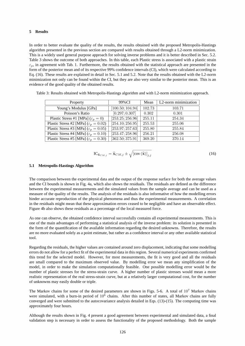
In order to better evaluate the quality of the results, the results obtained with the proposed Metropolis-Hastingsalgorithm presented in the previous section are compared with results obtained through a L2-norm minimization.This is a widely used general purpose approach for solving inverse problems and it is better described in Sec. 5.2.Table 3 shows the outcome of both approaches. In this table, each Plastic stress is associated with a plastic strainεp, in agreement with Tab. 1. Furthermore, the results obtained with the statistical approach are presented in theform of the posterior mean and of its respective 99% confidence intervals (CI), which were calculated according toEq. (16). These results are explained in detail in Sec. 5.1 and 5.2. Note that the results obtained with the L2-normminimization not only can be found within the CI, but they are also very similar to the posterior mean. This is anevidence of the good quality of the obtained results.

Table 3: Results obtained with Metropolis-Hastings algorithm and with L2-norm minimizationapproach.

Property 99%CI Mean L2-normminimization

Young’s Modulus [GPa] [100.50; 104.94] 102.73 103.71Poisson’sRatio [0.297; 0.307] 0.302 0.301

Plastic Stress #1 [MPa] (εp = 0) [253.25; 256.96] 255.11 254.34Plastic Stress #2 [MPa] (εp = 0.02) [254.10; 256.95] 255.53 255.06Plastic Stress #3 [MPa] (εp = 0.05) [253.97; 257.63] 255.80 255.84Plastic Stress #4 [MPa] (εp = 0.10) [253.47; 258.96] 256.21 256.08Plastic Stress #5 [MPa] (εp = 0.30) [362.50; 375.91] 369.20 370.14

ICxCM,j= xCM,j ±

√[cov(x)]j,j (16)

5.1 Metropolis-Hastings Algorithm

The comparison between the experimental data and the output of the response surface for both the average valuesand the CI bounds is shown in Fig. 4a, which also shows the residuals. The residuals are defined as the differencebetween the experimental measurements and the simulated values from the sample average and can be used as ameasure of the quality of the results. The analysis of the residuals is also informative of how the modelling errorshinder accurate reproduction of the physical phenomena and thus the experimental measurements. A correlationin the residuals might mean that these approximation errors ceased to be negligible and have an observable effect.Figure 4b also shows these residuals as a percentage of the local measured force.

As one can observe, the obtained confidence interval successfully contains all experimental measurements. This isone of the main advantages of performing a statistical analysis of the inverse problem: its solution is presented inthe form of the quantification of the available information regarding the desired unknowns. Therefore, the resultsare no more evaluated solely as a point estimate, but rather as a confidence interval or any other available statisticaltool.

Regarding the residuals, the higher values are contained around zero displacement, indicating that some modellingerrors do not allow for a perfect fit of the experimental data in this region. Several numerical experiments confirmedthis trend for the selected model. However, for most measurements, the fit is very good and all the residualsare small compared to the maximum observed value. By modelling error we mean any simplification of themodel, in order to make the simulation computationally feasible. One possible modelling error would be thenumber of plastic stresses for the stress-strain curve. A higher number of plastic stresses would mean a morerealistic representation of the real stress-strain curve, but at a relatively larger computational cost, for the numberof unknowns may easily double or triple.

The Markov chains for some of the desired parameters are shown in Figs. 5-6. A total of107 Markov chainswere simulated, with a burn-in period of106 chains. After this number of states, all Markov chains are fullyconverged and were submitted to the autocovariance analysis detailed in Eqs. (13)-(15). The computing time wasapproximately four hours.

Although the results shown in Fig. 4 present a good agreement between experimental and simulated data, a finalvalidation step is necessary in order to assess the functionality of the proposed methodology. Both the sample

126

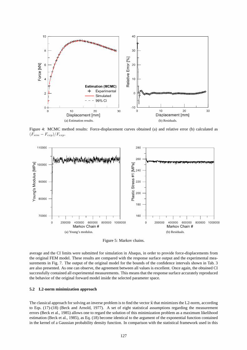
(a) Estimation results. (b) Residuals.

Figure 4: MCMC method results: Force-displacement curves obtained (a) and relative error (b) calculated as(Fsim − Fexp)/Fexp.

(a) Young’s modulus. (b) Residuals.

Figure 5: Markov chains.

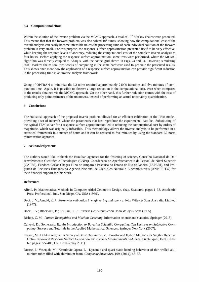
average and the CI limits were submitted for simulation in Abaqus, in order to provide force-displacements fromthe original FEM model. These results are compared with the response surface output and the experimental mea-surements in Fig. 7. The output of the original model for the bounds of the confidence intervals shown in Tab. 3are also presented. As one can observe, the agreement between all values is excellent. Once again, the obtained CIsuccessfully contained all experimental measurements. This means that the response surface accurately reproducedthe behavior of the original forward model inside the selected parameter space.

5.2 L2-norm minimization approach

The classical approach for solving an inverse problem is to find the vectorx that minimizes the L2-norm, accordingto Eqs. (17)-(18) (Beck and Arnold, 1977). A set of eight statistical assumptions regarding the measurementerrors (Beck et al., 1985) allows one to regard the solution of this minimization problem as a maximum likelihoodestimation (Beck et al., 1985), as Eq. (18) become identical to the argument of the exponential function containedin the kernel of a Gaussian probability density function. In comparison with the statistical framework used in this

127

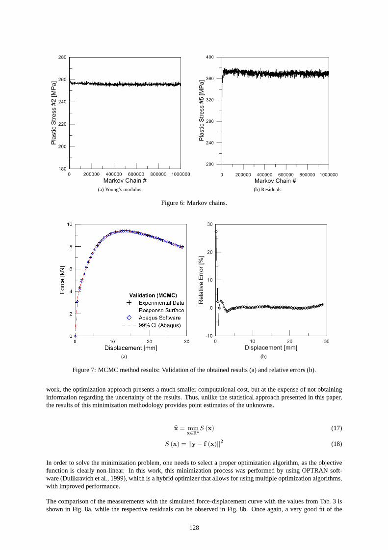
(a) Young’s modulus. (b) Residuals.

Figure 6: Markov chains.

(a) (b)

Figure 7: MCMC method results: Validation of the obtained results (a) and relative errors (b).

work, the optimization approach presents a much smaller computational cost, but at the expense of not obtaininginformation regarding the uncertainty of the results. Thus, unlike the statistical approach presented in this paper,the results of this minimization methodology provides point estimates of the unknowns.

x = minx∈Rn

S (x) (17)

S (x) = ||y − f (x)||2 (18)

In order to solve the minimization problem, one needs to select a proper optimization algorithm, as the objectivefunction is clearly non-linear. In this work, this minimization process was performed by using OPTRAN soft-ware (Dulikravich et al., 1999), which is a hybrid optimizer that allows for using multiple optimization algorithms,with improved performance.

The comparison of the measurements with the simulated force-displacement curve with the values from Tab. 3 isshown in Fig. 8a, while the respective residuals can be observed in Fig. 8b. Once again, a very good fit of the

128

experimental data can be noticed, leading to residuals similar to the ones obtained with the MCMC. However, asthere is no information regarding the uncertainty of the results, only point estimates are available at the end of theanalysis. The larger residual values at the edges of the x-axis are evidence of how the forward model struggles toreproduce the experimental measurements. Although these results are very satisfactory, if one desired to improvethem in order to obtain uncorrelated residuals, some upgrades in the physical model must be considered.

Finally, the results obtained with OPTRAN were also submitted to simulation in Abaqus software in order toevaluate the ability of the response surface in accurately reproducing the behavior of the original forward model.This result is presented in Fig. 9 where, once again, an excellent agreement between the response surface, Abaqussoftware and the experimental measurements was observed.

(a) Estimation results. (b) Residuals.

Figure 8: L2-norm minimization results: Force-displacement curves obtained (a) and relative error (b) calculatedas(Fsim − Fexp)/Fexp.

(a) (b)

Figure 9: L2-norm minimization results: Validation of the obtained results (a) and relative error (b) calculated as(Fsim − Fexp)/Fexp.

129

5.3 Computational effort

Within the solution of the inverse problem via the MCMC approach, a total of107 Markov chains were generated.This means that that the forward problem was also solved107 times, showing how the computational cost of theoverall analysis can easily become infeasible unless the processing time of each individual solution of the forwardproblem is very small. For this purpose, the response surface approximation presented itself to be very effective,while keeping the required levels of accuracy, reducing the computational cost of the complete inverse analysis tofour hours. Before applying the response surface approximation, some tests were performed, where the MCMCalgorithm was directly coupled to Abaqus, with the coarse grid shown in Figs. 2a and 3a. However, simulating5000 Markov chains took two weeks of computing in the same hardware used to generate the presented results.This shows once more how the application of a response surface approximation can provide significant reductionin the processing time in an inverse analysis framework.

Using of OPTRAN to minimize the L2-norm required approximately24000 iterations and five minutes of com-putation time. Again, it is possible to observe a large reduction in the computational cost, even when comparedto the results obtained via the MCMC approach. On the other hand, this further reduction comes with the cost ofproducing only point estimates of the unknowns, instead of performing an actual uncertainty quantification.

6 Conclusions

The statistical approach of the proposed inverse problem allowed for an efficient calibration of the FEM model,providing a set of intervals where the parameters that best reproduce the experimental data lie. Substituting ofthe typical FEM solver for a response surface approximation led to reducing the computational cost by orders ofmagnitude, which was originally infeasible. This methodology allows the inverse analysis to be performed in astatistical framework in a matter of hours and it can be reduced to five minutes by using the standard L2-normminimization approach.

7 Acknowledgements

The authors would like to thank the Brazilian agencies for the fostering of science, Conselho Nacional de De-senvolvimento Cientifico e Tecnologico (CNPq), Coordenaco de Aperfeicoamento de Pessoal de Nivel Superior(CAPES), Fundaco Carlos Chagas Filho de Amparo a Pesquisa do Estado do Rio de Janeiro (FAPERJ), and Pro-grama de Recursos Humanos da Agencia Nacional de Oleo, Gas Natural e Biocombustiveis (ANP/PRH37) fortheir financial support for this work.

References

Alfeld, P.: Mathematical Methods in Computer Aided Geometric Design. chap. Scattered, pages 1–33, AcademicPress Professional, Inc., San Diego, CA, USA (1989).

Beck, J. V.; Arnold, K. J.:Parameter estimation in engineering and science. John Wiley & Sons Australia, Limited(1977).

Beck, J. V.; Blackwell, B.; St.Clair, C. R.:Inverse Heat Conduction. John Wiley & Sons (1985).

Bishop, C. M.:Pattern Recognition and Machine Learning. Information science and statistics, Springer (2013).

Calvetti, D.; Somersalo, E.:An Introduction to Bayesian Scientific Computing: Ten Lectures on Subjective Com-puting. Surveys and Tutorials in the Applied Mathematical Sciences, Springer New York (2007).

Colaco, M.; Dulikravich, G.: A Survey of Basic Deterministic, Heuristic and Hybrid Methods for Single-ObjectiveOptimization and Response Surface Generation. In:Thermal Measurements and Inverse Techniques, Heat Trans-fer, pages 355–405, CRC Press (may 2011).

Duarte, I.; Vesenjak, M.; Krstulovic-Opara, L.: Dynamic and quasi-static bending behaviour of thin-walled alu-minium tubes filled with aluminium foam.Composite Structures, 109, (2014), 48–56.

130

Duarte, I.; Vesenjak, M.; Krstulovic-Opara, L.; Anzel, I.; Ferreira, J. M.: Manufacturing and bending behaviour ofin situ foam-filled aluminium alloy tubes.Materials & Design, 66, (2015), 532–544.

Dulikravich, G.; Martin, T.; Dennis, B.; Foster, N.: Multidisciplinary Hybrid Constrained GA Optimization. In:EUROGEN99-Evolutionary Algorithms in Engineering and Computer Science: Recent Advances and IndustrialApplications, chap. 12, pages 231–260, John Wiley & Sons, Inc. (1999).

Gamerman, D.:Markov Chain Monte Carlo: Stochastic Simulation for Bayesian Inference. Chapman & Hall/CRCTexts in Statistical Science, Taylor & Francis (1997).

Ghassemieh, E.: Materials in Automotive Application, State of the Art and Prospects. In:New Trends and Devel-opments in Automotive Industry, chap. 20, pages 365–394 (2011).

Hardy, R. L.: Multiquadric equations of topography and other irregular surfaces.Journal of Geophysical Research,76, (1971), 1905.

Idier, J.:Bayesian Approach to Inverse Problems. ISTE, Wiley (2013).

Kaipio, J. P.; Somersalo, E.:Statistical and Computational Inverse Problems. Springer Science+Business Media,Inc (2004).

Metropolis, N.; Rosenbluth, A. W.; Rosenbluth, M. N.; Teller, A. H.; Teller, E.: Equation of State Calculations byFast Computing Machines.The Journal of Chemical Physics, 21, (1953), 1087–1092.

Orlande, H. R. B.: The use of techniques within the Bayesian framework of statistics for the solution of inverseproblems. In:Metti 6 Advanced School: Thermal Measurements and Inverse Techniques, Biarritz (2015).

Orlande, H. R. B.; Colaco, M. J.; Dulikravich, G. S.: Approximation of the likelihood function in the bayesiantechnique for the solution of inverse problems.Inverse Problems, Design and Optimization Symposium.

Simpson, T. W.; Mauery, T. M.; Korte, J.; Mistree, F.: Kriging models for global approximation in simulation-based multidisciplinary design optimization.AIAA Journal, 39, 12, (2001), 2233–2241.

Simulia: Abaqus Online Documentation - Theory Manual(2012).

Sobol, I.: Uniformly distributed sequences with an additional uniform property.USSR Computational Mathematicsand Mathematical Physics, 16, 5, (1976), 236–242.

Stuart, A. M.: Inverse problems: A Bayesian perspective.Acta Numerica, 19, (2010),451–559.

Address:1MAIDROC Laboratory, EC 3474, Department of Mechanical and Materials Engineering, Florida InternationalUniversity, 10555 West Flagler Street, Miami, Florida 33174, USAE-mail: cesar.pacheco@poli.ufrj.br dulikrav@fiu.edu rjha001@fiu.edu sredd001@fiu.edu

2Department of Mechanical Engineering, University of Maribor, Maribor, SloveniaE-mail: matej.vesenjak@um.si matej.borovinsek@um.si

3Department of Mechanical Engineering, University of Aveiro, TEMA, Aveiro, PortugalE-mail: isabel.duarte@ua.pt

4Department of Mechanical Engineering, COPPE, Federal University of Rio de Janeiro - UFRJ, BrazilE-mail: helcio@mecanica.ufrj.br colaco@ufrj.br

131