formula sae cooling system design · fsae rules ... figure 5. this fsae team has installed their...
TRANSCRIPT

Formula SAE Cooling System Design
By
Lisa Van Den Berg, Student
Brandon Lofaro, Student
Mechanical Engineering Department
California Polytechnic State University
San Luis Obispo
2014

1
Statement of Confidentiality
The complete senior project report was submitted to the project advisor and sponsor. The results
of this project are of a confidential nature and will not be published at this time.

2
Statement of Disclaimer
Since this project is a result of a class assignment, it has been graded and accepted as fulfillment
of the course requirements. Acceptance does not imply technical accuracy or reliability. Any use
of information in this report is done at the risk of the user. These risks may include catastrophic
failure of the device or infringement of patent or copyright laws. California Polytechnic
University at San Luis Obispo and its staff cannot be held reliable for any use or misuse of the
project.

3
Table of Contents
Table of Figures .............................................................................................................................. 5
Table of Tables ............................................................................................................................... 8
Executive Summary ........................................................................................................................ 9
Chapter1: Introduction .................................................................................................................. 10
1. Sponsor Background and Needs ........................................................................................ 10
2. Formal Problem Definition ................................................................................................ 10
Chapter 2: Background ................................................................................................................. 11
1. FSAE Rules ........................................................................................................................ 11
2. Initial Meetings .................................................................................................................. 11
3. Engine Used on the Car ..................................................................................................... 14
4. Types of Radiators ............................................................................................................. 14
5. Radiator Installation in FSAE Application ........................................................................ 15
6. Fan Sizing .......................................................................................................................... 16
7. Measuring the Mass Flow Rate of Air ............................................................................... 17
8. Effectiveness-NTU Method of Determining Heat Transfer Characteristics ...................... 20
9. Literature Review for Testing Procedure Formulation ...................................................... 21
10. Equipment Available at Cal Poly ................................................................................... 22
11. Test Equipment Requirements ....................................................................................... 23
Chapter 3: Design Development ................................................................................................... 25
1. Conceptual Designs ........................................................................................................... 25
2. Concept Selection .............................................................................................................. 29
3. Supporting Preliminary Analysis ....................................................................................... 30
Chapter 4: Final Design Description............................................................................................. 32
1. Overall Description- Testing.............................................................................................. 32
2. Detailed Design Description- The Test Section................................................................. 33
3. Cost Analysis ..................................................................................................................... 36
4. Geometry, Material, and Component Selection ................................................................. 36
5. Manufacturing Drawings ................................................................................................... 38
6. Maintenance and Repair Considerations ........................................................................... 38

4
Chapter 5: Product Realization ..................................................................................................... 39
1. Description of Design Iteration .......................................................................................... 39
2. Manufacturing Process....................................................................................................... 39
Chapter 6: Testing ......................................................................................................................... 43
1. Test Descriptions ............................................................................................................... 43
2. Safety Considerations ........................................................................................................ 61
3. Test Results ........................................................................................................................ 62
4. Specification Verification Checklist or DVP&R ............................................................... 72
Chapter 7: Conclusions and Recommendations ........................................................................... 74
Appendix A: Gantt Chart .............................................................................................................. 76
Appendix B: Decision Matrices, QFD .......................................................................................... 77
Appendix C: Fan Sizing Program Calculations ............................................................................ 79
Appendix D: Heater Sizing Program ............................................................................................ 80
Appendix E: Temperature Effects on Manometer Reading .......................................................... 82
Appendix F: Cost Analysis Table ................................................................................................. 83
Appendix G: Bills of Materials & Manufacturing/Vendor Drawings .......................................... 84
Appendix H: Excel Program Tables ........................................................................................... 135
Appendix I: Testing Flowchart ................................................................................................... 140
Appendix J: References .............................................................................................................. 141

5
Table of Figures
Figure 1. Diagram of a typical dynamometer coupled to an engine ............................................ 12
Figure 2. Histogram describing the number of instances when the car travels at a particular
speed ............................................................................................................................................. 13
Figure 3. Yamaha WR450F engine, used by Cal Poly FSAE in 2013 .......................................... 14
Figure 4. Diagrams of single pass, downflow (left) and dual pass, crossflow (right) radiators .. 15
Figure 5. This FSAE team has installed their radiator such that it is side-mounted at an angle 15
Figure 6. Typical fan-system curve ............................................................................................... 16
Figure 7. Meriam 50MC2-04 LFE................................................................................................ 17
Figure 8. Diagram of a pitot-static tube in a duct with air flow .................................................. 18
Figure 9. Example of the way an array of measurements may be taken with a pitot-static tube . 18
Figure 10. A venturi section with a liquid column manometer..................................................... 19
Figure 11. AAR radiator flowbench schematic............................................................................. 25
Figure 12. Conceptual design used for radiator testing, LFE configuration ............................... 26
Figure 13. Conceptual design used for radiator testing, contraction area configuration ........... 26
Figure 14. Swirling and vortexing that occurs without gradual contraction ............................... 27
Figure 15. Conceptual design used for radiator testing, pressure rise across fan ...................... 27
Figure 16. Conceptual design used for radiator testing, radiator interfaces with test section on
existing wind tunnel ...................................................................................................................... 28
Figure 17. Unobstructed view of the test section .......................................................................... 29
Figure 18. View of the thumbscrew for height adjustment of the radiator support and steel tube
static pressure ports ...................................................................................................................... 29
Figure 19. Plot of the effect of exit air temperature on manometer liquid column height
differential ..................................................................................................................................... 31
Figure 20. The radiator will be secured between two pieces of the new test section ................... 34
Figure 21. Method of mounting brown expansion section to adjacent downstream wind tunnel
section ........................................................................................................................................... 34
Figure 22. Method of mounting downstream piece of test section to brown expansion section .. 35
Figure 23. Method of mounting upstream piece of test section to adjacent section of the wind
tunnel............................................................................................................................................. 35
Figure 24. SolidWorks model of the test section depicts the use of closed-cell foam gasket
material and metal tube location .................................................................................................. 35
Figure 25. First step: fasten wood brackets to each side of ducting ............................................ 40
Figure 26. Second step: construct duct portion ............................................................................ 40
Figure 27. Third step: attach each part of the flanges ................................................................. 41
Figure 28. SolidWorks model of the finished test section ............................................................. 41
Figure 29. Experimental setup for Test 1 ..................................................................................... 44
Figure 30. Example of what the plot generated with completion of Test 1 may look like ............ 45
Figure 31. Experimental setup for Test 2 ..................................................................................... 46

6
Figure 32. Example of what the plot generated with completion of Test 2 may look like ............ 47
Figure 33. Plot of results from completion of Test 3 .................................................................... 49
Figure 34. Experimental setup for Test 4- ensuring the core is airtight ...................................... 50
Figure 35. Experimental setup for Test 4- securing the radiator between the two test section
pieces............................................................................................................................................. 50
Figure 36. Experimental setup for Test 4- connecting the tubing to the static pressure ports on
the test section ............................................................................................................................... 51
Figure 37. Orientation of the pitot-static tube in the test section during Test 4........................... 52
Figure 38. Plot of results from Test 3- average air velocity and mass flow rate associated with
static pressure drop....................................................................................................................... 52
Figure 39. Plot of results from Test 3- static pressure associated with mass flow rate of air
through the core ............................................................................................................................ 53
Figure 40. Experimental setup for Test 5 ..................................................................................... 55
Figure 41. Heating water using immersion heaters ..................................................................... 56
Figure 42. Heat rejection rate as a function of water and air mass flow rates- water mass flow
rate on the x-axis ........................................................................................................................... 58
Figure 43. Heat rejection rate as a function of water and air mass flow rates- air mass flow rate
on the x-axis .................................................................................................................................. 58
Figure 44. Predicted relationship between cooling fluid mass flow rate and crank speed from
Excel program ............................................................................................................................... 63
Figure 45. Predicted relationship between rate of heat rejection to the cooling fluid and crank
speed from Excel program ............................................................................................................ 64
Figure 46. Measured relationship between the average air velocity and mass flow rate of air
through the core and car speed .................................................................................................... 65
Figure 47. Core of radiator borrowed from the formula team ..................................................... 66
Figure 48. C&R racing radiator, notice damaged fins in the top right hand corner of the exposed
area ............................................................................................................................................... 66
Figure 49. C&R racing radiator, undamaged fins ....................................................................... 66
Figure 50. Calibration curve for radiator from formula team- average velocity and mass flow
rate of air through core as a function of static pressure drop ...................................................... 68
Figure 51. Calibration curve for C&R radiator- average velocity and mass flow rate of air
through core as a function of static pressure drop ....................................................................... 68
Figure 52. System curve for radiator borrowed from formula team ............................................ 69
Figure 53. System curve for C&R radiator .................................................................................. 69
Figure 54. Heat rejection as a function of the mass flow rate of air, radiator borrowed from
formula team ................................................................................................................................. 71
Figure 55. Heat rejection as a function of the mass flow rate of air, C&R radiator ................... 71
Figure 56. Heat rejection as a function of the mass flow rate of water, radiator borrowed from
formula team ................................................................................................................................. 72
Figure 57. Heat rejection as a function of the mass flow rate of water, C&R radiator ............... 72

7
Figure 58. Plumbing at radiator outlet- thermocouple and valve .............................................. 123
Figure 59. Plumbing at pump discharge to couple pump discharge fitting to hose ................... 130
Figure 60. Screenshot of “Cooling Water Mass Flow Rate" spreadsheet in Excel program .... 135
Figure 61. Screenshot of "Heat Rej. to Water" spreadsheet from Excel program ..................... 136
Figure 62. Screenshot of "Core Air Flow" spreadsheet from Excel program ............................ 137
Figure 63. Screenshot of "Core Pressure Drop" spreadsheet from Excel program .................. 138
Figure 64. Screenshot of "Heat Rej. from Radiator" spreadsheet from Excel program ............ 139
Figure 65. Flowchart to guide user through application of test results ..................................... 140

8
Table of Tables
Table 1. Description of each piece of wood that would be used in the construction of the test
section ........................................................................................................................................... 40
Table 2. Array of measurements of air velocity through core, car speed = 20mph ..................... 64
Table 3. Array of measurements of air velocity through core, car speed = 30mph ..................... 64
Table 4. Array of measurements of air velocity through core, car speed = 50mph ..................... 64
Table 5. Array of measurements of air velocity through core, car speed = 40mph ..................... 64
Table 6. Array of measurements of air velocity through core, car speed = 60mph ..................... 64
Table 7. Array of air velocity measurements behind the radiator in the wind tunnel ducting,
formula team's radiator core ........................................................................................................ 67
Table 8. Array of air velocity measurements behind the radiator in the wind tunnel ducting, C&R
racing radiator core ...................................................................................................................... 67
Table 9. Water mass flow rates at different pump speeds for each radiator ................................ 70
Table 10. Gantt chart describing project timeline ........................................................................ 76
Table 11. Decision matrix used in concept selection .................................................................... 77
Table 12. QFD for use of the ME Thermal Science Lab wind tunnel to perform radiator
characterization testing ................................................................................................................ 78
Table 13. Cost of each component used throughout the project- "cost" column includes 8.0% tax
....................................................................................................................................................... 83
Table 14. Bill of materials corresponding to above figure ......................................................... 123
Table 15. Bill of materials corresponding to above figure ......................................................... 130

9
Executive Summary
The overall objective of this senior project is to develop, via testing and analysis, a guided
process that will aid the Cal Poly Formula SAE team in designing their cooling system. More
specifically, a set of designed tests will yield the results necessary in determining a combination
of fan and radiator that will achieve appropriate cooling.
A test section that has the capability of interfacing with both the wind tunnel in the Thermal
Science Lab and a radiator will be used to facilitate the necessary experiments. The wind tunnel
is powered by fan controlled by a variable frequency drive that can induce a range of air flow
rates through the duct and radiator. Five tests will be performed, whose goals are as follows:
1. Determine mass flow rate of the cooling water as a function of the crank shaft rotational
speed.
2. Determine heat rejected from the engine to the cooling water as a function of crank shaft
rotational speed.
3. Determine the mass flow rate of air through the core as a function of car speed.
4. Determine static pressure drop of the air across the radiator core at varying air mass flow
rates.
5. Determine the heat rejection rate associated with a test radiator as a function of both the
mass flow rate of air through the core and the mass flow rate of cooling water.
These tests will develop relationships that will ultimately allow the formula team to predict the
heat rejection necessary at every car speed as well as the ability of a particular radiator to reject
heat at those speeds. A guided process will be presented that will aid the team in designing the
cooling system to be used on the formula competition car. By performing these tests, the FSAE
team can choose an appropriate radiator type and face area for the racecar’s specific cooling
needs each year. This process will allow the team to minimize the radiator’s size and optimize
cooling to increase performance.
The following report will detail background information regarding a car’s cooling system, a
description of conceptual designs, the final design process, the test procedures and finally sample
results produced via testing.

10
Chapter1: Introduction
1. Sponsor Background and Needs
Cal Poly’s Formula SAE team needs a method of correctly and easily sizing the radiator for their
racecar each year. Currently, radiators are chosen based on previous radiators that the team has
used that have adequately cooled the engine but without the analysis of the cooling system to
correctly choose the face area, type of radiator and manufacturer of the radiator for each car.
Although the cooling systems in the past have worked, they lack true engineering justification. In
developing this test method, we will aid the FSAE team in the process of choosing a radiator and
fan to minimize the size and weight of the radiator for their application.
2. Formal Problem Definition
The Formula SAE team at Cal Poly sponsored us in our development of a process that will aid
them in designing the formula car’s cooling system each year. In the past, there has been no
formal engineering design that has gone into developing the cooling system, so we have
developed a test procedure that will guide them through a design process that is based on
engineering principles in fluids and heat transfer.

11
Chapter 2: Background
Background research spanned the following topics: the FSAE rules regarding keeping the engine
cool, the components and plumbing used in cooling systems, methods of sizing a radiator, the
variables that affect the engine cooling and how these variables can be manipulated in the
system, as well as measurement techniques. A detailed explanation of the background research
that was performed follows.
1. FSAE Rules
Because we are working with FSAE, the cooling system of the car must comply with the FSAE
Rules. In the 2013 FSAE Rules, the specifications relating to the cooling system are that there
must be a “firewall to separate the driver compartment from all the components of the fuel
supply, the engine oil, the liquid cooling systems and any high voltage system” (T4.5.1.
2013fsaerules), the “cooling or lubrication system must be sealed” (T8.2.1 2013fsaerules), “any
catch can on the cooling system must vent through a hose with a minimum internal diameter of 3
mm” (T8.2.4 2013fsaerules), and “no power device may be used to move or remove air from
under the vehicle except fans designed exclusively for cooling” (T9.4 2013fsaerules). Also,
“water-cooled engines must only use plain water. Electric motors, accumulators or HV
electronics can use plain water or oil as the coolant. Glycol-based antifreeze, “water wetter”,
water pump lubricants of any kind, or any other additives is strictly prohibited” (T8.1
2013fsaerules). Thus, the details within the cooling system such as the number, size, type, and
orientation of the radiators or whether oil coolers and fans are necessary are left to the team to
decide. This leaves our team a lot of freedom to change and test some of these variables in order
to optimize the system.
2. Initial Meetings
We first met with John Waldrop at the Hangar on the California Polytechnic University campus
who gave us an introduction to the FSAE team, showed us the car that would be used at
competition in June 2013, showed us the current cooling system components, informed us of
what testing they have done already, and described some of the significant variables. John
described the dynamometer and the way it worked to measure the torque at different speeds and
tune the engine by determining a correct gas/air mixture for the combustion process. The engine
is cooled with a radiator-fan combination on the dynamometer. A dynamometer, or “dyno,” is an
instrument used to measure torque. In the case of the Formula SAE team, it is used as a way of
tuning their engine and will be used in our testing as described in Test Descriptions (Chapter 6,
Section 1). A diagram of a typical dyno can be observed in Figure 1 below. In the figure, the
engine’s drive shaft is coupled to a shaft on the dyno. A tachometer is used to measure the

12
rotational speed of the shaft and the torque arm, which is generally resisted with some sort of
fluid inside the housing, is used to measure torque. The torque is displayed on the scale and the
housing is supported in trunnion bearings.
Figure 1. Diagram of a typical dynamometer coupled to an engine
The test setup on the wind tunnel will mimic heat generated in the engine by using a hot water
source in the lab to fill the radiator. The water will need to be 180°F because when the water
flowing into the radiator reaches this temperature, the radiator fan on the car is set to turn on to
increase heat rejection and maintain this inlet temperature. We also met with Matt Roberts and
Eric Griess (two engine specialists on the FSAE team) to determine specific requirements for our
project proposal and gain some general knowledge regarding the engine.
Information on the FSAE car for June 2013 race from John Waldrop and Matt Roberts:
The fuel is gas
The coolant is water
Engine: Yamaha WR450F from 2003
Optional use of a turbo-charger
They provided a histogram to show the number of occurrences of the various speeds of
the racecar during a typical race. Refer to Figure 2.
The fan turns on when the temperature of the water entering the engine is greater than or
equal to 180 °F, and the fan turns off when the water entering the engine reaches 160°F.
The temperatures are measured within 6-12 inches before and after the engine (we can
assume there is negligible heat loss between the inlet/outlet of the engine’s cooling
system and where the temperature is measured).
The water pump is engine-driven
13
The FSAE team provided a histogram (see Figure 2) which describes the number of instances
when the car travels at a particular speed (in ft/s) over the course of the autocross event. This is
important because we can see the range of speeds spans a minimum speed of 35 ft/s to a
maximum speed of 95 ft/s and that a speed of 40 ft/s occurs most often in a typical race. This
will aid the team in choosing a design point which correlates to a particular car speed where they
will perform the guided radiator sizing process. During this process, they will be able to measure
the heat transferred from the engine to the cooling water over a range of mass flow rates of air
through the radiator core. It is important to realize that the speed of the car is not equal to the
average speed of the air that will move through the radiator plane due to the effects of friction
and drag in the radiator core. A method of developing relationship between the two to account
for the air velocity changes through the radiator core will be provided.
Figure 2. Histogram describing the number of instances when the car travels at a particular speed
We also had some helpful meetings with Cal Poly Professors Patrick Lemieux, John Fabijanic,
Kim Shollenberger, and Glen Thorncroft. From these meetings, we came up with a list of
variables that should be considered. These variables are as follows:
Mass flow rate of the water and air
When in the race (idle or high speed) is the engine the hottest
Type of radiator: Downflow/Cross-flow
Aluminum/Brass/Copper Core and the difference it makes for heat transfer
Orientation of the Radiator (heat transfer or packaging reasons)
Number of radiators
Fan (how to size, when necessary, how many, where placed)
Ducting in and out of the radiator (how diffusion affects the flow)
Pressure Drop Across the Radiator/Rise across the Fan
Accuracy of the equipment used

14
3. Engine Used on the Car
The engine used on the 2013 formula car was a 2003 Yamaha WR450F engine, which is a 40-
horsepower, single-cylinder, water-cooled, engine. As in almost all ground vehicle engines, the
engine is cooled using a radiator, where the cooling water flows through canals in the engine to
remove heat, then heat is transferred to the air when the cooling water flows through the radiator
core. The engine from a very similar 2007 model of the same dirt bike is depicted in Figure 3
below. The engine and the tip of the bottom tank of one of the radiators can be observed.
The method for sizing the radiator via testing will allow the formula team to size their radiator in
the event that they decide to use a different engine. For instance, they could use the engine from
a Honda CBR600F4i or CBR900RR. Honda’s CBR600F4i is a 90.1-hp, 4-cylinder engine and
Honda’s CBR900RR engine is 128-hp and 4-cylinder as well. In this case, it is predictable that
more heat would need to be rejected from each of these engines because they would produce
more waste heat. This is due to the fact that the waste heat produced by the engine is
proportional to the power that the engine produces. The process for sizing the radiator or
radiators that will be provided allows the team to take measurements to determine the amount of
heat that their engine rejects to the cooling water. Similarly, if the team decides to use a
turbocharger and oil cooler, more heat would need to be rejected from the system.
4. Types of Radiators
In the recent past, the FSAE team has used dirt bike engines to power their cars, and they have
used the OEM radiators that were used with the corresponding engine on the stock dirt bike. In
knowing how much heat transfer area the radiator needs to have to achieve adequate cooling, the
team can get more creative with the types of radiators they use. Radiators exist as either
Figure 3. Yamaha WR450F engine, used by Cal Poly FSAE in 2013
Radiator Outlet

15
crossflow or downflow radiators. A crossflow radiator has tanks on the left and right sides of the
radiator core and the cooling fluid travels parallel to the ground. Conversely, a downflow
radiator has tanks above and below the core and cooling fluid moves down towards the ground
through the core. In terms of performance, it is believed that there is no real difference between
the two types of radiators. Radiators also exist as single or dual pass radiators. In a single pass
radiator, the cooling fluid crosses the core once, while it crosses the core twice in a dual pass
radiator. Figure 4 depicts these characteristics. Typically, the team uses single pass radiators
which are more conventional, generally cheaper, and good for low flow/low pressure pumps. The
dual pass radiators are typically used for higher flow/higher pressure pump systems where a
single pass would not cool the coolant enough and a second pass is necessary.
5. Radiator Installation in FSAE Application
There are no FSAE regulations
concerning where to mount the
radiators or how many radiators to
use, but typically, the radiators are
side-mounted as depicted in Figure
5. They are often mounted at an
angle, but this is only a product of
packaging concerns. The angle at
which they are mounted should be
minimized because the air
streamlines won’t be guided evenly
through the tubes and there can be
uneven cooling across the radiator.
In the case of the 2013 Cal Poly
FSAE car, the two relatively smaller OEM radiators, have been side-mounted. It is also worth-
Figure 4. Diagrams of single pass, downflow (left) and dual pass, crossflow (right) radiators
Figure 5. This FSAE team has installed their radiator such that it is side-
mounted at an angle

16
while to note that when two radiators are used, they can be connected either in parallel or series.
It may be more efficient to connect them in parallel because high temperature cooling water
directly from the engine would flow to both radiators as opposed to having lower temperature
water flow to one of the radiators. The larger temperature gradient between cooling air and hot
water yields greater heat transfer. However, the distribution of the coolant must be split evenly to
both radiators to be effective, which is difficult to accomplish and risky as well. If the amount of
cooling fluid supplied to each radiator is not split evenly, it is possible that one radiator could be
doing almost none of the cooling in which case, the engine is at risk of overheating. As a result,
it is most common to connect two radiators in series in this application.
6. Fan Sizing
In a manner similar to a pump, a fan can pull or push air so
that it travels at a flow rate specific to a pressure drop. That
pressure drop is a product of the system design, and the
system pressure drop varies with the velocity of the flow. As
a result each fan-system combination has an equilibrium
point at which it will operate, as depicted in Figure 6. The
figure also shows a stall region where the flow separates
from the fan blades, which create vortices. These vortices
result in a back pressure, which is reflected in the figure.
The formula team will be able to determine the static
pressure drop across the radiator so that they can choose a fan, based on the manufacturer’s fan
curve, if they decide to use one.
Initially, when a flow bench was going to be built to facilitate testing, an estimate the system
pressure loss (losses due to ducting, duct components, and radiator core) was needed to size the
fan that would be used on the flow bench. We were provided a sample data point which indicated
the static pressure drop across a radiator core at a given speed: 50 ft/s and 57 psi pressure drop.
With this data, the loss coefficient of a typical radiator core could be estimated. In estimating the
major losses in the ducting and minor losses in the duct components at the maximum speed at
which the flow bench would be operated, we could choose a fan. The fan should have been able
to operate such that air would flow at the necessary maximum speed and overcome the
calculated system back pressure.
When we decided to conduct testing on the wind tunnel in the Thermal Science Lab, we assumed
that the fan on the wind tunnel would be adequate. That wind tunnel is capable of pulling air at a
Figure 6. Typical fan-system curve

17
velocity of up to 200 mph with no added loss elements in the ducting. We concluded that it
would be adequate to get our desired air speeds.
7. Measuring the Mass Flow Rate of Air
It is important to be able to measure the mass flow rate of the air in the wind tunnel duct because
heat transfer is highly dependent on the mass flow rate of the fluids involved. Once the average
velocity of the flow is determine, it is very easy to determine the mass flow rate of the fluid. It
will be assumed that air density is constant as it pertains to the application of flow through a hot
radiator. Proof of the validity of this assumption is described in Supporting Preliminary Analysis
(Chapter 3, Section 3). The mass flow rate of air is determined using the equation below:
�� = 𝜌𝑣𝐴
where �� is the mass flow rate of the air, ρ is the density of air, V is the average velocity of the
air through the duct, and A is the cross-sectional area of the duct. We assume the duct area is
equal to the face area of radiator tested if the radiator is mounted normal to the duct without any
air leaks around the radiator. The mass flow rate is conserved before and after the radiator as
well as before and after the fan. The velocity can be measured with different methods and
instruments, each with different accuracies. Some of these methods are as follows.
Method 1: Laminar Flow Element (LFE)
In an LFE, the static pressure drop is measured across a loss element with a calculated loss
coefficient. With the, loss coefficient, k, the static pressure drop, Δp and the density of the fluid,
the following equation can be used to find the average velocity of the air.
𝛥𝑝 = 𝑘0.5𝜌𝑣2
Laminar flow elements can be a very accurate method
of measuring air velocity in a duct. Cal Poly has two
LFE’s in the storage room in the Thermal Science
Lab, one of which can be interfaced with the wind
tunnel in the lab. The LFE that can be interfaced with
the wind tunnel is depicted in Figure 7. The two LFEs
are both made by Meriam. The smaller LFE (from
Figure 7) with part number 50MC2-04, is
approximately 4” in diameter at the inlet and outlet
and can measure flow rates up to 400 CFM. The Figure 7. Meriam 50MC2-04 LFE
(2)
(1)

18
larger LFE, with part number 50MC2-08, is approximately 8” in diameter at the inlet and outlet
and can measure flow rates up to 2200 CFM.
It was determined that the LFE would not be used during testing because it is very likely that it
needed to be calibrated. Further, it is typically used to measure flow rates that are less than 2 m/s,
which is not adequate in the case of the necessary test procedure.
Method 2: Pitot-Static Tube Array to produce Average Velocity
An array of pitot-static tube readings can be used to produce an average air velocity through the
core of the radiator. Pitot-static tubes measure both the total pressure and static pressure using to
separate ports on the pitot tube. In general, pitot static tubes are composed of two separate,
concentric tubes: one which measures static
pressure with a port perpendicular to the flow, and
one which measures total pressure parallel to the
flow. This is illustrated in Figure 8 on the right.
The digital readout that the pitot-static tube is
connected to can then use the static pressure (P1 in
the figure), total pressure (P2 in the figure), and
fluid density to deduce the dynamic pressure and
the velocity component of the dynamic pressure
that follows. This is obtained theoretically via
the following equation.
𝑣 = √2(𝑝𝑡 − 𝑝𝑠)
𝜌
A pitot-static tube only has the ability to determine the velocity
of the flow along a streamline. It is highly unlikely that the
velocity of the flow will be the same over the entire face of the
radiator core. Due to the fact that the goal is to eventually
determine the mass flow rate of air through the radiator core, an
array of measurements will need to be taken and averaged to
determine an average velocity of air through the core. This array
of measurements should be taken in a manner similar to the one
shown in Figure 9.
There are some drawbacks involved in using this method. First,
the pitot-static tube needs to be oriented so that the port that
measures total pressure needs to be oriented so that it is parallel
to the flow along a streamline. This is difficult to do even in developed flow where the flow is
Figure 8. Diagram of a pitot-static tube in a duct with air
flow
Figure 9. Example of the way an array
of measurements may be taken with a pitot-static tube
(3)

19
uniform and flowing along one axis in the duct. Second, because the pitot-static tube would be
used behind the radiator, the flow may not be developed until well after it has passed through the
radiator core.
Method 3: Pressure Differential in Venturi Section
Using a Venturi section is a simple and fairly accurate way of determining the mass flow rate of
the airflow in a duct directly, as opposed to determining the velocity, then using the velocity to
find the mass flow rate according to Equation 1. A Venturi, or contraction area in the duct, can
be used to find the velocity of the air through the pressure drop from the large to small diameter
cross sections. This is illustrated in Figure 10 below.
Figure 10. A venturi section with a liquid column manometer
A manometer is used to determine the difference in pressure between the two sections. The
difference in liquid column heights is then used to determine the differential pressure (P1 – P2
where P1 and P2 are as they appear in Figure 10). This is accomplished using the following
equation.
ℎ = 𝑃1 − 𝑃2
𝛾
Once the pressure differential has been determined, the following equation can be used to
determine the mass flow rate of the air in the duct.
𝑄 = 𝐴1√2
𝜌×
(𝑃1 − 𝑃2)
(𝐴1
𝐴2⁄ )2 − 1
= 𝐴2√2
𝜌×
(𝑃1 − 𝑃2)
1 − (𝐴2
𝐴1⁄ )2
The caveat to using this method is that the Venturi section requires a gradual expansion after the
reduced area region, or the flow will separate from the duct walls. This is not something that
would be practical to install on the wind tunnel in the Thermal Science Lab.
(5)
(4)

20
Method 4: Measuring Static Pressure Rise Across the Fan
In a manner similar to the process that accompanies the use of the Venturi section, the velocity
can be determined by measuring the pressure rise across the fan. A U-tube manometer could be
used to determine the pressure differential across the fan. The pressure differential would be
determined using the difference in height via Equation 4. This measurement could then be used
with the manufacturers fan curve to determine the corresponding mass flow rate of air. Reference
Figure 6 in Fan Sizing from this chapter to see how a fan curve could be used to find the mass
flow rate of the air based on the pressure rise.
8. Effectiveness-NTU Method of Determining Heat Transfer Characteristics
In Chapter 6, the Formula SAE team will be led through the process of determining the rate at
which heat must be rejected from the radiator, and the mass flow rates of both of the fluids. They
can choose an inlet air temperature, which will be equal to the ambient air temperature they want
to design for and a desired temperature for the cooling water that will enter the radiator, then use
the Effectiveness-NTU method to determine a theoretical solution to the problem.
To begin, they would want to select a radiator that is typical of the type of radiator they would
use on the car. This is the radiator they would be used to determine the effectiveness of that
particular type of radiator. That effectiveness will then be used to find an NTU value for the
design point. The equations and descriptions below explain how to find the NTU value.
All of the following equations are taken from Introduction to Heat Transfer, 6th Edition by David
Dewitt.
1. Determine the heat capacities, Cc for air, and Ch for the cooling water. The subscripts c
and h are used for the cold fluid (air) and the hot fluid (cooling water), respectively.
𝐶𝑐 = 𝑚𝑐 ∗ 𝑐𝑝,𝑐
𝐶ℎ = 𝑚ℎ ∗ 𝑐𝑝,ℎ
Where �� denotes the mass flow rate and 𝑐𝑝 is the constant pressure specific heat of the
respective fluids. Then whichever heat capacity is lower becomes 𝐶𝑚𝑖𝑛 and the
corresponding fluid becomes the “minimum fluid.”
2. Determine the maximum possible heat transfer. Note that 𝑇𝑖 denotes the inlet temperature
of the hot or cold fluid.
𝑞𝑚𝑎𝑥 = 𝐶𝑚𝑖𝑛(𝑇ℎ,𝑖 − 𝑇𝑐,𝑖)
(6)
(7)
(8)

21
3. Calculate the actual heat transfer that is occurring via testing. This will be accomplished
using the inlet and outlet temperatures of the cooling water: Th,i and Th,o, respectively.
𝑞 = 𝐶ℎ(𝑇ℎ,𝑖 − 𝑇ℎ,𝑜)
4. Determine the effectiveness of the heat exchanger: the ratio of the actual heat transfer to
the maximum possible heat transfer.
𝜀 =𝑞
𝑞𝑚𝑎𝑥
5. Determine the NTU via the following equations.
𝐶𝑟 =𝐶𝑚𝑖𝑛
𝐶𝑚𝑎𝑥⁄
𝜀 = 1 − 𝑒𝑥𝑝 [(1
𝐶𝑟) (𝑁𝑇𝑈)0.22{𝑒𝑥𝑝[−𝐶𝑟(𝑁𝑇𝑈)0.78] − 1}]
At this point, the following equation would be used to predict the required heat transfer area.
𝑁𝑇𝑈 =𝑈𝐴
𝐶𝑚𝑖𝑛
However, there is no easy way predict the overall heat transfer coefficient, U, for the radiator that
would be used. One way to abate this problem would be to develop a method of predicting the
overall heat transfer coefficient for a type of radiator based on the overall heat transfer area, A.
At this point, they could substitute the expression describing this relationship into Equation 13
above, which would eliminate all the variables except, A, the heat transfer area needed.
9. Literature Review for Testing Procedure Formulation
In The Design of Automobile and Racing Car Cooling Systems (Callister), the first goal in the
design of a cooling system should be to find out how much heat the engine rejects. He
recommended testing the engine on the dynamometer and calculating the heat rejection of the
coolant at wide open throttle. He said this can be done in two different ways: the one is by
measuring the flow rate of the coolant and the temperature differences of the coolant at the inlet
and outlet of the radiator to find the rate at which heat is rejected to the cooling water, Q, via the
following equation:
𝑄 = ��𝑐𝑝(𝑇𝑖𝑛 − 𝑇𝑜𝑢𝑡)
(9)
(10)
(11)
(12)
(13)
(14)

22
where �� is the mass flow rate, cp is the specific heat of the coolant, and Tin and Tout are the temperatures of the cooling fluid entering and exiting the radiator.
It is also possible to determine the heat rejection from the engine is by measuring the heat added
to the air flowing through the radiator core. This is more difficult to do because the process of
measuring the temperature of the air exiting the radiator core is much more convoluted than
measuring the temperatures of the cooling water.
According to Callister, the next step is to find the pressure drop in the air flowing through the
radiator versus the air velocity (or mass flow rate). He also recommended finding the air flow
rate delivered by a fan as a function of pressure drop; however, ideally, the fan manufacturer
would provide a fan curve. The final goal would be to have a fan curve, a radiator air-side flow
curve and a heat transfer rate curve.
10. Equipment Available at Cal Poly
The following is equipment that is available on campus and is necessary to perform the testing
described later in Chapter 6.
Wind Tunnel: The wind tunnel is equipped with a fan and variable frequency drive so
that the speed of the fan is adjustable. At the system load incurred solely due to the
ducting on the wind tunnel, the fan is capable of pulling air at speeds of up to 200 mph.
The wind tunnel ducting is broken up into different sections, so adding and removing
sections is relatively easy.
The Laminar Flow Element: An LFE in the Thermal Science Lab can be used to obtain
very accurate pressure readings at air flow rates lower than 2 m/s. Because the test
procedures require flow rates above 2 m/s, the LFE will be replaced by a straight duct.
Liquid Column Manometer: A liquid column manometer is installed on the back wall
near the test section of the wind tunnel where the radiator will be placed. It is inclined
when the pressure differential is less than 1 inch of water.
Thermocouple Wire & Digital Readouts: Thermocouple wire and digital readouts are
readily available in the Thermal Science Lab.
Hose Coupling w/ Embedded Thermocouple: There are hose couplers with embedded
thermocouples that can be used with the hoses that go into and out of the radiator to
measure the temperature of the cooling water.

23
Heat Bath w/ Pump: There is hot water bath that has a capacity of up to 7 gallons. It is
equipped with a 1000-watt heater and a pump. The pump could achieve a maximum flow
rate of about 5 gpm when the radiator was connected for testing. Another pump added in
series will add energy to the system in the form of the head lost to tubing and radiator.
However 5 gpm, may be sufficient in replicating the flow rate from the water pump on
the engine. Testing could not be performed to determine the flow rate of the engine’s
water pump.
11. Test Equipment Requirements
Requirements have been established for the test equipment to be used over the course of the data
collection. These requirements are as follows.
Wind Tunnel: The wind tunnel will provide the air flow through the radiator core, which
will remove heat from the hot water.
o Must have the ability to be fitted with the test section that will allow the radiator
to interface with the wind tunnel
o Must be airtight at each section connection to ensure that air mass is conserved in
each section of the ducting
o Flow must have the ability to become fully developed where air flow tests are
performed
o Radiator interface cannot be permanent, i.e. the test section needs to
accommodate testing with different radiators
o Hot water must be available near the wind tunnel
o Must be able to pull air through the radiator core speeds of up to 30 mph (14 m/s)
o Fan speed must be variable so that a range of air velocities can be achieved
o Test section must be able to accommodate use of a pitot static tube in the ducting
o Must accommodate static pressure measurements on either side of radiator
Water Pump: The water pump will provide the hot water flow through the radiator.
o Must be able to achieve flow rates of up to 5 gpm. One source indicated that the
maximum cooling water flow rate in the Yamaha WR450F engine is 19 liters per
minute, ~5.0 gpm. Water pump flow rate testing could not be performed to verify
the cooling water flow rate due to lack of engine availability, but 0-5 gpm will
provide a solid range over which data can be collected either way.
o Flow rate must be variable, by valve or otherwise.

24
Radiator: A radiator will interface with the wind tunnel in the Thermal Science Lab. The
wind tunnel will be used to pull air through the radiator core and hot water will be
pumped through the radiator to simulate its on-car function as heat is rejected from the
water to the air.
o The fins should be intact and undamaged.
o The tanks and plumbing should not leak.
o When fitted with aluminum foil tape (see test description in Chapter 6), air should
not leak from the radiator core.
o Core must be at least 5.8” long and 5.8” wide to interface with test section
ducting.
Liquid Column Manometer: The liquid column manometer will be used to measure the
static pressure on either side of the radiator. This static pressure drop will correlate to a
mass flow rate of air in the ducting, and therefore, through the core.
o Must be level, so points where the height of the column is the same in each case.
o Should be able to be easily read at eye-level.
Thermocouples: Thermocouples will be used to read the inlet and outlet temperatures of
the water, as well as the ambient air temperature.
o There must be a way of ensuring that the thermocouple can be used in the hoses
while maintaining a water-tight seal.
Pitot-Static Tube: A pitot-static tube will be used to measure the velocity of the air in the
ducting.
o Tip of pitot-static tube must be parallel to the airflow to ensure that it is not just a
component of the total pressure that is being measured.

25
Chapter 3: Design Development
It was determined that the formula team needs to be able to predict the necessary size of their
radiator based on testing. This is beneficial both as a hands on learning experience for the
formula team and as a way to generate data that can be presented at competitions. This was
chosen over development of a more theory-based method. Dates of completion of each step in
the process of arriving at this decision, developing tests, designing test rigs, and testing is
outlined in the “Radiator Sizing Project Timeline” in Appendix A. The rough outline is broken up
into three quarters. The first quarter was spent gathering background information, then
determining the equipment and tests necessary in obtaining pertinent data. The second quarter
was used to design and build the test fixture (test section) and order other components needed to
facilitate testing. The last quarter was dedicated to testing and compiling and analyzing the data
to create a guided process with sample data for the formula team.
1. Conceptual Designs
The initial plan to perform testing involved building a wind tunnel (or flowbench) that would be
reserved for use exclusively by the formula team. The design was meant to replicate a flowbench
that was designed by engineers at All American Racers to perform similar radiator testing. A
schematic of the AAR radiator flowbench can be observed in Figure 11 below. The main
components include the intake duct, test radiator, LFE, fan, and gate valve at the exhaust.
Eventually it was determined that it
would be more economically feasible
to perform testing on an existing
wind tunnel on campus and the
decision was eventually made to use
the wind tunnel in the Thermal
Science Lab on campus at Cal Poly.
Using the wind tunnel in the Thermal
Science Lab made the most sense
because the ducting was composed
of various sections, so it would be
easy to incorporate a new section
that facilitated the project needs.
The following will detail the various conceptual designs that were formulated before ultimately
pursuing the final design.
Figure 11. AAR radiator flowbench schematic

26
Concept 1: Build a Flowbench w/ LFE, Use in Coordination w/ Engine on Dyno
This concept featured 4” diameter, circular cross-section ducting that would be connected to the
LFE. The radiator would interface with the ducting directly after a bell mouth inlet, which
minimized pressure losses and allowed the largest amount of air to enter the duct. A flow
conditioning screen would be installed before the LFE to straighten the flow. The LFE would
measure the pressure drop across the LFE’s loss element which would provide a very accurate
measurement of the mass flow rate of the air in the duct. The airflow would be throttled using a
gate valve. A schematic of this conceptual design can be observed below in Figure 12. All
testing would be performed in coordination with the dyno. Heat rejection from the radiator
would be measured over range of engine output power magnitudes.
Figure 12. Conceptual design used for radiator testing, LFE configuration
There were a few issues with this concept. First, the LFE could not be borrowed for any
extended period of time. According to Meriam’s LFE User Manual, it is recommended that the
LFE has 10 times the diameter of piping in front of the LFE and 5 diameters after the LFE. As a
result, the flowbench would need to be relatively long, which brought up questions regarding its
storage.
Concept 2: Build a Flowbench w/ Contraction Area, Use in Coordination w/ Engine on Dyno
This concept was largely the identical to Concept 1; however, it incorporated the use of a
contraction area rather than the LFE to determine the mass flow rate of the air in the duct. Figure
13 depicts a schematic of this concept.
Figure 13. Conceptual design used for radiator testing, contraction area configuration

27
The mass flow rate of the air in the duct could be determined by measuring the pressure at points
1 and 2 (refer to Figure 13). The mass flow rate would be determined using Method 3 described
in Measuring Mass Flow Rate of Air (Chapter 2, Section 7).
This design had some issues as well. One problem
with finding the mass flow rate using a Venturi
section is that the contraction and expansion must
occur very gradually to keep the air flow from
separating and swirling, as depicted in Figure 14, on
the right. This would necessitate long ducting,
which brought up the storage issues explained in
Concept 1. Another issue is that it would be very
difficult to find off-the-shelf ducting that expanded
or contracted, and fabrication would not be trivial. On the other hand, this was a cheap
alternative that avoided the use of the LFE, so the flowbench would be indefinitely operational.
Concept 3: Build a Flowbench, Measure Pressure Rise Across Fan to Determine Mass Flow Rate
Again, this conceptual design is very similar to the first one. However, there were no additions to
the working ducting that would be necessary to determine the mass flow rate of the air. This
design features a constant diameter cross section throughout the length of the ducting. The mass
flow rate could be determined by measuring the pressure rise across the fan, as described in
Method 4 described in Measuring Mass Flow Rate of Air. This would require one static pressure
port before the fan, then the pressure on the other side of the fan would be atmospheric. The
design for this was much simpler for a few reasons. First, the flow conditioning screen would not
be required because the flow need not be straight upon entering the radiator core as it did in the
case of the LFE. The radiator fins would cause the flow to straighten. Second, the ducting would
be much shorter because fully
developed flow was not required at
any point in the ducting. This
conceptual design was taken slightly
further due to its increased
feasibility. As can be observed in
Figure 15 on the right, the radiator is
surrounded in a radiator box to
insulate it and ensure that heat
transfer did not occur in fins outside
the ducting. The figure does not
depict the fan and valve that would
be attached at the end where it is
indicated that the fan would be.
Figure 14. Swirling and vortexing that occurs without
gradual contraction
Figure 15. Conceptual design used for radiator testing, pressure rise across fan
28
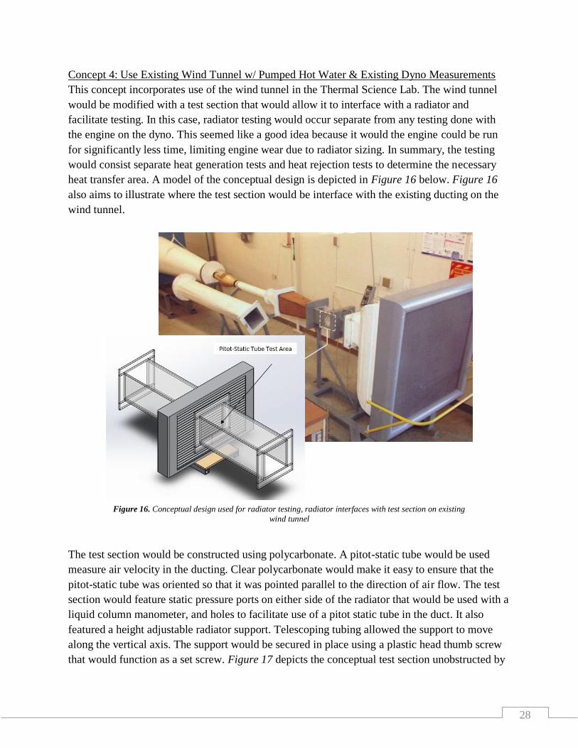
Concept 4: Use Existing Wind Tunnel w/ Pumped Hot Water & Existing Dyno Measurements
This concept incorporates use of the wind tunnel in the Thermal Science Lab. The wind tunnel
would be modified with a test section that would allow it to interface with a radiator and
facilitate testing. In this case, radiator testing would occur separate from any testing done with
the engine on the dyno. This seemed like a good idea because it would the engine could be run
for significantly less time, limiting engine wear due to radiator sizing. In summary, the testing
would consist separate heat generation tests and heat rejection tests to determine the necessary
heat transfer area. A model of the conceptual design is depicted in Figure 16 below. Figure 16
also aims to illustrate where the test section would be interface with the existing ducting on the
wind tunnel.
The test section would be constructed using polycarbonate. A pitot-static tube would be used
measure air velocity in the ducting. Clear polycarbonate would make it easy to ensure that the
pitot-static tube was oriented so that it was pointed parallel to the direction of air flow. The test
section would feature static pressure ports on either side of the radiator that would be used with a
liquid column manometer, and holes to facilitate use of a pitot static tube in the duct. It also
featured a height adjustable radiator support. Telescoping tubing allowed the support to move
along the vertical axis. The support would be secured in place using a plastic head thumb screw
that would function as a set screw. Figure 17 depicts the conceptual test section unobstructed by
Figure 16. Conceptual design used for radiator testing, radiator interfaces with test section on existing
wind tunnel

29
a radiator. Figure 18 aims to depict incorporation of the static pressure ports and adjustable
radiator support. Hoses would be attached to the inlet and exit of the radiator and hot water,
heated with immersion heaters, would be pumped through the radiator.
While the formula team would not have their own wind tunnel to use at the Hangar, there were
many benefits associated with this concept. Constructing the test section would be significantly
less expensive than building an entirely new wind tunnel, and budget became a significant issue
in the other conceptual designs. Additionally, many of the other components necessary would be
readily available in the Thermal Science Lab with the wind tunnel, including: liquid column
manometers, thermocouples, and a pitot-static tubes.
2. Concept Selection
Out of the various concepts listed in the previous section, Concept 4 was chosen. It was
concluded that the benefits associated with time, cost saving, and the guarantee of a working
wind tunnel outweighed the fact that the formula team would not have a wind tunnel to use
simultaneously with the dyno at the hangar. Decision matrices to choose between the 4 concepts
and a QFD to determine which components should be considered with the most care can be
referenced in Appendix B. Heat generated by the engine and heat rejected by the radiator will be
measured separately. In testing heat generation, the engine will be used on the dyno and the
cooling water temperature will be measured at the inlet and exit of the radiator. Equation 14
from Chapter 2, Section 9 will be used to determine heat generation (or heat rejected to the
cooling water) based on mass measured mass flow rate and temperature differential. In testing
heat rejection, hot water will be pumped into the radiator at varying mass flow rates and heat
rejection will be measured over a range of air velocities. In a manner similar to determining heat
generation, heat rejection will be determined by measuring the cooling water temperature at the
inlet and exit of the radiator. The radiator will interface with the test section as illustrated in
Figure 17. Unobstructed view of the test section Figure 18. View of the thumbscrew for height adjustment of
the radiator support and steel tube static pressure ports

30
Figure 16. Any part of the radiator core that is not contained within the ducting will be sealed off
using aluminum foil tape to prevent air leaks.
3. Supporting Preliminary Analysis
Preliminary analysis included the following was performed to determine approximate sizing for
some of the components necessary in the test procedure. This analysis included:
Approximate fan sizing.
Approximate heater sizing.
Consideration of ability of measurement tools to be used.
Fan Sizing
The fan must be sized such that it can pull air through the test radiator at a speed equal to or
greater than the speed at which air would flow the core on the car. It can be observed in Figure 2,
the histogram that describes the number of instances when the car is traveling at a particular
speed, that the maximum speed is 95 ft/s (~65 mph). Testing was performed to determine to the
approximate speed of the air along a streamline as it flows through the radiator. This was
accomplished using a vane type anemometer behind the radiator core. The test process is
described in detail in Chapter 6, Section 1 and the results are outlined in Chapter 6, Section 3.
The maximum necessary velocity in the duct was determined to be 14 m/s. These results were
used to estimate the maximum pressure rise and mass flow rate conditions at which the fan must
be able to operate.
It was determined that the fan must be able to pull air at a mass flow rate of 0.25 kg/s and induce
a pressure rise of about 400 Pa. The fan on the wind tunnel in the Thermal Science Lab is very
nearly capable of achieving this operating point and it can be used to adequately model the on-
car air flow conditions. The calculations used in these estimations are available in Appendix C:
Fan Sizing Program.
Heater Sizing
A calculation was performed to explore the amount of time it would take to heat up different
amounts of water with different combinations of heating power. Affordable heaters available
with McMaster-Carr were rated at 1.15 kW, so the heating power would be some multiple of this
power. A reservoir in the Thermal Science Lab was found that would hold about 17 gallons of
water. It was also determined that the only source of a, for all intents and purposes, limitless
water was available at an initial temperature of 100˚F.
Based on the previously listed values and the fact that it was necessary to heat the water to
180˚F, different multiples of 1.15 kW heaters could be used to predict the amount of time it

31
would take to heat the water with that particular number of heaters. When the 3 heaters were
used, it was predicted that it would take about 57 minutes for the water to heat up. The equations
used in these estimations are available in Appendix D: Heater Sizing Program. Note that in
reality, heating would take slightly longer due to heat loss from the hot water reservoir.
Measurement Instrument Consideration
The static pressure drop across the radiator core will be measured over a range of air velocities.
In order to measure the static pressure drop, a liquid column manometer will be used. There will
be a slight difference in the static air pressure drop measurement when the radiator is being used
to reject heat as compared to when it is cold. This
is due to the change in air density that results
from the increased temperature. A program was
created to determine the pressure change that
would result from the changing air density. The
program was used to determine that an
approximated maximum temperature rise in the
air would be about 18˚C. Then the liquid column
height gradient in the manometer was plotted as a
function of temperature. The plot can be observed
in Figure 19 on the right.
The important idea to recognize in the plot in Figure 19 is that the change in air exit temperature
(in the most severe case) will be responsible for a liquid column height change of no more than
0.003 inches. It would be near impossible to recognize a change in height this small, so it is safe
to assume that the changing air density has no effect on the liquid column manometer reading
which predicts static pressure drop across the radiator. The calculations used in this estimation
are available in Appendix E: Temperature Effects on Manometer Reading Program.
Figure 19. Plot of the effect of exit air temperature on
manometer liquid column height differential

32
Chapter 4: Final Design Description
In order to fulfill the project requirements, this senior project involved both designing
experiments to collect data that would help predict the necessary radiator size, and designing the
equipment necessary to facilitate the experimentation. In the case of this project, a test section
was built that would interface with a radiator and the wind tunnel in the Thermal Science Lab so
that heat transfer experiments could be performed with automotive radiators. The on-car cooling
system conditions would be replicated in the Thermal Science Lab to determine the ability of
different radiators to reject heat. In summary, heat generated in the engine can be predicted as a
function of engine power on the dyno, then the ability of a radiator to reject heat over the entire
operating range of the car can be tested using the test section on the wind tunnel. Using this data,
the necessary size of the radiator can be predicted. This chapter will describe the process by
which the experiments and wind tunnel test section were designed.
1. Overall Description- Testing
The goal of the project was to provide the FSAE team at Cal Poly with a guided process that will
allow the team to perform heat generation and heat rejection testing. Heat rejection testing can be
performed on a wide variety of radiators so that the formula team can determine the radiator
characteristics they determine to be valuable (i.e. fin density, core thickness, manufacturer, etc.)
based on heat rejection achieved. Once they have chosen a type of type of radiator that they
would like to use, they can perform heat generation and heat rejection testing on the dyno and
wind tunnel, respectively to determine how large a radiator they need. The test procedure will be
developed in the following pages of this section. The formula team will be provided with an
Excel program where they can enter data and all pertinent plots will change to reflect the data
they collect. A summary of the tests that must be performed is as follows.
Test 1: Determine mass flow rate of the cooling water as a function of the crank shaft
rotational speed
Test 2: Determine heat rejected from the engine to the cooling water in as a function of
crank shaft rotational speed
Test 3: Determine the mass flow rate of air through the core as a function of car speed
Test 4: Determine static pressure drop in air across the radiator core at different air mass
flow rates
Test 5: Determine heat rejected by radiator as a function of both the mass flow rate of air
through the core and the mass flow rate of cooling water through the radiator
The first three tests were designed so that the formula team could generate curves to predict the
mass flow rates of both air and water through the radiator as well as the heat rejected to the

33
cooling water at each crankshaft rotational speed. This crankshaft rotational speed will correlate
to a specific car speed in each gear. Since the formula team knows the speed at which the car
should be traveling at each point on the FSAE autocross track, they can determine values for
each of the mass flow rates and the heat rejected into the cooling water. The fourth test was
designed for a couple of reasons. First, it was designed to determine the pressure drop across the
radiator at different mass flow rates, to aid the formula team in choosing a cooling fan. Second, it
was used to characterize the mass flow rate of air through the radiator core at different fan speeds
so that the average velocity did not need to be determined with the pitot-static tube each time the
fan speed was adjusted. This way, the mass flow rate of air through the core could be measured
simply using the liquid column manometer. The last test was designed so that the formula team
could generate a curve to predict the heat rejected from the cooling water by the radiator at air
and water mass flow rates that correspond to different car speeds as determined in the first two
tests. Procedural instructions for each of these five tests as well as the process by which they are
used to size the radiator are described in detail in Chapter 6.
2. Detailed Design Description- The Test Section
The design of the radiator test section was governed by design requirements as well as cost
constraints because of the budget uncertainty. The final design of the test section was slightly
different from the one described in Concept Selection (Chapter 3, Section 2) almost entirely due
to budget constraints. It was much more cost efficient to make two major design iterations. First,
the test section would be constructed using sealed and painted plywood instead of polycarbonate.
Second, the height adjustable radiator support would be eliminated in favor of a sawhorse with
pieces of wood stacked to an appropriate height as a free alternative to purchasing the materials
necessary to construct the radiator support. What follows will describe the final design of the test
section used to facilitate the tests described in the previous section. The final design was
governed by the following design requirements.
Section must interface with automotive radiators
Section must interface with the existing ducting on the wind tunnel
Test assembly must be airtight
Section must accommodate static pressure measurement with a liquid column manometer
Section must accommodate use of a pitot-static tube
Radiator Interface
In order to allow radiators to interface with the test section, the test section needed to be designed
so that it is two separate pieces. This way a radiator can be placed between the two pieces of the
test section and air can be directed through the radiator core. Any portion of the radiator core that
is not contained within the test section ducting will be blocked off with aluminum tape so that no

34
forced convection can occur outside of the ducting. Figure
20 aims to illustrate the way a radiator will fit between two
separate pieces of the new test section. The downstream
and upstream pieces of the section will be mounted to the
front and back portions of the wind tunnel, respectively.
The radiator and sawhorse should be placed so that the
radiator fits snug against the downstream piece of the test
section, then the front portion of the wind tunnel can be
pushed back so that the radiator fit snug between the two
pieces of the test section. Closed cell foam would be used
as a gasket material at the interface between each piece of
the test section and the radiator to create an airtight seal.
Wind Tunnel Interface
It was a goal to interface the wind tunnel and the new test section while minimalizing and
alterations to the wind tunnel. As a result, the inside dimensions of the new test section were
made to be 4.8 x 4.8 inches—the same inside dimensions of the ducting on either side of the test
section. The only change that was made to the existing wind tunnel sections had to do with the
brown expansion section that is directly downstream of the original test section. In contrast to the
original test section which is one solid piece, the new test section is two pieces, so each needed
to be supported by the existing sections on either side. The front portion of the wind tunnel can
be pulled away from the rest of the ducting. This front portion originally consisted of the brown
expansion section and each section of ducting that is upstream of it. There was a foam gasket at
the end of the brown expansion section so that it was
airtight when the front portion of the wind tunnel was
pushed up against the back portion. This created an
issue in that section of ducting that comes after the
radiator wouldn’t be connected to anything. To abate
this issue, flanges were added to the wide end of the
brown expansion section and it was connected to the
back portion of the wind tunnel (see Figure 21). The
newly added flange on the brown expansion section
was connected to the flange on the adjacent
downstream duct section using screws and nuts at
each corner of the flanges. In effect, the expansion
became part of the back portion of the wind tunnel
ducting.
Figure 20. The radiator will be secured
between two pieces of the new test section
Figure 21. Method of mounting brown expansion
section to adjacent downstream wind tunnel section

35
Next, the downstream piece of the new test section was
mounted to the brown expansion section in a manner
similar to the one used in mounting the original test section.
Four L-brackets on each side of the square duct were used
to fasten the expansion section to a flange on the new test
section. In effect, the downstream piece of the new test
section also became part of the back portion of the wind
tunnel. Figure 22 depicts the way L-brackets were used to
attach the two sections to one another.
Lastly, the upstream piece of the test section was connected
in the same way the original test section was connected.
Two screw-nut pairs were used to connect a flange on the
upstream piece of the test section to the flange on the
adjacent contraction section on the front portion of the wind
tunnel. In Figure 23 on right, one of the nuts used to
connect the upstream piece of the test section to the existing
wind tunnel section can be observed on the left side flange.
Another screw-nut pair was used in the same manner on the
right side flange.
Airtight Ducting
In order to ensure that the ducting is airtight, strips of closed-cell foam were used around the duct
between each section of ducting. When adjacent sections of ducting are connected, the foam
compresses, creating an airtight seal around the wind tunnel duct. Similarly, foam was used on
the end of each piece of the test section so that the interface between the radiator and each piece
of the test section is airtight when the front and back portions of the wind tunnel are pressed
together with the test radiator between them.
Foam gasket between the radiator and test section Foam gasket between duct sections
Figure 22. Method of mounting downstream
piece of test section to brown expansion section
Figure 23. Method of mounting upstream
piece of test section to adjacent section of the
wind tunnel
Figure 24. SolidWorks model of the test section depicts the use of closed-cell foam gasket material and metal tube location
36
Liquid Column Manometer Accommodation
In order to accommodate the use of a liquid column manometer to determine the static pressure
drop across the radiator core, a metal tube was placed in the bottom of each piece of the test
section downstream and upstream of the radiator core. The metal tubing can be observed on the
bottom of each piece of the test section on either side of the radiator in Figure 24. The barb
fittings on the liquid column manometer are meant to be used with ¼-inch ID tubing. In order to
be sure that there is a good seal between the metal tubing on the test section and the tubing that
goes to the liquid column manometer, the test section was designed so that there was be an
interference fit between the metal and rubber tubing to create a tight seal. To create this
interference fit, 0.259-inch OD metal tubing was used on the test section.
Pitot-Static Tube Accommodation
In order to allow a pitot static tube to be used in the ducting, holes were drilled through the top of
the downstream piece of the test section. These holes are 3/16-inch in diameter—just large
enough so that the elbow of the pitot-static tube can fit through them. The holes were placed as
far downstream as possible to allow as much as distance as possible for the flow to develop once
it passed through the radiator core. These holes can be observed on the downstream piece of the
test section in Figure 22.
3. Cost Analysis
Table 5 in Appendix F details each material that was used for testing throughout the senior
project. A number of materials could be borrowed; those materials have dashes in the cost
columns to indicate that they didn’t cost anything. They are listed in the table to acknowledge
that they were used during testing and may need to purchased in the future if they are no longer
available. The total cost incurred throughout the project was $479.00. The heaters used to heat
the water accounted for almost 50% of the cost of the project. Initially, the plan was to use hot
water from the boiler in the Thermal Science Lab, but the boiler turned out to be unavailable.
This would not have influenced the decision to perform testing by simulating different engine
operating points on the existing wind tunnel in the Thermal Science Lab because this option
would have still more than likely been the most cost effective way and practical way of
performing the testing
4. Geometry, Material, and Component Selection
The geometry of the test section was largely dictated by the fact that it needed to interface with
both the existing wind tunnel sections and a radiator. It is in two separate pieces so that a radiator
could be placed between the two pieces. Then flanges function to interface each section of

37
ducting with the adjacent section. Geometry has been described in greater detail in Detailed
Design Description- The Test Section (Chapter 4, Section 2).
There were four main considerations that needed to be kept in mind in choosing materials and
components to complete the testing. First, it was important to realize that many of these materials
or components would be subject to high temperatures. Second, because of the prevalent use of
water throughout testing, it was also important to realize that there was a possibility of the
components getting wet at one point or another. Third, care needed to be taken to make sure that
every portion of the ducting was airtight. The fourth and last consideration had to do with the
budget. A low cost component was valued more highly than a higher cost component that may
have otherwise been more appropriate in its respective application. The following bulleted points
will list materials and components and describe why they were chosen.
Closed-Cell Foam Gasket Material: The closed-cell foam weather stripping that was used
as a gasket material to maintain an airtight seal between ducting components would come
into direct contact with the hot radiator. Water would enter the radiator at about 180˚F, so
a foam that was rated up to a maximum temperature of 200˚F was chosen.
Rubber Heater Hose: Rubber heater hose was used to plumb the test setup. This hose
would be subject to 180˚F water, and needed to be rated to be able to withstand that high
temperature. The hose used was rated to be used at 212˚F.
Wood: Wood was used to build the test section instead of polycarbonate because it was
significantly less expensive than polycarbonate.
Spackling Compound: When each piece of wood is screwed together, there are still small
gaps between each piece of wood. These gaps would need to be filled using spackling
compound so that the test section would be airtight.
Primer/Sealer: A water-proof primer/sealer needed to be used on the wood because wood
is not particularly resistant to wear due to water.
Hot Water Bath: The Cole-Parmer hot water bath was used because it is was something
that could be borrowed from the Mechanical Engineering department, thus saving money.
It was used solely for its pump and the fact that the pump could withstand high water
temperatures. It would have been much easier to use a pump that could have been
submerged directly into the hot water reservoir, but the opportunity to save money made
the Cole-Parmer hot water bath the best option.
Immersion Heaters: The immersion heaters were chosen because they provided the
highest heating power for the least amount of money. Three 1.15 kW heaters would be
sufficient to heat 17 gallons of water in about an hour and a half.
Sawhorse Radiator Support: The sawhorse was chosen to be used as the radiator support
because it was a zero-cost option that outweighed the benefits of building a radiator
support onto the test section.

38
5. Manufacturing Drawings
See Appendix G for manufacturing drawings and vendor catalog descriptions. Appendix G is
organized so that there is some sort of bill of materials for each system that needed to be
constructed. Vendor catalog pages appear in the order that they are listed in Table 13 with
manufacturing drawings and schematics for those systems that needed to be constructed
preceding catalog pages. Construction instructions for those systems can be found in
Manufacturing Process (Chapter 5, Section 2).
6. Maintenance and Repair Considerations
The wind tunnel and a large majority of the measurement equipment used in testing is property
of Cal Poly and maintained by the Mechanical Engineering department. However, proper care
should be taken so that equipment is in similar or better order than it was before use. The
formula team will only be responsible for maintaining or repairing the test section. Each time the
test section is used on the wind tunnel, the closed cell foam that is being used as gasket material
becomes compressed. If the foam does not return to its original shape, it should be replaced to
maintain an airtight seal. The same goes for the foam used between the test section and the
radiator. If the foam becomes excessively deformed, it should be replaced. Nothing else should
require regular maintenance; however, if something breaks it should be replaced. The
information in Manufacturing Process contains any information the formula team might need to
replace any part that has failed.

39
Chapter 5: Product Realization
The products of this project were the test results and the test section that would need to be
manufactured to facilitate testing. This chapter will describe everything about the process of
manufacturing the test section. Chapter 6 will detail the test procedure as well as the results of
the tests that were performed.
1. Description of Design Iteration
Looking at the finished test section, the most obvious design iteration to the conceptual design is
that it was constructed from ½” plywood instead of polycarbonate. This was a decision that was
made with the budget in mind as the polycarbonate accounted for a significant portion of the
cost. The sheet of plywood that was used for construction was half the price of the polycarbonate
that would have been required. Then, with the same goal of saving money, a decision was made
to eliminate the radiator support from the design. Instead, a sawhorse separate from the test
section was used as a more cost effective alternative. The test section ended up being more of an
extension to the existing wind tunnel ducting that allowed for interface with a radiator and use of
a liquid column manometer and pitot-static tube.
2. Manufacturing Process
The manufacturing process can be broken up into three separate processes. First, the test section
needed to be manufactured to perform Test 4 and Test 5 described in Overall Description-
Testing (Chapter 4, Section 1). Once the test section had been built, it would need to be mounted
on the wind tunnel and then the plumbing would need to be connected. These were the second
and third processes in manufacturing. The following paragraphs will describe these three
processes in detail. Appendix G includes vendor catalog descriptions for all materials referenced.
The Test Section
The test section is in two separate pieces that interface with the wind tunnel on either side of the
radiator. Each duct is composed of twelve individual pieces of wood. The first four pieces are for
the four sides of the duct and the next four are used to construct the flange. Both the duct portion
and the flange constructed are constructed from a ½”- thick sheet of plywood. The last four
pieces of wood were used like brackets in order to ensure that the flanges formed a 90 degree
angle with the duct portion. The manufacturing process will be described in the following
paragraphs.

40
To begin the manufacturing process, the wood was cut using the table saw in the hangar. Table 1
that follows will detail the function of each piece of wood and its dimensions.
Table 1. Description of each piece of wood that would be used in the construction of the test section
Part drawings completed in SolidWorks detail hole locations and dimensioning and can be
observed in Appendix G. A more detailed bill of materials is also included in Appendix G. 1/8”
pilot holes were drilled so that pieces could easily be fastened to one another with #6, 1-1/4”
flathead screws. A table saw was used to cut the wood to size and holes were made with a drill.
With the wood cut, construction would begin by using screws to
fasten wood brackets (Item No. 2) to each piece of the duct (Item
No.’s 1, 3, 4 & 7). These wood brackets were attached so that they
were flush with the edge of the duct. This provided a larger surface
area to attach each piece of the flange and ensure that it formed a
90˚ angle with the duct portion. Figure 25 to the right illustrates
this process with exploded view route lines representing where
screws were used to fasten the bracket to the side of what would
eventually be the duct.
The duct portion was constructed from four pieces of wood similar to
what is shown in Figure 25. The duct sides were sandwiched between
the top and bottom of the upstream and downstream ducting. The
downstream duct top (Item No. 1) differed from the upstream duct top
(Item No. 7) in that it had holes drilled across to accommodate use of a
pitot-static tube in the duct. Figure 26 to the right illustrates the process
by which each side of the duct portion was connected to the adjacent
side. With the completion of this step, the duct portion of the test
section would be finished.
Figure 25. First step: fasten wood brackets to each side of ducting
Figure 26. Second step: construct duct portion

41
The third and final step in the construction process involved
attaching the each piece of the flange to the duct portion that was
constructed in the two previous steps. Once again, the flange was
constructed using four separate pieces of wood: two smaller pieces
and two larger pieces where the smaller pieces were sandwiched
between the large pieces and attached on the end of the duct. The
flanges on the upstream and downstream portions of the test
section differed in that holes were drilled in the upstream large
flange piece (Item No. 5) to mount the test section on the existing
ducting on the wind tunnel. Figure 27 at right illustrates the way
each part of the flange was fastened to the wood brackets. Figure 27 illustrates construction of
the downstream piece of the test section that did not require mounting holes so it could be
mounted with a nut and bolt. Instead, L-brackets would be attached and it would be mounted
with L-brackets onto the brown expansion section as detailed in Detailed Design Description-
The Test Section.
Upon completing the structural construction of each duct,
the spaces between each piece of wood needed to be filled
with spackling compound. For the sake of ease, caulking
was used on the outside of the duct, rather than on the
inside. Once the gaps had been filled caulk in fashion that
was adequate to prevent air leaking from inside the duct,
the test section was sanded, sealed, and painted. At this
point, 1” long, ¼”-OD metal tubing was inserted into the
holes that were drilled to facilitate the static pressure ports,
and the tubing was secured using epoxy. Lastly, weather
stripping was fitted around on either end of the duct to
create an air-tight seal between ducting components and
between the test section and the radiator. Figure 28 on
the left illustrates what the finished test section should look like.
Mounting the Test Section on the Wind Tunnel
As described in Detailed Design Description- The Test Section, the brown expansion section
needed to be modified for the test section to interface with the wind tunnel properly. A flange
needed to be added so that the large end of the expansion section could be attached to the wind
tunnel. A table saw was used to cut the 4 pieces of wood that the flange would be constructed
with: 2 small pieces (7-3/4” x 2-1/8”) and 2 large pieces (12” x 2-1/8”). These were cut from the
same ½” plywood used to build the test section. Then each piece of the flange was glued to the
large end of the brown expansion section using wood glue. To finish the addition of the flange,
the gaps were filled with silicon caulking and 3/8” holes were drilled 10-3/4” from each other at
Figure 27. Third step: attach each part of the flanges
Figure 28. SolidWorks model of the finished test section

42
each corner of the flange. Finally, closed cell foam was fitted around the duct opening on the
flange. Figure 21 depicts the flange that was added to the expansion section.
Before the expansion section was mounted on the wind tunnel, L-brackets were used on each of
the 4 sides of the duct to mount the downstream piece of the test section to the expansion section.
The test section was placed in the proper position on top of the expansion section and the L-
brackets were fastened to each of the two components using the screws that were provided with
the brackets. See Figure 22 to observe the way the L-brackets were attached.
Once the test section was mounted on the expansion section, this assembly could be mounted on
the wind tunnel. 2”-long, ¼” bolts were used with washers and nuts to mount the assembly on
the wind tunnel. Again, this mounting can be observed in Figure 21.
Mounting the upstream piece of the test section on the wind tunnel was much more straight-
forward than mounting the downstream piece. In this case, the holes on the flange of the
upstream piece of the test section were lined up with the holes on the existing contraction section
on the wind tunnel. Then ¼” bolts, washers and nuts were used to mount this piece of the test
section on the wind tunnel in a manner similar to the way the expansion section was mounted on
the wind tunnel. The method for mounting the upstream piece of the test section on the wind
tunnel can be observed in Figure 23.
The Plumbing
Two sets of fittings were needed in the plumbing. First, fittings were needed to accommodate a
component with an embedded thermocouple and two ¾” FPT threads on either side. See Figure
58 and Table 14 in Appendix G to see a list of the fittings needed and a schematic of the way
they should be connected. A valve was also used on the discharge side of the assembly described
above so that the flow of water could be stopped and hot water could be retained in the radiator.
This kept the radiator hot between tests and minimized the time settling time of the water
temperature coming out of the radiator. Teflon tape was used on each set of threads to prevent
leaks between threaded fittings. The length of hose between the radiator discharge and this set of
fittings should be minimized to minimize the potential for heat to escape through the hose. Then
the length of hose between this set of fittings and the valve is not significant. Hose on the
discharge side of the valve should be just long enough to reach a cold water reservoir on the
ground. The length of the hose should always be minimized to minimize head losses.
Then fittings were needed to go from the ¼” FPT threads on the hot water bath pump discharge
to the 1” barb used in the hose. See Figure 59 and Table 15 in Appendix G to see a list of the
fittings needed and a schematic of the way they should be connected. Again Teflon tape was
used on each set of threads. The length of the hose at the discharge of the pump should be just
enough to reach the inlet of the radiator.

43
Chapter 6: Testing
Initially testing was going to be performed to verify the legitimacy of the theoretical process
developed to predict radiator size necessary in achieving adequate cooling. However, the engine
was not available to us throughout the entirety of the senior project. As a result, only testing that
did not require use of the engine could be performed. This meant that three of five tests could be
completed. In the sections in this chapter, the tests will be described (with a list of the necessary
materials and detailed process description) then a detailed discussion of the test results will
follow.
1. Test Descriptions
There are five tests that need to be performed so that the formula team will be able to determine
the size of the radiator necessary in achieving adequate cooling. A summary of the tests that
must be performed is as follows.
Test 1: Determine mass flow rate of the cooling water as a function of the crank shaft
rotational speed
Test 2: Determine heat rejected from the engine to the cooling water in as a function of
crank shaft rotational speed
Test 3: Determine the mass flow rate of air through the core as a function of car speed
Test 4: Determine static pressure drop in air across the radiator core at different air mass
flow rates
Test 5: Determine heat rejected by radiator as a function of both the mass flow rate of air
through the core and the mass flow rate of cooling water through the radiator
The data collected during these tests will be entered into the Excel program that the formula team
will be provided, and any necessary secondary variables or plots will be generated automatically.
Relevant portions of the spreadsheets from the Excel program where collected data will be
entered to determine significant results can be observed in Appendix H. The following pages
describe the test procedures in detail. Data collected can be used to determine the necessary size
of a particular radiator to achieve adequate cooling according to the process described in the
flowchart in Appendix I. The process by which the data can be used to determine the necessary
radiator size will be described following the description of the test procedures.

44
Test 1
The formula team will need to develop a relationship that describes the mass flow rate of the
cooling water as a function of the of the driveshaft’s rate of rotation. With this, the formula team
will be able to predict the mass flow rate of the water at any car speed. In order to develop this
plot, testing will be performed to measure the mass flow rate of the cooling water over a range of
driveshaft rotational rates. The impeller in the water pump is geared to the crankshaft, so the rate
of rotation of the impeller is directly proportional to the rate of rotation of the crank. As a result,
the mass flow rate of the water is dependent on the rotational speed indicated by the tachometer,
and this relationship should not change from gear to gear. This test can be performed with or
without the dyno, but the radiator hoses should not be connected as part of a normally closed
system. The system should be plumbed according to the diagram depicted in Figure 29.
Materials:
Desired Test Radiator
Radiator Hose
Garden Hose
Engine
3 5-Gallon Buckets
Water Source
Stopwatch
Scale
Setup:
Plumb the cooling system so that radiator hose goes from a cold water reservoir (“Bucket 1”) to
the cooling water inlet on the engine, as illustrated in Figure 29 above. The water pump will
draw water in through the cooling canals in the engine block. Plumbing will then travel from the
cooling water exit on the engine though the radiator and to a hot water reservoir bucket (“Bucket
2” or “Bucket 3”). A conscious effort should be made to be sure that the length of the hose used
to plumb the experimental setup is similar to the length of the plumbing on the car. The length of
the hose will affect the flow rate in that the flow rate is a function of the pressure drop in the
system, which is affected by the length of hose used. “Bucket 1” and “Bucket 3” should be
maintained at similar heights so that there is no significant amount of head added to the system,
but it is very important that the water pump does not run dry. Additionally, the water level
relative to the engine should be about equal to that of the on-car condition so that this
gravitational head will not affect the predicted relationship. “Bucket 3” will be used to measure
the weight of the water and determine the mass flow rate.
Radiator Engine
Bucket 1 Bucket 2 Bucket 3
Figure 29. Experimental setup for Test 1

45
Procedure:
1. Weigh the empty “Bucket 3” to determine its weight, in kg.
2. Enter the weight of “Bucket 3” into the Excel spreadsheet.
3. Fill “Bucket 1” with water using a regular garden hose connected to a water spigot.
NOTE: Keep the hose next to the cold water reservoir so that the bucket can be
refilled if the water level becomes too low. Do not let the water pump run dry so as to
avoid cavitation in water pump and overheating in the engine.
4. With the hose coming from the radiator discharge and directing water into “Bucket 2”,
start the engine and allow the water pump to draw water from the cold water reservoir.
Throttle the engine so that it is operating at a continuous driveshaft rotational rate.
5. Once water starts flowing into “Bucket 2,” move the hose from to “Bucket 3” and
simultaneously begin timing with the stopwatch.
6. Allow the water pump to fill “Bucket 3” for 20 seconds.
NOTE: If the bucket fills up too quickly in 20 seconds, test mass flow rate for less
time and change the test time in the Excel spreadsheet.
7. Simultaneously move the hose back to “Bucket 2” and stop the stopwatch.
8. Stop the engine.
9. Weigh “Bucket 3” again to determine its weight with water, in kg.
10. Enter the weight in the Excel program in the cell that corresponds to the driveshaft
rotational rate in the spreadsheet labeled “Cooling Water Mass Flow Rate.”
Analysis:
The Excel program determines the mass flow rate of the water used in the cooling system
according to Equation 1 defined below. Sample data for this test could not be collected
because the engine was never available for testing over the course of the senior project.
However, Figure 30 predicts the general trend that will characterize the relationship.
�� =𝑚𝑤𝑎𝑡𝑒𝑟+𝑏𝑢𝑐𝑘𝑒𝑡−𝑚𝑏𝑢𝑐𝑘𝑒𝑡
𝑡𝑡𝑒𝑠𝑡 (1)
Figure 30. Example of what the plot generated with completion of Test 1 may look like
y = -1E-16x4 + 2E-12x3 - 7E-09x2 + 4E-05x
0
0.05
0.1
0.15
0.2
0.25
0.3
0.35
0 2000 4000 6000 8000 10000Co
olin
g W
ater
Mas
s Fl
ow
Rat
e (k
g/s)
Crankshaft Rotational Speed (RPM)

46
Test 2
In the second test, the formula team will develop a relationship between the heat rejected to the
cooling water in the engine and the rotational speed of the crankshaft. This information will be
used to predict the rate at which heat is rejected to the cooling water at every car speed. To
develop a plot of the heat rejected to the cooling water as a function of the crank speed, the
temperature of the cooling water will be measured as it goes into the engine and travels out of the
engine. This test will be performed on the dyno. The FSAE team’s dyno is already fitted with
thermocouples at the inlet and exit of the engine and the tachometer on the dyno also allows the
rotational speed of the crankshaft to be measured. Details of the test are as follows.
Materials:
Cal Poly FSAE Dyno/Engine Thermocouple Readouts
Setup:
There is minimal setup associated with this test because the dyno is already equipped with
the instruments necessary in gathering the useful data in this test. The engine and cooling
system must be connected on the dyno. Measurements will be taken using the tachometer on
the dyno and the thermocouples at the cooling water inlet and exit on the engine.
Procedure:
1. Start the engine, allowing the cooling water to flow through the radiator.
2. Wait for the engine to get hot.
3. Throttle the engine so it is operating with the crankshaft at a constant rotational speed.
4. Measure the Ti and Te, once these temperatures have reached steady state.
5. Enter the inlet and exit temperatures of the cooling water into the Excel program under
the tab labeled “Heat Generation.”
6. Record the crankshaft rotational rate and repeat this process over a range of crank speeds.
NOTE: The range of crankshaft rotational rates over which the test is performed
should be the same as the range from Test 1.
Thermocouple,
Engine Exit, Te
Tachometer/Scale
Thermocouple,
Engine Inlet, Ti
��
Figure 31. Experimental setup for Test 2

47
Analysis:
The Excel program will use the mass flow rate of the cooling water determined in Test 1, the
specific heat of water and the temperature measurements taken in this test to determine the
heat generated in the cooling water according to Equation 2 that follows.
𝑄 = ��𝑐𝑝(𝑇𝑒 − 𝑇𝑖)
This equation is evaluated where �� is the mass flow rate of the cooling water and 𝑐𝑝 is the
specific heat of water. Again, sample data for this test could not be collected because the
engine was not available for testing over the course of the senior project. The plot depicted
Figure 32 below is an example of what the plot of heat generated in the cooling water over
the range of crank speeds may look like.
The dependent variable is heat generated in the cooling water per unit time, so it is labeled
“Power” on the y-axis. The engine power is plotted on the same graph. Measuring the torque
off the scale on the dyno at each data point to produce the engine power curve is optional.
However, it may be useful to be able to see the engine power and the heat rejected to the
cooling water on the same plot.
(2)
Figure 32. Example of what the plot generated with completion of Test 2 may look like
y = -0.0007x4 - 0.1166x3 + 0.7148x2 + 1.2856x
y = -9E-15x4 + 6E-11x3 + 4E-07x2 + 0.0012x
0.00
5.00
10.00
15.00
20.00
25.00
30.00
35.00
0 2000 4000 6000 8000 10000 12000
Po
wer
(kW
)
Crank Speed (RPM)
Heat Rejected to Water
Engine Power

48
Test 3
A relationship between the car speed and the average velocity (and mass flow rate) of the air
flowing through the radiator core must also be developed. In order to develop this relationship, a
test was performed where a radiator core was held outside the window of a car and a vane type
anemometer was used to take an array of air velocity measurements behind the radiator. Using
this array, an average velocity was determined. The average velocity of the air through the core
can be used with the face area of the radiator core to determine the mass flow rate of the air that
flows through the radiator core. This test was performed while the car was traveling at a range of
speeds from 0-60 mph. Details are as follows.
Materials:
Test Radiator
Car
Vane Anemometer
Setup:
There is no real setup required to perform this test. If the test is performed in the same
manner as it was performed to collect the data for this senior project, three people would be
required to collect data. One person will drive the car, then one person will hold the radiator
outside of the window while another person held the anemometer behind the radiator to
collect data.
Ideally, the test would be performed on the formula car with a fixture to hold the anemometer
behind the radiator in different positions along the face of the radiator to collect an array of
velocity values over a range of car speeds. This is the ideal due to the fact that it is possible
that the relative air velocity is slightly different at different points around the car.
Procedure:
1. The car should be driven at a constant speed.
2. Record the car speed.
3. One person will hold the radiator away from the car while another person holds the
anemometer behind the radiator core.
4. Record data for an array of velocities in different positions over the face of the core.
5. Enter the data into the spreadsheet labeled “Core Air Flow.”
Analysis:
The Excel program will find the average air velocity based on the array of air velocities
measured. Then it will determine the mass flow rate of the air that flows through the core at
each car speed based on Equation 3 below.
��𝑎𝑖𝑟 = 𝜌𝑣𝑎𝑣𝑔𝐴 (3)

49
Equation 3 is evaluated where ρ is the density of air. The density of air assumed to be
constant and equal to its published value of 1.18 kg/m3 at 25˚C. A is the area of the face of
the radiator core. The program will then plot both the average air velocity and the mass flow
rate of the air through the core as a function of the speed of the car. The Excel program was
used to develop this plot for sample data collected that was collected. The results are depicted
in Figure 33 below.
Both the average air velocity and the mass flow rate of the air through the core are plotted on
the graph using the Excel program. It will be helpful to know both the average air velocity
and the mass flow rate of the air through the core to correlate data points in the results of Test
4 and Test 5 to actual car speeds. Results from the test will be discussed in depth in the Test
Results (Chapter6, Section 3).
Figure 33. Plot of results from completion of Test 3
y = 0.0182x
y = 0.5315x
0
2
4
6
8
10
12
14
16
0 5 10 15 20 25 30
0.0
0.1
0.2
0.3
0.4
0.5
0.6
Ave
rage
Air
Vel
oci
ty (
m/s
)
Car Speed (m/s)
Air
Mas
s Fl
ow
Rat
e (k
g/s)
Air Mass Flow Rate
Average Air Velocity

50
Test 4
This test is the first of two tests to be performed on the wind tunnel in the Thermal Science Lab.
A relationship between the average air velocity through the radiator core and the static pressure
drop across the core will be established. This relationship will be used in two ways: first it will
be helpful in measuring the mass flow rate of air through the core in Test 5, and second it will be
helpful in choosing a fan to be used on the formula car. In order to develop this relationship, the
radiator to be tested will be mounted in the test section, then a pitot-static tube will be used to
determine the velocity of the air over an array of positions on the face of the radiator core. A
liquid column manometer will be used to determine the pressure drop across the radiator. The
details of this test will be described in the next few paragraphs.
Materials:
Wind Tunnel w/ Test Section
Aluminum Foil Tape
Test Radiator
Saw Horse
Inclined Liquid Column Manometer
¼” ID Flexible Plastic Tubing
Pitot-Static Tube w/ Readout
Square Ruler
Setup:
To prepare for data collection in Test 4, the radiator core needs to be covered with aluminum
foil tape on both sides where it will not be contained within the wind tunnel ducting, as
depicted in Figure 34. This to ensure that the core is airtight; air should only pass through the
fins contained within the wind tunnel ducting. The face area tested will be used to predict the
necessary face area of the radiator core to achieve adequate cooling on the formula car. If
more fins are rejecting heat, the face area reference used in these tests will be meaningless
and the necessary face area predicted will be wrong. Additionally, the aluminum foil tape
Figure 34. Experimental setup for Test 4-
ensuring the core is airtight
Figure 35. Experimental setup for Test 4- securing the radiator
between the two test section pieces

51
should not cover any part of the core that is contained within the ducting. Once the face area
outside of the duct has been covered with aluminum foil so no air can escape the core, the
radiator can be mounted in the test section, as depicted in Figure 35. The front end of the
wind tunnel where air enters is on wheels while the back with the fan is stationary. The saw
horse should be positioned so that it will be underneath the radiator when the front end of the
wind tunnel has been pushed against the radiator. If the saw horse is too short, boxes or other
materials can be used on top of the sawhorse to support the radiator in the test section. It can
be observed in Figure 35 that a box was used on top of the sawhorse to support the radiator
in the proper vertical position. Once the proper vertical position is achieved, the front end of
the wind tunnel can be pushed against the radiator core. Check around the foam gasket to be
sure that no fins are visible.
Lastly, use two pieces of rubber tubing to connect the static pressure ports on the test section
to the inclined liquid column manometer mounted on the wall behind the wind tunnel.
Connect one end of the tubing to the test section as
depicted in Figure 36 to the right. The other end of
the tubing will be connected to the barb fitting on top
of the liquid column manometer. The tubing should be
placed such that the static pressure port in front of the
radiator is connected to the barb fitting on the left side
of the manometer. The static pressure port behind the
radiator will be connected to the barb fitting on the
right side of the manometer. As a result, the higher
pressure that exists in front of the radiator will push
the height of the inclined liquid column down with
resistance from the lower pressure on the other side of
the column.
Procedure:
1. Move the lever on the circuit breaker for the wind tunnel (located behind the wind tunnel)
to the “On” position.
2. Set the fan to a low speed using the variable frequency drive (VFD, located on the wind
tunnel near the test section).
3. Flip the switch on right on the VFD to the “Start” position.
4. Insert the pitot-static tube into one of the holes on top of the test section and pull up so
that the tip of the pitot-static tube is at the top of the duct. This will measure the velocity
of the incoming/outgoing air at that point on the face. Use a square ruler to be sure the
pitot-static tube is straight up and down and the tip is pointed directly towards the
incoming air flow (See Figure 37).
Figure 36. Experimental setup for Test 4-
connecting the tubing to the static pressure ports on the test section

52
5. Record the velocity measurement in the Excel program using the spreadsheet labeled
“Core Pressure Drop.”
6. Use the ruler to move the pitot-static tube down 1-1/8 inches and measure the velocity at
that point on the radiator face and record the measurement in the Excel program.
7. Repeat Step 6 until 5 measurements have been
taken in that hole.
8. Repeat Step 4 through Step 7 until
measurements have been taken in each of the
5 holes along the top of the test section.
9. Observe the difference in the difference in
height of the two oil columns in the inclined
liquid column manometer on the wall and
record the value in the Excel program.
10. Repeat Step 4 through Step 9 over a range of
fan speed settings.
Analysis:
The Excel program will use the values from each array of measurements to determine the
average velocity of the air that passes through the core. From this average velocity, the mass
flow rate of the air in the duct can be determined in the same way it was determined in Test 3
using Equation 3. It will then plot both the velocity of the air in the duct and the mass flow
rate of the air in the duct as a function of the pressure drop reflected by the change in height
of the liquid column manometer. The first plot generated by the Excel program with results
from testing performed can be observed in Figure 38 below.
This plot can be used as a calibration curve to determine the average velocity of the flow in
the duct. This will be valuable in Test 5, so that mass flow rate at any fan speed can be
determined using the liquid column manometer.
Figure 37. Orientation of the pitot-static tube in the
test section during Test 4
y = 10.214x0.6294
y = 0.1793x0.6294
0.00
0.05
0.10
0.15
0.20
0.25
0
2
4
6
8
10
12
14
0 0.2 0.4 0.6 0.8 1 1.2 1.4 1.6
Air
Mas
s Fl
ow
Rat
e (k
g/s)
Ave
rage
Vel
oci
ty (
m/s
)
Static Pressure Drop (inOIL)
Average Velocity
Air Mass Flow Rate
Figure 38. Plot of results from Test 3- average air velocity and mass flow rate associated with static pressure drop

53
The spreadsheet for this test will produce another plot. This plot develops a relationship
between the mass flow rate of the air through the core and the static pressure drop associated
with it for the radiator core as a loss element. This information will be valuable in selecting a
fan if the formula team determines a fan is necessary to keep the engine cool. The second
plot generated using the Excel program with results from testing performed can be observed
in Figure 39 below.
y = 3799.8x2 + 446.02x
0.00
50.00
100.00
150.00
200.00
250.00
300.00
350.00
0.0000 0.0500 0.1000 0.1500 0.2000 0.2500
Stat
ic P
ress
ure
Dro
p (
Pa)
Mass Flow Rate of Air Through Core (kg/s)
Figure 39. Plot of results from Test 3- static pressure associated with mass flow rate of air through the core

54
Test 5
This test is the second of the two tests that are performed on the wind tunnel in the Thermal
Science Lab. A relationship between the flow rates of air and water and the heat rejected by the
radiator will be established. In order to develop this relationship, the radiator to be tested will be
mounted in the test section, then thermocouples will be used to measure the temperature of the
water at the inlet and outlet of the radiator. The temperature drop across the radiator can be used
to find the heat rejected by the radiator over a range of mass flow rates of both air and water.
This data will generate a curve that will allow the formula team to predict the heat rejected by
their radiator per unit area over the car’s operating range. Details are as follows.
Materials:
Plumbing Assemblies from Appendix G
Cole Parmer Hot Water Bath
¼” Brass Pipe Plug Fitting
2-Quart Pot w/ Handle
Aluminum Foil Tape
20-Gallon Reservoir
Immersion Heaters
2 Extension Cords
2 Surge Strips
Test Radiator
Inclined Liquid Column Manometer
¼” ID Flexible Plastic Tubing
Wind Tunnel w/ Test Section
Type K Thermocouple Wire
2 Thermocouple Readouts
Thermocouple Jack
2 5-Gallon Buckets
Stopwatch
Sawhorse
Stir Stick
Setup:
Setup should begin almost exactly as Test 4 was set up. The test radiator needs to be covered
with aluminum foil so that no air will escape the test section and the covered radiator needs to be
secured between the two pieces of the test section on a sawhorse. Then two lengths of flexible
plastic tubing need to be attached between the static pressure port tube on bottom of the test
section and the barb fittings on the liquid column manometer. Again, this tubing should be
attached so that the tubing attached to the upstream piece of the test section goes to the barb
fitting on the left side of the liquid column manometer near the 0” designation. The tubing
attached to the downstream piece of the test section will go to the barb on the right side of the
liquid column manometer. Place the hot water bath in the spot where it will stay during testing.
Next the plumbing needs to be set up. Begin by using the brass pipe plug described in Appendix
G to plug the hot water bath’s pump suction. Next, construct the pump discharge assembly
described in the Figure 59 and Table 15, in Appendix G. Apply Teflon tape to all external
threads. The ¼” MPT nipple on this assembly should be threaded into the hot water bath
discharge on the right side of the back of the hot water bath. At this point, the heater hose can be
fitted on the barb at the other end of the pump discharge assembly. Use a hose clamp to secure

55
the hose on the barb. The other end of the heater hose should be cut so that it just reaches the
radiator inlet. Place the hose over the radiator inlet and use a clamp to secure the hose around the
inlet. Similarly, construct the thermocouple assembly described in Figure 58 and Table 14, in
Appendix G; again, using Teflon tape on all male threads. Cut a 3” long piece of heater hose and
use clamps to attach one end to the radiator outlet and the other end to a barb on the
thermocouple assembly. Cut another piece of heater hose about 6” long. Attach one end of the
hose to the other end of the thermocouple assembly and the other end to one end of the valve.
Use clamps to secure each end of the hose. Cut another piece of heater hose that is just long
enough to go from the other end of the valve to the furthest of two discharge water reservoir
buckets on the ground. Use a clamp to attach one end of the heater hose to the discharge end of
the valve.
Plug the banana plugs from the embedded thermocouple into the thermocouple jack and then
plug the wire from the jack into a thermocouple readout. Similarly, plug the thermocouple wire
into the other thermocouple readout. The thermocouple wire can be placed inside the red hole on
the back right corner of the hot water bath. Figure 40 below depicts the way the test should be
set up.
The valve at the radiator outlet, and the pump discharge assembly are not visible in the figure
above, but should absolutely be implemented. The thermocouple wire that is used to measure the
inlet water temperature in the hot water bath can be placed in the red hole at the back right corner
of the hot water bath as described above. Again the figure above does not depict this
implementation.
Figure 40. Experimental setup for Test 5
Thermocouple
Assembly
Pump Discharge
Assembly (Not
Shown)
Thermocouple
Jack
Thermocouple
Readout, Outlet
Discharge Water
Reservoir Buckets
Thermocouple
Wire, Inlet
(Readout Not
Shown)
Hot Water
Bath (Controls)
Valve should go here,
reference Figure 60

56
Procedure (Heating the Water):
1. Begin by filling the 20-gallon reservoir with about 17 gallons of water. The hotter the
water begins, the faster the water will heat up to the appropriate temperature, so a water
source with the hotter water should be used.
2. Place the immersion heaters in the reservoir.
NOTE: Do not allow the bottom of the black plastic at
the top of the heater dip below the water level.
3. Plug the extension cords into the wall and the surge strips
into the extension cords. Then plug the immersion heaters
into the surge strips. Turn the surge strips on.
NOTE: Plug no more than two heaters into one of the
surge strips.
4. Allow the water to heat up to 180˚F (or whatever the target
temperature for the cooling fluid flowing into the radiator
is determined to be). Stir the water every 10 minutes because the water will stratify and
take excessively long to reach the target temperature. While the water is heating up,
continue with the procedures below.
Procedure (Measuring Water Flow Rates):
1. Weigh one of the buckets being used at the radiator outlet to determine its weight, in kg.
2. Enter the weight of the bucket into the Excel spreadsheet titled “Heat Rej. from Rad.”
3. Fill the hot water bath with tap water.
4. Move the outlet hose to the bucket that was not weighed.
5. Be sure that the valve at the radiator outlet is open and turn the hot water bath pump on
using the power button on the control panel.
NOTE: The hot water bath is only being used for its pump, it is not being used to heat
up water at any time.
6. Adjust the pump speed by pressing down on the knob until you have reached pump speed
selection and turn the knob to select the pump speed. When the desired pump speed is
selected, press the knob down again.
7. Turn the pump off.
8. Refill the hot water bath, if necessary.
9. Turn the pump back on and allow water to flow into the bucket.
10. Move the hose into the bucket that was weighed and simultaneously begin timing with
the stopwatch.
11. Allow the pump to fill the bucket for 20 seconds.
12. At the end of the 20 seconds move the outlet hose back to the other bucket.
13. Turn the pump off.
14. Weigh the bucket again to determine its weigh with water, in kg.
15. Enter the weight into the Excel spreadsheet to produce water mass flow rate.
Figure 41. Heating water using immersion heaters

57
16. Repeat this process to determine mass flow rates at 4 pump speeds (slow, medium, fast,
and maximum).
Procedure (Measuring Air Mass Flow Rates):
1. Make 5 marks with pencil on the variable frequency drive on the wind tunnel. These will
be the air speeds at which testing is performed.
2. At each of these 5 speeds, record the pressure drop across the radiator, in inches of oil.
3. Record these values in each of the 4 tables in the Excel spreadsheet.
4. Change the equation in the “Air Mass Flow Rate” column to correspond to the
relationship between air mass flow rate and static pressure drop (in inches of oil) to
produce air mass flow rates specific to the system setup at each of the 5 speeds.
Procedure (Measuring Heat Rejection):
1. Use the pot to transfer hot water into from the hot water reservoir into the hot water bath.
2. Be sure that the valve at the radiator outlet is open and the end of the heater hose is in a
bucket. Turn the pump on and allow it to run until water begins to flow into the bucket.
3. Turn the pump off and close the valve to allow the hot water trapped in the radiator to
heat up the radiator.
4. Wait about 5 minutes then begin testing by opening the valve and allowing the water that
was trapped in the radiator to flow out. This will heat up the radiator.
5. Set the fan to one of the predetermined speeds then simultaneously turn the fan and the
pump on.
6. Watch the thermocouple readout at the radiator outlet. Once, the outlet temperature has
reached steady state, record the inlet and outlet water temperatures.
7. Change the fan and pump speeds and repeat this process 19 times for each combination
of fan and pump speeds.
8. Enter the inlet and outlet water temperatures into the appropriate cells in the Excel
spreadsheet to determine the relationship between fluid mass flow rates and heat rejected
from the radiator.
Analysis:
The Excel program will use the inlet and outlet water temperature values and the mass flow rate
of the water to determine the heat rejected from the water via the radiator. This heat can be
predicted using to the aforementioned inputs via Equation 4 below.
𝑄 = ��𝑐𝑝(𝑇𝑜 − 𝑇𝑖)
Where the outlet and inlet temperatures are 𝑇𝑜 and 𝑇𝑖, respectively. Then �� is the mass flow rate
of the water and 𝑐𝑝 is the specific heat of the water at an average temperature.
(4)

58
The Excel spreadsheet will then produce two different plots. It will produce two plots where heat
rejection rate, in kW, is plotted on the y-axis with two independent variables. The first plot has 5
different graphs with water mass flow rate on the x-axis. Each of the 5 graphs correspond to a
different air mass flow rate. Figure 42 contains a plot generated with real test data.
The next plot is very similar to the first plot, except in this case, there are 4 different graphs with
air mass flow rate on the x-axis. Each of the 4 graphs correspond to a different water mass flow
rate. Another plot generated with real test data can be observed in Figure 43 below.
Predictably, the rate at which heat is rejected from the radiator increases as the mass flow rates of
either of the fluids increases. The data indicates that the heat rejection increases at a decreasing
rate as the mass flow rate of air increases. Conversely, the data suggests that the heat rejection
rate increases linearly as the mass flow rate of water increases.
y = -90.703x2 + 31.351x + 0.3703y = -134.38x2 + 40.983x + 0.3816
y = -152.24x2 + 46.935x + 0.3382
y = -73.63x2 + 37.149x + 0.7778
0
1
2
3
4
5
6
0.00 0.02 0.04 0.06 0.08 0.10 0.12 0.14 0.16 0.18 0.20
Hea
t R
ejec
tio
n R
ate
(kW
)
Air Mass Flow Rate (kg/s)
H2O = 0.168 kg/s
H2O = 0.207 kg/s
H2O = 0.230 kg/s
H2O = 0.322 kg/s
Figure 42. Heat rejection rate as a function of water and air mass flow rates- water mass flow rate on the x-axis
Figure 43. Heat rejection rate as a function of water and air mass flow rates- air mass flow rate on the x-axis
y = 4.5693x + 0.575
y = 3.1664x + 1.8439
y = 8.0678x + 1.4878
y = 9.9728x + 1.2466
y = 12.516x + 1.0104
0
1
2
3
4
5
6
0 0.05 0.1 0.15 0.2 0.25 0.3 0.35
Hea
t R
ejec
tio
n R
ate
(kW
)
Water Mass Flow Rate (kg/s)
Air = 0.0336 kg/s
Air = 0.0671 kg/s
Air = 0.0991 kg/s
Air = 0.1367 kg/s
Air = 0.1748 kg/s

59
Using Experimental Results to Size the Radiator
The flowchart in Appendix I will walk the user through the process of using the experimental
results to size the radiator. To begin, the user must select a type of radiator that they want to use.
This type of radiator should be characterized by its fin density, its depth, and the material that it
is made from. Then the user must select a “worst-case scenario” that they would like to use as a
design point. This “worst-case scenario” is the operating point that results in a high rate of heat
rejection from the engine to the cooling fluid and a low rate of heat rejection from the cooling
fluid to the air via the radiator. This will most likely come in low gears (i.e. first gear) at high
engine outputs. At this point, the car will not be going very fast, so the mass flow rate of air
through the core is low, resulting in a low rate of heat rejection from the cooling fluid to the air.
There is still a maximum engine output in first gear around 8500 RPM, so if the car will ever
operate in first gear at 8500 RPM, this may be the worst case scenario. The formula team will
need to determine on their own whether or not this is truly the worst case scenario that they will
use as a design point. If the cooling water flow rate changes significantly as the crank speed
increases, this may not be the worst case scenario because the water flow rate is so high.
Determination of the “worst case scenario” will necessitate some exploration. For the purpose of
describing the process of sizing the radiator, the max engine output in first gear will be treated as
the design point.
The formula team will use the equations of the curves generated by the plot from Test 1 (Figure
32) and the plot from Test 2 (Figure 32) to determine the mass flow rate of the cooling water and
the rate at which heat is rejected to the cooling water, respectively, at the design point. They will
also use the gear ratio and the radius of the tire to determine the speed of the car at this point.
The speed of the car will can be determined according to Equation 5 below
𝑣 = (𝑁𝑒 ∗2𝜋
60)
1
𝜉𝑡𝜉𝑎𝑟𝑤
where v is the velocity of the car, Ne is the rate of revolution of the crankshaft (RPM), ξt and ξa
are the gear ratios for the transmission reduction and the drive axle, respectively, and rw is the
radius of the tire.
Once the formula team has determined the speed of the car at the design point, they will use
equation of the curve generated by the plot from Test 3 (Figure 33) to determine the mass flow
rate of air through the core at the design point. This mass flow rate of air and the determined
mass flow rate of water will be used with either of the plots from Test 5 to determine the rate at
which heat will be rejected from the cooling water via the radiator. The heat rejection rate
measured in Test 5 can be viewed as the heat rejection rate per heat transfer area (or the surface
area of the fins contained within the duct during testing). To determine the surface area necessary
to achieve adequate cooling, simply divide the rate at which heat is rejected from the engine to
(5)

60
the water by the rate of heat rejection from the water to the air per unit area, according to
Equation 6 as follows.
𝐴𝑟𝑒𝑞 = 𝐴ℎ𝑡 ∗𝑄2
𝑄5
In the above equation, Areq is the required heat transfer area (the surface area associated with the
sum of the fins in the core), Aht is the heat transfer area as previously described—the surface area
of the fins contained within the duct during testing, then Q2 and Q5 are the heat rejection rates
determined in Test 2 and Test 5, respectively.
If the necessary radiator size determined is acceptable, then the radiator sizing is completed;
however, it could be beneficial to use a fan to increase the mass flow rate of air at your design
point, thus lowering the necessary heat transfer area. If this is the case, the user should continue
as the flowchart suggests. They will choose an area where they believe this would be beneficial
and use the results from Test 5 to determine the mass flow rate of air associated with adequate
cooling using the heat transfer area that has been chosen. They will then use the results from Test
4 (Figure 39) to determine the static pressure drop associated with the new and old air mass flow
rates. Then a fan must be chosen that can supply the difference in the static pressure drop at the
mass flow rate chosen.
The formula team may also decide that a fan is necessary because the worst case scenario is
when the car is idling. If this is the case, the process above should be performed where the design
point are the conditions at idle. The mass flow rate of air through the core is zero when the car is
idling, so a fan will be necessary. They would need to choose a fan and radiator size combination
that would satisfy the cooling requirements as described above.
(6)

61
2. Safety Considerations
This section contains a discussion regarding safety considerations that should be made
throughout the testing process. It describes the consequences of failing to use proper care during
testing as well as the severity if that consideration is not heeded, and methods of avoiding
potentially dangerous situations.
1. The valve at the outlet of the radiator needs to be opened before the pump is turned on.
Consequences: The clamps could fail and water could be sprayed on the user. The user
could be burnt by hot water or slip in a puddle.
Severity: Severe
Solution: The user should always be sure the valve is open before the pump is turned on.
2. Any material making contact with the radiator in testing should be resistant to burning.
Consequences: The radiator will be hot, if plastic is used to as a support, it could burn,
resulting in potentially toxic fumes.
Severity: Moderately severe
Solution: Only burn-resistant materials (i.e. wood, 180˚ rated foam) should come in
contact with the radiator.
3. Do not touch the radiator, hoses, hot water, hot water reservoir, or engine during testing as
they will all be very hot.
Consequences: The user runs the risk of being burnt by hot materials.
Severity: Severe to very severe
Solution: Care should be taken during testing to be sure that the user does not come into
contact with any of the aforementioned objects. Wear pants, long sleeves, and gloves
when necessary.
4. The plumbing should not leak.
Consequences: The user runs the risk of being burnt by hot water that drips from
plumbing and slipping in a puddle of water that has gone unnoticed.
Severity: Moderately severe to severe
Solution: The user should be aware of their surroundings and check the plumbing before
each test to be sure that hot water is not leaking.
5. Water should not be spilled when it is being transferred.
Consequences: If water is spilled, the user may be burnt by hot water, or slip in the
resulting puddle.
Severity: Moderately severe to severe
Solution: The user should exercise care when transferring water.

62
6. Any buckets used as reservoirs should not be allowed to overflow.
Consequences: If water spills, the user runs the risk of slipping in the resulting puddle. If
hot water is spilled, the user could be burnt.
Severity: Moderately sever to severe
Solution: The user needs to pay special attention to be sure that the buckets never
overflow.
7. When performing Test 3, the users should exercise caution throughout the entire test.
Consequences: The driver could become distracted and hit something. If the user holding
the radiator drops it, it could hit another user.
Severity: Moderately severe to very severe
Solution: The driver needs to always pay attention to the road and other users should
firmly grasp any object being held outside of a moving car.
8. The immersion heaters should not be allowed to short circuit.
Consequences: If the heaters short circuit, the heaters could be damaged or the user could
be electrocuted.
Severity: Very severe
Solution: The user should always be careful to keep any surge strips outlets well out of
the way of water.
9. The radiator should be properly supported from below.
Consequences: The radiator could fall from between the two pieces of the test section. If
the radiator falls, it is possible that they plumbing detaches from adjacent components,
resulting in hot water being spilt and the potential for users to be burnt. The radiator may
be damaged as well.
Severity: Very severe
Solution: The radiator support should be stable.
3. Test Results
This section will discuss the results of the sample testing that was performed. As a result of the
fact that the engine was unavailable for testing, the first two tests could not be performed.
However, sample data was acquired for the last three tests. The results that would have been
expected from Test 1 and Test 2 as well as the results from the last three tests will be detailed.

63
Test 1
In Test 1, the relationship between the rate of rotation of the crankshaft and the mass flow rate of
the cooling fluid (which, in this case will be water) is established. This test is performed so that
the formula team will be able to predict the mass flow rate of the water, which will be dependent
on the power delivered to the system by the pump’s impeller. Since the impeller is connected to
the crankshaft and power delivered to the crankshaft will increase from idle until the engine’s
maximum power output at about 8500 RPM, the mass flow rate of the water should increase
from idle to 8500 RPM, then begin to dip back down at higher crank speeds. Results should be
characterized by a plot similar to the one shown below in Figure 44.
Figure 44. Predicted relationship between cooling fluid mass flow rate and crank speed from Excel program
Test 2
In Test 2, the relationship between the rate of rotation of the crankshaft and the rate at which heat
is rejected from the engine to the cooling water is established. Theoretically, about 30% of the
engines rated power is rejected to the cooling water in the form of heat. This theory establishes a
proportional relationship between the engine’s output power and the rate at which heat is rejected
to the cooling water. As a result, the trend that predicts the rate at which heat is rejected to the
cooling fluid should be similar to the plot of the results from Test 1. Results should be
characterized by a plot similar to the one shown below in Figure 44.
Both the engine power and the rate at which heat is rejected to the cooling fluid as a function of
crankshaft rotational speed are plotted in the Excel program. It is not necessary to collect data to
plot engine power, but it may be interesting to test the theory that predicts that 30% of the
engines rated power is rejected to the cooling water in the form of heat. Theoretically predicted
results are plotted in Figure 45 that follows.
y = -1E-16x4 + 2E-12x3 - 7E-09x2 + 4E-05x0
0.05
0.1
0.15
0.2
0.25
0.3
0.35
0 2000 4000 6000 8000 10000
Co
olin
g W
ater
Mas
s Fl
ow
Rat
e (k
g/s)
Crankshaft Rotational Speed (RPM)

64
Figure 45. Predicted relationship between rate of heat rejection to the cooling fluid and crank speed from Excel program
Test 3
From this point on, sample data was collected. In Test 3, the relationship between car speed and
the mass flow rate of air through the radiator core was predicted. As described in Test
Descriptions, the velocity of air was measured at different points along the face of a radiator that
was being held out of window. This data yielded an average velocity of air through the core,
from which the mass flow rate of air through the core could be determined. The raw data results
are can be observed in the tables below.
y = -0.0007x4 - 0.1166x3 + 0.7148x2 + 1.2856x
y = -9E-15x4 + 6E-11x3 + 4E-07x2 + 0.0012x
0.00
5.00
10.00
15.00
20.00
25.00
30.00
35.00
0 2000 4000 6000 8000 10000 12000
Po
wer
(kW
)
Crank Speed (RPM)
Heat Rejected to Water
Engine Power
Table 4. Array of measurements of air velocity through core, car speed = 50mph
Table 3. Array of measurements of air velocity through core, car speed = 30mph
Table 2. Array of measurements of air velocity through
core, car speed = 20mph
Table 5. Array of measurements of air velocity through
core, car speed = 40mph
Table 6. Array of measurements of air velocity through
core, car speed = 60mph

65
Contrary to what was expected, there was not a major difference in the velocity along the edges
of the radiator core. In the case of the radiator that was tested, the average velocity of air through
the radiator core could have almost been predicted by measuring the velocity at an arbitrary point
along the face because there was such insignificant variance.
The data from the tables was used to generate the plot in Figure 46 below. This plot displays the
relationship between car speed, the average velocity through the radiator core and the mass flow
rate of air that results.
Since the density of the air is constant along at each car speed, the mass flow rate and average
velocity of air through the radiator core are directly proportional. The trendlines on the plot are
not perfectly parallel because they are plotted on different scales. The plot suggests that the
relationship between the speed of the car and the average velocity (and thus the mass flow rate)
of air through the core is quite linear. The measurements beyond 15 mph suggest that the
relationship is almost perfectly linear. This is most likely due to measurement error and the effect
of wind being more significant at lower speeds. This seems to be the most likely cause of the
drop in average velocity through the core at low speeds because when the trendline is forced
through the origin, the resulting trendline almost perfectly intersects every point at speeds above
15 mph. The trendline should intersect the origin because the velocity of air through the car
should be zero when the car is idle. However, the accuracy of the trendline is appropriate in these
circumstances and it can be assumed that there is a linear relationship between the velocity of air
through the core and the car speed. In other words, as the speed of the car increases, the velocity
of the air that passes through the radiator increases proportionally.
y = 0.0182x
y = 0.5315x
0
2
4
6
8
10
12
14
16
0 5 10 15 20 25 30
0.0
0.1
0.2
0.3
0.4
0.5
0.6
Ave
rage
Air
Vel
oci
ty t
hro
ugh
Co
re
(m/s
)
Car Speed (m/s)
Mas
s Fl
ow
Rat
e o
f A
ir t
hro
ugh
Co
re
(kg/
s)
Air Mass Flow Rate
Average Air Velocity
Figure 46. Measured relationship between the average air velocity and mass flow rate of air through the core
and car speed

66
Test 4
In Test 4, the relationship between the mass flow rate of air through the core and the static
pressure drop across the core was established. This was useful for a few reasons. First, it made it
so that the average velocity of air in the duct could be predicted using the static pressure drop
indicated by the liquid column manometer any time the fan speed was changed. Second, it aided
in choosing a fan. This way, the formula team would know the back pressure associated with a
mass flow rate of air through the radiator. They can choose a fan based that can generate enough
head to overcome the pressure drop across the radiator at their desired mass flow rate. As
described in Test Descriptions, the average velocity of air through the core was predicted using a
pitot-static tube to find the air speed at 25 different points along the face of the radiator. These 25
points made for a nice average that would negate the effects of any human error during testing.
This test was performed for two different radiators. The first
radiator was a radiator provided by the formula team that was
a downflow radiator with a 1” thick core. The second radiator
was a C&R racing radiator. It was a crossflow radiator with a
1.35” thick core with a higher fin density. Figure 47 on the
right depicts the radiator that was borrowed from the formula
team for testing. Figure 48 and Figure 49 depict the two sides
of the C&R racing radiator core. The radiator received from
the formula team has a significantly lower fin density as
compared to that of the C&R core. Notice that one can see
straight through the fins on this radiator, while this is not the
case for the C&R core.
Figure 49. C&R racing radiator, undamaged fins
Figure 48. C&R racing radiator, notice
damaged fins in the top right hand corner of the
exposed area
Figure 47. Core of radiator borrowed from
the formula team

67
Test 4 was performed on both radiators. The tables below contain raw data collected during the
experiment. The test was performed at 9 different air speeds in the case of the formula team’s
radiator and 6 different speeds in the case of Professor Fabijanic’s radiator. The trends were
relatively similar over the range of airspeeds for each respective radiator.
Table 7 indicates that there is some disparity between the velocity readings taken in the middle
of the duct and those taken at the corners of the duct. This is to be expected as a result of the
formation of a boundary layer inside the ducting. The velocity should be at a maximum in the
center of the duct and then eventually go to zero at a point infinitely close to the duct wall. The
evidence of a boundary layer was not significant at middle positions along the edges, but was
very apparent at the corner positions.
Table 8 contains raw data taken from testing on the thicker racing radiator. At every velocity,
there was a region in the top left portion of the ducting where the air velocity was zero. This was
due to what seemed to be relatively minor damage to the fins (see Figure 49). This relatively
minor fin damage proved to be very significant. It wouldn’t be as significant in the case of heat
rejection on the wind tunnel as it would be on the car. On the wind tunnel, the same mass flow
rate of air will be forced through a smaller area. There would only be a small dip in the mass
flow rate of air due to the increased system back pressure. The most significant cause of reduced
heat rejection would be due to the fact that there are fins that are not being used to reject heat,
not the slightly reduced mass flow rate of air through the core. However, on the car, it will be as
Table 7. Array of air velocity measurements behind the radiator in the wind
tunnel ducting, formula team's radiator core
Table 8. Array of air velocity measurements behind the radiator in the wind
tunnel ducting, C&R racing radiator core

68
though that entire area didn’t exist. Not only would those fins not reject heat, but a large portion
of the air that would have gone through that area would just go around the radiator.
The data collected was used to produce two different plots for each radiator. One plotted the
mass flow rate and the average velocity of the air through the radiator core against the difference
in height of the liquid columns on the inclined manometer. This plot was used mainly as a
calibration curve to predict the average velocity and mass flow rate of air through the duct at
different fan speeds based on the manometer measurement. These calibration plots can be
observed in Figure 50 and Figure 51 below. The liquid column manometers measure the
pressure drop in inches of oil. The oil used in the liquid column manometer has a specific gravity
of 0.826.
y = 10.214x0.6294
y = 0.1793x0.6294
0.00
0.05
0.10
0.15
0.20
0.25
0
2
4
6
8
10
12
14
0 0.2 0.4 0.6 0.8 1 1.2 1.4 1.6
Air
Mas
s Fl
ow
Rat
e (k
g/s)
Ave
rage
Vel
oci
ty (
m/s
)
Static Pressure Drop (inOIL)
Average Velocity
Air Mass Flow Rate
y = 5.7451x0.5974
y = 0.1009x0.5974
0.00
0.04
0.08
0.12
0.16
0.20
0
2
4
6
8
10
0 0.5 1 1.5 2 2.5
Air
Mas
s Fl
ow
Rat
e (k
g/s)
Ave
rage
Vel
oci
ty (
m/s
)
Static Pressure Drop (inOIL)
Average Velocity
Air Mass Flow Rate
Figure 51. Calibration curve for C&R radiator- average velocity and mass flow rate of air through core as a function of
static pressure drop
Figure 50. Calibration curve for radiator from formula team- average velocity and mass flow rate of air through core as a function of static pressure drop

69
The calibration curves above suggest that the pressure drop across the C&R core is significantly
higher than the pressure drop across the other radiator at an equivalent air mass flow rate. This is
due to higher fin density associated with the C&R core. There are more fins and thus more drag
resulting in more significant head losses across the core. This is reflected by a loss in static
pressure between the two sides of the core.
The second plot was more of a system curve for the radiator. It plotted the static pressure drop as
a function of static pressure drop to predict the back pressure associated with varying air mass
flow rates. The system curves for each of the radiators can be observed in Figure 52 and Figure
53 below.
y = 3140.5x1.5864
0
50
100
150
200
250
300
350
0.0000 0.0500 0.1000 0.1500 0.2000 0.2500
Stat
ic P
ress
ure
Dro
p (
Pa)
Mass Flow Rate of Air Through Core (kg/s)
Figure 52. System curve for radiator borrowed from formula team
y = 9341.2x1.6637
0
50
100
150
200
250
300
350
400
450
500
0.00 0.02 0.04 0.06 0.08 0.10 0.12 0.14 0.16 0.18
Stat
ic P
ress
ure
Dro
p (
Pa)
Mass Flow Rate of Air Through Core (kg/s)
Figure 53. System curve for C&R radiator

70
In both radiator cases, the system curve looks the way it would be expected to look. There should
be an exponential relationship between the mass flow rate of air and the pressure drop across the
system. The pressure drop across the system should increase exponentially as the mass flow rate
of air through the system increases. The plots in the figures reflect this relationship.
Test 5
In Test 5, a relationship between the mass flow rates of each fluid and their effect on the rate at
which heat is rejected by the radiator was established. This test was performed on both the C&R
racing radiator and the radiator borrowed from the formula team. There was one subtest
associated with Test 5 that was performed as a precursor to heat rejection testing. In this subtest,
the mass flow rate of water was measured at the 4 pump speeds described in Test Descriptions.
Table 9 below contains data that describes the water mass flow rates at each of the 4 speeds for
each radiator.
The mass flow rate of the water through the radiator borrowed from the formula team was higher
at every pump speed after the lowest speed. This suggests that the pressure drop across the
system where the C&R radiator was installed was higher. There is a larger difference between
the two mass flow rates as the mass flow rate increases. This is consistent with what would be
expected because the system curve that plots the relationship between the mass flow rate of
water and the backpressure in the system is exponential. The C&R radiator is a larger radiator
which means that the channels in the radiator are longer. The pressure losses due to friction in a
longer system can account for the increased backpressure in the case of the C&R radiator.
Once the mass flow rates had been determined, the temperature drop across the radiator could be
measured at different water and air mass flow rates to develop a relationship between the heat
rejection rate and the mass flow rates of the fluids involved. The data collected was used to
develop two plots involving heat rejection. The first plot developed relationships between the
mass flow rate of the air through the core and the heat rejection rate at 4 different water mass
flow rates. Data was collected using both the C&R radiator and the radiator that was borrowed
from the formula team. Sample data was used to create these plots, which can be observed in
Figure 56 and Figure 57 on the following page.
Table 9. Water mass flow rates at
different pump speeds for each radiator
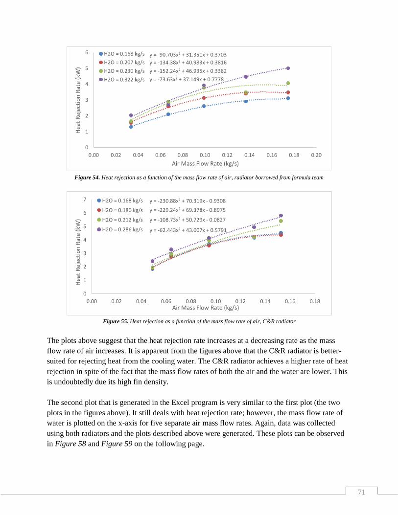
71
The plots above suggest that the heat rejection rate increases at a decreasing rate as the mass
flow rate of air increases. It is apparent from the figures above that the C&R radiator is better-
suited for rejecting heat from the cooling water. The C&R radiator achieves a higher rate of heat
rejection in spite of the fact that the mass flow rates of both the air and the water are lower. This
is undoubtedly due its high fin density.
The second plot that is generated in the Excel program is very similar to the first plot (the two
plots in the figures above). It still deals with heat rejection rate; however, the mass flow rate of
water is plotted on the x-axis for five separate air mass flow rates. Again, data was collected
using both radiators and the plots described above were generated. These plots can be observed
in Figure 58 and Figure 59 on the following page.
y = -90.703x2 + 31.351x + 0.3703
y = -134.38x2 + 40.983x + 0.3816
y = -152.24x2 + 46.935x + 0.3382
y = -73.63x2 + 37.149x + 0.7778
0
1
2
3
4
5
6
0.00 0.02 0.04 0.06 0.08 0.10 0.12 0.14 0.16 0.18 0.20
Hea
t R
ejec
tio
n R
ate
(kW
)
Air Mass Flow Rate (kg/s)
H2O = 0.168 kg/s
H2O = 0.207 kg/s
H2O = 0.230 kg/s
H2O = 0.322 kg/s
Figure 54. Heat rejection as a function of the mass flow rate of air, radiator borrowed from formula team
Figure 55. Heat rejection as a function of the mass flow rate of air, C&R radiator
y = -230.88x2 + 70.319x - 0.9308
y = -229.24x2 + 69.378x - 0.8975
y = -108.73x2 + 50.729x - 0.0827
y = -62.443x2 + 43.007x + 0.5791
0
1
2
3
4
5
6
7
0.00 0.02 0.04 0.06 0.08 0.10 0.12 0.14 0.16 0.18
Hea
t R
ejec
tio
n R
ate
(kW
)
Air Mass Flow Rate (kg/s)
H2O = 0.168 kg/s
H2O = 0.180 kg/s
H2O = 0.212 kg/s
H2O = 0.286 kg/s

72
The figures above suggest that heat rejection rate increases linearly as the mass flow rate of
water increases. The lines are relatively flat, which means that the mass flow rate of water does
not play as crucial a role in heat rejection as air flow through the core. The mass flow rate of air
is a much more significant variable with respect to heat rejection, especially at low flow rates.
4. Specification Verification Checklist or DVP&R
The following section details specifications that each component should be capable of meet to
develop an accurate model that can be used to predict the size a radiator must be to achieve
adequate cooling. It also details appropriate operating conditions for each of the components.
y = 4.5693x + 0.575
y = 3.1664x + 1.8439
y = 8.0678x + 1.4878
y = 9.9728x + 1.2466
y = 12.516x + 1.0104
0
1
2
3
4
5
6
0 0.05 0.1 0.15 0.2 0.25 0.3 0.35
Hea
t R
ejec
tio
n R
ate
(kW
)
Water Mass Flow Rate (kg/s)
Air = 0.0336 kg/s
Air = 0.0671 kg/s
Air = 0.0991 kg/s
Air = 0.1367 kg/s
Air = 0.1748 kg/s
Figure 56. Heat rejection as a function of the mass flow rate of water, radiator borrowed from formula team
Figure 57. Heat rejection as a function of the mass flow rate of water, C&R radiator
y = 4.8139x + 0.9959
y = 4.3064x + 2.0368
y = 4.5238x + 2.8767
y = 6.5546x + 3.0007
y = 11.997x + 2.483
0
1
2
3
4
5
6
7
0 0.05 0.1 0.15 0.2 0.25 0.3 0.35
Hea
t R
ejec
tio
n R
ate
(kW
)
Water Mass Flow Rate (kg/s)
Air = 0.0491 kg/s
Air = 0.0643 kg/s
Air = 0.0947 kg/s
Air = 0.1311 kg/s
Air = 0.1527 kg/s

73
Dynamometer:
Thermocouples must be present on either side of the radiator to measure the temperature
drop in the cooling fluid across the radiator.
The dyno must be operable in an open loop where water is pumped from one reservoir to
the other, as opposed to a closed loop where the same water is continually pumped
through the system.
Cole-Parmer Hot Water Bath:
The pump’s flow rate must be variable up to 8 GPM (or the max flow rate of the water
pump in the formula car’s engine).
The water level should never dip below the top of the impeller in the hot water bath.
Water needs to be continually fed into the hot water bath to prevent cavitation.
The suction side of the pump should be plugged with a brass pipe plug. This pump will
be operated in an open loop, the same way the dyno will.
Test Section:
Closed cell foam must exist at the interface between the test section and each adjacent
object to maintain airtight characteristics (even with presence of vibration).
Static pressure ports should be within half an inch of the radiator core to eliminate effects
of major head losses in the ducting from the static pressure drop measurement.
Should be mounted securely, and level, so that each piece of the test section encloses the
same space on either side of the radiator.
Radiator Setup:
The radiator fins should be in good condition to measure radiator performance.
Performing measurements with a radiator with damaged fins will measure the
performance of a damaged radiator, and the radiator should not leak.
The radiator face outside of the test section ducting should be completely covered with
aluminum foil. No air should leak from the radiator core.
Fan:
Should be appropriate for testing in the entire range of airspeeds through the core that the
car will operate at.
Measuring Devices:
Verify that all equipment has been calibrated recently.
Make sure the liquid column manometer reaches equilibrium at 0” when both sides are
subject to atmospheric air pressure.
The pitot-static tube must be held vertically against the direction of airflow.
Allow thermocouple reading to reach steady state before recording values.

74
Chapter 7: Conclusions and Recommendations
The purpose of this senior project was to develop a method of aiding the Formula SAE team at
Cal Poly in designing the cooling system that will be used on the competition car. In order to
serve this purpose for years to come as cooling requirements may change, a method that could be
used in this event was chosen. The most effective way of making the aid dynamic was to design
a series of tests to determine heat rejection requirements and the ability of a hypothetical system
to reject that heat. The following conclusions and recommendations can be made based on the
process of designing and completing the tests that will be used to aid the cooling system design.
The results from testing a couple radiators can be used to conclude a few things. First, fin density
is a very significant characteristic. A radiator with a high fin density achieved higher rates of
heat rejection at equivalent fan powers. It becomes important to know the mass flow rate of the
air through the core at equivalent car speeds when determining whether to use a radiator with a
high or low fin density. The results on the wind tunnel are heavily based on the fan’s ability to
overcome the pressure drop across the radiator. If the results from Test 3 suggest that the
difference in mass flow rate of air through the two different cores are similar to the difference on
the wind tunnel, a radiator with a higher fin density may be the best option. However, if the goal
is to minimize weight, this not be beneficial because the increased fin density may increase
weight proportionally resulting in no performance gain. If a larger radiator results in higher drag
forces and the goal is to minimize drag, it may be beneficial to use a radiator with a higher fin
density. It is all very dependent on the design goals, but the testing described in this report will
be very helpful in making these decisions.
On the topic of Test 3, it is worthwhile to note that the method of developing a relationship
between the car speed and the mass flow rate of air through the core that has been developed is
not the most effective method. It is possible that the velocity profile of the air where the radiator
will go on the formula car is completely different from the velocity profile of the air where the
test was performed on a different car. It could be beneficial to develop a new method of
developing this relationship on the car. A test fixture capable of translating and anemometer
along the face of the radiator core could be developed and used on the formula car to collect the
data needed to develop this relationship. The method that has been developed is effective, but is
slightly unorthodox and isn’t the easiest way of collecting the necessary data. The newly
developed method could be used with the radiator mounted in different locations on the car to
see if the higher mass flow rates can be achieved at slightly different spots around the car. It
could also be used to determine whether or not mounting the radiator at different angles makes a
significant difference in the mass flow rate of air through the core.
While the mass flow rate of the air through the radiator core may or may not be heavily affected
by unique velocity profiles around the car, it was very much so affected by damaged fins. Results

75
from Test 4 suggest that damaged fins can entirely eliminate air flow through the core. This
would be highly problematic with respect to cooling as that entire area of the radiator would be
rendered useless. This goes to show the extent of the benefit of having a higher fin density.
Higher rates of heat rejection were achieved in the case of the C&R radiator even with 1/3 of the
heat transfer area eliminated. While the mass flow rate of air through the core wouldn’t change
as much, the effective heat transfer area was significantly lower, so it can be concluded that the
C&R core is undoubtedly markedly more effective than the other radiator tested.
It can be concluded from the data that heat rejection rates are highly dependent on the mass flow
rate of air through the core; it is more dependent on the mass flow rate of the air than the flow
rate of the water. As such, it is possible that the worst case scenario exists at an engine power
below the maximum when the speed of the car is especially low. Data should be taken at all
crank speeds from idle to max power. It is also very likely that the worst case scenario exists at
idle and a fan will need to be use. In that case the radiator should be sized with this fact in mind.
The mass flow rate necessary to achieve adequate cooling can be determined and a fan chosen.
Then the decision to run the fan during the race must be used. If the fan is run during the race,
power from the engine will go to running the fan as opposed to turning the wheels. It will need to
be determined if the extra mass flow rate or the extra engine power is more highly valued.
The process of sizing the radiator by determining the necessary rate of heat rejection and the heat
rejected per unit of heat transfer area is based on the assumption that the rate at which heat is
rejected from the radiator increases linearly with heat transfer area. The validity of this
assumption could be tested by using aluminum foil to block off a portion of the fins in the duct
while performing Test 4 and Test 5. This would effectively test the effect relationship between
heat transfer area and heat rejection. It could also be interesting to block off horizontal then
vertical areas to determine whether the radiator orientation effects the heat rejection rate.
Finally, it should be noted that in general, if two radiators are being used they should be plumbed
in series. As detailed, in Radiator Installation in FSAE Application (Chapter 2, Section 5) when
two radiators are connected in parallel, one must pay special attention to be sure that the fluid
resistance of the two paths to each of the radiators is equal. This is the only way that the mass
flow rate of cooling water to each of the two radiators will be equal. If there is a large disparity
in the fluid resistances associated with the two parallel paths, the mass flow rate to one of the
radiators can be limited to the point of that radiator becoming extremely ineffective, vastly
prohibiting the cooling systems proficiency. This is an issue that the formula team encountered
in 2014 when two radiators were working together in a parallel configuration. While two
radiators in parallel can work more effectively, it can cause issues if not implemented properly,
and a series configuration is generally recommended.

76
Appendix A: Gantt Chart
Table 10. Gantt chart describing project timeline

77
Appendix B: Decision Matrices, QFD
The decision matrix in Table 2 below was used to verify that choosing Concept 4 described in
Conceptual Designs (Chapter 3, Section 1) was the most practical option. Each concept was
graded for the given characteristic on a scale from 1-4. They were essentially ranked from best to
worst for each of the 4 concepts. When a concept was no more effective than one of the other
concepts for a particular characteristic, they were given the same scores.
Table 11. Decision matrix used in concept selection
Table 2 indicates that using the wind tunnel in the Thermal Science Lab was the most practical
option by a wide margin. For this reason, there was no reason to add weight to each of the
characteristics. The reasons for the grades are quite predictable except for in the case of the air
speed measurement range characteristic. The LFE can only read very low air speeds in the case
of the necessary measurement range, so Concept 1 was assigned a grade of 1. Then Concept 2
and Concept 3 were assigned a grade of 2 based on the fact that there was no chance that a fan as
large as the one used on the wind tunnel in the Thermal Science Lab could be used on a flow
bench constructed for the formula team. For this reason, those two concepts would not allow for
as large a range of air speed operation. Concept 4 was assigned a grade of 4 because it was
clearly the best option in the case of this characteristic by a fairly significant margin.
A QFD that outlines the dependency of certain operating characteristics on overall design
performance can be observed on the following page. A grade of 9 indicates a strong correlation
between a characteristic and performance while, a grade of 3 indicates a medium correlation, a
grade of 1 indicates a small correlation, and a blank cell indicates no correlation.

78
Table 12. QFD for use of the ME Thermal Science Lab wind tunnel to perform radiator characterization testing

79
Appendix C: Fan Sizing Program Calculations
The following equations were used to determine the necessary pressure rise across the fan used
in testing that correlates to the maximum air mass flow rate to be tested. Equations and further
description of the way they were used follow.
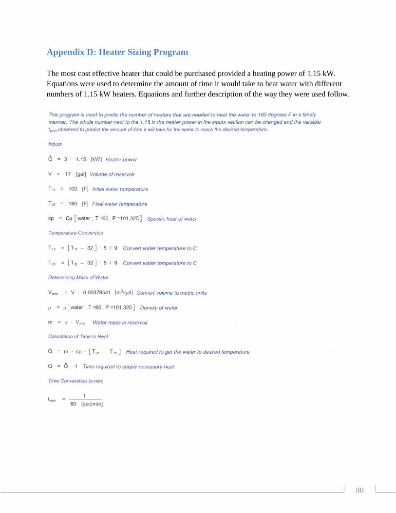
80
Appendix D: Heater Sizing Program
The most cost effective heater that could be purchased provided a heating power of 1.15 kW.
Equations were used to determine the amount of time it would take to heat water with different
numbers of 1.15 kW heaters. Equations and further description of the way they were used follow.

81

82
Appendix E: Temperature Effects on Manometer Reading
Analysis was performed to determine if the changing in the density of air due to temperature rise
across the radiator core would have a significant effect on the liquid column manometer height.
The following equations were used to generate the plot shown in Figure 21.

83
Appendix F: Cost Analysis Table
Table 13. Cost of each component used throughout the project- "cost" column includes 8.0% tax

84
Appendix G: Bills of Materials & Manufacturing/Vendor Drawings
Bill of Materials, manufacturing/vendor drawings, and vendor catalog pages will begin on the
following page.

85

86

87

88

89

90

91

92

93

94

95

96

97

98

99

100

101

102

103

104

105

106

107

108

109

110

111

112

113

114

115
116

117

118

119

120

121

122

123
Figure 58. Plumbing at radiator outlet- thermocouple and valve
Table 14. Bill of materials corresponding to above figure
Vendor catalog pages descriptions are included in the following pages.
1
2 7
5
3
6 4

124

125

126

127

128

129

130
Figure 59. Plumbing at pump discharge to couple pump discharge fitting to hose
Table 15. Bill of materials corresponding to above figure
Vendor catalog pages descriptions are included in the following pages.
1 2 3 4 6 5
131

132

133

134
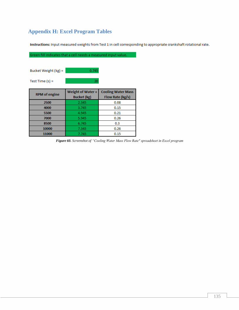
135
Appendix H: Excel Program Tables
Figure 60. Screenshot of “Cooling Water Mass Flow Rate" spreadsheet in Excel program

136
Figure 61. Screenshot of "Heat Rej. to Water" spreadsheet from Excel program

137
Figure 62. Screenshot of "Core Air Flow" spreadsheet from Excel program

138
Figure 63. Screenshot of "Core Pressure Drop" spreadsheet from Excel program

139
Figure 64. Screenshot of "Heat Rej. from Radiator" spreadsheet from Excel program

140
Appendix I: Testing Flowchart
Figure 65. Flowchart to guide user through application of test results

141
Appendix J: References
2013 Formula SAE Rules. Fsae.co. 4/29/2013.
Hastings, Jesse. “Analysis and Design of FSAE Racecar Cooling System.” 2011.
Jama, H. “Airflor Distribution through the Radiator of a Typical Australian Passenger Car.”
2004.
LFE User Manual, Meriam Company, 2013
Mullisen, Ron. “Physical Experiments in Heat Transfer and Thermodynamics.” 2011.
Callister, J., Costa, T., and George, A., "The Design of Automobile and Racing Car Cooling
Systems," SAE Technical Paper 971835, 1997.
Fujikake, Keji, Haruo Katagiri, and Yoshiaki Suzuki. "Measurement of Air Velocity Distribution
and Airflow Rate Through Radiator in an Automobile." Measurement of Air Velocity
Distribution and Airflow Rate Through Radiator in an Automobile. SAE, 01 Feb. 1978.
Web. 2013.
A.R. Khot, D.G. Thombare, S.P. Gaikwad, A.S. Adadande. “An Overview of Radiator
Performance Evaluation and Testing.” An Overview of Radiator Performance Evaluation
and Testing. ISO, 2007. Web. 2013.
Bruce R. Munson, Donald F. Young, Theodore H. Okiishi. “Fundamentals of Fluid Mechanics,
6th Edition.” John Wiley & Sons, 2009.
Frank P. Incropera, David P. Dewitt, Theodore L. Bergman, Adrienne S. Lavine. “Introduction
to Heat Transfer.” John Wiley & Sons, 2011.
H. Jama, S. Watkins, C. Dixon, E. Ng. “Airflow Distribution through the Radiator of a Typical
Passenger Car.” Airflow Distribution through the Radiator of a Typical Passenger Car.
AFMS, 2004. Web. 2013.