forecasting using - rob j hyndman · outline 1stationarity 2ordinary differencing 3seasonal...
TRANSCRIPT

Forecasting using
8. Stationarity and Differencing
OTexts.com/fpp/8/1
Forecasting using R 1
Rob J Hyndman

Outline
1 Stationarity
2 Ordinary differencing
3 Seasonal differencing
4 Unit root tests
5 Backshift notation
Forecasting using R Stationarity 2

Stationarity
DefinitionIf {yt} is a stationary time series, then for
all s, the distribution of (yt, . . . , yt+s) does
not depend on t.
A stationary series is:
roughly horizontal
constant variance
no patterns predictable in the long-term
Forecasting using R Stationarity 3

Stationarity
DefinitionIf {yt} is a stationary time series, then for
all s, the distribution of (yt, . . . , yt+s) does
not depend on t.
A stationary series is:
roughly horizontal
constant variance
no patterns predictable in the long-term
Forecasting using R Stationarity 3

Stationarity
DefinitionIf {yt} is a stationary time series, then for
all s, the distribution of (yt, . . . , yt+s) does
not depend on t.
A stationary series is:
roughly horizontal
constant variance
no patterns predictable in the long-term
Forecasting using R Stationarity 3

Stationarity
DefinitionIf {yt} is a stationary time series, then for
all s, the distribution of (yt, . . . , yt+s) does
not depend on t.
A stationary series is:
roughly horizontal
constant variance
no patterns predictable in the long-term
Forecasting using R Stationarity 3

Stationary?
Forecasting using R Stationarity 4
Day
Dow
−Jo
nes
inde
x
0 50 100 150 200 250 300
3600
3700
3800
3900

Stationary?
Forecasting using R Stationarity 5
Day
Cha
nge
in D
ow−
Jone
s in
dex
0 50 100 150 200 250 300
−10
0−
500
50

Stationary?
Forecasting using R Stationarity 6
Annual strikes in the US
Year
Num
ber
of s
trik
es
1950 1955 1960 1965 1970 1975 1980
3500
4000
4500
5000
5500
6000

Stationary?
Forecasting using R Stationarity 7
Sales of new one−family houses, USA
Tota
l sal
es
1975 1980 1985 1990 1995
3040
5060
7080
90

Stationary?
Forecasting using R Stationarity 8
Price of a dozen eggs in 1993 dollars
Year
$
1900 1920 1940 1960 1980
100
150
200
250
300
350

Stationary?
Forecasting using R Stationarity 9
Number of pigs slaughtered in Victoria
thou
sand
s
1990 1991 1992 1993 1994 1995
8090
100
110

Stationary?
Forecasting using R Stationarity 10
Annual Canadian Lynx trappings
Time
Num
ber
trap
ped
1820 1840 1860 1880 1900 1920
010
0020
0030
0040
0050
0060
0070
00

Stationary?
Forecasting using R Stationarity 11
Australian quarterly beer production
meg
alite
rs
1995 2000 2005
400
450
500

Stationary?
Forecasting using R Stationarity 12
Annual monthly electricity production
Year
GW
h
1960 1970 1980 1990
2000
6000
1000
014
000

Stationarity
DefinitionIf {yt} is a stationary time series, then for
all s, the distribution of (yt, . . . , yt+s) does
not depend on t.
Transformations help to stabilize the
variance.
For ARIMA modelling, we also need to
stabilize the mean.Forecasting using R Stationarity 13

Stationarity
DefinitionIf {yt} is a stationary time series, then for
all s, the distribution of (yt, . . . , yt+s) does
not depend on t.
Transformations help to stabilize the
variance.
For ARIMA modelling, we also need to
stabilize the mean.Forecasting using R Stationarity 13

Stationarity
DefinitionIf {yt} is a stationary time series, then for
all s, the distribution of (yt, . . . , yt+s) does
not depend on t.
Transformations help to stabilize the
variance.
For ARIMA modelling, we also need to
stabilize the mean.Forecasting using R Stationarity 13

Non-stationarity in the mean
Identifying non-stationary series
time plot.
The ACF of stationary data drops to
zero relatively quickly
The ACF of non-stationary data
decreases slowly.
For non-stationary data, the value of r1is often large and positive.
Forecasting using R Stationarity 14

Non-stationarity in the mean
Identifying non-stationary series
time plot.
The ACF of stationary data drops to
zero relatively quickly
The ACF of non-stationary data
decreases slowly.
For non-stationary data, the value of r1is often large and positive.
Forecasting using R Stationarity 14

Non-stationarity in the mean
Identifying non-stationary series
time plot.
The ACF of stationary data drops to
zero relatively quickly
The ACF of non-stationary data
decreases slowly.
For non-stationary data, the value of r1is often large and positive.
Forecasting using R Stationarity 14

Non-stationarity in the mean
Identifying non-stationary series
time plot.
The ACF of stationary data drops to
zero relatively quickly
The ACF of non-stationary data
decreases slowly.
For non-stationary data, the value of r1is often large and positive.
Forecasting using R Stationarity 14

Example: Dow-Jones index
Forecasting using R Stationarity 15
Dow Jones index (daily ending 15 Jul 94)
0 50 100 150 200 250
3600
3700
3800
3900

Example: Dow-Jones index
Forecasting using R Stationarity 16
−0.
20.
00.
20.
40.
60.
81.
0
Lag
AC
F
1 2 3 4 5 6 7 8 9 10 12 14 16 18 20 22
Example: Dow-Jones index
Forecasting using R Stationarity 17
Day
Cha
nge
in D
ow−
Jone
s in
dex
0 50 100 150 200 250 300
−10
0−
500
50

Example: Dow-Jones index
Forecasting using R Stationarity 18
−0.
15−
0.05
0.05
0.10
0.15
Lag
AC
F
1 2 3 4 5 6 7 8 9 10 12 14 16 18 20 2211 13 15 17 19 21 23

Outline
1 Stationarity
2 Ordinary differencing
3 Seasonal differencing
4 Unit root tests
5 Backshift notation
Forecasting using R Ordinary differencing 19

Differencing
Differencing helps to stabilize the
mean.
The differenced series is the change
between each observation in the
original series: y′t = yt − yt−1.
The differenced series will have only
T − 1 values since it is not possible to
calculate a difference y′1 for the first
observation.
Forecasting using R Ordinary differencing 20

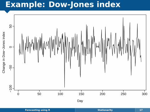
Example: Dow-Jones indexThe differences of the Dow-Jones index
are the day-today changes.
Now the series looks just like a white
noise series:no autocorrelations outside the 95% limits.Ljung-Box Q∗ statistic has a p-value 0.153 forh = 10.
Conclusion: The daily change in the
Dow-Jones index is essentially a
random amount uncorrelated with
previous days.Forecasting using R Ordinary differencing 21

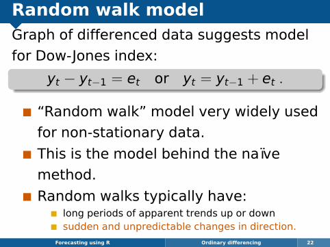
Random walk modelGraph of differenced data suggests model
for Dow-Jones index:
yt − yt−1 = et or yt = yt−1 + et .
“Random walk” model very widely used
for non-stationary data.
This is the model behind the naïve
method.
Random walks typically have:long periods of apparent trends up or downsudden and unpredictable changes in direction.
Forecasting using R Ordinary differencing 22

Random walk with drift model
yt − yt−1 = c + et or yt = c + yt−1 + et .
c is the average change between
consecutive observations.
This is the model behind the drift
method.
Forecasting using R Ordinary differencing 23

Random walk with drift model
yt − yt−1 = c + et or yt = c + yt−1 + et .
c is the average change between
consecutive observations.
This is the model behind the drift
method.
Forecasting using R Ordinary differencing 23

Random walk with drift model
yt − yt−1 = c + et or yt = c + yt−1 + et .
c is the average change between
consecutive observations.
This is the model behind the drift
method.
Forecasting using R Ordinary differencing 23
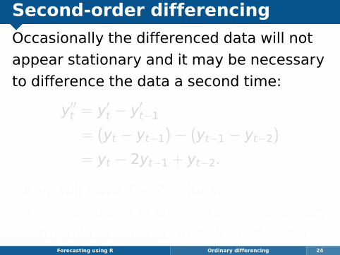
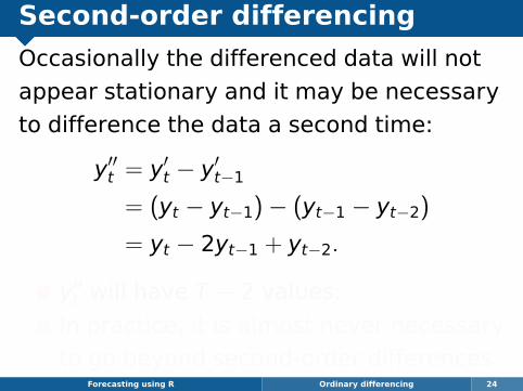
Second-order differencing
Occasionally the differenced data will not
appear stationary and it may be necessary
to difference the data a second time:
y′′t = y′t − y′t−1
= (yt − yt−1)− (yt−1 − yt−2)
= yt − 2yt−1 + yt−2.
y′′t will have T − 2 values.
In practice, it is almost never necessary
to go beyond second-order differences.Forecasting using R Ordinary differencing 24

Outline
1 Stationarity
2 Ordinary differencing
3 Seasonal differencing
4 Unit root tests
5 Backshift notation
Forecasting using R Seasonal differencing 25

Seasonal differencing
A seasonal difference is the difference
between an observation and the
corresponding observation from the
previous year.
y′t = yt − yt−m
where m = number of seasons.
For monthly data m = 12.
For quarterly data m = 4.Forecasting using R Seasonal differencing 26

Seasonal differencing
A seasonal difference is the difference
between an observation and the
corresponding observation from the
previous year.
y′t = yt − yt−m
where m = number of seasons.
For monthly data m = 12.
For quarterly data m = 4.Forecasting using R Seasonal differencing 26

Seasonal differencing
A seasonal difference is the difference
between an observation and the
corresponding observation from the
previous year.
y′t = yt − yt−m
where m = number of seasons.
For monthly data m = 12.
For quarterly data m = 4.Forecasting using R Seasonal differencing 26

Seasonal differencing
A seasonal difference is the difference
between an observation and the
corresponding observation from the
previous year.
y′t = yt − yt−m
where m = number of seasons.
For monthly data m = 12.
For quarterly data m = 4.Forecasting using R Seasonal differencing 26

Antidiabetic drug sales
Forecasting using R Seasonal differencing 27
Antidiabetic drug sales
Year
$ m
illio
n
1995 2000 2005
510
1520
2530
> plot(a10)

Antidiabetic drug sales
Forecasting using R Seasonal differencing 28
Log Antidiabetic drug sales
Year
1995 2000 2005
1.0
1.5
2.0
2.5
3.0
> plot(log(a10))

Antidiabetic drug sales5
1015
2025
30
Sal
es (
$mill
ion)
1.0
1.5
2.0
2.5
3.0
Mon
thly
log
sale
s
−0.
10.
00.
10.
20.
3
1995 2000 2005Ann
ual c
hang
e in
mon
thly
log
sale
s
Year
Antidiabetic drug sales
Forecasting using R Seasonal differencing 29
> plot(diff(log(a10),12))

Electricity production
Forecasting using R Seasonal differencing 30
Year
Bill
ion
kWh
1980 1990 2000 2010
150
200
250
300
350
400
> plot(usmelec)

Electricity production
Forecasting using R Seasonal differencing 31
Year
Logs
1980 1990 2000 2010
5.0
5.2
5.4
5.6
5.8
6.0
> plot(log(usmelec))

Electricity production
Forecasting using R Seasonal differencing 32
Year
Sea
sona
lly d
iffer
ence
d lo
gs
1980 1990 2000 2010
−0.
050.
000.
050.
100.
15
> plot(diff(log(usmelec),12))

Electricity production
Forecasting using R Seasonal differencing 33
Year
Dou
bly
diffe
renc
ed lo
gs
1980 1990 2000 2010
−0.
10−
0.05
0.00
0.05
0.10
> plot(diff(diff(log(usmelec),12),1))
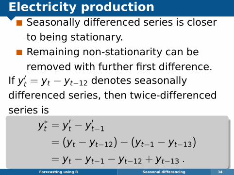
Electricity productionSeasonally differenced series is closer
to being stationary.
Remaining non-stationarity can be
removed with further first difference.If y′t = yt − yt−12 denotes seasonally
differenced series, then twice-differenced
series is
y∗t = y′t − y′t−1
= (yt − yt−12)− (yt−1 − yt−13)
= yt − yt−1 − yt−12 + yt−13 .Forecasting using R Seasonal differencing 34

Seasonal differencing
When both seasonal and first differences areapplied. . .
it makes no difference which is done first—theresult will be the same.
If seasonality is strong, we recommend thatseasonal differencing be done first becausesometimes the resulting series will bestationary and there will be no need for furtherfirst difference.
It is important that if differencing is used, thedifferences are interpretable.
Forecasting using R Seasonal differencing 35

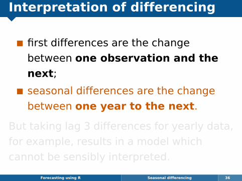
Interpretation of differencing
first differences are the change
between one observation and the
next;
seasonal differences are the change
between one year to the next.
But taking lag 3 differences for yearly data,
for example, results in a model which
cannot be sensibly interpreted.
Forecasting using R Seasonal differencing 36

Outline
1 Stationarity
2 Ordinary differencing
3 Seasonal differencing
4 Unit root tests
5 Backshift notation
Forecasting using R Unit root tests 37

Unit root tests
Statistical tests to determine the
required order of differencing.
1 Augmented Dickey Fuller test: null
hypothesis is that the data are
non-stationary and non-seasonal.
2 Kwiatkowski-Phillips-Schmidt-Shin
(KPSS) test: null hypothesis is that the
data are stationary and non-seasonal.
3 Other tests available for seasonal data.Forecasting using R Unit root tests 38
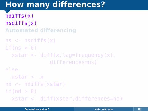
How many differences?ndiffs(x)nsdiffs(x)Automated differencing
ns <- nsdiffs(x)if(ns > 0)
xstar <- diff(x,lag=frequency(x),differences=ns)
elsexstar <- x
nd <- ndiffs(xstar)if(nd > 0)
xstar <- diff(xstar,differences=nd)
Forecasting using R Unit root tests 39
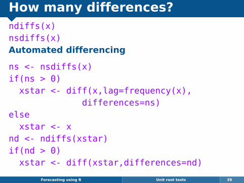
How many differences?ndiffs(x)nsdiffs(x)Automated differencing
ns <- nsdiffs(x)if(ns > 0)
xstar <- diff(x,lag=frequency(x),differences=ns)
elsexstar <- x
nd <- ndiffs(xstar)if(nd > 0)
xstar <- diff(xstar,differences=nd)
Forecasting using R Unit root tests 39

Outline
1 Stationarity
2 Ordinary differencing
3 Seasonal differencing
4 Unit root tests
5 Backshift notation
Forecasting using R Backshift notation 40

Backshift notationA very useful notational device is the backward shiftoperator, B, which is used as follows:
Byt = yt−1 .
In other words, B, operating on yt, has the effect ofshifting the data back one period. Twoapplications of B to yt shifts the data back twoperiods:
B(Byt) = B2yt = yt−2 .
For monthly data, if we wish to shift attention to“the same month last year,” then B12 is used, andthe notation is B12yt = yt−12.
Forecasting using R Backshift notation 41

Backshift notationThe backward shift operator is convenient fordescribing the process of differencing. A firstdifference can be written as
y′t = yt − yt−1 = yt − Byt = (1− B)yt .
Note that a first difference is represented by (1−B).Similarly, if second-order differences (i.e., firstdifferences of first differences) have to becomputed, then:
y′′t = yt − 2yt−1 + yt−2 = (1− B)2yt .
Forecasting using R Backshift notation 42

Backshift notation
Second-order difference is denoted (1− B)2.
Second-order difference is not the same as asecond difference, which would be denoted1− B2;
In general, a dth-order difference can bewritten as
(1− B)dyt.
A seasonal difference followed by a firstdifference can be written as
(1− B)(1− Bm)yt .
Forecasting using R Backshift notation 43

Backshift notation
The “backshift” notation is convenient because theterms can be multiplied together to see thecombined effect.
(1− B)(1− Bm)yt = (1− B− Bm + Bm+1)yt= yt − yt−1 − yt−m + yt−m−1.
For monthly data, m = 12 and we obtain the sameresult as earlier.
Forecasting using R Backshift notation 44