finite differencing of logical formulas for static analysis
TRANSCRIPT
Finite Differencing of Logical Formulas
for Static Analysis
THOMAS REPS
University of Wisconsin and GrammaTech, Inc.
MOOLY SAGIV
Tel Aviv University
and
ALEXEY LOGINOV
GrammaTech, Inc.
This paper concerns mechanisms for maintaining the value of an instrumentation relation (alsoknown as a derived relation or view), defined via a logical formula over core relations, in responseto changes in the values of the core relations. It presents an algorithm for transforming theinstrumentation relation’s defining formula into a relation-maintenance formula that captureswhat the instrumentation relation’s new value should be. The algorithm runs in time linear inthe size of the defining formula.
The technique applies to program-analysis problems in which the semantics of statements isexpressed using logical formulas that describe changes to core-relation values. It provides a wayto obtain values of the instrumentation relations that reflect the changes in core-relation values
produced by executing a given statement.We present experimental evidence that our technique is an effective one: for a variety of bench-
marks, the relation-maintenance formulas produced automatically using our approach yield thesame precision as the best available hand-crafted ones.
Categories and Subject Descriptors: D.2.4 [Software Engineering]: Software/Program Verifica-tion—formal methods; D.3.3 [Programming Languages]: Language Constructs and Features—data types and structures; dynamic storage management; E.1 [Data]: Data Structures—graphsand networks; lists, stacks, and queues; records; trees; E.2 [Data]: Data Storage Representa-tions—composite structures; linked representations; F.3.1 [Logics and Meanings of Programs]:Specifying and Verifying and Reasoning about Programs—assertions; invariants; mechanical ver-ification; F.3.2 [Logics and Meanings of Programs]: Semantics of Programming Languages—program analysis
General Terms: Algorithms, Languages, Theory, Verification
Additional Key Words and Phrases: Abstract interpretation, finite differencing, materialized view,shape analysis, static analysis, 3-valued logic
Authors’ addresses: T. Reps, Comp. Sci. Dept., University of Wisconsin, and GrammaTech, Inc.,[email protected]. M. Sagiv, School of Comp. Sci., Tel Aviv University, [email protected]. Loginov, GrammaTech, Inc., [email protected]. At the time the research reported inthe paper was carried out, A. Loginov was affiliated with the Univ. of Wisconsin.
The work was supported in part by NSF under grants CCR-{9619219,9986308}, and CCF-{0540955,0524051}, by the U.S.-Israel BSF under grant 96-00337, by ONR under contractsN00014-01-1-{0708,0796}, and by the von Humboldt and Guggenheim Foundations. Portions ofthe work appeared in the 12th European Symp. on Programming [Reps et al. 2003], R. Wilhelm’s60th-birthday Festschrift [Loginov et al. 2007], and A. Loginov’s Ph.D. dissertation [Loginov 2006].c© 2009 T. Reps, M. Sagiv, and A. Loginov

2 · T. Reps et al.
1. INTRODUCTION
This paper addresses an instance of the following fundamental challenge in abstractinterpretation:
Given the concrete semantics for a language and a desired abstraction,how does one create the associated abstract transformers?
The problem that we address arises in program-analysis problems in which the se-mantics of statements is expressed using logical formulas that describe changes tocore-relation values. When instrumentation relations (defined via logical formulasover the core relations) have been introduced to refine an abstraction, the challengeis to develop a method for obtaining values of the instrumentation relations thatreflect the changes in core-relation values [Graf and Saıdi 1997; Das et al. 1999;McMillan 1999; Sagiv et al. 2002; Ball et al. 2001]. The algorithm presented inthis paper provides a way to create formulas that maintain correct values for theinstrumentation relations, and thereby provides a way to generate, completely au-tomatically, the part of the transformers of an abstract semantics that deals withinstrumentation relations. The algorithm runs in time linear in the size of theinstrumentation relation’s defining formula.
This research was motivated by our work on static analysis based on 3-valuedlogic [Sagiv et al. 2002]; however, any analysis method that relies on logic—2-valuedor 3-valued—to express a program’s semantics may be able to benefit from thesetechniques.
In our setting, two related logics come into play: an ordinary 2-valued logic, aswell as a related 3-valued logic. A memory configuration, or store, is modeled bywhat logicians call a logical structure; an individual of the structure’s universe eithermodels a single memory element or, in the case of a summary individual, it modelsa collection of memory elements. A run of the analyzer carries out an abstractinterpretation to collect a set of structures at each program point P . This involvesfinding the least fixed point of a certain set of equations. When the fixed pointis reached, the structures that have been collected at program point P describe asuperset of all the execution states that can occur at P . To determine whether aproperty always holds at P , one checks whether it holds in all of the structuresthat were collected there. Instantiations of this framework are capable of estab-lishing nontrivial properties of programs that perform complex pointer-based ma-nipulations of a priori unbounded-size heap-allocated data structures. The TVLAsystem (Three-Valued-Logic Analyzer) implements this approach [Lev-Ami andSagiv 2000; TVLA ].
Summary individuals play a crucial role. They are used to ensure that abstractdescriptors have an a priori bounded size, which guarantees that a fixed-point isalways reached. However, the constraint of working with limited-size descriptorsimplies a loss of information about the store. Intuitively, certain properties ofconcrete individuals are lost due to abstraction, which groups together multipleindividuals into summary individuals: a property can be true for some concreteindividuals of the group but false for other individuals. It is for this reason that3-valued logic is used; uncertainty about a property’s value is captured by meansof the third truth value, 1/2.

Finite Differencing of Logical Formulas · 3
An advantage of using 2- and 3-valued logic as the basis for static analysis is thatthe language used for extracting information from the concrete world and the ab-stract world is identical: every syntactic expression—i.e., every logical formula—canbe interpreted either in the 2-valued world or the 3-valued world. The consistencyof the 2-valued and 3-valued viewpoints is ensured by a basic theorem that relatesthe two logics [Sagiv et al. 2002, Theorem 4.9]. This provides a partial answer tothe fundamental challenge posed above: formulas that define the concrete seman-tics, when interpreted in 2-valued logic, define a sound abstract semantics wheninterpreted in 3-valued logic [Sagiv et al. 2002].
Unfortunately, unless some care is taken in the design of an analysis, there isa danger that as abstract interpretation proceeds, the indefinite value 1/2 will be-come pervasive. This can destroy the ability to recover interesting information fromthe 3-valued structures collected (although soundness is maintained). A key role incombating indefiniteness is played by instrumentation relations, which record aux-iliary information in a logical structure. The benefit of introducing instrumentationrelations was annunciated as the Instrumentation Principle:
Observation 1.1. (Instrumentation Principle [Sagiv et al. 2002, Obser-vation 2.8]). Suppose that S# is a 3-valued structure that represents the 2-valuedstructure S. By explicitly “storing” in S# the values that a formula ψ has in S,it is sometimes possible to extract more precise information from S# than can beobtained just by evaluating ψ in S#. 2
Instrumentation relations provide a mechanism to fine-tune an abstraction: an in-strumentation relation, which is defined by a logical formula ψ over the core-relationsymbols, captures a property that may or may not be possessed by a structure, anindividual memory cell, or a tuple of memory cells (according to whether ψ is anullary, unary, or k-ary formula, respectively). For instance, the following formulasdefine nullary, unary, and binary instrumentation relations relating to cycles (oflength one or more) along n edges, where the ∗ operator denotes transitive closure:
Nullary (Does the structure contain a cycle?): ψc0()def= ∃v1, v2 : n(v1, v2) ∧ n
∗(v2, v1)
Unary (Is v1 on a cycle?): ψc1(v1)def= ∃v2 : n(v1, v2) ∧ n
∗(v2, v1)
Binary (Is n edge v1 → v2 part of a cycle?): ψc2(v1, v2)def= n(v1, v2) ∧ n
∗(v2, v1)
In general, the introduction of additional instrumentation relations refines an ab-straction into one that is prepared to track finer distinctions among stores. Forreasons discussed in §3, the values of instrumentation relations are stored and main-tained in response to the store transformations performed by program statements.In many cases, this technique allows more precise properties of the program’s storesto be established.
Problem Statement and Contributions. From the standpoint of the concrete se-mantics, instrumentation relations represent cached information that could alwaysbe recomputed by reevaluating the instrumentation relation’s defining formula inthe local state. From the standpoint of the abstract semantics, however, reevaluat-ing a formula in the local (3-valued) state can lead to a drastic loss of precision. Togain maximum benefit from instrumentation relations, an abstract-interpretationalgorithm must obtain their values in some other way. We call this problem the

4 · T. Reps et al.
instrumentation-relation-maintenance problem (often shortened to the “relation-maintenance problem”). To summarize, the problem that we address is the fol-lowing:
Given a formula ψp that defines an instrumentation relation p, togetherwith formulas τc that specify how each core relation c is transformed bytransformer τ , create a relation-maintenance formula for p.
To reduce the loss of precision, the solution to the relation-maintenance problemdeveloped in this paper uses an incremental-computation strategy. After a tran-sition via transformer τ from abstract state σ to abstract state σ′, the new valuethat instrumentation relation p should have is computed from the stored value ofp in σ.
The contributions of the work reported in the paper can be summarized as follows:
—We give an algorithm for solving the relation-maintenance problem. The al-gorithm works by applying a finite-differencing transformation to p’s definingformula ψp. The algorithm runs in time linear in the size of ψp.
—We present experimental evidence that our technique is an effective one, at leastfor the analysis of programs that manipulate (cyclic and acyclic) singly-linkedlists, doubly-linked lists, and binary trees, and for certain sorting programs. Inparticular, the relation-maintenance formulas produced automatically using ourapproach are as effective for maintaining precision as the best available hand-crafted ones.
Organization. The remainder of the paper is organized as follows: §2 introducesterminology and notation. §3 defines the relation-maintenance problem. §4 pro-vides intuition behind our solution, which is presented in §5 and §6. §5 presentsa method for generating maintenance formulas for instrumentation relations. §6discusses extensions to handle instrumentation relations that use transitive closure.§7 presents experimental results. §8 discusses related work. §9 presents someconcluding remarks. Finally, the Appendix presents a proof of the correctness ofour solution to the relation-maintenance problem.
2. BACKGROUND
This section introduces terminology and notation; it presents the logic that weemploy and describes the use of logical structures for representing memory stores.
The first half of §2.1 introduces 2-valued first-order logic with transitive closure.These concepts are standard in logic. The second half of §2.1 presents a straightfor-ward extension of the logic to the 3-valued setting, in which a third truth value—1/2—is introduced to denote uncertainty. §2.2 summarizes the program-analysisframework described in [Sagiv et al. 2002]. In that approach, memory configura-tions are encoded as 2-valued logical structures. The semantics of programs, as wellas properties of memory configurations, are encoded using formulas. Abstract inter-pretation [Cousot and Cousot 1977] is performed to compute, at each point in theprogram being analyzed, a set of 3-valued logical structures that over-approximatesthe memory configurations that can arise at that point.
Finite Differencing of Logical Formulas · 5
2.1 First-Order Logic with Transitive Closure
2-Valued First-Order Logic with Transitive Closure. The syntax of first-orderformulas with equality and reflexive transitive closure is defined as follows:
Definition 2.1. Let Ri denote a set of arity-i relation symbols,1 with eq ∈ R2.A formula over the vocabulary R =
⋃
i Ri is defined by
p ∈ Rk ϕ ::= 0 | 1 | p(v1, . . . , vk)ϕ ∈ Formulas | (¬ϕ1) | (ϕ1 ∧ ϕ2) | (ϕ1 ∨ ϕ2) | (∃v : ϕ1) | (∀v : ϕ1)v ∈ Variables | (RTC v′1, v
′2 : ϕ1)(v1, v2)
A formula of the form 0, 1, or p(v1, . . . , vk) is called an atomic formula.The set of free variables of a formula is defined as usual. “RTC” stands for
reflexive transitive closure. In ϕ ≡ (RTC v′1, v′2 : ϕ1)(v1, v2), if ϕ1’s free-variable
set is V , we require v1, v2 6∈ V . The free variables of ϕ are (V −{v′1, v′2})∪{v1, v2}.
2
We use several shorthand notations: (v1 =v2)def
= eq(v1, v2); (v1 6=v2)def
= ¬eq(v1, v2);
and for a binary relation p, p∗(v1, v2)def
= (RTC v′1, v′2 : p(v′1, v
′2))(v1, v2). We also
use a C-like syntax for conditional expressions: ϕ1 ? ϕ2 : ϕ3.2 The order of prece-
dence among the connectives, from highest to lowest, is as follows: ¬, ∧, ∨, ∀, and∃. We drop parentheses wherever possible, except for emphasis.
Definition 2.2. A 2-valued interpretation over R is a 2-valued logical structureS = 〈US , ιS〉, where US is a set of individuals and ιS maps each relation symbolp ∈ Rk to a truth-valued function: ιS(p) : (US)k → {0, 1}. In addition, (i) for allu ∈ US, ιS(eq)(u, u) = 1, and (ii) for all u1, u2 ∈ US such that u1 and u2 aredistinct individuals, ιS(eq)(u1, u2) = 0.
An assignment Z is a function that maps variables to individuals (i.e., it hasthe functionality Z : {v1, v2, . . .} → US). When Z is defined on all free variablesof a formula ϕ, we say that Z is complete for ϕ. (We generally assume that ev-ery assignment that arises in connection with the discussion of some formula ϕ iscomplete for ϕ.)
The (2-valued) meaning of a formula ϕ, denoted by [[ϕ]]S2 (Z), yields a truth valuein {0, 1}; it is defined inductively as follows:
[[0]]S2 (Z) = 0 [[ϕ1 ∧ ϕ2]]S2 (Z) = min([[ϕ1]]
S2 (Z), [[ϕ2]]
S2 (Z))
[[1]]S2 (Z) = 1 [[ϕ1 ∨ ϕ2]]S2 (Z) = max([[ϕ1]]
S2 (Z), [[ϕ2]]
S2 (Z))
[[p(v1, . . . , vk)]]S2 (Z) = ιS(p)(Z(v1), . . . , Z(vk)) [[∃v : ϕ1]]S2 (Z) = max
u∈US[[ϕ1]]
S2 (Z[v 7→ u])
[[¬ϕ1]]S2 (Z) = 1− [[ϕ1]]
S2 (Z) [[∀v : ϕ1]]
S2 (Z) = min
u∈US[[ϕ1]]
S2 (Z[v 7→ u])
[[(RTC v′1, v′2 : ϕ1)(v1, v2)]]
S2 (Z)
=
1 ifZ(v1) = Z(v2)
maxn ≥ 1,
u1, . . . , un+1 ∈ U,Z(v1) = u1,
Z(v2) = un+1
nmini=1
[[ϕ1]]S2 (Z[v′1 7→ ui, v
′2 7→ ui+1]) otherwise
1Instead of introducing function symbols, we encode a function of arity i by means of a relationof arity i+ 1, together with logical constraints (described in §2.2.2 in the discussion of Fig. 10).2In 2-valued logic, one can think of ϕ1 ? ϕ2 : ϕ3 as a shorthand for (ϕ1 ∧ ϕ2) ∨ (¬ϕ1 ∧ ϕ3). In3-valued logic, it becomes a shorthand for (ϕ1 ∧ ϕ2) ∨ (¬ϕ1 ∧ ϕ3) ∨ (ϕ2 ∧ ϕ3) [Reps et al. 2002].

6 · T. Reps et al.
1/2
0
1J
JJ
Jt 0 1/2 1
0 0 1/2 1/21/2 1/2 1/2 1/21 1/2 1/2 1
1
1/2
0
∨ 0 1/2 1
0 0 1/2 11/2 1/2 1/2 11 1 1 1
(a) (b)
Fig. 1. (a) The information order (v) and its join operation (t). (b) The logical order and itsjoin operation (∨).
S and Z satisfy ϕ if [[ϕ]]S2 (Z) = 1. The set of 2-valued structures is denoted byS2[R], where “[R]” is dropped if the vocabulary R is understood. 2
3-Valued Logic and Embedding. In 3-valued logic, the formulas that we work withare identical to the ones used in 2-valued logic. At the semantic level, a third truthvalue—1/2—is introduced to denote uncertainty.
Definition 2.3. The truth values 0 and 1 are definite values ; 1/2 is an indefinitevalue. For l1, l2 ∈ {0, 1/2, 1}, the information order is defined as follows: l1 v l2iff l1 = l2 or l2 = 1/2. l1 v l2 denotes that l1 is at least as definite as l2. We usel1 @ l2 when l1 v l2 and l1 6= l2. The symbol t denotes the least-upper-boundoperation with respect to v. 2
As shown in Fig. 1, we place two orderings on 0, 1, and 1/2: (i) the informationorder, denoted by v and illustrated in Fig. 1(a), captures “(un)certainty”; (ii) thelogical order, shown in Fig. 1(b), defines the meaning of ∧ and ∨; that is, ∧ and ∨are meet and join in the logical order. 3-valued logic retains a number of propertiesthat are familiar from 2-valued logic, such as De Morgan’s laws, associativity of∧ and ∨, and distributivity of ∧ over ∨ (and vice versa). Because ϕ1 ? ϕ2 : ϕ3 istreated as a shorthand for (ϕ1 ∧ϕ2)∨ (¬ϕ1 ∧ϕ3)∨ (ϕ2 ∧ϕ3) in 3-valued logic [Repset al. 2002], the value of 1/2 ? V1 : V2 equals V1 tV2. We now generalize Defn. 2.2to define the meaning of a formula with respect to a 3-valued structure.
Definition 2.4. A 3-valued interpretation over R is a 3-valued logical structureS = 〈US , ιS〉, where US is a set of individuals and ιS maps each relation symbolp ∈ Rk to a truth-valued function: ιS(p) : (US)k → {0, 1/2, 1}. In addition, (i) forall u ∈ US , ιS(eq)(u, u) w 1, and (ii) for all u1, u2 ∈ U
S such that u1 and u2 aredistinct individuals, ιS(eq)(u1, u2) = 0.
For an assignment Z, the (3-valued) meaning of a formula ϕ, denoted by [[ϕ]]S3 (Z),yields a truth value in {0, 1/2, 1}. The meaning of ϕ is defined exactly as inDefn. 2.2, but interpreted over {0, 1/2, 1}. S and Z potentially satisfy ϕ if [[ϕ]]S3 (Z) w1. The set of 3-valued structures is denoted by S3[R], where “[R]” is dropped ifthe vocabulary R is understood. 2
Defn. 2.4 requires that for each individual u, the value of ιS(eq)(u, u) is 1 or 1/2.An individual for which ιS(eq)(u, u) = 1/2 is called a summary individual. In theprogram-analysis framework of [Sagiv et al. 2002], a summary individual abstracts

Finite Differencing of Logical Formulas · 7
x 1 8 5n n
Fig. 2. A possible store for a linked list.
one or more nodes of a data structure, and hence can represent more than oneconcrete memory cell.
The embedding ordering on structures is defined as follows:
Definition 2.5. Let S = 〈US , ιS〉 and S′ = 〈US′
, ιS′
〉 be two structures, andlet f : US → US′
be a surjective function. We say that f embeds S in S′ (denotedby S vf S′) if for every relation symbol p ∈ Rk and for all u1, . . . , uk ∈ US ,ιS(p)(u1, . . . , uk) v ιS
′
(p)(f(u1), . . . , f(uk)). We say that S can be embedded in S′
(denoted by S v S′) if there exists a function f such that S vf S′. 2
The Embedding Theorem says that if S vf S′, then every piece of informationextracted from S′ via a formula ϕ is a conservative approximation of the informationextracted from S via ϕ. To formalize this, we extend mappings on individualsto operate on assignments: if f : US → US′
is a function and Z : V ar → US
is an assignment, f ◦ Z denotes the assignment f ◦ Z : V ar → US′
such that(f ◦ Z)(v) = f(Z(v)).
Theorem 2.6. (Embedding Theorem [Sagiv et al. 2002, Theorem 4.9]).Let S = 〈US , ιS〉 and S′ = 〈US′
, ιS′
〉 be two structures, and let f : US → US′
be afunction such that S vf S′. Then, for every formula ϕ and complete assignment Zfor ϕ, [[ϕ]]S3 (Z) v [[ϕ]]S
′
3 (f ◦ Z). 2
In the rest of the paper, we will denote 2-valued structures by S (possibly withsubscripts and primes) and 3-valued structures by S# (possibly with subscripts).
2.2 Stores as Logical Structures and their Abstractions
Program Analysis Via 3-Valued Logic. The remainder of this section summarizesthe program-analysis framework described in [Sagiv et al. 2002]. In that approach,concrete memory configurations (i.e., stores) are encoded as logical structures (as-sociated with a vocabulary of relation symbols with given arities) in terms of a fixedcollection of core relations, C. Core relations are part of the underlying semantics ofthe language to be analyzed; they record atomic properties of stores. For instance,Fig. 3 gives the definition of a C linked-list datatype, and lists the relations thatwould be used to represent the stores manipulated by programs that use type List,such as the store in Fig. 2. (The core relations are fixed for a given combination oflanguage and datatype; in general, different languages and datatypes require differ-ent collections of core relations.) 2-valued logical structures then represent memoryconfigurations: the individuals of the structure are the set of memory cells; a nullaryrelation represents a Boolean variable of the program; a unary relation representseither a pointer variable or a Boolean-valued field of a record; and a binary relationrepresents a pointer field of a record. In Fig. 3, unary relations represent pointervariables, and binary relation n represents the n-field of a List cell. Numeric-valuedvariables and numeric-valued fields (such as data) can be modeled by introducingother relations, such as the binary relation dle (which stands for “data less-than-or-equal-to”) listed in Fig. 3; dle captures the relative order of two nodes’ data values.

8 · T. Reps et al.
typedef struct node {
struct node *n;
int data;
} *List;
Relation Intended Meaning
eq(v1, v2) Do v1 and v2 denote the same memory cell?x(v) Does pointer variable x point to memory cell v?n(v1, v2) Does the n field of v1 point to v2?dle(v1, v2) Is the data field of v1 less than or equal to
that of v2?
(a) (b)
Fig. 3. (a) Declaration of a linked-list datatype in C. (b) Core relations used for representing thestores manipulated by programs that use type List.
x
dle
dle
n
dle
n
dle
u1
dle
u2
dle
u3
x
u1 1
u2 0
u3 0
n u1 u2 u3
u1 0 1 0
u2 0 0 1
u3 0 0 0
dle u1 u2 u3
u1 1 1 1
u2 0 1 0
u3 0 1 1
Fig. 4. A logical structure S4 that represents the store shown in Fig. 2 in graphical and tabularforms using the relations of Fig. 3 (Relation eq is not shown explicitly; each node has an eqself-loop, and the relation in tabular form is the identity matrix.)
(Alternatively, numeric-valued entities can be handled by combining abstractions oflogical structures with previously known techniques for creating numeric abstrac-tions [Gopan et al. 2004].) Fig. 4 shows 2-valued structure S4, which represents thestore of Fig. 2 using the relations of Fig. 3. S4 has three individuals, u1, u2, andu3, which represent the three list elements.
Information about a concrete memory configuration encoded as a logical structurecan be extracted from the logical structure by evaluating formulas.
A concrete operational semantics is defined by specifying a structure transformerst(n1,n2) for each outgoing control-flow graph (CFG) edge (n1, n2). (Ordinarily(n1, n2) is understood, and we just write st.) A structure transformer is specified byproviding a collection of relation-transfer formulas, τc,st, one for each core relationc. These formulas define how the core relations of a 2-valued logical structure S1
that arises at n1 are transformed by st(n1,n2) to create a 2-valued logical structureS2 at n2; typically, they define the value of relation c in S2 as a function of c’svalue in S1 and the values of other core relations in S1. For instance, Fig. 9,described in more detail later in this section, shows that the value of unary relationy in a structure transformed by the structure transformer corresponding to thestatement y = x is defined as a function of the value of unary relation x, namely:τy,y=x(v) = x(v). We use the notation [[st]]2(S1) to denote the transformation of S1
by structure transformer st.Transformer st may optionally have a precondition formula, which filters out
structures that should not follow the transition along (n1, n2). The postconditionoperator post for edge (n1, n2) is defined by lifting (n1, n2)’s structure transformerto sets of structures.
Finite Differencing of Logical Formulas · 9
dlex
dle n,dlen
u1u23
x
u1 1
u23 0
n u1 u23
u1 0 1/2
u23 0 1/2
dle u1 u23
u1 1 1
u23 0 1/2
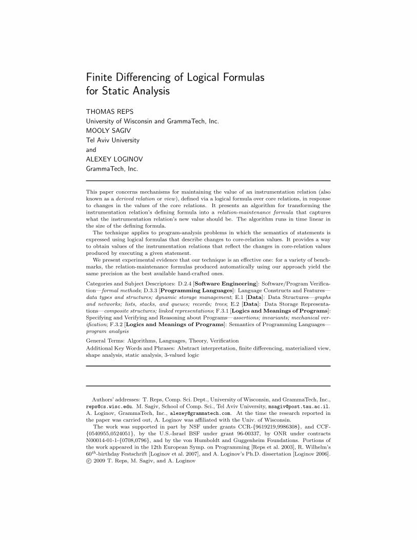
Fig. 5. A 3-valued structure S#5 that is the canonical abstraction of structure S4.
Abstract stores are 3-valued logical structures. Concrete stores are abstracted toabstract stores by means of embedding functions—onto functions that map individ-uals of a 2-valued structure S to those of a 3-valued structure S#. The EmbeddingTheorem ensures that every piece of information extracted from S# by evaluatinga formula ϕ is a conservative approximation (w) of the information extracted fromS by evaluating ϕ.
To obtain a computable abstract domain, we ensure that the size of the 3-valuedstructures used to represent memory configurations is always bounded. We do thisby defining an equivalence relation on individuals and considering the (bounded-size) quotient structure with respect to this equivalence relation; in particular,each individual of a 2-valued logical structure (representing a concrete memorycell) is mapped to an individual of a 3-valued logical structure according to thevector of values that the concrete individual has for a user-chosen collection ofunary abstraction relations. Intuitively, this equivalence relation maps a group ofindividuals, which are indistinguishable according to the set of (unary) abstractionrelations A, to a single individual:
Definition (Canonical Abstraction). Let S ∈ S2[R], and let A ⊆ R1 besome chosen (nonempty) subset of the unary relation symbols. The relations in Aare called abstraction relations ; they define the following equivalence relation 'A
on US :
u1 'A u2 ⇐⇒ for all p ∈ A, ιS(p)(u1) = ιS(p)(u2).
Additionally, abstraction relations define the surjective function fA : US → US/ 'A,such that fA(u) = [u]'A
, which maps an individual to its equivalence class. Thecanonical abstraction of S with respect to A (denoted by fA(S)) performs the join(in the information order) of relation values, thereby introducing 1/2’s: for everyp ∈ Rk,
ιfA(S)(p)(u′1, . . . , u′k) =
⊔
(u1, . . . , uk) ∈ (US)k, s.t.
fA(ui) = u′
i ∈ US/ 'A, 1 ≤ i ≤ k
ιS(p)(u1, . . . , uk) (1)
2
If A = {x}, the canonical abstraction of 2-valued logical structure S4 is S#5 ,
shown in Fig. 5, with fA(u1) = u1 and fA(u2) = fA(u3) = u23. In addition to S4,
S#5 represents any list with two or more elements that is pointed to by program
variable x, and in which the first element’s data value is (definitely) less than thedata values in the rest of the list (note the absence of either a 1-valued or 1/2-valued

10 · T. Reps et al.
p Intended Meaning ψp
isn(v) Do n fields of two or more list nodes point to v? ∃ v1, v2 : n(v1, v)∧ n(v2, v) ∧ v1 6=v2tn(v1, v2) Is v2 reachable from v1 along zero or more n fields? n∗(v1, v2)
rn,x(v) Is v reachable from pointer variable x ∃ v1 : x(v1)∧ tn(v1, v)along zero or more n fields?
cn(v) Is v on a directed cycle of n fields? ∃ v1 : n(v1, v)∧ tn(v, v1)
Fig. 6. Defining formulas of some commonly used instrumentation relations. The relation nameisn abbreviates “is-shared”. There is a separate reachability relation rn,x for every programvariable x. (Recall that v1 6=v2 is a shorthand for ¬eq(v1, v2), and n∗(v1, v2) is a shorthand for(RTC v′1, v
′
2 : n(v′1, v′
2))(v1, v2).)
dle edge from individual u23 to individual u1). The following graphical notation isused for depicting 3-valued logical structures:
—Individuals are represented by circles containing their names and (non-0) valuesfor unary relations. Summary individuals are represented by double circles.
—A unary relation p corresponding to a pointer-valued program variable is repre-sented by a solid arrow from p to the individual u for which p(u) = 1, and bythe absence of a p-arrow to each node u′ for which p(u′) = 0. (If p = 0 for allindividuals, the relation name p is not shown.)
—A binary relation q is represented by a solid arrow labeled q between each pairof individuals ui and uj for which q(ui, uj) = 1, and by the absence of a q-arrowbetween pairs u′i and u′j for which q(u′i, u
′j) = 0.
—Relations with value 1/2 are represented by dashed arrows.
Canonical abstraction ensures that each 3-valued structure is no larger than somefixed size, known a priori. While canonical abstraction is defined on 2-valued struc-tures, its operations can be applied to 3-valued structures, as well, possibly produc-ing more abstract structures (i.e., ones with fewer individuals). In a slight abuse ofterminology, we will sometimes discuss the application of canonical abstraction to3-valued structures.
2.2.1 Instrumentation Relations. The abstraction function on which an analysisis based, and hence the precision of the analysis defined, can be tuned by (i) choos-ing to equip structures with additional instrumentation relations to record derivedproperties, and (ii) varying which of the unary core and unary instrumentationrelations are used as the set of abstraction relations. The set of instrumentationrelations is denoted by I. Each arity-k relation symbol p ∈ I is defined by aninstrumentation-relation definition formula ψp(v1, . . . , vk). Instrumentation rela-tions may appear in the defining formulas of other instrumentation relations aslong as there are no circular dependences.
The introduction of unary instrumentation relations that are used as abstractionrelations provides a way to control which concrete individuals are merged togetherinto an abstract individual, and thereby control the amount of information lost byabstraction. Instrumentation relations that involve reachability properties, whichcan be defined using RTC, often play a crucial role in the definitions of abstractions.For instance, in program-analysis applications, reachability properties from specificpointer variables have the effect of keeping disjoint sublists summarized separately.

Finite Differencing of Logical Formulas · 11
x
tn,dle
tn,dle
dle
u1rn,x
tn,dle
u2rn,x
n,tn
dletn,dle
u3rn,x
n,tn
x rn,x cn
u1 1 1 0
u2 0 1 0
u3 0 1 0
n u1 u2 u3
u1 0 1 0
u2 0 0 1
u3 0 0 0
tn u1 u2 u3
u1 1 1 1
u2 0 1 1
u3 0 0 1
dle u1 u2 u3
u1 1 1 1
u2 0 1 0
u3 0 1 1
Fig. 7. A logical structure S7, which represents the store shown in Fig. 2, in graphical and tabularforms using the relations of Figs. 3 and 6.
tn,dlex
tn,dle n,tn,dlen
u1rn,x
u23rn,x
x rn,x cn
u1 1 1 0
u23 0 1 0
n u1 u23
u1 0 1/2
u23 0 1/2
tn u1 u23
u1 1 1
u23 0 1/2
dle u1 u23
u1 1 1
u23 0 1/2
Fig. 8. A 3-valued structure S#8 that is the canonical abstraction of structure S7.
Fig. 6 lists some instrumentation relations that are important for the analysis ofprograms that use type List.
Fig. 7 shows 2-valued structure S7, which represents the store of Fig. 2 usingthe core relations of Fig. 3, as well as the instrumentation relations of Fig. 6. Ifall unary relations are abstraction relations (A = R1), the canonical abstraction
of 2-valued logical structure S7 is S#8 , shown in Fig. 8, with fA(u1) = u1 and
fA(u2) = fA(u3) = u23.
2.2.2 Abstract Interpretation. For each kind of statement in the programminglanguage, the abstract semantics is again defined by a collection of formulas: thesame relation-transfer formula that defines the concrete semantics, in the case ofa core relation, and, in the case of an instrumentation relation p, by a relation-maintenance formula µp,st.
3
In our context, abstract interpretation collects a set of 3-valued structures ateach program point. It can be implemented as an iterative procedure that finds theleast fixed point of a certain set of equations [Sagiv et al. 2002]. (It is importantto understand that although the analysis framework is based on logic, it is model-theoretic, not proof-theoretic: the abstract interpretation collects sets of 3-valuedlogical structures—i.e., abstracted models; its actions do not rely on deduction or
3In [Sagiv et al. 2002], relation-transfer formulas and relation-maintenance formulas are both called“relation-update formulas”. Here we use separate terms so that we can refer easily to relation-maintenance formulas, which are the main subject of this paper. The term “relation-maintenanceformula”emphasizes the connection to work in the database community on view maintenance (see§8). (“View updating” is something different: an update is made to the value of a view relationand changes are propagated back to the base relations.)

12 · T. Reps et al.
Structure before
unary rels. binary rels.
indiv. x y
u1 1 0u 0 0
n u1 u
u1 0 1/2u 0 1/2
eq u1 u
u1 1 0u 0 1/2
x // ?>=<89:;u1n //?>=<89:;/.-,()*+u
n
��
Statement y = x
Relation-transfer formulas
τx,y=x(v) = x(v)τy,y=x(v) = x(v)
τn,y=x(v1, v2) = n(v1, v2)τeq,y=x(v1, v2) = eq(v1, v2)
Structure after
unary rels. binary rels.
indiv. x y
u1 1 1u 0 0
n u1 u
u1 0 1/2u 0 1/2
eq u1 u
u1 1 0u 0 1/2
x, y // ?>=<89:;u1n //?>=<89:;/.-,()*+u
n
��
Fig. 9. The relation-transfer formulas for x, y, and n express a transformation on logical structuresthat corresponds to the semantics of y = x.
theorem proving.) When the fixed point is reached, the structures that have beencollected at program point P describe a superset of all the execution states thatcan occur at P . To determine whether a property always holds at P , one checkswhether it holds in all of the structures that were collected there.
Fig. 9 illustrates the abstract execution of the statement y = x on a 3-valuedlogical structure that represents concrete lists of length 2 or more. Instrumentationrelations and relation-maintenance formulas have been omitted from the figure.The abstract execution of the statement y = x is revisited in Ex. 3.2 of §3, whichdiscusses relation-maintenance formulas.
Other Operations on Logical Structures. focus[ϕ] is a heuristic that elaboratesa 3-valued structure—causing it to be replaced by a collection of more precisestructures that, taken together, represent the same set of concrete stores;4 thecriterion for refinement is to ensure that the formula ϕ evaluates to a definite valuefor all assignments to ϕ’s free variables. The operation thus brings ϕ “into focus”.
By invoking focus before applying each structure transformer, focusing is used toreduce the number of indefinite values that arise when relation-transfer and relation-maintenance formulas are evaluated in 3-valued structures. The focus formulas aimto sharpen the values of relations when applied to the individuals that are affectedby the transformer. (This often involves the materialization of a concrete individualout of a summary individual.) For program-analysis applications, it was proposedin [Sagiv et al. 2002] that for a statement of the form lhs = rhs, the focus formulashould identify the memory cells that correspond to the L-value of lhs and the R-value of rhs. This ensures that the application of an abstract transformer performsa strong update of the values of core relations that represent pointer variables andfields that are updated by the statement, i.e., does not set those values to 1/2.
Not all logical structures represent admissible stores. To exclude structures thatdo not, we impose integrity constraints. For instance, relation x(v) of Fig. 3 captureswhether pointer variable x points to memory cell v; x would be given the attribute“unique”, which imposes the integrity constraint that x can hold for at most one
4This operation can be viewed as a partial concretization.

Finite Differencing of Logical Formulas · 13
Attribute Arity of Intended Meaning
Relation
unique(p) p ∈ R1 p(v) holds for at most one assignment to vfunction(p) p ∈ R2 For each assignment to v1,
p(v1, v2) holds for at most one assignment to v2invfunction(p) p ∈ R2 For each assignment to v2,
p(v1, v2) holds for at most one assignment to v1acyclic(p) p ∈ R2 p(v1, v2) defines an acyclic graphtree(p) p ∈ R2 p(v1, v2) defines a tree-shaped graph
Fig. 10. The meaning of relation attributes used in this paper.
individual in any structure: ∀ v1, v2 : x(v1)∧ x(v2)⇒ v1 = v2. This formula evalu-ates to 1 in any 2-valued logical structure that corresponds to an admissible store.Fig. 10 gives the list of relation attributes that are used in this paper, togetherwith their intended meaning. The precise integrity constraints used to enforce theintended meaning of each attribute are introduced where the attribute is discussed.
Integrity constraints contribute to the concretization function (γ) for our abstrac-tion [Yorsh et al. 2007]. Integrity constraints are enforced by coerce, a clean-upoperation that may “sharpen” a 3-valued logical structure by setting an indefinitevalue (1/2) to a definite value (0 or 1), or discard a structure entirely if an in-tegrity constraint is definitely violated by the structure (e.g., if it cannot representany admissible store). To help prevent an analysis from losing precision, coerce isapplied at certain steps of the algorithm, e.g., after the application of an abstracttransformer.
In addition, most of the operations described in this section are not constrainedto manipulate 3-valued structures that are images of canonical abstraction; theyrely on the Embedding Theorem, which applies to any pair of structures for whichone can be embedded into the other. Thus, it is not necessary to perform canonicalabstraction after the application of each abstract structure transformer. To ensurethat abstract interpretation terminates, it is only necessary that canonical abstrac-tion be applied somewhere in each loop, e.g., at the target of each backedge in theCFG.
3. THE PROBLEM: MAINTAINING INSTRUMENTATION RELATIONS
The execution of a statement st transforms a 3-valued structure S#1 , which repre-
sents a store that arises just before st, into a new structure S#2 , which represents
the corresponding store just after st executes. The structure that consists of justthe core relations of S#
2 is called a proto-structure, denoted by S#proto. The creation
of S#proto from S#
1 , denoted by S#proto := [[st]]3(S
#1 ), can be expressed as
for each c ∈ C and u1, . . . , uk ∈ US#
1 ,
ιS#proto(c)(u1, . . . , uk) := [[τc,st(v1, . . . , vk)]]
S#1
3 ([v1 7→ u1, . . . , vk 7→ uk]). (2)
In general, if we compare the various relations of S#proto with those of S#
1 , sometuples will have been added and others will have been deleted.
We now come to the crux of the matter: Suppose that ψp defines instrumentation

14 · T. Reps et al.
relation p; how should the static-analysis engine obtain the value of p in S#2 ?
An instrumentation relation whose defining formula is expressed solely in termsof core relations is said to be in core normal form. Because there are no circulardependences, an instrumentation relation’s defining formula can always be put incore normal form by repeated substitution until only core relations remain. Whenψp is in core normal form, or has been converted to core normal form, it is possible todetermine the value of each instrumentation relation p by evaluating ψp in structure
S#proto:
for each u1, . . . , uk ∈ US#
1 ,
ιS#2 (p)(u1, . . . , uk) := [[ψp(v1, . . . , vk)]]
S#proto
3 ([v1 7→ u1, . . . , vk 7→ uk]). (3)
Thus, in principle it is possible to maintain the values of instrumentation relationsvia Eqn. (3). In practice, however, this approach does not work very well. Asobserved elsewhere [Sagiv et al. 2002], when working in 3-valued logic, it is usu-ally possible to retain more precision by defining a special instrumentation-relationmaintenance formula, µp,st(v1, . . . , vk), and evaluating µp,st(v1, . . . , vk) in structure
S#1 :
for each u1, . . . , uk ∈ US#
1 ,
ιS#2 (p)(u1, . . . , uk) := [[µp,st(v1, . . . , vk)]]
S#1
3 ([v1 7→ u1, . . . , vk 7→ uk]). (4)
The advantage of the relation-maintenance approach is that the results of programanalysis can be more accurate: Ex. 3.2 shows that the relation-maintenance ap-proach enables the precise tracking of “sharing”—information that may be essentialfor verifying the correctness of list-manipulating procedures. In 3-valued logic,when µp,st is defined appropriately, the relation-maintenance strategy can generate
a definite value (0 or 1) when the evaluation of ψp on S#proto generates the indefinite
value 1/2.To ensure that an analysis is conservative, however, one must also show that the
following property holds:
Definition 3.1. Suppose that p is an instrumentation relation defined by for-mula ψp. Relation-maintenance formula µp,st maintains p correctly for statement
st if, for all S ∈ S2[R] and all Z, [[µp,st]]S2 (Z) = [[ψp]]
[[st]]2(S)2 (Z). 2
For an instrumentation relation in core normal form, it is always possible toprovide a relation-maintenance formula that satisfies Defn. 3.1 by defining µp,st as
µp,stdef
= ψp[c←↩ τc,st | c ∈ C], (5)
where ϕ[q ←↩ ϕ′] denotes the formula obtained from ϕ by replacing each relationoccurrence q(w1, . . . , wk) by ϕ′{w1, . . . , wk}, and ϕ′{w1, . . . , wk} denotes the for-mula obtained from ϕ′(v1, . . . , vk) by replacing each free occurrence of variable vi
by wi.The formula µp,st defined in Eqn. (5) maintains p correctly for statement st
because, by the 2-valued version of Eqn. (2), [[τc,st]]S1
2 (Z) = [[c]]Sproto
2 (Z); conse-quently, when µp,st of Eqn. (5) is evaluated in structure S1, the use of τc,st in
Finite Differencing of Logical Formulas · 15
u2
u1
u
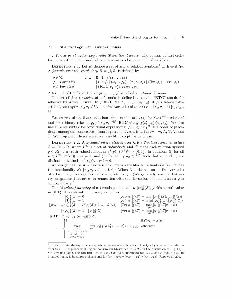
Fig. 11. A store in which u is shared; i.e., isn(u) = 1.
place of c is equivalent to using the value of c when ψp is evaluated in Sproto; i.e.,
for all Z, [[ψp[c←↩ τc,st | c ∈ C]]]S1
2 (Z) = [[ψp]]Sproto
2 (Z). However—and this is pre-cisely the drawback of using Eqn. (5) to obtain the µp,st—the steps of evaluating
[[ψp[c←↩ τc,st | c ∈ C]]]S1
2 (Z) mimic exactly those of evaluating [[ψp]]Sproto
2 (Z). Con-
sequently, when we pass to 3-valued logic, for all Z, [[ψp[c←↩ τc,st | c ∈ C]]]S#
1
3 (Z)
yields exactly the same value as [[ψp]]S#
proto
3 (Z) (i.e., as evaluating Eqn. (3)). Thus,although µp,st that satisfy Defn. 3.1 can be obtained automatically via Eqn. (5),this approach does not provide a satisfactory solution to the relation-maintenanceproblem.
Example 3.2. Eqn. (6) shows the defining formula for the instrumentation re-lation isn (“is-shared using n fields”),
isn(v)def
= ∃ v1, v2 : n(v1, v)∧n(v2, v)∧ v1 6=v2, (6)
which captures whether a memory cell is pointed to by two or more pointer fieldsof memory cells, e.g., see Fig. 11.
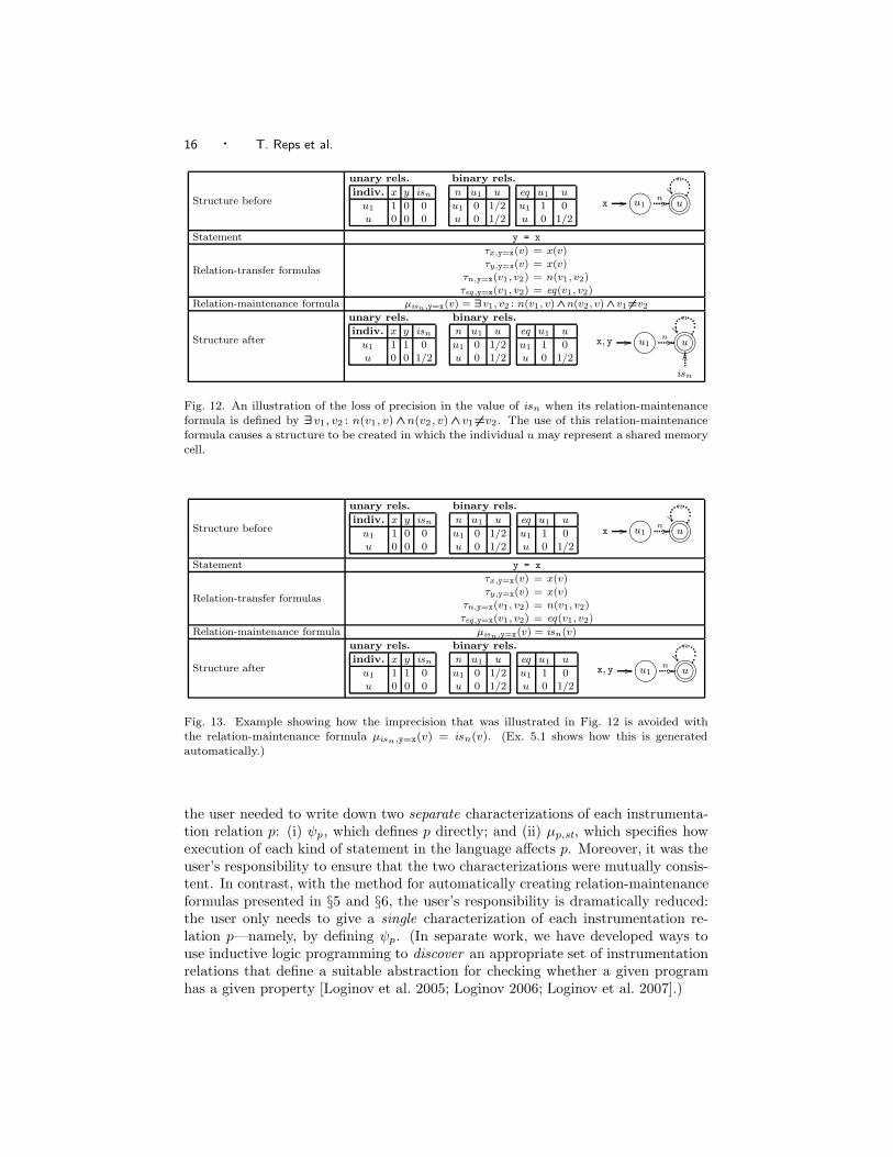
Fig. 12 illustrates how execution of the statement y = x causes the value of isn
to lose precision when its relation-maintenance formula is created according toEqn. (5). The initial 3-valued structure represents all singly-linked lists of length 2or more in which all memory cells are unshared. Because execution of y = x does notchange the value of core relation n, τn,y=x(v1, v2) is n(v1, v2), and hence the formulaµisn,y=x(v) created according to Eqn. (5) is ∃ v1, v2 : n(v1, v)∧n(v2, v)∧ v1 6=v2. Asshown in Fig. 12, the structure created using this maintenance formula is not asprecise as we would like. In particular, isn(u) = 1/2, which means that u canrepresent a shared cell. Thus, the final 3-valued structure also represents certaincyclic linked lists, such as
x, y // GFED@ABCu1n // GFED@ABCu2
n // GFED@ABCu3n // GFED@ABCu4
n // GFED@ABCu5ee
2
This sort of imprecision can usually be avoided by devising better relation-maintenance formulas. For instance, when µisn,y=x(v) is defined to be the formulaisn(v)—meaning that y = x does not change the value of isn(v)—the imprecisionillustrated in Fig. 12 is avoided (see Fig. 13). Hand-crafted relation-maintenanceformulas for a variety of instrumentation relations are given in [Sagiv et al. 2002;Lev-Ami and Sagiv 2000; TVLA ]; however, those formulas were created by ad hocmethods.
To sum up, prior to the work presented in this paper, the user needed to supplya formula µp,st for each instrumentation relation p and each statement st. In effect,
16 · T. Reps et al.
Structure before
unary rels. binary rels.
indiv. x y isn
u1 1 0 0u 0 0 0
n u1 u
u1 0 1/2u 0 1/2
eq u1 u
u1 1 0u 0 1/2
x // ?>=<89:;u1n //?>=<89:;/.-,()*+u
n
��
Statement y = x
Relation-transfer formulas
τx,y=x(v) = x(v)τy,y=x(v) = x(v)
τn,y=x(v1, v2) = n(v1, v2)τeq,y=x(v1, v2) = eq(v1, v2)
Relation-maintenance formula µisn,y=x(v) = ∃v1, v2 : n(v1, v) ∧n(v2, v) ∧v1 6=v2
Structure after
unary rels. binary rels.
indiv. x y isn
u1 1 1 0u 0 0 1/2
n u1 u
u1 0 1/2u 0 1/2
eq u1 u
u1 1 0u 0 1/2
x, y // ?>=<89:;u1n //?>=<89:;/.-,()*+u
n
��
isn
OO
Fig. 12. An illustration of the loss of precision in the value of isn when its relation-maintenanceformula is defined by ∃v1, v2 : n(v1, v) ∧n(v2, v) ∧v1 6=v2. The use of this relation-maintenanceformula causes a structure to be created in which the individual u may represent a shared memorycell.
Structure before
unary rels. binary rels.
indiv. x y isn
u1 1 0 0u 0 0 0
n u1 u
u1 0 1/2u 0 1/2
eq u1 u
u1 1 0u 0 1/2
x // ?>=<89:;u1n //?>=<89:;/.-,()*+u
n
��
Statement y = x
Relation-transfer formulas
τx,y=x(v) = x(v)τy,y=x(v) = x(v)
τn,y=x(v1, v2) = n(v1, v2)τeq,y=x(v1, v2) = eq(v1, v2)
Relation-maintenance formula µisn,y=x(v) = isn(v)
Structure after
unary rels. binary rels.
indiv. x y isn
u1 1 1 0u 0 0 0
n u1 u
u1 0 1/2u 0 1/2
eq u1 u
u1 1 0u 0 1/2
x, y // ?>=<89:;u1n //?>=<89:;/.-,()*+u
n
��
Fig. 13. Example showing how the imprecision that was illustrated in Fig. 12 is avoided withthe relation-maintenance formula µisn,y=x(v) = isn(v). (Ex. 5.1 shows how this is generatedautomatically.)
the user needed to write down two separate characterizations of each instrumenta-tion relation p: (i) ψp, which defines p directly; and (ii) µp,st, which specifies howexecution of each kind of statement in the language affects p. Moreover, it was theuser’s responsibility to ensure that the two characterizations were mutually consis-tent. In contrast, with the method for automatically creating relation-maintenanceformulas presented in §5 and §6, the user’s responsibility is dramatically reduced:the user only needs to give a single characterization of each instrumentation re-lation p—namely, by defining ψp. (In separate work, we have developed ways touse inductive logic programming to discover an appropriate set of instrumentationrelations that define a suitable abstraction for checking whether a given programhas a given property [Loginov et al. 2005; Loginov 2006; Loginov et al. 2007].)

Finite Differencing of Logical Formulas · 17
4. OUR APPROACH AT AN INFORMAL LEVEL
As illustrated by Ex. 3.2, relation-maintenance formulas that are defined by Eqn. (5)can yield imprecise answers. In essence, Eqn. (5) specifies that the new value ofinstrumentation relation p should be computed using its defining formula ψp, buttaking into account updates to any core relation c that occurs in ψp. Unfortunately,the approach of Eqn. (5) is equivalent to that of Eqn. (3): they both rely onrecomputing the value of instrumentation relation p based on its defining formulaψp. In the presence of abstraction, the indefinite value 1/2 for a core-relation tupleoften causes recomputed instrumentation-relation tuples to evaluate to 1/2, as well.For instance, as illustrated in Ex. 3.2, the dashed n edges incident on u in Fig. 12cause isn(u) to evaluate to 1/2.
As we saw in Fig. 13, such recomputation is not always necessary. The valuesof n—the only core relation that is used to define isn—cannot change as a resultof executing y = x; consequently, the values of instrumentation relation isn do notneed to change as a result of y = x. Moreover, as will become apparent shortly,even when the values of tuples in an instrumentation relation do need to change,they can often be maintained more precisely by means other than recomputation.
The framework of Sagiv et al. includes a mechanism for maintaining more precisevalues for core-relation tuples in abstract structures. Roughly speaking, the focusoperation is used to ensure that the core-relation tuples in the “vicinity” of an up-date have precise values during a structure transformation, although they may beset to 1/2 when abstraction is applied at the end of the transformation. (For moredetails about focus, see [Sagiv et al. 2002, §6.3].) Most programming languageshave the property that they perform only localized changes to core relations. As apractical matter, what this meant for the TVLA system—prior to our work—wasthat it was usually possible to create hand-crafted relation-maintenance formulasthat retain precision under most circumstances. However, prior to the adoption inTVLA of the techniques presented in §5 and §6 for creating relation-maintenanceformulas automatically, the task of crafting a good set of relation-maintenance for-mulas required substantial expertise, and remained a bit of “black art”.
Fig. 14 illustrates some of the issues; it addresses the problem of maintain-ing isn in response to the execution of the statement x→n = y, assuming thatx→n = NULL. The statement changes relation n: it adds a new n edge from theindividual pointed to by x to that pointed to by y. Thus, the relation-maintenanceformula for isn is nontrivial. However, by noting that isn can only change in a smallpart of the structure (the “vicinity” of the update), one can specify the followingincremental relation-maintenance formula:
µisn,x→n=y(v) = isn(v)∨(y(v)∧ ∃ v1 : n(v1, v)). (7)
Eqn. (7) reuses the stored value of isn for all individuals, except the one that ispointed to by y. For that individual, it checks whether it has an incoming n edgeprior to the update. In Fig. 14 it does not, and the value of isn remains 0 for allindividuals.
In our first attempt to automate the process of computing incremental relation-maintenance formulas for first-order logic, we defined the finite-differencing schemeshown in Fig. 15. In this scheme, ∆st[ϕ] captures the change to ϕ’s value. With

18 · T. Reps et al.
Structure before
unary rels. binary rels.
indiv. x y isn
u1 1 0 0u2 0 1 0u 0 0 0
n u1 u2 u
u1 0 0 0u2 0 0 1/2u 0 0 1/2
eq u1 u2 u
u1 1 0 0u2 0 1 0u 0 0 1/2
x // ?>=<89:;u1
y // ?>=<89:;u2n //?>=<89:;/.-,()*+u
n
��
Statement x→n = y (assuming x→n = NULL)
Relation-transfer formulas
τx,x→n=y(v) = x(v)τy,x→n=y(v) = y(v)
τn,x→n=y(v1, v2) = n(v1, v2) ∨(x(v1) ∧y(v2))τeq,x→n=y(v1, v2) = eq(v1, v2)
Relation-maintenance formula µisn,x→n=y(v) = isn(v) ∨(y(v) ∧∃v1 : n(v1, v))
Structure after
unary rels. binary rels.
indiv. x y isn
u1 1 0 0u2 0 1 0u 0 0 0
n u1 u2 u
u1 0 1 0u2 0 0 1/2u 0 0 1/2
eq u1 u2 u
u1 1 0 0u2 0 1 0u 0 0 1/2
x // ?>=<89:;u1
��y // ?>=<89:;u2
n //?>=<89:;/.-,()*+u
n
��
Fig. 14. Example of a nontrivial relation-maintenance formula for relation isn.
ϕ ∆st[ϕ]
1 0
0 0
p(w1, . . . , wk), p ∈ C (τp,st ⊕p){w1, . . . , wk}
p(w1, . . . , wk), p ∈ I ∆st[ψp]{w1, . . . , wk}
ϕ1 ⊕ϕ2 ∆st[ϕ1] ⊕∆st[ϕ2]
ϕ1 ∧ϕ2 (∆st[ϕ1]∧ϕ2) ⊕(ϕ1 ∧∆st[ϕ2]) ⊕(∆st[ϕ1] ∧∆st[ϕ2])
∀v : ϕ1 (∀v : ϕ1) ? (∃v : ∆st[ϕ1]) : (∀v : ϕ1 ⊕∆st[ϕ1])
Fig. 15. A finite-differencing scheme for first-order formulas, based on exclusive-or (⊕).
Fig. 15, the maintenance formula for instrumentation relation p is
µp,stdef
= p⊕∆st[ψp], (8)
where ⊕ denotes exclusive-or. However, in 3-valued logic, we have 1/2⊕V = 1/2,regardless of whether V is 0, 1, or 1/2. Consequently, Eqn. (8) has the unfortunateproperty that if p(u) = 1/2, then µp,st evaluates to 1/2 on u, and p(u) becomes“pinned” to the indefinite value 1/2; it will have the value 1/2 in all successor
structures S#2 , in all successors of S#
2 , and so on. With Eqn. (8), p(u) can neverreacquire a definite value.
This led us to consider a scheme that separates the negative change to a formula’svalue from the positive change:
µp,st = p ? ¬∆−st[ψp] : ∆+
st[ψp], (9)
where finite-differencing operators ∆−st[·] and ∆+
st[·] capture the negative and positivechanges, respectively. (These operators are discussed in detail in §5 and §6.) In thisapproach to the relation-maintenance problem, the two finite-differencing operatorscharacterize the tuples of a relation that are subtracted and added in response to astructure transformation.
Because they have the form p ? ¬∆−st[ψp] : ∆+
st[ψp], the maintenance formulascreated using Eqn. (9) do not suffer from the problem exhibited by the mainte-nance formulas created using Eqn. (8) (discussed above). The use of if-then-elseallows p(u) to reacquire a definite value after it has been set to 1/2: when p(u)

Finite Differencing of Logical Formulas · 19
is 1/2, µp,st evaluates to a definite value on u if [[∆−st[ψp(v)]]]
S#
3 ([v 7→ u]) is 1 and
[[∆+st[ψp(v)]]]
S#
3 ([v 7→ u]) is 0, or vice versa.
Limitations. The finite-differencing technique that we present in this paper isapplicable to any method in which systems are described as evolving (2-valued or3-valued) logical structures. However, it is important to note some limitations of theapproach. First, it relies on a first-order encoding of all properties. In particular,the finite-differencing technique includes no explicit handling of numerical proper-ties; we expect those to be modeled implicitly by other relations, such as the binaryrelation dle (see §2.2). It may be possible to combine numerical finite differencing[Goldstine 1977] with our approach, thus creating a finite-differencing techniquethat is prepared to handle numerical properties explicitly. Second, for maintainingtransitive-closure (reachability) relations, the finite-differencing technique is effec-tive only when transitive-closure relations can be updated using first-order formulas.§6 describes in detail the extent to which our approach can be used to maintaintransitive-closure relations.
5. RELATION MAINTENANCE FOR 2-VALUED (AND 3-VALUED) FIRST-ORDERLOGIC VIA FINITE DIFFERENCING
This section presents an algorithm for creating relation-maintenance formulas thatis based on finite differencing. The discussion will be couched primarily in termsof 2-valued logic; however, by the Embedding Theorem (Theorem 2.6, [Sagiv et al.2002, Theorem 4.9]), the relation-maintenance formulas that we derive providesound results when interpreted in 3-valued logic. In 3-valued logic, as demonstratedin Fig. 13 (and discussed further in Ex. 5.1), the resulting formula can lead to astrictly more precise result than merely reevaluating an instrumentation relation’sdefining formula.
Our algorithm for creating a relation-maintenance formula µp,st, for p ∈ I, usesan incremental-computation strategy: µp,st is defined in terms of the stored (pre-state) value of p, along with two finite-differencing operators, denoted by ∆−
st[·] and∆+
st[·]. The finite-differencing operators capture the negative and positive changes,respectively, that execution of structure transformer st induces in an instrumenta-tion relation’s value. The formula µp,st is defined as follows:
µp,st = p ? ¬∆−st[ψp] : ∆+
st[ψp]. (10)
Maintenance formula µp,st specifies the new value of p (i.e., its value in S2, in the
case of a 2-valued structure, or S#2 , in the case of a 3-valued structure) in terms of
the old values of p, ∆−st[ψp], and ∆+
st[ψp] (i.e., their values in S1 or S#1 ). Eqn. (10)
states that if p’s old value is 1, then its new value is 1 unless there is a negativechange; if p’s old value is 0, then its new value is 1 if there is a positive change.
Fig. 16 depicts how the static-analysis engine evaluates ∆−st[ψp] and ∆+
st[ψp] in
S#1 and combines these values with the old value p to obtain the desired new valuep′′. The operators ∆−
st[·] and ∆+st[·] are defined recursively, as shown in Fig. 17.
The definitions in Fig. 17 make use of the operator Fst[ϕ] (standing for “Future”),defined as follows:
Fst[ϕ]def
= ϕ ? ¬∆−st[ϕ] : ∆+
st[ϕ]. (11)

20 · T. Reps et al.
evaluate�p
retrievestoredvalue
execute statement st
p p′′ b p′
∆–[�p]st
∆+[�p]st
evaluate∆+[�p]stevaluate
∆–[�p]st
p ? ¬∆–[�p] : ∆+[�p]st st
S1# Sproto
#
Fig. 16. How to maintain the value of ψp in 3-valued logic in response to changes in the values ofcore relations caused by the execution of structure transformer st.
Thus, maintenance formula µp,st can also be expressed as µp,st = Fst[p].Formula (11) and Fig. 17 define a syntax-directed translation scheme that can be
implemented via a recursive walk over a formula ϕ. The operators ∆−st[·] and ∆+
st[·]are mutually recursive. For instance, ∆+
st[¬ϕ1] = ∆−st[ϕ1] and ∆−
st[¬ϕ1] = ∆+st[ϕ1].
Moreover, each occurrence of Fst[ϕi] contains additional occurrences of ∆−st[ϕi] and
∆+st[ϕi].Note how ∆−
st[·] and ∆+st[·] for ϕ1 ∨ϕ2 and ϕ1 ∧ϕ2 exhibit the “convolution”
pattern characteristic of differentiation, finite differencing, and divided differencing.Continuing the analogy with differentiation, it helps to bear in mind that the
“independent variables” are the core relations—which are being changed by theτc,st formulas; the dependent variable is the value of ϕ. A formal justification ofFig. 17 is stated later (Theorem 5.3 and Cor. 5.4); here we merely explain informallya few of the cases from Fig. 17:
∆+st[1] = 0, ∆−
st[1] = 0. The value of atomic formula 1 does not depend on anycore relations; hence its value is unaffected by changes in them.
∆−st[ϕ1 ∧ϕ2] = (∆−
st[ϕ1] ∧ϕ2)∨(ϕ1 ∧ ∆−st[ϕ2]). Tuples of individuals removed
from ϕ1 ∧ϕ2 are either tuples of individuals removed from ϕ1 for which ϕ2 alsoholds (i.e., (∆−
st[ϕ1] ∧ϕ2)), or they are tuples of individuals removed from ϕ2 forwhich ϕ1 also holds, (i.e., (ϕ1 ∧ ∆−
st[ϕ2]).
∆+st[∃ v : ϕ1] = (∃ v : ∆+
st[ϕ1])∧¬(∃ v : ϕ1). For ∃ v : ϕ1 to change value from 0to 1, there must be at least one individual for which ϕ1 changes value from 0 to 1(i.e., ∃ v : ∆+
st[ϕ1] holds), and ∃ v : ϕ1 must not already hold (i.e., ¬(∃ v : ϕ1) holds).
∆+st[p(w1, . . . , wk)] = (∃ v : ∆+
st[ϕ1])∧¬p, if p ∈ I and ψp ≡ ∃ v : ϕ1. This case issimilar to the previous one, except that the term to ensure that ∃ v : ϕ1 doesnot already hold (i.e., ¬(∃ v : ϕ1)) is replaced by the formula ¬p. Thus, when(∃ v : ∆+
st[ϕ1])∧ ¬p is evaluated, the stored value of ∃ v : ϕ1, i.e., p, will be usedinstead of the value obtained by reevaluating ∃ v : ϕ1.
∆+st[p(w1, . . . , wk)] = ∆+
st[ψp{w1, . . . , wk}], if p ∈ I and ψp 6≡ ∃ v : ϕ1. To charac-terize the positive changes to p, apply ∆+
st to p’s defining formula ψp.
One special case is also worth noting: ∆+st[v1 =v2] = 0 and ∆−
st[v1 =v2] = 0 becausethe value of the atomic formula (v1 =v2) (shorthand for eq(v1, v2)) does not dependon any core relations; hence, its value is unaffected by changes in them.5
5We avoid issues that could arise due to changes in a structure’s universe of individuals by modelingstorage allocation and deallocation via a free-storage list. We describe our solution in more detailat the end of this section.

Fin
iteD
ifferen
cing
ofLogica
lForm
ula
s·
21
ϕ ∆+st[ϕ] ∆−
st[ϕ]
1 0 00 0 0p(w1, . . . , wk),p ∈ C, and τp,st
is of the formp ? ¬δ−p,st : δ+p,st
(δ+p,st ∧¬p){w1, . . . , wk} (δ−p,st ∧ p){w1, . . . , wk}
p(w1, . . . , wk),p ∈ C, and τp,st
is of the formp∨ δp,st orδp,st ∨ p
(δp,st ∧¬p){w1, . . . , wk} 0
p(w1, . . . , wk),p ∈ C, and τp,st
is of the formp∧ δp,st orδp,st ∧ p
0 (¬δp,st ∧ p){w1, . . . , wk}
p(w1, . . . , wk),p ∈ C, but τp,st
is not of theabove forms
(τp,st ∧ ¬p){w1, . . . , wk} (p∧¬τp,st){w1, . . . , wk}
p(w1, . . . , wk),p ∈ I
((∃ v : ∆+st[ϕ1])∧ ¬p){w1, . . . , wk} ifψp ≡ ∃ v : ϕ1
∆+st[ψp]{w1, . . . , wk} otherwise
((∃ v : ∆−st[ϕ1])∧ p){w1, . . . , wk} ifψp ≡ ∀ v : ϕ1
∆−st[ψp]{w1, . . . , wk} otherwise
¬ϕ1 ∆−st[ϕ1] ∆+
st[ϕ1]
ϕ1 ∨ϕ2 (∆+st[ϕ1] ∧¬ϕ2)∨(¬ϕ1 ∧ ∆+
st[ϕ2]) (∆−st[ϕ1] ∧¬Fst[ϕ2])∨(¬Fst[ϕ1] ∧∆−
st[ϕ2])
ϕ1 ∧ϕ2 (∆+st[ϕ1] ∧Fst[ϕ2])∨(Fst[ϕ1] ∧ ∆+
st[ϕ2]) (∆−st[ϕ1] ∧ϕ2)∨(ϕ1 ∧ ∆−
st[ϕ2])
∃ v : ϕ1 (∃ v : ∆+st[ϕ1])∧ ¬(∃ v : ϕ1) (∃ v : ∆−
st[ϕ1])∧¬(∃ v : Fst[ϕ1])
∀ v : ϕ1 (∃ v : ∆+st[ϕ1])∧(∀ v : Fst[ϕ1]) (∃ v : ∆−
st[ϕ1])∧(∀ v : ϕ1)
Fig. 17. Finite-difference formulas for first-order formulas.

22 · T. Reps et al.
∆+st [isn(v)] =
(
∃v1, v2 :
(
(∆+st [n(v1, v)] ∧Fst[n(v2, v)])
∨ (Fst[n(v1, v)] ∧∆+st [n(v2, v)])
)
∧v1 6=v2
)
∧¬isn(v)
∆−
st [isn(v)] =
(
∃v1, v2 :
(
(∆−
st [n(v1, v)] ∧n(v2, v))
∨ (n(v1, v) ∧∆−
st [n(v2, v)])
)
∧v1 6=v2
)
∧
¬
∃v1, v2 :
(n(v1, v) ∧n(v2, v) ∧v1 6=v2)
? ¬
((
(∆−
st [n(v1, v)] ∧n(v2, v))
∨ (n(v1, v) ∧∆−
st [n(v2, v)])
)
∧v1 6=v2
)
:
(
(∆+st [n(v1, v)] ∧Fst[n(v2, v)])
∨ (Fst[n(v1, v)] ∧∆+st [n(v2, v)])
)
∧v1 6=v2
Fig. 18. Finite-difference formulas for the instrumentation relation isn(v).
Example 5.1. Consider the instrumentation relation isn (“is-shared using n
fields”), defined in Eqn. (6). Fig. 18 shows the formulas obtained for ∆+st[isn(v)]
and ∆−st[isn(v)].
For a particular statement, the formulas in Fig. 18 can usually be simplified.For instance, for y = x, the relation-transfer formula τn,y=x(v1, v2) is n(v1, v2); seeFig. 12. Thus, by Fig. 17, the formulas for ∆−
y=x[n(v1, v)] and ∆+y=x[n(v1, v)] are
both n(v1, v)∧¬n(v1, v), which simplifies to 0. (In our implementation, sim-plifications are performed greedily at formula-construction time; e.g., the con-structor for ∧ rewrites 0∧ p to 0, 1∧ p to p, p∧¬p to 0, etc.) The formulasin Fig. 18 simplify to ∆+
y=x[isn(v)] = 0 and ∆−y=x[isn(v)] = 0. Consequently,
µisn,y=x(v) = Fy=x[isn(v)] = isn(v) ? ¬0 : 0 = isn(v). As shown in Fig. 13, thisdefinition of µisn,y=x(v) avoids the imprecision that was illustrated in Ex. 3.2. 2
Correctness of the Relation-Maintenance Scheme
The correctness of the finite-differencing scheme given above is established with thehelp of the following lemma:
Lemma 5.2. For every formula ϕ, ϕ1, ϕ2 and structure transformer st, the fol-lowing properties hold:6
(i). ∆+st[ϕ]
meta
⇐⇒ Fst[ϕ] ∧ ¬ϕ
(ii). ∆−st[ϕ]
meta
⇐⇒ ϕ∧¬Fst[ϕ]
(iii). (a). Fst[¬ϕ1]meta
⇐⇒ ¬Fst[ϕ1]
(b). Fst[ϕ1 ∨ϕ2]meta
⇐⇒ Fst[ϕ1] ∨Fst[ϕ2]
(c). Fst[ϕ1 ∧ϕ2]meta
⇐⇒ Fst[ϕ1] ∧Fst[ϕ2]
(d). Fst[∃ v : ϕ1]meta
⇐⇒ ∃ v : Fst[ϕ1]
(e). Fst[∀ v : ϕ1]meta
⇐⇒ ∀ v : Fst[ϕ1]
Proof. See App. A.
Lemma 5.2 shows that for structures in S2, ∆+st[ϕ] specifies the tuples that are not
in the relation defined by ϕ, but need to be added in response to the execution of st,
6To simplify the presentation, we use lhsmeta⇐⇒rhs and lhs
meta=⇒rhs as shorthands for [[lhs]]S2 (Z) =
[[rhs]]S2 (Z) and [[lhs]]S2 (Z) ≤ [[rhs]]S2 (Z), respectively, for any S ∈ S2 and assignment Z that iscomplete for lhs and rhs.

Finite Differencing of Logical Formulas · 23
ϕ Fst[ϕ]
1 1
0 0
p(w1, . . . , wk), p ∈ C τp,st{w1, . . . , wk}
p(w1, . . . , wk), p ∈ I p(w1, . . . , wk) ? ¬∆−
st [p(w1, . . . , wk)] : ∆+st [p(w1, . . . , wk)]
¬ϕ1 ¬Fst[ϕ1]
ϕ1 ∨ϕ2 Fst[ϕ1] ∨ Fst[ϕ2]
ϕ1 ∧ϕ2 Fst[ϕ1] ∧ Fst[ϕ2]
∃ v : ϕ1 ∃ v : Fst[ϕ1]
∀ v : ϕ1 ∀ v : Fst[ϕ1]
Fig. 19. Optimized formulas for the operator Fst[ϕ].
and that ∆−st[ϕ] specifies the tuples that are in the relation defined by ϕ that need to
be removed. Lemma 5.2 is used in the proof of the following theorem, which ensuresthe correctness of the finite-differencing transformation given in Fig. 17, as well asthe finite-differencing-based scheme for relation maintenance given in Eqn. (10):
Theorem 5.3. Let S1 be a structure in S2, and let Sproto be the proto-structure obtained from S1 using structure transformer st. Let S2 be the struc-ture obtained by using Sproto as the first approximation to S2 and then fill-ing in instrumentation relations in a topological ordering of the dependencesamong them: for each arity-k relation p ∈ I, ιS2(p) is obtained by evaluating[[ψp(v1, . . . , vk)]]S2
2 ([v1 7→ u′1, . . . , vk 7→ u′k]) for all tuples (u′1, . . . , u′k) ∈ (US2)k.
Then for every formula ϕ(v1, . . . , vk) and complete assignment Z for ϕ(v1, . . . , vk),[[Fst[ϕ(v1, . . . , vk)]]]S1
2 (Z) = [[ϕ(v1, . . . , vk)]]S2
2 (Z).
Proof. See App. A.
For structures in S3, the soundness of the finite-differencing transformation givenin Fig. 17, as well as the finite-differencing-based scheme for relation maintenancegiven in Eqn. (10), follows from Theorem 5.3 by the Embedding Theorem (Theo-rem 2.6):
Corollary 5.4. Let S1, S2 ∈ S2 be defined as in Theorem 5.3. Let S#1 ∈
S3 be such that f : US1 → US#1 embeds S1 in S#
1 , i.e., S1 vf S#1 . Then
for every formula ϕ(v1, . . . , vk) and complete assignment Z for ϕ(v1, . . . , vk),
[[Fst[ϕ(v1, . . . , vk)]]]S#
1
3 (f ◦ Z) w [[ϕ(v1, . . . , vk)]]S2
2 (Z). 2
Optimized Formulas for Fst[ϕ]
For a non-atomic formula ϕ, the operator Fst[ϕ] defined in Formula (11) intro-duces a copy of ϕ, because it has no way, in general, to refer to a relation thatholds the stored value of ϕ. The reevaluation of ϕ inherent in the version of Fst[·]
from Formula (11) (i.e., Fst[ϕ]def
= ϕ ? . . . : . . .) may cause a substantial loss ofprecision. One way to retain higher precision is to propagate Fst[·] into the subfor-mulas of ϕ, down to the level of atomic formulas—either core-relation symbols orinstrumentation-relation symbols—as shown in Fig. 19.
Suppose that ϕ′ is the result of Fst[ϕ] by the method of Fig. 19. An evaluationof ϕ′ will evaluate (copies of) the operators of ϕ, down to the level of each atomic

24 · T. Reps et al.
subformula p(w1, . . . , wk) in ϕ. At that level, if p ∈ I, Fst[·] will have introducedan occurrence of p in ϕ′:
Fst[p(w1, . . . , wk)]def
= p(w1, . . . , wk) ? ¬∆−st[p(w1, . . . , wk)] : ∆+
st[p(w1, . . . , wk)].(12)
The occurrence of p in the test refers to the stored (“pre-state”) value ofinstrumentation-relation p; consequently, the stored tuples of relation p will beused when evaluating ϕ′.
Note that ∆+st[p] and ∆−
st[p] in Formula (12) dispatch according to the case forp ∈ I in Fig. 17. In particular, because Fst[·] occurs in four of the eight cases for∆+
st[·] and ∆−st[·] in Fig. 17—i.e., for ∨, ∧, ∃, and ∀—the optimized Fst[·] is invoked
recursively on various subterms of ψp.The correctness of the version of Fst[·] defined in Fig. 19 follows from Lemma 5.2.The method described above also usually produces smaller instrumentation-
relation maintenance formulas, and hence creates abstract transformers that gen-erally can be evaluated more quickly. This technique is incorporated into our im-plementation.
Complexity of the Relation-Maintenance Scheme
There are at most three operations that can be applied to each subformula ϕ consid-ered during the method for creating a relation-maintenance formula: Fst[ϕ], ∆−
st[ϕ],and ∆+
st[ϕ]. Duplicate work can be avoided be performing function caching (alsoknown as memoization [Michie 1968]). Moreover, for each of the possible operator-node kinds for ϕ’s outermost operator, each of the operations Fst[ϕ], ∆−
st[ϕ], and∆+
st[ϕ] introduces a constant number of operator nodes into the answer formula(together with the results of additional calls on Fst[ϕi], ∆−
st[ϕi], and ∆+st[ϕi] for
various subformula(s) ϕi of ϕ). We will assume that the algorithm (i) uses a DAGrepresentation of the output formula (so that subformulas are shared in the answerformula), (ii) memoizes calls on Fst[ϕ], ∆−
st[ϕ], and ∆+st[ϕ] (thereby possibly creating
shared subformulas in the answer formula), and (iii) the hashed-lookup operationused during memoization takes unit time per lookup. Under these assumptions,for an instrumentation relation defined by formula ψ, the overall cost of creating arelation-maintenance formula via our finite-differencing scheme is linear in the sizeof the DAG that represents ψ in core normal form (see §3).
Discussion
Earlier in the paper we touted the advantages of being able to apply related 2-valuedand 3-valued interpretation functions to a single formula—which, in essence, usesoverloading to define two related meaning functions. Thus, it may seem somewhatinconsistent for us to address the problem of maintaining instrumentation relationsby an approach that involves explicit transformations of formulas rather than byan approach based on overloading. (In unpublished work, we have studied suchan approach—e.g., interpreting instrumentation predicate p’s defining formula ψp
with respect to both the pre-state structure S1 and a specification of the differencesbetween the core predicates of S1 and those of Sproto.) The reason that we usea transformation-based approach is that it gives us an opportunity to simplifythe resulting formulas (either on the fly, or in a post-processing phase after finite

Finite Differencing of Logical Formulas · 25
differencing).In the context of evaluation in 3-valued logic, simplification is important be-
cause even formulas that are tautologies in 2-valued logic may evaluate to 1/2 in3-valued logic. For instance, p∨¬p yields 1/2 when p has the value 1/2, evenwhen p is a nullary relation symbol. The finite-differencing transformation thatwe implemented uses a formula-minimization procedure for 3-valued logic that wedeveloped [Reps et al. 2002]. The minimization procedure applies to propositionallogic; for propositional logic, it is guaranteed to return an answer that capturesthe formula’s “supervaluational meaning” [van Fraassen 1966]. This procedure isused as a subroutine in a heuristic method for minimizing first-order formulas; themethod works on a formula bottom-up, applying the propositional minimizer to thebody of each non-propositional operator (i.e., each quantifier or transitive-closureoperator).
A relation-maintenance formula that has been simplified in this way can some-times yield a definite value in situations where the evaluation of the unsimplifiedrelation-maintenance formula—or, equivalently, an overloaded evaluation of the re-lation’s defining formula—yields 1/2. (For instance, minimizing p∨¬p yields 1,which evaluates to 1 even when p has the value 1/2.) Consequently, the formula-transformation approach to the relation-maintenance problem leads to more precisestatic-analysis algorithms.
Malloc and Free
In [Sagiv et al. 2002], the modeling of storage-allocation/deallocation operations iscarried out with a two-stage structure transformer, the first stage of which changesthe number of individuals in the structure. This creates some problems for thefinite-differencing approach in establishing appropriate, mutually consistent valuesfor relation tuples that involve the newly allocated individual. Such relation valuesare needed for the second stage, in which relation-transfer formulas for core relationsand relation-maintenance formulas for instrumentation relations are applied in theusual fashion, using Eqns. (2) and (4).
However, there is a simple way to sidestep this problem, which is to model thefree-storage list explicitly, making the following substructure part of every 3-valuedstructure:
freelist // GFED@ABCu1n // ?>=<89:;/.-,()*+u
n
��(13)
A malloc is modeled by advancing the pointer freelist into the list, and returningthe memory cell that it formerly pointed to. A free is modeled by inserting, atthe head of freelist’s list, the cell being deallocated. This approach models limitson available storage naturally, while the introduction of one integrity constraintenables it to model unbounded storage.7
It is true that the use of structure (13) to model storage-allocation/deallocationoperations also causes the number of individuals in a 3-valued structure to change;
7Instead of a free-storage list, one could use a (bounded or unbounded) set of memory locationsto model storage allocation and deallocation. In that approach, instead of reachability from thepointer freelist, a core unary relation would mark free cells, thus distinguishing them fromallocated cells that have been leaked.

26 · T. Reps et al.
p IntendedMeaning ψp
tn(v1, v2) Is v2 reachable from v1 along n fields? n∗(v1, v2)rn,z(v) Is v reachable from pointer variable z along n fields? ∃v1 : z(v1) ∧ tn(v1, v)cn(v) Is v on a directed cycle of n fields? ∃v1 : n(v1, v) ∧ tn(v, v1)
Fig. 20. Defining formulas of some instrumentation relations that depend on RTC. (Recall thatn∗(v1, v2) is a shorthand for (RTC v′1, v
′
2 : n(v′1, v′
2))(v1, v2).)
however, because the new individual is materialized using the usual mechanismsfrom [Sagiv et al. 2002] (namely, the focus and coerce operations), values for relationtuples that involve the newly materialized individual will always have safe, mutuallyconsistent values.
6. MAINTENANCE FORMULAS FOR REACHABILITY AND TRANSITIVE CLO-SURE
Several instrumentation relations that depend on RTC are shown in Fig. 20. Un-fortunately, finding a good way to maintain instrumentation relations defined usingRTC is challenging because the evaluation of a formula that uses the RTC op-erator in a 3-valued structure generally produces many tuples with the value 1/2.This happens because in an abstracted binary relation, tuples (“edges”) that involvesummary individuals often have the value 1/2. (For instance, see the dashed nedges incident on u in structure (13).) Because the semantics of a tuple (u1, u2)computed via RTC is defined to be the “max over all paths P from u1 to u2 ofthe minimum value of an edge along P” (see Defns. 2.2 and 2.4), the presence ofindefinite edge-tuples often causes the path-tuple computed for a pair (u1, u2) tohave the value 1/2. Moreover, it is not known, in general, whether it is possibleto write a first-order formula (i.e., without using a transitive-closure operator) thatspecifies how to maintain the closure of a directed graph in response to edge in-sertions and deletions. Thus, our strategy has been to investigate special cases forclasses of instrumentation relations for which first-order maintenance formulas doexist. Whenever these do not apply, the system falls back on safe maintenanceformulas (which themselves use RTC).
In this section, we confine ourselves to important special cases for the main-tenance of instrumentation relations specified via the RTC of a binary formulaϕ1(v1, v2). In §6.1, we consider the case in which ϕ1(v1, v2) defines a directedacyclic graph. In §6.2, we consider the case in which ϕ1(v1, v2) defines a tree-shaped graph. Finally, in §6.3, we consider the case in which ϕ1(v1, v2) defines adeterministic graph—i.e., a possibly-cyclic graph, in which every node has outde-gree at most one (this class of graphs corresponds to possibly-cyclic linked lists).This collection of techniques allows us to handle most common data structures,such as lists (singly- and doubly-linked; cyclic and acyclic) and trees. The precisionof all of these techniques is due to the fact that maintenance of RTC after unit-size changes (single-edge additions or deletions)8 is performed via first-order logicalformulas only. However, maintaining RTC of an arbitrary directed graph, as wellas maintaining RTC of restricted classes of graphs with arbitrary-size changes, is
8These techniques can be extended to handle bounded-size addition and deletion sets.

Finite Differencing of Logical Formulas · 27
not known to be first-order expressible. In such cases, our algorithm returns a for-mula that uses the RTC operator; the evaluation of such a formula may yield moreindefinite answers than necessary.
To specify that the maintenance of binary relation p(v1, v2) defined as the RTC ofbinary formula ϕ1(v1, v2) should rely on one of the special cases, the user annotatesformula ϕ1 with attributes. To state that ϕ1(v1, v2) defines a directed acyclicgraph, the user gives ϕ1 attribute “acyclic”; to state that ϕ1(v1, v2) defines a tree-shaped graph, the user gives ϕ1 attribute “tree”; to state that ϕ1(v1, v2) definesa deterministic graph, the user gives ϕ1 attribute “function”. See Fig. 10 for theintended meanings of these attributes.
The analysis uses the attributes to generate integrity constraints to be enforced bythe sharpening operation coerce (see §2.2.2). For instance, when relation p(v1, v2)is defined as the RTC of formula ϕ1(v1, v2) that is annotated with the attribute“acyclic”, the analysis generates the following two constraints:
∀ v1, v2 : p(v1, v2)∧ p(v2, v1) ⇒ v1 = v2
∀ v1, v2 : p(v1, v2)∧ v1 6= v2 ⇒ ¬p(v2, v1).
When ϕ1(v1, v2) is annotated with the attribute “tree”, the analysis generates theabove acyclicity constraints, together with constraints that ensure that ϕ1(v1, v2)is an inverse partial function.
Whenever coerce determines that a constraint is (possibly) not satisfied after theapplication of a transformer, a warning is generated.
6.1 Transitive-Closure Maintenance in Directed Acyclic Graphs
Consider a binary instrumentation relation p, defined by ψp(v1, v2) ≡(RTC v′1, v
′2 : ϕ1)(v1, v2). If the graph defined by ϕ1 is acyclic, it is possible to
give a first-order formula that maintains p after the addition or deletion of a singleϕ1-edge. The method we use is a minor modification of a method for maintainingnon-reflexive transitive closure in a directed acyclic graph, due to Dong and Su[2000].
In the case of an insertion of a single ϕ1-edge, the maintenance formula is
Fst[p](v1, v2) = p(v1, v2)∨(∃ v′1, v′2 : p(v1, v
′1)∧∆+
st[ϕ1](v′1, v
′2)∧ p(v′2, v2)). (14)
The new value of p contains the old tuples of p, as well as those that representtwo old paths (i.e., p(v1, v
′1) and p(v′2, v2)) connected with the new ϕ1-edge (i.e.,
∆+st[ϕ1](v
′1, v
′2)).
The maintenance formula to handle the deletion of a single ϕ1-edge is a bit morecomplicated. We first identify the tuples of p that represent paths that might relyon the edge to be deleted, and thus may need to be removed from p (S stands forsuspicious):
S[p, ϕ1](v1, v2) = ∃ v′1, v′2 : p(v1, v
′1)∧∆−
st[ϕ1](v′1, v
′2)∧ p(v′2, v2).
We next collect a set of p-tuples that definitely remain in p (T stands for trusted):
T [p, ϕ1](v1, v2) = (p(v1, v2)∧ ¬S[p, ϕ1](v1, v2))∨Fst[ϕ1](v1, v2). (15)
Finally, the maintenance formula for p for a single ϕ1-edge deletion is
Fst[p](v1, v2) = ∃ v′1, v′2 : T [p, ϕ1](v1, v
′1)∧T [p, ϕ1](v
′1, v
′2)∧T [p, ϕ1](v
′2, v2). (16)
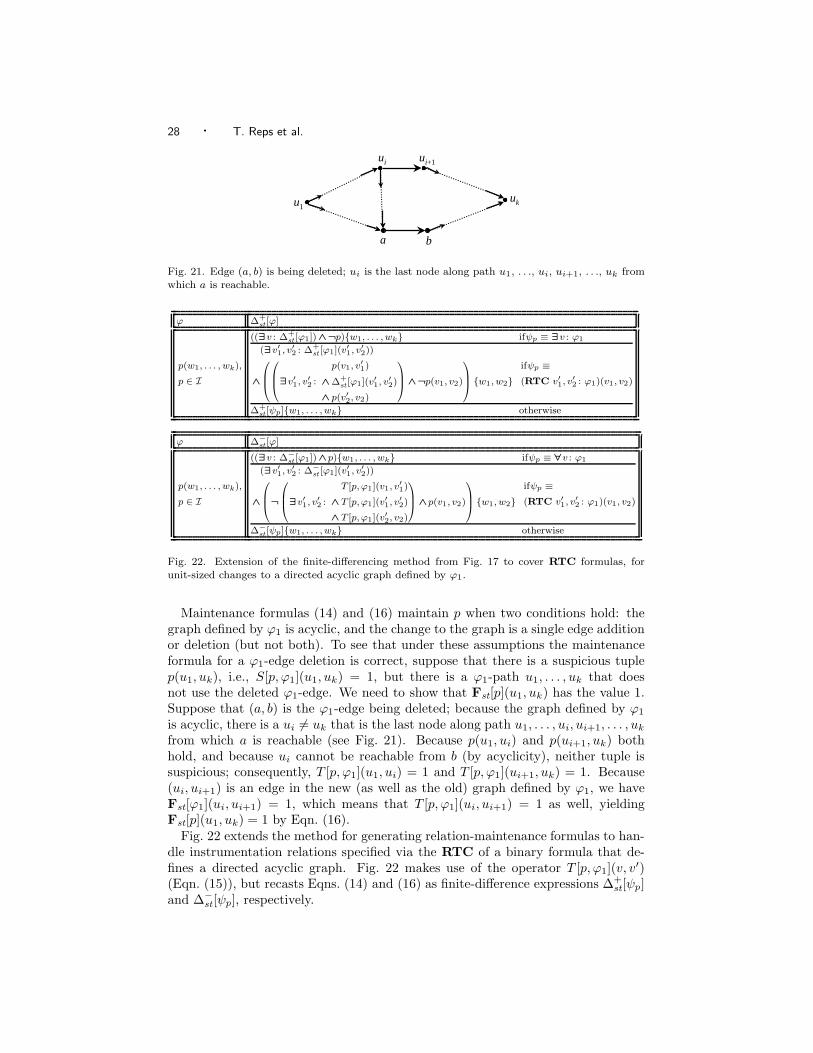
28 · T. Reps et al.
u1
ba
ui ui+1
uk
Fig. 21. Edge (a, b) is being deleted; ui is the last node along path u1, . . ., ui, ui+1, . . ., uk fromwhich a is reachable.
ϕ ∆+st [ϕ]
p(w1, . . . , wk),
p ∈ I
((∃v : ∆+st [ϕ1]) ∧¬p){w1, . . . , wk} ifψp ≡ ∃v : ϕ1
(∃v′1, v′
2 : ∆+st [ϕ1](v
′
1, v′
2))
∧
∃v′1, v
′
2 :
p(v1, v′
1)
∧ ∆+st [ϕ1](v
′
1, v′
2)
∧ p(v′2, v2)
∧¬p(v1, v2)
{w1, w2}
ifψp ≡
(RTC v′1, v′
2 : ϕ1)(v1, v2)
∆+st [ψp]{w1, . . . , wk} otherwise
ϕ ∆−
st [ϕ]
p(w1, . . . , wk),
p ∈ I
((∃v : ∆−
st [ϕ1]) ∧p){w1, . . . , wk} ifψp ≡ ∀v : ϕ1
(∃v′1, v′
2 : ∆−
st [ϕ1](v′
1, v′
2))
∧
¬
∃v′1, v
′
2 :
T [p,ϕ1](v1, v′
1)
∧ T [p,ϕ1](v′1, v′
2)
∧ T [p,ϕ1](v′2, v2)
∧p(v1, v2)
{w1, w2}
ifψp ≡
(RTC v′1, v′
2 : ϕ1)(v1, v2)
∆−
st [ψp]{w1, . . . , wk} otherwise
Fig. 22. Extension of the finite-differencing method from Fig. 17 to cover RTC formulas, forunit-sized changes to a directed acyclic graph defined by ϕ1.
Maintenance formulas (14) and (16) maintain p when two conditions hold: thegraph defined by ϕ1 is acyclic, and the change to the graph is a single edge additionor deletion (but not both). To see that under these assumptions the maintenanceformula for a ϕ1-edge deletion is correct, suppose that there is a suspicious tuplep(u1, uk), i.e., S[p, ϕ1](u1, uk) = 1, but there is a ϕ1-path u1, . . . , uk that doesnot use the deleted ϕ1-edge. We need to show that Fst[p](u1, uk) has the value 1.Suppose that (a, b) is the ϕ1-edge being deleted; because the graph defined by ϕ1
is acyclic, there is a ui 6= uk that is the last node along path u1, . . . , ui, ui+1, . . . , uk
from which a is reachable (see Fig. 21). Because p(u1, ui) and p(ui+1, uk) bothhold, and because ui cannot be reachable from b (by acyclicity), neither tuple issuspicious; consequently, T [p, ϕ1](u1, ui) = 1 and T [p, ϕ1](ui+1, uk) = 1. Because(ui, ui+1) is an edge in the new (as well as the old) graph defined by ϕ1, we haveFst[ϕ1](ui, ui+1) = 1, which means that T [p, ϕ1](ui, ui+1) = 1 as well, yieldingFst[p](u1, uk) = 1 by Eqn. (16).
Fig. 22 extends the method for generating relation-maintenance formulas to han-dle instrumentation relations specified via the RTC of a binary formula that de-fines a directed acyclic graph. Fig. 22 makes use of the operator T [p, ϕ1](v, v
′)(Eqn. (15)), but recasts Eqns. (14) and (16) as finite-difference expressions ∆+
st[ψp]and ∆−
st[ψp], respectively.

Finite Differencing of Logical Formulas · 29
relation p ∆+st [ψp]
tn(v3, v4) ∆+st [tn(v3, v4)]
= (tn(v3, v4) ∨(∃v1, v2 : tn(v3, v1) ∧∆+st [n(v1, v2)] ∧ tn(v2, v4))) ∧¬tn(v3, v4)
rn,z(v) ∆+st [rn,z(v)]
= (∃v1 : ∆+st [z(v1) ∧ tn(v1, v)]) ∧¬rn,z(v)
= (∃v1 : (∆+st [z(v1)] ∧Fst[tn(v1, v)]) ∨(Fst[z(v1)] ∧∆+
st [tn(v1, v)])) ∧¬rn,z(v)
cn(v) ∆+st [cn(v)]
= (∃v1 : ∆+st [n(v1, v) ∧ tn(v, v1)])∧¬cn(v)
= (∃v1 : (∆+st [n(v1, v)] ∧Fst[tn(v, v1)]) ∨(Fst[n(v1, v)] ∧∆+
st [tn(v, v1)])) ∧¬cn(v)
Fig. 23. The formulas obtained via the finite-differencing scheme given in Figs. 17 and 22 for thepositive changes in the values of the instrumentation relations defined in Fig. 20.
relation p ∆−
st [p]
tn(v3, v4) ∆−
st [tn(v3, v4)]= (∃v1, v2 : T [tn, n](v3, v1) ∧T [tn, n](v1, v2) ∧T [tn, n](v2, v4)) ∧ tn(v3, v4)
=
∃v1, v2 :(tn(v3, v1) ∧¬S[tn, n](v3, v1) ∨Fst[n](v3, v1))
∧ (tn(v1, v2) ∧¬S[tn, n](v1, v2) ∨Fst[n](v1, v2))∧ (tn(v2, v4) ∧¬S[tn, n](v2, v4) ∨Fst[n](v2, v4))
∧ tn(v3, v4)
=
∃v1, v2 :
(tn(v3, v1) ∧¬(∃v′1, v′
2 : tn(v3, v′1) ∧∆−
st [n](v′1, v′
2) ∧ tn(v′2, v1)) ∨Fst[n](v3, v1))
∧ (tn(v1, v2) ∧¬(∃v′1, v′
2 : tn(v1, v′1) ∧∆−
st [n](v′1, v′
2) ∧ tn(v′2, v2)) ∨Fst[n](v1, v2))
∧ (tn(v2, v4) ∧¬(∃v′1, v′
2 : tn(v2, v′1) ∧∆−
st [n](v′1, v′
2) ∧ tn(v′2, v4)) ∨Fst[n](v2, v4))
∧ tn(v3, v4)
rn,z(v) ∆−
st [rn,z(v)]
= ∆−
st [∃v1 : x(v1) ∧ tn(v1, v)]
= (∃v1 : ∆−
st [z(v1) ∧ tn(v1, v)])∧¬(∃v1Fst[z(v1) ∧ tn(v1, v)])
=
(∃v1 : ((∆−
st [z(v1)] ∧ tn(v1, v)) ∨(z(v1) ∧∆−
st [tn(v1, v)])))∧
¬
∃v1 :
(z(v1) ∧ tn(v1, v))
? ¬∆−
st [z(v1) ∧ tn(v1, v)]
: ∆+st [z(v1) ∧ tn(v1, v)]
=
(∃v1 : ((∆−
st [z(v1)] ∧ tn(v1, v)) ∨(z(v1) ∧∆−
st [tn(v1, v)])))∧
¬
∃v1 :
(z(v1) ∧ tn(v1, v))
? ¬((∆−
st [z(v1)] ∧ tn(v1, v)) ∨(z(v1) ∧∆−
st [tn(v1, v)]))
: ((∆+st [z(v1)] ∧Fst[tn(v1, v)]) ∨(Fst[z(v1)] ∧∆+
st [tn(v1, v)]))
cn(v) ∆−
st [cn(v)]
= ∆−
st [∃v1 : n(v1, v) ∧ tn(v, v1)]
= (∃v1 : ∆−
st [n(v1, v) ∧ tn(v, v1)]) ∧¬Fst[∃v1 : n(v1, v) ∧ tn(v, v1)]
= (∃v1 : (∆−
st [n(v1, v)] ∧ tn(v, v1)) ∨(n(v1, v) ∧∆−
st [tn(v, v1)])) ∧¬Fst[∃v1 : n(v1, v) ∧ tn(v, v1)]
Fig. 24. The formulas obtained via the finite-differencing scheme given in Figs. 17 and 22 for thenegative changes in the values of the instrumentation relations defined in Fig. 20.
Figs. 23 and 24 show the formulas obtained via the finite-differencing schemegiven in Figs. 17 and 22 for positive and negative changes, respectively, for instru-mentation relations defined in Fig. 20.
6.1.1 Testing the Unit-Size-Change Assumption. To know whether this special-case maintenance strategy can be applied, for each statement st we need to know atanalysis-generation time whether the change performed at st, to the graph definedby ϕ1, always results in a single edge addition or deletion. If in any admissiblestructure in S2[R] there is a unique satisfying assignment to the two free variablesof ∆+
st[ϕ1] and no assignment satisfies ∆−st[ϕ1], then the pair ∆+
st[ϕ1], ∆−st[ϕ1] defines
a change that adds exactly one edge to the graph. Similarly, if in any admissiblestructure in S2[R] there is a unique satisfying assignment to the two free variables of

30 · T. Reps et al.
ϕ Anchored(ϕ,A0)
0,1 A0
v1 = v2 v1 ∈ A0 → A0 ∪ {v2}[]v2 ∈ A0 → A0 ∪ {v1}[]A0
p() A0
p(v) unique(p) → A0 ∪ {v}[]A0
p(v1, v2)function(p)∧ v1 ∈ A0 → A0 ∪ {v2}
[] invfunction(p) ∧ v2 ∈ A0 → A0 ∪ {v1}[] A0
¬ϕ1
ϕ1 ≡ ¬ϕ2 → Anchored(ϕ2, A0)[] ϕ1 ≡ ϕ2 ∨ϕ3 → Anchored(¬ϕ2 ∧ ¬ϕ3), A0)[] ϕ1 ≡ ϕ2 ∧ϕ3 → Anchored(¬ϕ2 ∨ ¬ϕ3), A0)[] ϕ1 ≡ ∀ v : ϕ2 → Anchored(∃ v : ¬ϕ2), A0)[] ϕ1 ≡ ∃ v : ϕ2 → Anchored(∀ v : ¬ϕ2), A0)[] A0
ϕ1 ∨ϕ2 Anchored(ϕ1, A0) ∩ Anchored(ϕ2, A0)
ϕ1 ∧ϕ2 µA.(Anchored(ϕ1, A ∪A0) ∪ Anchored(ϕ2, A ∪ A0))
∃ v : ϕ1,∀ v : ϕ1 (Anchored(ϕ1, A0 − {v}) − {v}) ∪A0
(RTC v′1, v′
2 : ϕ1)(v1, v2) (Anchored(ϕ1, A0 − {v′1, v′
2}) − {v′1, v′
2}) ∪A0
Fig. 25. Function Anchored conservatively identifies anchored variables in ϕ. A0 contains variablesknown to be anchored due to the surrounding context.
∆−st[ϕ1] and no assignment satisfies ∆+
st[ϕ1], then the change is a deletion of exactlyone edge from the graph.
Because answering (unique-)satisfiability questions in this logic is in general un-decidable, we employ a conservative approximation based on a syntactic analysis oflogical formulas. The analysis uses a heuristic to determine a set of variables V suchthat for each admissible structure, the variables in V have a single possible bind-ing in the formula’s satisfying assignments. We refer to such variables as anchoredvariables. For instance, if relation q has the attribute “unique”, for each admissiblestructure there is a single possible binding for variable v in any assignment thatsatisfies q(v); in a formula that contains an occurrence of q(v), v is an anchoredvariable.
If both free variables of ∆+st[ϕ1] are anchored and ∆−
st[ϕ1] = 0, then the changeadds one edge to the graph defined by ϕ1. Similarly, if both free variables of ∆−
st[ϕ1]are anchored and ∆+
st[ϕ1] = 0, then the change removes one edge from the graph. Inthese cases, the reflexive transitive closure of ϕ1 can be updated using the methoddiscussed above.
A Test for Anchored Variables. Function Anchored, shown in Fig. 25, conserva-tively identifies anchored variables in a formula ϕ. It is invoked as Anchored(ϕ, ∅).(In our application, at top-level ϕ is always either ∆+
st[ϕ1] or ∆−st[ϕ1].) Anchored
uses a handful of patterns to identify anchored variables. For example, if vari-able v1 is anchored and binary relation p has the attribute “function”,9 then v2is anchored as well. In essence, negations are handled by pushing the negationdeeper into the formula. In a disjunction, an anchored variable must be anchored
9For instance, in program-analysis applications a relation n(v1, v2) that records whether field n ofv1 points to v2 has the “function” attribute.

Finite Differencing of Logical Formulas · 31
ϕ ∆−
st [ϕ]
p(w1, . . . , wk),
p ∈ I
((∃v : ∆−
st [ϕ1]) ∧p){w1, . . . , wk} ifψp ≡ ∀v : ϕ1
(∃v′1, v′
2 : p(v1, v′1) ∧∆−
st [ϕ1](v′1, v′
2) ∧p(v′2, v2)){w1, w2}ifψp ≡
(RTC v′1, v′
2 : ϕ1)(v1, v2)
∆−
st [ψp]{w1, . . . , wk} otherwise
Fig. 26. Extension of the finite-differencing method from Fig. 17 to cover RTC formulas, forunit-sized changes to a tree-shaped graph defined by ϕ1. The finite-difference expression ∆+
st [ψp]is as defined in Fig. 22.
in both subformulas. The conjunction rule accumulates anchored variables in Aby a process of successive approximation, during which variables anchored in theleft subformula are used to identify new anchored variables in the right subformulaand vice versa; this process is iterated until a fixed point is reached. The rules for∃ v : ϕ1 and ∀ v : ϕ1 contain recursive calls on Anchored with v removed from thesecond argument (because bound variable v refers to a different occurrence of vfrom an identically named v in A0). If v is anchored in ϕ1, it needs to be removedbefore this call returns, to avoid confusion with a v in the outer scope (note thesecond subtraction of {v}). Finally, the union of A0 is performed because v may bein A0, in which case it has to be included in the answer. (RTC v′1, v
′2 : ϕ1)(v1, v2)
is handled similarly to ∃ v : ϕ1 and ∀ v : ϕ1.
6.2 Transitive-Closure Maintenance in Tree-Shaped Graphs
Consider a binary instrumentation relation p, defined by ψp(v1, v2) ≡(RTC v′1, v
′2 : ϕ1)(v1, v2). If the graph defined by ϕ1 is not only acyclic but is
tree-shaped, it is possible to take advantage of this fact.10 This fact has no bearingon the maintenance formula that updates the values of relation p after a positiveunit-size change ∆+[ϕ1] to the relation ϕ1 (see Formula (14)). However, it allowsthe values of p to be updated in a more efficient manner after a negative unit-sizechange ∆−[ϕ1] to ϕ1. In a tree-shaped graph, there exists at most one path betweena pair of nodes; if that path goes through the ϕ1 edge to be deleted, it should beremoved (cf. Formula (16)):
Fst[p](v1, v2) = p(v1, v2)∧¬(∃ v′1, v′2 : p(v1, v
′1)∧ ∆−
st[ϕ1](v′1, v
′2)∧ p(v′2, v2)). (17)
Fig. 26 extends the method for generating relation-maintenance formulas to han-dle instrumentation relations specified via the RTC of a binary formula that de-fines a tree-shaped graph. Fig. 26 recasts Eqn. (17) as a finite-difference expression∆−
st[ψp].When comparing the techniques of §6.1 for the maintenance of the RTC of a
binary formula ϕ1 with those presented in this subsection, we will refer to themethod of §6.1 as acyclic-ϕ1 maintenance and the method of this subsection astree-shaped-ϕ1 maintenance.
10The special-case maintenance strategy that we describe in this subsection also applies only inthe case that the change to the graph is a single edge addition or deletion (but not both). Werely on the test described in §6.1.1 to ensure that this is the case.

32 · T. Reps et al.
1
x
8 4n n 9 5n n
n
3n 2n 7n 4n(a)
3 9 1n n 4 3n n
n
7n 2n 8n 5n
yx
(b)
Fig. 27. Possible stores for panhandle linked lists. (a) A panhandle list pointed to by x. We willrefer to lists of this shape as type-X lists. (b) A panhandle list pointed to by x with y pointingto a node on the cycle. We will refer to lists of this shape as type-XY lists.
6.3 Transitive-Closure Maintenance in Deterministic Graphs
A deterministic graph is a graph in which every node has outdegree at most one. Ifthe graph defined by ϕ1 is deterministic, it is possible to give first-order formulasthat maintain reachability information in the graph in response to the addition ordeletion of a single ϕ1-edge.
The class of deterministic graphs corresponds exactly to the set of possibly-cycliclinked lists. Our solution to the problem of reachability maintenance in possibly-cyclic linked lists can be summarized as follows:
(1) A binary instrumentation relation sfen(for spanning-forest edge) is introducedto maintain a spanning forest of the (possibly-cyclic) graph defined by the nedges. Thus, we have two types of edges: possibly-cyclic n edges and acyclicsfen edges.
(2) We introduce a binary instrumentation relation sfpn (for spanning-forest path)that captures reachability along the (acyclic) sfen edges. sfpn is the RTC ofsfen, but because sfen is acyclic and tree-shaped, sfpn can be maintained viathe techniques described in §6.1 or §6.2.
(3) We introduce a binary instrumentation relation tn to capture reachability alongn edges. Instead of defining tn as n∗, as done in Fig. 20, we express tn usingfirst-order logic, based on sfpn (cf. Fig. 32). Thus, tn can be maintained interms of sfpn, via the techniques described in §5.
(4) A unary core relation rocn (for representative of the cycle) is introduced toidentify a distinguished node of each cycle; the outgoing n edge from a rocn
node is a cycle-breaking edge that is not used in the construction of the spanningforest.
In other words, we have a two-level scheme: reachability in the induced, acyclicspanning forest (sfpn) is maintained via the rules from §6.1 or §6.2; reachability inthe underlying, possibly-cyclic graph (tn) is then maintained via the rules from §5.
6.3.1 Abstractions of Possibly-Cyclic Linked Lists. We illustrate our techniqueson panhandle lists, i.e., linked lists that contain a cycle but in which at least thehead of the list is not part of the cycle. (The lists shown in Fig. 27 are examples ofpanhandle lists.) Fig. 3 gives the definition of a C linked-list datatype, and lists thecore relations that would be used to represent the stores manipulated by programsthat use type List, such as the stores in Fig. 27.
Fig. 28 shows two versions of 2-valued structure S28, which represents the store

Finite Differencing of Logical Formulas · 33
u3n
u4n
u5nu2
nu1
nu6
nx
nu7
u9n
u8n
(a)
u3
nu4
nisncnrn,x u5
nu2
nu1
n
x
u6
nu7
nu9
n
u8
n
rn,xrn,xrn,xcnrn,x
cnrn,x
cnrn,x
cnrn,x
cnrn,x(b)
Fig. 28. A logical structure S28 that represents the store shown in Fig. 27(a) in graphical form:(a) S28 with relations from Fig. 3; (b) S28 with relations from Figs. 3 and 6. (Transitive-closurerelation tn has been omitted to reduce clutter.)
nu3
nu4u2u1
n
xn nn
isncnrn,x
rn,x rn,xcnrn,x
Fig. 29. A 3-valued structure S#29 that is the canonical abstraction of structure S28. In addition
to S28, S#29 represents any type-X panhandle list with at least two nodes in the panhandle and at
least two nodes in the cycle.
shown in Fig. 27(a): Fig. 28(a) shows the relations from Fig. 3.11 Fig. 28(b) showsthe relations from Fig. 3, as well as the instrumentation relations from Fig. 6.
If all unary relations are abstraction relations (i.e., A = R1), the canonical
abstraction of 2-valued logical structure S28 is S#29, shown in Fig. 29, with the list
nodes corresponding to u2 and u3 in S28 represented by the summary individual u2
of S#29, and the list nodes corresponding to u5, u6, u7, u8, and u9 in S28 represented
by the summary individual u4 of S#29. S#
29 represents any type-X panhandle listwith at least two nodes in the panhandle and at least two nodes in the cycle.
6.3.2 Reachability Maintenance in Possibly-Cyclic Linked Lists. Unfortunately,the relations defined in Figs. 3 and 6 do not permit precise maintenance of reach-ability information, such as relation rn,x, in possibly-cyclic lists. A difficulty ariseswhen reachability information has to be updated after the deletion of an n edgeon a cycle (e.g., as a result of statement y->n = NULL). With the relations definedin Figs. 3 and 6, such an update requires the reevaluation of a transitive-closureformula, which generally results in a drastic loss of precision in the presence ofabstraction.
We demonstrate the issue on panhandle lists represented by the abstract structureS#
30 shown in Fig. 30, i.e., lists of type XY . (Note that although the store depicted
in Fig. 27(b) embeds into structure S#30, S
#30 is not the canonical abstraction of the
store from Fig. 27(b); in particular, nodes u4, u6, u7, and u8 are all indistinguish-able according to the instrumentation relations discussed thus far. However, thisembedding gives Fig. 30 a shape similar to figures that appear later in the section,which will help in illustrating our solution.) Statement y->n = NULL has the effect
11We will not show the dle relation in the rest of this section because it is not relevant to theproblem of reachability maintenance.

34 · T. Reps et al.
u3n n
u5nnn n
u7
x y
u1 u4
n
u6
n
u2
n
n
n nu8
Fig. 30. Logical structure S#30 that represents type-XY panhandle lists, such as the store depicted
in Fig. 27(b). The relations from Fig. 6 are omitted to reduce clutter. Their values are as expectedfor a type-XY list: rn,x holds for all nodes, rn,y and cn hold for all nodes on the cycle, and isn
holds for u3.
of deleting the n edge leaving u5, thus making the nodes represented by u6, u7, andu8 unreachable from x.12 Note that a first-order-logic formula over the relations ofFigs. 3 and 6 cannot distinguish the list nodes represented by u4 from those repre-sented by u6, u7, and u8 in S#
30: all of those nodes are reachable from both x and y,none of those nodes are shared, and all of them lie on a cycle. Our inability to char-acterize the group of nodes represented by u4 via a first-order formula requires themaintenance formula for the reachability relation rn,x to recompute some transitive-closure information, e.g., the transitive-closure subformula of the core normal formof the definition of rn,x, namely, n∗(v1, v). However, in the presence of abstraction,
reevaluating transitive-closure formulas often yields 1/2. For instance, in S#30, for-
mula n∗(v1, v) evaluates to 1/2 under the assignment [v1 7→ u1, v 7→ u4] because ofthe many 1/2 values of relation n (see the dashed edges connecting u1 with u2, forexample).
The essence of a solution that enables maintaining reachability relations forpossibly-cyclic lists in first-order logic is to find a way to break the symmetryof each cycle. The basic idea for a solution was suggested to us by W. Hesse andN. Immerman. As discussed at the beginning of §6.3, it consists of maintaining aspanning-tree representation of a possibly-cyclic list. Reachability in such a rep-resentation can be maintained using first-order-logic formulas. Reachability in theactual list can be expressed in first-order logic based on the spanning-tree repre-sentation. We now explain our approach and highlight some differences with theapproach taken by Hesse [2003].
Our approach relies on the introduction of additional core and instrumentationrelations. We extend the set of core relations (Fig. 3) with unary relation rocn,which designates one node on each cycle to be the representative of the cycle. (Werefer to such a node as a rocn node.) Relation rocn is used for tracking a uniquecut edge on each cycle, which allows the maintenance of a spanning tree. Fig. 31(a)shows 2-valued structure S31, which represents the store of Fig. 27(a) using theextended set of core relations. Here, we let u7 be the rocn node. In general, wesimply require that exactly one node on each cycle be designated as a rocn node.Later in this section we describe how we ensure this.13
12Clearly, all nodes except u5 also become unreachable from y.13With the relation-transfer formulas that we use for relation rocn in this paper, the rocn nodefor a cycle is the source of the n edge that was inserted to complete the cycle. Note that with

Finite Differencing of Logical Formulas · 35
nu3
nu4
n u7rocn
nu2
nu1
nu6u5
x nu9n
u8n
(a)
isnrn,x,cnpris
u3 u4 u5u2rn,xprxpris
u1 u6 rocnrn,x,cn
u7n
x
n n n n
sfen sfen sfensfen sfen
nnsfen
n
sfen
n
sfen
rn,xpris
rn,xpris
cnrn,x
cnrn,x
u8rn,x,cnpris
u9rn,x,cnpris
(b)
Fig. 31. A logical structure S31 that represents the store shown in Fig. 27(a) in graphical form:(a) S31 with the extended set of core relations.(b) S31 with the extended set of core and instru-mentation relations (core relations appear in grey). Transitive-closure relations sfpn and tn havebeen omitted to reduce clutter. The values of the transitive-closure relations can be readily seenfrom the graphical representation of relations sfen and n. For instance, node u5 is related via thesfpn relation to itself and all nodes appearing to the left or above it in the pictorial representation.
p Intended Meaning ψp
isn(v) Do n fields of two or more list nodes ∃ v1, v2 : n(v1, v) ∧ n(v2, v) ∧ v1 6=v2point to v?
sfen(v1, v2) Is there an n edge from v2 to v1 n(v2, v1) ∧ ¬rocn(v2)(assuming that v2 is not a rocn node)
sfpn(v1, v2) Is v2 reachable from v1 along sfen edges? sfe∗
n(v1, v2)
tn(v1, v2) Is v2 reachable from v1 along n fields?
sfpn(v2, v1)∨
∃ u,w :
sfpn(u, v1) ∧
rocn(u) ∧ n(u,w)∧ sfpn(v2, w)
rn,x(v) Is v reachable from pointer variable x ∃ v1 : x(v1)∧ tn(v1, v)along n fields?
cn(v) Is v on a directed cycle of n fields?∃ v1, v2 : rocn(v1) ∧n(v1, v2)
∧ sfpn(v, v2)
prx(v) Does v lie on an sfen path from x (does v ∃ v1 : x(v1)∧ sfpn(v1, v)precede x on an n-path to a rocn node)?
pr is(v) Does v lie on an sfen path from a shared ∃ v1 : isn(v1) ∧ sfpn(v1, v)node (does v precede a shared nodeon an n-path to a rocn node)?
Fig. 32. Defining formulas of instrumentation relations. The sharing relation isn is defined as inFig. 6. Relations tn, rn,x, and cn are redefined via first-order-logic formulas in terms of otherrelations. The exact meaning and purpose of relations sfen, sfpn, prx, and pr is will be explainedlater in the section. Their names stand for spanning-forest edge, spanning-forest path, precedesx (along a certain path in a cycle), and precedes a shared node (along a certain path in a cycle),respectively.
Fig. 32 lists the extended set of instrumentation relations. Note that relationrocn is not part of the semantics of the language. A natural question is whether
this approach, the node that receives the rocn designation in a given cycle depends on the orderof operations that the program performs to construct the cycle.
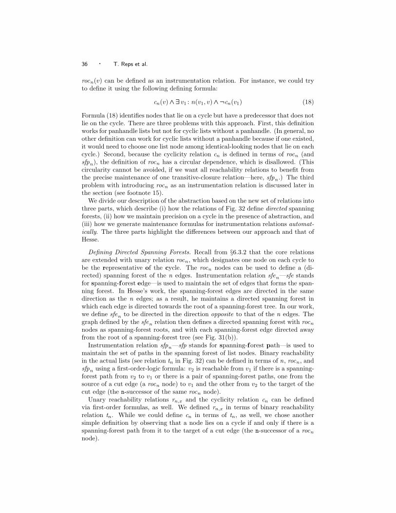
36 · T. Reps et al.
rocn(v) can be defined as an instrumentation relation. For instance, we could tryto define it using the following defining formula:
cn(v)∧ ∃ v1 : n(v1, v)∧ ¬cn(v1) (18)
Formula (18) identifies nodes that lie on a cycle but have a predecessor that does notlie on the cycle. There are three problems with this approach. First, this definitionworks for panhandle lists but not for cyclic lists without a panhandle. (In general, noother definition can work for cyclic lists without a panhandle because if one existed,it would need to choose one list node among identical-looking nodes that lie on eachcycle.) Second, because the cyclicity relation cn is defined in terms of rocn (andsfpn), the definition of rocn has a circular dependence, which is disallowed. (Thiscircularity cannot be avoided, if we want all reachability relations to benefit fromthe precise maintenance of one transitive-closure relation—here, sfpn.) The thirdproblem with introducing rocn as an instrumentation relation is discussed later inthe section (see footnote 15).
We divide our description of the abstraction based on the new set of relations intothree parts, which describe (i) how the relations of Fig. 32 define directed spanningforests, (ii) how we maintain precision on a cycle in the presence of abstraction, and(iii) how we generate maintenance formulas for instrumentation relations automat-ically. The three parts highlight the differences between our approach and that ofHesse.
Defining Directed Spanning Forests. Recall from §6.3.2 that the core relationsare extended with unary relation rocn, which designates one node on each cycle tobe the representative of the cycle. The rocn nodes can be used to define a (di-rected) spanning forest of the n edges. Instrumentation relation sfen—sfe standsfor spanning-forest edge—is used to maintain the set of edges that forms the span-ning forest. In Hesse’s work, the spanning-forest edges are directed in the samedirection as the n edges; as a result, he maintains a directed spanning forest inwhich each edge is directed towards the root of a spanning-forest tree. In our work,we define sfen to be directed in the direction opposite to that of the n edges. Thegraph defined by the sfen relation then defines a directed spanning forest with rocn
nodes as spanning-forest roots, and with each spanning-forest edge directed awayfrom the root of a spanning-forest tree (see Fig. 31(b)).
Instrumentation relation sfpn—sfp stands for spanning-forest path—is used tomaintain the set of paths in the spanning forest of list nodes. Binary reachabilityin the actual lists (see relation tn in Fig. 32) can be defined in terms of n, rocn, andsfpn using a first-order-logic formula: v2 is reachable from v1 if there is a spanning-forest path from v2 to v1 or there is a pair of spanning-forest paths, one from thesource of a cut edge (a rocn node) to v1 and the other from v2 to the target of thecut edge (the n-successor of the same rocn node).
Unary reachability relations rn,x and the cyclicity relation cn can be definedvia first-order formulas, as well. We defined rn,x in terms of binary reachabilityrelation tn. While we could define cn in terms of tn, as well, we chose anothersimple definition by observing that a node lies on a cycle if and only if there is aspanning-forest path from it to the target of a cut edge (the n-successor of a rocn
node).

Finite Differencing of Logical Formulas · 37
Fig. 31(b) shows 2-valued structure S31, which represents the store of Fig. 27(a)using the extended set of core and instrumentation relations. The relations prx andpr is will be explained shortly.
Preserving Node Ordering on a Cycle in the Presence of Abstraction. The factthat our techniques need to be applicable in the presence of abstraction introducesa complication that is not present in the setting studied by Hesse. His concernwas with the expressibility of certain properties within the confines of a logic withcertain syntactic restrictions. Our concern is with the ability to maintain precisionin the framework of canonical abstraction.
nu3 u4u2u1 n
rn,xrn,x
n,sfen
rocnrn,x,cnrn,y
n,sfen
sfen
nsfen
sfen
nsfe
n
n
sfen
yx
isnrn,x,cn
rn,y
rn,x,cnrn,y
u6
u5
rn,xrn,y
cn
Fig. 33. A 3-valued structure S#33 that is the
canonical abstraction of structure S#30 if relations
prx and pr is are not added to A and node u7 of
S#30 (represented by u5 in S#
33) is the rocn node.
Unary reachability relationsrn,x (one for every programvariable x) play a crucial rolein the analysis of programsthat manipulate acyclic linkedlists. In addition to keepingdisjoint lists summarized sep-arately, they keep list nodesthat have been visited during atraversal summarized separatelyfrom nodes that have not beenvisited: if x is the pointer usedto traverse the list, then thenodes that have been visited willhave value 0 for relation rn,x,while the nodes that have notbeen visited will have value 1. Ifa list contains a cycle, then all nodes on the cycle are reachable from the same setof variables, namely, all variables that point to any node in that list. As a result,the instrumentation relations discussed thus far cannot prevent nodes u4, u6, andu8 of S#
30 shown in Fig. 30 from being summarized together. Thus, assuming that
u7 is the rocn node, the canonical abstraction of S#30 is the 3-valued structure S#
33
shown in Fig. 33. The nodes represented by u4, u6, and u8 of S#30 are represented
by the single summary individual u6 in S#33. The symmetry hides all information
about the order of traversal via pointer variable y. Moreover, the values of the sfpn
relation (not shown in Fig. 33) lose precision because ancestors of the shared nodein the spanning tree are summarized together with its descendants in the spanningtree.
We break the symmetry of the nodes on a cycle using a general mechanism viaunary properties akin to unary reachability relations rn,x. In the definitions of rela-tions prx of Fig. 32, full reachability (relation tn) has been replaced with spanning-forest reachability (relation sfpn). The relations prx distinguish nodes according towhether or not they are reachable from program variable x along spanning-forestedges. The relation pr is is defined similarly but using instrumentation relation isn;pr is partitions the nodes of a panhandle list into ancestors and descendants of the
shared node in the spanning tree. Fig. 34 shows structure S#34, which is the canon-
ical abstraction of S#30 of Fig. 30, assuming that u7 is the rocn node. In S#
34, each

38 · T. Reps et al.
n n nnn n
x yn n
u3 u5u1 u4u2
n
prypris
prypris
pry
prxprypris
pry rocn
n
pryprisn n
u7u6
u8
Fig. 34. A 3-valued structure S#34 that is the canonical abstraction of structure S#
30 if node u7 is
the rocn node. S#34 represents panhandle lists of type XY , such as the store of Fig. 27(b). The
only instrumentation relations shown in the figure are prx, pry, and pr is . As in structure S#30
shown in Fig. 30, rn,x holds for all nodes, rn,y and cn hold for all nodes on the cycle, and isn
holds for u3.
of the nodes u4, u6, and u8 has a distinct vector of values for the relations pry andpr is , thus breaking the symmetry.14
Automatic Generation of Maintenance Formulas for Instrumentation Relations.In his thesis, Hesse gives hand-specified relation-maintenance formulas for a col-lection of relations that are used for maintaining a spanning-forest representationof possibly-cyclic linked lists. Instead of specifying relation-maintenance formulasby hand, we rely on finite differencing, as described in previous sections of thispaper, to generate maintenance formulas for all instrumentation relations. Finite-differencing-generated maintenance formulas have been effective in maintaining allrelations defined via first-order-logic formulas, i.e., all relations of Fig. 32 exceptsfpn. Additionally, under certain conditions, finite-differencing-generated mainte-nance formulas have been effective in maintaining relations defined via the reflexivetransitive closure of binary relations. Two conditions are necessary for this tech-nique to be applicable for maintaining relation sfpn:
Graph-shape condition. The graph defined by sfen must be acyclic or tree-shaped.
Unit-size-change condition. Each program statement must only change the graphof n edges by adding a single edge or deleting a single edge (but not both).
The graph-shape condition applies in our setting because the graph defined by sfen
defines a spanning forest (which is both acyclic and tree-shaped). The unit-size-change condition requires some discussion.
The relation sfen is defined in terms of n and rocn. While we have not yetdiscussed the relation-update formulas for core relation rocn, it should be clearthat the value of the relation rocn should only change in response to a change inthe value of a node’s n field. There are two types of statements that change the valueof the n field and thus may have an effect on the value of the sfen relation—namely,statements of the forms x->n = NULL and x->n = y. The former destroys the n
14Note that in the presence of multiple panhandles, we may be required to introduce finer distinc-tions to account for the possibility of multiple shared nodes on a cycle. These distinctions couldtake the form of a family of is-shared relations—one for each variable—to capture the panhandlethat contributes to sharing. We do not discuss a detailed solution to this problem here, as it willnot provide significant further insight.
Finite Differencing of Logical Formulas · 39
edge leaving the node pointed to by x, and the latter creates a new n-connectionfrom the node pointed to by x to the node pointed to by y. While both of thesestatements add or remove a single edge of the n relation, it is not necessarily thecase that they add or remove a single edge of the sfen relation. When interpreted
on logical structure S#34 of Fig. 34, statement y->n = NULL has the effect of deleting
the n edge leaving u5, an action that should result in the deletion of the sfen edgeentering u5 (not shown in the figure). However, to preserve the spanning-forestrepresentation, we need to ensure that rocn holds only for nodes that lie on a cycle,and that sfen represents spanning-forest edges. This requires setting the value ofrocn for u7 to 0 and adding an sfen edge from u8 to u7. Because, as this exampleillustrates, a language statement may result in the deletion of one sfen edge and theaddition of another, neither of the techniques from §6.1 and §6.2 for maintaininginstrumentation relations defined via RTC applies.
To work around this problem, the transformers associated with the statementsx->n = NULL and x->n = y each have two phases. In one phase, we apply the partof the transformer that corresponds to the relation n, and update the values of allinstrumentation relations. In the other phase, we apply the part of the transformerthat corresponds to the relation rocn, and update the values of all instrumentationrelations. As we explain below, each phase of the two transformers satisfies therequirement that the change adds a single edge or removes a single edge of the sfen
relation.15 Additionally, by paying attention to the order of phases, we ensure thatthe graph defined by the relation sfen remains acyclic and tree-shaped throughoutthe application of the transformers.
To preserve the graph-shape condition in the case of statement x->n = NULL, weapply the part of the transformer that corresponds to the relation n first:
τn,x−>n = NULL(v1, v2) = n(v1, v2)∧ ¬x(v1). (19)
Unless x points to a rocn node (or x->n is NULL), this phase results in the deletionof the sfen edge that enters the node pointed to by x. In the second phase, weapply the part of the transformer that corresponds to the relation rocn:
τrocn,x−>n = NULL(v) = rocn(v)∧ ∃ v1 : n(v, v1)∧ sfpn(v, v1). (20)
This phase sets the rocn property of the source ns of a cut edge to 0, if there is nolonger a spanning-forest path from ns to the target nt of the same cut edge. Whenthis happens and x does not point to ns, i.e., the cut edge is not being deleted, thisphase results in the addition of an sfen edge from nt to ns.
To preserve the graph-shape condition in the case of statement x->n = y, weapply the part of the transformer that corresponds to the relation rocn first:
τrocn,x−>n = y(v) = rocn(v)∨(x(v)∧ ∃ v1 : y(v1)∧ sfpn(v, v1)). (21)
If there is a spanning-forest path from node nx, pointed to by x, to node ny, pointedto by y, the statement creates a new cycle in the data structure. The update of
15The third problem with defining rocn as an instrumentation relation (alluded to earlier in thesection) is that we would lose the ability to apply the two parts of a transformer separately: thechange in the values of n would immediately trigger a change in the values of rocn. The resultingtransformer would not be able to satisfy the unit-size-change condition.
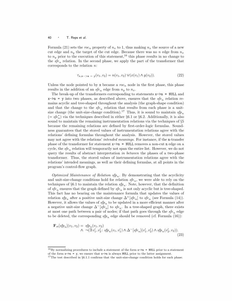
40 · T. Reps et al.
Formula (21) sets the rocn property of nx to 1, thus making nx the source of a newcut edge and ny the target of the cut edge. Because there was no n edge from nx
to ny prior to the execution of this statement,16 this phase results in no change tothe sfen relation. In the second phase, we apply the part of the transformer thatcorresponds to the relation n:
τn,x−>n = y(v1, v2) = n(v1, v2)∨(x(v1)∧ y(v2)). (22)
Unless the node pointed to by x became a rocn node in the first phase, this phaseresults in the addition of an sfen edge from ny to nx.
The break-up of the transformers corresponding to statements x->n = NULL andx->n = y into two phases, as described above, ensures that the sfen relation re-mains acyclic and tree-shaped throughout the analysis (the graph-shape condition)and that the change to the sfen relation that results from each phase is a unit-size change (the unit-size-change condition).17 Thus, it is sound to maintain sfpn
(= sfe∗n) via the techniques described in either §6.1 or §6.2. Additionally, it is also
sound to maintain the remaining instrumentation relations via the techniques of §5because the remaining relations are defined by first-order-logic formulas. Sound-ness guarantees that the stored values of instrumentation relations agree with therelations’ defining formulas throughout the analysis. However, the stored valuesmay not agree with the relations’ intended meanings. For instance, if the n-transferphase of the transformer for statement x->n = NULL removes a non-cut n edge on acycle, the sfen relation will temporarily not span the entire list. However, we do notquery the results of abstract interpretation in between the phases of a two-phasetransformer. Thus, the stored values of instrumentation relations agree with therelations’ intended meanings, as well as their defining formulas, at all points in theprogram’s control-flow graph.
Optimized Maintenance of Relation sfpn. By demonstrating that the acyclicityand unit-size-change conditions hold for relation sfen, we were able to rely on thetechniques of §6.1 to maintain the relation sfpn. Note, however, that the definitionof sfen ensures that the graph defined by sfen is not only acyclic but is tree-shaped.This fact has no bearing on the maintenance formula that updates the values ofrelation sfpn after a positive unit-size change ∆+[sfen] to sfen (see Formula (14)).However, it allows the values of sfpn to be updated in a more efficient manner aftera negative unit-size change ∆−[sfen] to sfen. In a tree-shaped graph, there existsat most one path between a pair of nodes; if that path goes through the sfen edgeto be deleted, the corresponding sfpn edge should be removed (cf. Formula (16)):
Fst[sfpn](v1, v2) = sfpn(v1, v2)∧ ¬(∃ v′1, v
′2 : sfpn(v1, v
′1)∧∆−[sfen](v′1, v
′2)∧ sfpn(v′2, v2)).
(23)
16By normalizing procedures to include a statement of the form x->n = NULL prior to a statementof the form x->n = y, we ensure that x->n is always NULL prior to the latter assignment.17The test described in §6.1.1 confirms that the unit-size-change condition holds for each phase.

Finite Differencing of Logical Formulas · 41
# of non-identity Performance
Category Test Program maintenance formulas Analysis Time (sec.) % increase
schemas # inst. Ref. FD FD
total TC non-TC acyc. tree acyc. tree
Search 2 0 2 2 0.30 0.30 0.31 1.10 1.90
GetLast 3 0 3 4 0.31 0.32 0.32 2.23 2.22
SLL DeleteAll 11 2 9 15 0.30 0.32 0.30 4.97 -0.13
Shape Reverse 12 2 10 16 0.43 0.49 0.44 12.69 1.99
Analysis Create 11 2 9 21 0.28 0.31 0.28 9.61 -0.60
Delete 12 2 10 39 1.13 2.13 1.23 87.90 7.76
Merge 11 2 9 64 1.77 3.67 1.96 107.27 10.42
Insert 12 2 10 72 1.19 2.03 1.31 70.43 9.67
DLL Append 15 2 13 50 1.76 1.78 1.77 1.13 0.57
Shape Delete 16 2 14 74 8.35 8.78 8.38 5.15 0.36
Analysis Splice 15 2 13 96 1.06 1.69 1.10 59.70 3.79
Binary InsertSorted 13 2 11 43 1.25 1.28 1.28 1.97 1.54
Tree Lindstrom 10 2 8 43 40.44 82.29 41.48 103.47 2.57
Shape DSW 10 2 8 52 101.30 180.20 109.51 77.89 8.15
Analysis DeleteSorted 13 2 11 554 75.26 409.31 97.71 443.85 29.69
ReverseSorted 18 2 16 23 0.47 0.54 0.49 13.05 2.58
BubbleSort 18 2 16 80 5.74 8.91 6.42 55.32 11.77
SLL BubbleSortBug 18 2 16 80 5.41 7.61 6.01 40.75 11.14
Sorting InsertSortBug2 18 2 16 87 5.19 17.57 6.09 238.55 17.04
InsertSort 18 2 16 88 5.65 18.55 6.66 228.26 17.95
InsertSortBug1 18 2 16 88 18.94 32.93 20.25 73.84 7.27
MergeSorted 18 2 16 91 2.26 4.22 2.53 86.35 11.46
Information Good Flow 12 2 10 66 13.59 23.28 15.37 71.30 13.59
Flow Bad Flow 12 2 10 86 78.05 180.85 94.92 131.70 21.79
Fig. 35. Results from using hand-crafted vs. automatically-generated maintenance formulas forinstrumentation relations.
7. EXPERIMENTAL EVALUATION
To evaluate the techniques presented in §5 and §6, we extended TVLA version2 to generate relation-maintenance formulas, and applied it to a test suite of fiveexisting analysis specifications, involving twenty-four programs, along with a varietyof different abstractions and properties to check (see Fig. 35). The experimentwas designed to determine what penalty is incurred when the relation-maintenanceformulas generated by our finite-differencing-based algorithm are used in place ofhand-crafted relation-maintenance formulas. In the experiment, we used the set ofhand-crafted relation-maintenance formulas that had been built up during severalyears of experience with TVLA. The idea was that if the penalty is low for theprograms, abstractions, and program properties in the test suite, that would beevidence that the penalty will be low for other examples—and that one can afford toforgo the effort of hand-crafting maintenance formulas for other analysis examples.
The test programs consisted of various operations on acyclic singly-linked lists,doubly-linked lists, binary trees, and binary-search trees, plus several sorting pro-grams [Lev-Ami et al. 2000]. The system was used to verify a variety of propertiesof the test programs. For instance, Reverse, an in-situ list-reversal program, mustpreserve list properties and lose no elements; InsertSorted and DeleteSorted mustpreserve binary-search-tree properties; InsertSort must return a sorted list; GoodFlow must not allow high-security input data to flow to a low-security output chan-nel. (Loginov et al. discuss the verification of stronger properties, such as the partialcorrectness of several of the algorithms [Loginov et al. 2005; Loginov 2006; Loginov

42 · T. Reps et al.
et al. 2007].)Lindstrom and DSW are two variants of Deutsch-Schorr-Waite, a constant-space
tree-traversal algorithm that uses destructive pointer rotation. For Lindstrom andDSW, we verified that the algorithms have no unsafe pointer operations or memoryleaks, and that the data structure produced at the end is, in fact, a binary tree.(Loginov et al. [2006] discuss the verification of the total correctness of Deutsch-Schorr-Waite—i.e., that the binary tree produced at the end is identical to the inputtree and that the algorithm terminates.)
A few of the programs contained bugs: for instance, InsertSortBug2 is an insert-sort program that ignores the first element of the list; BubbleBug is a bubble-sortprogram with an incorrect condition for swapping elements, which causes an infiniteloop if the input list contains duplicate data values. (See [Lev-Ami et al. 2000; Doret al. 2000; Lev-Ami and Sagiv 2000] for more details.)
In TVLA, the operational semantics of a programming language is defined byspecifying, for each kind of statement, an action schema to be used on outgoingCFG edges. Action schemas are instantiated according to a program’s statementinstances to create the CFG. For each combination of action schema and instru-mentation relation, a maintenance-formula schema must be provided. The numberof non-identity maintenance-formula schemas is reported in columns 3–5 of Fig. 35(grouped under the header “schemas”). In columns 4–5, they are broken down intothose whose defining formula contains an occurrence of RTC (under the header“TC”), and those that do not (under the header “non-TC”). Relation-maintenanceformulas produced by finite differencing are generally larger than the hand-craftedones. Because this affects analysis time, the number of instances of non-identitymaintenance-formula schemas is a meaningful size measure for our experiments.These numbers appear in column 6 (under the header “# inst.”). The number ofinstances of non-identity schemas for DeleteSorted is high because DeleteSortedincludes three inline expansions of the routine that finds the tree node that takesthe place of the deleted node.18
The data structures manipulated by all programs in our test suite are acyclic andtree-shaped, thus acyclic reachability maintenance (i.e., the technique described in§6.1), as well as tree-shaped reachability maintenance (i.e., the technique describedin §6.2), apply for the maintenance of reachability relations. In the absence of hand-crafted maintenance formulas for reachability relations in possibly-cyclic linked lists,we could not extend our experiments to cover the technique of §6.3. Instead, wevalidated that technique as part of the verification of properties of Reverse whenapplied to possibly-cyclic linked lists (see [Loginov et al. 2007]).
For each program in the test suite, we first ran the analysis using hand-craftedmaintenance formulas, to obtain a reference answer in which CFG nodes were an-notated with their final sets of logical structures. We then ran the analysis usingautomatically generated maintenance formulas with acyclic reachability mainte-nance (§6.1) and compared the result against the reference answer. For all 24 testprograms, the analysis using automatically generated formulas yielded answers iden-tical to the reference answers, thus establishing the same properties. Finally, we ran
18Work on interprocedural shape analysis provides a solution that does not require inline-expandedprograms [Rinetzky and Sagiv 2001; Rinetzky et al. 2005; Jeannet et al. 2004; 2010].

Finite Differencing of Logical Formulas · 43
the analysis using automatically generated maintenance formulas with tree-shapedreachability maintenance (§6.2) and compared the result against the reference an-swer. Again, for all 24 test programs, the analysis using automatically generatedformulas yielded answers identical to the reference answers, thus establishing thesame properties.
Columns 7–11 show performance data, which were collected on a 3GHz PC with3.7GB of RAM running CentOS 4 Linux. The column labeled “Ref.” gives the ref-erence times (i.e., when the hand-crafted maintenance formulas are used). Columnslabeled “acyc.” give the data for the analyses that used automatically generatedmaintenance formulas with acyclic reachability maintenance. Columns labeled“tree”give the data for the analyses that used automatically generated maintenanceformulas with tree-shaped reachability maintenance. (As stated above, for each testprogram the use of hand-crafted maintenance formulas, acyclic-reachability mainte-nance formulas, and tree-shaped reachability maintenance formulas all establishedidentical properties.) In each case, five runs were made; the longest and shortesttimes were discarded from each set, and the remaining three averaged. The geo-metric mean of the slowdowns when using the automatically generated formulaswith acyclic reachability maintenance was approximately 60%, with a median of55%, mainly due to the fact that the automatically generated formulas are largerthan the hand-crafted ones. The maximum slowdown was 444%. The highest slow-downs occurred in analyses of programs that involved deletions of edges in a datastructure’s graph.
Because the edge-deletion maintenance formulas produced by the tree-shapedreachability-maintenance technique are much smaller than those that are producedby acyclic reachability maintenance, our expectation was that the use of tree-shapedreachability-maintenance formulas would cause a much smaller slowdown. Thisexpectation was confirmed: the geometric mean of the slowdowns when using theautomatically generated formulas with tree-shaped reachability maintenance wasapproximately 8%, with a median of 7%. The maximum slowdown was 30%.19 Afew analyses were actually faster with the automatically generated formulas; thesespeedups are either due to random variation or are accidental benefits of subformulaorderings that are advantageous for short-circuit evaluation.
These results are encouraging. At least for abstractions of several common datastructures, they suggest that the algorithm for generating relation-maintenanceformulas from §5 and §6 is capable of automatically generating formulas that (i)are as precise as the hand-crafted ones, and (ii) have a tolerable effect on runtimeperformance.
The extended version of TVLA also uncovered several bugs in the hand-craftedformulas. A maintenance formula of the form µp,st(v1, . . . , vk) = p(v1, . . . , vk)is called an identity relation-maintenance formula. For each identity relation-maintenance formula in the hand-crafted specification, we checked that (after sim-plification) the corresponding generated relation-maintenance formula was also anidentity formula. Each inconsistency turned out to be an error in the hand-craftedspecification. We also found one instance of an incorrect non-identity hand-crafted
19We expect that some simple optimizations, such as caching the results from evaluating subfor-mulas, could reduce the slowdown further.

44 · T. Reps et al.
maintenance formula. (The measurements reported in Fig. 35 are based on cor-rected hand-crafted specifications.)
8. RELATED WORK
Our work addresses an instance of the following fundamental challenge in applyingabstract interpretation:
Given the concrete semantics for a language and a desired abstraction,how does one create sound abstract transformers?
In our context, a desired abstraction is specified by defining the set of instrumen-tation relations to use. The question is how to obtain sound relation-maintenanceformulas for use in the abstract transformer. A weakness of the original formu-lation of TVLA [Sagiv et al. 2002; Lev-Ami and Sagiv 2000] was that the userneeded to define relation-maintenance formulas by hand to specify how each struc-ture transformer affects each instrumentation relation. Past criticisms of TVLAbased on this deficiency [Ball et al. 2001; Møller and Schwartzbach 2001] are nolonger valid, at least for analyses that can be specified using formulas that defineacyclic relations (and also for some classes of formulas that define cyclic relations).With the algorithm presented in §5 and §6, the user’s responsibility is merely towrite the ψp formulas that define the set of instrumentation relations; appropriaterelation-maintenance formulas are then created automatically.
For certain situations [Graf and Saıdi 1997; Reps et al. 2004; Yorsh et al. 2004], itis known how to create best abstract transformers in the sense of [Cousot and Cousot1979]; that is, the abstract transformers created are the most precise transformersthat are possible, given the abstraction that is in use. Graf and Saıdi [1997] showedthat theorem provers can be used to generate best abstract transformers for abstractdomains that are fixed, finite, Cartesian products of Boolean values. (The use ofsuch domains is known as predicate abstraction; predicate abstraction is also used inSLAM [Ball et al. 2001] and other systems [Das et al. 1999].) Reps et al. [2004] gavea method—which applies to a broader class of abstract domains than predicate-abstraction domains—for computing the effect of applying the best transformer.Yorsh et al. [2004] gave a related method for abstract domains based on canonicalabstraction (i.e., for shape analysis). Both of those methods provide a way to applya best transformer, but do not produce an explicit representation of the abstracttransformer. Moreover, they each involve a sequence of calls on an appropriatedecision procedure (or semi-decision procedure). In the case of shape analysis, themethod of Yorsh et al. [2004] is generally much more expensive than the algorithmdescribed in §5 and §6.
In contrast, the abstract transformers created using the algorithm described in§5 and §6 are not best transformers; however, the algorithm uses only very simple,linear-time, recursive tree-traversal procedures, whereas the theorem provers used inpredicate abstraction are not even guaranteed to terminate. Moreover, our settingmakes available much richer abstract domains than the ones offered by predicateabstraction, and experience to date has been that very little precision is lost (usingonly good abstract transformers) once the right instrumentation relations have beenidentified.

Finite Differencing of Logical Formulas · 45
Other work on automatically creating abstract transformers includes the follow-ing:
—Methods based on semantic reinterpretation [Mycroft and Jones 1985; 1986; Niel-son 1989; Malmkjær 1993; Lim and Reps 2008] factor the concrete semantics ofa language into two parts: (i) a client specification, and (ii) a semantic core. Theinterface to the core consists of certain base types, function types, and opera-tors, and the client is expressed in terms of this interface. Such an organizationpermits the core to be reinterpreted to produce an alternative semantics for thesubject language.
Semantic reinterpretation is convenient in that soundness of the entire abstractsemantics can be established via purely local soundness arguments for each of thereinterpreted operators. However, semantic reinterpretation has a purely local—and hence myopic—view of the behavior of a transformer, and hence can lead toabstract transformers that lose a substantial amount of precision. In contrast, thealgorithm presented in §5 and §6 is generally able to retain an appropriate amountof precision because the finite-differencing approach to obtaining an abstracttransformer for a concrete transformer τ aims to reuse as much information aspossible from the pre-state structure, and thereby avoids formula-reevaluationoperations for tuples of a relation whose values cannot be changed by τ .
—Scherpelz et al. [2007] developed a method for creating abstract transformersfor use with parameterized predicate abstraction [Cousot 2003]. It uses weakestliberal precondition (WLP) followed by heuristics that approximate how combi-nations of pre-state relations imply the WLP of a post-state relation with respectto a transformer τ . Generating the abstract transformer for a (nullary) instru-mentation relation p in vocabulary R involves two steps (where p is defined bythe nullary formula ψp()):
(1) Create the formula ϕ = WLP(τ, ψp()).(2) Find a Boolean combination µp,τ [R] of the pre-state relations such that if
µp,τ [R] holds in the pre-state then ϕ must also hold in the pre-state (andhence p must hold in the post-state).
The abstract transformer is a function that sets the value of p in the post-stateaccording to whether µp,τ [R] holds in the pre-state.Because WLP performs substitution on ψp(), the formula created by step (1)
is related to the naıve relation-maintenance formula defined in Eqn. (5) of §3.Step (2) applies several heuristics to ϕ to produce one or more strengtheningsof ϕ; step (2) returns the disjunction of the strengthened variants of ϕ. Incontrast, the algorithm presented in §5 and §6 does not operate by trying tostrengthen the naıve relation-maintenance formula; instead, it uses a systematicapproach—based on finite differencing of p’s defining formula ψp()—to identifyhow τ changes p’s value. Moreover, our method is not restricted to nullaryinstrumentation relations: it applies to relations of arbitrary arity.A special case of canonical abstraction occurs when no abstraction relations are
used at all, in which case all individuals of a logical structure are collapsed toa single individual. When this is done, in almost all structures the only usefulinformation remaining resides in the nullary core and instrumentation relations.Predicate abstraction can be seen as going one step further, retaining only the

46 · T. Reps et al.
nullary instrumentation relations (and no abstracted core relations). However,to be able to evaluate a “Future” formula—as defined in Eqns. (11) and (12)
of §5—such as Fτ [p]def
= p ? ¬∆−τ [p] : ∆+
τ [p], one generally needs the pre-stateabstract structure to hold (abstracted) core relations. From this standpoint, ourmethod and that of Scherpelz et al. [2007] are incomparable; they have differentgoals, and neither can be said to subsume the other.
Paige and Koenig [1982] studied how finite-differencing transformations of ap-plicative set-former expressions could be exploited to optimize loops in very-high-level languages, such as SETL. Liu et al. used related program-transformationmethods in the setting of a functional programming language to derive incrementalalgorithms for various problems from the specifications of exhaustive algorithms[Liu and Teitelbaum 1995; Liu et al. 1996]. In their work, the goal is to maintainthe value of a function F (x) as the input x undergoes small changes. The methodsdescribed in §5 and §6 address a similar kind of incremental-computation problem,except that the language in which the exhaustive and incremental versions of theproblem are expressed is first-order logic with reflexive transitive closure.
The finite-differencing operators defined in §5 and §6 are most closely related to anumber of previous papers on logic and databases: finite-difference operators for thepropositional case were studied by Akers [1959] and Sharir [1982]. Previous workon incrementally maintaining materialized views in databases [Gupta and Mumick1999], “first-order incremental evaluation schemes (FOIES)” [Dong and Su 1995],and “dynamic descriptive complexity” [Patnaik and Immerman 1997] has also ad-dressed the problem of maintaining one or more auxiliary relations after new tuplesare inserted into or deleted from the base relations. In databases, view mainte-nance is solely an optimization; the correct information can always be obtained byreevaluating the formula. In the abstract-interpretation context, where abstractionhas been performed, this is no longer true: reevaluating a formula in the local (3-valued) state can lead to a drastic loss of precision. Thus, one aspect that setsour work apart from previous work is the goal of developing a finite-differencingtransformation suitable for use when abstraction has been performed.
In §6.3.2, we compared our work to that of Hesse [2003], which is closest in spiritto our techniques for maintaining reachability information in possibly-cyclic linkedlists. Below, we discuss a few approaches that bear resemblance to ours in thatthey attempt to translate or simulate a data structure that cannot be handled bysome core techniques into one that can.
The idea of using spanning-tree representations for specifying or reasoning aboutdata structures that are “close to trees” is not new. Klarlund and Schwartzbachintroduced graph types, which can be used to specify some common non-tree-shaped data structures in terms of a spanning-tree backbone and regular expressionsthat specify where non-backbone edges occur within the backbone [Klarlund andSchwartzbach 1993]. Examples of data structures that can be specified by graphtypes are doubly-linked lists and threaded trees. A panhandle list cannot be spec-ified by a graph type because in a graph type the location of each non-backboneedge has to be defined in terms of the backbone using a regular expression, and aregular expression cannot be used to specify the existence of a backedge to somenode that occurs earlier in the list. In the PALE project [Møller and Schwartzbach

Finite Differencing of Logical Formulas · 47
2001], which incorporates work on graph types, automated reasoning about pro-grams that manipulate data structures specified as graph types can be carried outusing a decision procedure for monadic second-order logic. Unfortunately, the deci-sion procedure has non-elementary complexity. An advantage of our approach overthat of PALE is that we do not rely on the use of a decision procedure.
Immerman et al. [2004] presented structure simulation, a technique that broadensthe applicability of decision procedures to a larger class of data structures. Undercertain conditions, it allows data structures that cannot be reasoned about usingdecidable logics to be translated into data structures that can, with the translationexpressed as a first-order-logic formula. Unlike graph types, structure simulation iscapable of specifying panhandle lists. However, this technique shares a limitation ofgraph types because it relies on decision procedures for automated reasoning aboutprograms.
Manevich et al. [2005] specified abstractions (in canonical-abstraction andpredicate-abstraction forms) for showing safety properties of programs that manip-ulate possibly-cyclic linked lists. By maintaining reachability within list segmentsthat are not interrupted by nodes that are shared or pointed to by a variable, theyare able to break the symmetry of a cycle. The definition of several key instrumen-tation relations in that work makes use of transitive-closure formulas that cannotbe handled precisely by finite differencing. As a result, a drawback of that work isthe need to define some relation-maintenance formulas by hand. Another drawbackis the difficulty of reasoning about reachability (in a list) from a program vari-able (see reachability relations rn,x of Fig. 32). Because in [Manevich et al. 2005]reachability in a list has to be expressed in terms of reachability over a sequence ofuninterrupted segments, a formula that expresses the reachability of node v fromprogram variable x in a list has to enumerate all permutations of other programvariables that may act as interruptions on a path from x to v in the list.
A number of past approaches to the analysis of programs that manipulate linkedlists relied on first-order axiomatizations of reachability information. All of theseapproaches involved the use of first-order-logic decision procedures. While our ap-proach does not have this limitation, it is instructive to compare our work withthose approaches that included mechanisms for breaking the symmetry on a cycle.Nelson [1983] defined a set of first-order axioms that describe the ternary reacha-bility relation rn(u, v, w), which has the meaning: w is reachable from u along nedges without encountering v. The use of this relation alone is not sufficient in oursetting because in the presence of abstraction we require unary distinctions (suchas the relations prx and pr is of Fig. 32) to break the symmetry. Additionally, themaintenance of ternary relations is more expensive than the maintenance of binaryrelations. Lahiri and Qadeer [2006] specify a collection of first-order axioms thatare sufficient to verify properties of procedures that perform a single change to acyclic list, e.g., the removal of an element. They also verify properties of in-situlist reversal, albeit under the assumption that the input list is acyclic. In a recentpublication, we describe a case study in which we use the techniques developed in§6.3 to verify the total correctness (partial correctness and termination) of Reversewhen applied to any linked list, including cyclic and panhandle lists [Loginov et al.2007]. Lahiri and Qadeer break the symmetry of cycles in a similar fashion to how itis done by Manevich et al. [2005]: the blocking cells of Lahiri and Qadeer [2006] are
48 · T. Reps et al.
a subset of the interruptions of Manevich et al. [2005]. The blocking cells includeonly the set of head variables—program variables that act as heads of lists used inthe program. This set has to be maintained carefully by the user to (i) satisfy thesystem’s definition of acceptable (well-founded) lists, (ii) allow the system to ver-ify useful postconditions, and (iii) avoid falling prey to the difficulty—which arisesin the work of Manevich et al. [2005]—of expressing reachability in the list. Thecurrent mechanism of Lahiri and Qadeer [2006] is insufficient for reasoning aboutpanhandle lists because the set of blocking cells does not include shared nodes.This limitation can be partially addressed by generalizing the set of blocking cellsto mimic interruptions of Manevich et al. [2005] more faithfully. However, this maymake it more difficult to satisfy points (ii) and (iii) above. As in our work, Lahiriand Qadeer rely on the insight that reachability information can be maintained infirst-order logic. They use a collection of manually-specified update formulas thatdefine how their relations are affected by the statements of the language and the(user-inserted) statements that manage the set of head variables.
Distefano et al. [2006] presented a shape-analysis algorithm for singly-linked listsbased on separation logic. As shown by Reynolds [2002], one of the advantagesof separation logic is that, for some programs, it can be used to specify invariantsin an intuitive way. In most simple list-manipulating programs, the invariants aremuch more succinct than ones produced by TVLA [Yorsh et al. 2007].20 Also, asshown by Ishtiaq and O’Hearn [2001], the separating conjunction of separation logicpresents a simpler way to express postconditions than is possible in the frameworkof Sagiv et al. [2002] (see also [Jeannet et al. 2010]).
However, the framework of Sagiv et al. provides several benefits compared withexisting domains based on separation logic (“separation domains”):
—The framework of Sagiv et al. handles arbitrary imperative programs, and canprove arbitrary properties that can be expressed in first-order logic with reflexivetransitive closure (including numeric properties [Gopan et al. 2004; Gopan et al.2005]). In contrast, existing separation domains concentrate on proving memorysafety and preservation of data-structure invariants in linked lists.
—The framework of Sagiv et al. can be applied to arbitrary data structures, whereasexisting separation domains can be applied to data structures without sharing(e.g., acyclic singly-linked lists and binary trees) and data structures with sharingthat can be defined explicitly (e.g., binary trees with parent pointers), but notto data structures that exhibit more complex sharing patterns (e.g., DAGs).
—Canonical abstraction is based on an intuitive abstraction principle. Moreover,results can be rendered in a natural way (see §2.2). Both features make it easierto understand where information is lost, compared with results obtained fromtools that use separation domains.
—For programs that manipulate data structures beyond singly-linked lists, and forproving properties beyond memory safety, it is challenging to guarantee that ananalysis using a separation domain terminates: the abstract domain is infinite,
20Yorsh et al. [2007] presented a method that, given a 3-valued structure S#, creates a formulaϕ[S#] that is satisfied by exactly the set of structures that S# represents. For most 3-valuedstructures, such formulas are quite complicated.

Finite Differencing of Logical Formulas · 49
and a widening operation is not known that guarantees that the analysis willterminate in a finite number of iterations. This situation is the case in all existingseparation domains, e.g., the one described by Berdine et al. [2007]. In contrast,abstract domains based on canonical abstraction are finite, and hence terminationis guaranteed.
The techniques used to create abstract transformers for canonical-abstraction do-mains and separation domains are quite different. In our approach, the next stateis determined using three primitives (see §2.2.2 and [Sagiv et al. 2002]): (i) partialconcretization (or partial model enumeration) via the focus operation, (ii) formulaevaluation, using the finite-differencing-based formulas created by the techniquespresented in §5 and §6, and (iii) very lightweight logical reasoning via the coerceoperation. Analyses based on separation logic use specialized decision proceduresand formula-normalization procedures. Existing tools based on separation domainsspend a lot of time in formula normalization and in entailment checks.21 In part,this is because the separating conjunction does not distribute over ordinary logicalconjunction, but the primary reason for the high cost is that the separating con-junction involves an implicit second-order quantification. Consequently, the overallcost of an analysis specified using the framework of Sagiv et al. can be comparableto—or even lower—than that of an analysis based on a separation domain. (For acomparison, see [Bogudlov et al. 2007b].)
9. CONCLUSIONS
This paper addresses a fundamental challenge that arises in abstract interpretation:
Given the concrete semantics for a language and a desired abstraction,how does one create the associated abstract transformers?
This challenge arises in program-analysis problems in which the semantics of state-ments is expressed using logical formulas that describe changes to core-relationvalues. When instrumentation relations have been introduced to refine an abstrac-tion, the challenge is to reflect the changes in core-relation values in the values of theinstrumentation relations. The algorithm presented in this paper provides a wayto create formulas that maintain correct values for the instrumentation relations,and thereby provides a way to generate—completely automatically—the part of thetransformers of an abstract semantics that deals with instrumentation relations.
The work described in this paper opened the way for TVLA to be extended tosupport automatic abstraction refinement [Loginov et al. 2005; Loginov 2006]. Theidea is to start the analyzer with a crude abstraction, and use the results of analysisruns that fail to establish a definite answer (about whether the property of interestdoes or does not hold) as feedback about how the abstraction should be refined.
21In the instantiation of the framework of Sagiv et al. that we extended in this work—namely,TVLA version 2—the coerce operation dominates the cost of analysis. In our experiments, exe-cution of coerce accounted for 56%-98% of analysis time, with a mean of 72%. Aggregated overall test cases, execution of coerce accounted for 85% of the total analysis time. Bogudlov et al.studied the cost of key operations in TVLA. They achieved substantial speedups (as much as50-fold) due to a number of optimizations of the coerce operation. The reader is referred to theirtool paper and the accompanying technical report for more details [Bogudlov et al. 2007b; 2007a].

50 · T. Reps et al.
Abstraction refinement had previously been used in the model-checking commu-nity [Kurshan 1994; Clarke et al. 2000; Ball and Rajamani 2001]; however, findingan analog of this that was suitable for TVLA was a challenging problem becausecanonical abstraction is considerably more sophisticated than the abstractions usedby the model-checking community: in particular, predicate abstraction [Graf andSaıdi 1997] can be viewed as the degenerate case of canonical abstraction in whichonly nullary relations are retained [Reps et al. 2004, §4]. Because of this difference,we found that we had to use mechanisms that were completely different from thoseused in tools such as SLAM [Ball and Rajamani 2001], BLAST [Henzinger et al.2002], and Magic [Chaki et al. 2003]. Our solution involved using inductive logicprogramming to discover an appropriate set of instrumentation relations that refinethe abstraction in use [Loginov et al. 2005; Loginov 2006]. Finite-differencing is acrucial enabling technique in this approach because it provides the ability to createrelation-maintenance formulas automatically after refinement has been performed.
Finally, although the work described in the paper was motivated by a problemthat arose in work on static analysis based on 3-valued logic, any method in whichsystems are described as evolving (2-valued or 3-valued) logical structures—e.g.,Alloy [Jackson 2006] or Abstract State Machines [Boerger and Staerk 2003]—maybe able to benefit from these techniques.
Acknowledgments. We are grateful to W. Hesse, N. Immerman, T. Lev-Ami, andR. Wilhelm for their comments and suggestions concerning this work. R. Manevichprovided invaluable help with TVLA.
REFERENCES
Akers, Jr., S. 1959. On a theory of Boolean functions. J. Soc. Indust. Appl. Math. 7, 4 (Decem-ber), 487–498.
Ball, T., Majumdar, R., Millstein, T., and Rajamani, S. 2001. Automatic predicate abstrac-tion of C programs. In Prog. Lang. Design and Impl. 203–213.
Ball, T. and Rajamani, S. 2001. Automatically validating temporal safety properties of inter-faces. In SPIN Workshop. 103–122.
Berdine, J., Calcagno, C., Cook, B., Distefano, D., O’Hearn, P., Wies, T., and Yang, H.2007. Shape analysis for composite data structures. In Computer Aided Verif. 178–192.
Boerger, E. and Staerk, R. 2003. Abstract State Machines: A Method for High-Level SystemDesign and Analysis. Springer.
Bogudlov, I., Lev-Ami, T., Reps, T., and Sagiv, M. 2007a. Revamping TVLA: Making para-metric shape analysis competitive. Tech. Rep. TR-2007-01-01, Tel-Aviv Univ., Tel-Aviv, Israel.
Bogudlov, I., Lev-Ami, T., Reps, T., and Sagiv, M. 2007b. Revamping TVLA: Making para-metric shape analysis competitive (tool paper). In Computer Aided Verif. 221–225.
Chaki, S., Clarke, E., Groce, A., Jha, S., and Veith, H. 2003. Modular verification of softwarecomponents in C. In Int. Conf. on Softw. Eng. 385–395.
Clarke, E., Grumberg, O., Jha, S., Lu, Y., and Veith, H. 2000. Counterexample-guidedabstraction refinement. In Computer Aided Verif. 154–169.
Cousot, P. 2003. Verification by abstract interpretation. In Verification: Theory and Practice.243–268.
Cousot, P. and Cousot, R. 1977. Abstract interpretation: A unified lattice model for staticanalysis of programs by construction of approximation of fixed points. In Princ. of Prog. Lang.238–252.
Cousot, P. and Cousot, R. 1979. Systematic design of program analysis frameworks. In Princ.of Prog. Lang. 269–282.

Finite Differencing of Logical Formulas · 51
Das, S., Dill, D., and Park, S. 1999. Experience with predicate abstraction. In Computer Aided
Verif. 160–171.
Distefano, D., O’Hearn, P., and Yang, H. 2006. A local shape analysis based on separationlogic. In Tools and Algs. for the Construct. and Anal. of Syst. 287–302.
Dong, G. and Su, J. 1995. Incremental and decremental evaluation of transitive closure by
first-order queries. Inf. and Comp. 120, 101–106.
Dong, G. and Su, J. 2000. Incremental maintenance of recursive views using relational calcu-lus/SQL. SIGMOD Record 29, 1 (Mar.), 44–51.
Dor, N., Rodeh, M., and Sagiv, M. 2000. Checking cleanness in linked lists. In Static AnalysisSymp. 115–134.
Goldstine, H. 1977. A History of Numerical Analysis. Springer-Verlag.
Gopan, D., DiMaio, F., Dor, N., Reps, T., and Sagiv, M. 2004. Numeric domains with sum-marized dimensions. In Tools and Algs. for the Construct. and Anal. of Syst. 512–529.
Gopan, D., Reps, T., and Sagiv, M. 2005. A framework for numeric analysis of array operations.In Princ. of Prog. Lang. 338–350.
Graf, S. and Saıdi, H. 1997. Construction of abstract state graphs with PVS. In ComputerAided Verif. 72–83.
Gupta, A. and Mumick, I., Eds. 1999. Materialized Views: Techniques, Implementations, andApplications. The M.I.T. Press, Cambridge, MA.
Henzinger, T., Jhala, R., Majumdar, R., and Sutre, G. 2002. Lazy abstraction. In Princ. ofProg. Lang. 58–70.
Hesse, W. 2003. Dynamic computational complexity. Ph.D. thesis, Dept. of Computer Science,University of Massachusetts, Amherst, MA.
Immerman, N., Rabinovich, A., Reps, T., Sagiv, M., and Yorsh, G. 2004. Verification viastructure simulation. In Computer Aided Verif. 281–294.
Ishtiaq, S. and O’Hearn, P. 2001. BI as an assertion language for mutable data structures. InPrinc. of Prog. Lang. 14–26.
Jackson, D. 2006. Software Abstractions: Logic, Language, and Analysis. The M.I.T. Press.
Jeannet, B., Loginov, A., Reps, T., and Sagiv, M. 2004. A relational approach to interproce-dural shape analysis. In Static Analysis Symp. 246–264.
Jeannet, B., Loginov, A., Reps, T., and Sagiv, M. 2010. A relational approach to interproce-dural shape analysis. Trans. on Prog. Lang. and Syst. 32, 2 (Jan.).
Klarlund, N. and Schwartzbach, M. 1993. Graph types. In Princ. of Prog. Lang. 196–205.
Kurshan, R. 1994. Computer-Aided Verification of Coordinating Processes. Princeton Univ.Press.
Lahiri, S. and Qadeer, S. 2006. Verifying properties of well-founded linked lists. In Princ. ofProg. Lang. 115–126.
Lev-Ami, T., Reps, T., Sagiv, M., and Wilhelm, R. 2000. Putting static analysis to work forverification: A case study. In Int. Symp. on Softw. Testing and Analysis. 26–38.
Lev-Ami, T. and Sagiv, M. 2000. TVLA: A system for implementing static analyses. In StaticAnalysis Symp. 280–301.
Lim, J. and Reps, T. 2008. A system for generating static analyzers for machine instructions. InComp. Construct. 36–52.
Liu, Y., Stoller, S., and Teitelbaum, T. 1996. Discovering auxiliary information for incrementalcomputation. In Princ. of Prog. Lang. 157–170.
Liu, Y. and Teitelbaum, T. 1995. Systematic derivation of incremental programs. Sci. of Comp.Program. 24, 2 (Feb.), 1–39.
Loginov, A. 2006. Refinement-based program verification via three-valued-logic analysis. Ph.D.thesis, Comp. Sci. Dept., Univ. of Wisconsin, Madison, WI. Tech. Rep. 1574.
Loginov, A., Reps, T., and Sagiv, M. 2005. Abstraction refinement via inductive learning. InComputer Aided Verif. 519–533.
Loginov, A., Reps, T., and Sagiv, M. 2006. Automated verification of the Deutsch-Schorr-Waitetree-traversal algorithm. In Static Analysis Symp. 261–279.

52 · T. Reps et al.
Loginov, A., Reps, T., and Sagiv, M. 2007. Refinement-based verification for possibly-cyclic
lists. In Program Analysis and Compilation, Theory and Practice: Essays Dedicated to ReinhardWilhelm. 247–272.
Malmkjær, K. 1993. Abstract interpretation of partial-evaluation algorithms. Ph.D. thesis, Dept.of Comp. and Inf. Sci., Kansas State Univ., Manhattan, KS.
Manevich, R., Yahav, E., Ramalingam, G., and Sagiv, M. 2005. Predicate abstraction andcanonical abstraction for singly-linked lists. In Verif., Model Checking, and Abs. Interp. 181–198.
McMillan, K. 1999. Verification of infinite state systems by compositional model checking. InCorrect Hardware Design and Verification Methods (CHARME). 219–234.
Michie, D. 1968. Memo functions and machine learning. Nature 218, 19–22.
Møller, A. and Schwartzbach, M. 2001. The pointer assertion logic engine. In Prog. Lang.Design and Impl. 221–231.
Mycroft, A. and Jones, N. 1985. A relational framework for abstract interpretation. In Programsas Data Objects. 156–171.
Mycroft, A. and Jones, N. 1986. Data flow analysis of applicative programs using minimalfunction graphs. In Princ. of Prog. Lang. 296–306.
Nelson, G. 1983. Verifying reachability invariants of linked structures. In Princ. of Prog. Lang.38–47.
Nielson, F. 1989. Two-level semantics and abstract interpretation. Theor. Comp. Sci. 69, 2(Dec.), 117–242.
Paige, R. and Koenig, S. 1982. Finite differencing of computable expressions. Trans. on Prog.Lang. and Syst. 4, 3 (July), 402–454.
Patnaik, S. and Immerman, N. 1997. Dyn-FO: A parallel, dynamic complexity class. J. Comput.Syst. Sci. 55, 2 (Oct.), 199–209.
Reps, T., Loginov, A., and Sagiv, M. 2002. Semantic minimization of 3-valued propositionalformulae. In Logic in Comp. Sci. 40–54.
Reps, T., Sagiv, M., and Loginov, A. 2003. Finite differencing of logical formulas for staticanalysis. In European Symp. On Programming. 380–398.
Reps, T., Sagiv, M., and Wilhelm, R. 2004. Static program analysis via 3-valued logic. InComputer Aided Verif. 15–30.
Reps, T., Sagiv, M., and Yorsh, G. 2004. Symbolic implementation of the best transformer. InVerif., Model Checking, and Abs. Interp. 252–266.
Reynolds, J. 2002. Separation Logic: A logic for shared mutable data structures. In Logic inComp. Sci. 55–74.
Rinetzky, N., Bauer, J., Reps, T., Sagiv, M., and Wilhelm, R. 2005. A semantics for procedurelocal heaps and its abstractions. In Princ. of Prog. Lang. 296–309.
Rinetzky, N. and Sagiv, M. 2001. Interprocedural shape analysis for recursive programs. InComp. Construct. 133–149.
Sagiv, M., Reps, T., and Wilhelm, R. 2002. Parametric shape analysis via 3-valued logic. Trans.on Prog. Lang. and Syst. 24, 3, 217–298.
Scherpelz, E., Lerner, S., and Chambers, C. 2007. Automatic inference of optimizer flowfunctions from semantics meanings. In Prog. Lang. Design and Impl. 135–145.
Sharir, M. 1982. Some observations concerning formal differentiation of set theoretic expressions.Trans. on Prog. Lang. and Syst. 4, 2 (April), 196–225.
TVLA. TVLA system. “www.cs.tau.ac.il/∼tvla/”.
van Fraassen, B. 1966. Singular terms, truth-value gaps, and free logic. J. Phil. 63, 17 (Sept.),481–495.
Yorsh, G., Reps, T., and Sagiv, M. 2004. Symbolically computing most-precise abstract oper-ations for shape analysis. In Tools and Algs. for the Construct. and Anal. of Syst. 530–545.
Yorsh, G., Reps, T., Sagiv, M., and Wilhelm, R. 2007. Logical characterizations of heapabstractions. Trans. on Comp. Logic 8, 1 (Jan.).
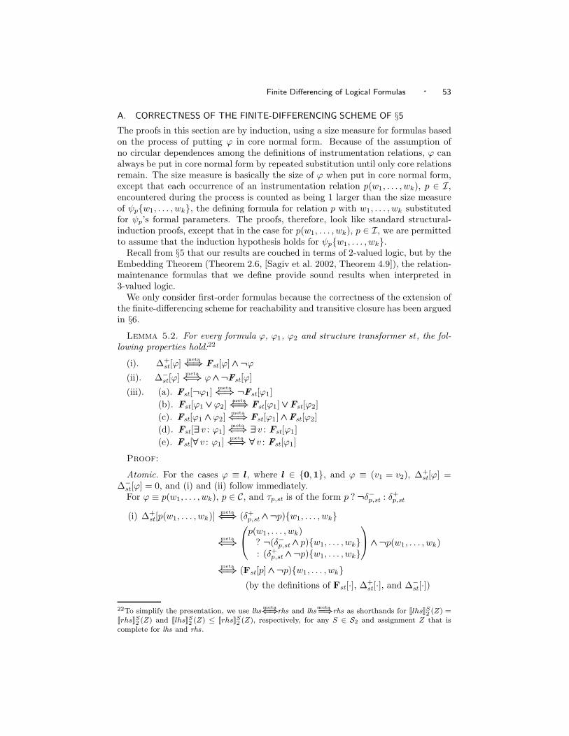
Finite Differencing of Logical Formulas · 53
A. CORRECTNESS OF THE FINITE-DIFFERENCING SCHEME OF §5
The proofs in this section are by induction, using a size measure for formulas basedon the process of putting ϕ in core normal form. Because of the assumption ofno circular dependences among the definitions of instrumentation relations, ϕ canalways be put in core normal form by repeated substitution until only core relationsremain. The size measure is basically the size of ϕ when put in core normal form,except that each occurrence of an instrumentation relation p(w1, . . . , wk), p ∈ I,encountered during the process is counted as being 1 larger than the size measureof ψp{w1, . . . , wk}, the defining formula for relation p with w1, . . . , wk substitutedfor ψp’s formal parameters. The proofs, therefore, look like standard structural-induction proofs, except that in the case for p(w1, . . . , wk), p ∈ I, we are permittedto assume that the induction hypothesis holds for ψp{w1, . . . , wk}.
Recall from §5 that our results are couched in terms of 2-valued logic, but by theEmbedding Theorem (Theorem 2.6, [Sagiv et al. 2002, Theorem 4.9]), the relation-maintenance formulas that we define provide sound results when interpreted in3-valued logic.
We only consider first-order formulas because the correctness of the extension ofthe finite-differencing scheme for reachability and transitive closure has been arguedin §6.
Lemma 5.2. For every formula ϕ, ϕ1, ϕ2 and structure transformer st, the fol-lowing properties hold:22
(i). ∆+st[ϕ]
meta
⇐⇒ Fst[ϕ] ∧ ¬ϕ
(ii). ∆−st[ϕ]
meta
⇐⇒ ϕ∧¬Fst[ϕ]
(iii). (a). Fst[¬ϕ1]meta
⇐⇒ ¬Fst[ϕ1]
(b). Fst[ϕ1 ∨ϕ2]meta
⇐⇒ Fst[ϕ1] ∨Fst[ϕ2]
(c). Fst[ϕ1 ∧ϕ2]meta
⇐⇒ Fst[ϕ1] ∧Fst[ϕ2]
(d). Fst[∃ v : ϕ1]meta
⇐⇒ ∃ v : Fst[ϕ1]
(e). Fst[∀ v : ϕ1]meta
⇐⇒ ∀ v : Fst[ϕ1]
Proof:
Atomic. For the cases ϕ ≡ l, where l ∈ {0,1}, and ϕ ≡ (v1 = v2), ∆+st[ϕ] =
∆−st[ϕ] = 0, and (i) and (ii) follow immediately.For ϕ ≡ p(w1, . . . , wk), p ∈ C, and τp,st is of the form p ? ¬δ−p,st : δ+p,st
(i) ∆+st[p(w1, . . . , wk)]
meta
⇐⇒ (δ+p,st ∧¬p){w1, . . . , wk}
meta
⇐⇒
p(w1, . . . , wk)? ¬(δ−p,st ∧ p){w1, . . . , wk}: (δ+p,st ∧¬p){w1, . . . , wk}
∧¬p(w1, . . . , wk)
meta
⇐⇒ (Fst[p] ∧¬p){w1, . . . , wk}
(by the definitions of Fst[·], ∆+st[·], and ∆−
st[·])
22To simplify the presentation, we use lhsmeta⇐⇒rhs and lhs
meta=⇒rhs as shorthands for [[lhs]]S2 (Z) =
[[rhs]]S2 (Z) and [[lhs]]S2 (Z) ≤ [[rhs]]S2 (Z), respectively, for any S ∈ S2 and assignment Z that iscomplete for lhs and rhs.

54 · T. Reps et al.
(ii) ∆−st[p(w1, . . . , wk)]
meta
⇐⇒ (δ−p,st ∧ p){w1, . . . , wk}
meta
⇐⇒ p{w1, . . . , wk}∧
p(w1, . . . , wk)? (δ−p,st ∧ p){w1, . . . , wk}: ¬(δ+p,st ∧ ¬p){w1, . . . , wk}
meta
⇐⇒ p{w1, . . . , wk}∧¬
p(w1, . . . , wk)? ¬(δ−p,st ∧ p){w1, . . . , wk}: (δ+p,st ∧ ¬p){w1, . . . , wk}
meta
⇐⇒ (p∧¬Fst[p]){w1, . . . , wk}
(by the definitions of Fst[·], ∆+st[·], and ∆−
st[·])
For ϕ ≡ p(w1, . . . , wk), p ∈ C, and τp,st is of the form p∨ δp,st or δp,st ∨ p
(i) ∆+st[p(w1, . . . , wk)]
meta
⇐⇒ (δp,st ∧¬p){w1, . . . , wk}
meta
⇐⇒(p(w1, . . . , wk) ? ¬0 : (δp,st ∧¬p){w1, . . . , wk})
∧ ¬p(w1, . . . , wk)meta
⇐⇒ (Fst[p] ∧¬p){w1, . . . , wk}
(by the definitions of Fst[·], ∆+st[·], and ∆−
st[·])
(ii) ∆−st[p(w1, . . . , wk)]
meta
⇐⇒ 0meta
⇐⇒ p{w1, . . . , wk}∧¬p{w1, . . . , wk}∧(¬δp,st ∨ p){w1, . . . , wk}
meta
⇐⇒p{w1, . . . , wk}
∧ ¬(p{w1, . . . , wk}∨(δp,st ∧¬p){w1, . . . , wk})
meta
⇐⇒p{w1, . . . , wk}
∧ ¬(p(w1, . . . , wk) ? ¬0 : (δp,st ∧ ¬p){w1, . . . , wk})meta
⇐⇒ (p∧¬Fst[p]){w1, . . . , wk}
(by the definitions of Fst[·], ∆+st[·], and ∆−
st[·])
For ϕ ≡ p(w1, . . . , wk), p ∈ C, and τp,st is of the form p∧ δp,st or δp,st ∧ p
(i) ∆+st[p(w1, . . . , wk)]
meta
⇐⇒ 0meta
⇐⇒ p{w1, . . . , wk}∧(δp,st ∨ ¬p){w1, . . . , wk}∧¬p{w1, . . . , wk}
meta
⇐⇒(p(w1, . . . , wk) ? (δp,st ∨ ¬p){w1, . . . , wk} : 0)
∧ ¬p{w1, . . . , wk}
meta
⇐⇒(p(w1, . . . , wk) ? ¬(¬δp,st ∧ p){w1, . . . , wk} : 0)
∧ ¬p{w1, . . . , wk}meta
⇐⇒ (Fst[p] ∧¬p){w1, . . . , wk}
(by the definitions of Fst[·], ∆+st[·], and ∆−
st[·])

Finite Differencing of Logical Formulas · 55
(ii) ∆−st[p(w1, . . . , wk)]
meta
⇐⇒ (¬δp,st ∧ p){w1, . . . , wk}
meta
⇐⇒p{w1, . . . , wk}
∧ (p(w1, . . . , wk) ? (¬δp,st ∧ p){w1, . . . , wk} : 1)
meta
⇐⇒p{w1, . . . , wk}
∧ ¬(p(w1, . . . , wk) ? ¬(¬δp,st ∧ p){w1, . . . , wk} : 0)meta
⇐⇒ (p∧ ¬Fst[p]){w1, . . . , wk}
(by the definitions of Fst[·], ∆+st[·], and ∆−
st[·])
For ϕ ≡ p(w1, . . . , wk), p ∈ C, but τp,st is not of the above forms
(i) ∆+st[p(w1, . . . , wk)]
meta
⇐⇒ (τp,st ∧ ¬p){w1, . . . , wk}
meta
⇐⇒
p(w1, . . . , wk)? ¬(p∧ τp,st){w1, . . . , wk}: (τp,st ∧ ¬p){w1, . . . , wk}
∧ ¬p(w1, . . . , wk)
meta
⇐⇒ (Fst[p] ∧¬p){w1, . . . , wk}
(by the definitions of Fst[·], ∆+st[·], and ∆−
st[·])
(ii) ∆−st[p(w1, . . . , wk)]
meta
⇐⇒ (p∧ ¬τp,st){w1, . . . , wk}
meta
⇐⇒ p{w1, . . . , wk}∧
p(w1, . . . , wk)? (p∧¬τp,st){w1, . . . , wk}: ¬(τp,st ∧ ¬p){w1, . . . , wk}
meta
⇐⇒ p{w1, . . . , wk}∧¬
p(w1, . . . , wk)? ¬(p∧¬τp,st){w1, . . . , wk}: (τp,st ∧ ¬p){w1, . . . , wk}
meta
⇐⇒ (p∧ ¬Fst[p]){w1, . . . , wk}
(by the definitions of Fst[·], ∆+st[·], and ∆−
st[·])
For p(w1, . . . , wk), p ∈ I,
(i) ∆+st[p(w1, . . . , wk)]
meta
⇐⇒ ∆+st[ψp{w1, . . . , wk}]
meta
⇐⇒ Fst[ψp{w1, . . . , wk}] ∧ ¬ψp{w1, . . . , wk}
(by inductive hypothesis (i) for ψp)meta
⇐⇒ (Fst[p] ∧ ¬p){w1, . . . , wk}
(ψp is the defining formula for p)
(ii) ∆−st[p(w1, . . . , wk)]
meta
⇐⇒ ∆−st[ψp{w1, . . . , wk}]
meta
⇐⇒ ψp{w1, . . . , wk}∧¬Fst[ψp{w1, . . . , wk}]
(by inductive hypothesis (ii) for ψp)meta
⇐⇒ (p∧¬Fst[p]){w1, . . . , wk}
(ψp is the defining formula for p)

56 · T. Reps et al.
Not. ϕ ≡ ¬ϕ1.
(i) ∆+st[¬ϕ1]
meta
⇐⇒ ∆−st[ϕ1]
meta
⇐⇒ ϕ1 ∧ ¬Fst[ϕ1] (by inductive hypothesis (ii) for ϕ1)meta
⇐⇒ Fst[¬ϕ1] ∧¬(¬ϕ1) (by inductive hypothesis (iii) for ϕ1)
(ii) ∆−st[¬ϕ1]
meta
⇐⇒ ∆+st[ϕ1]
meta
⇐⇒ Fst[ϕ1] ∧ ¬ϕ1 (by inductive hypothesis (i) for ϕ1)meta
⇐⇒ (¬ϕ1)∧¬¬Fst[ϕ1]meta
⇐⇒ (¬ϕ1)∧¬Fst[¬ϕ1] (by inductive hypothesis (iii) for ϕ1)
(iii) Fst[¬ϕ1]meta
⇐⇒ (¬ϕ1) ? ¬∆−st[¬ϕ1] : ∆+
st[¬ϕ1]meta
⇐⇒ ϕ1 ? ∆+st[¬ϕ1] : ¬∆−
st[¬ϕ1]meta
⇐⇒ ϕ1 ? ∆−st[ϕ1] : ¬∆+
st[ϕ1] (by the definitions of ∆+st[·] and ∆−
st[·])meta
⇐⇒ ¬(ϕ1 ? ¬∆−st[ϕ1] : ∆+
st[ϕ1])meta
⇐⇒ ¬Fst[ϕ1]
Or. ϕ ≡ ϕ1 ∨ϕ2.
(i) ∆+st[ϕ1 ∨ϕ2]
meta
⇐⇒ (∆+st[ϕ1] ∧ ¬ϕ2)∨(¬ϕ1 ∧∆+
st[ϕ2])meta
⇐⇒ (Fst[ϕ1] ∧¬ϕ1 ∧ ¬ϕ2)∨(¬ϕ1 ∧Fst[ϕ2] ∧¬ϕ2)
(by inductive hypothesis (i) for ϕ1 and ϕ2)meta
⇐⇒ (Fst[ϕ1] ∨Fst[ϕ2])∧(¬ϕ1 ∧¬ϕ2)meta
⇐⇒ (Fst[ϕ1 ∨ϕ2])∧ ¬(ϕ1 ∨ϕ2)
(by part (iii) for ϕ1 ∨ϕ2, proved independently below)
(ii) ∆−st[ϕ1 ∨ϕ2]
meta
⇐⇒ (∆−st[ϕ1] ∧¬Fst[ϕ2])∨(¬Fst[ϕ1] ∧∆−
st[ϕ2])meta
⇐⇒ (ϕ1 ∧ ¬Fst[ϕ1] ∧ ¬Fst[ϕ2])∨(¬Fst[ϕ1] ∧ ¬Fst[ϕ2] ∧ϕ2)
(by inductive hypothesis (ii) for ϕ1 and ϕ2)meta
⇐⇒ (ϕ1 ∨ϕ2)∧(¬Fst[ϕ1] ∧¬Fst[ϕ2])meta
⇐⇒ (ϕ1 ∨ϕ2)∧ ¬(Fst[ϕ1] ∨Fst[ϕ2])meta
⇐⇒ (ϕ1 ∨ϕ2)∧ ¬Fst[ϕ1 ∨ϕ2]
(by part (iii) for ϕ1 ∨ϕ2, proved independently below)

Finite Differencing of Logical Formulas · 57
(iii) Fst[ϕ1 ∨ϕ2]meta
⇐⇒ (ϕ1 ∨ϕ2) ? ¬∆−st[ϕ1 ∨ϕ2] : ∆+
st[ϕ1 ∨ϕ2]
meta
⇐⇒
(ϕ1 ∨ϕ2)? ¬
[
(∆−st[ϕ1] ∧ ¬Fst[ϕ2])∨(¬Fst[ϕ1] ∧ ∆−
st[ϕ2])]
: (∆+st[ϕ1] ∧¬ϕ2)∨(¬ϕ1 ∧ ∆+
st[ϕ2])
(by the definitions of ∆+st[·] and ∆−
st[·])
meta
⇐⇒
(
(ϕ1 ∨ϕ2)∧ ¬
[
(∆−st[ϕ1] ∧ ¬Fst[ϕ2])∨(¬Fst[ϕ1] ∧ ∆−
st[ϕ2])]
)
∨
(
¬(ϕ1 ∨ϕ2)∧
[
(∆+st[ϕ1] ∧ ¬ϕ2)∨(¬ϕ1 ∧∆+
st[ϕ2])]
)
meta
⇐⇒
(
(ϕ1 ∨ϕ2)∧ ¬
[
(∆−st[ϕ1] ∧ ¬Fst[ϕ2])∨(¬Fst[ϕ1] ∧ ∆−
st[ϕ2])]
)
∨ (¬ϕ1 ∧∆+st[ϕ1] ∧ ¬ϕ2)∨(¬ϕ1 ∧∆+
st[ϕ2] ∧¬ϕ2)
meta
⇐⇒
(ϕ1 ∨ϕ2)∧ (¬∆−
st[ϕ1] ∨Fst[ϕ2])∧ (Fst[ϕ1] ∨¬∆−
st[ϕ2])
∨ (¬ϕ1 ∧ ∆+st[ϕ1] ∧¬ϕ2)∨(¬ϕ1 ∧∆+
st[ϕ2] ∧ ¬ϕ2)
meta
⇐⇒
ϕ1 ∧ ¬∆−st[ϕ1] ∧Fst[ϕ1]
∨ ϕ1 ∧ ¬∆−st[ϕ1] ∧ ¬∆−
st[ϕ2]∨ ϕ1 ∧Fst[ϕ2] ∧Fst[ϕ1]∨ ϕ1 ∧Fst[ϕ2] ∧¬∆−
st[ϕ2]∨ ϕ2 ∧ ¬∆−
st[ϕ1] ∧Fst[ϕ1]∨ ϕ2 ∧ ¬∆−
st[ϕ1] ∧ ¬∆−st[ϕ2]
∨ ϕ2 ∧Fst[ϕ2] ∧Fst[ϕ1]∨ ϕ2 ∧Fst[ϕ2] ∧¬∆−
st[ϕ2]∨ ¬ϕ1 ∧ ∆+
st[ϕ1] ∧¬ϕ2
∨ ¬ϕ1 ∧ ∆+st[ϕ2] ∧¬ϕ2
(24)
We consider the direction Fst[ϕ1 ∨ϕ2]meta
=⇒ Fst[ϕ1] ∨Fst[ϕ2] first. We considerthe ten cases that correspond to the cases that (at least) one of the ten disjunctsof Formula (24) holds. Each case that concerns a disjunct that contains Fst[ϕ1] orFst[ϕ2] as a conjunct trivially implies that Fst[ϕ1] ∨Fst[ϕ2] holds. We consider theremaining four cases.
ϕ1 ∧¬∆−st[ϕ1] ∧¬∆−
st[ϕ2]meta
=⇒ ϕ1 ∧¬∆−st[ϕ1]
meta
=⇒ ϕ1 ∧¬∆−st[ϕ1] ∨¬ϕ1 ∧ ∆+
st[ϕ1]meta
⇐⇒ Fst[ϕ1] (by the definition of Fst[·])
ϕ2 ∧¬∆−st[ϕ1] ∧¬∆−
st[ϕ2]meta
=⇒ ϕ2 ∧¬∆−st[ϕ2]
meta
=⇒ ϕ2 ∧¬∆−st[ϕ2] ∨¬ϕ2 ∧ ∆+
st[ϕ2]meta
⇐⇒ Fst[ϕ2] (by the definition of Fst[·])

58 · T. Reps et al.
¬ϕ1 ∧∆+st[ϕ1] ∧ ¬ϕ2
meta
=⇒ ¬ϕ1 ∧ ∆+st[ϕ1]
meta
=⇒ ϕ1 ∧¬∆−st[ϕ1] ∨¬ϕ1 ∧ ∆+
st[ϕ1]meta
⇐⇒ Fst[ϕ1] (by the definition of Fst[·])
¬ϕ1 ∧∆+st[ϕ2] ∧ ¬ϕ2
meta
=⇒ ¬ϕ2 ∧ ∆+st[ϕ2]
meta
=⇒ ϕ2 ∧¬∆−st[ϕ2] ∨¬ϕ2 ∧ ∆+
st[ϕ2]meta
⇐⇒ Fst[ϕ2] (by the definition of Fst[·])
We consider the direction Fst[ϕ1] ∨Fst[ϕ2]meta
=⇒ Fst[ϕ1 ∨ϕ2] next. Without loss ofgenerality, assume that Fst[ϕ1] holds. We consider two cases: ϕ1 ∧¬∆−
st[ϕ1] holds;¬ϕ1 ∧ ∆+
st[ϕ1] holds. We show that both cases imply that a disjunct of Formula (24)holds. If a disjunct of Formula (24) holds, then Fst[ϕ1 ∨ϕ2] must hold because thelatter holds if and only if Formula (24) holds. First, assume that ϕ1 ∧¬∆−
st[ϕ1]holds.
ϕ1 ∧ ¬∆−st[ϕ1]
meta
⇐⇒ ϕ1 ∧¬∆−st[ϕ1] ∧Fst[ϕ1] (by inductive hypothesis (ii) for ϕ1)
meta
=⇒ Fst[ϕ1 ∨ϕ2] (the RHS above is a disjunct of Formula (24))
Now, assume that ¬ϕ1 ∧∆+st[ϕ1] holds. We consider two subcases: ϕ2 holds; ¬ϕ2
holds. Assume that ϕ2 holds.
ϕ2 ∧ ¬ϕ1 ∧∆+st[ϕ1]
meta
⇐⇒ ϕ2 ∧ ¬∆−st[ϕ1] ∧ ¬ϕ1 ∧∆+
st[ϕ1]
(¬ϕ1meta
=⇒ ¬∆−st[ϕ1] by inductive hypothesis (ii))
meta
=⇒ ϕ2 ∧ ¬∆−st[ϕ1] ∧Fst[ϕ1] (by the definition of Fst[·])
meta
=⇒ Fst[ϕ1 ∨ϕ2] (the RHS above is a disjunct of Formula (24))
If ¬ϕ2 holds (the second subcase), the result is immediate; it implies that thefollowing disjunct of Formula (24) holds: ¬ϕ1 ∧ ∆+
st[ϕ1] ∧ ¬ϕ2.
And. ϕ ≡ ϕ1 ∧ϕ2. The entries for ∆+st[ϕ1 ∧ϕ2] and ∆−
st[ϕ1 ∧ϕ2] can be derivedfrom those for ∆+
st[ϕ1 ∨ϕ2], ∆−st[ϕ1 ∨ϕ2], ∆+
st[¬ϕ1], and ∆−st[¬ϕ1].
∆+st[ϕ1 ∧ϕ2]
meta
⇐⇒ ∆+st[¬(¬ϕ1 ∨¬ϕ2)]
meta
⇐⇒ ∆−st[¬ϕ1 ∨¬ϕ2] (by the definition of ∆+
st[·])meta
⇐⇒ (∆−st[¬ϕ1] ∧¬Fst[¬ϕ2])∨(¬Fst[¬ϕ1] ∧ ∆−
st[¬ϕ2])
(by the definition of ∆−st[·])
meta
⇐⇒ (∆+st[ϕ1] ∧Fst[ϕ2])∨(Fst[ϕ1] ∧ ∆+
st[ϕ2])
(by the definition of ∆−st[·] and inductive hypothesis (iii))

Finite Differencing of Logical Formulas · 59
∆−st[ϕ1 ∧ϕ2]
meta
⇐⇒ ∆−st[¬(¬ϕ1 ∨ ¬ϕ2)]
meta
⇐⇒ ∆+st[¬ϕ1 ∨¬ϕ2] (by the definition of ∆−
st[·])meta
⇐⇒ (∆+st[¬ϕ1] ∧ ¬(¬ϕ2))∨(¬(¬ϕ1)∧ ∆+
st[¬ϕ2])
(by the definition of ∆+st[·])
meta
⇐⇒ (∆−st[ϕ1] ∧ϕ2)∨(ϕ1 ∧∆−
st[ϕ2]) (by the definition of ∆+st[·])
Exists. ϕ ≡ ∃ v1 : ϕ1.
(i) ∆+st[∃ v1 : ϕ1]
meta
⇐⇒ (∃ v1 : ∆+st[ϕ1])∧ ¬(∃ v1 : ϕ1) (by the definition of ∆+
st[·])meta
⇐⇒ (∃ v1 : ∆+st[ϕ1])∧ ¬(∃ v1 : ϕ1)∧ ¬(∃ v1 : ϕ1)
meta
⇐⇒
(∃ v1 : ϕ1)? ¬
[
(∃ v1 : ∆−st[ϕ1])∧¬(∃ v1 : Fst[ϕ1])
]
: (∃ v1 : ∆+st[ϕ1])∧ ¬(∃ v1 : ϕ1)
∧ ¬(∃ v1 : ϕ1)
meta
⇐⇒[
(∃ v1 : ϕ1) ? ¬∆−st[(∃ v1 : ϕ1)] : ∆+
st[(∃ v1 : ϕ1)]]
∧ ¬(∃ v1 : ϕ1)
(by the definitions of ∆−st[·] and ∆+
st[·])meta
⇐⇒ Fst[∃ v1 : ϕ1] ∧ ¬(∃ v1 : ϕ1) (by the definition of Fst[·])
(ii) ∆−st[∃ v1 : ϕ1]
meta
⇐⇒ (∃ v1 : ∆−st[ϕ1])∧ ¬(∃ v1 : Fst[ϕ1]) (by the definition of ∆−
st[·])meta
⇐⇒ (∃ v1 : ϕ1)∧(∃ v1 : ∆−st[ϕ1])∧ ¬(∃ v1 : Fst[ϕ1])
((∃ v1 : ∆−st[ϕ1])
meta
=⇒ (∃ v1 : ϕ1) by inductive hypothesis (ii))
meta
⇐⇒ (∃ v1 : ϕ1)∧
(∃ v1 : ϕ1)? (∃ v1 : ∆−
st[ϕ1])∧ ¬(∃ v1 : Fst[ϕ1]): ¬
[
(∃ v1 : ∆+st[ϕ1])∧ ¬(∃ v1 : ϕ1)
]
meta
⇐⇒ (∃ v1 : ϕ1)∧ ¬
(∃ v1 : ϕ1)? ¬
[
(∃ v1 : ∆−st[ϕ1])∧¬(∃ v1 : Fst[ϕ1])
]
: (∃ v1 : ∆+st[ϕ1])∧ ¬(∃ v1 : ϕ1)
meta
⇐⇒ (∃ v1 : ϕ1)∧ ¬[
(∃ v1 : ϕ1) ? ¬∆−st[(∃ v1 : ϕ1)] : ∆+
st[(∃ v1 : ϕ1)]]
(by the definitions of ∆−st[·] and ∆+
st[·])meta
⇐⇒ (∃ v1 : ϕ1)∧ ¬Fst[∃ v1 : ϕ1] (by the definition of Fst[·])

60 · T. Reps et al.
(iii) We consider the direction Fst[∃ v1 : ϕ1]meta
=⇒ ∃ v1 : Fst[ϕ1] first.
Fst[∃ v1 : ϕ1]meta
⇐⇒ (∃ v1 : ϕ1) ? ¬∆−st[(∃ v1 : ϕ1)] : ∆+
st[(∃ v1 : ϕ1)]
meta
⇐⇒
(∃ v1 : ϕ1)? ¬
[
(∃ v1 : ∆−st[ϕ1])∧ ¬(∃ v1 : Fst[ϕ1])
]
: (∃ v1 : ∆+st[ϕ1])∧¬(∃ v1 : ϕ1)
(by the definitions of ∆−st[·] and ∆+
st[·])
meta
⇐⇒
(∃ v1 : ϕ1)∧ ¬(∃ v1 : ∆−st[ϕ1])
∨ (∃ v1 : ϕ1)∧(∃ v1 : Fst[ϕ1])∨ ¬(∃ v1 : ϕ1)∧(∃ v1 : ∆+
st[ϕ1])(25)
We consider the three cases that correspond to the cases that (at least) one ofthe three disjuncts of Formula (25) holds. The case that concerns the middledisjunct, which contains (∃ v1 : Fst[ϕ1]) as a conjunct, is immediate. We considerthe remaining two cases. First, assume that (∃ v1 : ϕ1)∧ ¬(∃ v1 : ∆−
st[ϕ1]) holds.
(∃ v1 : ϕ1)∧¬(∃ v1 : ∆−st[ϕ1])
meta
=⇒ ∃ v1 : (ϕ1 ∧ ¬∆−st[ϕ1])
meta
=⇒ ∃ v1 : (ϕ1 ? ¬∆−st[ϕ1] : ∆+
st[ϕ1])meta
⇐⇒ ∃ v1 : Fst[ϕ1] (by the definition of Fst[·])
Now, assume that ¬(∃ v1 : ϕ1)∧(∃ v1 : ∆+st[ϕ1]) holds.
¬(∃ v1 : ϕ1)∧(∃ v1 : ∆+st[ϕ1])
meta
=⇒ ∃ v1 : (¬ϕ1 ∧ ∆+st[ϕ1])
meta
=⇒ ∃ v1 : (ϕ1 ? ¬∆−st[ϕ1] : ∆+
st[ϕ1])meta
⇐⇒ ∃ v1 : Fst[ϕ1] (by the definition of Fst[·])
We consider the direction ∃ v1 : Fst[ϕ1]meta
=⇒ Fst[∃ v1 : ϕ1] next.
∃ v1 : Fst[ϕ1]meta
⇐⇒ ∃ v1 : (ϕ1 ? ¬∆−st[ϕ1] : ∆+
st[ϕ1]) (by the definition of Fst[·])meta
⇐⇒ ∃ v1 : (ϕ1 ∧ ¬∆−st[ϕ1] ∨ ¬ϕ1 ∧∆+
st[ϕ1])meta
⇐⇒ (∃ v1 : ϕ1 ∧ ¬∆−st[ϕ1])∨(∃ v1 : ¬ϕ1 ∧∆+
st[ϕ1]) (26)
We consider the two cases that correspond to the cases that (at least) one of the two

Finite Differencing of Logical Formulas · 61
disjuncts of Formula (26) holds. First, assume that (∃ v1 : ϕ1 ∧ ¬∆−st[ϕ1]) holds.
∃ v1 : ϕ1 ∧¬∆−st[ϕ1]
meta
⇐⇒ (∃ v1 : ϕ1)∧(∃ v1 : ϕ1 ∧¬∆−st[ϕ1])
meta
=⇒ (∃ v1 : ϕ1)∧(∃ v1 : ϕ1 ? ¬∆−st[ϕ1] : ∆+
st[ϕ1])meta
⇐⇒ (∃ v1 : ϕ1)∧(∃ v1 : Fst[ϕ1]) (by the definition of Fst[·])meta
=⇒ (∃ v1 : ϕ1)∧[
¬(∃ v1 : ∆−st[ϕ1])∨(∃ v1 : Fst[ϕ1])
]
meta
=⇒
(∃ v1 : ϕ1)? ¬
[
(∃ v1 : ∆−st[ϕ1])∧¬(∃ v1 : Fst[ϕ1])
]
: (∃ v1 : ∆+st[ϕ1])∧ ¬(∃ v1 : ϕ1)
meta
⇐⇒ (∃ v1 : ϕ1) ? ¬∆−st[(∃ v1 : ϕ1)] : ∆+
st[(∃ v1 : ϕ1)]
(by the definitions of ∆−st[·] and ∆+
st[·])meta
⇐⇒ Fst[∃ v1 : ϕ1] (by the definition of Fst[·])
Now, assume that (∃ v1 : ¬ϕ1 ∧ ∆+st[ϕ1]) holds. We consider two subcases: (∃ v1 : ϕ1)
holds; ¬(∃ v1 : ϕ1) holds. Assume that (∃ v1 : ϕ1) holds.
(∃ v1 : ϕ1)∧(∃ v1 : ¬ϕ1 ∧∆+st[ϕ1])
meta
=⇒ (∃ v1 : ϕ1)∧(∃ v1 : ϕ1 ? ¬∆−st[ϕ1] : ∆+
st[ϕ1])meta
⇐⇒ (∃ v1 : ϕ1)∧(∃ v1 : Fst[ϕ1])
(by the definition of Fst[·])meta
=⇒ (∃ v1 : ϕ1)∧[
¬(∃ v1 : ∆−st[ϕ1])∨(∃ v1 : Fst[ϕ1])
]
meta
=⇒
(∃ v1 : ϕ1)? ¬
[
(∃ v1 : ∆−st[ϕ1])∧¬(∃ v1 : Fst[ϕ1])
]
: (∃ v1 : ∆+st[ϕ1])∧ ¬(∃ v1 : ϕ1)
meta
⇐⇒ (∃ v1 : ϕ1) ? ¬∆−st[(∃ v1 : ϕ1)] : ∆+
st[(∃ v1 : ϕ1)]
(by the definitions of ∆−st[·] and ∆+
st[·])meta
⇐⇒ Fst[∃ v1 : ϕ1] (by the definition of Fst[·])
Assume that ¬(∃ v1 : ϕ1) holds (the second subcase).
¬(∃ v1 : ϕ1)∧(∃ v1 : ¬ϕ1 ∧ ∆+st[ϕ1])
meta
=⇒ ¬(∃ v1 : ϕ1)∧(∃ v1 : ∆+st[ϕ1])
meta
⇐⇒ ¬(∃ v1 : ϕ1)∧(∃ v1 : ∆+st[ϕ1])∧ ¬(∃ v1 : ϕ1)
meta
=⇒
(∃ v1 : ϕ1)? ¬
[
(∃ v1 : ∆−st[ϕ1])∧ ¬(∃ v1 : Fst[ϕ1])
]
: (∃ v1 : ∆+st[ϕ1])∧ ¬(∃ v1 : ϕ1)
meta
⇐⇒ (∃ v1 : ϕ1) ? ¬∆−st[(∃ v1 : ϕ1)] : ∆+
st[(∃ v1 : ϕ1)]
(by the definitions of ∆−st[·] and ∆+
st[·])meta
⇐⇒ Fst[∃ v1 : ϕ1] (by the definition of Fst[·])
Forall. ϕ ≡ ∀ v1 : ϕ1. The entries for ∆+st[∀ v1 : ϕ1] and ∆−
st[∀ v1 : ϕ1] can be

62 · T. Reps et al.
derived from those for ∆+st[∃ v1 : ϕ1], ∆−
st[∃ v1 : ϕ1], ∆+st[¬ϕ1], and ∆−
st[¬ϕ1].
∆+st[∀ v1 : ϕ1]
meta
⇐⇒ ∆+st[¬(∃ v1 : ¬ϕ1)]
meta
⇐⇒ ∆−st[∃ v1 : ¬ϕ1] (by the definition of ∆+
st[·])meta
⇐⇒ (∃ v1 : ∆−st[¬ϕ1])∧ ¬(∃ v1 : Fst[¬ϕ1]) (by the definition of ∆−
st[·])meta
⇐⇒ (∃ v1 : ∆+st[ϕ1])∧¬(∃ v1 : ¬Fst[ϕ1])
(by the definition of ∆−st[·] and inductive hypothesis (iii))
meta
⇐⇒ (∃ v1 : ∆+st[ϕ1])∧(∀ v1 : Fst[ϕ1])
∆−st[∀ v1 : ϕ1]
meta
⇐⇒ ∆−st[¬(∃ v1 : ¬ϕ1)]
meta
⇐⇒ ∆+st[∃ v1 : ¬ϕ1] (by the definition of ∆−
st[·])meta
⇐⇒ (∃ v1 : ∆+st[¬ϕ1])∧ ¬(∃ v1 : ¬ϕ1) (by the definition of ∆+
st[·])meta
⇐⇒ (∃ v1 : ∆−st[ϕ1])∧(∀ v1 : ϕ1) (by the definition of ∆+
st[·])
2
Theorem 5.3. Let S1 be a structure in S2, and let Sproto be the proto-structureobtained from S1 using structure transformer st. Let S2 be the structure obtainedby using Sproto as the first approximation to S2 and then filling in instrumentationrelations in a topological ordering of the dependences among them: for each arity-krelation p ∈ I, ιS2(p) is obtained by evaluating [[ψp(v1, ... , vk)]]S2
2 ([v1 7→ u′1, ... , vk 7→u′k]) for all tuples (u′1, ... , u
′k) ∈ (US2)k. Then for every formula ϕ(v1, ... , vk) and
complete assignment Z for ϕ(v1, ... , vk),
[[Fst[ϕ(v1, ... , vk)]]]S1
2 (Z) = [[ϕ(v1, ... , vk)]]S2
2 (Z).
Proof: The proof is by induction on the size of ϕ. Let Z be [v1 7→ u1, ... , vk 7→uk]. By Lemma 5.2(iii) and the induction hypothesis, we need only consider thecases for atomic formulas.
(1) For ϕ ≡ l, where l ∈ {0,1},
[[Fst[l]]]S1
2 (Z) = [[l ? ¬∆−st[l] : ∆+
st[l]]]S1
2 (Z)
= [[l ? ¬0 : 0]]S1
2 (Z)
= [[l]]S1
2 (Z)
= l
= [[l]]S2
2 (Z)
(2) For ϕ ≡ (vi1 =vi2),
[[Fst[vi1 =vi2 ]]]S1
2 (Z) = [[vi1 =vi2 ? ¬∆−st[vi1 =vi2 ] : ∆+
st[vi1 =vi2 ]]]S1
2 (Z)
= [[vi1 =vi2 ? ¬0 : 0]]S1
2 (Z)
= [[vi1 =vi2 ]]S1
2 (Z)
= Z(vi1) = Z(vi2 )
= [[vi1 =vi2 ]]S2
2 (Z)

Finite Differencing of Logical Formulas · 63
(3) For ϕ ≡ p(vi1 , ... , vik), p ∈ C, and τp,st is of the form p ? ¬δ−p,st : δ+p,st
[[Fst[p(vi1 , ... , vik)]]]S1
2 (Z) = [[p(vi1 , ... , vik) ? ¬∆−
st[p(vi1 , ... , vik)] : ∆+
st[p(vi1 , ... , vik)]]]S1
2 (Z)
=
p(vi1 , ... , vik)
? ¬(δ−p,st ∧ p){vi1 , ... , vik}
: (δ+p,st ∧ ¬p){vi1 , ... , vik}
S1
2
(Z)
= [[(p ? ¬δ−p,st : δ+p,st){vi1 , ... , vik}]]S1
2 (Z)
= [[τp,st(vi1 , ... , vik)]]S1
2 (Z)
= [[p(vi1 , ... , vik)]]S2
2 (Z)
(4) For ϕ ≡ p(w1, ... , wk), p ∈ C, and τp,st is of the form p∨ δp,st or δp,st ∨ p
[[Fst[p(vi1 , ... , vik)]]]S1
2 (Z) = [[p(vi1 , ... , vik) ? ¬∆−
st[p(vi1 , ... , vik)] : ∆+
st[p(vi1 , ... , vik)]]]S1
2 (Z)
= [[p(vi1 , ... , vik) ? ¬0 : (δp,st ∧ ¬p){vi1 , ... , vik
}]]S1
2 (Z)
= [[(p∨¬p∧ δp,st){vi1 , ... , vik}]]S1
2 (Z)
= [[(p∨ δp,st){vi1 , ... , vik}]]S1
2 (Z)
= [[τp,st(vi1 , ... , vik)]]S1
2 (Z)
= [[p(vi1 , ... , vik)]]S2
2 (Z)
(5) For ϕ ≡ p(w1, ... , wk), p ∈ C, and τp,st is of the form p∧ δp,st or δp,st ∧ p
[[Fst[p(vi1 , ... , vik)]]]S1
2 (Z) = [[p(vi1 , ... , vik) ? ¬∆−
st[p(vi1 , ... , vik)] : ∆+
st[p(vi1 , ... , vik)]]]S1
2 (Z)
= [[p(vi1 , ... , vik) ? ¬(¬δp,st ∧ p){vi1 , ... , vik
} : 0]]S1
2 (Z)
= [[(p∧¬(¬δp,st ∧ p)){vi1 , ... , vik}]]S1
2 (Z)
= [[(p∧(δp,st ∨¬p)){vi1 , ... , vik}]]S1
2 (Z)
= [[(p∧ δp,st){vi1 , ... , vik}]]S1
2 (Z)
= [[τp,st(vi1 , ... , vik)]]S1
2 (Z)
= [[p(vi1 , ... , vik)]]S2
2 (Z)
(6) For ϕ ≡ p(vi1 , ... , vik), p ∈ C, but τp,st is not of the above forms
[[Fst[p(vi1 , ... , vik)]]]S1
2 (Z) = [[p(vi1 , ... , vik) ? ¬∆−
st[p(vi1 , ... , vik)] : ∆+
st[p(vi1 , ... , vik)]]]S1
2 (Z)
=
p(vi1 , ... , vik)
? ¬(p∧¬τp,st){vi1 , ... , vik}
: (τp,st ∧¬p){vi1 , ... , vik}
S1
2
(Z)
= [[((p∧ ¬p)∨(p∧ τp,st)∨(τp,st ∧ ¬p)){vi1 , ... , vik}]]S1
2 (Z)
= [[τp,st(vi1 , ... , vik)]]S1
2 (Z)
= [[p(vi1 , ... , vik)]]S2
2 (Z)

64 · T. Reps et al.
(7) For ϕ ≡ p(vi1 , ... , vik), p ∈ I,
[[Fst[p(vi1 , ... , vik)]]]S1
2 (Z) = [[p(vi1 , ... , vik) ? ¬∆−
st[p(vi1 , ... , vik)] : ∆+
st[p(vi1 , ... , vik)]]]S1
2 (Z)
=
[[
p(vi1 , ... , vik)
?¬∆−st[ψp]{vi1 , ... , vik
} : ∆+st[ψp]{vi1 , ... , vik
}
]]S1
2
(Z)
=
[[
ψp{vi1 , ... , vik}
?¬∆−st[ψp]{vi1 , ... , vik
} : ∆+st[ψp]{vi1 , ... , vik
}
]]S1
2
(Z)
= [[Fst[ψp]{vi1 , ... , vik}]]S1
2 (Z)
= [[ψp{vi1 , ... , vik}]]S2
2 (Z)
= [[p(vi1 , ... , vik)]]S2
2 (Z)
2