fluid mechanics kundu cohen 6th edition solutions sm ch (1)
TRANSCRIPT

Fluid Mechanics, 6th Ed. Kundu, Cohen, and Dowling
Exercise 1.1. Many centuries ago, a mariner poured 100 cm3 of water into the ocean. As time passed, the action of currents, tides, and weather mixed the liquid uniformly throughout the earth’s oceans, lakes, and rivers. Ignoring salinity, estimate the probability that the next sip (5 ml) of water you drink will contain at least one water molecule that was dumped by the mariner. Assess your chances of ever drinking truly pristine water. (Consider the following facts: Mw for water is 18.0 kg per kg-mole, the radius of the earth is 6370 km, the mean depth of the oceans is approximately 3.8 km and they cover 71% of the surface of the earth.) Solution 1.1. To get started, first list or determine the volumes involved:
υd = volume of water dumped = 100 cm3, υc = volume of a sip = 5 cm3, and V = volume of water in the oceans =
€
4πR2Dγ , where, R is the radius of the earth, D is the mean depth of the oceans, and γ is the oceans' coverage fraction. Here we've ignored the ocean volume occupied by salt and have assumed that the oceans' depth is small compared to the earth's diameter. Putting in the numbers produces:
€
V = 4π (6.37 ×10⁶m)2(3.8 ×10³m)(0.71) =1.376 ×10¹⁸m3. For well-mixed oceans, the probability Po that any water molecule in the ocean came from the dumped water is:
€
Po =(100 cm3 of water)(oceans' volume)
=υ d
V=
1.0 ×10⁻⁴m3
1.376 ×10¹⁸m3 = 7.27 ×10⁻²³,
Denote the probability that at least one molecule from the dumped water is part of your next sip as P1 (this is the answer to the question). Without a lot of combinatorial analysis, P1 is not easy to calculate directly. It is easier to proceed by determining the probability P2 that all the molecules in your cup are not from the dumped water. With these definitions, P1 can be determined from: P1 = 1 – P2. Here, we can calculate P2 from:
P2 = (the probability that a molecule was not in the dumped water)[number of molecules in a sip]. The number of molecules, Nc, in one sip of water is (approximately)
Nc = 5cm3 ×1.00gcm3 ×
gmole18.0g
×6.023×1023 moleculesgmole
=1.673×10²³ molecules
Thus, P2 = (1−Po )Nc = (1− 7.27×10⁻²³)1.673×10
23
. Unfortunately, electronic calculators and modern computer math programs cannot evaluate this expression, so analytical techniques are required. First, take the natural log of both sides, i.e.
ln(P2 ) = Nc ln(1−Po ) =1.673×10²³ ln(1− 7.27×10⁻²³)
then expand the natural logarithm using ln(1–ε) ≈ –ε (the first term of a standard Taylor series for
€
ε → 0) ln(P2 ) ≅ −Nc ⋅Po = −1.673×10
23 ⋅ 7.27×10−23 = −12.16 , and exponentiate to find:
P2 ≅ e−12.16 ≅ 5×10⁻⁶ ... (!)
Therefore, P1 = 1 – P2 is very close to unity, so there is a virtual certainty that the next sip of water you drink will have at least one molecule in it from the 100 cm3 of water dumped many years ago. So, if one considers the rate at which they themselves and everyone else on the planet uses water it is essentially impossible to enjoy a truly fresh sip.

Fluid Mechanics, 6th Ed. Kundu, Cohen, and Dowling
Exercise 1.2. An adult human expels approximately 500 ml of air with each breath during ordinary breathing. Imagining that two people exchanged greetings (one breath each) many centuries ago, and that their breath subsequently has been mixed uniformly throughout the atmosphere, estimate the probability that the next breath you take will contain at least one air molecule from that age-old verbal exchange. Assess your chances of ever getting a truly fresh breath of air. For this problem, assume that air is composed of identical molecules having Mw = 29.0 kg per kg-mole and that the average atmospheric pressure on the surface of the earth is 100 kPa. Use 6370 km for the radius of the earth and 1.20 kg/m3 for the density of air at room temperature and pressure. Solution 1.2. To get started, first determine the masses involved. m = mass of air in one breath = density x volume =
€
1.20kg /m3( ) 0.5 ×10⁻³m3( ) =
€
0.60 ×10⁻³kg
M = mass of air in the atmosphere =
€
4πR2 ρ(z)dzz= 0
∞
∫
Here, R is the radius of the earth, z is the elevation above the surface of the earth, and ρ(z) is the air density as function of elevation. From the law for static pressure in a gravitational field,
€
dP dz = −ρg , the surface pressure, Ps, on the earth is determined from
€
Ps − P∞ = ρ(z)gdzz= 0
z= +∞
∫ so
that: M = 4πR2 Ps −P∞g
= 4π (6.37×10⁶m)2 (105Pa)
9.81ms−2= 5.2×10¹⁸kg .
where the pressure (vacuum) in outer space = P∞ = 0, and g is assumed constant throughout the atmosphere. For a well-mixed atmosphere, the probability Po that any molecule in the atmosphere came from the age-old verbal exchange is
€
Po =2 × (mass of one breath)
(mass of the whole atmosphere)=
2mM
=1.2 ×10⁻³kg5.2 ×1018kg
= 2.31×10⁻²² ,
where the factor of two comes from one breath for each person. Denote the probability that at least one molecule from the age-old verbal exchange is part of your next breath as P1 (this is the answer to the question). Without a lot of combinatorial analysis, P1 is not easy to calculate directly. It is easier to proceed by determining the probability P2 that all the molecules in your next breath are not from the age-old verbal exchange. With these definitions, P1 can be determined from: P1 = 1 – P2. Here, we can calculate P2 from:
P2 = (the probability that a molecule was not in the verbal exchange)[number of molecules in one breath]. The number of molecules, Nb, involved in one breath is
€
Nb =0.6 ×10⁻³kg29.0g /gmole
×103gkg
× 6.023×1023 moleculesgmole
=1.25 ×10²²molecules
Thus,
€
P2 = (1− Po)Nb = (1− 2.31×10⁻²²)1.25×10
22
. Unfortunately, electronic calculators and modern computer math programs cannot evaluate this expression, so analytical techniques are required. First, take the natural log of both sides, i.e.
€
ln(P2) = Nb ln(1− Po) =1.25 ×10²² ln(1− 2.31×10⁻²²) then expand the natural logarithm using ln(1–ε) ≈ –ε (the first term of a standard Taylor series for
€
ε → 0)
€
ln(P2) ≅ −Nb ⋅ Po = −1.25 ×1022 ⋅ 2.31×10−22 = −2.89 , and exponentiate to find:

Fluid Mechanics, 6th Ed. Kundu, Cohen, and Dowling
€
P2 ≅ e−2.89 = 0.056.
Therefore, P1 = 1 – P2 = 0.944 so there is a better than 94% chance that the next breath you take will have at least one molecule in it from the age-old verbal exchange. So, if one considers how often they themselves and everyone else breathes, it is essentially impossible to get a breath of truly fresh air.

Fluid Mechanics, 6th Ed. Kundu, Cohen, and Dowling
Exercise 1.3. The Maxwell probability distribution, f(v) = f(v1,v2,v3), of molecular velocities in a gas flow at a point in space with average velocity u is given by (1.1). a) Verify that u is the average molecular velocity, and determine the standard deviations (σ1,
σ2, σ3) of each component of u using σ i =1n
(vi −ui )2
all v∫∫∫ f (v)d3v
#
$%
&
'(
1 2
for i = 1, 2, and 3.
b) Using (1.27) or (1.28), determine n = N/V at room temperature T = 295 K and atmospheric pressure p = 101.3 kPa. c) Determine N = nV = number of molecules in volumes V = (10 µm)3, 1 µm3, and (0.1 µm)3. d) For the ith velocity component, the standard deviation of the average, σa,i, over N molecules is σa,i = σ i N when N >> 1. For an airflow at u = (1.0 ms–1, 0, 0), compute the relative uncertainty, 2σ a,1 u1 , at the 95% confidence level for the average velocity for the three volumes listed in part c). e) For the conditions specified in parts b) and d), what is the smallest volume of gas that ensures a relative uncertainty in U of one percent or less? Solution 1.3. a) Use the given distribution, and the definition of an average:
(v)ave =1n
vall u∫∫∫ f (v)d3v = m
2πkBT"
#$
%
&'
3 2
v−∞
+∞
∫−∞
+∞
∫−∞
+∞
∫ exp −m
2kBTv−u 2*
+,
-./d3v .
Consider the first component of v, and separate out the integrations in the "2" and "3" directions.
(v1)ave =m
2πkBT!
"#
$
%&
3 2
v1−∞
+∞
∫−∞
+∞
∫−∞
+∞
∫ exp −m2kBT
(v1 −u1)2 + (v2 −u2 )
2 + (v3 −u3)2*+ ,-
./0
123dv1dv2dv3
=
m2πkBT!
"#
$
%&
3 2
v1−∞
+∞
∫ exp −m(v1 −u1)
2
2kBT*+,
-./dv1 exp −
m(v2 −u2 )2
2kBT*+,
-./dv2
−∞
+∞
∫ exp −m(v3 −u3)
2
2kBT*+,
-./−∞
+∞
∫ dv3
The integrations in the "2" and "3" directions are equal to:
€
2πkBT m( )1 2, so
(v1)ave =m
2πkBT!
"#
$
%&
1 2
v1−∞
+∞
∫ exp −m(v1 −u1)
2
2kBT*+,
-./dv1
The change of integration variable to β = (v1 −u1) m 2kBT( )1 2 changes this integral to:
(v1)ave =1π
β2kBTm
!
"#
$
%&1 2
+u1!
"##
$
%&&
−∞
+∞
∫ exp −β 2{ }dβ = 0+ 1πu1 π = u1 ,
where the first term of the integrand is an odd function integrated on an even interval so its contribution is zero. This procedure is readily repeated for the other directions to find (v2)ave = u2, and (v3)ave = u3. Thus, u = (u1, u2, u3) is the average molecular velocity. Using the same simplifications and change of integration variables produces:
σ12 =
m2πkBT!
"#
$
%&
3 2
(v1 −u1)2
−∞
+∞
∫−∞
+∞
∫−∞
+∞
∫ exp −m2kBT
(v1 −u1)2 + (v2 −u2 )
2 + (v3 −u3)2*+ ,-
./0
123dv1dv2dv3
=
m2πkBT!
"#
$
%&
1 2
(v1 −u1)2
±∞
+∞
∫ exp −m(v1 −u1)
2
2kBT*+,
-./dv1 =
1π2kBTm
!
"#
$
%& β 2
±∞
+∞
∫ exp −β 2{ }dβ .

Fluid Mechanics, 6th Ed. Kundu, Cohen, and Dowling
The final integral over β is:
€
π 2, so the standard deviations of molecular speed are
€
σ1 = kBT m( )1 2 =σ 2 =σ 3 , where the second two equalities follow from repeating this calculation for the second and third directions. b) From (1.27), n V = p kBT = (101.3kPa) [1.381×10
−23J /K ⋅295K ]= 2.487×1025m−3 c) From n/V from part b):
€
n = 2.487 ×10¹⁰ for V = 103 µm3 = 10–15 m3
€
n = 2.487 ×10⁷ for V = 1.0 µm3 = 10–18 m3
€
n = 2.487 ×10⁴ for V = 0.001 µm3 = 10–21 m3 d) From (1.29), the gas constant is R = (kB/m), and R = 287 m2/s2K for air. Compute: 2σ a,1 u1 = 2 kBT mn( )1 2 1m / s[ ] = 2 RT n( )1 2 1m / s = 2 287 ⋅295 n( )1 2 = 582 n . Thus, for V = 10–15 m3 : 2σ a,1 u1 = 0.00369, V = 10–18 m3 : 2σ a,1 u1 = 0.117, and V = 10–21 m3 : 2σ a,1 u1 = 3.69. e) To achieve a relative uncertainty of 1% we need n ≈ (582/0.01)2 = 3.39
€
×109, and this corresponds to a volume of 1.36
€
×10-16 m3 which is a cube with side dimension ≈ 5 µm.

Fluid Mechanics, 6th Ed. Kundu, Cohen, and Dowling
Exercise 1.4. Using the Maxwell molecular speed distribution given by (1.4), a) determine the most probable molecular speed, b) show that the average molecular speed is as given in (1.5),
c) determine the root-mean square molecular speed = vrms =1n
v2 f (v)0
∞
∫ dv#
$%&
'(
1 2
,
d) and compare the results from parts a), b) and c) with c = speed of sound in a perfect gas under the same conditions.
Solution 1.4. a) The most probable speed, vmp, occurs where f(v) is maximum. Thus, differentiate (1.4) with respect v, set this derivative equal to zero, and solve for vmp. Start from:
f (v) = 4πn m2πkBT!
"#
$
%&
3 2
v2 exp −mv2
2kBT()*
+,-
, and differentiate
dfdv
= 4πn m2πkBT!
"#
$
%&
3 2
2vmp exp −mvmp
2
2kBT
()*
+*
,-*
.*−mvmp
3
kBTexp −
mvmp2
2kBT
()*
+*
,-*
.*
/
011
2
344= 0
Divide out common factors to find:
2−mvmp
2
kBT= 0 or vmp =
2kBTm
.
b) From (1.5), the average molecular speed v is given by:
v = 1n
v0
∞
∫ f (v)dv = 4π m2πkBT#
$%
&
'(
3 2
v30
∞
∫ exp −mv2
2kBT*+,
-./dv .
Change the integration variable to β =mv2 2kBT to simplify the integral:
v = 4 m2πkBT!
"#
$
%&
1 2kBTm
β0
∞
∫ exp −β{ }dβ =8kBTπm
!
"#
$
%&1 2
−βe−β − e−β( )0∞=8kBTπm
!
"#
$
%&1 2
,
and this matches the result provided in (1.5). c) The root-mean-square molecular speed vrms is given by:
vrms2 =
1n
v20
∞
∫ f (v)dv = 4π m2πkBT#
$%
&
'(
3 2
v40
∞
∫ exp −mv2
2kBT*+,
-./dv .
Change the integration variable to β = v m 2kBT( )1 2 to simplify the integral:
vrms2 =
4π2kBTm
!
"#
$
%&1 2
β 4
0
∞
∫ exp −β 2{ }dβ = 4π2kBTm
!
"#
$
%&3 π8
=3kBTm
.
Thus, vrms = (3kBT/m)1/2. d) From (1.28), R = (kB/m) so vmp = 2RT , v = (8 /π )RT , and vrms = 3RT . All three speeds have the same temperature dependence the speed of sound in a perfect gas:
€
c = γRT , but are factors of 2 γ , 8 πγ and
€
3 γ , respectively, larger than c.
Fluid Mechanics, 6th Ed. Kundu, Cohen, and Dowling
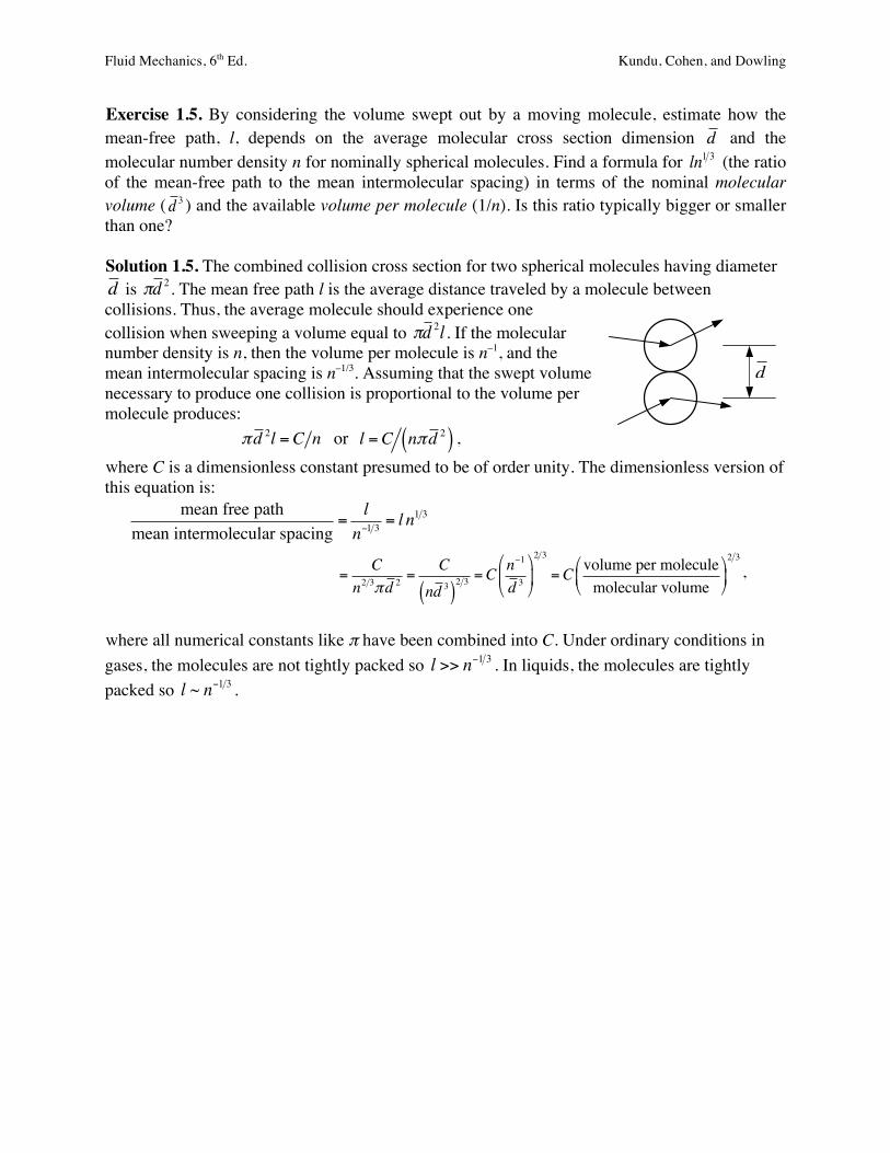
Exercise 1.5. By considering the volume swept out by a moving molecule, estimate how the mean-free path, l, depends on the average molecular cross section dimension d and the molecular number density n for nominally spherical molecules. Find a formula for (the ratio of the mean-free path to the mean intermolecular spacing) in terms of the nominal molecular volume ( ) and the available volume per molecule (1/n). Is this ratio typically bigger or smaller than one? Solution 1.5. The combined collision cross section for two spherical molecules having diameter
€
d is
€
πd 2. The mean free path l is the average distance traveled by a molecule between collisions. Thus, the average molecule should experience one collision when sweeping a volume equal to
€
πd 2l . If the molecular number density is n, then the volume per molecule is n–1, and the mean intermolecular spacing is n–1/3. Assuming that the swept volume necessary to produce one collision is proportional to the volume per molecule produces:
πd 2l =C n or l =C nπd 2( ) , where C is a dimensionless constant presumed to be of order unity. The dimensionless version of this equation is:
mean free pathmean intermolecular spacing
=l
n−1 3 = l n1 3
= Cn2 3πd 2 =
Cnd 3( )
2 3 =Cn−1
d 3
"
#$
%
&'
2 3
=C volume per moleculemolecular volume
"
#$
%
&'
2 3
,
where all numerical constants like π have been combined into C. Under ordinary conditions in gases, the molecules are not tightly packed so l >> n−1 3 . In liquids, the molecules are tightly packed so l ~ n−1 3 .
ln1 3
d 3
€
d

Fluid Mechanics, 6th Ed. Kundu, Cohen, and Dowling
Exercise 1.6. Compute the average relative speed, vr , between molecules in a gas using the Maxwell speed distribution f given by (1.4) via the following steps. a) If u and v are the velocities of two molecules then their relative velocity is: vr = u – v. If the angle between u and v is θ, show that the relative speed is: vr = |vr| = u2 + v2 − 2uvcosθ where u = |u|, and v = |v|. b) The averaging of vr necessary to determine vr must include all possible values of the two speeds (u and v) and all possible angles θ. Therefore, start from:
vr =1
2n2 vr f (u)all u,v,θ∫ f (v)sinθdθdvdu ,
and note that vr is unchanged by exchange of u and v, to reach:
vr =1n2
u2 + v2 − 2uvcosθθ=0
π
∫v=u
∞
∫u=0
∞
∫ sinθ f (u) f (v)dθdvdu
c) Note that vr must always be positive and perform the integrations, starting with the angular one, to find:
vr =13n2
2u3 + 6uv2
uvv=u
∞
∫u=0
∞
∫ f (u) f (v)dvdu = 16kBTπ
#
$%
&
'(1 2
= 2 v .
Solution 1.6. a) Compute the dot produce of vr with itself:
vr2= vr ⋅vr = (u− v) ⋅ (u− v) = u ⋅u− 2u ⋅v+ v ⋅v = u
2 − 2uvcosθ + v2 .
Take the square root to find: |vr| = u2 + v2 − 2uvcosθ . b) The average relative speed must account for all possible molecular speeds and all possible angles between the two molecules. [The coefficient 1/2 appears in the first equality below because the probability density function of for the angle θ in the interval 0 ≤ θ ≤ π is (1/2)sinθ.]
vr =1
2n2 vr f (u)all u,v,θ∫ f (v)sinθdθdvdu
= 12n2 u2 + v2 − 2uvcosθ f (u)
all u,v,θ∫ f (v)sinθdθdvdu
= 12n2 u2 + v2 − 2uvcosθ
θ=0
π
∫v=0
∞
∫u=0
∞
∫ sinθ f (u) f (v)dθdvdu.
In u-v coordinates, the integration domain covers the first quadrant, and the integrand is unchanged when u and v are swapped. Thus, the u-v integration can be completed above the line u = v if the final result is doubled. Thus,
vr =1n2
u2 + v2 − 2uvcosθθ=0
π
∫v=u
∞
∫u=0
∞
∫ sinθ f (u) f (v)dθdvdu .
Now tackle the angular integration, by setting β = u2 + v2 − 2uvcosθ so that dβ = +2uvsinθdθ . This leads to
vr =1n2
β1 2
β=(v−u)2
(v+u)2
∫v=u
∞
∫u=0
∞
∫ dβ2uv
f (u) f (v)dvdu , u!
v! dv!
du!
u = v!

Fluid Mechanics, 6th Ed. Kundu, Cohen, and Dowling
and the β-integration can be performed:
vr =12n2
23β 3 2( )(v−u)2
(v+u)2
v=u
∞
∫u=0
∞
∫ f (u)u
f (v)v
dvdu = 13n2
(v+u)3 − (v−u)3( )v=u
∞
∫u=0
∞
∫ f (u)u
f (v)v
dvdu .
Expand the cubic terms, simplify the integrand, and prepare to evaluate the v-integration:
vr =1
3n2 2u3 + 6uv2( )v=u
∞
∫u=0
∞
∫ f (v)v
dv f (u)u
du
= 13n
2u3 + 6uv2( )v=u
∞
∫u=0
∞
∫ 4πv
m2πkBT#
$%
&
'(
3 2
v2 exp −mv2
2kBT*+,
-./dv f (u)
udu.
Use the variable substitution: α = mv2/2kBT so that dα = mvdv/kBT, which reduces the v-integration to:
vr =13n
2u3 + 6u kBTm
α!
"#
$
%&
mu2 kBT
∞
∫u=0
∞
∫ 4π m2πkBT!
"#
$
%&
3 2
exp −α{ }kBTm
dα f (u)u
du
= 23n
m2πkBT!
"#
$
%&
1 2
2u3 + 6u kBTm
α!
"#
$
%&
mu2 kBT
∞
∫u=0
∞
∫ e−αdα f (u)u
du
= 23n
m2πkBT!
"#
$
%&
1 2
−2u3e−α + 6u kBTm
−αe−α − e−α( )!
"#
$
%&mu2 kBT
∞
u=0
∞
∫ f (u)u
du
= 23n
m2πkBT!
"#
$
%&
1 2
8u3 +12u kBTm
!
"#
$
%&
u=0
∞
∫ exp −mu2
2kBT!
"#
$
%&f (u)u
du.
The final u-integration may be completed by substituting in for f(u) and using the variable substitution γ = u m kBT( )1 2 .
vr =13
2mπkBT!
"#
$
%&
1 2
8 kBTm
!
"#
$
%&
3 2
γ 3 +12 kBTm
!
"#
$
%&
3 2
γ!
"##
$
%&&
0
∞
∫ 4π m2πkBT!
"#
$
%&
3 2kBTm
!
"#
$
%&γ exp −γ 2( )dγ
= 23π
kBTm
!
"#
$
%&
1 2
8γ 4 +12γ 2( )0
∞
∫ exp −γ 2( )dγ = 23π
kBTm
!
"#
$
%&
1 2
8 38
π +12 14
π!
"#
$
%&
= 4π
kBTm
!
"#
$
%&
1 2
=16kBTπm
!
"#
$
%&
1 2
= 2v
Here, v is the mean molecular speed from (1.5).

Fluid Mechanics, 6th Ed. Kundu, Cohen, and Dowling
Exercise 1.7. In a gas, the molecular momentum flux (MFij) in the j-coordinate direction that crosses a flat surface of unit area with coordinate normal direction i is:
MFij =1V
mvivj f (v)d3vall v∫∫∫ where f(v) is the Maxwell velocity distribution (1.1). For a perfect
gas that is not moving on average (i.e., u = 0), show that MFij = p (the pressure), when i = j, and that MFij = 0, when i ≠ j. Solution 1.7. Start from the given equation using the Maxwell distribution:
MFij =1V
mvivj f (v)d3vall u∫∫∫ =
nmV
m2πkBT"
#$
%
&'
3 2
vivj−∞
+∞
∫−∞
+∞
∫−∞
+∞
∫ exp −m
2kBTv1
2 + v22 + v3
2( )*+,
-./dv1dv2dv3
and first consider i = j = 1, and recognize ρ = nm/V as the gas density, as in (1.28).
MF11 = ρm
2πkBT!
"#
$
%&
3 2
u12
−∞
+∞
∫−∞
+∞
∫−∞
+∞
∫ exp −m2kBT
v12 + v2
2 + v32( )
*+,
-./dv1dv2dv3
= ρ
m2πkBT!
"#
$
%&
3 2
v12 exp −
mv12
2kBT()*
+,-dv1
−∞
+∞
∫ exp −mv2
2
2kBT()*
+,-dv2
−∞
+∞
∫ exp −mv3
2
2kBT()*
+,-−∞
+∞
∫ dv3
The first integral is equal to 2kBT m( )3 2 π 2( ) while the second two integrals are each equal to
2πkBT m( )1 2 . Thus:
MF11 = ρm
2πkBT!
"#
$
%&
3 22kBTm
!
"#
$
%&3 2
π2
2πkBTm
!
"#
$
%&1 2 2πkBT
m!
"#
$
%&1 2
= ρkBTm
= ρRT = p
where kB/m = R from (1.28). This analysis may be repeated with i = j = 2, and i = j = 3 to find: MF22 = MF33 = p, as well. Now consider the case i ≠ j. First note that MFij = MFji because the velocity product under the triple integral may be written in either order vivj = vjvi, so there are only three cases of interest. Start with i = 1, and j = 2 to find:
MF12 = ρm
2πkBT!
"#
$
%&
3 2
v1v2−∞
+∞
∫−∞
+∞
∫−∞
+∞
∫ exp −m2kBT
v12 + v2
2 + v32( )
*+,
-./dv1dv2dv3
= ρ
m2πkBT!
"#
$
%&
3 2
v1 exp −mv1
2
2kBT()*
+,-dv1
−∞
+∞
∫ v2 exp −mv2
2
2kBT()*
+,-dv2
−∞
+∞
∫ exp −mv3
2
2kBT()*
+,-−∞
+∞
∫ dv3
Here we need only consider the first integral. The integrand of this integral is an odd function because it is product of an odd function, v1, and an even function, exp −mv1
2 2kBT{ } . The integral of an odd function on an even interval [–∞,+∞] is zero, so MF12 = 0. And, this analysis may be repeated for i = 1 and j = 3, and i = 2 and j = 3 to find MF13 = MF23 = 0.

Fluid Mechanics, 6th Ed. Kundu, Cohen, and Dowling
Exercise 1.8. Consider the viscous flow in a channel of width 2b. The channel is aligned in the x-direction, and the velocity u in the x-direction at a distance y from the channel centerline is given by the parabolic distribution
€
u(y) =U0 1− y b( )2[ ]. Calculate the shear stress τ as a
function y, µ, b, and Uo. What is the shear stress at y = 0?
Solution 1.8. Start from (1.3):
€
τ = µdudy
= µddyUo 1−
yb$
% & '
( ) 2*
+ ,
-
. / = –2µUo
yb2
. At y = 0 (the location of
maximum velocity) τ = 0. At At y = ±b (the locations of zero velocity),
€
τ = 2µUo b .
Fluid Mechanics, 6th Ed. Kundu, Cohen, and Dowling
Exercise 1.9. Hydroplaning occurs on wet roadways when sudden braking causes a moving vehicle’s tires to stop turning when the tires are separated from the road surface by a thin film of water. When hydroplaning occurs the vehicle may slide a significant distance before the film breaks down and the tires again contact the road. For simplicity, consider a hypothetical version of this scenario where the water film is somehow maintained until the vehicle comes to rest. a) Develop a formula for the friction force delivered to a vehicle of mass M and tire-contact area A that is moving at speed u on a water film with constant thickness h and viscosity µ. b) Using Newton’s second law, derive a formula for the hypothetical sliding distance D traveled by a vehicle that started hydroplaning at speed Uo c) Evaluate this hypothetical distance for M = 1200 kg, A = 0.1 m2, Uo = 20 m/s, h = 0.1 mm, and µ = 0.001 kgm–1s–1. Compare this to the dry-pavement stopping distance assuming a tire-road coefficient of kinetic friction of 0.8. Solution 1.9. a) Assume that viscous friction from the water layer transmitted to the tires is the only force on the sliding vehicle. Here viscous shear stress at any time will be µu(t)/h, where u(t) is the vehicle's speed. Thus, the friction force will be Aµu(t)/h.
b) The friction force will oppose the motion so Newton’s second law implies: M dudt= −Aµ u
h.
This equation is readily integrated to find an exponential solution: u(t) =Uo exp −Aµt Mh( ) , where the initial condition, u(0) = Uo, has been used to evaluate the constant of integration. The distance traveled at time t can be found from integrating the velocity:
x(t) = u( !t )d !to
t∫ =Uo exp −Aµ !t Mh( )d !t
o
t∫ = UoMh Aµ( ) 1− exp −Aµt Mh( )$% &' .
The total sliding distance occurs for large times where the exponential term will be negligible so: D =UoMh Aµ
c) For M = 1200 kg, A = 0.1 m2, Uo = 20 m/s, h = 0.1 mm, and µ = 0.001 kgm–1s–1, the stopping distance is: D = (20)(1200)(10–4)/(0.1)(0.001) = 24 km! This is an impressively long distance and highlights the dangers of driving quickly on water covered roads. For comparison, the friction force on dry pavement will be –0.8Mg, which leads to a vehicle velocity of: u(t) =Uo − 0.8gt , and a distance traveled of x(t) =Uot − 0.4gt
2 . The vehicle stops when u = 0, and this occurs at t = Uo/(0.8g), so the stopping distance is
D =UoUo
0.8g!
"#
$
%&− 0.4g
Uo
0.8g!
"#
$
%&
2
=Uo2
1.6g,
which is equal to 25.5 m for the conditions given. (This is nearly three orders of magnitude less than the estimated stopping distance for hydroplaning.)

Fluid Mechanics, 6th Ed. Kundu, Cohen, and Dowling
Exercise 1.10. Estimate the height to which water at 20°C will rise in a capillary glass tube 3 mm in diameter that is exposed to the atmosphere. For water in contact with glass the contact angle is nearly 0°. At 20°C, the surface tension of a water-air interface is σ = 0.073 N/m. Solution 1.10. Start from the result of Example 1.4.
h = 2σ cosαρgR
=2(0.073N /m)cos(0°)
(103kg /m3)(9.81m / s2 )(1.5×10⁻³m)= 9.92mm
Fluid Mechanics, 6th Ed. Kundu, Cohen, and Dowling
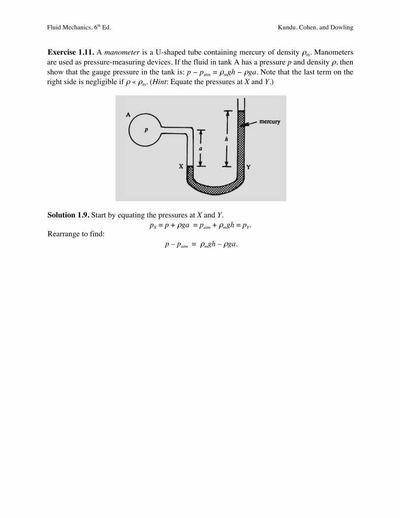
Exercise 1.11. A manometer is a U-shaped tube containing mercury of density ρm. Manometers are used as pressure-measuring devices. If the fluid in tank A has a pressure p and density ρ, then show that the gauge pressure in the tank is: p − patm = ρmgh − ρga. Note that the last term on the right side is negligible if ρ « ρm. (Hint: Equate the pressures at X and Y.)
Solution 1.9. Start by equating the pressures at X and Y.
pX = p + ρga = patm + ρmgh = pY. Rearrange to find:
p – patm = ρmgh – ρga.
Fluid Mechanics, 6th Ed. Kundu, Cohen, and Dowling
Exercise 1.12. Prove that if e(T, υ) = e(T) only and if h(T, p) = h(T) only, then the (thermal) equation of state is (1.28) or pυ = kT, where k is constant. Solution 1.12. Start with the first equation of (1.24): de = Tds – pdυ, and rearrange it:
€
ds =1Tde +
pTdυ =
∂s∂e$
% &
'
( ) υ
de +∂s∂υ
$
% &
'
( ) e
dυ ,
where the second equality holds assuming the entropy depends on e and υ. Here we see that:
€
1T
=∂s∂e#
$ %
&
' ( υ
, and
€
pT
=∂s∂υ
$
% &
'
( ) e
.
Equality of the crossed second derivatives of s,
€
∂∂υ
∂s∂e$
% &
'
( ) υ
$
% &
'
( ) e
=∂∂e
∂s∂υ
$
% &
'
( ) e
$
% &
'
( ) υ
, implies:
€
∂ 1 T( )∂υ
$
% &
'
( ) e
=∂ p T( )∂e
$
% &
'
( ) υ
.
However, if e depends only on T, then (∂/∂υ)e = (∂/∂υ)T, thus
€
∂ 1 T( )∂υ
$
% &
'
( ) e
=∂ 1 T( )∂υ
$
% &
'
( ) T
= 0 , so
€
∂ p T( )∂e
#
$ %
&
' ( υ
= 0 , which can be integrated to find: p/T = f1(υ), where f1 is an undetermined function.
Now repeat this procedure using the second equation of (1.24), dh = Tds + υdp.
€
ds =1Tdh − υ
Tdp =
∂s∂h%
& '
(
) * p
dh +∂s∂p%
& '
(
) * h
dp.
Here equality of the coefficients of the differentials implies:
€
1T
=∂s∂h#
$ %
&
' ( p, and
€
−υT
=∂s∂p%
& '
(
) * h
.
So, equality of the crossed second derivatives implies:
€
∂ 1 T( )∂p
#
$ %
&
' ( h
= −∂ υ T( )∂h
#
$ %
&
' ( p
. Yet, if h depends
only on T, then (∂/∂p)h = (∂/∂p)T, thus
€
∂ 1 T( )∂p
#
$ %
&
' ( h
=∂ 1 T( )∂p
#
$ %
&
' ( T
= 0, so
€
−∂ υ T( )∂h
%
& '
(
) * p
= 0 , which can
be integrated to find: υ/T = f2(p), where f2 is an undetermined function. Collecting the two results involving f1 and f2, and solving for T produces:
€
pf1(υ)
= T =υf2(p)
or
€
pf2(p) =υf1(υ) = k ,
where k must be is a constant since p and υ are independent thermodynamic variables. Eliminating f1 or f2 from either equation on the left, produces pυ = kT. And finally, using both versions of (1.24) we can write: dh – de = υdp + pdυ = d(pυ). When e and h only depend on T, then dh = cpdT and de = cvdT, so
dh – de = (cp – cv)dT = d(pυ) = kdT , thus k = cp – cv = R, where R is the gas constant. Thus, the final result is the perfect gas law: p = kT/υ = ρRT.

Fluid Mechanics, 6th Ed. Kundu, Cohen, and Dowling
Exercise 1.13. Starting from the property relationships (1.24) prove (1.31) and (1.32) for a reversible adiabatic process involving a perfect gas when the specific heats cp and cv are constant. Solution 1.13. For an isentropic process: de = Tds – pdυ = –pdυ, and dh = Tds + υdp = +υdp. Equations (1.31) and (1.32) apply to a perfect gas so the definition of the specific heat capacities (1.20), and (1.21) for a perfect gas, dh = cpdT, and de = cvdT , can be used to form the ratio dh/de:
dhde
=cpdTcvdT
=cpcv= γ = −
υdppdυ
or
€
−γdυυ
= γdρρ
=dpp
.
The final equality integrates to: ln(p) = γln(ρ) + const which can be exponentiated to find: p = const.ργ,
which is (1.31). The constant may be evaluated at a reference condition po and ρo to find:
€
p po = ρ ρo( )γ and this may be inverted to put the density ratio on the left
€
ρ ρo = p po( )1 γ , which is the second equation of (1.32). The remaining relationship involving the temperature is found by using the perfect gas law, p = ρRT, to eliminate ρ = p/RT:
€
ρρo
=p RTpo RTo
=pTopoT
=ppo
#
$ %
&
' (
1 γ
or
€
TTo
=ppo
ppo
"
# $
%
& '
−1 γ
=ppo
"
# $
%
& '
(γ −1) γ
,
which is the first equation of (1.32).

Fluid Mechanics, 6th Ed. Kundu, Cohen, and Dowling
Exercise 1.14. A cylinder contains 2 kg of air at 50°C and a pressure of 3 bars. The air is compressed until its pressure rises to 8 bars. What is the initial volume? Find the final volume for both isothermal compression and isentropic compression. Solution 1.14. Use the perfect gas law but explicitly separate the mass M of the air and the volume V it occupies via the substitution ρ = M/V:
p = ρRT = (M/V)RT. Solve for V at the initial time:
Vi = initial volume = MRT/pi = (2 kg)(287 m2/s2K)(273 + 50°)/(300 kPa) = 0.618 m3. For an isothermal process:
Vf = final volume = MRT/pf = (2 kg)(287 m2/s2K)(273 + 50°)/(800 kPa) = 0.232 m3. For an isentropic process:
Vf =Vi pi pf( )1 γ= 0.618m3 300kPa 800kPa( )1 1.4 = 0.307m3 .

Fluid Mechanics, 6th Ed. Kundu, Cohen, and Dowling
Exercise 1.15. Derive (1.35) starting from Figure 1.9 and the discussion at the beginning of Section 1.10. Solution 1.15. Take the z axis vertical, and consider a small fluid element δm of fluid having volume δV that starts at height z0 in a stratified fluid medium having a vertical density profile = ρ(z), and a vertical pressure profile p(z). Without any vertical displacement, the small mass and its volume are related by δm = ρ(z0)δV. If the small mass is displaced vertically a small distance ζ via an isentropic process, its density will change isentropically according to:
€
ρa (z0 + ζ ) = ρ(z0) + dρa dz( )ζ + ... where dρa/dz is the isentropic density gradient at z0. For a constant δm, the volume of the fluid element will be:
€
δV =δmρa
=δm
ρ(z0) + dρa dz( )ζ + ...=
δmρ(z0)
1− 1ρ(z0)
dρadz
ζ + ...&
' (
)
* +
The background density at z0 + ζ is:
€
ρ(z0 + ζ ) = ρ(z0) + dρ dz( )ζ + ... If g is the acceleration of gravity, the (upward) buoyant force on the element at the vertically displaced location will be gρ(z0 + ζ)δV, while the (downward) weight of the fluid element at any vertical location is gδm. Thus, a vertical application Newton's second law implies:
€
δm d2ζdt 2
= +gρ(z0 + ζ )δV − gδm = g ρ(z0) + dρ dz( )ζ + ...( ) δmρ(z0)
1− 1ρ(z0)
dρadz
ζ + ...&
' (
)
* + − gδm ,
where the second equality follows from substituting for ρ(z0 + ζ) and δV from the above equations. Multiplying out the terms in (,)-parentheses and dropping second order terms produces:
€
δm d2ζdt 2
= gδm +gδmρ(z0)
dρdzζ −
gδmρ(z0)
dρadz
ζ + ...− gδm ≅gδmρ(z0)
dρdz
−dρadz
'
( )
*
+ , ζ
Dividing by δm and moving all the terms to the right side of the equation produces:
€
d2ζdt 2
−g
ρ(z0)dρdz
−dρadz
%
& '
(
) * ζ = 0
Thus, for oscillatory motion at frequency N, we must have
€
N 2 = −g
ρ(z0)dρdz
−dρadz
$
% &
'
( ) ,
which is (1.35).

Fluid Mechanics, 6th Ed. Kundu, Cohen, and Dowling
Exercise 1.16. Starting with the hydrostatic pressure law (1.14), prove (1.36) without using perfect gas relationships. Solution 1.16. The adiabatic temperature gradient dTa/dz, can be written terms of the pressure gradient:
€
dTadz
=∂T∂p#
$ %
&
' ( s
dpdz
= −gρ ∂T∂p#
$ %
&
' ( s
where the hydrostatic law dp/dz = –ρg has been used to reach the second equality. Here, the final partial derivative can be exchanged for one involving υ = 1/ρ and s, by considering:
€
dh =∂h∂s#
$ %
&
' ( p
ds+∂h∂p#
$ %
&
' ( s
dp = Tds+υdp .
Equality of the crossed second derivatives of h,
€
∂∂p
∂h∂s#
$ %
&
' ( p
#
$ %
&
' ( s
=∂∂s
∂h∂p#
$ %
&
' ( s
#
$ %
&
' ( p
, implies:
€
∂T∂p#
$ %
&
' ( s
=∂υ∂s#
$ %
&
' ( p
=∂υ∂T#
$ %
&
' ( p
∂T∂s#
$ %
&
' ( p
=∂υ∂T#
$ %
&
' ( p
∂s∂T#
$ %
&
' ( p
,
where the second two equalities are mathematical manipulations that allow the introduction of
€
α = −1ρ∂ρ∂T&
' (
)
* + p
= ρ∂υ∂T&
' (
)
* + p, and cp =
∂h∂T!
"#
$
%&p
= T ∂s∂T!
"#
$
%&p
.
Thus, dTadz
= −gρ ∂T∂ p"
#$
%
&'s
= −gρ ∂υ∂T"
#$
%
&'p
∂s∂T"
#$
%
&'p
= −gαcpT"
#$
%
&'= −
gαTcp
.

Fluid Mechanics, 6th Ed. Kundu, Cohen, and Dowling
Exercise 1.17. Assume that the temperature of the atmosphere varies with height z as T = T0 +
Kz where K is a constant. Show that the pressure varies with height as p = p0T0
T0 +Kz!
"#
$
%&
g KR
where
g is the acceleration of gravity and R is the gas constant for the atmospheric gas. Solution 1.17. Start with the hydrostatic and perfect gas laws, dp/dz = –ρg, and p = ρRT, eliminate the density, and substitute in the given temperature profile to find:
€
dpdz
= −ρg = −pRT
g = −p
R(T0 + Kz)g or
€
dpp
= −gR
dz(T0 + Kz)
.
The final form may be integrated to find:
€
ln p = −gRK
ln T0 + Kz( ) + const.
At z = 0, the pressure must be p0, therefore:
€
ln p0 = −gRK
ln T0( ) + const.
Subtracting this from the equation above and invoking the properties of logarithms produces:
€
ln pp0
"
# $
%
& ' = −
gRK
ln T0 + KzT0
"
# $
%
& '
Exponentiating produces:
€
pp0= T0 + Kz
T0
"
# $
%
& '
−g/KR
, which is the same as:
€
p = p0T0
T0 + Kz"
# $
%
& '
g/KR
.

Fluid Mechanics, 6th Ed. Kundu, Cohen, and Dowling
Exercise 1.18. Suppose the atmospheric temperature varies according to: T = 15 − 0.001z, where T is in degrees Celsius and height z is in meters. Is this atmosphere stable? Solution 1.18. Compute the temperature gradient:
€
dTdz
=ddz(15 − 0.001z) = −0.001°C
m= −1.0 °C
km.
For air in the earth's gravitational field, the adiabatic temperature gradient is: dTadz
= −gαTcp
=(9.81m / s2 )(1 /T )T1004m2 / s2°C
= −9.8 °Ckm
.
Thus, the given temperature profile is stable because the magnitude of its gradient is less than the magnitude of the adiabatic temperature gradient.

Fluid Mechanics, 6th Ed. Kundu, Cohen, and Dowling
Exercise 1.19. A hemispherical bowl with inner radius r containing a liquid with density ρ is inverted on a smooth flat surface. Gravity with acceleration g acts downward. Determine the weight W of the bowl necessary to prevent the liquid from escaping. Consider two cases: a) the pressure around the rim of the bowl where it meets the plate is atmospheric, and b) the pressure at the highest point of the bowl’s interior is atmospheric. c) Investigate which case applies via a simple experiment. Completely fill an ordinary soup bowl with water and concentrically cover it with an ordinary dinner plate. While holding the bowl and plate together, quickly invert the water-bowl-plate combination, set it on the level surface at the bottom of a kitchen sink, and let go. Does the water escape? If no water escapes after release, hold onto the bowl only and try to lift the water-bowl-plate combination a few centimeters off the bottom of the sink. Does the plate remain in contact with the bowl? Do your answers to the first two parts of this problem help explain your observations? Solution 1.19. a) When the pressure around the inverted bowl's rim is atmospheric, the surface does not support the weight of the liquid and any increase in elevation above the rim must produce a lower pressure in the liquid. In this case the weight of the liquid is supported by a reduced pressure on the interior of the bowl. Thus the vertical force Fz that the bowl applies to the surface is negative and includes its own weight, W, and the weight of the liquid 2 3( )πr3ρg :
Fz = −W − 2 3( )πr3ρg . So, for Fz to reach zero, the point of bowl lift-off, W must be negative! This implies that the bowl will adhere to the surface and will not separate unless it's pulled upward. This finding concerning the pressure force on the bowl can be reached via a more traditional hydrostatic calculation using spherical coordinates (see Appendix B.5). The net vertical pressure force on the inverted bowl will be:
Fz,pressure = 2π (p− po ) er ⋅ ez( )r2 sinθ dθθ=0
π 2
∫ = 2πr2 (p− po )cosθ sinθ dθθ=0
π 2
∫ ,
where p is the pressure inside the bowl and po is the pressure outside the bowl (atmospheric pressure). Here θ is the polar angle (θ = 0 defines the positive z-axis). In this coordinate system z = rcosθ, and the pressure inside and outside the bowl must match when z = 0, so p – po = –ρgz = –ρgrcosθ, so
Fz,pressure = −ρg2πr3 cos2θ sinθ dθθ=0
π 2
∫ = −2π3r3ρg .
So, the bowl's "weight" must be less than − 2 3( )πr3ρg to keep the liquid trapped. b) In this case the pressure force on the bowl is different because atmospheric pressure is reached at the inside top of the bowl. In this case, p – po = –ρg(z – r), and the vertical pressure force calculation looks like:
Fz,pressure = 2πr2 (p− po )cosθ sinθ dθθ=0
π 2
∫ = −ρg2πr3 (cosθ −1)cosθ sinθ dθθ=0
π 2
∫
= 13ρgπr3.
So, the static force balance for the bowl is: Fz = −W + 1 3( )πr3ρg . Thus, the bowl's weight must be more than 1 3( )πr3ρg to keep the liquid trapped.

Fluid Mechanics, 6th Ed. Kundu, Cohen, and Dowling
c) Interestingly, even though a little bit of water may escape from underneath the inverted bowl, nearly all the water remains trapped under the bowl when the bowl-plate combination is released, and the inverted bowl does adhere to the plate when it is lifted. These observations closely match the part a) answer, so it is the physically meaningful one.

Fluid Mechanics, 6th Ed. Kundu, Cohen, and Dowling
Exercise 1.20. Consider the case of a pure gas planet where the hydrostatic law is: dp dz = −ρ(z)Gm(z) z2 , where G is the gravitational constant and m(z) = 4π ρ(ζ )ζ 2
o
z∫ dζ is the
planetary mass up to distance z from the center of the planet. If the planetary gas is perfect with gas constant R, determine ρ(z) and p(z) if this atmosphere is isothermal at temperature T. Are these vertical profiles of ρ and p valid as z increases without bound? Solution 1.20. Start with the given relationship for m(z), differentiate it with respect to z, and use the perfect gas law, p = ρRT to replace the ρ with p.
€
dmdz
=ddz
4π ρ(ζ )ζ 2dζ0
z
∫&
' (
)
* + = 4πz2ρ(z) = 4πz2 p(z)
RT.
Now use this and the hydrostatic law to obtain a differential equation for m(z), dpdz
= −ρ(z)Gm(z)z2
→ddz
RT4π z2
dmdz
#
$%
&
'(= −
14π z2
dmdz
#
$%
&
'(Gm(z)z2
.
After recognizing T as a constant, the nonlinear second-order differential equation for m(z) simplifies to:
€
RTG
ddz
1z2dmdz
"
# $
%
& ' = −
1z4m dmdz
.
This equation can be solved by assuming a power law: m(z) = Azn. When substituted in, this trial solution produces:
€
RTG
ddz
z−2Anzn−1( ) =RTG
n − 3( )Anzn−4 = −z−4A2nz2n−1.
Matching exponents of z across the last equality produces: n – 4 = 2n – 5, and this requires n = 1. For this value of n, the remainder of the equation is:
€
RTG
−2( )Az−3 = −z−4A2z1 , which reduces to:
€
A = 2 RTG
.
Thus, we have m(z) = 2RTz/G, and this leads to:
€
ρ(z) =2RTG
14πz2
, and
€
p(z) =2R2T 2
G14πz2
.
Unfortunately, these profiles are not valid as z increases without bound, because this leads to an unbounded planetary mass.

Fluid Mechanics, 6th Ed. Kundu, Cohen, and Dowling
Exercise 1.21. Consider a gas atmosphere with pressure distribution p(z) = p0 1− (2 /π )tan
−1(z /H )( ) where z is the vertical coordinate and H is a constant length scale. a) Determine the vertical profile of ρ from (1.14) b) Determine N2 from (1.35) as function of vertical distance, z. c) Near the ground where z << H, this atmosphere is unstable, but it is stable at greater heights where z >> H. Specify the value of z/H above which this atmosphere is stable. Solution 1.21. a) Start from (1.14):
dpdz
= −ρg = −po2π
11+ (z /H )2
1H
so ρ(z) = 2poπgH
11+ (z /H )2
.
b) First determine dρ/dz: dρdz
= −2poπgH
11+ (z /H )2( )
22zH 2 = −ρ
2z H 2
1+ (z /H )2"
#$
%
&' .
Determine the local adiabatic density gradient by expanding (1.31) for small vertical displacement ζ that leads to an adiabatic density change:
p(z)+ζ dp dz( )+...p(z)
=ρ(z)+ζ dρa dz( )+...
ρ(z)!
"#
$
%&
γ
or 1+ ζpdpdz+... = 1+ ζ
ρdρadz
+...!
"#
$
%&
γ
.
For small ζ, expand the final term and cancel the leading 1's, to find: 1pdpdz
=γρdρadz
= −ρgp
, thus: dρadz
= −ρ2gγ p
.
where the second equality follows from (1.14). Now use (1.35)
N 2 = −gρ
dρdz
−dρadz
"
#$
%
&'= −
gρ−ρ
2z H 2
1+ (z /H )2
"
#$
%
&'+
ρ2gγ p
"
#$
%
&'= g 2z H 2
1+ (z /H )2 −ρgγ p
"
#$
%
&'
= g 2z H 2
1+ (z /H )2 −2
γπH 1− (2 /π )tan−1(z /H )( )1
1+ (z /H )2
"
#$$
%
&''
= 2g H1+ (z /H )2
zH−
1γπ 1− (2 /π )tan−1(z /H )( )
"
#$$
%
&''
.
c) In the limit as z H→ 0 , the terms inside the big parentheses go to –1/γπ, which is negative, so N2 is negative, and this indicates an unstable atmosphere. In the limit as z H→∞ , both terms inside the big parentheses become large, but the first one is larger so N2 is positive, and this indicates a stable atmosphere. The boundary between the two regimes occurs when the terms inside the big parentheses sum to zero. This condition leads to an implicit equation for z/H:
zH−
1γπ 1− (2 /π )tan−1(z /H )( )
= 0 , or γ zH
π − 2 tan−1 zH"
#$
%
&'
"
#$
%
&'=1 ,
which has numerical solution z/H = 0.274 when γ = 1.4.

Fluid Mechanics, 6th Ed. Kundu, Cohen, and Dowling
Exercise 1.22. Consider a heat-insulated enclosure that is separated into two compartments of volumes V1 and V2, containing perfect gases with pressures and temperatures of p1 and p2, and T1 and T2, respectively. The compartments are separated by an impermeable membrane that conducts heat (but not mass). Calculate the final steady-state temperature assuming each gas has constant specific heats. Solution 1.22. Since no work is done and no heat is transferred out of the enclosure, the final energy Ef is the sum of the energies, E1 and E2, in the two compartments.
E1 + E2 = Ef implies ρ1V1cv1T1 + ρ2V2cv2T2 = (ρ1V1cv1 + ρ2V2cv2)Tf, where the cv's are the specific heats at constant volume for the two gases. The perfect gas law can be used to find the densities: ρ1 = p1/R1T1 and ρ2 = p2/R2T2, so
p1V1cv1/R1 + p2V2cv2/R2 = (p1V1cv1/R1T1 + p2V2cv2/R2T2)Tf. A little more simplification is possible, cv1/R1 = 1/(γ1 – 1) and cv2/R1 = 1/(γ2 – 1). Thus, the final temperature is:
€
Tf =p1V1 (γ1 −1) + p2V2 (γ 2 −1)
p1V1 (γ1 −1)T1[ ] + p2V2 (γ 2 −1)T2[ ].

Fluid Mechanics, 6th Ed. Kundu, Cohen, and Dowling
Exercise 1.23. Consider the initial state of an enclosure with two compartments as described in Exercise 1.22. At t = 0, the membrane is broken and the gases are mixed. Calculate the final temperature. Solution 1.23. No heat is transferred out of the enclosure and the work done by either gas is delivered to the other so the total energy is unchanged. First consider the energy of either gas at temperature T, and pressure P in a container of volume V. The energy E of this gas will be:
E = ρVcvT = (p/RT)VcvT = pV(cv/R) = pV/(γ – 1). where γ is the ratio of specific heats. For the problem at hand the final energy Ef will be the sum of the gas energies, E1 and E2, in the two compartments. Using the above formula:
€
E f = p1V1 (γ1 −1) + p2V2 (γ 2 −1) . Now consider the mixture. The final volume and temperature for both gases is V1+V2, and Tf. However, from Dalton's law of partial pressures, the final pressure of the mixture pf can be considered a sum of the final partial pressures of gases "1" and "2", p1f and p2f:
pf = p1f + p2f. Thus, the final energy of the mixture is a sum involving each gases' partial pressure and the total volume:
€
E f = p1 f (V1 +V2) (γ1 −1) + p2 f (V1 +V2) (γ 2 −1). However, the perfect gas law implies: p1f(V1+V2) = n1RuTf, and p2f(V1+V2) = n2RuTf where n1 and n2 are the mole numbers of gases "1" and "2", and Ru is the universal gas constant. The mole numbers are obtained from:
n1 = p1V1/RuT1, and n2 = p2V2/RuT2, Thus, final energy determined from the mixture is:
€
E f =n1RuTfγ1 −1
+n2RuTfγ1 −1
=p1V1RuT1
$
% &
'
( ) RuTfγ1 −1
+p2V2RuT2
$
% &
'
( ) RuTfγ 2 −1
=p1V1T1
$
% &
'
( ) Tfγ1 −1
+p2V2T2
$
% &
'
( ) Tfγ 2 −1
.
Equating this and the first relationship for Ef above then produces:
€
Tf =p1V1 (γ1 −1) + p2V2 (γ 2 −1)
p1V1 (γ1 −1)T1[ ] + p2V2 (γ 2 −1)T2[ ].

Fluid Mechanics, 6th Ed. Kundu, Cohen, and Dowling
Exercise 1.24. A heavy piston of weight W is dropped onto a thermally insulated cylinder of cross-sectional area A containing a perfect gas of constant specific heats, and initially having the external pressure p1, temperature T1, and volume V1. After some oscillations, the piston reaches an equilibrium position L meters below the equilibrium position of a weightless piston. Find L. Is there an entropy increase? Solution 1.24. From the first law of thermodynamics, with Q = 0, ΔE = Work = (W + p1A)L. For a total mass m of a perfect gas with constant specific heats, E = mcvT so ΔE = E2 – E1 = mcv(T2 – T1) = (W + p1A)L. Then T2 = T1 + (W + p1A)L/mcv. Also, for a perfect gas, PV/T = constant so p1V1/T1 = p2V2/T2. For the cylinder, V2 = V1 – AL, and p2 = p1 + W/A. Therefore:
p1V1T1
=(p1 +W A)(V1 − AL)T1 + (W + p1A)L mcv
.
Here, m = p1V1/RT1 so mcv = (p1V1/T1)(cv/R) = (p1V1/T1)(γ – 1)–1, and this leaves: p1V1T1
=(p1 +W A)(V1 − AL)
T1 + (γ −1)(W + p1A)LT1 p1V1, or p1V1 =
(p1 +W A)(V1 − AL)1+ (γ −1)(W + p1A)L p1V1
,
after multiplication on both sides by T1. Solve for L. p1V1 + (γ −1)(W + p1A)L = p1V1 +WV1 A− p1AL −WL ,
L (γ −1)(W + p1A)L + p1A+W[ ] =WAV1 , or L = WV1 A
γ (W + p1A).
The initial length Lo of the column of gas is V1/A, so this final answer can be written: LLo=
W p1Aγ 1+W p1A( )
.
For an isentropic process, pVγ = constant, so for a constant cross section cylinder:
p1Loγ = p1 +W A( )(Lo − L)γ , or L
Lo=1− 1
1+W p1A
"
#$
%
&'
1γ
.
This isentropic compression distance is always greater than the "sudden compression" distance determined above. Therefore, the sudden compression does lead to an increase in entropy.

Fluid Mechanics, 6th Ed. Kundu, Cohen, and Dowling
Exercise 1.25. Starting from 295 K and atmospheric pressure, what is the final pressure of an isentropic compression of air that raises the temperature 1, 10, and 100 K. Solution 1.25. Start from the first equation of (1.32), and solve for the pressure:
TTo=
ppo
!
"#
$
%&
γ−1γ
, or p = poTTo
!
"#
$
%&
γγ−1= (101.3kPa) 295+ΔT
295!
"#
$
%&
72
,
where the final equality applies for the values specified in the problem statement when γ = 1.4. For the three given values of ΔT, the final pressures are: 102.5 kPa, 113.8 kPa, and 281.4 kPa.

Fluid Mechanics, 6th Ed. Kundu, Cohen, and Dowling
Exercise 1.26. Compute the speed of sound in air at –40°C (very cold winter temperature), at +45°C (very hot summer temperature), at 400°C (automobile exhaust temperature), and 2000°C (nominal hydrocarbon adiabatic flame temperature) Solution 1.26. The speed of sound c of a perfect gas is given by (1.33):
c = γRT , or c = γR[273+ (T in °C)] . Presuming that the R = 287 m2s–2K–1 applies at the four temperatures given, the four sound speeds are: 306 ms–1, 357 ms–1, 520 ms–1, and 956 ms–1, respectively.

Fluid Mechanics, 6th Ed. Kundu, Cohen, and Dowling
Exercise 1.27. The oscillation frequency Ω of a simple pendulum depends on the acceleration of gravity g, and the length L of the pendulum. a) Using dimensional analysis, determine single dimensionless group involving Ω, g and L. b) Perform an experiment to see if the dimensionless group is constant. Using a piece of string slightly longer than 2 m and any small heavy object, attach the object to one end of the piece of string with tape or a knot. Mark distances of 0.25, 0.5, 1.0 and 2.0 m on the string from the center of gravity of the object. Hold the string at the marked locations, stand in front of a clock with a second hand or second readout, and count the number (N) of pendulum oscillations in 20 seconds to determine Ω = N/(20 s) in Hz. Evaluate the dimensionless group for these four lengths. c) Based only on the results of parts a) and b), what pendulum frequency do you predict when L = 1.0 m but g is 16.6 m/s? How confident should you be of this prediction? Solution 1.27. a) Construct the parameter & units matrix using Ω, g, and L. Ω g L M 0 0 0 L 0 1 1 T -1 -2 0 This rank of this matrix is two, so there is one dimensionless group that is readily found by inspection to be Ω(L/g)1/2. b) The following table lists the results of the simple pendulum experiments: L (m) N Ω (s–1) Ω(L/g)1/2 0.25 20 1.00 0.160 0.50 14.5 0.725 0.164 1.00 10 0.500 0.160 2.00 7.0 0.350 0.158 Here g = 9.81 ms–2 has been used to evaluate the final column. These results do suggest that the dimensionless group is constant within the uncertainty of these simple experiments, and that the constant is ~0.1605. (For small angular oscillations in the absence of air resistance, this constant should be 1/2π ≈ 0.159) c) Using the results of part b), Ω(L/g)1/2 = 0.1605 , so Ω = 0.1605 (g/L)1/2, which implies: Ω = 0.1605(16.6/1.0)1/2 = 0.654 s–1 for the specified conditions. Given the results of part b), the confidence in this prediction should be high; it might have ± 1 or 2% error at most.

Fluid Mechanics, 6th Ed. Kundu, Cohen, and Dowling
Exercise 1.28. The spectrum of wind waves, S(ω), on the surface of the deep sea may depend on the wave frequency ω, gravity g, the wind speed U, and the fetch distance F (the distance from the upwind shore over which the wind blows with constant velocity). a) Using dimensional analysis, determine how S(ω) must depend on the other parameters. b) It is observed that the mean-square wave amplitude, η2 = S(ω)dω
0
∞
∫ , is proportional to F.
Use this fact to revise the result of part a). c) How must η2 depend on U and g? Solution 1.28. a) Construct the parameter & units matrix using S, ω, g, U, and F. The units of S are (length2)(time). S ω g U F M 0 0 0 0 0 L 2 0 1 1 1 T 1 -1 -2 -1 0 This rank of this matrix is two, so there are 5 – 2 = 3 dimensionless groups. Three suitable groups are readily found by inspection to be Π1 = SωF–2, Π2 = ωFU–1, and Π3 = U2F–1g–1. Thus, S
must depend on the other parameters as follows: S = F2
ωΨ
ωFU,U
2
gF"
#$
%
&' .
b) Use the given equation and the result of part a):
η2 = S0
∞
∫ dω =F 2
ωΨ
ωFU,U
2
gF$
%&
'
()
0
∞
∫ dω =F 2
ωΨ
ωFU,U
2
gF$
%&
'
()
0
∞
∫ dω = F 2 Ψ γ,U2
gF$
%&
'
()
0
∞
∫ dγγ
,
where the final equality follows from changing the integration variable to γ = ωF/U. From this equation, the only way that η2 can be proportional to F is for the undetermined function be proportional to its second argument: Ψ γ,U 2 gF( ) = U 2 gF( )Φ(γ ) . Combine this result with the
result of part a): S = F2
ωΨ
ωFU,U
2
gF"
#$
%
&'=
F 2
ωU 2
gFΦ
ωFU
"
#$
%
&'=
U 2Fgω
ΦωFU
"
#$
%
&' .
c) Substitute the final answer from part b) back into the integral relationships to find:
η2 = S0
∞
∫ dω =U 2Fg
1ωΦ
ωFU
$
%&
'
()
0
∞
∫ dω =U 2Fg
Φ γ( )0
∞
∫ dγγ=U 2Fg
⋅const.
Thus, η2 must be proportional to U2 and inversely proportional to g.

Fluid Mechanics, 6th Ed. Kundu, Cohen, and Dowling
Exercise 1.29. One military technology for clearing a path through a minefield is to deploy a powerfully exploding cable across the minefield that, when detonated, creates a large trench through which soldiers and vehicles may safely travel. If the expanding cylindrical blast wave from such a line-explosive has radius R at time t after detonation, use dimensional analysis to determine how R and the blast wave speed dR/dt must depend on t, r = air density, and E´ = energy released per unit length of exploding cable. Solution 1.29. Follow example 1.10 and construct the parameter & units matrix using R, t, r, and E´. The units of E´ are energy/length. Construct the parameter & units matrix. R t ρ E´ M 0 0 1 1 L 1 0 -3 1 T 0 1 0 -2 This rank of this matrix is three, so there is 4 – 3 = 1 dimensionless group, and it may be found by inspection: Π1 = E´t2/ρR4. Since there is only one dimensionless group, it must be constant so: R(t) = const.[E´/ρ]1/4t1/2. To find dR/dt, differentiate this with respect to time to find: dR/dt = (const./2)[E´/ρ]1/4t–1/2 = R/(2t).

Fluid Mechanics, 6th Ed. Kundu, Cohen, and Dowling
Exercise 1.30. One of the triumphs of classical thermodynamics for a simple compressible substance was the identification of entropy s as a state variable along with pressure p, density ρ, and temperature T. Interestingly, this identification foreshadowed the existence of quantum physics because of the requirement that it must be possible to state all physically meaningful laws in dimensionless form. To see this foreshadowing, consider an entropic equation of state for a system of N elements each having mass m. a) Determine which thermodynamic variables amongst s, p, ρ, and T can be made dimensionless using N, m, and the non-quantum mechanical physical constants kB = Boltzmann’s constant and c = speed of light. What do these results imply about an entropic equation of state in any of the following forms: s = s(p,ρ), s = s(ρ,T), or s = s(T,p)? b) Repeat part a) including = Planck’s constant (the fundamental constant of quantum physics). Can an entropic equation of state be stated in dimensionless form without ? Solution 1.30. a) Select each thermodynamic variable in turn, and see if it can be made dimensionless using m, kB, and c. Here N is dimensionless and it is the only extensive variable so it need not be considered when seeking the dimensionless forms of the intensive (per unit mass) thermodynamic variables. The dimensions of the remaining parameters and constants are: s p ρ T m kB c M 0 1 1 0 1 1 0 L 2 -1 -3 0 0 2 1 T -2 -2 0 0 0 -2 -1 θ -1 0 0 1 0 -1 0 Exponent algebra can be used to reach the following results: • entropy s can be made dimensionless via s/mkB; • pressure p cannot be made dimensionless using m, kB, and c; • density ρ cannot be made dimensionless using m, kB, and c; and • temperature can be dimensionless via kBT/mc2. These results imply that an entropic equation of state in any of the forms s = s(p,ρ), s = s(ρ,T), or s = s(T,p) cannot be made dimensionless using non-quantum mechanical physical constants. b) The units of are (energy)(time) = ML2T–1. With the addition of this parameter, exponent algebra can be used to reach the following results: • entropy s can be made dimensionless via s/mkB; • pressure p can be made dimensionless via p3 m4c5 ; • density ρ can be made dimensionless via ρ 3 m4c3 ; and • temperature can be dimensionless via kBT/mc2. These results imply that an entropic equation of state in any of the forms s = s(p,ρ), s = s(ρ,T), or s = s(T,p) can be made dimensionless with .

Fluid Mechanics, 6th Ed. Kundu, Cohen, and Dowling
Exercise 1.31. The natural variables of the system enthalpy H are the system entropy S and the pressure p, which leads to an equation of state in the form: H = H(S, p, N), where N is the number of system elements. a) After creating ratios of extensive variables, use exponent algebra to independently render H/N, S/N, and p dimensionless using m = the mass of a system element, and the fundamental constants kB = Boltzmann’s constant, = Planck’s constant, and c = speed of light. b) Simplify the result of part a) for non-relativistic elements by eliminating c. c) Based on the property relationship (1.24), determine the specific volume = υ =1 ρ = ∂h ∂p( )s from the result of part b). d) Use the result of part c) and (1.25) to show that the sound speed in this case is 5p 3ρ , and compare this result to that for a monotonic perfect gas. Solution 1.31. a) Here H and S are extensive variables so they must be proportional to N. So parameter & units matrix can be constructed as: H/N S/N p m kB c M 1 1 1 0 1 1 0 L 2 2 -3 0 2 2 1 T -2 -2 0 0 -2 -1 -1 θ 0 -1 0 1 -1 0 0 This rank of this matrix is four, so there are 7 – 4 = 3 dimensionless groups. Three suitable groups that isolate H/N, p and S/N are readily found by inspection or exponent algebra to be: Π1 = HN–1m–1c–2, Π2 = p3m−4c−5 , and Π3 = SN −1kB
−1 . The following scaling law then applies to H/N: H
Nmc2=Θ
p3
m4c5, SNkB
"
#$
%
&'
where Θ is an undetermined function. b) To eliminate c, extract the second dimensionless group from the argument of Θ, raise it to the –2/5 power, and multiply on the left side with the altered group involving H:
HNmc2
p3
m4c5!
"#
$
%&
−2 5
=ΘSNkB
!
"#
$
%& or H
Nmc2m4c5
p3!
"#
$
%&
2 5
=hm8 5
p2 56 5=Θ
smkB
!
"#
$
%& ,
where H/Nm = h, and s = S/Nm has been used for the second-to-last equality. c) Use the final equality of part b), and perform the indicated differentiation:
υ = 1ρ=∂h∂p"
#$
%
&'s
=∂∂p
p2 56 5
m8 5 ΘsmkB
"
#$
%
&'
)
*+
,
-.
"
#$$
%
&''s
=256 5
m8 5p3 5Θ
smkB
"
#$
%
&' .
d) Use the final result of part c) get an equation for the pressure, p = 2
m8 325Θ
smkB
"
#$
%
&'
(
)*
+
,-
5 3
ρ5 3 , and
differentiate as in (1.25) to find: c = ∂p∂ρ
"
#$
%
&'s
=532
m8 325Θ
smkB
"
#$
%
&'
)
*+
,
-.
5 3
ρ−2 3 =53pρ
, which is the
correct relationship for the speed of sound in a monotonic perfect gas.

Fluid Mechanics, 6th Ed. Kundu, Cohen, and Dowling
Exercise 1.32. A gas of noninteracting particles of mass m at temperature T has density ρ, and internal energy per unit volume ε. a) Using dimensional analysis, determine how ε must depend on ρ, T, and m. In your formulation use kB = Boltzmann’s constant, = Plank’s constant, and c = speed of light to include possible quantum and relativistic effects. b) Consider the limit of slow-moving particles without quantum effects by requiring c and to drop out of your dimensionless formulation. How does ε depend on ρ and T? What type of gas follows this thermodynamic law? c) Consider the limit of massless particles (i.e., photons) by requiring m and ρ to drop out of your dimensionless formulation of part a). How does ε depend on T in this case? What is the name of this radiation law? Solution 1.32. a) Construct the parameter & units matrix noting that kB and T must go together since they are the only parameters that involve temperature units. ε ρ kBT m c M 1 1 1 1 1 0 L -1 -3 2 0 2 1 T -2 0 -2 0 -1 -1 This rank of this matrix is three. There are 6 parameters and 3 independent units, so there will be 3 dimensionless groups. Two of the dimensionless groups are energy ratios that are easy spot:
€
Π1 = ε ρc 2 and
€
Π2 = kBT mc 2 . There is one dimensionless group left that must contain . A
bit of work produces: Π3 =ρ3
m4c3, so ε
ρc2=ϕ1
kBTmc2
, ρ3
m4c3!
"#
$
%& .
b) Dropping means dropping Π3. Eliminating c means combining Π1 and Π2 to create a new
dimensionless group that lacks c:
€
Π1
Π2
=ε ρc 2
kBT mc 2=
εmρkBT
. However, now there is only one
dimensionless group so it must be a constant. This implies:
€
ε = const ⋅ ρkBTm
%
& '
(
) * which is the
caloric equation of state for a perfect gas. c) Eliminating ρ means combining Π1 and Π3 to create a new dimensionless group that lacks ρ:
Π1 ⋅Π3 =ερc2
⋅ρ3
m4c3=ε3
m4c5. Now combine this new dimensionless group with Π2 to eliminate
m: ε3
m4c5⋅1Π24 =
ε3
m4c5⋅mc2
kBT#
$%
&
'(
4
=ε3c3
kBT( )4. Again there is only a single dimensionless group so it
must equal a constant; therefore ε = const3c3
⋅ kBT( )4 . This is the Stephan-Boltzmann radiation law.

Fluid Mechanics, 6th Ed. Kundu, Cohen, and Dowling
Exercise 1.33. A compression wave in a long gas-filled constant-area duct propagates to the left at speed U. To the left of the wave, the gas is quiescent with uniform density ρ1 and uniform pressure p1. To the right of the wave, the gas has uniform density ρ2 (> ρ1) and uniform pressure is p2 (> p1). Ignore the effects of viscosity in this problem. Formulate a dimensionless scaling law for U in terms of the pressures and densities.
Solution 1.33. a) Construct the parameter & units matrix: U ρ1 ρ2 p1 p2 M 0 1 1 1 1 L 1 -3 -3 -1 -1 T -1 0 0 -2 -2 This rank of this matrix is just two. There are 5 parameters but just 2 independent units, so there will be 3 dimensionless groups. These are readily found by inspection: Π1 =U ρ1 p1 , Π2 = ρ1 ρ2 , and Π3 = p1 p2 . Thus, the scaling law is:
U ρ1 p1 =Φ ρ1 ρ2 , p1 p2( ) . where Φ is an undetermined function.
U!
p1, ρ1!
u1 = 0!p2, ρ2!

Fluid Mechanics, 6th Ed. Kundu, Cohen, and Dowling
Exercise 1.34. Many flying and swimming animals – as well as human-engineered vehicles – rely on some type of repetitive motion for propulsion through air or water. For this problem, assume the average travel speed U, depends on the repetition frequency f, the characteristic length scale of the animal or vehicle L, the acceleration of gravity g, the density of the animal or vehicle ρo, the density of the fluid ρ, and the viscosity of the fluid µ. a) Formulate a dimensionless scaling law for U involving all the other parameters. b) Simplify your answer for a) for turbulent flow where µ is no longer a parameter. c) Fish and animals that swim at or near a water surface generate waves that move and propagate because of gravity, so g clearly plays a role in determining U. However, if fluctuations in the propulsive thrust are small, then f may not be important. Thus, eliminate f from your answer for b) while retaining L, and determine how U depends on L. Are successful competitive human swimmers likely to be shorter or taller than the average person? d) When the propulsive fluctuations of a surface swimmer are large, the characteristic length scale may be U/f instead of L. Therefore, drop L from your answer for b). In this case, will higher speeds be achieved at lower or higher frequencies? e) While traveling submerged, fish, marine mammals, and submarines are usually neutrally buoyant (ρo ≈ ρ) or very nearly so. Thus, simplify your answer for b) so that g drops out. For this situation, how does the speed U depend on the repetition frequency f? f) Although fully submerged, aircraft and birds are far from neutrally buoyant in air, so their travel speed is predominately set by balancing lift and weight. Ignoring frequency and viscosity, use the remaining parameters to construct dimensionally accurate surrogates for lift and weight to determine how U depends on ρo/ρ, L, and g. Solution 1.34. a) Construct the parameter & units matrix U f L g ρo ρ µ M 0 0 0 0 1 1 1 L 1 0 1 1 -3 -3 -1 T -1 -1 0 -2 0 0 -1 The rank of this matrix is three. There are 7 parameters and 3 independent units, so there will be 4 dimensionless groups. First try to assemble traditional dimensionless groups, but its best to use the solution parameter U only once. Here U is used in the Froude number, so its dimensional counter part,
€
gL , is used in place of U in the Reynolds number.
€
Π1 =UgL
= Froude number,
€
Π2 =ρ gL3
µ = a Reynolds number
The next two groups can be found by inspection:
€
Π3 =ρoρ
= a density ratio , and the final group must include f:
€
Π4 =fg L
, and is a frequency
ratio between f and that of simple pendulum with length L. Putting these together produces:
€
UgL
=ψ1ρ gL3
µ, ρoρ, fg L
$
% & &
'
( ) ) where, throughout this problem solution, ψi , i = 1, 2, 3, … are
unknown functions.

Fluid Mechanics, 6th Ed. Kundu, Cohen, and Dowling
b) When µ is no longer a parameter, the Reynolds number drops out:
€
UgL
=ψ2ρoρ, fg L
$
% & &
'
( ) ) .
c) When f is no longer a parameter, then
€
U = gL ⋅ψ3 ρo ρ( ) , so that U is proportional to
€
L . This scaling suggests that taller swimmers have an advantage over shorter ones. [Human swimmers best approach the necessary conditions for this part of this problem while doing freestyle (crawl) or backstroke where the arms (and legs) are used for propulsion in an alternating (instead of simultaneous) fashion. Interestingly, this length advantage also applies to ships and sailboats. Aircraft carriers are the longest and fastest (non-planing) ships in any Navy, and historically the longer boat typically won the America’s Cup races under the 12-meter rule. Thus, if you bet on a swimming or sailing race where the competitors aren’t known to you but appear to be evenly matched, choose the taller swimmer or the longer boat.] d) Dropping L from the answer for b) requires the creation of a new dimensionless group from f, g, and U to replace Π1 and Π4. The new group can be obtained via a product of original
dimensionless groups:
€
Π1Π4 =UgL
fg L
=Ufg
. Thus,
€
Ufg
=ψ4ρoρ
$
% &
'
( ) , or
€
U =gfψ4
ρoρ
$
% &
'
( ) . Here,
U is inversely proportional to f which suggests that higher speeds should be obtained at lower frequencies. [Human swimmers of butterfly (and breaststroke to a lesser degree) approach the conditions required for this part of this problem. Fewer longer strokes are typically preferred over many short ones. Of course, the trick for reaching top speed is to properly lengthen each stroke without losing propulsive force]. e) When g is no longer a parameter, a new dimensionless group that lacks g must be made to
replace Π1 and Π5. This new dimensionless group is
€
Π1
Π5
=U gLf g L
=UfL
, so the overall scaling
law must be:
€
U = fL ⋅ψ5ρoρ
%
& '
(
) * . Thus, U will be directly proportional to f. Simple observations of
swimming fish, dolphins, whales, etc. verify that their tail oscillation frequency increases at higher swimming speeds, as does the rotation speed of a submarine or torpedo’s propeller. f) Dimensionally-accurate surrogates for weight and lift are:
€
ρoL3g and
€
ρU 2L2, respectively. Set these proportional to each other,
€
ρoL3g∝ρU 2L2 , to find
€
U ∝ ρogL ρ , which implies that larger denser flying objects must fly faster. This result is certainly reasonable when comparing similarly shaped aircraft (or birds) of different sizes.

Fluid Mechanics, 6th Ed. Kundu, Cohen, and Dowling
Exercise 1.35. The acoustic power W generated by a large industrial blower depends on its volume flow rate Q, the pressure rise ΔP it works against, the air density ρ, and the speed of sound c. If hired as an acoustic consultant to quiet this blower by changing its operating conditions, what is your first suggestion? Solution 1.35. The boundary condition and material parameters are: Q, ρ, ΔP, and c. The solution parameter is W. Create the parameter matrix: W Q ΔP ρ c –––––––––––––––––––––––––––– Mass: 1 0 1 1 0 Length: 2 3 -1 -3 1 Time: -3 -1 -2 0 -1 This rank of this matrix is three. Next, determine the number of dimensionless groups: 5 parameters - 3 dimensions = 2 groups. Construct the dimensionless groups: ∏1 = W/QΔP, ∏2 = ΔP/ρc2. Now write the dimensionless law: W = QΔPΦ(ΔP/ρc2), where Φ is an unknown function. Since the sound power W must be proportional to volume flow rate Q, you can immediately suggest a decrease in Q as means of lowering W. At this point you do not know if Q must be maintained at high level, so this solution may be viable even though it may oppose many of the usual reasons for using a blower. Note that since Φ is unknown the dependence of W on ΔP cannot be determined from dimensional analysis alone.

Fluid Mechanics, 6th Ed. Kundu, Cohen, and Dowling
Exercise 1.36. The horizontal displacement Δ of the trajectory of a spinning ball depends on the mass m and diameter d of the ball, the air density ρ and viscosity µ, the ball's rotation rate ω, the ball’s speed U, and the distance L traveled. a) Use dimensional analysis to predict how Δ can depend on the other parameters. b) Simplify your result from part a) for negligible viscous forces. c) It is experimentally observed that Δ for a spinning sphere becomes essentially independent of the rotation rate once the surface rotation speed, ωd/2, exceeds twice U. Simplify your result from part b) for this high-spin regime. d) Based on the result in part c), how does Δ depend on U?
Solution 1.36. a) Create the parameter matrix using the solution parameter is Δ, and the boundary condition and material parameters are: Q, ρ, ΔP, and c. Δ m d ρ µ ω U L Mass: 0 1 0 1 1 0 0 0 Length: 1 0 1 -3 -1 0 1 1 Time: 0 0 0 0 -1 -1 -1 0 This rank of this matrix is three. Next, determine the number of dimensionless groups: 8 parameters - 3 dimensions = 5 groups. Construct the dimensionless groups: Π1 = Δ/d, Π2 = m/ρd3, Π3 = ρUd/µ, Π4 = ωd/U, and Π5 = L/d. Thus, the dimensionless law for Δ is:
Δd=Φ
mρd3
, ρUdµ,ωdU, Ld
#
$%
&
'( ,
where Φ is an undetermined function. b) When the viscosity is no longer a parameter, then the third dimensionless group (the Reynolds number) must drop out, so the part a) result simplifies to:
Δd=Ψ
mρd3
,ωdU, Ld
#
$%
&
'( ,
where Ψ is another undetermined function. c) When the rotation rate is no longer a parameter, the fourth dimensionless group from part a) (the Strouhal number) must drop out, so the part b) result simplifies to:
Δd=Θ
mρd3
, Ld
#
$%
&
'( ,
where Θ is another undetermined function. d) Interestingly, the part c) result suggests that Δ does not depend on U at all!
U! L!
Δ"
Top view! spinning ball trajectory !

Fluid Mechanics, 6th Ed. Kundu, Cohen, and Dowling
Exercise 1.37. A machine that fills peanut-butter jars must be reset to accommodate larger jars. The new jars are twice as large as the old ones but they must be filled in the same amount of time by the same machine. Fortunately, the viscosity of peanut butter decreases with increasing temperature, and this property of peanut butter can be exploited to achieve the desired results since the existing machine allows for temperature control. a) Write a dimensionless law for the jar-filling time tf based on: the density of peanut butter ρ, the jar volume V, the viscosity of peanut butter µ, the driving pressure that forces peanut butter out of the machine P, and the diameter of the peanut butter-delivery tube d. b) Assuming that the peanut butter flow is dominated by viscous forces, modify the relationship you have written for part a) to eliminate the effects of fluid inertia. c) Make a reasonable assumption concerning the relationship between tf and V when the other variables are fixed so that you can determine the viscosity ratio µnew/µold necessary for proper operation of the old machine with the new jars. d) Unfortunately, the auger mechanism that pumps the liquid peanut butter develops driving pressure through viscous forces so that P is proportional to µ. Therefore, to meet the new jar-filling requirement, what part of the machine should be changed and how much larger should it be? Solution 1.37. a) First create the parameter matrix. The solution parameter is tf. The boundary condition and material parameters are: V, ρ, P, µ, and d. tf V P ρ d µ Mass: 0 0 1 1 0 1 Length: 0 3 -1 -3 1 -1 Time: 1 0 -2 0 0 -1 This rank of this matrix is three. Next, determine the number of dimensionless groups: 6 parameters - 3 dimensions = 3 groups. Construct the dimensionless groups: Π1 = Ptf/µ, Π2 = µ2/ρd2P, Π3 = V/d3, and write a dimensionless law: tf = (µ/P)Φ(µ2/ρd2P,V/d3), where Φ is an unknown function. b) When fluid inertia is not important the fluid's density is not a parameter. Therefore, drop ∏2 from the dimensional analysis formula: tf = (µ/P)Ψ(V/d3), where Ψ is yet another unknown function. c) One might reasonably expect that tf ∝ V (these are the two extensive variables). Therefore, we end up with tf = const⋅µV/Pd3. Now form a ratio between the old and new conditions and cancel common terms:
€
(t f )new(t f )old
= 1 =
€
(µV /Pd3)new(µV /Pd3)old
=
€
(µV )new(µV )old
, so
€
Vnew
Vold
= 2 →
€
µnew
µold
=
€
12
d) If P is proportional to µ, then to achieve the same filling time for twice the volume using the part c) result for tf implies,
Vold(d old )
3 =2Vold(d new )
3
Thus, the machine’s nozzle diameter must be increased so that dnew = 23 dold .

Fluid Mechanics, 6th Ed. Kundu, Cohen, and Dowling
Exercise 1.38. As an idealization of fuel injection in a Diesel engine, consider a stream of high-speed fluid (called a jet) that emerges into a quiescent air reservoir at t = 0 from a small hole in an infinite plate to form a plume where the fuel and air mix. a) Develop a scaling law via dimensional analysis for the penetration distance D of the plume as a function of: Δp the pressure difference across the orifice that drives the jet, do the diameter of the jet orifice, ρo the density of the fuel, µ∞ and ρ∞ the viscosity and density of the air, and t the time since the jet was turned on. b) Simplify this scaling law for turbulent flow where air viscosity is no longer a parameter. c) For turbulent flow and D << do, do and ρ∞ are not parameters. Recreate the dimensionless law for D. d) For turbulent flow and D >> do, only the momentum flux of the jet matters, so Δp and do are replaced by the single parameter Jo = jet momentum flux (Jo has the units of force and is approximately equal to
€
Δpdo2). Recreate the dimensionless law for D using the new parameter Jo.
Solution 1.38. a) The parameters are: D, t, Δp, ρo, ρ∞, µ∞, and do. With D as the solution parameter, create the parameter matrix: D t Δp ρo ρ∞ µ∞ do –––––––––––––––––––––––––––––––––––––––– Mass: 0 0 1 1 1 1 0 Length: 1 0 -1 -3 -3 -1 1 Time: 0 1 -2 0 0 -1 0 Next, determine the number of dimensionless groups. This rank of this matrix is three so 7 parameters - 3 dimensions = 4 groups, and construct the groups:
€
Π1 = D do ,
€
Π2 = ρo ρ∞ ,
€
Π3 = Δpt 2 ρ∞do2 , and
€
Π4 = ρ∞Δpdo2 µ∞
2 . Thus, the dimensionless law is:
€
Ddo
= f ρoρ∞, Δpt
2
ρ∞do2 ,ρ∞Δpdo
2
µ∞2
%
& '
(
) * , where f is an unknown function.
b) For high Reynolds number turbulent flow when the reservoir viscosity is no longer a parameter, the above result becomes:
€
Ddo
= g ρoρ∞, Δpt
2
ρ∞do2
%
& '
(
) * ,
where g is an unknown function. c) When do and ρ∞ are not parameters, there is only one dimensionless group:
€
Δpt 2 ρ∞D2 , so
the dimensionless law becomes:
€
D = const ⋅ t Δp ρo . d) When Δp and do are replaced by the single parameter Jo = jet momentum flux, there are two dimensionless parameters:
€
Jot2 ρ∞D
4 , and
€
ρo ρ∞ , so the dimensionless law becomes:
€
D = Jot2 ρ∞( )
1 4F ρo ρ∞( ),
where F is an unknown function. [The results presented here are the fuel-plume penetration scaling laws for fuel injection in Diesel engines where more than half of the world's petroleum ends up being burned.]

Fluid Mechanics, 6th Ed. Kundu, Cohen, and Dowling
Exercise 1.39. One of the simplest types of gasoline carburetors is a tube with small port for transverse injection of fuel. It is desirable to have the fuel uniformly mixed in the passing air stream as quickly as possible. A prediction of the mixing length L is sought. The parameters of this problem are: ρ = density of the flowing air, d = diameter of the tube, µ = viscosity of the flowing air, U = mean axial velocity of the flowing air, and J = momentum flux of the fuel stream. a) Write a dimensionless law for L. b) Simplify your result from part a) for turbulent flow where µ must drop out of your dimensional analysis. c) When this flow is turbulent, it is observed that mixing is essentially complete after one rotation of the counter rotating vortices driven by the injected-fuel momentum (see downstream-view of the drawing for this problem), and that the vortex rotation rate is directly proportional to J. Based on this information, assume that L ∝ (rotation time)(U) to eliminate the arbitrary function in the result of part b). The final formula for L should contain an undetermined dimensionless constant.
Solution 1.39. a) The parameters are: L, J, d, µ, ρ, and U. Use these to create the parameter matrix with L as the solution parameter: L J d µ ρ U ––––––––––––––––––––––––––––––––––– Mass: 0 1 0 1 1 0 Length: 1 1 1 -1 -3 1 Time: 0 -2 0 -1 0 -1 Next, determine the number of dimensionless groups. This rank of this matrix is three so 6 parameters - 3 dimensions = 3 groups, and construct them: Π1 = L/d, Π2 = ρUd/µ, Π3 = ρU2d2/J. And, finally write a dimensionless law: L = d Φ(ρUd/µ, ρU2d2/J), where Φ is an unknown function. b) At high Reynolds numbers, µ must not be a parameter. Therefore: L = dΨ(ρU2d2/J) where Ψ is an unknown function. c) Let Ω = vortex rotation rate. The units of Ω are 1/time and Ω must be proportional to J. Putting this statement in dimensionless terms based on the boundary condition and material
parameters of this problem means: Ω = const
€
JρUd3
= (rotation time)-1

Fluid Mechanics, 6th Ed. Kundu, Cohen, and Dowling
Therefore: L = const (Ω-1)U = const
€
ρU 2d3
J, or
€
Ld
= const
€
ρU 2d2
J. Thus, for transverse
injection, more rapid mixing occurs (L decreases) when the injection momentum increases.

Fluid Mechanics, 6th Ed. Kundu, Cohen, and Dowling
Exercise 1.40. Consider dune formation in a large horizontal desert of deep sand. a) Develop a scaling relationship that describes how the height h of the dunes depends on the average wind speed U, the length of time the wind has been blowing Δt, the average weight and diameter of a sand grain w and d, and the air’s density ρ and kinematic viscosity ν. b) Simplify the result of part a) when the sand-air interface is fully rough and ν is no longer a parameter. c) If the sand dune height is determined to be proportional to the density of the air, how do you expect it to depend on the weight of a sand grain? Solution 1.40. a) The solution parameter is h. The boundary condition and material parameters are: U, Δt, w, d, ρ, and ν. First create the parameter matrix: h U Δt w d ρ ν ––––––––––––––––––––––––––––––––––––––– Mass: 0 0 0 1 0 1 0 Length: 1 1 0 1 1 -3 2 Time: 0 -1 1 -2 0 0 -1 Next determine the number of dimensionless groups. This rank of this matrix is three so 7 parameters - 3 dimensions = 4 groups. Construct the dimensionless groups: Π1 = h/d, Π2 = Ud/ν, Π3 = w/ρU2d2, and Π4 = UΔt/d. Thus, the dimensionless law is
€
hd
=ΦUdν, wρU 2d2
,UΔtd
&
' (
)
* + ,
where Φ is an unknown function. b) When ν is no longer a parameter, Π2 drops out:
€
hd
= Ψw
ρU 2d2,UΔtd
%
& '
(
) * ,
where Ψ is another unknown function. c) When h is proportional to ρ, then
€
hd
=ρU 2d2
wΘUΔtd
%
& '
(
) * ,
where Θ is another unknown function. Under this condition, dune height will be inversely proportional to w the sand grain weight.

Fluid Mechanics, 6th Ed. Kundu, Cohen, and Dowling
Exercise 1.41. The rim-to-rim diameter D of the impact crater produced by a vertically-falling object depends on d = average diameter of the object, E = kinetic energy of the object lost on impact, ρ = density of the ground at the impact site, Σ = yield stress of the ground at the impact site, and g = acceleration of gravity. a) Using dimensional analysis, determine a scaling law for D. b) Simplify the result of part a) when D >> d, and d is no longer a parameter. c) Further simplify the result of part b) when the ground plastically deforms to absorb the impact energy and ρ is irrelevant. In this case, does gravity influence D? And, if E is doubled how much bigger is D? d) Alternatively, further simplify the result of part b) when the ground at the impact site is an unconsolidated material like sand where Σ is irrelevant. In this case, does gravity influence D? And, if E is doubled how much bigger is D? e) Assume the relevant constant is unity and invert the algebraic relationship found in part d) to estimate the impact energy that formed the 1.2-km-diameter Barringer Meteor Crater in Arizona using the density of Coconino sandstone, 2.3 g/cm3, at the impact site. The impact energy that formed this crater is likely between 1016 and 1017 J. How close to this range is your dimensional analysis estimate?
Solution 1.41. The solution parameter is D. The boundary condition and material parameters are: d, E, θ, ρ, Σ, and g. First create the parameter matrix: D d E ρ Σ g M 0 0 1 1 1 0 L 1 1 2 –3 –1 1 T 0 0 –2 0 –2 –2 The rank of this matrix is 3, so there are 6 – 3 = 4 dimensionless groups. These groups are: Π1 = D d ,Π2 = E ρgd 4 , and Π3 = Σ ρgd . Thus, the scaling law is: D / d = fn(E / ρgd 4,Σ / ρgd) , where fn is an undetermined function. b) Use the second dimensionless group to remove d from the other two:
Dd
Eρgd 4!
"#
$
%&
−1 4
=ΦΣρgd
Eρgd 4!
"#
$
%&
−1 4!
"##
$
%&& , or D
E ρg( )1 4=Φ
Σ
ρ3g3E( )1 4
#
$
%%
&
'
((
.
where Φ is an undetermined function. c) In this case, the two dimensionless groups in the part b) must be combined to eliminate ρ,
D!g!
ρ, Σ"
Ε#
d!

Fluid Mechanics, 6th Ed. Kundu, Cohen, and Dowling
DE ρg( )1 4
Σ1 3
ρ3g3E( )1 12 =
DE Σ( )1 3
= const. ,
and this lone dimensionless group must be constant. In this case, gravity does not influence the crater diameter, and a doubling of the energy E increases D by a factor of 21 3 ≅1.26 . d) When S is irrelevant, then the part b) result reduces to:
DE ρg( )1 4
= const.
In this case, gravity does influence the crater diameter, and a doubling of the energy E increases D a factor of 21 4 ≅1.19 . e) If the part d) constant is unity, then that result implies: E = ρgD4 . For the Barringer crater, this energy is:
E = (2300 kgm–3)(9.81 ms–2)(1200m)4 ≈ 4.7 x 10¹⁶ J, an estimate that falls in the correct range, a remarkable result given the simplicity of the analysis.

Fluid Mechanics, 6th Ed. Kundu, Cohen, and Dowling
Exercise 1.42. An isolated nominally spherical bubble with radius R undergoes shape oscillations at frequency f. It is filled with air having density ρa and resides in water with density ρw and surface tension σ. What frequency ratio should be expected between two isolated bubbles with 2 cm and 4 cm diameters undergoing geometrically similar shape oscillations? If a soluble surfactant is added to the water that lowers σ by a factor of two, by what factor should air bubble oscillation frequencies increase or decrease? Solution 1.42. The boundary condition and material parameters are: R, ρa, ρw, and σ. The solution parameter is f. First create the parameter matrix: f R ρa ρw σ –––––––––––––––––––––––––––– Mass: 0 0 1 1 1 Length: 0 1 -3 -3 0 Time: -1 0 0 0 -2 Next determine the number of dimensionless groups. This rank of this matrix is three, so 5 parameters - 3 dimensions = 2 groups. Construct the dimensionless groups: Π1 =
€
f ρwR3 σ ,
and Π2 = ρw/ρa. Thus, the dimensionless law is
€
f =σ
ρwR3Φ
ρwρa
%
& '
(
) * ,
where Φ is an unknown function. For a fixed density ratio, Φ(ρw/ρa) will be constant so f is proportional to R–3/2 and to σ1/2. Thus, the required frequency ratio between different sizes bubbles is:
€
( f )2cm( f )4cm
=2cm4cm"
# $
%
& ' −3 2
= 2 2 ≅ 2.83.
Similarly, if the surface tension is decreased by a factor of two, then
€
( f )σ 2
( f )σ=1/21
#
$ %
&
' ( −1 2
=12≅ 0.707.

Fluid Mechanics, 6th Ed. Kundu, Cohen, and Dowling
Exercise 1.43. In general, boundary layer skin friction, τw, depends on the fluid velocity U above the boundary layer, the fluid density ρ, the fluid viscosity µ, the nominal boundary layer thickness δ, and the surface roughness length scale ε. a) Generate a dimensionless scaling law for boundary layer skin friction. b) For laminar boundary layers, the skin friction is proportional to µ. When this is true, how must τw depend on U and ρ? c) For turbulent boundary layers, the dominant mechanisms for momentum exchange within the flow do not directly involve the viscosity µ. Reformulate your dimensional analysis without it. How must τw depend on U and ρ when µ is not a parameter? d) For turbulent boundary layers on smooth surfaces, the skin friction on a solid wall occurs in a viscous sublayer that is very thin compared to δ. In fact, because the boundary layer provides a buffer between the outer flow and this viscous sub-layer, the viscous sublayer thickness lv does not depend directly on U or δ. Determine how lv depends on the remaining parameters. e) Now consider nontrivial roughness. When ε is larger than lv a surface can no longer be considered fluid-dynamically smooth. Thus, based on the results from parts a) through d) and anything you may know about the relative friction levels in laminar and turbulent boundary layers, are high- or low-speed boundary layer flows more likely to be influenced by surface roughness? Solution 1.43. a) Construct the parameter & units matrix and recognizing that τw is a stress and has units of pressure. τw U ρ µ δ ε ––––––––––––––––––––––––––––––– M 1 0 1 1 0 0 L -1 1 -3 -1 1 1 T -2 -1 0 1 0 0 The rank of this matrix is three. There are 6 parameters and 3 independent units, thus there will be 6 – 3 = 3 dimensionless groups. By inspection these groups are: a skin-friction coefficient =
€
Π1 =τwρU 2 , a Reynolds number =
€
Π2 =ρUδ
µ, and the relative roughness =
€
Π3 =εδ
. Thus the
dimensionless law is:
€
τwρU 2 = f ρUδ
µ,εδ
&
' (
)
* + where f is an undetermined function.
b) Use the result of part a) and set
€
τw ∝µ . This involves requiring Π1 to be proportional to 1/ Π2
so the revised form of the dimensionless law in part a) is:
€
τwρU 2 =
µρUδ
g εδ
&
' ( )
* + , where g is an
undetermined function. Simplify this relationship to find:
€
τw =µUδg εδ
%
& ' (
) * . Thus, in laminar
boundary layers, τw is proportional to U and independent of ρ. c) When µ is not a parameter the second dimensionless group from part a) must be dropped.
Thus, the dimensionless law becomes:
€
τwρU 2 = h ε
δ
&
' ( )
* + where h is an undetermined function. Here
we see that
€
τw ∝ρU2 . Thus, in turbulent boundary layers, τw is linearly proportional to ρ and

Fluid Mechanics, 6th Ed. Kundu, Cohen, and Dowling
quadratically proportional to U. In reality, completely dropping µ from the dimensional analysis is not quite right, and the skin-friction coefficient (Π1 in the this problem) maintains a weak dependence on the Reynolds number when ε/δ << 1. d) For this part of this problem, it is necessary to redo the dimensional analysis with the new length scale lv and the three remaining parameters: τw, ρ, and µ. Here there are four parameters
and three units, so there is only one dimensionless group:
€
Π =lν ρτw
µ. This means that:
€
lν ∝µ ρτw = ν τw ρ = ν u* . In the study of wall bounded turbulent flows, the length scale lv is commonly known as the viscous wall unit and u* is known as the friction or shear velocity. e) The results of part b) and part c) both suggest that τw will be larger at high flow speeds than at lower flow speeds. This means that lv will be smaller at high flow speeds for both laminar and turbulent boundary layers. Thus, boundary layers in high-speed flows are more likely to be influenced by constant-size surface roughness.

Fluid Mechanics, 6th Ed. Kundu, Cohen, and Dowling
Exercise 1.44. Turbulent boundary layer skin friction is one of the fluid phenomena that limit the travel speed of aircraft and ships. One means for reducing the skin friction of liquid boundary layers is to inject a gas (typically air) from the surface on which the boundary layer forms. The shear stress, τw, that is felt a distance L downstream of such an air injector depends on: the volumetric gas flux per unit span q (in m2/s), the free stream flow speed U, the liquid density ρ, the liquid viscosity µ, the surface tension σ, and gravitational acceleration g. a) Formulate a dimensionless law for τw in terms of the other parameters. b) Experimental studies of air injection into liquid turbulent boundary layers on flat plates has found that the bubbles may coalesce to form an air film that provides near perfect lubrication, τ w → 0 for L > 0, when q is high enough and gravity tends to push the injected gas toward the plate surface. Reformulate your answer to part a) by dropping τw and L to determine a dimensionless law for the minimum air injection rate, qc, necessary to form an air layer. c) Simplify the result of part c) when surface tension can be neglected. d) Experimental studies (Elbing et al. 2008) find that qc is proportional to U2. Using this information, determine a scaling law for qc involving the other parameters. Would an increase in g cause qc to increase or decrease?
Solution 1.44. a) Construct the parameter & units matrix and recognizing that τw is a stress and has units of pressure. τw L q U ρ µ σ g ––––––––––––––––––––––––––––––––––––––––––– M 1 0 0 0 1 1 1 0 L -1 1 2 1 -3 -1 0 1 T -2 0 -1 -1 0 -1 -2 -2 This rank of this matrix is three. There are 8 parameters and 3 independent units, thus there will be 8 – 3 = 5 dimensionless groups. By inspection these groups are: a skin-friction coefficient =
€
Π1 =τwρU 2 , a Reynolds number =
€
Π2 =ρUL
µ, a Froude number =
€
Π3 =UgL
, a capillary number
=
€
Π4 =µUσ
, and flux ratio =
€
Π5 =ρqµ
. Thus the dimensionless law is:
€
τwρU 2 = f ρUL
µ, UgL,µUσ, ρq
µ
%
& '
(
) * where f is an undetermined function.
b) Dropping τw means dropping Π1. Dropping L means combining Π2 and Π3 to form a new
dimensionless group:
€
Π2Π32 =
ρULµ
U 3
gL=ρU 3
µg. Thus, with Π5 as the solution parameter, the

Fluid Mechanics, 6th Ed. Kundu, Cohen, and Dowling
scaling law for the minimum air injection rate, qc, necessary to form an air layer is:
€
ρqc µ = φ ρU 3 µg,µU σ( ) where φ is an undetermined function. c) When σ is not a parameter, Π4 can be dropped leaving:
€
ρqc µ =ϕ ρU 3 µg( ) where ϕ is an undetermined function. d) When qc is proportional to U2, then dimensional analysis requires:
€
qc = µ ρ( )const. ρU 3 µg( )2 3
= const.U 2 µ ρg2( )1 3
. So, an increase in g would cause qc to decrease.

Fluid Mechanics, 6th Ed. Kundu, Cohen, and Dowling
Exercise 1.45. An industrial cooling system is in the design stage. The pumping requirements are known and the drive motors have been selected. For maximum efficiency the pumps will be directly driven (no gear boxes). The number Np and type of water pumps are to be determined based on pump efficiency η (dimensionless), the total required volume flow rate Q, the required pressure rise ΔP, the motor rotation rate Ω, and the power delivered by one motor W. Use dimensional analysis and simple physical reasoning for the following items. a) Determine a formula for the number of pumps. b) Using Q, Np, ΔP, Ω, and the density (ρ) and viscosity (µ) of water, create the appropriate number of dimensionless groups using ΔP as the dependent parameter. c) Simplify the result of part b) by requiring the two extensive variables to appear as a ratio. d) Simplify the result of part c) for high Reynolds number pumping where µ is no longer a parameter. e) Manipulate the remaining dimensionless group until Ω appears to the first power in the numerator. This dimensionless group is known as the specific speed, and its value allows the most efficient type of pump to be chosen (see Sabersky et al. 1999). Solution 1.45. a) The total power that must be delivered to the fluid is QΔP. The power that one pump delivers to the fluid will be ηW. Thus, Np will be the next integer larger than QΔP/ηW. b) Construct the parameter & units matrix using ΔP as the solution parameter ΔP Q Np Ω ρ µ M 1 0 0 0 1 1 L -1 3 0 0 -3 -1 T -2 -1 0 -1 -0 -1 The rank of this matrix is three. There are 6 parameters and 3 independent units, thus there will be 6 – 3 = 2 dimensionless groups. By inspection these groups are: a pressure coefficient =
Π1 =ΔP
ρ Ω2Q( )2 3 , the number of pumps = Π2 = Np, and a Reynolds number = Π3 =
ρQ2 3Ω1 3
µ.
c) The two extensive parameters (Q & Np) must for a ratio, so defining q = Q/Np, the two
dimensionless groups are: ΔPρ Ω2q( )
2 3 , and ρq2 3Ω1 3
µ.
d) At high Reynolds number, the second dimensionless group will not matter. Thus, ΔPρ Ω2q( )
2 3
alone will characterize the pump, and this group will be a constant.
e) The specific speed = Ωq1 2
ΔP ρ( )3 4. Low values of the specific speed (below ~1/2 or so)
correspond centrifugal pumps that move relatively small amounts of liquid against relatively-high pressure differences (a water pump for circulating a coolant through narrow passageways). High values of the specific speed (above ~2 or so) correspond to propeller pumps that move relatively high volumes of fluid against relatively-low pressure differences (a ventilation fan).

Fluid Mechanics, 6th Ed. Kundu, Cohen, and Dowling
Exercise 1.46. Nearly all types of fluid filtration involve pressure driven flow through a porous material. a) For a given volume flow rate per unit area = Q/A, predict how the pressure difference across the porous material = Δp, depends on the thickness of the filter material = L, the surface area per unit volume of the filter material = Ψ, and other relevant parameters using dimensional analysis. b) Often the Reynolds number of the flow in the filter pores is very much less than unity so fluid inertia becomes unimportant. Redo the dimensional analysis for this situation. c) To minimize pressure losses in heating, ventilating, and air-conditioning (HVAC) ductwork, should hot or cold air be filtered? d) If the filter material is changed and Ψ is lowered to one half its previous value, estimate the change in Δp if all other parameters are constant. (Hint: make a reasonable assumption about the dependence of Δp on L; they are both extensive variables in this situation).
Solution 1.46. This question can be answered with dimensional analysis. The parameters are drawn from the problem statement and the two fluid properties ρ = density and µ = viscosity. The solution parameter is Δp, and the unit matrix is: Δp Q/A L Ψ ρ µ –––––––––––––––––––––––––––––––––––––– M 1 0 0 0 1 1 L –1 1 1 –1 –3 –1 T –2 –1 0 0 0 –1 There will be: 6 – 3 = 3 dimensionless groups. These groups are: a pressure coefficient =Π1 = Δp ρ(Q / A)2 , a dimensionless thickness = Π2 = LΨ , and a thickness-based Reynolds number Π3 = ρ(Q / A)L µ . The dimensionless relationship must take the form:
Δpρ(Q / A)2
= fn LΨ, ρ(Q / A)Lµ
#
$%
&
'( .
b) Dropping the density reduces the number of dimensionless groups. The product of the first and third group is independent of the density, thus the revised dimensional analysis result is:
Δpρ(Q / A)2
⋅ρ(Q / A)L
µ=
ΔpL(Q / A)µ
= fn LΨ( ) .
c) The viscosity of gases increases with increasing temperature, thus to keep Δp low for a given filter element (LΨ) the viscosity should be low. So, filter cold air.
L!
Gage pressure != Δp!
Q/A! Q/A!
Gage pressure != 0!
Porous Material!
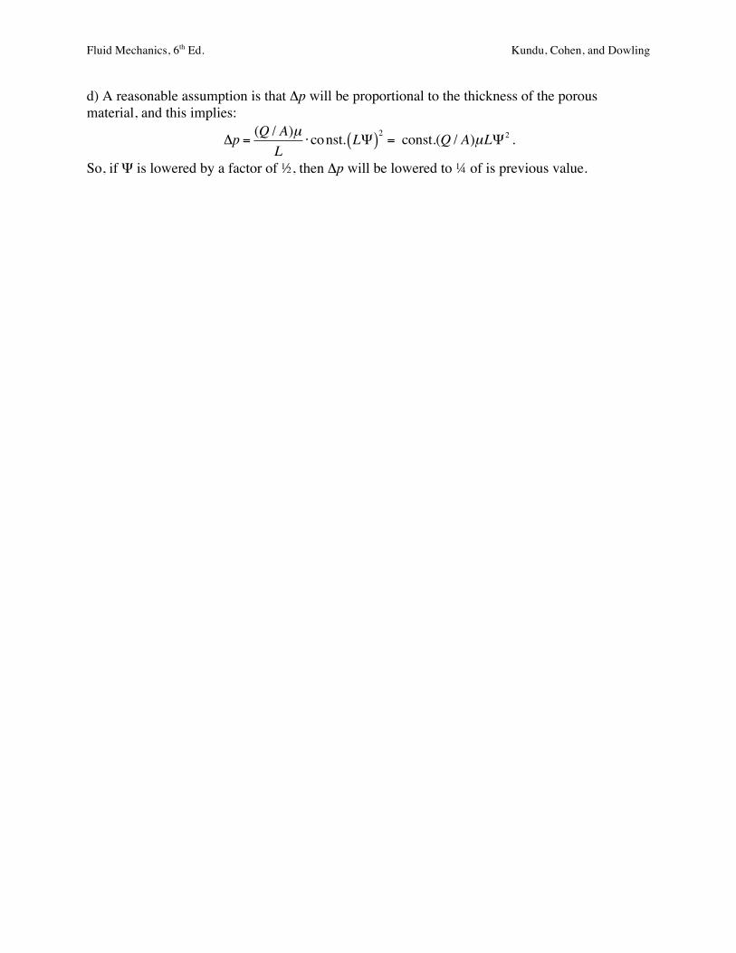
Fluid Mechanics, 6th Ed. Kundu, Cohen, and Dowling
d) A reasonable assumption is that Δp will be proportional to the thickness of the porous material, and this implies:
Δp = (Q / A)µL
⋅const. LΨ( )2= const.(Q / A)µLΨ2 .
So, if Ψ is lowered by a factor of ½, then Δp will be lowered to ¼ of is previous value.

Fluid Mechanics, 6th Ed. Kundu, Cohen, and Dowling
Exercise 1.47. A new industrial process requires a volume V of hot air with initial density ρ to be moved quickly from a spherical reaction chamber to a larger evacuated chamber using a single pipe of length L and interior diameter of d. The vacuum chamber is also spherical and has a volume of Vf. If the hot air cannot be transferred fast enough, the process fails. Thus, a prediction of the transfer time t is needed based on these parameters, the air’s ratio of specific heats γ, and initial values of the air’s speed of sound c and viscosity µ. a) Formulate a dimensionless scaling law for t, involving six dimensionless groups. b) Inexpensive small-scale tests of the air-transfer process are untaken before construction of the commercial-scale reaction facility. Can all these dimensionless groups be matched if the target size for the pipe diameter in the small-scale tests is d´ = d/10? Would lowering or raising the initial air temperature in the small-scale experiments help match the dimensionless numbers? Solution 1.47. a) This question can be answered with dimensional analysis. The parameters are drawn from the problem statement. The solution parameter is t, and the unit matrix is: t V Vf L d γ c ρ µ ––––––––––––––––––––––––––––––––––––––––––––––––– M 0 0 0 0 0 0 0 1 1 L 0 3 3 1 1 0 1 -3 -1 T 1 0 0 0 0 0 -1 0 -1 The rank of this matrix is 3, so there will be: 9 – 3 = 6 dimensionless groups. These groups are: a dimensionless time: Π1 = ct/d; a volume ratio: Π2 = V/Vf; another volume ratio: Π2 = d3/Vf; an aspect ratio: Π4 = L/d; the ratio of specific heats: Π5 = γ; and a sonic Reynolds number: Π6 = ρcd/µ. Thus, the scaling law is:
ctd= φ
VVf
, d3
Vf
, Ld,γ, ρcd
µ
!
"##
$
%&& .
b) The first dimensionless group will be matched if the other five are matched. So, let primes denote the small-scale test parameter. Matching the five independent dimensionless groups means:
VVf
=!V!Vf
, d3
Vf
=!d 3
!Vf
, Ld=
!L!d, γ = γ´, and ρcd
µ=
!ρ !c !d!µ
. (1, 2, 3, 4, 5)
Starting from the target pipe size ratio, d´ = d/10, (2) implies: d3
!d 3 =Vf
!Vf
=103 or !Vf =Vf 103 , and !V =V 103 .
where the finding for V´ follows from (1). Similarly, from (3), the results for the length of the pipe are:
d!d=L!L=10 , so !L = L 10 .
The next independent dimensionless group, γ, can be matched by using air in the scale model tests since it will be used in the full-scale device. The final independent dimensionless group is likely to be the most difficult to match. Using (5) and d´ = d/10, implies:

Fluid Mechanics, 6th Ed. Kundu, Cohen, and Dowling
ρcdµ
=!ρ !c d10 !µ
or !ρ !c!µ=10 ρc
µ,
and this relationship only involves material properties. The initial temperature (and pressure P) of the small scale experiments can be varied, ρ is proportional to T–1 (and P+1), while both c and µ are proportional to T1/2 (and nearly independent of P). Thus, small scale testing at reduced temperature (and elevated pressure) might make it possible to match values of this dimensionless group between the large- and small-scale experiments.

Fluid Mechanics, 6th Ed. Kundu, Cohen, and Dowling
Exercise 1.48. Create a small passive helicopter from ordinary photocopy-machine paper (as shown) and drop it from a height of 2 m or so. Note the helicopter’s rotation and decent rates once it’s rotating steadily. Repeat this simple experiment with different sizes of paper clips to change the helicopter’s weight, and observe changes in the rotation and decent rates. a) Using the helicopter’s weight W, blade length l, and blade width (chord) c, and the air’s density ρ and viscosity µ as independent parameters, formulate two independent dimensionless scaling laws for the helicopter’s rotation rate Ω, and decent rate dz/dt. b) Simplify both scaling laws for the situation where µ is no longer a parameter. c) Do the dimensionless scaling laws correctly predict the experimental trends? d) If a new paper helicopter is made with all dimensions smaller by a factor of two. Use the scaling laws found in part b) to predict changes in the rotation and decent rates. Make the new smaller paper helicopter and see if the predictions are correct.
Solution 1.48. The experiments clearly show that Ω and dz/dt increase with increasing W. a) This question can be answered with dimensional analysis. The parameters are drawn from the problem statement. The first solution parameter is Ω (the rotation rate) and the units matrix is: Ω W l c ρ µ –––––––––––––––––––––––––––––––– M 0 1 0 0 1 1 L 0 1 1 1 -3 -1 T -1 -2 0 0 0 -1 The rank of this matrix is 3, so there will be: 6 – 3 = 3 dimensionless groups. These groups are: Π1 = Ωρ1/2l2/W1/2, Π2 = l/c, and Π3 = ρW/µ2. Thus, the scaling law is:
Ωρl4
W= φ
lc, ρWµ 2
"
#$
%
&' ,
where φ is an undetermined function. The second solution parameter is dz/dt (the descent rate), and it has the same units as Ωl, so it's scaling law is:
dzdt!
"#
$
%&
ρl2
W=ψ
lc, ρWµ 2
!
"#
$
%& .
where ψ is an undetermined function.
4 cm!
7 cm!
2 cm!paper clip!
7 cm!

Fluid Mechanics, 6th Ed. Kundu, Cohen, and Dowling
b) When µ is no longer a parameter, both scaling laws simplify
Ωρl4
W=Φ
lc#
$%&
'( and dz
dt!
"#
$
%&
ρl2
W=Ψ
lc!
"#$
%& ,
where Φ and Ψ are different undetermined functions. These laws imply
Ω =1l2
WρΦ
lc#
$%&
'( and dz
dt=1l
WρΨ
lc"
#$%
&' ,
c) These scaling laws are consistent with experimental results; the rotation and decent rates both increase when W increases. d) If the aspect ratio, l/c, is fixed, then decreasing l by a factor of two should increase Ω by a factor of 4, and dz/dt by a factor of two. When the smaller helicopter is made, the experiments do appear to confirm these predictions; both Ω and dz/dt do increase, and the increase for Ω is larger.