modeling of the viscous e ects in uids - core.ac.uk · @y = 1 ˆ @p 0 @z + @2u @y2 ... ira m. cohen...

Modeling of the viscous effects in fluidscontained within a narrow pipe system

supplied by a jet

Peter Bergesen Kolstø

June 17, 2013

Contents

1 Introduction 11.1 Background . . . . . . . . . . . . . . . . . . . . . . . . . . . . 11.2 The aim of this thesis . . . . . . . . . . . . . . . . . . . . . . . 2

2 Cylindrical Laminar Jet 52.1 Background . . . . . . . . . . . . . . . . . . . . . . . . . . . . 52.2 Exact Solution . . . . . . . . . . . . . . . . . . . . . . . . . . 62.3 Analysis . . . . . . . . . . . . . . . . . . . . . . . . . . . . . . 10

2.3.1 The stream function . . . . . . . . . . . . . . . . . . . 102.3.2 The radial velocity . . . . . . . . . . . . . . . . . . . . 122.3.3 The axial velocity . . . . . . . . . . . . . . . . . . . . . 132.3.4 Momentum Flux . . . . . . . . . . . . . . . . . . . . . 14

2.4 Discussion . . . . . . . . . . . . . . . . . . . . . . . . . . . . . 152.4.1 The edge of the jet . . . . . . . . . . . . . . . . . . . . 162.4.2 The orifice from where the jet emerges . . . . . . . . . 162.4.3 Stability . . . . . . . . . . . . . . . . . . . . . . . . . . 172.4.4 The effects of fluctuations in the pressure gradient on

the jet . . . . . . . . . . . . . . . . . . . . . . . . . . . 172.4.5 The transition from jet to regular turbulent flow . . . . 18

3 Turbulent Flow Near a Wall 193.1 Background . . . . . . . . . . . . . . . . . . . . . . . . . . . . 193.2 The analysis made by von Karman . . . . . . . . . . . . . . . 193.3 Turbulent motion near a cylindrical wall . . . . . . . . . . . . 203.4 The thickness of the boundary layer . . . . . . . . . . . . . . . 213.5 Volume flow . . . . . . . . . . . . . . . . . . . . . . . . . . . . 223.6 Discussion . . . . . . . . . . . . . . . . . . . . . . . . . . . . . 23

4 Changing Pressure Gradient 25

5 Compressibility 27

3

4 CONTENTS

6 Oscillating Flow 296.1 Background . . . . . . . . . . . . . . . . . . . . . . . . . . . . 296.2 Mathematical considerations . . . . . . . . . . . . . . . . . . . 30

6.2.1 Transformation of the velocity profile . . . . . . . . . . 306.2.2 Closing the contour . . . . . . . . . . . . . . . . . . . . 326.2.3 Transform of pressure functions and distributions . . . 336.2.4 The poles of the function f(ω) . . . . . . . . . . . . . . 35

6.3 Calculation of responses . . . . . . . . . . . . . . . . . . . . . 366.3.1 Impulse response . . . . . . . . . . . . . . . . . . . . . 376.3.2 Frequency response . . . . . . . . . . . . . . . . . . . . 416.3.3 Step response . . . . . . . . . . . . . . . . . . . . . . . 43

7 Conclusion 47

8 References 49

List of Figures

1.1 General draft of the system under consideration. The streamlines

here predict what we intuitively would expect to happen to a jet

that is let into the pipe system shown. . . . . . . . . . . . . . . . 2

2.1 A simple sketch of a jet emerging from a small orifice into a large

pool of quiescent fluid. The thick lines starting at the orifice serves

to illustrate how we might perceive the edge of the jet. . . . . . . 62.2 Plot of the stream function for the cylindrical jet given in eq. 2.25.

It should be noted that we have disregarded the viscosity. . . . . . 112.3 Illustration of how we would expect the stream function of a cylin-

drical jet to behave. We note how the surrounding fluid is being

entrained onto the jet . . . . . . . . . . . . . . . . . . . . . . . . 122.4 A logarithmic plot of the radial velocity for a cylindrical jet. We

note the deviating behavior close to Z = 0. . . . . . . . . . . . . 132.5 The axial velocity of a cylindrical jet. Here plotted without the

scaling factor (ν/Z). . . . . . . . . . . . . . . . . . . . . . . . . 142.6 The momentum flux of a cylindrical jet, here plotted without the

scaling 128πρν2/Z2. . . . . . . . . . . . . . . . . . . . . . . . . 15

3.1 The velocity profile of a turbulent flow through a pipe for (blue

line). Plotted in contrast to the Possuille-Hagen profile (red line). . 21

6.1 The contour enclosing the poles in question. The dots placed sym-

metrically along the imaginary axis illustrates the first few poles of

the Bessel function in eq. 6.8. The lone dot on the positive imag-

inary axis near the origin, is situated at the location of the pole

of the transform of the step function and serves as an example of

how poles contributed by the transform of pressure functions are

included in the contour. . . . . . . . . . . . . . . . . . . . . . . 336.2 Impulse response of the pipe system . . . . . . . . . . . . . . . . 406.3 Frequency response of a straight pipe filled with fluid. . . . . . . 43

5

6 LIST OF FIGURES

6.4 Step response of the pipe system. . . . . . . . . . . . . . . . . . 45

Chapter 1

Introduction

1.1 Background

Industrial robots used to spray-paint vehicles use air to place the paint ontothe object. The paint is let out at the end of the robot arm, while a stream ofair is used to lead the paint towards its desired location. The air supplied tothe system comes from a control unit1 consisting of a high pressure chamberseparated from a pipe system by a valve. The valves position as a functionof time is preset according to the users desires. Adjustments are then madeaccording to measurements taken of the volume flow through the system. Wewill regard the ACU as a system consisting of two separate subsystems. Thetwo subsystems are the pipe system supplying the air to the robots tool andthe measuring arrangement used to obtain readings of the flow.

We will in this thesis analyze a design where the pipe system is supplied bya valve letting a circular laminar jet into it. The model given here is firstand foremost intended to be used to describe the pipe system, but to somelesser degree it also applies to the measuring arrangement. Modeling theinlet as a circular laminar jet is to be considered a suggestion of how to fillthe system with fluid. There might be different arrangements that could beused just as well. The reasons for me to chose this particular configuration isthat it is mathematically convenient and that it can be assumed to minimizesthe effects created as the fluid let in meets the inner walls of the pipe. Thestraight part of the pipe beyond the valve serves to stabilize the flow before

1The control unit in question is referred to as a ACU, which is short for air controlunit.

1

2 CHAPTER 1. INTRODUCTION

any measurement of it is obtained.

The measurements are done by utilizing a venturi. A venturi consists of twocylindrical pipes with a contracting part in between, which makes up thepipe system. The measurements are obtained by letting some air leak fromthe pipe system through much narrower pipes on either side of the contract-ing part of the pipe system to reach a pressure gauge at the end. Thesenarrow pipes makes up the measuring arrangement. The gauge operates byregistering the pressure associated with the volume flow through the narrowpipe. The difference between the pressure readings on either side are thenused to obtain a measurement of the volume flow through the pipe system.The general description of the system is illustrated in figure 1.12

Figure 1.1: General draft of the system under consideration. The streamlines

here predict what we intuitively would expect to happen to a jet that is let into

the pipe system shown.

1.2 The aim of this thesis

In order to analyze the behavior of the fluid moving through this system wewill divide the pipe into three separate sections. Each section will be an-alyzed in an individual chapter, considering stationary, incompressible flowonly. To take into account that the fluid moving through the real systemis not stationary, an additional chapter will consider the fluctuation in the

2The figure does not show the measuring arrangement as it is not considered a part ofthe pipe system, but a separate part of the system as a whole.

1.2. THE AIM OF THIS THESIS 3

pressure at the inlet. There will also be separate chapters discussing theeffects of compressibility and the effects of a changing pressure gradient inthe system.

The first section concerns how the fluid behaves as it emerges from a verysmall orifice into a large pool of quiescent fluid. The stream will here betreated as a laminar jet, described in cylindrical coordinates. Then as theboundary of the jet reaches the inner walls of the pipe, the second sectionwill aim to describe a turbulent stream contained within a straight, cylindri-cal pipe. We will include a chapter qualitatively discussing the effects of achanging pressure gradient as the pipe contracts, in order to give a completedescription of the pipe system. Then there will be a chapter considering theeffects of compressibility. We shall here use dimensional analysis to arguethe dominance of the viscous effects over the effects of compressibility. Thefluctuation will be analyzed using a known solution for how a harmonicallyoscillating pressure disturbance propagates through a flow in a pipe. Thissolution will be elaborated and expanded to include pressure disturbances inthe form of a step and an impulse distribution as well.

This thesis will combine elements from both applied physics and electro engi-neering in an attempt to describe a model of the pipe system and to analyzethe valve and the method used for measuring the stream. We will thereforenot present a pure mathematical model, but also include some qualitativeconsiderations and notation used in electro engineering. It is my intention tomake somewhat complicated mathematical considerations available and easyto apply to practical engineering.

4 CHAPTER 1. INTRODUCTION

Chapter 2

Cylindrical Laminar Jet

2.1 Background

The mathematical description of a narrow jet of high speed fluid emergingfrom a small orifice, i.e a laminar jet1, is derived by using the same as-sumptions as for a laminar boundary layer. The important facts under thisconsideration is that the pressure across the jet can not vary to a large extent,and thus, must be approximately the same as the pressure in the surround-ing fluid, and that the viscous forces in the direction of motion will be muchsmaller than those in the radial direction.

Disregarding gravity, as the jet is presumed to move horizontally, and flowin the azimuthal direction; the Navier-Stokes equation for a jet in Cartesiancoordinates is reduced to

u∂u

∂x+ v

∂u

∂y=

1

ρ

∂p0∂z

+ ν∂2u

∂y2. (2.1)

This equation in conjunction with the continuum equation

∂u

∂x+∂v

∂y= 0, (2.2)

describes the motion of a two-dimensional high speed jet in Cartesian coor-dinates. Here u and v represents the velocities and x, y and z the spacial

1The material in this subsection is found in [2] Pijush K. Kundu, Ira M. Cohen andDavid R. Dowling ’Fluid Mechanics’, unless otherwise stated

5

6 CHAPTER 2. CYLINDRICAL LAMINAR JET

coordinates. The density of the fluid is written ρ and the dynamical vis-cosity is written ν. The solution to this problem is well know and valid fora stationary, incompressible, two-dimensional, laminar, high speed jet, de-scribed in Cartesian coordinates that emerges from a narrow slit into a poolof quiescent fluid.

2.2 Exact Solution

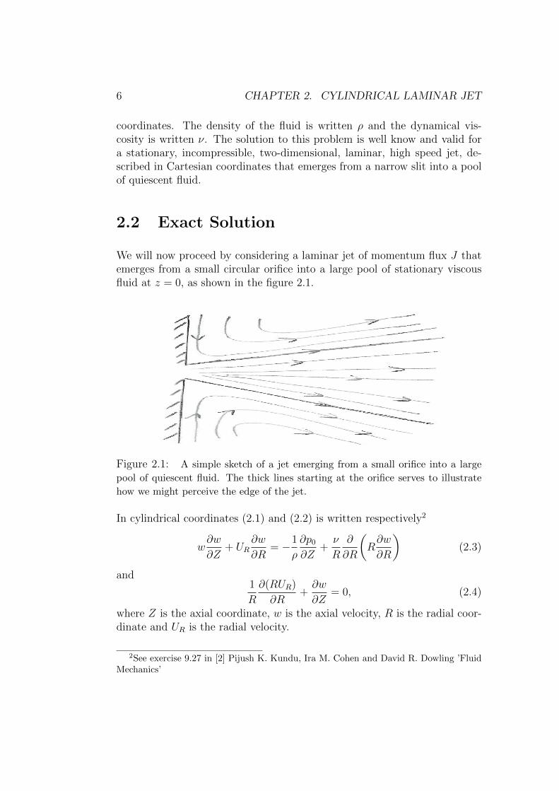
We will now proceed by considering a laminar jet of momentum flux J thatemerges from a small circular orifice into a large pool of stationary viscousfluid at z = 0, as shown in the figure 2.1.

Figure 2.1: A simple sketch of a jet emerging from a small orifice into a large

pool of quiescent fluid. The thick lines starting at the orifice serves to illustrate

how we might perceive the edge of the jet.

In cylindrical coordinates (2.1) and (2.2) is written respectively2

w∂w

∂Z+ UR

∂w

∂R= −1

ρ

∂p0∂Z

+ν

R

∂

∂R

(R∂w

∂R

)(2.3)

and1

R

∂(RUR)

∂R+∂w

∂Z= 0, (2.4)

where Z is the axial coordinate, w is the axial velocity, R is the radial coor-dinate and UR is the radial velocity.

2See exercise 9.27 in [2] Pijush K. Kundu, Ira M. Cohen and David R. Dowling ’FluidMechanics’

2.2. EXACT SOLUTION 7

Utilizing the continuum equation we seek a similarity solution3 for the streamfunction Ψ(η). We note that as we utilize the continuum equation we areassuming that there is no fluid entering or leaving the system. This is ofcourse unphysical as we here are considering a jet suppling fluid to largequiescent pool, but we do this in an attempt to simplify the model. Theerror resulting from this simplification will be analyzed in more detail at theend of this chapter.

Ψ = c1Rg(η), where η = (R/Z). (2.5)

The axial and radial velocity are found from the stream function as

w(η) ≡(

1

R

)∂Ψ

∂R= (c1/Z)

((1/η)g(η) + g′(η)

)(2.6)

and

UR(η) ≡ −( 1

R

)∂Ψ

∂Z= (c1/Z)ηg′(η). (2.7)

We now definef(η) ≡

((1/η)g(η) + g′(η)

), (2.8)

which gives us

ηf(η) =∂

∂η

(ηg(η)

)⇒ g(η) =

1

η

∫ η

ηf(η)dη (2.9)

and

g′(η) = −( 1

η2

)∫ η

ηf(η)dη + f(η). (2.10)

Substitution of (2.9) and (2.10) into (2.6) and (2.7) enables us to expressboth the axial and radial velocities as a function of f(η) respectively as

w(η) =(c1Z

)f(η) (2.11)

and

UR(η) =(c1Z

)(ηf(η)−

(1

η

) ∫ η

ηf(η)dη). (2.12)

It is clear from dimensional analysis that since η is a dimensionless variable,c1 must have the dimension L2/T in order for (2.11) and (2.12) to have

3We here refer to [1] D. J. Tritton ’Physical Fluid Dynamics’


dimension L/T . Thus, we expect that c1 must be the kinematic viscosity ofthe fluid. As such, we will further on use c1 = ν, which enables us to rewrite(2.11) and (2.12) respectively as

w(η) =( νZ

)f(η) (2.13)

and

UR(η) =( νZ

)(ηf(η)−

(1

η

) ∫ η

ηf(η)dη). (2.14)

The terms in (2.3) is found as

∂w

∂z= −

( νz2

) ∂∂η

(ηf(η)

),

∂w

∂R=( νz2

)f ′(η)

and∂

∂R

(R∂w

∂R

)=( νz2

) ∂∂η

(ηf ′(η)

).

As the fluid surrounding the jet is said to be quiescent we disregard thepressure gradient

∂p0∂z≈ 0.

Substituted into (2.3) the Navier-Stoke equation for a cylindrical jet reducesto

f ′(η) + ηf ′′(η) + ηf(η)2 + f ′(η)

∫ η

ηf(η)dη = 0. (2.15)

In order to solve this, we notice that

f ′(η) + ηf ′′(η) =∂

∂η

(ηf ′(η)

)and that

ηf(η)2 + f ′(η)

∫ η

ηf(η)dη =∂

∂ηf(η)

∫ η

ηf(η)dη.

This further reduces (2.15) to

ηf ′(η) + f(η)

∫ η

ηf(η)dη = 0. (2.16)

2.2. EXACT SOLUTION 9

In order to solve eq. (2.16) we introduce

F (η) ≡∫ η

ηf(η)dη. (2.17)

The first and second derivative of F (η) are respectively

F ′(η) = ηf(η) (2.18)

andF ′′(η) = f(η) + ηf ′(η). (2.19)

Substitution of eq. 2.17, eq. 2.18 and eq. 2.19 into (2.16) yields

ηF ′′(η) + F ′(η)(F (η)− 1

)= 0. (2.20)

Preceding to solve this we first notice that

F ′(η)(F (η)− 1

)=

1

2

∂

∂η

(F (η)− 1

)2and that

ηF ′′(η) =∂

∂η

(ηF ′(η)

)− F ′(η).

.

This produces

∂

∂η

(ηF ′(η)

)− F ′(η) +

1

2

∂

∂η

(F (η)− 1

)2= 0⇔

ηF ′(η)− F (η) +1

2

(F (η)− 1

)2= K1. (2.21)

We choose the value of K1 in such a manner that F (0) = 0. The value of K1

can then be determined as follows

K1 = ηF ′(η)− F (η) +1

2

(F (η)− 1

)2∣∣∣∣η=0

=1

2.

Now we can precede to solve (2.21) with K1 = 1/2

ηF ′(η)− F (η) +1

2

(F (η)− 1

)2=

1

2.


This yields

2η∂F

∂η= F (η)

(4− F (η)

).

Integrating this and utilizing that F (η)→ 0 for y → 0, we find

ln(η2) = ln

∣∣∣∣∣ F (η)

4− F (η)

∣∣∣∣∣+K2,

which yields

F (η) =4K2η

2

K2η2 + 1. (2.22)

By redefining g(η), found in eq. 2.5, we can chose that K2 = 1, thus we have

F (η) =4η2

η2 + 1. (2.23)

Differentiating this we find an expression for f(η)

f(η) =8

(η2 + 1)2. (2.24)

The solution found in eq. 2.24 determines the characteristics of the jet.Further on we will derive the stream function, the radial and axial velocityand the momentum flux of the jet from this function.

2.3 Analysis

2.3.1 The stream function

Substituting (2.24) into (2.9) and further substitution of this into (2.5) withc1 = ν, gives us the following expression for the stream function of the jetunder consideration as we substitute R/Z for η4:

Ψ(η) = νRg(η) = ν(Rη

)∫ η

ηf(η)dη

4We consider Ψ a function of η only for constant ν and R, and use the same consid-eration for other functions derived from the stream function during this chapter i.e. thefunctions for the axial and radial velocities and for the momentum flux.

2.3. ANALYSIS 11

= −ν(4R

η

)( 1

η2 + 1

)= −ν 4Z

R2/Z2 + 1= −ν 4Z3

R2 + Z2. (2.25)

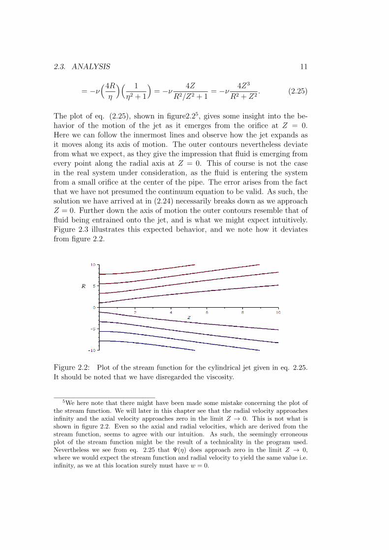
The plot of eq. (2.25), shown in figure2.25, gives some insight into the be-havior of the motion of the jet as it emerges from the orifice at Z = 0.Here we can follow the innermost lines and observe how the jet expands asit moves along its axis of motion. The outer contours nevertheless deviatefrom what we expect, as they give the impression that fluid is emerging fromevery point along the radial axis at Z = 0. This of course is not the casein the real system under consideration, as the fluid is entering the systemfrom a small orifice at the center of the pipe. The error arises from the factthat we have not presumed the continuum equation to be valid. As such, thesolution we have arrived at in (2.24) necessarily breaks down as we approachZ = 0. Further down the axis of motion the outer contours resemble that offluid being entrained onto the jet, and is what we might expect intuitively.Figure 2.3 illustrates this expected behavior, and we note how it deviatesfrom figure 2.2.

Figure 2.2: Plot of the stream function for the cylindrical jet given in eq. 2.25.

It should be noted that we have disregarded the viscosity.

5We here note that there might have been made some mistake concerning the plot ofthe stream function. We will later in this chapter see that the radial velocity approachesinfinity and the axial velocity approaches zero in the limit Z → 0. This is not what isshown in figure 2.2. Even so the axial and radial velocities, which are derived from thestream function, seems to agree with our intuition. As such, the seemingly erroneousplot of the stream function might be the result of a technicality in the program used.Nevertheless we see from eq. 2.25 that Ψ(η) does approach zero in the limit Z → 0,where we would expect the stream function and radial velocity to yield the same value i.e.infinity, as we at this location surely must have w = 0.


Figure 2.3: Illustration of how we would expect the stream function of a cylin-

drical jet to behave. We note how the surrounding fluid is being entrained onto

the jet .

2.3.2 The radial velocity

Substituting (2.24) into (2.14) yields and expression for the radial velocityas a function of η.

UR(η) =( νZ

)(ηf(η)−

(1

η

) ∫ η

ηf(η)dη)

= −( νZ

)4(η2 − 1)

(η2 + 1)2(2.26)

From eq (2.26) it is seen that

UR > 0 for η < 1,

UR = 0 for η = 1,

UR < 0 for η > 1. (2.27)

The result for η < 1 is in agreement with our intuition as we expect the radialvelocity to be positive, but decreasing as we move along the radial coordinateaway from the center of the jet. Then UR = 0 is reached as η = 1⇔ Z = R.For η > 1 we find the radial velocity to be directed towards the center ofthe jet. This might seem strange, but can be explained as the velocity of thesurrounding fluid being entrained onto the jet.

The error previously discussed, that arises from the fact that we are uti-lizing the continuum equation in a model of a jet results in a behavior ofthe radial velocity in the model that deviates from what we are expecting.This is shown in figure 2.4, which illustrates a strange behavior in the radial

2.3. ANALYSIS 13

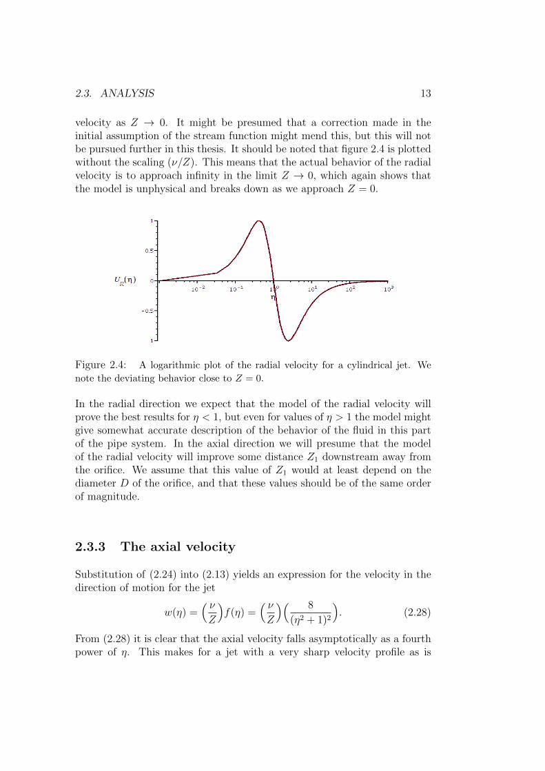
velocity as Z → 0. It might be presumed that a correction made in theinitial assumption of the stream function might mend this, but this will notbe pursued further in this thesis. It should be noted that figure 2.4 is plottedwithout the scaling (ν/Z). This means that the actual behavior of the radialvelocity is to approach infinity in the limit Z → 0, which again shows thatthe model is unphysical and breaks down as we approach Z = 0.

Figure 2.4: A logarithmic plot of the radial velocity for a cylindrical jet. We

note the deviating behavior close to Z = 0.

In the radial direction we expect that the model of the radial velocity willprove the best results for η < 1, but even for values of η > 1 the model mightgive somewhat accurate description of the behavior of the fluid in this partof the pipe system. In the axial direction we will presume that the modelof the radial velocity will improve some distance Z1 downstream away fromthe orifice. We assume that this value of Z1 would at least depend on thediameter D of the orifice, and that these values should be of the same orderof magnitude.

2.3.3 The axial velocity

Substitution of (2.24) into (2.13) yields an expression for the velocity in thedirection of motion for the jet

w(η) =( νZ

)f(η) =

( νZ

)( 8

(η2 + 1)2

). (2.28)

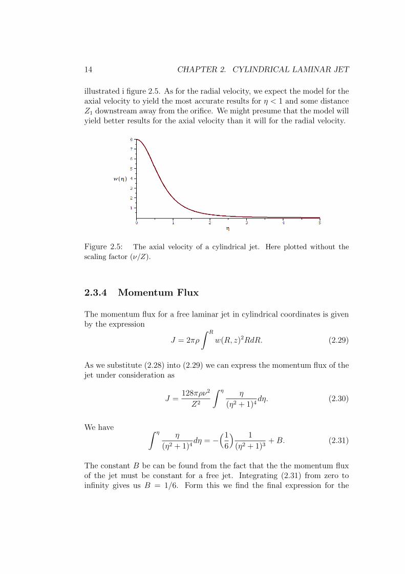
From (2.28) it is clear that the axial velocity falls asymptotically as a fourthpower of η. This makes for a jet with a very sharp velocity profile as is


illustrated i figure 2.5. As for the radial velocity, we expect the model for theaxial velocity to yield the most accurate results for η < 1 and some distanceZ1 downstream away from the orifice. We might presume that the model willyield better results for the axial velocity than it will for the radial velocity.

Figure 2.5: The axial velocity of a cylindrical jet. Here plotted without the

scaling factor (ν/Z).

2.3.4 Momentum Flux

The momentum flux for a free laminar jet in cylindrical coordinates is givenby the expression

J = 2πρ

∫ R

w(R, z)2RdR. (2.29)

As we substitute (2.28) into (2.29) we can express the momentum flux of thejet under consideration as

J =128πρν2

Z2

∫ η η

(η2 + 1)4dη. (2.30)

We have ∫ η η

(η2 + 1)4dη = −

(1

6

) 1

(η2 + 1)3+B. (2.31)

The constant B be can be found from the fact that the the momentum fluxof the jet must be constant for a free jet. Integrating (2.31) from zero toinfinity gives us B = 1/6. Form this we find the final expression for the

2.4. DISCUSSION 15

momentum flux to be:

J =128πρν2

Z2

(1

6− 1

6(η2 + 1)3

). (2.32)

Figure 2.6: The momentum flux of a cylindrical jet, here plotted without the

scaling 128πρν2/Z2.

It is seen from eq. (2.32) that the momentum flux falls as η to the sixthpower. This is shown in figure 2.6 where the momentum flux converges veryrapidly as η grows. As such, most of the momentum flux of the jet is con-tained within η < 1. This might be seen as support of the assumption thatthe model of the jet will generally prove the best results for η < 1.

We have not included any calculation of the volume flow for the laminar jet.The reason for this is that the bulk of fluid that makes up the jet increasesas more of the surrounding fluid is entrained onto the jet as it moves alongthe axis of motion. As such the momentum flux of the jet is the appropriateestimate for the size of the jet, as it remains the same for all values of Z.

2.4 Discussion

6

6We will in this subsection frequently refer to [1] D.J. Tritton ’Fluid Dynamics’


2.4.1 The edge of the jet

During operation the axial velocity is positive and non-zero inside the pipesystem for all values of R and Z. As such there will be a build up of a bound-ary layer along the entire pipe. Even so the axial velocity decreases rapidlyfor an increasing value of η, and as such it might be appropriate to define avalue which we can expect a build up of a significant boundary layer on theinside of the pipe system containing the jet. We have previously argued thatthe model of the jet will likely prove the best results for η < 1. From eq.(2.26) we have that the radial velocity reaches zero as η = 1. At this value ofη it can be seen from eq. (2.28), that the axial velocity have reduced to onefourth of its maximum. As such, we might use η = 1⇔ R = Z as a startingpoint for an experimental search for an appropriate value of η for which wecan define to be the edge of the jet.

We also have that the assumption of a free laminar jet necessarily must berendered invalid at some point because of the interference of the walls con-taining it. The error of this approximation will be omitted in this thesis, buthaving an edge of the jet enables us at least to measure the distance betweenthe wall of the pipe system and what we regard as the jet. By choosing R = Zas the edge of the jet we see that we have defined that jet will propagate in a45 degree angle in the radial direction as it moves along the axial direction.

2.4.2 The orifice from where the jet emerges

We will now discuss the consequences of utilizing the continuum equation ina model of a jet, and make clear the boundary conditions at the orifice fromwhere the jet emerges.

As we substitute η = R/Z into eq. (2.28) and eq. (2.26), we have in thelimit Z → 0 respectively

w(R,Z) = limZ→0

( νZ

)( 8

((R/Z)2 + 1)2

)= lim

Z→0

( 8νZ3

((R2 + Z2)2

)= 0 (2.33)

and

UR(R,Z) = limZ→0−(4ν

Z

) ((R/Z)2 − 1)

((R/Z)2 + 1)2= lim

Z→0−4νZ

(R2 − Z2)

(R2 + Z2)2= 0. (2.34)

2.4. DISCUSSION 17

From eq. (2.33) and eq. (2.34) we see that there is no fluid entering intothe system at Z = 0. The model therefore predicts that the jet is givenmomentum by a source emerging from an infinite small opening at (Z =0, R = 0) that is not providing any mass to the system. This is of courseunphysical, but it greatly simplifies the model. How the jet is given masscan be seen from dividing eq. (2.34) by eq. (2.33)

URw

=−(

4νZ

)(η2−1)(η2+1)2(

νZ

)8

(η2+1)2

= −1

2(η2 − 1) =

1

2(1− R2

Z2). (2.35)

Eq. (2.35) shows that as we approach Z = 0 the radial velocity grows towardsinfinity for all values of R. As such we find that the jet here is given its massfrom fluid being drawn from the surroundings onto the the center just beyondZ = 0.

2.4.3 Stability

The velocity profile of a jet as a turning point i.e. a non-zero value for itssecond derivative. We know from experimental data that flows of this kindare much more prone to instabilities than flows without. Hence, we pre-sume that the jet will most likely dissolve close to the point from where itemerges. Nevertheless the surrounding walls of the pipe will serve to stabilizethe jet, so that we might presume a jet structure of the flow for some lengthof the system. We will assume that the flow retains its characteristics as ajet at least long enough for its edge to reach the inner walls of the pipe i.e.η = 1⇔ R = Z.

2.4.4 The effects of fluctuations in the pressure gradi-ent on the jet

We presume that the effects that fluctuations of the pressure gradient in theflow will have upon both the jet and the surrounding fluid will be significant.An increase of the velocity of the flow will lead to a higher degree of stabilityin the jet, while a decrease will make it more unstable. What effects rapidfluctuations will have on the flow near the valve will not be pursued furtherin this thesis. Nevertheless we will presume that the fluctuations will cause


a larger degree of instabilities in the jet, and that this might cause it toundergo the inevitable transition from a structured laminar jet to a regularturbulent flow at a faster rate than a stationary jet.

2.4.5 The transition from jet to regular turbulent flow

We presume that as the jet breaks down because of the interference with thewall or because of instabilities within the jet itself the flow will undergo asudden transition from a laminar jet to a regular turbulent flow. We willpresume it to be crucial that this transition has taken place i.e. that the flowhas been stabilized enough for it to be described as a regular turbulent flow,before it reaches any point where measurements of it are obtained. It shouldbe noted that it would possible prove very hard to obtain proper readings ofthe flow as it undergoes the transition, and that this might also prove rightas we regard the jet as well.

Chapter 3

Turbulent Flow Near a Wall

3.1 Background

In this chapter we will presume the pipe to be filled with a more or lesshomogeneous turbulent flow. The high velocity of the flow required to makethe assumptions for the jet valid, results in a high Reynolds number in theflow following the jet. As such we can not hope to find an analytic solutionto the Navier-Stokes equation for the behavior of the flow. Instead we willrely on the analysis made by von Karman in his deduction of the behaviorof a turbulent shear flow near a wall in order to describe the stream in thispart of the system1.

3.2 The analysis made by von Karman

The boundary layer of a turbulent flow is divided into an inner laminarand an outer turbulent zone. As the velocity of the mean flow U can onlybe a function of the flow near the wall uτ , the kinematic viscosity ν and thedistance from the wall y, it is given from dimensional analysis that the profileof turbulent two-dimensional wall flows is

U

uτ=

1

K

[ln

(yuτν

)+ A

], (3.1)

1The material in this section here refer to [1] D.J. Tritton ’Fluid dynamics’, unlessotherwise stated

19

20 CHAPTER 3. TURBULENT FLOW NEAR A WALL

where K is the von Karman constant and A is an arbitrary constant of in-tegration. Experimentally the ratio U/uτ is found to be in the range 0.035to 0.05, and is found to depend rather weakly on the Reynolds number. Kis likewise experimentally found to be approximately equal to 0.40.

The logarithmic velocity profile for the turbulent part of a boundary layer,described in (3.1), proves the best results when 30 < yuτ/µ < 200, whereyuτ/µ scales the thickness of the turbulent boundary layer. Below this weexpect a linear velocity profile for the laminar part of the boundary layer.Above the boundary layer the profile will depend on the flow as a whole.From this we will presume that for any velocity high enough to produce aturbulent flow, we will have a very thin turbulent boundary layer and aneven thinner laminar layer underneath. The profile of the flow as a wholeand the profile of the laminar sublayer will deviate from the profile describedin this section. Nevertheless we shall presume that this logarithmic profilewill be a valid approximation in these region, but that it will agree the mostwith experimental results in the range given above.

3.3 Turbulent motion near a cylindrical wall

To be able to apply (3.1) to a flow through a cylindrical pipe we will makethe following assumption that y ≈ a− r2. We can do this as we already haveassumed that the thickness of the boundary layer is very small. Substitutionof this assumption into (3.1) gives the equation

U(r) =uτK

[ln

(a− ra

)+ ln

(auτν

)+ A

]. (3.2)

In the center of the pipe we find the maximum velocity of the flow throughthis part of the system to be

Um = U(0) =uτK

[ln

(auτν

)+ A

]. (3.3)

Using eq. 3.3 we can now rewrite eq. 3.2 as

U(r) = Um +uτK

[ln

(1− r

a

)], (3.4)

2We here refer to verbal information given by Per Amund Amundsen’

3.4. THE THICKNESS OF THE BOUNDARY LAYER 21

which gives us the velocity profile of a turbulent flow through a pipe. Fur-thermore we can use the experimental data given above to rewrite eq. 3.4as

U(r) = Um

(1 +

1

10

(ln(1− b)

)), (3.5)

where we have presumed the ratio utau/Um to be 0.04 and K to be 0.4. Wehave also introduced b as the ratio between the radial coordinate r and themaximum radius of the pipe a for the sake of convenience. From (3.5) it isclear that the shape of the velocity profile is given by the ratio b = r/a, andthat Um merely serves to scale this profile.

3.4 The thickness of the boundary layer

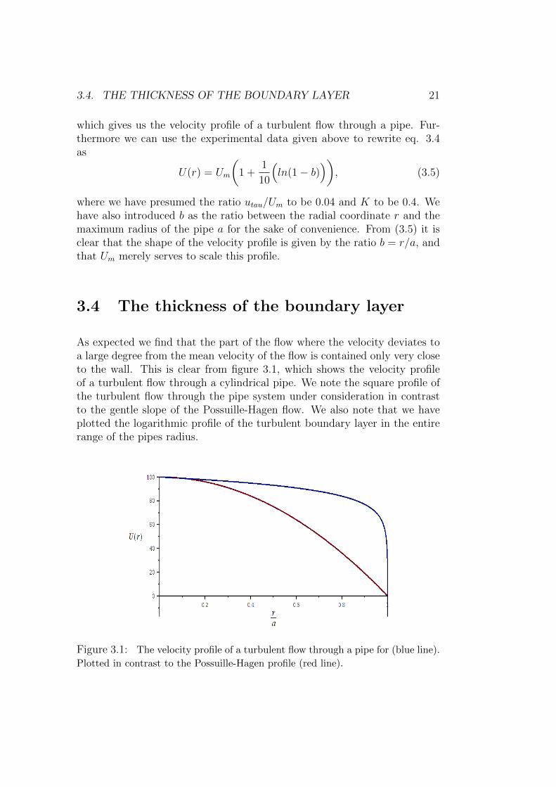
As expected we find that the part of the flow where the velocity deviates toa large degree from the mean velocity of the flow is contained only very closeto the wall. This is clear from figure 3.1, which shows the velocity profileof a turbulent flow through a cylindrical pipe. We note the square profile ofthe turbulent flow through the pipe system under consideration in contrastto the gentle slope of the Possuille-Hagen flow. We also note that we haveplotted the logarithmic profile of the turbulent boundary layer in the entirerange of the pipes radius.

Figure 3.1: The velocity profile of a turbulent flow through a pipe for (blue line).

Plotted in contrast to the Possuille-Hagen profile (red line).


A convenient way of measuring the thickness of the boundary layer wouldbe to define it to be at the value of r where the derivative of U(r) is equalto one. Another way would be to define it to be where the velocity is lessthan 99% of the mean velocity. With the first definition we find it to beb = 0.9999498, and with the second we find it to be b = 0.9999546, bothfor Um = 100 m/s. In either case we have such a thin boundary layer thatit can be neglected for any velocity of practical interest in the real system.Hence, we can conclude that we may disregard the velocity profile given inthis chapter and only consider the mean velocity as we describe the flow inthis section of the pipe system. We note that even as we might discard thethickness of the boundary layer we must still take into account how the non-slip condition affects the velocity profile in the pipe. We can therefore notutilize the maximum velocity in calculations of the volume flow, but mustinstead use the mean average velocity. The reason for this can be seen fromfigure 3.1, where we note how the velocity increases for a decreasing radialcoordinate outside the boundary layer as well as within. The boundary layeralso sustain the turbulence in the pipe system by transporting vorticity intothe main stream, and then there are the effects of separation and friction.

3.5 Volume flow

Even as the flow in this section of the pipe system can be pretty accuratelydescribed by its mean velocity we note that there will exist fluctuations ofthe velocity atop the mean velocity in a turbulent flow. These fluctuationsmight be significant considering the very turbulent nature of the flow in thereal system.

The solution for the volume flow as we apply eq. 3.5 along the entire radiusof the pipe is given as

Q = 2π

∫ a

0

u(r)rdr = 2πUm

∫ a

0

r

(1 +

1

10

[ln(

1− r

a

)])dr

,

= 2πUm

(∫ a

0

rdr +1

10

∫ a

0

r[ln(

1− r

a

)]dr

)= 2πUm

(1

2a2 − 3

40a2

)= 2πa2Um(0.425) = 0.85πa2Um (3.6)

3.6. DISCUSSION 23

From eq. (3.6) we see that even as the boundary layer is very thin the volumeflow is reduced to 42.5% of what the flow would have been if the maximumvelocity would have been present all over the radial axis.

3.6 Discussion

The assumption that y ≈ a − r made in the calculation of (3.4) leads to aresult that deviates some from what we expect from a physical point of view.We would expect that the derivative of the radial velocity with respect tothe radial coordinate should be zero at the center of the pipe. But as can beseen the derivative of (3.4) at r = 0 yields

dU(r)

dr

∣∣∣∣r=0

=uτaK6= 0. (3.7)

This results in a small deviation from what we would expect in the velocityprofile around the center of the pipe. The error here will in most cases beacceptable as the model yields a velocity that is accurate in the mean. Assuch, we keep eq. (3.6) as an appropriate approximation of the volume flow.

Chapter 4

Changing Pressure Gradient

To be able to give a complete description of the pipe system we will nowturn our attention to the contracting part of it and qualitatively consider theeffects the gradually decreasing diameter of the pipe system will have on theflow described in the previous chapter. This is not to be considered a partof the mathematical model of the system, but serves to clarify some aspectsassociated with the change of conditions in a boundary layer. We do this inan attempt to wheel this thesis in the direction of practical engineering andfurther design of the system.

In the case of a stationary flow we will have a favorable pressure gradient atthe contracting part of the pipe i.e.

∂u0∂x

> 0 ⇔ ∂p0∂x

< 0.

First and foremost, a smaller diameter will serve to increase the velocity anddecrease the pressure and thus stabilize the flow1. As the pressure decreasesthrough the contracting part of the pipe the turbulent boundary layer willbecome increasingly thinner. At the same time the increase of the Reynoldsnumber will cause the turbulence within the boundary layer to increase.Thus, the portion of the flow producing the turbulence will become smallereven as it produces more turbulence. This turbulence will be transportedinto the main stream.

The high velocity of the flow under normal operating procedures makes itunlikely that the boundary layer will separate under stationary conditions.

1We will in this chapter refer to [1] D. J. Tritton ’Physical Fluid Dynamics’

25

26 CHAPTER 4. CHANGING PRESSURE GRADIENT

Even so, we suspect that it will be more likely that the boundary layer willseparate at the points where the pipe system starts to and ceases to contract.We will expect that the increase of the instability in the boundary layer atthese locations will rely on the smoothness of the transition. If these transi-tions are not sufficiently smooth there might be areas contained close to thetransitions where we might have an adverse pressure gradient, which in turnmight cause a separation.

The effects caused by fluctuations will contribute to the conditions for sepa-ration of the boundary layer in the pipe system. As the velocity of the flowdecreases an adverse pressure gradient is produced in the entire flow. If thedecrease of the flow rate lasts long enough for the boundary layer to separate,there would be a significant increase in the transport of turbulence from theboundary layer into the main flow. As a consequence of this increased tur-bulence the mean velocity in the axial direction will slow down, as energy isneeded to maintain the higher degree of random motion of the fluid particles.

Chapter 5

Compressibility

The valve that separates the high pressure chamber and the pipe system isable to take on any range of openings, from complete shutdown, to lettingin air moving at sonic speed. We will presumed that the conditions for su-personic velocities are not present in the system1. Therefore the maximalvelocity of the stream i.e. the local speed of sound, is reached before thevalve has fully opened. Depending on the design of the valve the streammight nevertheless reach supersonic velocities as it is let into the pipe sys-tem, but we will then presume that the stream will return to sonic conditionsthrough the means of oblique shock waves short after. Typically the velocityof air through the system will range from 40 to 90m/s at the widest partand from 150 to 300m/s at the narrowest part of the pipe system. From thiswe have that the flow will reach velocities in the pipe system for which theeffect of compressibility will range from noticeable to very significant.

Compressibility becomes a significant effect as the fluid in question reachesvelocities of about 30% of the local speed of sound. For velocities below thisthe results reached by assuming incompressibility deviates from experimentalresults by less than 20%. The assumption of incompressibility will thereforeresult in an noticeable error in the real system under consideration, as thefluid used here is air of velocities approaching the local speed of sound. Evenso it will be made clear that the time constant of the effects caused by thecompressibility of the fluid is much smaller than the time constant of the ef-fects caused by the viscous forces. As such we can reasonably argue a modelof the system based on the viscous effects only. There will be effects caused

1We will in this chapter refer to [2] Pijush K. Kundu, Ira M. Cohen and David R.Dowling ’Fluid Mechanics’

27

28 CHAPTER 5. COMPRESSIBILITY

by compressibility, such as the shock waves created if the flow should passthe local speed of sound and the chocking of fluids moving at sonic velocities,that are not affected by this difference of the time constants, but they willnot be pursued further in this thesis.

Using dimensional analysis on the effects caused by compressibility in thepipe system under consideration, we have that the length scale is the dis-tance from the valve to the inlet of the pressure gauge and the velocity scaleis the speed of sound. If the medium is air, with a local speed of soundc ≈ 300m/s and a length from the inlet to the point of measuring l ≈ 10cm,we have that the time constant for the compressible effects is of the orderl/c ≈ 3 ∗ 10−4sek. We shall see in chapter 6 that the time scale for theviscous effects are of the order a2/ν. Using ν ≈ 1.5 ∗ 10−5m2/s for air underconditions associated with normal operating procedures, and a ≈ 1cm beinga typical radius for a pipe, the time scale of the viscous effects becomes of theorder a2/ν ≈ 6sek. We see that the time scale for the viscous effects will beabout 104 times larger than what the time scale for the compressible effectsare in this case. We presume that the effects of compressibility can be con-sidered linear with regard to the viscous effects. Hence, as we are concernedwith the time it takes for the volume flow to adjusts to changes in the pres-sure of the flow it seems appropriate to neglect the effects of compressibilityas we regard how the volume flow adjusts to changes of the pressure in theflow.

Chapter 6

Oscillating Flow

6.1 Background

The problems discussed so far apply to stationary flows only. As the realsystem under consideration operates with a unsteady flow we will now givesome consideration of how to mend this. Provided by Per Amund Amundsenis a solution for how a harmonically oscillating pressure affects the volumeflow through a pipe system. This chapter will elaborate and expand thatsolution to include other types of pressure changes in the flow. This expansionwill not be applied to the solution for the laminar jet as it is beyond the scopeof this thesis, but it will serve to give a model for how the stream behaves asit is considered to fill an entire straight pipe. As such the solution does notapply to the converging part of the pipe system. We note that the solutionsdiscussed here apply to an laminar flow in a straight pipe, and that thefluid through the real system is both turbulent and contracting. Even so,the solution given in this chapter will give a general overview of the processthat illustrates the mechanism of some of the determining variables. Thesevariables would among others be the time constant and the amplification ofthe process in the pipe system under consideration.

The solutions here will also serve to give a method of improved measure-ments of the flow as well as describing it. If the measurements of the floware done by attaching a separate pipe to the pipe system, as is the case weare considering here, then this model will apply to that pipe as well. Evenso we note that this model is developed in order to describe oscillating fluidmoving through pipes with a diameter a of some magnitude, and that somecaution might be called for as it is applied to a very narrow pipe.

29

30 CHAPTER 6. OSCILLATING FLOW

6.2 Mathematical considerations

6.2.1 Transformation of the velocity profile

The Navier-Stokes equation in cylindrical coordinates for a time-varying,incompressible, laminar flow in a straight pipe, with no flow in the azimuthaldirection and with the gravitational forces disregarded is reduced to

ρ∂u

∂t= −∂p

∂z+ µ

(∂2u

∂r2+

1

r

∂u

∂r

), (6.1)

with the pressure in the pipe system given by1

p(r, z, t) = p(z, t) = −∆p(t)

lz + p0(t). (6.2)

Eq. (6.1) can be solved by the use of Fourier analysis. In order to do so wewill transform every term in eq. (6.1) into the frequency domain and thentransform the entire equation back to the time domain.

We will here respectively use the following definition for the Fourier and theinverse Fourier transform2.

X(ω) =

∫ ∞−∞

x(t)e−iωt

x(t) =1

2π

∫ ∞−∞

X(ω)eiωt. (6.3)

From the definition given in (6.3) we have that eq. (6.1) equals

1

2π

∫ ∞−∞

[− ρ∂u

∂t− ∂p

∂z+ µ

(∂2u

∂r2+

1

r

∂u

∂r

)]eiωtdω = 0, (6.4)

1With reference to ’Per Amund Amundsens, unpublished note concerning oscillatingflows’

2We here refer to [3] B. P. Lathi ’Linear Systems and Signals’.

6.2. MATHEMATICAL CONSIDERATIONS 31

where u(r, w) and p(w) are the Fourier transform of u(r, t) and p(t) respec-tively.

The following theorem states that for any function F (x, y)3∫ ∞−∞

F (x, y)eiωtdω = 0 ∀ ω then F (x, y) = 0. (6.5)

Now, with reference to theorem (6.5) we see that eq. (6.4) is solved as longas

−ρ∂u∂t− ∂p

∂z+ µ

(∂2u

∂r2+

1

r

∂u

∂r

)= 0. (6.6)

Having transformed eq. (6.1) with regard to t only we find the terms in (6.6)to yield

∂u(ω, r)

∂t= iωu(r, ω)

and∂p(ω)

∂z= −∆p(ω)

µl,

while the last two terms remain unchanged with respect to there derivatives.Substitution of the transformed terms into eq. (6.6) enables us to rewrite itas

∂2u

∂r2+

1

r

∂u

∂r− iωρ

µu+

˜∆p(ω)

µl= 0. (6.7)

Subject to the boundary conditions u(a) = 0 and u(0) being finite. Thesolution of eq. (6.7) is given by

u(r, ω) =−i∆p(ω)

ρωl

(1−

J0(r√−iων

)J0(a√−iων

)), (6.8)

where J0 is a Bessel function of order zero.

The inverse Fourier transform of (6.8) yield the velocity profile in the timedomain

u(r, t) =1

2π

∫ ∞−∞

u(r, ω)eiωtdω. (6.9)

3We here refer to [4] George Arfken ’Mathematical Methods for Physicists’


It would be convenient to consider the poles contributed by the transformof the function for the pressure separate from the rest of the function in eq.(6.8). As such we define

f(ω) =1

ω

(1−

J0(r√−iων

)J0(a√−iων

))eiωt. (6.10)

We will now use eq. 6.10 to rewrite eq. 6.9

u(r, t) =−i

2πρl

∫ ∞−∞

∆p(ω)f(ω)dω. (6.11)

Eq. (6.11) is a complex function with poles. As such we will solve it by theuse of the theorem of residues4.

u(r, t) = 2πi∑k

Res

[−i

2πρl∆p(ω)f(ω), ω0

]=

1

ρl

∑k

Res

[∆p(ω)f(ω), ω0

],

(6.12)where ω0 are the poles of the functions in question.

The velocity profile can be determined from the sum of the residues con-tributed by the poles of the function f(ω) and ∆p(ω).

u(r, t) =1

ρl

(∑k

Res[ ˜∆p(ω)f(ω), ωk

]+∑m

Res[ ˜∆p(ω)f(ω), ωm

]), (6.13)

where ωk and ωm are the frequencies that yield poles in the function f(ω)

and the transform of the pressure function ˜∆p(ω) respectively.

6.2.2 Closing the contour

We will now proceed to close the contour around the residue in eq. 6.13.The important point then is to ensure that the part of the circle-integral notalong the real axis in eq. (6.9) does not contribute to the final value. As weare considering a real system we will only include positive values of the timet. From eq. (6.9) we see that the factor that might approach infinity for an

4We here refer to George Arfken ’Mathematical Methods for Physicists’


increasing value of t is eiωt, with ω = x + yi, we have eixte−yt, the absolutevalue of which is |e−yt|. It is imperative that |e−yt| → 0 on the part of thecircle-integral not along the real axis, from this it is seen that the contourmust be taken around the upper half plane. The contour will be encircled ina counterclockwise direction as the integral is taken from −∞ to ∞ along thereal axis. To ensure that the integral remains finite we shall therefore onlyinclude the poles contributed by the Bessel function and the transform ofthe pressure functions in the upper half plane. Figure 6.1 serves to illustratethis.

Figure 6.1: The contour enclosing the poles in question. The dots placed sym-

metrically along the imaginary axis illustrates the first few poles of the Bessel

function in eq. 6.8. The lone dot on the positive imaginary axis near the origin, is

situated at the location of the pole of the transform of the step function and serves

as an example of how poles contributed by the transform of pressure functions are

included in the contour.

6.2.3 Transform of pressure functions and distributions

We now turn our attention to the transforms of the pressure distributionsand functions5 in question from the time domain into the frequency domainand locate there poles. We will in this thesis only consider an impulse and astep distribution and a harmonic function6.

5Further on we will refer to both the functions and distributions of the pressure ingeneral we will simply call them functions.

6We will in this subsection refer to [3] B. P. Lathi ’Linear Systems and Signals’, unlessotherwise stated


Even though an impulse and a step distribution are not functions in theclassical sense, we have that they can still be transformed into and out ofthe frequency domain according to Fourier theorem as they here act uponanother function. As such they can still be subject to Fourier transform allthough they do not satisfy the Dirchlet conditions by themselves7.

Transform of a harmonic function

We will here represent a harmonic function for the pressure in the timedomain ∆p cos(ω0t) as the real part of a complex exponential ∆p<

[eiω0t

].8

The transform into the frequency domain is then given as

∆p(t) = ∆peiω0t ⇔ ∆p(ω) = ∆p

∫ ∞−∞

eiω0te−iωtdt

= ∆p

∫ ∞−∞

ei(ω−ω0)tdt = ∆pδ(ω − ω0) =∆p

πlimε→0

ε

(ω − ω0)2 + ε29. (6.14)

Here we have poles located in both ω = ω0 − iε and ω = ω0 + iε. Since thecontour excludes the lower half plane we will only have contributions fromω = ω0 + iε.

Transform of the impulse distribution

For an impulse distribution in the time domain ∆pδ(t) we have from thesampling theorem that the transform into the frequency domain is given as

∆p(t) = ∆pδ(t)⇔

∆p(ω) =

∫ ∞−∞

∆pδ(t)e−iωtdt = ∆p. (6.15)

It is clear from eq (6.15) that the transform of an impulse function doesnot contribute any poles in eq (6.13). It can be noted that to represent animpulse distribution in the time domain an equal amount of every possiblefrequency is needed in the frequency domain.

7We here refer to [5] Eugen Butkov ’Mathematical Physics’8Note that we further on will skip the notation < for the real part for the sake of

convenience. As such we must simply keep in mind that we are always considering realsystems and signals during all of this thesis.

9We here refer to [7] Frank W. Olver, Danile W. Lozier, Ronald F. Boisvert and CharlesW. Clark ’Nist handbook of mathematical functions’


Transform of the step distribution

A step distribution in the time domain ∆pθ(t) is represented in the frequencydomain as

∆p(t) = ∆pθ(t)⇔

∆p(ω) = ∆p

∫ ∞0

e−iωtdt =∆p

−iωe−iωt

∣∣∣∣∞0

=∆p

iω. (6.16)

In the form of a step distribution we have that the transform of the pressureyields a pole situated at ω = iε, where ε is an arbitrary small number. Itmight not be entirely clear from eq. 6.48 that the pole should be situatedhere, but as we consider the inverse transform it is clear that it must be thisway. This pole contributes to eq. (6.13)10.

6.2.4 The poles of the function f(ω)

We will now consider the poles from function f(ω) described in eq. 6.10 thatcontributes to the residue described of eq. 6.13 . The Bessel function in theenumerator in eq. 6.10 clearly contributes an infinite number of poles. Inaddition to this we must also consider whether there is a pole at ω = 0. Tosee that this is not the case we shall use the Taylor expansion of the Besselfunction around ω = 0 considering the two first terms only,

J0(zi) = J0(zi) + J ′0(zi)(z − zi) + J ′′0 (zi)(z − zi)2 + . . .⇒

J0(r

√−iων

)≈ 1−

(r√−iων

)24

= 1 +ir2ων

4. (6.17)

Having done the same expansion for the enumerator as for the numerator,we substitution eq. (6.17) into eq. (6.10) and find

f(0) = limω→0

1

ω

(1−

J0(r√−iων

)J0(a√−iων

))eiωt ≈ lim

w→0

1

ω

(1−(

1 + 14ir2ων

1 + 14ia2ων

))eiωt (6.18)

10In the following it shall always be assumed that iω is shorthand for ω − iε


As −1 < ω < 1 we can develop a series expansion of the enumerator throughthe relation

1

1 + x= 1− x+ x2 − x3 + x4 − . . . . (6.19)

Approximating eq. 6.18 by its two first terms, we have

f(0) ≈ limω→0

1

ω

(1−

(1 +

1

4

ir2ω

ν

)(1− 1

4

ia2ω

ν

))eiωt

= limω→0

1

ω

(1

4

ir2ω

ν− 1

4

ia2ω

ν+

1

16

a2r2ω2

ν2

)eiωt (6.20)

As we here are considering only very small values of ω, we will no discardthe second order term for w, in eq. 6.20. As such we have that

f(0) ≈ 1

ω

(i(a2 − r2) ω

4ν

)=i(a2 − r2)

4ν(6.21)

From (6.21) we see that not only do a zero in the last factor cancel the polein the first factor for very low frequencies, but we also regain the Poiseuille-Hagen velocity profile for the flow. This is in accordance with our expecta-tions from a physical point of view. It is now clear that the poles contributingto the residues of eq (6.13) comes only from the Bessel function and from thetransform of the pressure functions.

The poles contributed by the Bessel function in eq. (6.8) are

J0,k = (a

√−iωkν

)⇔ ωk = iν(J0,ka

)2, (6.22)

where J0,k refers to the real-valued zeros of a Bessel function of the orderzero. As J0(z) = J0(−z), we find that the poles contributed by the Besselfunction in eq. 6.8 are situated along the entire imaginary axis.

6.3 Calculation of responses

Having considered the general approach towards solving the problem of os-cillating flow, and as we have found the poles contributing to the residues,

6.3. CALCULATION OF RESPONSES 37

we will proceed to determine the velocity profiles that occur as a result of thedifferent pressure disturbances exiting the pipe system through the means ofviscous effects. From the velocity profiles we find the volume flow throughintegration. This enables us to express the response of the system as weregard the pressure at the inlet as the input signal and the correspondingvolume flow through the pipe system as the output.

Q(t) = 2π

∫ a

0

ru(r, t)dr = πa2u(t), (6.23)

where Q(t) denotes the corresponding volume flow and u(t) denotes the meanvelocity through the pipe.

6.3.1 Impulse response

Velocity profile response

The transform of an impulse distribution does not contribute any poles, andas such the only poles contributed to the residue in this case comes from thezeros of the Bessel function. They are of the first order, and as such theycan be calculated as follows

u(r, t) =1

ρl

∑k

Res[f(ω)∆p, ωk

]=

1

ρl

∑k

limω→ωk

∆pf(ω)(ω − ωk), (6.24)

where ωk = iν(j0,k/a)2.

We will now rewrite the function f(ω), found in eq. 6.10, as a fraction whereonly the factor contributing poles are written in the enumerator

f(ω) =h(ω)

g(ω)=

1ω

(J0(a√−iων

)− J0

(r√−iων

))eiωt

J0(a√−iων

) . (6.25)

Utilizing this we now write eq. 6.24 as

u(r, t) =1

ρl

∑k

limω→ωk

∆ph(ω)g(ω)

(ω−ωk)

=∆p

ρl

∑k

h(ω)

g′(ω)

∣∣∣∣∣ω=ωk

(6.26)


=∑k

∆p

ρl

((J0(a√−iων

)− J0

(r√−iων

))eiωt

−ωJ1(a√−iων

)√−ia24νω

)∣∣∣∣∣ω=

iνj20,k

a2

=2∆p

ρl

∑k

1

jo,k

(J0(rajo,k)

J1(jo,k) )e−ν( j0,ka )2t = G(r, t). (6.27)

Realizing the importance of eq. 6.27, as it represents the impulse responseof the system, we will define it as G(r, t). We note that the unit of G(r, t) is[m/s2] as it is required to be integrated over dt along with an other function.This corresponds to G(r, t) being a Greens function 11, which is a solution to

L{G(r, t− t′)} = δ(t− t′), (6.28)

where

L{} =∂2

∂r2+

1

r

∂

∂r+ρ

µ

∂

∂t. (6.29)

We then have that the velocity profile resulting from any pressure disturbancecan be found from

L{u(r, t)} = ∆p(t) (6.30)

With a solution that can be written as:

u(r, t) = u0(r, t) +

∫ −∞∞

G(r, t− t′)∆p(t′)dt′, (6.31)

which is a solution of the inhomogeneous problem with the stated boundaryconditions.

Volume flow response

We will now integrate of the velocity profile of the flow resulting from adisturbance of the pressure at the inlet in form of an impulse. From thiswe find the impulse response of the system. We note that the response isgiven with regard to how the volume flow inside the pipe system changes inresponse to changes of the pressure gradient.

Q(t) = 2π

∫ a

0

rG(r, t)dr

11We here refer to [4] George Arfken ’Mathematical Methods for Physicists’


=4π∆p

ρl

∑k

1

jo,ke−

j0,ka

2νt

∫ a

0

r

(J0(rajo,k)

J1(jo,k) )dr.

=4π∆pa2

ρl

∑k

1

j2o,ke−

j0,ka

2νt. (6.32)

We see that the first term of eq. 6.32 will dominate as it has the largestcoefficient and the largest time constant. As such we will here use

∑k j0,k ≈

2.5.

Q(t) ≈ ∆p(t)2a2

ρle−

6νa2t. (6.33)

In the Laplace domain this transforms to12

Hp(s) =Q(s)

∆p(s)≈ 2a2

ρl

1

s+ ν 6a2

=a4/3µl

(a2/6ν)s+ 1, (6.34)

where Hp(s) denotes the volume impulse response of the system in responseto pressure changes at the inlet. The amplification of the system is a4/3µland the time constant is a2/6ν. We see that they both increase with an in-creasing diameter of the pipe, and that they both decrease with an increaseof viscosity.

From the above we have that the model would predict that we could achievean arbitrary fast response by decreasing the diameter of the pipe. Here wenote that we have not considered the capillary effects. These effects arenormally small, but come into play when we are considering fluid movingthrough very narrow passages. Qualitatively we predict that the capillaryand viscous effects can be considered linear, and that the time constant ofthe capillary effects will increase rapidly as the radius of the pipe becomesvery small. Hence, we will reach a point where a decreasing diameter of thepipe will result in a increasing time constant of the system.

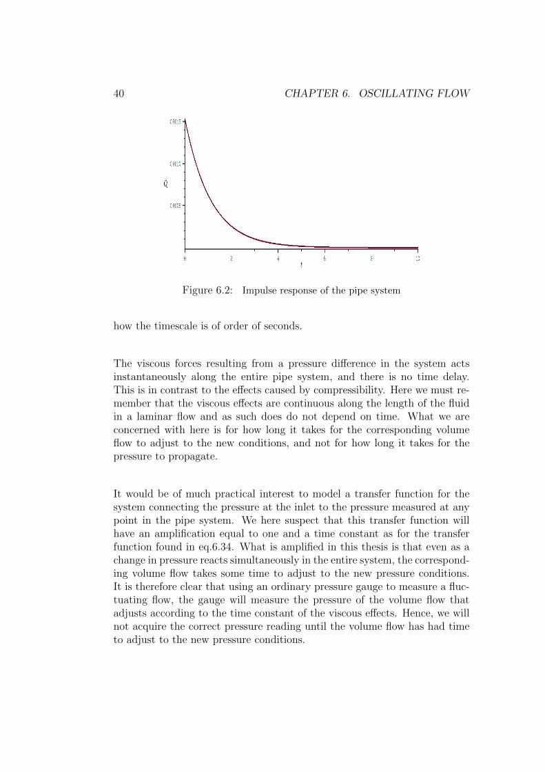
Figure 6.2 shows the impulse response of the pipe system. We have chosenthe values ∆p = 1 [Pa], a = 1 [cm], l = 10 [cm] and used the characteristicsof air.13 The response is given in time as the corresponding volume flowfollowing a unit size change of the pressure in form of an impulse. We note

12We here refer to [3] B. P. Lathi ’Linear Systems and Signals’13These values will be used further on as both the frequency- and step response are

illustrated.


Figure 6.2: Impulse response of the pipe system

how the timescale is of order of seconds.

The viscous forces resulting from a pressure difference in the system actsinstantaneously along the entire pipe system, and there is no time delay.This is in contrast to the effects caused by compressibility. Here we must re-member that the viscous effects are continuous along the length of the fluidin a laminar flow and as such does do not depend on time. What we areconcerned with here is for how long it takes for the corresponding volumeflow to adjust to the new conditions, and not for how long it takes for thepressure to propagate.

It would be of much practical interest to model a transfer function for thesystem connecting the pressure at the inlet to the pressure measured at anypoint in the pipe system. We here suspect that this transfer function willhave an amplification equal to one and a time constant as for the transferfunction found in eq.6.34. What is amplified in this thesis is that even as achange in pressure reacts simultaneously in the entire system, the correspond-ing volume flow takes some time to adjust to the new pressure conditions.It is therefore clear that using an ordinary pressure gauge to measure a fluc-tuating flow, the gauge will measure the pressure of the volume flow thatadjusts according to the time constant of the viscous effects. Hence, we willnot acquire the correct pressure reading until the volume flow has had timeto adjust to the new pressure conditions.


6.3.2 Frequency response


For an harmonic function of a single frequency, for which the transform yieldsa pole in ωm = ω0 + iε in the upper half plane, we have that

u(r, t) =1

πρl

(∑k

Res[f(ω) lim

ε→0

∆pε

(ω − ω0)2 + ε2, ωk]

+Res[f(ω) lim

ε→0

∆pε

(ω − ω0)2 + ε2, ωm

]). (6.35)

We realize that this is calculated as

u(r, t) =G(r, t)

πρllimε→0

∑k

ε∆p

((ω − ω0)2 − ε2)

∣∣∣∣∣ω=iν

J20,k

a2

+1

πρllimε→0

ε∆p

((ω − ω0) + iε)ω

(1−

J0(r√−iων

)J0(a√−iων

))eiωt

∣∣∣∣∣ω=ω0+iε

. (6.36)

As the first factor of eq. (6.36) clearly approaches zero in the limit ε→ 0, itis sufficient to only consider the last factor as we continue.

u(r, t) =1

πρllimε→0

ε∆p

(ω0 + iε)((ω0 + iε− ω0) + iε)

(1−

J0(r√−i(ω0+iε)

ν

)J0(a√−i(ω0+iε)

ν

))ei(ω0+iε)t

=1

πρllimε→0

ε∆p

(ω0 + iε)(2iε)

(1−

J0(r√−i(ω0+iε)

ν

)J0(a√−i(ω0+iε)

ν

))ei(ω0+iε)t, (6.37)

which yields the solution14

u(r, t) =−i∆p2πρlω0

(1−

J0(r√−iω0

ν

)J0(a√−iω0

ν

))eiω0t. (6.38)

14This result is in accordance to the solution given by Per Amund Amundsen in hisunpublished note concerning ’Oscillating flow in a pipe’



The frequency volume response of the system becomes

Q(t) = 2π

∫ a

0

r−i∆p2πρω0l

(1−

J0(r√−iω0

ν

)J0(a√−iω0

ν

))eiω0tdr

=−i∆pa2

16ρlω0

eiω0t

(J2(a

√−iω0

ν)

J0(a√−iω0

ν)

). (6.39)

Eq. 6.39 represents the frequency response of a pipe filled with fluid as weconsider the viscous effects only. As we further define

Q(t) = Q0eiw0t and ∆p(t) = ∆p0e

iw0t, (6.40)

we can express the frequency response as a transfer function relating thepressure and the volume flow in the pipe system15

H(ω) =Q0

∆p0= <

[−ia2

16ρlω

(J2(a

√−iων

)

J0(a√−iων

)

)]. (6.41)

The real part of eq. 6.41 can be found from the relation Jn(√−iz) =

(−1)n(bern(z)− ibein(z)), where bern(z) and bein(z) are Kelvin functions16.

H(ω) = <

[−i∆pa2

16ρlω

(ber2(a

√ων)− ibei2(a

√ων)

ber0(a√

ων)− ibei0(a

√ων)

)]

=∆pa2

16ρlω

(ber2(a

√ων)bei0(a

√ων)− ber0(a

√ων)bei2(a

√ων)

ber20(a√

ων) + bei20(a

√ων)

). (6.42)

We now have that given an input in the form of a harmonically oscillatingpressure function the resulting velocity profile in the pipe is

cos(ωt+ φ)⇒ H(ω) cos(ωt+ φ). (6.43)

15We here refer to [3] B. P. Lathi ’Linear Systems and Signals’16We here refer to [7] Frank W. Olver, Danile W. Lozier, Ronald F. Boisvert and Charles

W. Clark ’Nist handbook of mathematical functions’


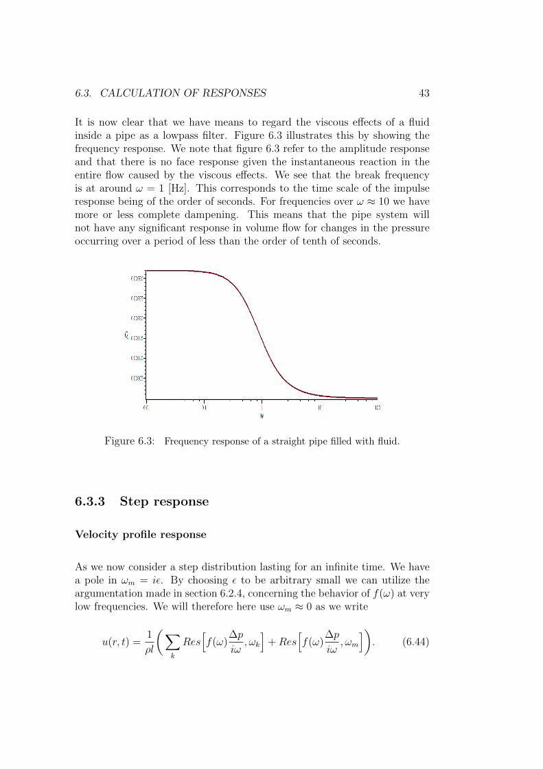
It is now clear that we have means to regard the viscous effects of a fluidinside a pipe as a lowpass filter. Figure 6.3 illustrates this by showing thefrequency response. We note that figure 6.3 refer to the amplitude responseand that there is no face response given the instantaneous reaction in theentire flow caused by the viscous effects. We see that the break frequencyis at around ω = 1 [Hz]. This corresponds to the time scale of the impulseresponse being of the order of seconds. For frequencies over ω ≈ 10 we havemore or less complete dampening. This means that the pipe system willnot have any significant response in volume flow for changes in the pressureoccurring over a period of less than the order of tenth of seconds.

Figure 6.3: Frequency response of a straight pipe filled with fluid.

6.3.3 Step response


As we now consider a step distribution lasting for an infinite time. We havea pole in ωm = iε. By choosing ε to be arbitrary small we can utilize theargumentation made in section 6.2.4, concerning the behavior of f(ω) at verylow frequencies. We will therefore here use ωm ≈ 0 as we write

u(r, t) =1

ρl

(∑k

Res[f(ω)

∆p

iω, ωk

]+Res

[f(ω)

∆p

iω, ωm

]). (6.44)


We substitute eq. 6.27 and eq. 6.21 into eq. 6.44 and as such we have

u(r, t) =∑k

∆p

iωG(r, t)

∣∣∣∣∣w=iν

j20,k

a2

+∆p

if(0), (6.45)

which yields

u(r, t) = ∆p

((a2 − r2)

4ρlν− 2a2

ρlν

∑k

1

j30,k

(J0(rajo,k)

J1(jo,k) )e−( j0,ka )2νt). (6.46)

We now have the transient and everlasting term of the flow resulting from apressure change in the from of a step described separately in eq. 6.46. Wesee that as the time t increases the flow approach the Possuille-Hagen profilefor the flow as expected.

From a mathematical point of view it is worth noticing that as the flow mustbe zero at t = 0, the two terms making up eq. 6.46 must yield the samevalue at that instant. Hence, we have by chance found the sum of the Besselfunctions zeros when presented as in eq. 6.46. We have that

∑k

j0,k

(J0(rajo,k)

J1(jo,k) )e−( j0,ka )2νt =

(a2 − r2)8a2

. (6.47)


The step response of the system can be found as

Q(t) = 2π

(∫ a

0

r(a2 − r2)

4ρlνdr − 2a2

ρlν

∑k

1

j30,ke−(j0,ka

)2νt

∫ a

0

r

(J0(rajo,k)

J1(jo,k) )dr

= 2π

(a4

16ρlν− 2a4

ρlν

∑k

1

j40,ke−(j0,ka

)2νt

)

=4πa4

ρlν

(1

32−∑k

1

j40,ke−(j0,ka

)2νt

). (6.48)


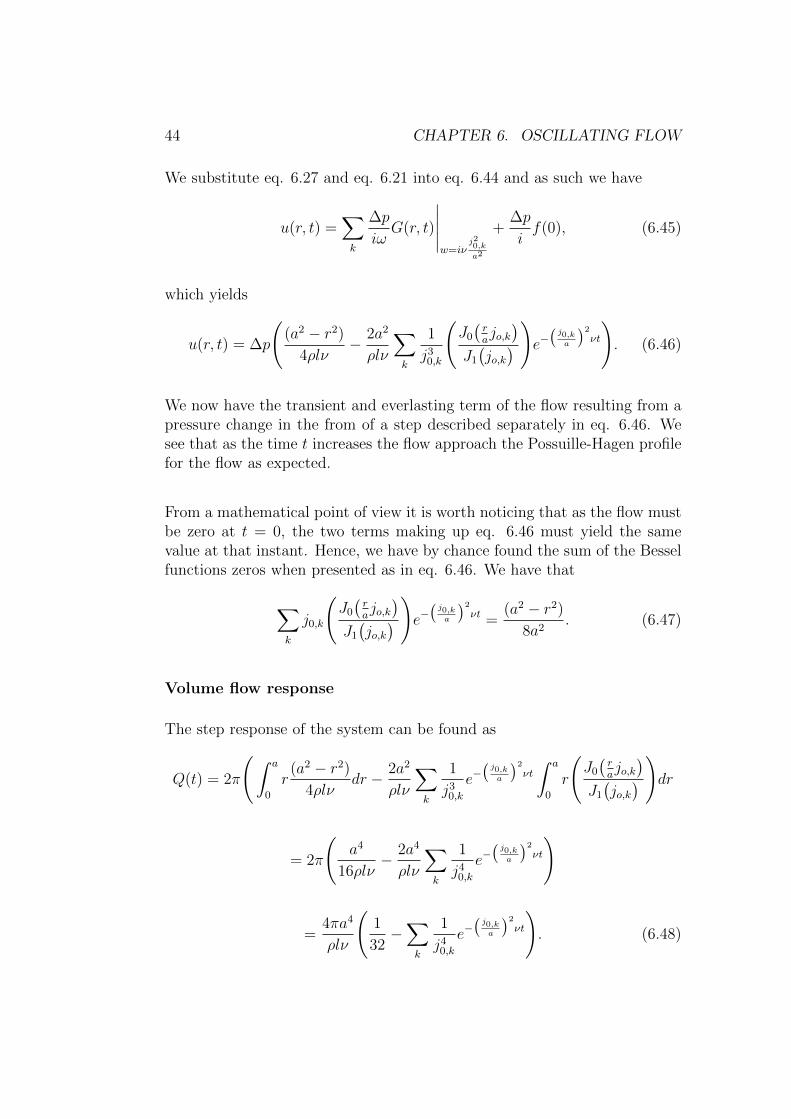
with∑

k j0,k = 2.5 we have in the Laplace domain

1

sHp(s) ≈

4πa4

ρlν

(1

32−

a2

230νa2

6νs+ 1

). (6.49)

Figure 6.4: Step response of the pipe system.

We see from figure 6.4 that the step response here corresponds with theimpulse and frequency response. As we previously have calculated both theimpulse and frequency response of the system it might seem excessive to havecalculated the step response in addition. We have done this in an attemptto wheel this thesis in the direction of the field of control systems, where thestep response is a more common representation of the systems characteristicsthan the impulse response. Another reason for including the step response isthat we during the calculation have stumbled upon a way of finding the sumof the zeros of the Bessel functions. It is unfortunate that there will not beroom to pursue this discovery further. If some one where to pick up the traceleft behind here it would be interesting to see whether it is possible to findother expressions for the zeros of the Bessel function, or similar functions,by exiting the system to other functions.

Chapter 7

Conclusion

From the above chapters the system can now be described as a circularjet entering a quiescent fluid which after a transition zone can be modeledas a non-viscous flow described by its mean velocity. This we presume re-mains valid in the contracting part of the pipe system as well as for the twopipes. The above results also demonstrate how the velocity profile and thecorresponding volume flow of a stream changes according to changes of thepressure in the pipe system. From this we find the means to express the pipesystem as a transfer function. These results also apply to the narrow shaftwhich the air passes through as some of it leaks out of the pipe system toreach the pressuregauge.

We see that the pressuregauge is not measuring the actual pressure in thepipe system, but the pressure of the corresponding volume flow adjustingto the pressure change in the pipe system. We find that this change occursover a period of seconds, and that it depends on the maximal radius of thepipe and the viscosity of the fluid. We find that the effects caused by viscos-ity dominates over the effects caused by compressibility, and as we presumeother effects to be even less significant we argue a model of the pipe systembased on the viscous effects only.

The entire system, containing both the pipe system and the measuring ar-rangement, should be regarded as two separate transfer functions in connec-tion. They will both be governed by the same viscous forces, but will have adifferent diameter of the pipe and hence a different time constant. We havethat the time constant of the viscous effects increase with the maximal radiusof the pipe in the second order, as such the time constant of the pipe system

47

48 CHAPTER 7. CONCLUSION

will dominate the time constant of the measuring arrangement. Hence, wemight discard the time constant associated with the measuring arrangement.

From the frequency response of the system it can be seen that the systemacts as a lowpass filter. The viscous forces within the fluid dampens out highfrequency changes of the inlet pressure. The physical explanation for this isthat the fluid particles takes some time to react to new pressure conditionsbecause of the viscous forces between them. Hence, rapid fluctuations willin an increasing manner be dampened out.

The model of the stationary turbulent flow is mainly an argument for notconsidering the thickness of the boundary layers under steady conditions.We are reminded that this might not be valid for a fluctuating flow, andthat there might be reason for special concern during starting and closingprocedures.

It is important to remember that the discussions made in this thesis doesnot directly apply to the real system under consideration. We have not con-sidered in detail the sonic conditions and effects on the boundary layer thatmight appear at the inlet of the system. The solution for the jet and the time-dependent solution applies to a laminar flow and we have not considered howto extend these solutions in the case of turbulence and roughness in the pipethat exceeds the hight of the laminar boundary layer. Neither can we becertain to what degree the effects caused by compressibility and turbulencecan be regarded as linear with respect to the viscous effects. There are un-doubtedly other concerns regarding the model that could have been examinedin more detail and we are reminded that this model is to be considered crude.

This thesis has clarified a mathematical model that can be used in the designof an automatic control system that has the ability to regulate the volumeflow through the pipe system similar to the one we have discussed here. Itshould be notes that all the solutions we have arrived at in this thesis is basedon pure mathematical and physical assumptions, and that there has been nosimulation or testing involved. It could therefore have valuable contributionsfrom computer simulation, such as FEM, and from visualization of the actualphenomena, by for example the means of electrolysis and a transparent pipe.

Chapter 8

References

1. D. J. Tritton; Physical Fluid Dynamics 2. ed. OPU, Oxford 1988.

2. Pijush K. Kundu, Ira M. Cohen and David R. Dowling; Fluid Mechanics5. ed. Elsevier 2012.

3. B. P. Lathi; Linear Systems and Signals 2. ed. Oxford University Press2010.

4. George Arfken; Mathematical Methods for Physicists 2. ed. AcademicPress 1968.

5. Eugen Butkov; Mathematical Physics 1. ed. Addison-Wesley PublishingCompany 1968.

6. Per Amund Amundsen; Occilating laminar flow in a pipe. Unpublishednote.

7. Frank W. Olver, Danile W. Lozier, Ronald F. Boisvert and Charles W.Clark; Nist handbook of mathematical functions. Cambridge University Press2010.

8. Maplesoft; Maple 16. Computer program used for some of the calculationsand to draw the graphs.

49

modeling of the viscous e ects in uids - core.ac.uk · @y = 1 ˆ @p 0 @z + @2u @y2 ... ira m. cohen...

Documents