fluid mechanics kundu cohen 6th edition solutions sm ch (14)

Fluid Mechanics, 6th Ed. Kundu, Cohen, and Dowling

Exercise 14.1. As an extension of Example 14.1, consider a sphere with radius a that moves along the x-axis on a trajectory given by xp(t) = xp(t)ex in a fluid moving with uniform velocity: u = Uex + Vey. Determine a formula for the mechanical power, W, necessary to overcome the aerodynamic drag force on the sphere in terms of a, U, V, xp, ρ = the density of the air, and CD = the drag coefficient of the sphere. If dxp/dt is constant, under what conditions is W reduced by the presence of non-zero u? Solution 14.1. The drag force magnitude will depend on the square of the relative velocity between the sphere and the fluid. The drag force direction will be parallel to the relative velocity of the sphere and the fluid. The relative velocity is the fluid velocity observed when riding on the sphere. If the fluid velocity is u = (U,V), then Vrel = U − dxp dt( )ex +Vex , so the drag force vector is:

D = ρ πa2

2CD U − dxp dt( )

2+V 2 U − dxp dt( )ex +Vex"# $% .

When the sphere is stationary, then D points in the same direction as U. When the fluid is stationary D points in the opposite direction of dxp/dt; it opposes the motion of the sphere. From Newton's third law, the force applied to the fluid by the motive mechanism of the sphere to overcome the drag force is –D. The power output of this force is:

W = −D ⋅dxpdtex

#

$%

&

'(= −ρ

πa2

2CD U − dxp dt( )

2+V 2 U − dxp dt( ) dxp dt( ) .

When the fluid velocity is zero, then the power is:

Wo = ρπa2

2CD dxp dt( )

3 .

To find out when non-zero u reduces W, first determine the boundary where W = Wo

ρπa2

2CD dxp dt( )

3= −ρ

πa2

2CD U − dxp dt( )

2+V 2 U − dxp dt( ) dxp dt( ) .

Divide out common factors, and define normalized fluid velocities: !U =U

dxp dt and !V =

Vdxp dt

to reach: 1= − !U −1( )2+ !V 2 !U −1( ) .

Rearrange and square to eliminate the square root, then solve for !V 1!U −1( )

2 = !U −1( )2+ !V 2 which implies: !V 2 =

1!U −1( )

2 − !U −1( )2=

1!U −1( )

2 1− !U −1( )4( ) .

Take the square root and factor inside of the last set of parentheses:

!V = ±1!U −1( )

1− !U −1( )2"

#$%&'1+ !U −1( )

2"#$

%&'

()*

+,-1 2

= ±1!U −1( )

2 !U − !U 2"# %& !U2 + 2 !U + 2"# %&( )

1 2 .

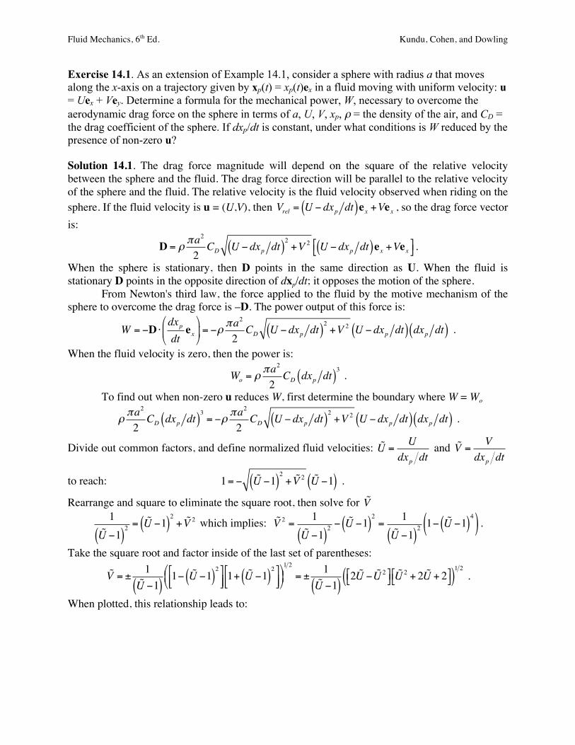
When plotted, this relationship leads to:


where the area inside the four-lobed contour is where W < Wo.

!10$

!8$

!6$

!4$

!2$

0$

2$

4$

6$

8$

10$

0$ 0.25$ 0.5$ 0.75$ 1$ 1.25$ 1.5$ 1.75$ 2$

!V

!U


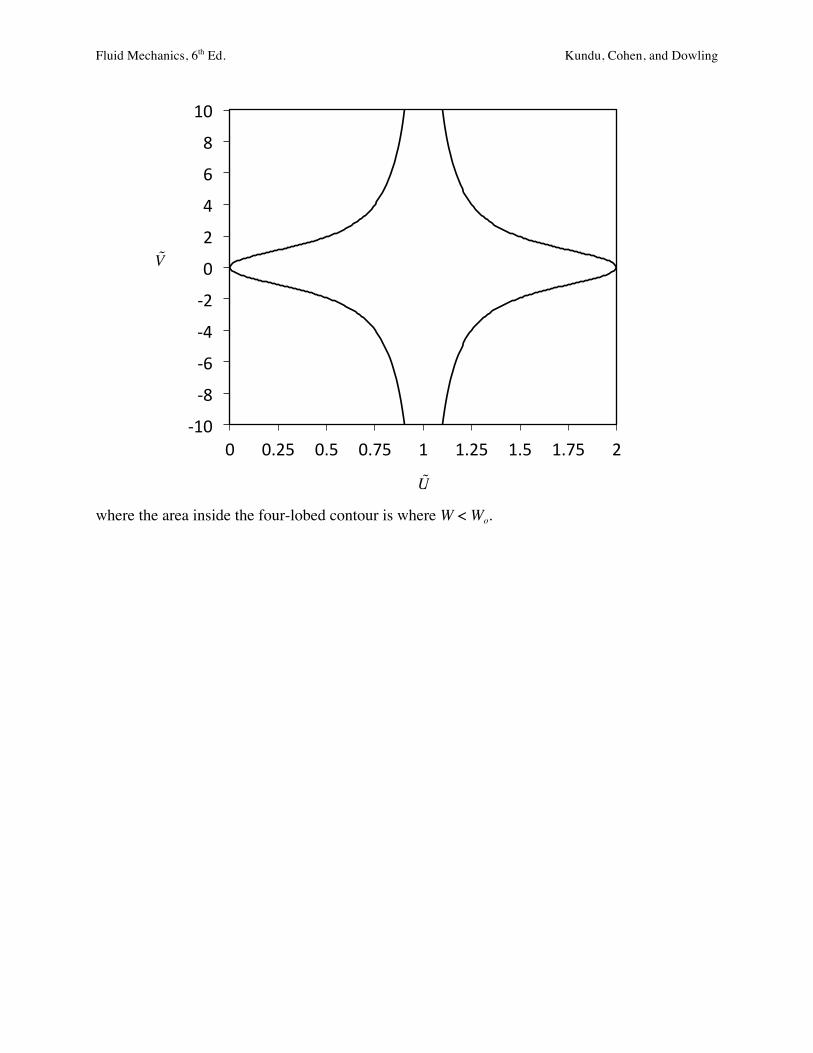
Exercise 14.2. Consider the elementary aerodynamics of a projectile of mass m with CL = 0 and CD = constant. In Cartesian coordinates with gravity g acting downward along the y-axis, a set of equations for such a projectile's motion are:

€

m dVx

dt= −Dcosθ ,

€

mdVy

dt= −mg−Dsinθ ,

€

tanθ =Vy Vx , and

€

D =12ρ Vx

2 +Vy2( )ACD ,

where Vx and Vy are the horizontal and vertical components of the projectile's velocity, θ is the angle of the projectile's trajectory with respect to the horizontal, D is the drag force on the projectile, ρ is the air density, and A is projectile's frontal area. Assuming a shallow trajectory, where

€

Vx2 >>Vy

2 and

€

mg >> Dsinθ , show that the distance traveled by the projectile over level

ground is:

€

x ≅ 2mρACD

ln 1+ρACDVo

2 cosθo sinθomg

%

& '

(

) * if it is launched from ground level with speed

of Vo at an angle of θo with respect to the horizontal. Does this answer make sense as

€

CD → 0?

Solution 14.2. Insert the approximations in the horizontal and vertical equations of motion to find:

€

m dVx

dt≅ −

12ρVx

2ACD , and

€

mdVy

dt≅ −mg.

Here it has been assumed that the trajectory is shallow enough so that cosθ is approximately unity on the projectile's trajectory. The initial conditions are Vx = Vocosθo and Vy = Vosinθo at t = 0. Both equations can be integrated once to find:

€

−1Vx2∫ dVx ≅

ρACD

2mdt∫ or

€

1Vx

=ρACD

2mt + C1, and

€

m dVy = −mg∫ dt∫ or

€

Vy ≅ C2 − gt .

where C1 and C2 are constants that can be evaluated with the initial conditions to reach:

€

1Vx

≅ρACD

2mt +

1Vo cosθo

, and

€

Vy ≅Vo sinθo − gt .

To find the approximate position of the projectile, these equations for the velocity components must be integrated again using Vx = dx/dt and Vy = dy/dt with initial conditions x = 0 and y = 0 at t = 0. The horizontal coordinate equation can be rearranged and integrated,

€

1Vx

=dtdx

≅ρACD

2mt +

1Vo cosθo

,

€

Vo cosθodt

ρACDVo cosθo 2m( )t +1∫ ≅ dx∫ ,

to find:

€

x ≅ 2mρACD

ln 1+ρACDVo cosθo

2mt

%

& '

(

) * + C3.

The initial condition leads to C3 = 0. The vertical coordinate equation can be integrated directly:


€

Vy =dydt

≅Vo sinθo − gt or

€

y ≅Vot sinθo −12gt 2 + C4 .

and the initial condition again leads to C4 = 0. The time, tf, the projectile is in flight over level ground can be determined from the vertical coordinate equation by looking for the second time y = 0:

€

y = 0 ≅Vot f sinθo −12gt f

2 , which implies: tf = 0 , or

€

t f ≅2Vo sinθo

g.

Substituting this time into the horizontal coordinate equation determines the projectile's horizontal location when it hits the ground:

€

x ≅ 2mρACD

ln 1+ρACDVo

2 cosθo sinθomg

%

& '

(

) * .

When

€

CD → 0 the frictionless mechanics solution should be recovered. Using the expansion of the natural logarithm, ln(1 + ε) = ε + ... for ε << 1, the above equation becomes:

€

x ≅ 2mρACD

ρACDVo2 cosθo sinθomg

=2Vo

2 cosθo sinθog

,

which is correct when the projectile flies in vacuum. Although the main result of this exercise is approximate, it does incorporate the physically important feature that aerodynamic drag decreases projectile travel distances in still air.


Exercise 14.3. As a model of a two-dimensional airfoil's trailing edge flow consider the potential

€

φ(r,θ) = Ud n( ) r d( )n cos nθ( ) in the usual r-θ coordinates (Figure 3.3a). Here U, d, and n are positive constants, the fluid has density ρ, and the foil's trailing edge lies at the origin of coordinates. a) Sketch the flow for n = 3/2, 5/4, and 9/8 in the angle range |θ| < π/n, and determine the full included angle of the foil's trailing edge in terms of n. b) Determine the fluid velocity at r = d and θ = 0. c) If p0 is the pressure at the origin of coordinates and pd is the pressure at r = d and θ = 0, determine the pressure coefficient:

€

Cp = (p0 − pd )12 ρU

2( ) as a function of n. In particular, what is Cp when n = 1 and when n > 1? Solution 14.3. a) The velocity components in this flow are:

€

ur =∂∂rφ =

Udnn r

n−1

dncos(nθ) =U r

d&

' ( )

* + n−1

cos(nθ) , and

€

uθ =1r∂∂θ

φ =Udnrn−1

dn−n( )sin(nθ) = −U r

d&

' ( )

* + n−1

sin(nθ) .

The angular velocity is zero at: θ = 0, ± π/n. The radial velocity is positive on θ = 0, but negative on θ = ± π/n. Thus, the full included angle of the foil's trailing edge is 2(π – π/n) = 2π(n – 1)/n, and this angle decreases toward zero as

€

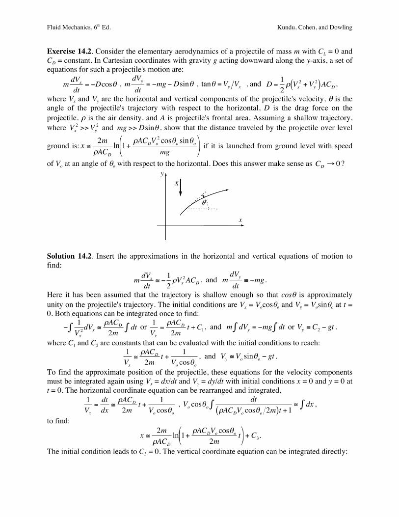
n→1. For n = 3/2, the full included angle of the foil's trailing edge is = 2π(3/2 – 1)/(3/2) = 2π/3 (120°).

For n = 5/4, the full included angle of the foil's trailing edge is = 2π(5/4 – 1)/(5/4) = 2π/5 (72°).

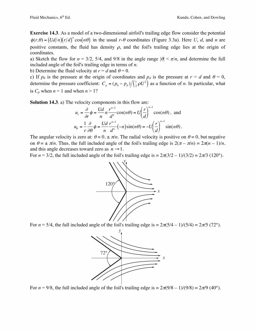
For n = 9/8, the full included angle of the foil's trailing edge is = 2π(9/8 – 1)/(9/8) = 2π/9 (40°).

x

y

120°

x

y

72°


b) From the velocity results provided above in part a), the fluid velocity at r = d and θ = 0 is:

€

ur(d,0) =U dd"

# $ %

& ' n−1

cos(0) = +U , and

€

uθ (d,0) = −U dd$

% & '

( ) n−1

sin(0) = 0 .

c) To determine the coefficient of pressure, use the steady-flow Bernoulli equation without the body-force term:

€

p +12ρ ur

2 + uθ2( )$

% & '

( ) r= 0= p +

12ρ ur

2 + uθ2( )$

% & '

( ) r= d ,θ = 0

,

and evaluate:

€

p0 + limr→0

12ρ U 2 r

d$

% & '

( ) 2n−2

cos2(nθ) +U 2 rd$

% & '

( ) 2n−2

sin2(nθ)$

% & &

'

( ) ) = pd +

12ρ U 2 + 0( ) .

Simplify and rearrange:

€

p0 − pd =12ρU 2 1− lim

r→0

rd%

& ' (

) * 2n−2%

& ' '

(

) * * , or

€

Cp =1− limr→0

rd$

% & '

( ) 2(n−1)

.

Therefore:

€

Cp =

1 for n >10 for n =1−∞ for n <1

$

% &

' &

(

) &

* &

.

This result shows that there is a stagnation point at a foil's trailing edge when the trailing-edge included angle is non-zero.

x

y

40°


Exercise 14.4. Consider an airfoil section in the xy-plane, the x-axis being aligned with the chord line. Examine the pressure forces on an element ds = (dx, dy) on the surface, and show that the net force (per unit span) in the y-direction is

€

Fy = − pudx0

c∫ + pldx0

c∫

where pu and p1 are the pressure on the upper and the lower surfaces and c is the chord length. Show that this relation can be rearranged in the form

€

Cy =Fy

(1/2)ρU 2c= Cpd

xc#

$ % &

' ( ∫ ,

where

€

Cp = (p0 − p∞)12 ρU

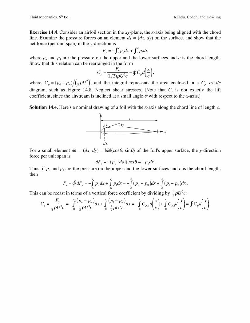
2( ) , and the integral represents the area enclosed in a Cp vs x/c diagram, such as Figure 14.8. Neglect shear stresses. [Note that Cy is not exactly the lift coefficient, since the airstream is inclined at a small angle α with respect to the x-axis.] Solution 14.4. Here's a nominal drawing of a foil with the x-axis along the chord line of length c.

For a small element ds = (dx, dy) = |ds|(cosθ, sinθ) of the foil's upper surface, the y-direction force per unit span is

€

dFy = −(pu | ds |)cosθ = −pudx . Thus, if pu and p1 are the pressure on the upper and the lower surfaces and c is the chord length, then

€

Fy = dFy = − pu0

c

∫ dx∫ + pl0

c

∫ dx = − pu − p∞( )0

c

∫ dx + pl − p∞( )0

c

∫ dx .

This can be recast in terms of a vertical force coefficient by dividing by

€

12 ρU

2c :

€

Cy =Fy

12 ρU

2c= −

pu − p∞( )12 ρU

2c0

c

∫ dx +pl − p∞( )12 ρU

2c0

c

∫ dx = − Cp,u0

c

∫ d xc&

' ( )

* + + Cp,l

0

c

∫ d xc&

' ( )

* + = Cp∫ d x

c&

' ( )

* + .

dx

y

!ds

x

c


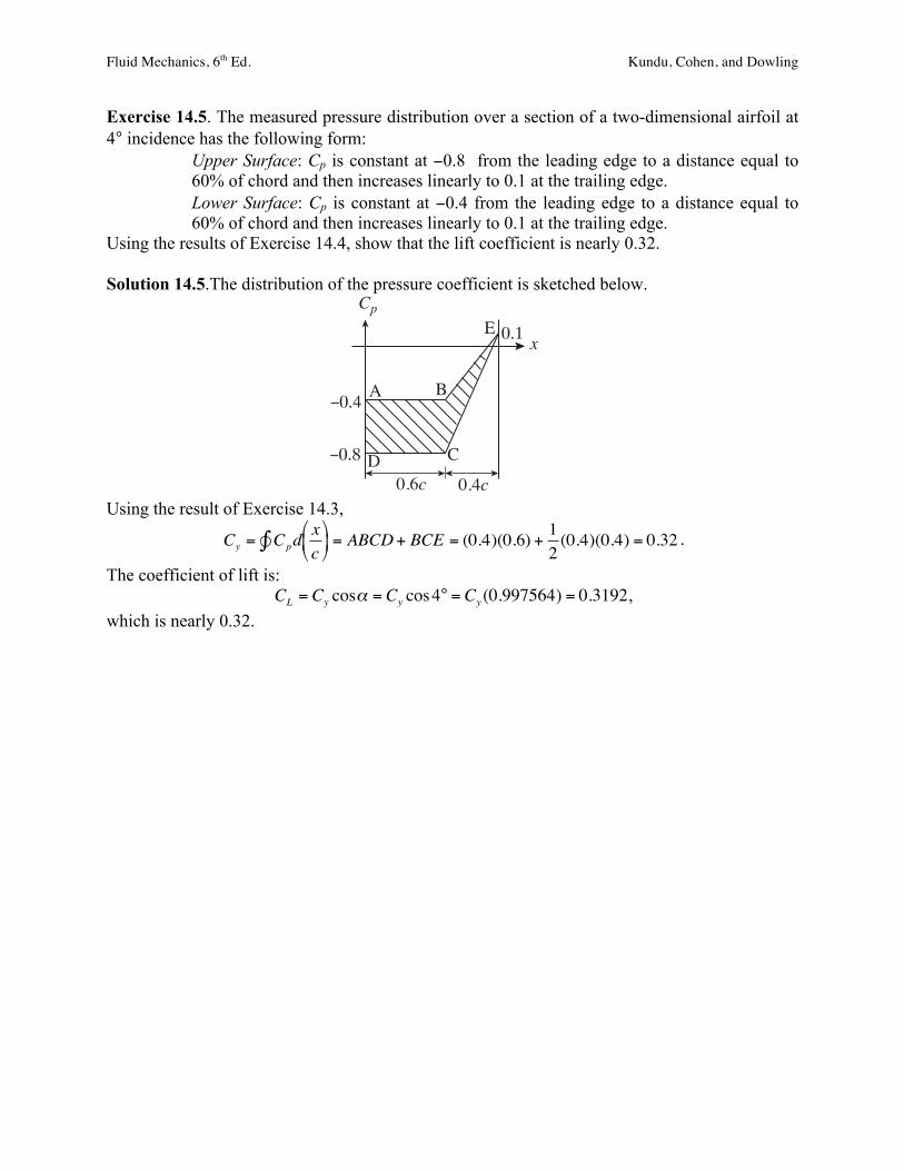
Exercise 14.5. The measured pressure distribution over a section of a two-dimensional airfoil at 4° incidence has the following form:

Upper Surface: Cp is constant at −0.8 from the leading edge to a distance equal to 60% of chord and then increases linearly to 0.1 at the trailing edge. Lower Surface: Cp is constant at −0.4 from the leading edge to a distance equal to 60% of chord and then increases linearly to 0.1 at the trailing edge.

Using the results of Exercise 14.4, show that the lift coefficient is nearly 0.32. Solution 14.5.The distribution of the pressure coefficient is sketched below.

Using the result of Exercise 14.3,

€

Cy = Cp∫ d xc#

$ % &

' ( = ABCD+ BCE = (0.4)(0.6) +

12(0.4)(0.4) = 0.32 .

The coefficient of lift is:

€

CL = Cy cosα = Cy cos4° = Cy (0.997564) = 0.3192, which is nearly 0.32.

–!"#

–!"$

!"%

0.4c0.6c

x

Cp

A B

E

CD


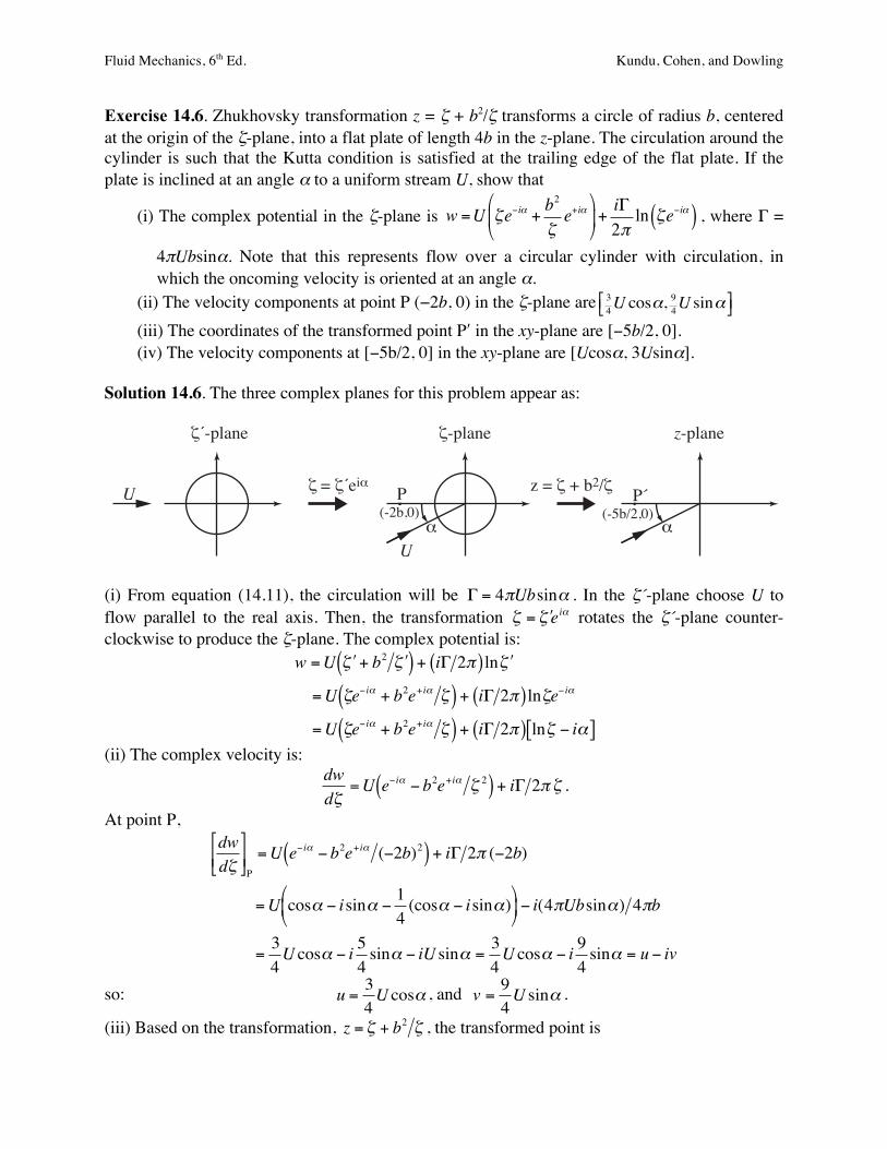
Exercise 14.6. Zhukhovsky transformation z = ζ + b2/ζ transforms a circle of radius b, centered at the origin of the ζ-plane, into a flat plate of length 4b in the z-plane. The circulation around the cylinder is such that the Kutta condition is satisfied at the trailing edge of the flat plate. If the plate is inclined at an angle α to a uniform stream U, show that

(i) The complex potential in the ζ-plane is w =U ζe−iα + b2

ζe+iα

"

#$

%

&'+

iΓ2πln ζe−iα( ) , where Γ =

4πUbsinα. Note that this represents flow over a circular cylinder with circulation, in which the oncoming velocity is oriented at an angle α.

(ii) The velocity components at point P (−2b, 0) in the ζ-plane are 34U cosα,

94U sinα!" #$

(iii) The coordinates of the transformed point Pʹ′ in the xy-plane are [−5b/2, 0]. (iv) The velocity components at [−5b/2, 0] in the xy-plane are [Ucosα, 3Usinα].

Solution 14.6. The three complex planes for this problem appear as:

(i) From equation (14.11), the circulation will be

€

Γ = 4πUbsinα . In the ζ´-plane choose U to flow parallel to the real axis. Then, the transformation

€

ζ = # ζ eiα rotates the ζ´-plane counter-clockwise to produce the ζ-plane. The complex potential is:

€

w =U " ζ + b2 " ζ ( ) + iΓ 2π( ) ln " ζ

=U ζe−iα + b2e+iα ζ( ) + iΓ 2π( ) lnζe− iα

=U ζe−iα + b2e+iα ζ( ) + iΓ 2π( ) lnζ − iα[ ]

(ii) The complex velocity is:

€

dwdζ

=U e−iα − b2e+iα ζ 2( ) + iΓ 2π ζ .

At point P,

€

dwdζ#

$ % &

' ( P=U e−iα − b2e+iα (−2b)2( ) + iΓ 2π (−2b)

=U cosα − isinα − 14

(cosα − isinα)-

. /

0

1 2 − i(4πUbsinα) 4πb

=34U cosα − i 5

4sinα − iU sinα =

34U cosα − i 9

4sinα = u − iv

so:

€

u =34U cosα , and

€

v =94U sinα .

(iii) Based on the transformation,

€

z = ζ + b2 ζ , the transformed point is

!´-plane

! = !´ei"U

!-plane

U

"

z-plane

P(-2b,0)

P´(-5b/2,0)

z = !#+ b2/!

"


€

z " P = −2b + b2 (−2b) = −5b /2 . (iv) The complex velocity at (–5b/2, 0) in the z-plane is:

€

dwdz

=dwdζ

dζdz

=dwdζ

dzdζ#

$ %

&

' (

−1

=dwdζ

1− b2

ζ 2

#

$ %

&

' (

−1

=dwdζ

ζ 2

ζ 2 − b2

#

$ %

&

' (

=34U cosα − i 9

4sinα

#

$ %

&

' (

(−2b)2

(−2b)2 − b2

#

$ %

&

' ( =U cosα − i3sinα = u − iv.

where ζ = (–2b, 0) has been used as the corresponding point in the ζ-plane.


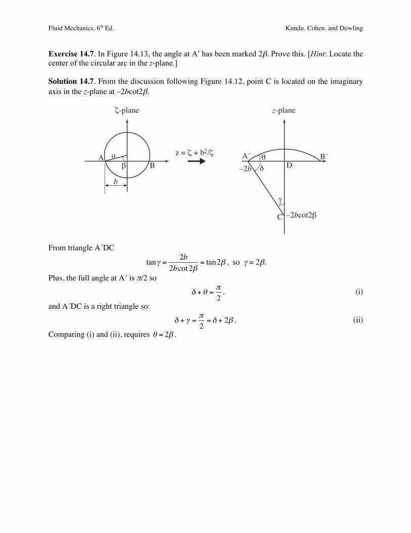
Exercise 14.7. In Figure 14.13, the angle at Aʹ′ has been marked 2β. Prove this. [Hint: Locate the center of the circular arc in the z-plane.] Solution 14.7. From the discussion following Figure 14.12, point C is located on the imaginary axis in the z-plane at –2bcot2β.

From triangle A´DC

€

tanγ =2b

2bcot 2β= tan2β , so γ = 2β.

Plus, the full angle at A´ is π/2 so

€

δ + θ =π2

, (i)

and A´DC is a right triangle so:

€

δ + γ =π2

= δ + 2β . (ii)

Comparing (i) and (ii), requires

€

θ = 2β .

!-plane

D

z-plane

z = !"+ b2/!A

B#

a A´ B´$

%

&

b

–2b

C –2bcot2#


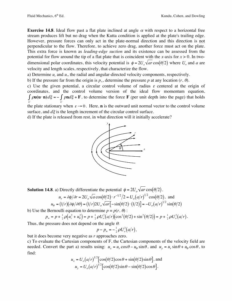
Exercise 14.8. Ideal flow past a flat plate inclined at angle α with respect to a horizontal free stream produces lift but no drag when the Kutta condition is applied at the plate's trailing edge. However, pressure forces can only act in the plate-normal direction and this direction is not perpendicular to the flow. Therefore, to achieve zero drag, another force must act on the plate. This extra force is known as leading-edge suction and its existence can be assessed from the potential for flow around the tip of a flat plate that is coincident with the x-axis for x > 0. In two-dimensional polar coordinates, this velocity potential is

€

φ = 2Uo ar cos θ 2( ) where Uo and a are velocity and length scales, respectively, that characterize the flow. a) Determine ur and uθ, the radial and angular-directed velocity components, respectively. b) If the pressure far from the origin is p∞, determine the pressure p at any location (r, θ). c) Use the given potential, a circular control volume of radius ε centered at the origin of coordinates, and the control volume version of the ideal flow momentum equation,

€

ρu(u ⋅n)dξ =C∫ − pndξ

C∫ + F , to determine the force F (per unit depth into the page) that holds

the plate stationary when

€

ε → 0 . Here, n is the outward unit normal vector to the control volume surface, and dξ is the length increment of the circular control surface. d) If the plate is released from rest, in what direction will it initially accelerate?

Solution 14.8. a) Directly differentiate the potential

€

φ = 2Uo ar cos θ 2( ) .

€

ur = ∂φ ∂r = 2Uo a cos θ 2( ) ⋅ r−1 2 2 =Uo a r( )1 2 cos θ 2( ), and

€

uθ = 1 r( ) ∂φ ∂θ( ) = 1 r( )2Uo ar −sin θ 2( ) ⋅ 1 2( )[ ] = −Uo a r( )1 2 sin θ 2( ) b) Use the Bernoulli equation to determine p = p(r, θ) :

€

p∞ = p + 12 ρ ur

2 + uθ2( ) = p + 1

2 ρUo2 a r( ) cos2 θ 2( ) + sin2 θ 2( )( ) = p + 1

2 ρUo2 a r( ) .

Thus, the pressure does not depend on the angle θ:

€

p − p∞ = − 12 ρUo

2 a r( ), but it does become very negative as r approaches zero. c) To evaluate the Cartesian components of F, the Cartesian components of the velocity field are needed. Convert the part a) results using:

€

ux = ur cosθ − uθ sinθ , and

€

uy = ur sinθ + uθ cosθ , to find:

€

ux =Uo a r( )1 2 cos θ 2( )cosθ + sin θ 2( )sinθ[ ], and

€

uy =Uo a r( )1 2 cos θ 2( )sinθ − sin θ 2( )cosθ[ ] .


These can be simplified to:

€

ux =Uo a r( )1 2 cos θ 2( ) , and

€

uy =Uo a r( )1 2 sin θ 2( ) , using trigonometric identities. Here

€

n = er = ex cosθ + ex sinθ , so

€

u ⋅n = u ⋅ er = ur. Thus, the CV equation can be written in terms of x- and y-components:

€

ρ uxex + uyey( )urεdθ0

2π∫ = − p(ex cosθ + ex sinθ)εdθ0

2π∫ + Fxex + Fyey .

where dξ = εdθ. The pressure does not depend on θ, and the integrals of cosθ and sinθ from 0 to 2π are both zero so the pressure integration drops out leaving:

€

ρ Uo a ε( )1 2 cos θ 2( )( )Uo a ε( )1 2 cos θ 2( )εdθ0

2π∫ = Fx , and

€

ρ Uo a ε( )1 2 sin θ 2( )( )Uo a ε( )1 2 cos θ 2( )εdθ0

2π∫ = Fy .

The ε contour-radius factors cancel, so the integrands can be simplified to:

€

ρUo2a cos2 θ 2( )dθ0

2π∫ = Fx , and

€

ρUo2a sin θ 2( )cos θ 2( )dθ0

2π∫ = Fy . Use the double-angle trigonometric identities to evaluate the integrals to find:

€

ρUo2a 1

2cosθ +1( )dθ0

2π∫ = πρUo2a = Fx , and

€

ρUo2a 1

2sinθ( )dθ0

2π∫ = 0 = Fy .

The fact that ε does not appear in either final answer suggests that the horizontal force, known as leading edge suction, found in part d) will exist for any ε, even

€

ε → 0 . This force is applied to the tip of the plate and arises from the singularity in the potential at r = 0. Interestingly, the real-world effects of this singularity are exploited for both natural and anthropogenic flight. The leading edges of real airfoils are rounded so that the flow remains attached to the foil's surface and does not have a singularity. Attached flow passing around a finite-radius-of-curvature leading edge produces a leading-edge suction force of the size predicted here that increases the lift and reduces the drag of real airfoils. The only superfluous part of the above discussion and analysis is the limit

€

ε → 0 . d) Fx holds the plate stationary by pushing it to the right. Therefore, if Fx is not applied, the plate will accelerate to the left.


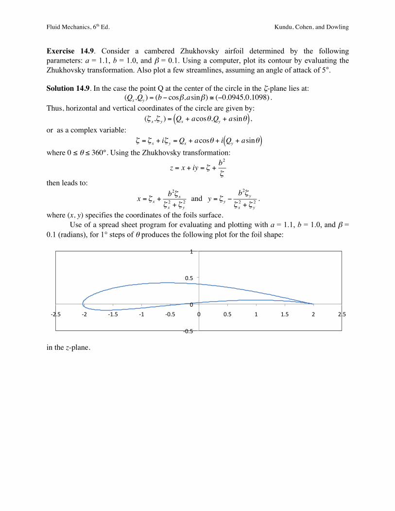
Exercise 14.9. Consider a cambered Zhukhovsky airfoil determined by the following parameters: a = 1.1, b = 1.0, and β = 0.1. Using a computer, plot its contour by evaluating the Zhukhovsky transformation. Also plot a few streamlines, assuming an angle of attack of 5°. Solution 14.9. In the case the point Q at the center of the circle in the ζ-plane lies at:

€

(Qx,Qy ) = (b − cosβ,asinβ) ≅ (−0.0945,0.1098) . Thus, horizontal and vertical coordinates of the circle are given by:

€

(ζ x,ζ y ) = Qx + acosθ,Qy + asinθ( ), or as a complex variable:

€

ζ = ζ x + iζ y =Qx + acosθ + i Qy + asinθ( ) where 0 ≤ θ ≤ 360°. Using the Zhukhovsky transformation:

€

z = x + iy = ζ +b2

ζ

then leads to:

€

x = ζ x +b2ζ x

ζ x2 + ζ y

2 and

€

y = ζ y −b2ζ y

ζ x2 + ζ y

2 .

where (x, y) specifies the coordinates of the foils surface. Use of a spread sheet program for evaluating and plotting with a = 1.1, b = 1.0, and β = 0.1 (radians), for 1° steps of θ produces the following plot for the foil shape:

in the z-plane.

!"#$%

"%

"#$%

&%

!'#$% !'% !&#$% !&% !"#$% "% "#$% &% &#$% '% '#$%


Exercise 14.10. A thin Zhukhovsky airfoil has a lift coefficient of 0.3 at zero incidence. What is the lift coefficient at 5° incidence? Solution 14.10. From (14.12), the lift coefficient of a Zhukhovsky airfoil is:

€

CL = 2π (α + β) . If CL = 0.3 when α = 0, then β = 0.3/2π. Therefore when α = 5°,

€

CL = 2π 5°180°

π +0.32π

#

$ %

&

' ( = 0.848 .


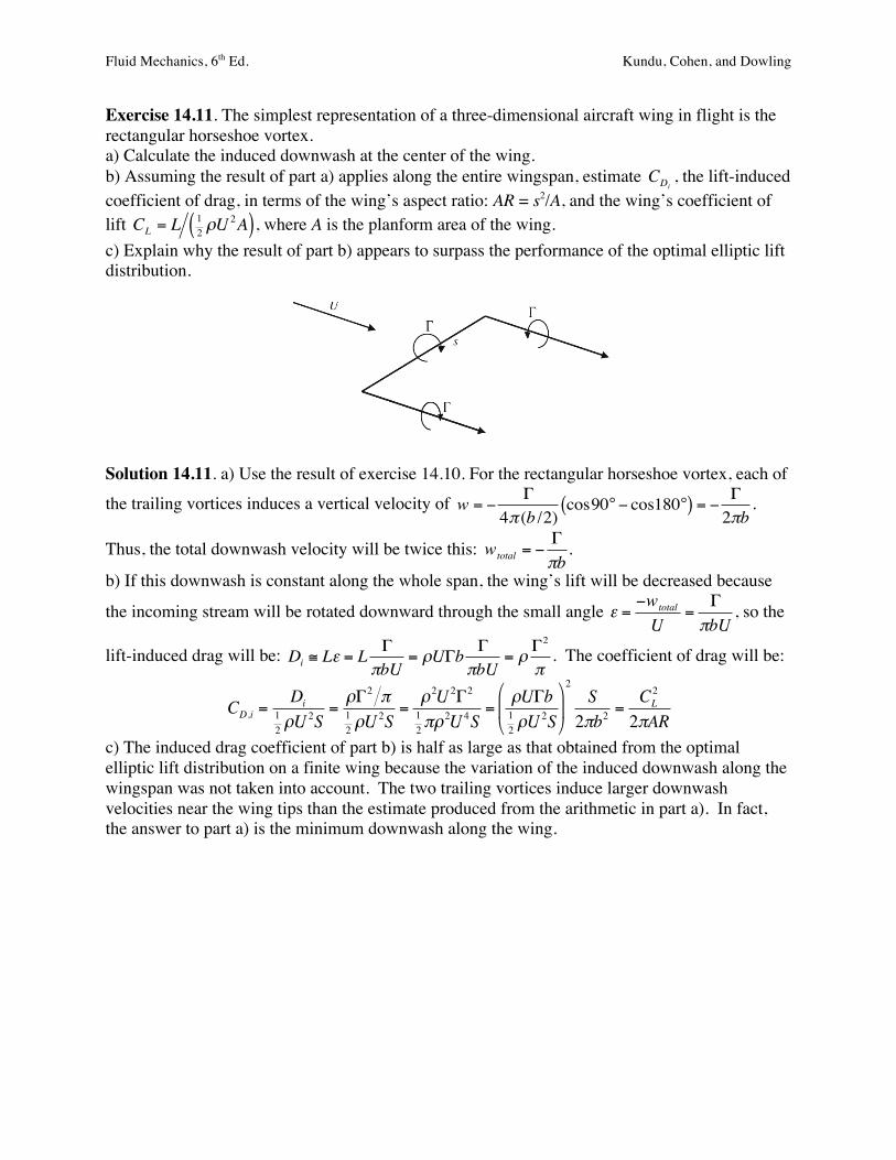
Exercise 14.11. The simplest representation of a three-dimensional aircraft wing in flight is the rectangular horseshoe vortex. a) Calculate the induced downwash at the center of the wing. b) Assuming the result of part a) applies along the entire wingspan, estimate

€

CDi, the lift-induced

coefficient of drag, in terms of the wing’s aspect ratio: AR = s2/A, and the wing’s coefficient of lift

€

CL = L 12 ρU

2A( ), where A is the planform area of the wing. c) Explain why the result of part b) appears to surpass the performance of the optimal elliptic lift distribution.

Solution 14.11. a) Use the result of exercise 14.10. For the rectangular horseshoe vortex, each of

the trailing vortices induces a vertical velocity of

€

w = −Γ

4π (b /2)cos90°− cos180°( ) = −

Γ2πb

.

Thus, the total downwash velocity will be twice this:

€

wtotal = −Γπb

.

b) If this downwash is constant along the whole span, the wing’s lift will be decreased because

the incoming stream will be rotated downward through the small angle

€

ε =−wtotal

U=

ΓπbU

, so the

lift-induced drag will be:

€

Di ≅ Lε = L ΓπbU

= ρUΓb ΓπbU

= ρΓ2

π. The coefficient of drag will be:

€

CD,i =Di

12 ρU

2S=ρΓ2 π12 ρU

2S=

ρ2U 2Γ212 πρ

2U 4S=

ρUΓb12 ρU

2S

%

& '

(

) *

2S

2πb2=

CL2

2πAR

c) The induced drag coefficient of part b) is half as large as that obtained from the optimal elliptic lift distribution on a finite wing because the variation of the induced downwash along the wingspan was not taken into account. The two trailing vortices induce larger downwash velocities near the wing tips than the estimate produced from the arithmetic in part a). In fact, the answer to part a) is the minimum downwash along the wing.


Exercise 14.12. The circulation across the span of a wing follows the parabolic law

€

Γ = Γ0 1− 2y s( )2( ) . Calculate the induced velocity w at midspan, and compare the value with that obtained when the distribution is elliptic.

Solution 14.12. From

€

Γ = Γ0 1− 2y s( )2( ) , determine

€

dΓdy

= −8Γ0 y s2 . Then, from (14.13)

€

w(y1) =14π

dΓdy

dyy1 − y−s 2

+s 2

∫ =8Γ04πs2

ydyy − y1−s 2

+s 2

∫ =2Γ0πs2

y + y1 ln y − y1( )[ ]−s 2

+s 2=2Γ0πs2

s+ y1 lny1 − s 2y1 + s 2&

' (

)

* +

,

- .

/

0 1 .

This downwash distribution varies along the span and at midspan, y1 = 0, it is:

€

w(0) =2Γ0πs

.

In contrast, the constant downwash for an elliptic distribution,

€

Γ 2s, is lower.


Exercise 14.13. An untwisted elliptic wing of 20-m span supports a weight of 80,000 N in a level flight at 300 km/hr. Assuming sea level conditions, find (i) the induced drag and (ii) the circulation around sections halfway along each wing. Solution 14.13. (i) An untwisted wing with an elliptic area is expected to have an elliptic circulation distribution. The induce drag in this case is given by (14.25):

€

Di =2L2

πρU 2s2=

2(8 ×104N)2

π (1.2kgm−3)(83.3ms−1)2(20m)2=1.22kN ,

where 300 km/hr has been converted to 83.3 m/s. (ii) Also from (14.25), the maximum circulation Γ1 is

€

Di =π8ρΓ1

2 and this implies

€

Γ1 = 8Di ρπ = 8(1.22 ×103N) π (1.2kgm−3) = 50.9m2s−1.

Halfway along each wing:

€

Γ(±s /4) = Γ1 1−2(±s /4)

s$

% &

'

( ) 2$

% & &

'

( ) )

1 2

= 50.9m2

s1− 1

2$

% & '

( ) 2$

% & &

'

( ) )

1 2

= 44.1m2

s.


Exercise 14.14 . A wing with a rectangular planform (span = s, chord = c) and uniform airfoil section without camber is twisted so that its geometrical angle, αw, decreases from αr at the root (y = 0) to zero at the wing tips (y = ± s/2) according to the distribution:

€

αw (y) =α r 1− 2y s( )2 . a) At what global angle of attack, αt, should this wing be flown so that it has an elliptical lift distribution? The local angle of attack at any location along the span will be αt + αw. Assume the two-dimensional lift curve slope of the foil section is K. b) Evaluate the lift and the lift-induced drag forces on the wing at the angle of attack determined in part a) when: αr = 2°, K = 5.8 rad.–1, c = 1.5 m, s = 9 m, the air density is 1 kg/m3, and the airspeed is 150 m/s Solution 14.14. a) For an elliptical lift distribution without camber (β = 0), only the first two terms of the finite wing lifting line equation (14.20) are needed:

€

K2Ucα = 1+

cKn4ssinγ

$

% &

'

( )

n=1

∞

∑ Γn sin(nγ) .

The first two terms of this non-traditional Fourier series “solution” are obtained by matching the left side of the equation to the right side evaluated at n = 1.

€

K2Ucα = 1+

cK4ssinγ

$

% &

'

( ) Γ1 sin(γ) = Γ1 sin(γ) +

cK4s

Γ1

For the wing twist specified in the problem statement,

€

α =α t +αw =α t +α r 1− 2y s( )2 . Now, switch to the angle coordinate,

€

y = − s 2( )cosγ , of the lifting line equation so that

€

α =α t +α r sinγ , and plug this into the last equation:

€

K2Uc α t +α r sin(γ)( ) = Γ1 sin(γ) +

cK4s

Γ1.

Require equality of the constant and sinγ terms on both sides of the equation:

€

K2Ucα t = +

cK4s

Γ1 , and

€

K2Ucα r = Γ1.

Eliminate Γ1 and solve for αt;

€

α t = Kcα r (4s). Note that this angle is positive so the wing must be pitched slightly upward. For the parameters given in part b) the value of αt is 0.48°.

b) The lift will be:

€

L =πs4ρUΓ1 =

πsc8ρU 2Kα r , so

€

L =π (9m)(1.5m)

8(1kg /m3)(150m /s)2(5.8 /rad.)(2° ⋅ π /180°)= 24,150 N

The lift-induced drag will be:

€

Di =π8ρΓ1

2 =π32

ρU 2c 2K 2α r2 , so

€

Di =π32(1kg /m3) (150m /s)(1.5m)(5.8 /rad.)(2° ⋅ π /180°)[ ]2 = 204 N

At a flight speed of 150 m/s, overcoming this drag force requires ~30 kW (40 hp).


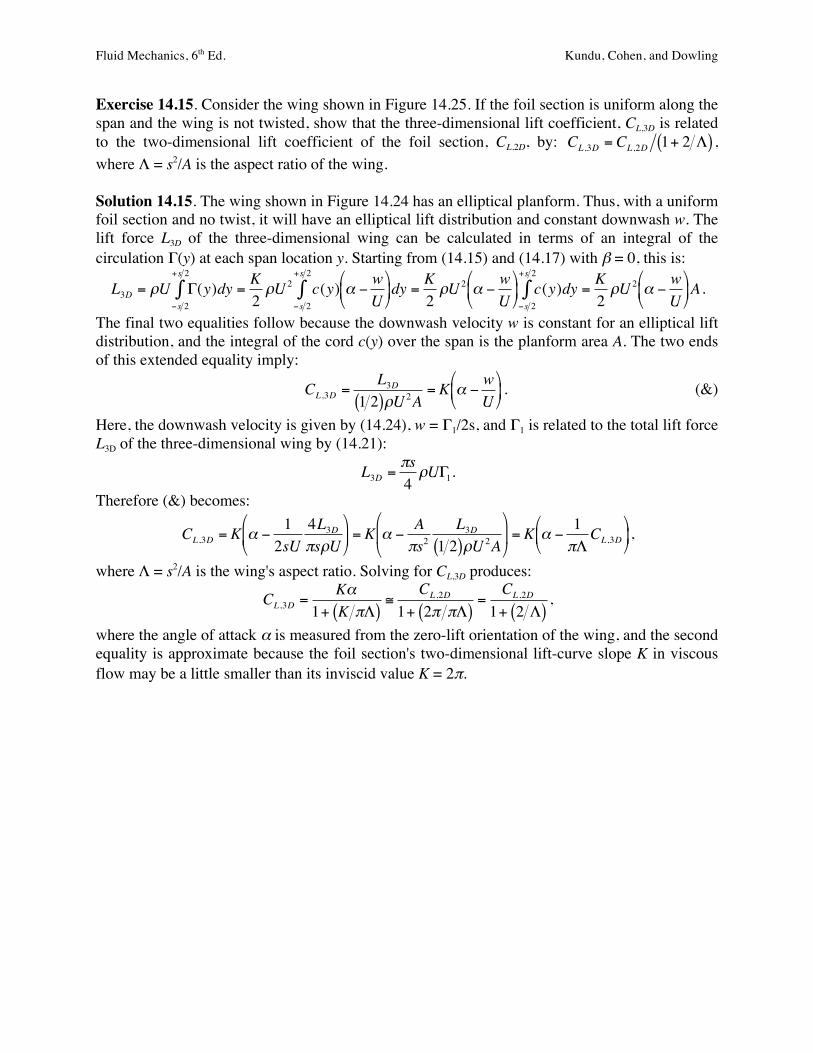
Exercise 14.15. Consider the wing shown in Figure 14.25. If the foil section is uniform along the span and the wing is not twisted, show that the three-dimensional lift coefficient, CL,3D is related to the two-dimensional lift coefficient of the foil section, CL,2D, by:

€

CL,3D = CL,2D 1+ 2 Λ( ) , where Λ = s2/A is the aspect ratio of the wing. Solution 14.15. The wing shown in Figure 14.24 has an elliptical planform. Thus, with a uniform foil section and no twist, it will have an elliptical lift distribution and constant downwash w. The lift force L3D of the three-dimensional wing can be calculated in terms of an integral of the circulation Γ(y) at each span location y. Starting from (14.15) and (14.17) with β = 0, this is:

€

L3D = ρU Γ(y)dy−s 2

+s 2

∫ =K2ρU 2 c(y) α − w

U'

( )

*

+ , dy

−s 2

+s 2

∫ =K2ρU 2 α −

wU

'

( )

*

+ , c(y)dy−s 2

+s 2

∫ =K2ρU 2 α −

wU

'

( )

*

+ , A .

The final two equalities follow because the downwash velocity w is constant for an elliptical lift distribution, and the integral of the cord c(y) over the span is the planform area A. The two ends of this extended equality imply:

€

CL,3D =L3D

1 2( )ρU 2A= K α −

wU

%

& '

(

) * . (&)

Here, the downwash velocity is given by (14.24), w = Γ1/2s, and Γ1 is related to the total lift force L3D of the three-dimensional wing by (14.21):

€

L3D =πs4ρUΓ1.

Therefore (&) becomes:

€

CL,3D = K α −12sU

4L3DπsρU

&

' (

)

* + = K α −

Aπs2

L3D1 2( )ρU 2A

&

' (

)

* + = K α −

1πΛ

CL,3D&

' (

)

* + ,

where Λ = s2/A is the wing's aspect ratio. Solving for CL,3D produces:

€

CL,3D =Kα

1+ K πΛ( )≅

CL ,2D

1+ 2π πΛ( )=

CL ,2D

1+ 2 Λ( ),

where the angle of attack α is measured from the zero-lift orientation of the wing, and the second equality is approximate because the foil section's two-dimensional lift-curve slope K in viscous flow may be a little smaller than its inviscid value K = 2π.


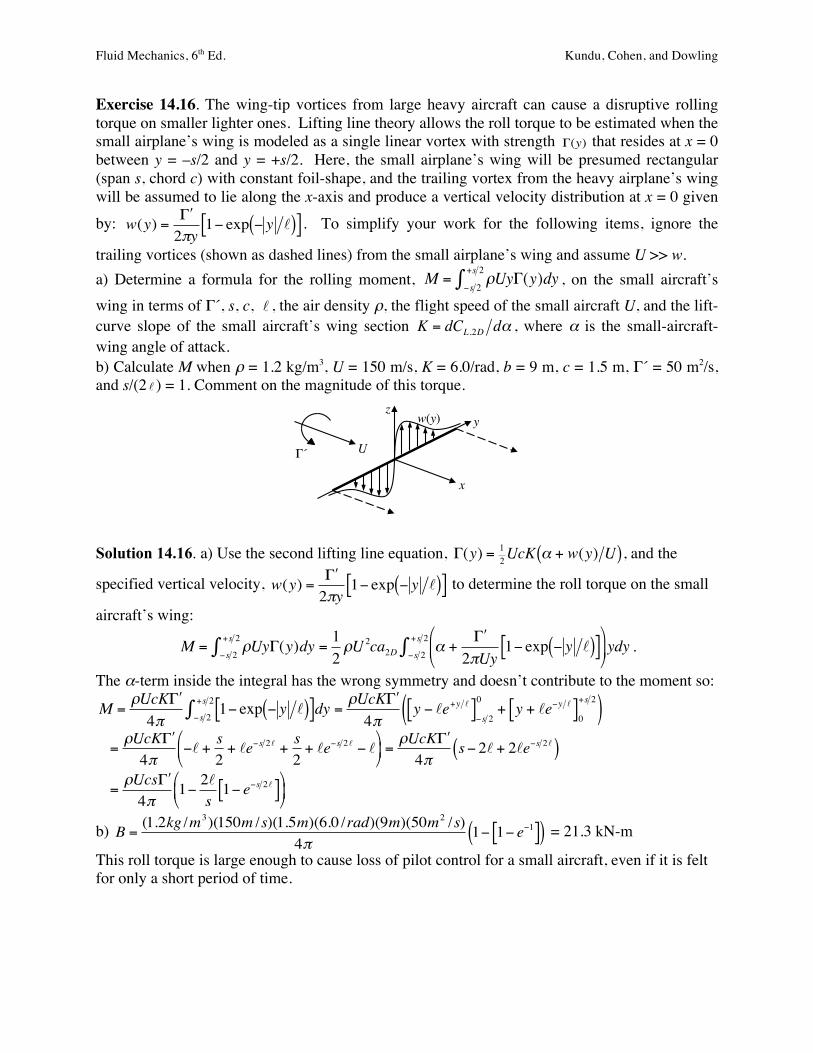
Exercise 14.16. The wing-tip vortices from large heavy aircraft can cause a disruptive rolling torque on smaller lighter ones. Lifting line theory allows the roll torque to be estimated when the small airplane’s wing is modeled as a single linear vortex with strength

€

Γ(y) that resides at x = 0 between y = –s/2 and y = +s/2. Here, the small airplane’s wing will be presumed rectangular (span s, chord c) with constant foil-shape, and the trailing vortex from the heavy airplane’s wing will be assumed to lie along the x-axis and produce a vertical velocity distribution at x = 0 given by:

€

w(y) =" Γ

2πy1− exp − y ( )[ ] . To simplify your work for the following items, ignore the

trailing vortices (shown as dashed lines) from the small airplane’s wing and assume U >> w. a) Determine a formula for the rolling moment,

€

M = ρUyΓ(y)dy−s 2

+s 2∫ , on the small aircraft’s

wing in terms of Γ´, s, c, , the air density ρ, the flight speed of the small aircraft U, and the lift-curve slope of the small aircraft’s wing section

€

K = dCL,2D dα , where α is the small-aircraft-wing angle of attack. b) Calculate M when ρ = 1.2 kg/m3, U = 150 m/s, K = 6.0/rad, b = 9 m, c = 1.5 m, Γ´ = 50 m2/s, and s/(2

€

) = 1. Comment on the magnitude of this torque.

Solution 14.16. a) Use the second lifting line equation,

€

Γ(y) = 12UcK α + w(y) U( ), and the

specified vertical velocity,

€

w(y) =" Γ

2πy1− exp − y ( )[ ] to determine the roll torque on the small

aircraft’s wing:

€

M = ρUyΓ(y)dy−s 2

+s 2∫ =

12ρU 2ca2D α +

' Γ 2πUy

1− exp − y ( )[ ])

* +

,

- . ydy−s 2

+s 2∫ .

The α-term inside the integral has the wrong symmetry and doesn’t contribute to the moment so:

€

M =ρUcK # Γ 4π

1− exp − y ( )[ ]dy−s 2

+s 2∫ =

ρUcK # Γ 4π

y − e+y [ ]−s 2

0+ y + e−y [ ]0

+s 2( )

€

=ρUcK # Γ 4π

− +s2

+ e−s 2 +s2

+ e−s 2 − '

( )

*

+ , =

ρUcK # Γ 4π

s− 2 + 2e−s 2( )

€

=ρUcs # Γ 4π

1− 2s1− e−s 2[ ]

'

( )

*

+ ,

b)

€

B =(1.2kg /m3)(150m /s)(1.5m)(6.0 /rad)(9m)(50m2 /s)

4π1− 1− e−1[ ]( ) = 21.3 kN-m

This roll torque is large enough to cause loss of pilot control for a small aircraft, even if it is felt for only a short period of time.

€

w(y)! y!

x!

z!

U!´!


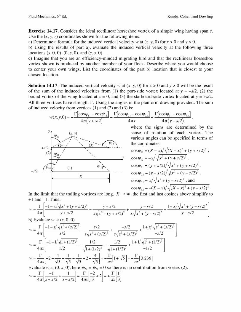
Exercise 14.17. Consider the ideal rectilinear horseshoe vortex of a simple wing having span s. Use the (x, y, z) coordinates shown for the following items. a) Determine a formula for the induced vertical velocity w at (x, y, 0) for x > 0 and y > 0. b) Using the results of part a), evaluate the induced vertical velocity at the following three locations (s, 0, 0), (0, s, 0), and (s, s, 0) c) Imagine that you are an efficiency-minded migrating bird and that the rectilinear horseshoe vortex shown is produced by another member of your flock. Describe where you would choose to center your own wings. List the coordinates of the part b) location that is closest to your chosen location. Solution 14.17. The induced vertical velocity w at (x, y, 0) for x > 0 and y > 0 will be the result of the sum of the induced velocities from (1) the port-side vortex located at y = –s/2, (2) the bound vortex of the wing located at x = 0, and (3) the starboard-side vortex located at y = +s/2. All three vortices have strength Γ. Using the angles in the planform drawing provided. The sum of induced velocity from vortices (1) and (2) and (3) is:

€

w(x,y,0) = −Γ cosψ11 − cosψ11[ ]4π y + s 2( )

−Γ cosψ21 − cosψ22[ ]

4πx+Γ cosψ31 − cosψ32[ ]

4π y − s 2( ),

where the signs are determined by the sense of rotation of each vortex. The various angles can be specified in terms of the coordinates:

€

cosψ11 = (X − x) (X − x)2 + (y + s /2)2 ,

€

cosψ12 = −x x 2 + (y + s /2)2 ,

€

cosψ21 = (y + s /2) x 2 + (y + s /2)2 ,

€

cosψ22 = (y − s /2) x 2 + (y − s /2)2 ,

€

cosψ31 = x x 2 + (y − s /2)2 , and

€

cosψ32 = −(X − x) (X − x)2 + (y − s /2)2 . In the limit that the trailing vortices are long,

€

X →∞ , the first and last cosines above simplify to +1 and –1. Thus,

€

w =Γ4π

−1− x x 2 + (y + s /2)2

y + s /2−

y + s /2x x 2 + (y + s /2)2

+y − s /2

x x 2 + (y − s /2)2+1+ x x 2 + (y − s /2)2

y − s /2

%

& ' '

(

) * *

b) Evaluate w at (s, 0, 0)

€

w =Γ4π

−1− s s2 + (s /2)2

s /2−

s /2s s2 + (s /2)2

+−s /2

s s2 + (s /2)2+1+ s s2 + (s /2)2

−s /2

%

& ' '

(

) * *

€

w =Γ4πs

−1−1 1+ (1/2)2

1/2−

1/21+ (1/2)2

−1/2

1+ (1/2)2+1+1 12 + (1/2)2

−1/2

%

& ' '

(

) * *

€

w =Γ4πs

−2 − 45−15−15− 2 − 4

5%

& ' (

) * = −

Γπs1+ 5[ ] = −

Γπs

3.236[ ]

Evaluate w at (0, s, 0); here ψ22 = ψ21 = 0 so there is no contribution from vortex (2).

€

w =Γ4π

−1s+ s /2

+1

s− s /2%

& ' (

) * =

Γ4πs

−23

+ 2%

& ' (

) * = +

Γπs

13%

& ' (

) *

x!

y!

!11!!12!

!21!

!22!

!31!

!32!

(x, y)!

+s/2!

–s/2!

X!

(2)!

(1)!

(3)!


Evaluate w at (s, s, 0)

€

w =Γ4π

−1− s s2 + (3s /2)2

3s /2−

s+ s /2s s2 + (3s /2)2

+s /2

s s2 + (s /2)2+1+ s s2 + (s /2)2

s /2

%

& ' '

(

) * *

€

w =Γ4πs

−1−1 1+ (3/2)2

3/2−

3/21+ (3/2)2

+1/2

1+ (1/2)2+1+1 1+ (1/2)2

1/2

%

& ' '

(

) * *

€

w =Γ4πs

−23−

43 13

−313

+15

+ 2 +45

%

& ' (

) * =Γπs

13

+54−1312

%

& '

(

) * = +

Γπs1.151[ ]

c) An efficiency minded bird would like to place its wings in a region of upward induced velocity so that its lift-induced drag is minimized by a beneficial interaction with the vortex system of a companion migrating bird. From the results of part b), the rectilinear horseshoe vortex does produce upward induced velocities for (0, s, 0), and (s, s, 0), but the magnitude is greater for (s, s, 0). Thus, the coordinate location (s, s, 0) is the preferred one, and this choice is verified by observations of real migrating birds that fly in Λ-shaped formations.


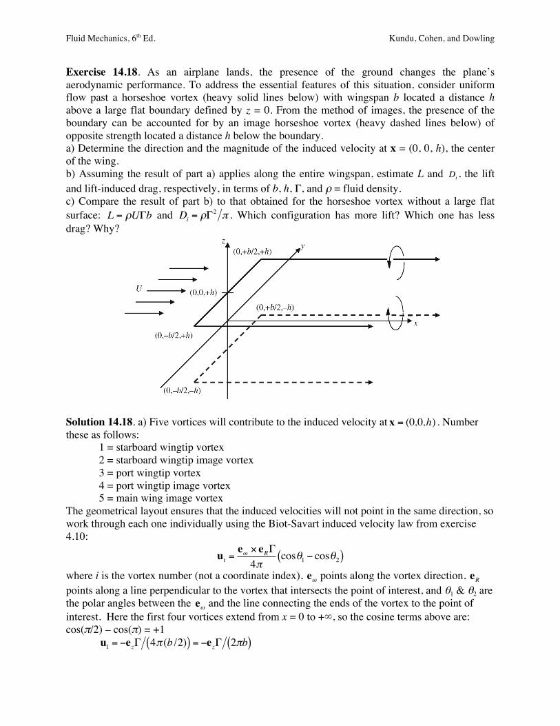
Exercise 14.18. As an airplane lands, the presence of the ground changes the plane’s aerodynamic performance. To address the essential features of this situation, consider uniform flow past a horseshoe vortex (heavy solid lines below) with wingspan b located a distance h above a large flat boundary defined by z = 0. From the method of images, the presence of the boundary can be accounted for by an image horseshoe vortex (heavy dashed lines below) of opposite strength located a distance h below the boundary. a) Determine the direction and the magnitude of the induced velocity at x = (0, 0, h), the center of the wing. b) Assuming the result of part a) applies along the entire wingspan, estimate L and

€

Di , the lift and lift-induced drag, respectively, in terms of b, h, Γ, and ρ = fluid density. c) Compare the result of part b) to that obtained for the horseshoe vortex without a large flat surface:

€

L = ρUΓb and

€

Di = ρΓ2 π . Which configuration has more lift? Which one has less drag? Why?

Solution 14.18. a) Five vortices will contribute to the induced velocity at

€

x = (0,0,h) . Number these as follows: 1 = starboard wingtip vortex 2 = starboard wingtip image vortex 3 = port wingtip vortex 4 = port wingtip image vortex 5 = main wing image vortex The geometrical layout ensures that the induced velocities will not point in the same direction, so work through each one individually using the Biot-Savart induced velocity law from exercise 4.10:

€

ui =eω × eRΓ4π

cosθ1 − cosθ2( )

where i is the vortex number (not a coordinate index),

€

eω points along the vortex direction,

€

eR points along a line perpendicular to the vortex that intersects the point of interest, and θ1 & θ2 are the polar angles between the

€

eω and the line connecting the ends of the vortex to the point of interest. Here the first four vortices extend from x = 0 to +∞, so the cosine terms above are: cos(π/2) – cos(π) = +1

€

u1 = −ezΓ 4π (b /2)( ) = −ezΓ 2πb( )


€

u2 =Γ

4π (b /2)2 + 4h2ez

b /2(b /2)2 + 4h2

+ ey2h

(b /2)2 + 4h2$

% & &

'

( ) )

€

u3 = −ezΓ 4π (b /2)( ) = −ezΓ 2πb( )

€

u4 =Γ

4π (b /2)2 + 4h2ez

b /2(b /2)2 + 4h2

− ey2h

(b /2)2 + 4h2%

& ' '

(

) * *

Here the extra factor in [,] brackets for the second and fourth vortex is merely a unit vector rotated to the induced velocity direction. The fifth, vortex induces a velocity that opposes the on-coming free stream and its angular extent is different from the four other vortices.

€

u5 =−Γex4π (2h)

b /2(b /2)2 + 4h2

−−b /2

(b /2)2 + 4h2%

& ' '

(

) * *

=−Γex2π (2h)

b /2(b /2)2 + 4h2

The sum of these five terms is:

€

utotal = −Γezπb

+Γ

2π (b /2)2 + 4h2ez

b /2(b /2)2 + 4h2

%

& ' '

(

) * * −

Γex2π (2h)

b /2(b /2)2 + 4h2

€

utotal = −Γπb

4h2

(b /2)2 + 4h2% & '

( ) * ez −

Γ4πh

b /2(b /2)2 + 4h2

ex = −uzez − uxex

b) The lift force will be:

€

L = ρ U − wx( )Γb , and the induced drag force will be:

€

Di = Lε = ρ U − wx( )Γbwz

U − wx

= ρΓbwz = ρΓ2

π4h2

(b /2)2 + 4h2' ( )

* + ,

Note, that as h/b → 0, the induced drag disappears. c) For constant speed flight close to the ground surface, there is less lift and less drag for a fixed value of Γ. The lowering of the lift occurs because the induced velocity from the main wing’s image vortex slows the on-coming stream at the location of the real wing. The induced drag is lower because the image tip vortices produce upwash that partially counter acts the downwash from the actual wingtip vortices. For actual aircraft, there are two effects that more than offset the apparent reduction in lift found in part b) and mentioned here. (i) Wing circulation Γ increases as the aircraft approaches the ground because the downwash decreases, and less downwash means an increase in the wing’s angle of attack. (ii) With a constant engine-throttle setting, the loss of induced drag as h/b → 0 causes the aircraft to mildly accelerate, thereby increasing U. The aircraft’s passengers may even feel this mild acceleration, and it may lead to a steady-state speed that prevents the aircraft from descending further and touching down. When this happens the aircraft is said to be flying with or in ground effect. Once the aircraft is low enough for ground effect to be apparent, the pilot must typically reduce the wing's CL by using its spoilers or by lowering the engine throttle setting in a controlled fashion to achieve a safe smooth landing. Observant airline passengers will notice that commercial airliners sometimes fly at very low altitudes over the landing runway for an unexpectedly long period of time before touching down. This apparent delay in touching down is merely the time necessary for pilot to adjust the aircraft's trim to continue its decent while flying in ground effect. [Spoilers are flaps on the top of the wing that spoil the airflow on the suction side of the wing; they are used to increase form drag and reduce lift in a controlled manner.]


Exercise 14.19. Before modifications, an ordinary commercial airliner with wingspan s = 30 m generates two tip vortices of equal and opposite circulation having Rankine velocity profiles (see (3.28)) and a core size σo = 0.5 m for test-flight conditions. The addition of wing-tip treatments (sometimes known as winglets) to both of the aircraft's wing tips doubles the tip vortex core size at the test condition. If the aircraft's weight is negligibly affected by the change, has the lift-induced drag of the aircraft been increased or decreased? Justify your answer. Estimate the percentage change in the induced drag. Solution 14.19. For the conditions stated, the lift-induced drag of the aircraft has decreased by the addition of winglets. This contention is supported by an approximate analysis of the kinetic energy of the vortex flow behind the aircraft. In an unbounded nominally-quiescent fluid medium, an increase in length dl of a single semi-infinite line vortex increases the kinetic energy of the fluid by, dKE, where:

€

dKE =12ρ uθ

22πrdr0

∞∫[ ]dl .

A Rankine vortex is defined by:

€

uθ (r) =Γ 2πσ 2( )r for r ≤σΓ 2πr for r >σ

' ( )

* + ,

where σ is the core size, and r is the distance perpendicular to the vortex axis. Thus, the kinetic energy increment for Rankine vortex is:

€

dKE =12ρ

Γ2πσ 2

&

' (

)

* + 2

0

σ

∫ r22πrdr + limR→∞

Γ2πr&

' (

)

* + 2

σ

R

∫ 2πrdr/

0 1

2

3 4 dl .

The upper limit of the second integral is problematic for a single vortex. However, the airliner will have two wing-tip vortices of equal and opposite sign so evaluation of the limit is not necessary at this point. Performing the two integrations yields:

€

dKE =12ρΓ2

2π1σ 4 r3

0

σ

∫ dr + limR→∞

1rσ

R

∫ dr)

* +

,

- . dl = ρ

Γ2

4π1σ 4

σ 4

4+ lim

R→∞ln r( )σ

R)

* +

,

- . dl

= ρΓ2

4π14

+ limR→∞

lnR( ) − lnσ)

* + ,

- . dl

.

Use the final part of this equality, divide by the time increment dt, and recognize dl/dt = U = the aircraft's velocity, to find:

€

dKEdt

= ρΓ2U4π

14

+ limR→∞

lnR( ) − lnσ)

* + ,

- . .

For an aircraft that produces two counter rotating tip vortices, we can write the following approximate equation

€

dKEdt

≅ 2ρ Γ2U4π

14

+ lnRc − lnσ(

) * +

, - ≅UDi

where Rc is the distance perpendicular to the aircraft's flight path that is large enough for the induced flow from the aircraft's tip vortices to have effectively cancelled out. The final equality here follows because the power necessary to overcome the aircraft's induced drag is that necessary to produce the aircraft's tip-vortex velocity field.


Thus, for comparable flight speed, air density, and aircraft weight, an estimate of the induced drag ratio can be obtained from:

€

Di[ ]modifiedDi[ ]original

=

14

+ lnRc − lnσ$

% & '

( ) modified14

+ lnRc − lnσ$

% & '

( ) original

≈0.25 + ln(90) − ln(1)0.25 + ln(90) − ln(0.5)

=4.755.44

= 0.87 ,

where Rc has been estimated as three times the wing-span of 30 m. Thus, a ~10% (or more) reduction in the induced drag is estimated for a doubling of the tip-vortex core radius from 0.5 m to 1.0 m.


Exercise 14.20. Determine a formula for the range, R, of a long-haul jet-engine aircraft in steady level flight at speed U in terms of: MF = the initial mass of usable fuel; MA = the mass of the airframe, crew, passengers, cargo, and reserve fuel; CL/CD = the aircraft's lift-to-drag ratio; g = the acceleration of gravity; and η = the aircraft's propulsion system thrust-specific fuel consumption (with units of time/length) defined by: dMF/dt = –ηD, where D = the aircraft's aerodynamic drag. For simplicity, assume that U, the ratio CL/CD, and η are constants. [Hints. If M(t) is the instantaneous mass of the flying aircraft, then L = Lift = Mg, M = MF + MA, and dM/dt = dMF/dt. The final formula is known as the Breguet range equation.] Solution 14.20. For steady level flight, an aircraft's engine thrust T will equal its drag D. Thus, the beginning equation is:

dMdt

=dM f

dt= −ηD .

Use the two ends of this extended equality, and divide on the left by M and on the right by L/g. This leads to:

1MdMdt

= −ηD gL= −

1CL CD

gη .

Separate the differential on the left and recognize that Udt = ds = an element of path length along the flight:

1MMF+MA

MA

∫ dM = −1

CL CD

gηU

U dt0

t

∫ = −1

CL CD

gηU

ds0

R

∫ ,

where t is the time of steady level flight and R is the range of the flight. Perform the integrations to find:

ln MA

MA +MF

!

"#

$

%&= −

1CL CD

gηUR .

Solve for R to reach the final form:

R =U CL CD( )

gηln 1+ MF

MA

!

"#

$

%& .

Interestingly, air density does not explicitly enter this formula. Plus, the apparent proportionality between R and U may be somewhat misleading. The aircraft's lift must balance its weight so higher U must be paired with lower CL, and lower U must be paired with higher CL. Plus, CD tends to increase with increasing CL, too (see Figure 14.28), so maximizing the range of a jet engine aircraft means achieving a high lift-to-drag ratio at high speed.

fluid mechanics kundu cohen 6th edition solutions sm ch (14)

Engineering