flowing material balance with water influx flowing material balance with water influx model. once...

1

Flowing Material Balance with Water Influx Mostafa S. Abdelkhalek, BG Group, Ahmed H. El-Banbi, and Mohamed H. Sayyouh, Cairo University

Abstract

Production data analysis is a viable tool for reservoir characterization and estimation of hydrocarbon in

place and reserves. Several methods are available to analyse production data starting with Arps’ classical

decline curve analysis (DCA) in 1945 all the way to more sophisticated analytical and advanced DCA

techniques.

Most of these methods are applicable only for volumetric reservoirs. In this paper, we present a model

that takes into account the effect of water influx on gas reservoir performance.

We introduced the water influx effect into the flowing material balance concept which enables us to

estimate the reservoir pressure and hydrocarbon in place for water drive reservoirs. The model is based on

coupling the material balance equation for gas reservoirs, aquifer models, and the gas flow equation to

calculate the well’s production rate versus time. The model can also estimate reservoir pressure, hydrocarbon

saturation, water rate, and gas rate with time.

When the model is run in history match mode to match gas and water production, we can estimate

original gas in place, well’s productivity index, and aquifer parameters. The model can also be run in

prediction mode to predict gas and water production at any conditions of bottom-hole flowing pressure (or

surface tubing pressure) and reserves can be calculated.

The model was validated with several simulated cases at variable conditions of rate and pressure. The

model was then used to perform decline curve analysis in several field cases. This technique is fast and

requires minimum input data. The paper will present the application of this technique to analyse production

data of 4 gas wells producing both gas and water.

Introduction

Several methods are available to analyse reservoir performance which can be used to estimate initial

hydrocarbon in place, hydrocarbon production rate, water production rate, hydrocarbon saturation, and

reservoir pressure.

These methods can be classified into 3 categories:

1- Classical material balance

2- Numerical reservoir simulation

3- Dynamic production data analysis

Classical material balance can mainly be used to estimate initial hydrocarbon in place and identify the

reservoir drive mechanism. One of the main inputs for this method is the static reservoir pressure on regular

basis. Static reservoir pressure measurement requires wells’ shut-in and running a pressure gauge in the well

or installation of permanent down-hole pressure gauge (PDHG) and measuring the static pressure when the

well is shut-in for long time. Shut-in production wells for a static pressure measurement is not always

justifiable which might impose a constraint on applying this method.

Numerical reservoir simulation can also be used to analyse reservoir performance, but it requires large

amounts of data and it can be time consuming to build the static and dynamic model. The model has also to

be validated and history-matched against actual production and pressure data which may not be available

sometimes (e.g. case of little or no production history of the field).

Dynamic production data analysis is another approach to analyse and estimate reservoir performance.

There are several methods available for that:

2

a- Arps’ Decline Curve Analysis (DCA)

b- Fetkovich type curve

c- Blasingame type curve.

d- Agarwal-Gardner type curve

e- Flowing material balance

The production data analysis methods started since 1920s when a decline trend was used as a tool for

economic evaluation. Arps in 1945 came up with the classical decline curve analysis (DCA) technique which is

based on pure empirical observation.

Arps DCA can be used to estimate the reserves for declining production well. It cannot be used to estimate

hydrocarbon in place or dynamic performance data; such as, reservoir pressure, gas saturation, water rate,

etc. Arps DCA cannot be used also for what-if scenarios (e.g. production against different bottom-hole flowing

pressure).

In 1970s Fetkovich presented his type curve analysis technique that combines the unsteady state flow

solution and the Arps DCA for the pseudo steady state flow. He used the equations from the pressure

transient analysis to represent the unsteady state flow period and blinded it with Arps’ equations to represent

the pseudo steady state flow period.

In 1980s Blasingame et al. presented another type curve analysis technique that overcomes the limitations

of Fetkovich type curve. Blasingame introduced the idea of material balance time which can be used for

variable rate and variable bottom hole flowing pressure (BHFP) cases. Using the material balance time

eliminates the assumption of production under constant BHFP that was the basis for Fetkovich type curve.

Agarwal and Gardner also presented a method to estimate the initial hydrocarbon in place. They

suggested plotting the dimensionless flow rate versus the dimensionless cumulative production on a

Cartesian scale. The result will be a straight line with the intercept with the X axis giving the initial

hydrocarbon in place.

Flowing material balance is used to estimate the initial hydrocarbon in place without the need to shut the

well in for static reservoir pressure measurement. It uses the BHFP along with the production rate in the

pseudo steady state flow period to estimate the hydrocarbon in place.

Most dynamic production data analysis can only be applied on volumetric reservoirs. In others words, DCA

cannot be applied for water drive reservoirs. This limitation arises because most DCA methods are based on

single fluid flow equation which does not account for water flow inside the reservoir.

Approach

Flowing material balance with water influx is an iterative method which requires making an initial guess of

hydrocarbon in place and then making a number of calculations to estimate reservoir pressure as a function

of time. The initial hydrocarbon in place is then back-calculated and convergence with the assumed one can

be checked.

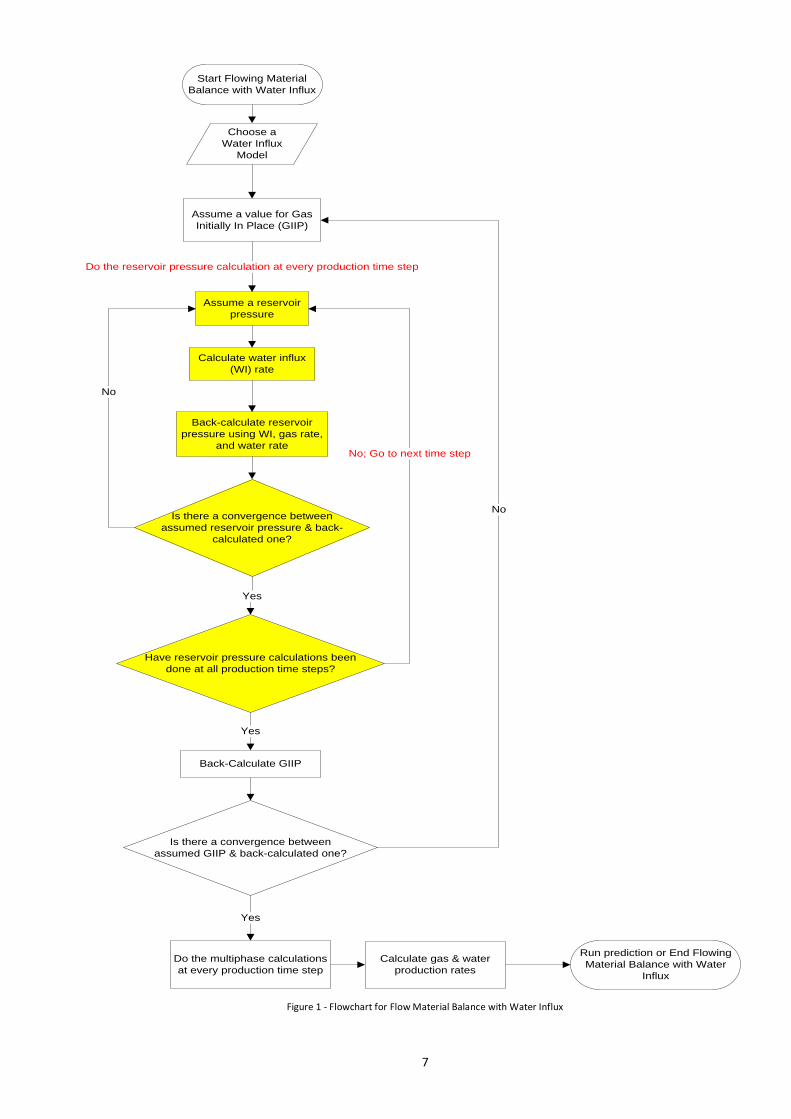
Fig.1 shows a flowchart that describes the iterative process of estimating the initial gas in place from

flowing material balance with water influx model.

Once the initial hydrocarbon in place has been estimated; it can be used along with the estimated

reservoir pressure to history match gas production rate, water production, and gas saturation.

A number of prediction runs can also be obtained at different BHFP scenarios. The outputs of prediction

runs are reservoir pressure, gas rate, water rate, and gas saturation; all as functions of time.

The model has been validated against 3 simulated cases from classical material balance models.

3

Initial Gas in Place

The 4 following equations have been combined together to come up with the equation that represents the flowing material balance with water influx:

1- Conservation of mass 2- Darcy’s law 3- Equation of state 4- Boundary and initial conditions

The final form of the equation of the flowing material balance with water influx has the following shape

………….………… (01)

Eq.1 shows that a plot of the left hand side versus time on a Cartesian scale would yield a straight line. The

slope of the straight line can be used to estimate the initial gas in place.

Input Data

To run the flowing material balance with water influx model, the following data will be needed:

1- Initial reservoir pressure 2- BHFP as function of time 3- Gas and water rate as functions of time 4- PVT data

Model’s Validation

The model was validated with several simulated cases at variable conditions of rate and pressure. The following paragraphs will present the analysis of production data for 3 gas wells producing both gas and water. The validation cases were designed to reveal the capabilities of this paper approach over the available DCA approaches.

Validation Case (1)

Table (1) and (2) show the reservoir and aquifer parameters that were used in a commercial material balance program to generate production and pressure data (MBE).

The model was used with 13 water influx aquifer models and the results obtained with each model were compared to the results obtained from MBE. Table (4) shows the aquifer parameters that can be regressed on to obtain a good solution.

The generated data from MBE was divided into 2 parts; the 1st part was used for history match of our model and the 2nd part was used to run prediction.

Table (3) shows a summary of the estimated GIIP, skin factor, error in reservoir pressure match, error in gas rate match, and error in water rate match compared to the results of the MBE.

The results show that the GIIP error is less than 10% for all the aquifer models except for Schilthuis Steady

State, Hurst Modified Steady State Model, and The Van Everdingen-Hurst Model (Infinite Aquifer) the GIIP

error is greater than 10%.

The error of reservoir pressure, gas saturation, and gas production rate is less than 1.5% for all the aquifer models.

The error of water production rate is less than 20% for 6 aquifer models and less than 30% for 2 more

aquifer models while it is greater than 40% for the rest of the aquifer models.

Figure (2) through figure (6) show a comparison between the results obtained using our model against the

results coming out of the classical material balance equation (MBE). The results have been presented here for

only one aquifer model.

]75.0)([00083.0

**2

])615.5

[(615.5

)]()([

wa

e

giew

sc

sc

sc

wfi

r

rLn

Kht

GBCe

Q

P

ZT

T

PP

PmPmZ

4

Table (5) through table (7) show the input data and the results for the presented aquifer model.

The model has been run in a prediction mode under a certain BHFP secanrio. The prediction run shows

that some aquifer models give a reasonably good preiction match while others not. The results can also be

seen in figure (2) through figure (6).

The following aquifer models give a good results in the prediction run:

1- Pot Aquifer

2- The Van Everdingen-Hurst with finite boundary

3- Fetkovich Radial Model with finite & constant pressure boundary

4- Fetkovich Radial Model with finite & no flow boundary

5- Fetkovich Linear Model with finite & constant pressure boundary

6- Fetkovich Linear Model with finite & no flow boundary

7- Fetkovich Model (Bottom Drive)

The prediction results have been compared to the MBE prediction results. Table (8) shows the error in the

predicted reservoir pressure, gas production rate, water production rate, and gas saturation.

The reservoir pressure error is less than 2% for all aquifer models, the gas rate error is less than 10% for all

aquifer models, and the gas saturation error is less than 6% for all aquifer models.

The water rate error is less than 10% for 8 aquifer models and greater than 10% for the rest of the aquifer

models

Validation Case (2)

Table (9) and (10) show the reservoir and aquifer parameters that have been used in the classical material balance equation (MBE).

The model has been used with 13 water influx aquifer models and the results obtained with each model have been compared to the results obtained from MBE.

The generated data from MBE was divided into 2 parts; the 1st part was used for history match of our model and the 2nd part was used to run prediction.


The results show that the GIIP error is less than 5% for 8 aquifer models and less than 20% for 4 aquifer

models while it is greater than 20% for just 1 aquifer model.

The error of reservoir pressure, gas saturation, and gas production rate is less than 1% for all the aquifer

models.

The error of water production rate is less than 10% for 8 aquifer models and less than 20% for 3 more

aquifer models while it is greater than 20% for just 2 aquifer models.

Figure (7) through figure (11) show a comparison between the results obtained using our model against

the results coming out of the classical material balance equation (MBE). The results have been presented here

for only one aquifer model. Table (12) through table (14) show the input data and the results for the

presented aquifer model.

The model has been run in a prediction mode under a certain BHFP secanrio. The prediction run shows

that some aquifer models give a reasonably good preiction match while others not.

The prediction results have been compared to the MBE prediction results. Table (15) shows the error in

the predicted reservoir pressure, gas production rate, water production rate, and gas saturation.

The reservoir pressure error is less than 1% for all aquifer models, the gas rate error is less than 20% for all

aquifer models, and the gas saturation error is less than 2% for all aquifer models while water rate error is

less than 20% for 10 aquifer models.

5

Validation Case (3)

Table (16) and (17) show the reservoir and aquifer parameters that have been used in the classical material balance equation (MBE).

The model has been used with 11 different water influx aquifer models and the results obtained with each model have been compared to the results obtained from MBE.


The results show that the GIIP error is less than 5% for 6 aquifer models and less than 25% for 2 aquifer

models while it is greater than 25% for 3 aquifer models. The error of reservoir pressure and gas saturation is

less than 1.0% for all the aquifer models. The error of gas production rate and water production rate is less

than 10% for all the aquifer models.


the results coming out of the classical material balance equation (MBE). The results have been presented here

for only one aquifer model. Table (19) through table (21) show the input data and the results for the

presented aquifer model.

This validation case does not have a prediction run due to having a very low gas production rate (less than

5 MMscfd) at the end of the history period.

Field Case

Our model has been used to calculate reserves and predict the performance of real field data from a gas

reservoir under water influx.

The model has been used with 11 different water influx aquifer models and the results obtained with each aquifer model have been compared to the actual field data.

Table (22) shows a summary of the estimated GIIP, skin factor, error in reservoir pressure match, error in gas rate match, and error in water rate match compared to the actual field data.

The error of reservoir pressure, gas rate and water rate is less than 11% for all the aquifer models.


the actual field data.

Conclusions

A new model was developed to estimate the GIIP, reservoir pressure, gas saturation, gas rate, and water rate for gas wells producing from water drive gas reservoirs.

The new model is based on extending the flowing material balance equation to account for water influx.

The model couples material balance for gas reservoirs, IPR or flow equation model, and aquifer models. The model works in both history match and prediction modes.

The model has been validated against 3 simulated cases to show its capabilities. For the 3 cases, the model gave errors as low as 2% for GIIP estimate, 1% for reservoir pressure estimate, and 2% for gas and water production rates.

The model has the capability to be run in prediction mode at variable bottom-hole flowing pressure, hence the ability to test different production scenarios.

Testing this model using a large number of commonly used aquifer models shows the estimated aquifer model may not be unique. However, the prediction under different aquifer models will converge if there is enough historical data.

6

References 1. Ahmed, Tarek and Meehan, Nathan: Advanced Reservoir Management and Engineering, 2nd ed. Oxford, Gulf

Professional Publishing Co., 2012. 2. MATTAR, L. and ANDERSON, Z.: “A Systematic and Comprehensive Methodology for Advanced Analysis of

Production data,” Paper SPE 84472 presented at SPE Annual Meeting and Exhibition, Denver, Colorado, Oct. 5-8, 2003.

3. Houze, Olivier and Viturat, Didier: Dynamic Data Analysis, Paris, KAPPA, 2011. 4. Craft, B. C. and Hawkins, M. F.: Applied Petroleum Reservoir Engineering, 2

nd ed. New Jersey, Prentice Hall

Inc., 1991. 5. MATTAR, L. and ANDERSON, Z.: “Dynamic Material Balance (Oil or Gas in place without shut ins),” Paper

presented at the Petroleum Society’s 6th Canadian International Petroleum Conference, 56th Annual Technical Meeting, Alberta, Canada, June 7 – 9, 2005.

6. Choudhury, Z. and Gomes, E.: “Material Balance Study of Gas Reservoirs by Flowing Well Method: A Case Study of Bakhrabad Gas Field,” Paper SPE 64456 presented at the SPE Asia Pacific Oil and Gas Conference and Exhibition, Brisbane, Australia, October 16–18, 2000.

7. MATTAR, L. and ANDERSON, Z.: “A Systematic and Comprehensive Methodology for Advanced Analysis of Production data,” Paper SPE 84472 presented at SPE Annual Meeting and Exhibition, Denver, Colorado, Oct. 5-8, 2003.

8. Anderson, M. And Blasingame, T. A.: “Production Data Analysis -Challenges, Pitfalls, Diagnostics,” Paper SPE 102048 presented at the 2006 SPE Annual Technical Conference and Exhibition held in San Antonio, Texas, U.S.A., 24–27 September 2006.

Nomenclature

BHFP = Bottom Hole Flowing Pressure, psia

Bg = Gas formation volume factor, ft3/scf

Ce = Effective compressibility factor, psi-1

DCA = Decline Curve Analysis

G = Gas in place, scf

GIIP = Gas in place, scf

h = Reservoir net thickness, ft

K = Reservoir permeability, md

MBE = Material Balance Equation

m(Pi) = Real-gas pseudo pressure at initial reservoir pressure, psi2/cp

m(Pwf) = Real-gas pseudo pressure at BHFP, psi2/cp

P = Reservoir pressure, psia

Psc = Standard condition pressure, psia

Qsc = Gas flow rate, MMscf/d

r = Radius, ft

re = Drainage radius, ft

rwa = Apparent wellbore radius, ft

T = Reservoir temperature, R

Tsc = Standard condition temperature, R

V = Volume, bbl

Z = Gas compressibility factor

μ = Viscosity, cp

Φ = Porosity

7

Start Flowing Material

Balance with Water Influx

Assume a value for Gas

Initially In Place (GIIP)

Assume a reservoir

pressure

Do the reservoir pressure calculation at every production time step

Calculate water influx

(WI) rate

Back-calculate reservoir

pressure using WI, gas rate,

and water rate

Is there a convergence between

assumed reservoir pressure & back-

calculated one?

No

Back-Calculate GIIP

Is there a convergence between

assumed GIIP & back-calculated one?

No

Do the multiphase calculations

at every production time step

Yes

Calculate gas & water

production rates

Run prediction or End Flowing

Material Balance with Water

Influx

Have reservoir pressure calculations been

done at all production time steps?

Yes

Yes

No; Go to next time step

Choose a

Water Influx

Model

Figure 1 - Flowchart for Flow Material Balance with Water Influx

8

Table 1- Validation Case 1 - Reservoir Parameters for MBE

Table 2- Validation Case 1 - Aquifer Parameters for MBE

Table 3- Validation Case 1 - Results Summary for Validation Case (1)

9

Table 4 Aquifer Regression Parameters

Table 5 Validation Case 1 - Reservoir Parameters for Fetkovich Bottom

Drive Aquifer Model

Table 6 Validation Case 1 - Aquifer Parameters for Fetkovich Bottom Drive

Aquifer Model

Table 7 Validation Case 1 - Results Using Fetkovich Bottom Drive Aquifer

Model

Figure 2- Validation Case 1 - Diagnostic Plot Using Fetkovich Bottom Drive

Aquifer Model

Figure 3- Validation Case 1 - Reservoir Pressure Match Using Fetkovich

Bottom Drive Aquifer Model

Figure 4- Validation Case 1 - Gas Saturation Match Using Fetkovich Bottom

Drive Aquifer Model

Figure 5- Validation Case 1 - Gas Rate Match Using Fetkovich Bottom Drive

Aquifer Model

Figure 6- Validation Case 1 - Water Rate Match Using Fetkovich Bottom Drive Aquifer Model

10

Table 8 - Validation Case 1 – Prediction Results Summary

Table 9 Validation Case 2 - Reservoir Parameters for MBE

Table 10 Validation Case 2 - Aquifer Parameters for MBE

Table 11 - Validation Case 2 - Results Summary for Validation Case (2)

11

Table 12 Validation Case 2 - Reservoir Parameters for Fetkovich Radial

Aquifer Model with Infinite Boundary

Table 13 Validation Case 2 - Aquifer Parameters for Fetkovich Radial


Table 14 Validation Case 2 - Results Using Fetkovich Radial Aquifer Model

with Infinite Boundary

Figure 7- Validation Case 2 - Diagnostic Plot Using Fetkovich Radial Aquifer

Model with Infinite Boundary

Figure 8- Validation Case 2 - Reservoir Pressure Match Using Fetkovich

Radial Aquifer Model with Infinite Boundary

Figure 9- Validation Case 2 - Gas Saturation Match Using Fetkovich Radial


Figure 10- Validation Case 2 - Gas Rate Match Using Fetkovich Radial


Figure 11- Validation Case 2 - Water Rate Match Using Fetkovich Radial


12

Table 15 - Validation Case 2 – Prediction Results Summary

Table 16 Validation Case 3 - Reservoir Parameters for MBE

Table 17 Validation Case 3 - Aquifer Parameters for MBE

Table 18 - Validation Case 3 - Results Summary for Validation Case (3)

13

Table 19- Validation Case 3 - Reservoir Parameters for Pot Aquifer Model

Table 20- Validation Case 3 - Aquifer Parameters for Pot Aquifer Model

Table 21- Validation Case 3 - Results Using Pot Aquifer Model

Figure 12- Validation Case 3 - Diagnostic Plot Using Pot Aquifer Model

Figure 13- Validation Case 3 - Reservoir Pressure Match Using Pot Aquifer

Model

Figure 14- Validation Case 3 - Gas Saturation Match Using Pot Aquifer

Model

Figure 15- Validation Case 3 - Gas Rate Match Using Pot Aquifer Model

Figure 16- Validation Case 3 - Water Rate Match Using Pot Aquifer Model

14

Table 22 - Field Case 1 - Results Summary

Figure 17- Field Case 1 - Diagnostic Plot Using Fetkovich Bottom Drive

Aquifer Model

Figure 18- Field Case 1 - Reservoir Pressure Match Using Fetkovich Bottom

Drive Aquifer Model

Figure 19- Field Case 1 - Gas Rate Match Using Fetkovich Bottom Drive

Aquifer Model

Figure 20- Field Case 1 - Water Rate Match Using Fetkovich Bottom Drive

Aquifer Model

flowing material balance with water influx flowing material balance with water influx model. once...

Documents