fixed versus flexible exchange rates: a panel-var

7/27/2019 Fixed versus Flexible Exchange Rates: A Panel-VAR

http://slidepdf.com/reader/full/fixed-versus-flexible-exchange-rates-a-panel-var 1/21

Fixed versus Flexible Exchange Rates: A Panel-VAR

Analysis∗

Mathias Hoff mannDepartment of Economics

University of Cologne†

13th of January 2003

Abstract

This paper empirically investigates Mundell’s (1961) formalisation that in a small open

economy flexible exchange rates act as a ‘shock absorber’. The role of a world real interest

rate shock in driving output, trade imbalances and real exchange rate fluctuations under

diff erent exchange rate regimes is empirically investigated in a Panel VAR, which utilises

economic theory for identification.

JEL Classification: C33, F31, F41

Keywords: Small Open Economies, Exchange Rate Regimes, Panel VAR

∗This work is part of a research network on ’The Analysis of International Capital Markets: Understanding

Europe’s Role in the Global Economy’, funded by the European Commission under the Research Training Network

Programme (Contract No. HPRN-CT-1999-00067).†Address of Correspondence: Mathias Hoff mann, Department of Economics, University of Cologne -Chair

of International Economics, Albertus-Magnus-Platz, 50931 Cologne, Germany. email: m.hoff [email protected]

koeln.de

1



1 Introduction

An important feature of the global economy is the great variety of exchange rate policies. Since

Bretton Woods, the comparative properties of fixed and flexible exchange rates have been of

concern and interest for many international economists and policy makers.1 The experience of

numerous emerging market economies over the last decade has led to a refreshed discussion of

the question whether to adopt a fixed or flexible exchange rate regime (e.g. Obstfeld, 2002;

Lane, 2002). The general argument in favour of flexible exchange rates follows Mundell’s (1961)

formalisation that they act as a ’shock absorber’ in a small economy.

This paper tests the conventional wisdom that external shocks are less contractionary under

floating exchange rates. Especially in small open developing economies, macroeconomic dynam-

ics are heavily influenced by the outside world. The collapse of international prices for their

exports, demand shortfalls, withdrawal of foreign capital or interest rate fluctuations provide

good examples of exogenous macroeconomic dynamics which aff ect open economies. This study

examines the impact of an external shock on a selected group of small open economies, which

have adopted diff erent exchange rate regimes. A panel vector autoregression (PVAR) approach

will be utilised to test whether economies respond diff erently to such shocks. The PVAR captures

both the stochastic patterns and co-movements of macroeconomic variables and allows to study

dynamics in terms of deviations from the equilibrium across countries. The paper analyses and

compares the adjustment process of home real output, the trade balance and the real exchange

rate by concentrating on world real interest rate shocks.

Despite the prominent role played by exchange rate regimes, there is relatively little empirical

work addressing their properties. Baxter and Stockman (1989) focus on correlations in the data

to analyse the variability of output and inflation over time in an atheoretical approach. Their

finding is that diff erent regimes are able to explain shifts in the data. However, a difficulty with

this approach is that a given set of observations may be compatible with diff erent economic

interpretations. To overcome this problem, Bayoumi and Eichengreen (1994) use a VAR model

to analyse nominal and real shocks under diff erent exchange rate regimes. However, the authors

do not explicitly test for any hypothesis underfi

xed andfl

oating exchange rates. Hoff

maister andRoldos (1997) utilise a PVAR approach to analyse business cycle behaviour in Asian and Latin

American countries. Similar to Bayoumi and Eichengreen, they apply the Blanchard and Quah

(1989) approach to separate nominal and real shocks. Except Broda (2000), who concentrates

on terms of trade shocks, there has not been any PVAR research analysing the eff ects of shocks

1 In a classical paper Helpman (1981) formally compares diff erent exchange rate regimes. He points out that

in the presence of no market distortions and perfect foresight all equilibrium allocations are Pareto efficient.

2



under diff erent exchange rate regimes.

The next section explains the role of the world interest rate in a small open economy. While

section 3 outlines the econometric issues involved, section 4 presents the empirical evidence by

utilising pooled time series data. The dynamic adjustment is illustrated by the impulse response

functions. Section 5 concludes.

2 The World Real Interest Rate

Small open economies provide several channels by which world shocks influence their perfor-

mance. In theory, the world real interest rate is an important mechanism by which foreign

shocks and business cycles are transmitted to small economies. In recent years emerging market

economies have faced large disturbances in international financial markets. The collapse of asset

values in Japan at the onset of the current recession can be seen as one event causing such a dis-

turbance, which represents an external financial shock for developing countries. Changes in the

world real interest rate are therefore shocks to the financial system and aff ect the behaviour of

variables in the economy in a unique way, depending on the domestic conditions. By generating

the intertemporal substitution of households, aff ecting wealth as well as the portfolio allocation,

the world real interest rate has an impact on the ‘real side’ of the economy and alters the alloca-

tion of resources. Thus, the world interest rate provides a useful focus for the analysis, since it

causes significant disturbances to real economic performance.2 In an intertemporal model with

nominal rigidities, e.g. sticky prices, the adjustment mechanism also depends on the adoption

of the exchange rate regime. An unexpected temporary increase in the world real interest rate

implies that current consumption becomes relatively more expensive so that consumers favour

future over current consumption. As a result, consumption falls in the short-run. Under a float-

ing exchange rate regime, the nominal and real exchange rate depreciate and raise the relative

price of foreign traded goods. Under an exchange rate peg the fixed nominal exchange rate limits

the response of the real exchange rate. The relative price change makes home produced goods

relatively cheaper under floats. Moreover, a more pronounced trade balance surplus occurs under

floating exchange rates. Consequently, in the floating exchange rate economy home production

would decline to a lesser extent in case of a world real interest rate shock (Hoff mann, 2002). In

the presence of nominal rigidities the nominal exchange rate allows a faster adjustment process

in floating compared to pegging exchange rate economies since there is no need to wait until

2 However, there are some difficulties in obtaining the world interest rate. Obstfeld and Rogoff (1995, p. 1781)

discuss tests of intertemporal current account models and note that it is not obvious which real interest rate

should be used.

3



imbalances in the goods market reduce domestic prices.3

The empirical analysis of the eff ects of the world real interest rate on the small open econ-

omy’s output, trade balance and real exchange rate requires the consideration of interactions

between world output and the world interest rate. The world interest rate and world output are

presumably not independent; movements in world output aff ect the world interest rate. As a

result, to estimate the eff ect of one, it is also necessary to include the other. 4

3 Econometric Approach: Panel VAR

This section explains the econometric method used to test the hypothesis that floating exchange

rates are superior in insulating an economy against external shocks.

3.1 Data

The econometric model considers a set of variables to recover the pattern of shocks in 42 low,

lower and middle income economies (Table 1) for the sampling period 1973 to 1999. All data,

except the world interest rate and net exports, are measured in logs. To measure the world real

interest rate the method suggested by Barro and Sala-i-Martin (1990) and applied by Bergin and

Sheff rin (2000) is utilised. Short-term nominal interest rates of the G-7 countries are adjusted by

the inflation expectations to calculate the ex-ante real interest rate for each of the G-7 countries.5

To compute an individual average world real interest rate for country i in the sample, weights

based on the trade shares of country i with each of the G-7 countries are used to construct

a modified world real interest rate since loans to developing countries by the G-7 countries are

closely related to their trade flows with such countries. The world real output is measured by the

trade weighted GDP of the countries’ trading partners in constant currency units. To construct

the home real output, the developing countries’ GDP is utilised in constant units.6 Countries’

net exports are measured by the external balance on goods and services as a percentage of GDP

in constant domestic currency units. The countries’ real exchange rate is the ratio of CPI indexes,

3 This is in line with the argument brought forward by Friedman (1953).

4 For example, in times of high world output, demand for investment may be high and so may be the world

interest rate.5 Inflation expectations are forecasts, calculated by a six-quarter autoregression (Bergin, 2001).6 The real output data are measured in domestic currencies to overcome the real exchange rate eff ects, which

would influence the data if they were obtained in US dollar terms. To see this more clearly, consider the following

equality:Y Hi/$

P i/$=

S$/HomeCurrency∗Y Hi

P i/$=

S$/HomeCurrency

P i/$∗ P i ∗

Y HiP i

.

Thus, real output is measured in terms of constant domestic currency units.

4



adjusted by the nominal exchange rate (national currency per dollar).7

3.2 Nonstationarity and Cointegration

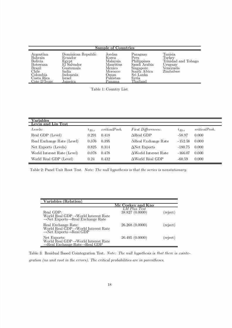
Prior to the statistical analysis the data series are tested for unit roots and cointegration, since a

necessity for calculating means and variances is the data’s stationarity.8 The Levin and Lin Test

(1992) is utilised to test the null hypothesis of nonstationarity. Table 2 presents the test results.

Overall, there is no evidence for the data’s stationarity in levels. However, the data appear to be

stationary in first diff erences (Table 2). Given that the time series properties of the data are not

stationary in levels the null hypothesis that the variables are cointegrated is tested. Mc Coskey

and Kao (1998) derive such a residual based test statistic. Table 3 depicts the results and shows

that there does not exist a long-run relationship between the variables. Hence, the econometric

model is estimated in first diff erences without imposing any cointegration relationship. Given the

time series properties of the data set, Table 4 presents the summary statistics of the data used in

the empirical analysis. It becomes apparent that the real exchange rate appreciates or depreciates

on average more strongly under floats than under pegs during the sample period under both,

the de jure and de facto specification.9 The standard deviation of the real exchange rate is

always higher under floats, which implies that a higher real exchange rate volatility is evident in

floating countries. Table 4 also shows that under pegs average net exports are lower and even

negative when considering the de facto specification. Additionally, fixed exchange rate economies

experience a higher volatility in net exports on average. Interestingly, the statistical analysisdemonstrates that the average growth rate of real GDP is higher under the de jure specification

in countries which adopt a fixed exchange rate. Nevertheless, under both specifications the real

GDP growth rate is more volatile under pegs than under floats.10

3.3 Choice of Exchange Rate Regimes

Following Frankel (1999), nine exchange rate regimes exist, which can be categorised into three

types. Currency unions, currency boards and truly fixed exchange rates can be specified as fixed

exchange rates . Intermediate regimes comprise crawling pegs (adjustable pegs, crawling pegsand basket pegs) and dirty floats (target zone/bands or managed floats). Free floats represent a

7 Short-term nominal interest rates are derived from the International Financial Statistics (International Mon-

etary Fund, 2000). Output data and net exports are obtained from the World Development Indicators (World

Bank, 2001). Data on the real exchange rate are taken from Lane and Milesi-Ferretti (2002) and are re-based so

that a rise in the real exchange rate reflects a depreciation and a fall an appreciation.8 Tests are implemented using the NPT 1.2 in Gauss, provided by Chiang and Kao (2001).9 For a discussion of the two exchange rate specifications please refer to the next section.

10 According to Taylor (1989) flexible exchange rates reduce output volatility by almost one half.

5



pure float regime. For the econometric analysis intermediate regimes are considered under the

floating category.

This paper follows the recent work by Reinhart and Rogoff (2002) and the International

Monetary Fund’s (2000) Annual Report on Exchange Arrangements and Exchange Rate Re-

strictions (AREAER) to classify the exchange rate regimes of the 42 countries of interest. The

AREAER report is based on the publicly stated commitment of the authorities in the countries

in question, known as the de jure analysis. The approach is problematic since it constitutes the

uncertainty of not knowing whether the actual policy in the country is consistent with the com-

mitment stated in the AREAER (e.g. Frankel, 1999; Reinhart and Rogoff , 2002). This problem

can be overcome by basing the classification on the observed behaviour of the exchange rate.

Thus, data on interventions (reserve changes), exchange rate volatility, exchange rate changes or

market-determined parallel exchange rates can be applied. Reinhart and Rogoff

(2002) utilisethe de facto approach, which forms the basis of the following empirical analysis and is compared

to the de jure approach. An overview of the de jure and de facto approaches in the country set

indicates a clear trend towards a floating exchange rate policy. However, diff erences between

the two approaches emerged from the mid 70s to the mid 80s, where a policy towards floating

exchange rate regimes prevailed under the de facto specification. By contrast, under the de jure

specification such a clear trend towards floating exchange rates was not evident.

3.4 Identification of the Econometric Model

Developing countries represent the focal point of attention of the empirical analysis so that the

econometric application is derived from small open economy assumptions. Domestic innovations

do not aff ect external variables, i.e. the world real interest rate, r , and world (foreign) real

output, y Foreign. To be more precise, it is assumed that current and past values of the real

exchange rate, rer , real home output, y Home, and net exports, nx , of a small open economy do

not aff ect r and y Foreign, neither in the short nor in the long-run. However, the data generation

process of home output, the trade balance and the real exchange rate is aff ected by world output

and the world real interest rate, which are determined outside of the system under investigation.

Additionally, the real exchange rate, the trade balance and domestic output are jointly influenced

by movements of one of the three variables.11 The joint eff ects on home output, net exports and

the real exchange rate complicate the identification of structural innovations in a model which

11 For example, changes in the real exchange rate impact on the private sector’s real wealth and expenditure

through its eff ect on domestic prices. The change in domestic absorption leads firms to revise expectations on

future demand and, hence, alters production. This aff ects aggregate supply and, therefore, output and the trade

balance. The latter has an impact on home prices and has feedback eff ects on the real exchange rate.

6



contains all variables. To overcome this problem an exogenous Vector Autoregression (VARX)

model is applied in which world output and the world real interest rate are treated as exogenous

variables. This approach imposes no restrictions on the model.12 The exogeneity of world output

and the world real interest rate enables the tracing of such shocks through the system. 13 The

econometric model takes the following reduced form:

Yi,t = B(L)Yi,t +C0Xi,t +C(L)Xi,t + ui,t. (1)

Yi,t is the 3 x 1 dependent and endogenous variable vector. Yi,t =£∆ log y Home,∆ logRER,∆nx

¤0

comprises real home output, the real exchange rate and net exports. Xi,t =£∆ log y Foreign,∆r

¤0

is a 2 x 1 vector of the exogenous real world output and the world real interest rate. ui,t reflects

the model’s error term. B(L) and C(L) are matrix polynomials in the lag operator.14 To exam-

ine whether the responses of the exogenous shocks are diff erent between regimes, the estimated

model allows to interact B(L), C0 and C(L) with the dummies Dfixi,t and Dfloati,t, which

capture the eff ects of the diff erent exchange rate regimes. Countries that float today might peg

their exchange rate tomorrow, which would consequently lead to a confusion between responses

of floats and pegs. To overcome this potential source of bias, the sample includes only observa-

tions of countries with the same exchange rate regime during four periods.15 From equation (1)

the representation of the exogenous process takes the form

yi,t =

∞

Xs=0

J BsC

x i,t−s +

∞

Xs=0

J Bs

J

0

u i,t−s. (2)

The expression in equation (2) allows the derivation of the impulse response functions for a

given exogenous shock to the system (section 4). To examine whether the findings and responses

to the real shock are robust a sensitivity analysis will be applied. 16 In this context, impulse

responses obtained from the de facto approach are compared with responses under the de jure

specification, given the shock to the world real interest rate.

12 The reduced form model is obtained by the premultiplication of the inverted non-singular instantaneous

eff ects matrix.13 Hoff mann (2002) also considers a shock to world output.

14B(L) =B1L + ... + BsLs and C(L) =C 1L + ... + C pLp.15 This issue was also raised by Broda (2000).16 In Hoff mann (2002) several robustness checks are applied. The sample was split in order to be able to at-

tribute responses to diff erent exchange rate regimes which actually might be associated with other characteristics.

Financial openness and the degree of trade openness are factors which may aff ect the overall results found for the

world real interest rate.

7



4 Empirical Results

The empirical model in section 3.4 is estimated by generalised least square (GLS). 17 It can be

used to compute the dynamic response functions, which study the eff ects of changes in the world

real interest rate on domestic real output of countries as well as their real exchange rate and

net exports. The impulse response functions are accompanied by one standard deviation error

bands.18

4.1 World Real Interest Rate: Fixed versus Flexible Exchange Rates

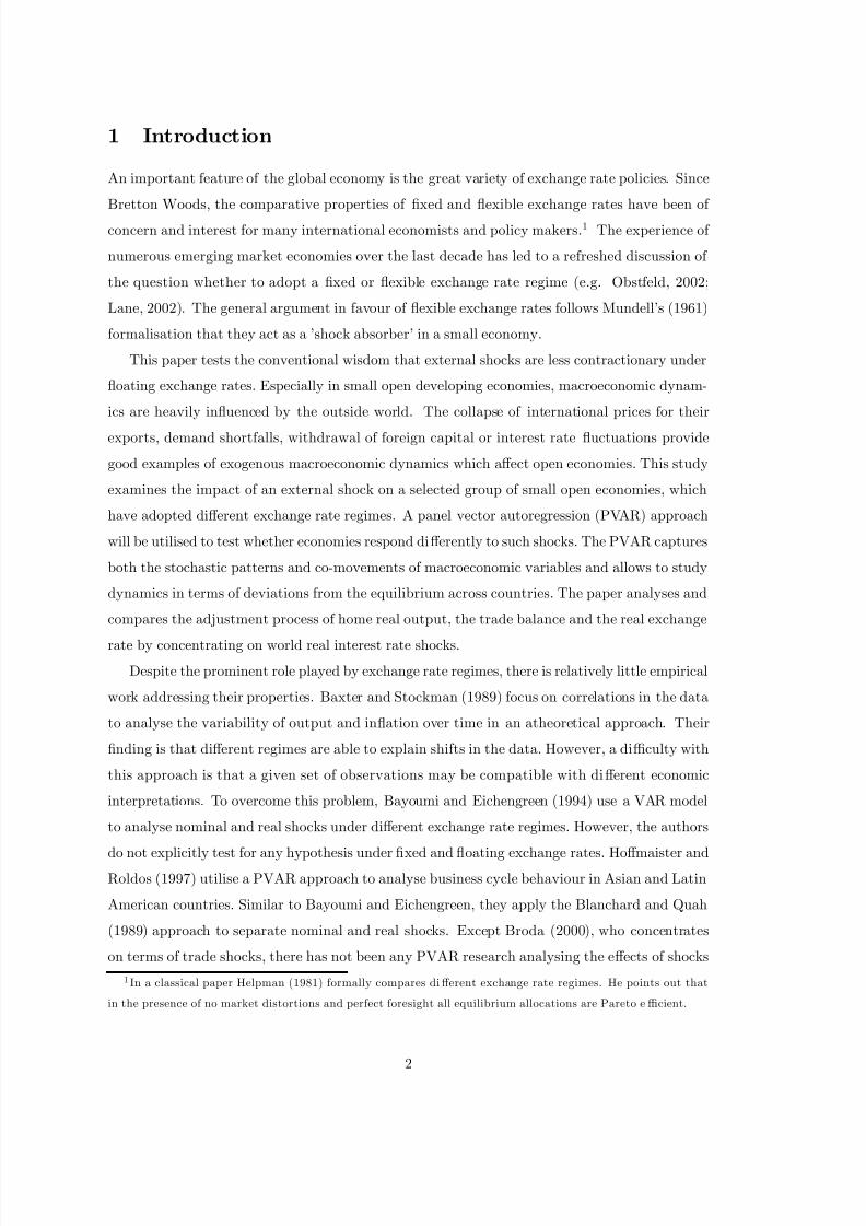
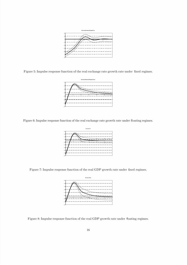
Figures 1 to 6 show the responses of the complete sample under the de facto speci fication of

Reinhart and Rogoff (2002) to the one period one hundred basis point rise in the world real

interest rate. Figure 1 depicts the adjustment process of real output in the fixed exchange rate

economies. After an initial positive impact eff ect, the economy is pushed into recession in the

short-run, i.e. the first period of the shock. This negative eff ect of the external shock equates

to 0.05 percentage points and is statistically diff erent from zero. In the medium-run, the third

period after the shock, output growth declines again and reaches a negative growth rate of

0.01 percentage points. Overall, the adjustment process is relatively volatile. Figure 3 shows

the time path of the adjustment of the trade balance. The impulse response function suggests

that the adjustment process of the trade balance is only completed in the long-run, i.e. the

eighth period after the shock. After an initial deterioration, which is statistically significant, net

exports improve by 0.88 percentage points in the short-run. Thus, countries with a nominal fixed

exchange rate off -set the external shock to the trade balance by increasing their exports relative

to their import demands in the short-run. The real exchange rate response is outlined in Figure

5. Initially, the real exchange rate appreciates before slowly moving towards a real depreciation of

0.13 percentage points in the second period after the shock. Overall, the responses are signi ficant

for the first two periods of the adjustment process. The adjustment process is completed in the

fifth period after the shock. The total long-run impact on the real exchange rate equals -1.5

percentage points (bottom panel of Table 5).

The analysis of the flexible exchange rate regimes illustrates that the eff ect of a one time

change of the world real interest rate on real output growth under floating exchange rates is

negative and significantly diff erent from zero in the initial period of the shock (Figure 2). The

economy moves into recession. The real GDP growth rate declines by 0.33 percentage points. In

17 The estimation strategy of dynamic panel data dep ends on the error term being serially uncorrelated. Several

tests of normality are applied to validate the choice of the estimation approach (e.g. Holtz-Eakin, 1988). Results

are available on request.18 The confidence intervals were computed using the approach by Luetkepohl (1990).

8



the medium-run, real GDP growth returns to its pre-shock level. Overall, the adjustment process

is less volatile than under fixed exchange rate regimes. Figure 4 illuminates the behaviour of the

trade balance to the shock of the world real interest rate. The trade balance instantaneously

improves by 0.02 percentage points. In the following periods the trade balance improves further

and remains in surplus. Only the short-run and second period improvements of net exports

by 0.28 and 0.1 percentage points remain statistically significant. The adjustment process is

completed after five years. This is in contrast to the trade balance response under the fixed

exchange rate regimes. Figure 6 depicts the real exchange rate response to the external shock.

The real exchange rate depreciates strongly in the short-run, although it is subject to an initial

appreciation. The real exchange rate in a floating exchange rate regime behaves markedly in

contrast to the pegging exchange rate regimes. The short-run depreciation of 0.55 percentage

points is statistically diff

erent from zero. The accumulated long-run impact of the world realinterest rate shock on the real exchange rate equals 0.72 percentage points, as illustrated in the

bottom panel of Table 5.

The real exchange rate response gives empirical validity to the theoretical proposition that

under floating exchange rate regimes the real exchange rate should depreciate more strongly.

It is also found that the adjustment process of the trade balance lasts longer under pegs than

under floats. Floating regimes are able to smooth eff ects of negative real shocks on real GDP

growth by utilising the nominal exchange rate as a shock absorber. By contrast, the growth rate

of real GDP under pegging exchange rate regimes needs a longer time horizon of adjustment and

reflects a higher volatility during the process of adjustment.19

Statistical diff erences between the estimated coefficients of the two regimes also play an

important role in the analysis. Tables 5 present Wald tests which report the joint significance

of the diff erence between the floating and pegged coefficients from the VAR in conjunction with

the estimated accumulated coefficients of the impulse response process for the adjustment of

the variables of interest. The bottom panel of Table 5 illustrates that the accumulated total

responses of the real exchange rate are in line with the predictions that the real exchange rate

depreciates more strongly under floats and, hence, allows the trade balance to adjust faster under

floats. However, an examination of the real output response in the top panel of Table 5 reveals

that the accumulated long-run response of real GDP is less contractionary under fixed exchange

rate regimes on the whole. A statistical diff erence of the floating and pegged coefficients is found

for the trade balance and real exchange rate variables (medium and bottom panel of Table 5).

19 The results do not vary significantly if sub-samples of financially or trade-open countries are considered (see

Hoff mann, 2002).

9



4.1.1 De Jure Specification

This subsection replicates the analysis for the de jure specification. The previous findings of

the evolution of real output are revised in Figures 7 and 8 since the actual and publicly stated

behaviours do not necessarily coincide. Under fixed and floating exchange rate regimes the

economy initially moves into recession. The recessionary impact is more pronounced under pegs

than under floats (see top panel of Table 6). Nevertheless, in the short-run both regimes recover.

The process of recovery is clearly more accentuated under floating exchange rate regimes. The

negative accumulated eff ect on the real GDP growth rate in the medium-run is equal to 0.17

percentage points under pegs, while the positive accumulated eff ect of real output under floats

equals 0.6 percentage points. Wald tests, which evaluate diff erences between the world real

interest rate and GDP coefficients respectively, generate statistical significance (top panel of

Table 6).

The behaviour of net exports are described in Figures 9 and 10. The initial trade balance

eff ect is negative in the pegging countries. The first four p eriods after the shock are statistically

significant. The trade balance improves only in the second period after the shock. Overall, the

trade balance deteriorates by 0.9 percentage points (medium panel of Table 6) and is relatively

volatile. Under floats net exports follow a diff erent adjustment pattern. After an initial im-

provement net exports remain in surplus. Overall, an accumulated trade balance surplus of 0.76

percentage points is established in the long-run (medium panel of Table 6). The Wald test of

the diff erences in all trade balance coefficients is statistically significant.The adjustment process of the real exchange rate is portrayed in Figures 11 and 12. The

instantaneous real exchange rate movements illuminate a negative eff ect in floating exchange rate

economies. Under fixed exchange rate regimes the real exchange rate depreciates instantaneously

and the rise of the real exchange rate reaches its peak during the first period. Under floats a real

depreciation occurs in the first period. However, the real exchange rate depreciation is stronger

in the fixed exchange rate economy. The overall accumulated impact on the real exchange rate

is presented in the bottom panel of Table 6, which illustrates a stronger positive eff ect under

fixed exchange rate regimes. This is in contrast to the de facto analysis. Again, Wald tests of

the diff erence between the real exchange rate coefficients are significant at the one percent level

(bottom panel of Table 6).

10



5 Conclusion

In order to meaningfully add to the debate whether fixed or floating exchange rate regimes are

superior, this paper examines the theoretical hypothesis that nominal exchange rates act as a

shock absorber under floating exchange rate regimes. The paper utilises a Panel VAR approach.

The empirical results provide support for the predictions of the literature on exchange rate

regimes. Given a shock to the world real interest rate, the paper confirms for the de facto

sample that the adjustment process of real GDP is more volatile under pegs. Real exchange

rate movements in form of a real depreciation are stronger under floats. Hence, a smooth trade

balance adjustment is achieved more quickly under floating exchange rate regimes. The de jure

specification confirms the results for the evolution of real output and the trade balance. Overall,

the contrasts between the two exchange rate regimes are more pronounced under the de jure

specification.

11



References

[1] Barro, R. and Sala-i-Martin, X. (1990), ”World Real Interest Rates”, NBER Working Paper

3317.

[2] Baxter, M. and Stockman, A. (1989), ”Business Cycles and the Exchange Rate Regime:

Some International Evidence”, Journal of Monetary Economics 23: 377-400.

[3] Bayoumi, T. and Eichengreen, B. (1994), ”Macroeconomic Adjustment under Bretton

Woods and the Post-Bretton-Woods Float: An Impulse-Response Analysis”, Economic

Journal 104: 813-827.

[4] Bergin, P. (2001), ”Putting the ‘New Open Economy Macroeconomics’ to a Test”, mimeo,

University of California at Davis.

[5] Bergin, P. and Sheff rin, S. (2000), ”Interest Rates, Exchange Rates and Present Value

Models of the Current Account”, Economic Journal 110: 535-558.

[6] Blanchard, O.J. and Quah, D. (1989), ”The Dynamic Eff ects of Aggregate Demand and

Supply Disturbances”, American Economic Review 79: 655-673.

[7] Broda, C. (2000), ”Terms of Trade and Exchange Rate Regimes in Developing Countries”,

mimeo, MIT.

[8] Chiang, M. H. and Kao, C. (2000), ”Nonstationary Panel Time Series Using NPT 1.2- A

User Guide”, mimeo, Syracuse University.

[9] Frankel, J.A. (1999), ”No Single Currency Regime is Right for all Countries or at all Times”,

NBER Working Paper 7338.

[10] Frankel, J.A. and Romer, D. (1999), ”Does Trade Cause Growth?”, American Economic

Review 89: 379-399.

[11] Friedman, M. (1953), ”The Case for Flexible Exchange Rates”, in: Essays in Positive

Economics , University of Chicago, Chicago.

[12] Helpman, E. (1981), ”An Exploration in the Theory of Exchange Rate Regimes”, Journal

of Political Economy 89: 865-890.

[13] Hoff maister, A.W. and Roldos, J.E. (1997), ”Are Business Cycles Diff erent in Asia and

Latin America?”, IMF Working Paper 97/9.

12



[14] Hoff mann, M. (2002), ”Fixed versus Flexible Exchange Rates: Theory and Empirical Evi-

dence, mimeo, University of Cologne.

[15] Holtz-Eakin, D. (1988), ”Testing for Individual Eff ects in Autoregressive Models”, Journal

of Econometrics 39: 297-307.

[16] International Monetary Fund (2000), International Financial Statistics: CD-Rom , Wash-

inghton D.C..

[17] International Monetary Fund (2000), Annual Report on Exchange Arrangements and Ex-

change Restrictions , Washington D.C..

[18] Lane, P.R. (2002), ”Business Cycles and Macroeconomic Policy in Emerging Market Eco-

nomics”, mimeo, Trinity College Dublin.

[19] Lane P. and Milesi-Feretti, G. M. (2002), ” External Wealth, the Trade Balance and the

Real Exchange Rate”, Forthcoming in European Economic Review .

[20] Levin, A. and Lin, C.F. (1992), ”Unit Root Test in Panel Data: Asymptotic and Finite

sample Properties”, University of San Diago Discussion Paper 92-93.

[21] Luetkepohl, H. (1990), ”Asymptotic Distributions of Impulse Response Functions and Fore-

cast Error Variance Decomposition of Vector Autoregressive Models”, Review of Economics

and Statistics 72: 116-125.

[22] McCoskey, S. and Kao, C. (1998), ” A Residual Based Test of the Null of Cointegration in

Panel Data”, Econometric Reviews 17: 57-84.

[23] Mundell, R.A. (1961), ”A Theory of Optimum Currency Areas”, American Economic Re-

view 51: 657-665.

[24] Obstfeld, M. (2002), ”Exchange Rates and Adjustment: Perspectives from the New Open

Economy Macroeconomics”, mimeo, University of California, Berkley.

[25] Obstfeld, M. and Rogoff , K. (1995), ”The Intertemporal Approach to the Current Account,”

in: Handbook of International Economics vol. 3 , edited by G. Grossman and K. Rogoff ,

North-Holland.

[26] Reinhart, C. M. and Rogoff , K. (2002), ”The Modern History of Exchange Rate Arrange-

ments: A Reinterpretation”, NBER Working Paper 8963.

13



[27] Taylor, J.B. (1989), ”Policy Analysis with a Multicountry Model”, in: Macroeconomic Poli-

cies in an Interdependent World , edited by R.C. Bryant, D.A. Currie, J.A. Frenkel, P.R.

Masson and R. Portes, Washington D.C., IMF, 122-142.

[28] World Bank (2001) World Development Indicators CD-Rom , Washington D.C..

14



De Facto (Reinhart & Rogoff): Fix

-0.4

-0.3

-0.2

-0.1

0

0.1

0.2

0.3

0.4

0 1 2 3

Figure 1: De Facto: Impulse response function of the real GDP growth rate under fixed regimes.

De Facto (Reinhart & Rogoff): Float

-0.4

-0.35

-0.3

-0.25

-0.2

-0.15

-0.1

-0.05

0

0.05

0.1

0.15

0.2

0.25

0 1 2

Figure 2: Impulse response function of the real GDP growth rate under floating regimes.


-1.2

-1

-0.8

-0.6

-0.4

-0.2

0

0.2

0.4

0.6

0.8

1

1.2

0 1 2 3 4 5 6 7

Figure 3: Impulse response function of the growth in net exports under fixed regimes.


-0.15

-0.05

0.05

0.15

0.25

0.35

0 1 2 3 4 5

Figure 4: Impulse response function of the growth in net exports under floating regimes.

15




-1.2

-1

-0.8

-0.6

-0.4

-0.2

0

0.2

0.4

0 1 2 3 4

Figure 5: Impulse response function of the real exchange rate growth rate under fixed regimes.


-0.7

-0.5

-0.3

-0.1

0.1

0.3

0.5

0.7

0 1 2 3 4 5

Figure 6: Impulse response function of the real exchange rate growth rate under floating regimes.

De Jure: Fix

-0.55

-0.45

-0.35

-0.25

-0.15

-0.05

0.05

0.15

0.25

0.35

0 1 2 3 4 5

Figure 7: Impulse response function of the real GDP growth rate under fixed regimes.

De Jure: Float

-0.25

-0.15

-0.05

0.05

0.15

0.25

0.35

0.45

0.55

0 1 2 3 4 5

Figure 8: Impulse response function of the real GDP growth rate under floating regimes.

16



De Jure: Fix

-0.8

-0.6

-0.4

-0.2

0

0.2

0.4

0 1 2 3 4 5 6 7

Figure 9: Impulse response function of the growth in net exports under fixed regimes.

De Jure: Float

-0.05

0

0.05

0.1

0.15

0.2

0.25

0.3

0.35

0.4

0.45

0 1 2 3 4 5

Figure 10: Impulse response function of the growth in net exports under floating regimes.

De Jure: Fix

-0.1

-0.05

0

0.05

0.1

0.15

0.2

0.25

0.3

0.35

0.4

0.45

0.5

0 1 2 3

Figure 11: Impulse response function of the real exchange rate growth rate under fixed regimes.

De Jure: Float

-0.25

-0.2

-0.15

-0.1

-0.05

0

0.05

0.1

0.15

0.2

0.25

0 1 2 3 4

Figure 12: Impulse response function of the real exchange rate growth rate under floating regimes.

17



Sample of Countries

Argentina Dominican Republic Jordan Paraguay TunisiaBahrain Ecuador Korea Peru TurkeyBolivia Egypt Malaysia Philippines Trinidad and TobagoBotswana El Salvador Mauritius Saudi Arabia UruguayBrazil Guatemala Mexico Singapore VenezuelaChile India Morocco South Africa ZimbabweColombia Indonesia Oman Sri LankaCosta Rica Israel Pakistan SyriaCote D’Ivore Jameica Panama Thailand

Table 1: Country List

VariablesLevin and Lin Test

Levels: tRh o criticalProb. First Di ff erences: tRh o criticalProb.

Real GDP (Level) 0.291 0.418 ∆Real GDP -58.97 0.000

Real Exchange Rate (Level) 0.376 0.395 ∆Real Exchange Rate -152.58 0.000

Net Exports (Levels) 0.825 0.314 ∆Net Exports -180.75 0.000

World Interest Rate (Level) 0.078 0.478 ∆World Interest Rate -166.07 0.000

World Real GDP (Level) 0.24 0.432 ∆World Real GDP -60.59 0.000

Table 2: Panel Unit Root Test. Note: The null hypothesis is that the series is nonstationary.

Variables (Relation)Mc Coskey and Kao

LM Plus Test Real GDP: 38.827 (0.0000) (reject)World Real GDP→World Interest Rate→Net Exports→Real Exchange Rate

Real Exchange Rate: 26.268 (0.0000) (reject)

World Real GDP→

World Interest Rate→Net Exports→Real GDP

Net Exports: 26.495 (0.0000) (reject)World Real GDP→World Interest Rate→Real Exchange Rate→Real GDP

Table 3: Residual Based Cointegration Test. Note: The null hypothesis is that there is cointe-

gration (no unit root in the errors). The critical probabilities are in parentheses.

18



Variables

Complete Sample Mean StDev Max MinFix: De JureReal GDP 0.045 0.05 0.22 -0.14

Net Exports 0.001 0.06 0.21 -0.23

RER 0.0012 0.10 0.62 - 0.39Float: De JureReal GDP 0.038 0.04 0.12 -0.14

Net Exports 0.002 0.04 0.21 -0.14

RER 0.021 0.13 1.05 -0.38

Fix: De FactoReal GDP 0.039 0.05 0.17 -0.14

Net Exports -0.0003 0.05 0.17 -0.23

RER 0.007 0.08 0.48 -0.18Float: De FactoReal GDP 0.040 0.04 0.17 -0.13

Net Exports 0.0003 0.03 0.20 - 0.17

RER 0.01 0.12 0.81 -0.38

Table 4: Summary Statistic. Note: Obtained from fi rst di ff erenced variables in the system.

19



Elasticities Real Output

Wald-Test Float Fixed All WIR Coeff . χ2(4) 2.39

All Coeff . χ2(13) 6.02

Impact -0.331 0.235(0.024) (0.025)

Medium-Run -0.329 0.205(1.165) (1.669)

Long-Run -0.329 0.208(1.164) (1.669)

Elasticities Net ExportsWald-Test Float Fixed

All WIR Coeff . χ2(4) 8.58∗

All Coeff . χ2(13) 14.82

Impact 0.023 -0.856(0.055) (0.046)

Medium-Run 0.438 1.145(0.297) (0.768)

Long-Run 0.453 2.442(0.30) (0.761)

Elasticities Real Exchange RateWald-Test Float Fixed

All WIR Coeff . χ2(4) 12.08∗∗∗

All Coeff . χ2(13) 47.59∗∗∗

Impact -0.565 -1.029(0.017) (0.068)

Medium-Run 0.483 -1.522(0.541) (1.304)

Long-Run 0.716 -1.508(0.543) (1.299)

Sample Size 724Estimation Period 1974-99

Table 5: Accumulated Coefficients of Real GDP, Net Exports and the Real Exchange Rate on the

De Facto Estimation to a Positive Shock to the World Real Interest Rate. Note: All countries.

Standard errors in parentheses. Wald Test for the joint signi fi cance of the di ff erence of the peg and fl oat coe ffi cients of real output, net exports and real exchange rate equation respectively. (.)

imply the number of restrictions. *** Represence of signi fi cance at the 1 percent, ** at the 5

percent, * at the 10 percent level. The medium-run re fl ects three years and the long-run eight

years after the shock.

20



Real Output

Wald-Test Float Fixed All WIR Coeff . χ2(4) 7.78∗

All Coeff . χ2(13) 36.11∗∗∗

Impact -0.154 -0.499(0.012) (0.011)

Medium-Run 0.591 -0.166(0.373) (0.238)

Long-Run 0.655 -0.159(0.371) (0.236)

Elasticities Net ExportsWald-Test Float Fixed

All WIR Coeff . χ2(4) 6.55

All Coeff . χ2(13) 29.49∗∗∗

Impact 0.158 -0.503(0.017) (0.046)

Medium-Run 0.724 -0.952(0.046) (0.132)

Long-Run 0.763 -0.902(0.041) (0.125)

Elasticities Real Exchange RateWald-Test Float Fixed

All WIR Coeff . χ2(4) 31.03∗∗∗

All Coeff . χ2(13) 62.11∗∗∗

Impact -0.171 0.093(0.0131) (0.012)

Medium-Run 0.04 0.602(0.126) (0.153)

Long-Run 0.04 0.613(0.124) (0.154)

Sample Size 629Estimation Period 1974-99

Table 6: Accumulated Coefficients of Real GDP, Net Exports and the Real Exchange Rate on

the De Jure Estimation to a Positive Shock to the World Real Interest Rate. Note: All countries.

Standard errors in parentheses. Wald Test for the joint signi fi cance of the di ff erence of the peg and fl oat coe ffi cients of real output, net exports and real exchange rate equation respectively. (.)

imply the number of restrictions. *** Represence of signi fi cance at the 1 percent, ** at the 5

percent, * at the 10 percent level. The medium-run re fl ects three years and the long-run eight

years after the shock.

21

fixed versus flexible exchange rates: a panel-var

Documents