Fiscal Sustainability, Public Investment, and

Growth in Natural Resource-Rich, Low-Income

Countries: The Case of Cameroon

Issouf Samake, Priscilla Muthoora, and Bruno Versailles

WP/13/144

© 2013 International Monetary Fund WP/13/144

IMF Working Paper

African Department

Fiscal Sustainability, Public Investment, and Growth in Natural Resource-Rich, Low-

Income Countries: The Case of Cameroon

Prepared by Issouf Samake, Priscilla Muthoora, and Bruno Versailles1

Authorized for distribution by Mario de Zamaróczy

June 2013

1 The authors wish to thank Mario de Zamaróczy and Mauro Mecagni for their guidance and very helpful discussions. We

also thank Alfredo Baldini, Andy Berg, Katja Funke, Bin Li, Paolo Mauro, Giovanni Melina, Fabien Nsengiyumva, Alex

Segura-Ubiergo, Jean van Houtte, Susan Yang and Felipe Zanna for useful comments. Any errors and omissions are the

authors’ sole responsibility.

This Working Paper should not be reported as representing the views of the IMF.

The views expressed in this Working Paper are those of the authors and do not necessarily

represent those of the IMF or IMF policy. Working Papers describe research in progress by

authors and are published to elicit comments and to further debate.

Abstract

This paper assesses the implications of the use of oil revenue for public investment on

growth and fiscal sustainability in Cameroon. We develop a dynamic stochastic general

equilibrium model to analyze the effects of such investment on growth and on the path of key

fiscal indicators, such as the non-oil primary deficit and public debt. Policy scenarios show

that Cameroon’s large infrastructural needs and relatively low current debt levels could

justify a temporary deviation from traditional policy advice that suggests saving part of the

oil revenue to smooth expenditure over time. Model simulations show that a relatively high

degree of efficiency of public investment is needed for scaled-up public investment to make a

significant contribution to growth, while maintaining fiscal sustainability.

JEL Classification Numbers: C11, C15, C61, E22, E23, E27, H61, O11

Keywords: Cameroon, fiscal policy, DSGE, natural resource-rich countries, low-income

countries, public investment, growth.

Author’s email address: isamake@imf.org; pmuthoora@imf.org; bversailles@imf.org

2

Contents

I. Introduction ........................................................................................................................... 3

II. Literature Review: Revenue Management from Non-Renewable Natural Resources ......... 6

III. Cameroon: Experience and Issues ...................................................................................... 8

IV. The Model ......................................................................................................................... 11

A. Representative Agent Maximization Problem ......................................................... 12 B. Production ................................................................................................................ 13 C. Fiscal Policy and the Ramsey Problem .................................................................... 15

V. Model Calibration and Simulation Method ....................................................................... 17

VI. Results of Policy Scenarios .............................................................................................. 21

A. “Scaling-Up with Reform” Scenario ........................................................................ 21

B. “Conservative” Scenario .......................................................................................... 21 C. “Scaling-Up No Reform” Scenario .......................................................................... 25

VII. Conclusion and Policy Implications ................................................................................ 25

Appendix

First Order Conditions ............................................................................................................ 27

References ............................................................................................................................... 30

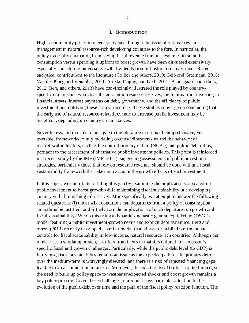
3

I. INTRODUCTION

Higher commodity prices in recent years have brought the issue of optimal revenue

management in natural resource-rich developing countries to the fore. In particular, the

policy trade-offs emanating from saving fiscal revenue from oil resources to smooth

consumption versus spending it upfront to boost growth have been discussed extensively,

especially considering potential growth dividends from infrastructure investment. Recent

analytical contributions to the literature (Collier and others, 2010; Gelb and Grasmann, 2010;

Van der Ploeg and Venables, 2011; Arezki, Dupuy, and Gelb, 2012; Baunsgaard and others,

2012; Berg and others, 2013) have convincingly illustrated the role played by country-

specific circumstances, such as the amount of resource reserves, the returns from investing in

financial assets, interest payments on debt, governance, and the efficiency of public

investment in amplifying these policy trade-offs. These studies converge on concluding that

the early use of natural resource-related revenue to increase public investment may be

beneficial, depending on country circumstances.

Nevertheless, there seems to be a gap in the literature in terms of comprehensive, yet

tractable, frameworks jointly modeling country idiosyncrasies and the behavior of

macrofiscal indicators, such as the non-oil primary deficit (NOPD) and public debt ratios,

pertinent to the assessment of alternative public investment policies. This point is reinforced

in a recent study by the IMF (IMF, 2012), suggesting assessments of public investment

strategies, particularly those that rely on resource revenue, should be done within a fiscal

sustainability framework that takes into account the growth effects of such investment.

In this paper, we contribute to filling this gap by examining the implications of scaled-up

public investment to boost growth while maintaining fiscal sustainability in a developing

country with diminishing oil reserves. More specifically, we attempt to answer the following

related questions: (i) under what conditions can departures from a policy of consumption

smoothing be justified; and (ii) what are the implications of such departures on growth and

fiscal sustainability? We do this using a dynamic stochastic general equilibrium (DSGE)

model featuring a public investment-growth nexus and explicit debt dynamics. Berg and

others (2013) recently developed a similar model that allows for public investment and

controls for fiscal sustainability in low-income, natural resource-rich countries. Although our

model uses a similar approach, it differs from theirs in that it is tailored to Cameroon’s

specific fiscal and growth challenges. Particularly, while the public debt level (to GDP) is

fairly low, fiscal sustainability remains an issue as the expected path for the primary deficit

over the medium-term is worryingly elevated, and there is a risk of repeated financing gaps

leading to an accumulation of arrears. Moreover, the existing fiscal buffer is quite limited, so

the need to build up policy space to weather unexpected shocks and boost growth remains a

key policy priority. Given these challenges, our model pays particular attention to the

evolution of the public debt over time and the path of the fiscal policy reaction function. The

4

latter is rule-based (automatic tax and expenditure responses to economic activity), but it also

allows for discretionary shocks (systematic and random) in which the fiscal buffer plays a

role. In this framework, the model attempts to balance the need to boost growth through

public investment (complemented by private investment), which is constrained by the limited

buffer and a declining oil endowment, with the need to maintain debt at a sustainable level by

keeping the primary deficit in check.

The model is calibrated to Cameroon and simulates three policy scenarios in 2012–

32: (i)“scaling-up with reform” scenario, (ii) “conservative” scenario; and (iii) “scaling-up no

reform” scenario.2 During this period, the oil price is forecast to be between US$95–110 a

barrel and oil reserves are assumed to be depleted by 2032.

The “scaling-up with reform” scenario assumes that public investment will increase

steadily to 12 percent of GDP by 2032 (from 6.5 percent of GDP in 2012).3 The

investment will be financed through oil revenue, and additional borrowing if

necessary (as the oil endowment depletes overtime).4 Borrowing may occur if

existing fiscal buffers (measured by government cash deposits at the central bank)

would not suffice because oil revenue is projected to decline. The scenario also

assumes an improvement in the efficiency of public investment relative to

Cameroon’s historical average; similar to the median middle-income countries’

efficiency levels. The reform element of the scenario incorporates the assumption that

structural impediments are lifted in order to ensure that a greater share of public

investment translates into effective capital stock.

The “conservative” scenario assumes that public investment will remain broadly

similar to its 2012 level in terms of GDP. It also assumes similar improvements in the

efficiency of public investment as in the “scaling-up with reform” scenario. Because

oil production is projected to decline (along with assumed limited fiscal space,

limited possibility to tap the international financial market, and prospective financial

difficulties associated with declining oil revenue), we also expect tighter financial

constraints during 2012–32.

2 Recent explorations give some indications that oil reserves may not necessarily be fully depleted by 2032.

However, this would not fundamentally alter the qualitative assessment that Cameroon’s reserves are on a

declining path.

3 Reflecting complementarities between public and private capital, private investment is expected to increase

overtime.

4This assumption is consistent with the Cameroonian authorities’ vision expressed in Cameroon’s Growth and

Employment Strategy Paper (Government of Cameroon, 2009).

5

The “scaling-up no reform” scenario assumes no change in public investment

efficiency relative to its historical level, with investment similar to the one in the

“scaling-up with reform” scenario. This implies that public investment efficiency is

lower than in the other two scenarios, which is consistent with observations in several

other low-income countries that do not (or slowly) enact structural reforms.

Our work complements existing analysis by making two key contributions. First, our

modeling strategy specifically tracks a reaction function for fiscal policy with explicit public

debt dynamics. It differs from standard approaches for the optimal path of government

spending from resource revenue, such as the Permanent Income Hypothesis (PIH), in that the

PIH is purely forward looking, while our model takes into account constraints facing the

government by looking at past government behavior. Specifically, in the PIH approach, the

present value of the resource wealth is the only binding constraint on spending. By contrast,

our reaction function approach takes a broader view by including the need to build fiscal

buffers. Second, we quantify the importance of public capital efficiency in determining the

growth returns of public infrastructure. This consideration is crucial because inefficiencies

related to public investment can be an important channel for the transmission of the “resource

curse.” Dabla-Norris and others (2011), for example, find a negative correlation between

their index of public investment quality and natural resource dependence.

Overall, policy experiments show that Cameroon’s large infrastructural needs could justify a

deviation from the PIH approach, and support a gradual scaling up of public investment,

provided its effectiveness is simultaneously enhanced. In the “scaling-up with reform”

scenario, the public investment efficiency parameter is set at 0.54, and real GDP growth

averages 5.1 percent a year in 2012–32, which is 2.3 percentage points higher than the

average in 2006–11. The other two scenarios yield smaller growth gains and worse fiscal

outcomes (in terms of the NOPD and debt). Our results, generally, show that efficiency

matters for growth; hence, while low-income, natural resource-rich countries could benefit

from using their resource revenue to scale up public investment, efforts are needed to

enhance the effectiveness of their public investment simultaneously to achieve sustainable

and higher growth rates.

The rest of the paper is organized as follows. Section II presents a selective review of the

existing literature. Section III discusses Cameroon’s experience with natural resource

revenue. Section IV lays out the model. The model calibration and simulation are developed

in Section V. Section VI discusses results of the three scenarios. Section VII provides

concluding remarks.

6

II. LITERATURE REVIEW: REVENUE MANAGEMENT FROM NON-RENEWABLE NATURAL

RESOURCES

A large body of literature proposes policy recommendations on the use of natural resource

revenue. This literature is dominated by the PIH approach, which recommends that

governments smooth primary expenditure over time, setting it equal to their permanent

income (i.e., the constant level of fiscal revenue that can be generated from natural resources

and other revenue).5 In other words, the PIH approach implies setting a target NOPD at the

level of the permanent income from all sources. Operationally, the PIH implies that resource

revenue is saved in the early years of extraction, and such reserves will be gradually run

down as resource depletion takes place. In this sense, the policy prescription of the PIH

involves both stabilization, through the avoidance of procyclical policies because of resource

price volatility, and intergenerational equity, through the saving of resource wealth for future

generations.

Uncertainty over the determination of the permanent income remains nevertheless a key

obstacle in the implementation of expenditure smoothing according to the PIH.

Consequently, the Bird-in-Hand (BIH) approach has been proposed. Compared to the PIH,

the BIH approach is more conservative, because it implies a higher rate of savings from

resource revenue and is based on financial returns on liquidated resource wealth, not

identified natural resource reserves. Specifically, a BIH rule requires countries to use all

resource-related revenue to accumulate financial assets and use only the yield from the

accumulated financial assets to finance expenditure. Thus, the BIH approach is quite

restrictive, particularly in the initial years of resource exploration when the accumulated

financial wealth is low. Katz and others (2004) argue that the BIH approach has several

advantages over the PIH approach: increasing expenditure over time, which is politically

more appealing than keeping it constant at the assumed permanent income level, and

providing more effective stabilization to expenditures since these are based on predictable

revenue flows. Norway is a prominent example for the application of the BIH approach.6

There are growing concerns, however, that the policy prescriptions of the PIH or the BIH

approaches, while optimal in an intertemporal consumption smoothing sense, may be

misguided for the use of natural resource revenue. In particular, both approaches treat all

government spending as consumption and fail to distinguish between expenditure categories

5 See for example Barnett and Ossowski (2003), and Segura (2006).

6 In 2001, the Norwegian government implemented a BIH fiscal rule allowing the government to take out

4 percent of the value of the oil saving fund in the previous year, equivalent to the real return on the fund, to

finance the general government budget in the current year (Bjerkholt and Niculescu, 2004 ; Harding and

Van der Ploeg, 2009).

7

such as investment abroad and investment at home, and their effects on growth, especially in

credit-constrained economies (IMF, 2012). Consequently, fiscal policies based on these

approaches may result in suboptimal public investment levels. This is partly because of

(i) limited attention to constraints and incentives facing policymakers;7 and (ii) the focus on a

single target to serve as the fiscal anchor (for example the permanently sustainable NOPD in

the case of the PIH), while fiscal sustainability and growth concerns are not necessarily fully

addressed.

Several papers have addressed these concerns. Takaziwa, Gardner, and Ueda (2004), for

example, consider whether countries are better off spending their resource wealth upfront.

They show that if the quality of public investment is high enough to boost productivity, the

optimal short-run level of government spending in a capital-scarce economy is higher than

what the standard PIH prescription suggests.

Collier, and others (2010) consider multiple options for natural resource revenue-financed

government spending, which they summarize as follows: (i) distribute government resource

revenue to households through cash transfers or reduce taxes for households and/or

companies; (ii) increase spending on public consumption or investment; (iii) retain resources

as government financial assets and lend on to the domestic private sector (possibly through

lowering public debt); and (iv) lend to foreigners. They argue that the optimal rate of saving

from natural resource revenue depends not only on permanent income, but also on other

factors, such as the spread between the current price and the long-run price for the resource;

the degree of capital scarcity in the country; and the level of external indebtedness of the

government. Specifically, their framework characterizes optimal policy, given borrowing

costs, interest premiums on debt, and capital scarcity, as follows: (i) if smoothing aggregate

consumption is an objective of the government, this can be achieved through initial

borrowing and eventual payment of dividends from interest on saved revenue; (ii) if the

interest on foreign debt exceeds the return on assets, resource revenue should be used to pay

off the debt; and (iii) natural resource revenue should be used for investment in infrastructure

rather than for foreign financial assets in capital-scarce countries.

Arezki, Dupuy, and Gelb (2012) show analytically that these conclusions need to be nuanced

because weaker administrative capacity undermines the increase in optimal public capital

spending in the aftermath of a resource boom. This can however be mitigated by high total

factor productivity. Furthermore, in the presence of adjustment costs that are increasing with

the size of spending induced by natural resource revenue, redistribution to the private sector

may be preferable to a scaling up of public investment.

7 For a discussion of fiscal anchors in resource-rich developing countries, see Baunsgaard and others (2012) and

IMF (2012).

8

Unlike the standard PIH approach, recent work at the IMF (IMF, 2012; Berg and others,

2013) argues for a more integrated framework that explicitly accounts for the return on

public investment and fiscal sustainability. Furthermore, increasing attention, particularly in

policy circles, is being paid to the implications of going beyond the standard consumption-

savings/investment analytical frameworks for fiscal policy and external sector assessments.

The recent IMF papers acknowledge the importance of the efficient use of public

investment.8 We take a similar stance in our model with particular emphasis on the size of

public investment and its effectiveness, as well as its effects on growth. In doing so, we focus

on the key constraints on the scaling up of government investment, notably past fiscal policy

implementation, limits to debt financing, and the efficiency of public investment. In

particular, as in IMF (2012), our model emphasizes the role of public investment both

through its size and effectiveness to assess its contribution to growth.

III. CAMEROON: EXPERIENCE AND ISSUES

In the last 30 years, Cameroon has experienced moderate growth with limited improvement

in socioeconomic indicators. Economic activity contracted sharply between 1977, when oil

production started, and 1986, when it peaked.9 The resulting fall in per capita income

contributed to large-scale poverty and disappointing human development indicators.10

Cameroon’s proven oil reserves are relatively small, and its economy is more diversified than

those of neighboring oil-producing countries.11 As recognized in Berg and others (2013), the

small reserve endowment and the associated short-term horizon further amplify the fiscal

challenges. Contractual arrangements between international oil companies and the

8 Public investment efficiency is defined as the ratio of public investment spending to the value of resulting

installed public capital. In general, in environments of imperfect information and/or governance constraints,

projects with the highest returns are not necessarily chosen, and, not always well executed. A complementary

way to think about efficiency is that a fraction of spending is wasted through suboptimal project execution

processes (e.g., procurement issues).

9 Gauthier and Zeufack (2009), for example, find that GDP contracted on average by 5 percent a year between

1977 and 1985, or by a cumulative 27 percent during the period. Arbache and Page (2007), using event history

analysis, estimate that a growth deceleration occurred in 1986. The methodology and criteria they employ

suggest that growth would have been contracting for at least three years before 1986.

10 According to Essama-Nssah and Bassolé (2010), real GDP in 1990 was 20 percent lower than its 1985 level;

and per capita income fell by 50 percent between 1986 and 1993. Gauthier and Zeufack (2009) report that

Cameroon was poorer in 2007 than in 1986 in terms of GDP per capita (measured in constant 2000 U.S.

dollars).

11 In 2010, Cameroon’s oil production amounted to 63,800 barrels a day. Oil exports were about half of total

exports, while oil revenue was 27 percent of total government revenue. By comparison, in the same year,

Nigeria (sub-Saharan Africa’s largest oil producer) produced over 2.4 million barrels a day; oil exports were 96

percent of total exports; and oil revenue was 70 percent of total government revenue.

9

government ensure that a relatively high share of oil revenue accrues to the government as

royalties and taxes. Oil revenue was saved abroad in the early years of production and may

have been partly used to weather the economic crisis between 1985 and 1988 (Gauthier and

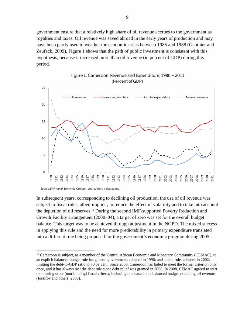
Zeufack, 2009). Figure 1 shows that the path of public investment is consistent with this

hypothesis, because it increased more than oil revenue (in percent of GDP) during this

period.

0

5

10

15

20

25

1980

1981

1982

1983

1984

1985

1986

1987

1988

1989

1990

1991

1992

1993

1994

1995

1996

1997

1998

1999

2000

2001

2002

2003

2004

2005

2006

2007

2008

2009

2010

2011

Figure 1. Cameroon: Revenue and Expenditure, 1980 – 2011

(Percent of GDP)

Oil revenue Current expenditure Capital expenditure Non-oil revenue

Source: IMF World Economic Outlook ; and authors' calculations.

In subsequent years, corresponding to declining oil production, the use of oil revenue was

subject to fiscal rules, albeit implicit, to reduce the effect of volatility and to take into account

the depletion of oil reserves.12 During the second IMF-supported Poverty Reduction and

Growth Facility arrangement (2000–04), a target of zero was set for the overall budget

balance. This target was to be achieved through adjustment in the NOPD. The mixed success

in applying this rule and the need for more predictability in primary expenditure translated

into a different rule being proposed for the government’s economic program during 2005–

12

Cameroon is subject, as a member of the Central African Economic and Monetary Community (CEMAC), to

an explicit balanced budget rule for general government, adopted in 1996; and a debt rule, adopted in 2002,

limiting the debt-to-GDP ratio to 70 percent. Since 2000, Cameroon has failed to meet the former criterion only

once, and it has always met the debt rule since debt relief was granted in 2006. In 2008, CEMAC agreed to start

monitoring other (non-binding) fiscal criteria, including one based on a balanced budget excluding oil revenue

(Iossifov and others, 2009).

10

08.13 Scheduled domestic debt/arrears repayments, rather than primary expenditure, were

designed as the adjustment variables in the face of financing constraints owing to changes in

international oil prices. Specifically, a slower pace of settlement of domestic debt/arrears

would accommodate lower-than-anticipated oil revenue and would offset the deterioration of

the overall balance. Conversely, oil revenue above the projected level was to be used to

accelerate domestic debt/arrears payments (Cossé, 2006). Overall, public capital expenditure

tracked oil sector revenue relatively closely in 1980–2011. However, since 1991, oil revenue

has been consistently higher than capital expenditure, implying that it was also used to

finance current spending or reserve building (Figure 1).

Given the above, the weak link between oil-financed public investment and growth in

Cameroon appears to be somewhat of a puzzle. Benjamin, Devarajan, and Weiner (1989)

have tried to explain this weak correlation with the “Dutch disease” effects of oil revenue.14

Gauthier and Zeufack (2009) argue that poor governance, which resulted in unproductive

capital spending, played a key role. They argue that, although much of the oil revenue during

Cameroon’s early years of production was saved abroad, there was little disclosure about its

actual magnitude. Their estimates suggest that a relatively large amount of this revenue (54

percent) cannot be accounted for. Another explanation, directly relevant to our analysis, is

the issue of the efficiency of public investment. Gupta and others (2011) find that adjusting

capital stocks for the efficiency of public investment15 amplifies the negative correlation

between resource rents and capital stocks found by Bhattacharya and Collier (2011). More

generally, Gupta and others (2011) find that controlling for efficiency reduces by more than

half the capital stock suggested by cumulative investment. Tabova and Baker (2011) find that

investment fails to spur growth in oil-producing countries in the CFA zone, citing the

inefficiency of investment and the lack of strong institutions and weak governance as

reasons.

13

Partly, this appears to have been the result of weak program ownership. In addition, the rule was applied on a

cash basis and was circumvented through the accumulation of domestic arrears during 2003–04 (Cossé, 2006).

14 The “Dutch disease” is defined as a series of negative consequences arising from large increases in a

country's foreign currency income. It is generally associated with a natural resource discovery, but can also arise

from any large increase in foreign currency earnings, including foreign direct investment, foreign aid, or a

substantial increase in natural resource prices. Typically, the Dutch disease results in a combination of (i) a

decline in price competitiveness, and thus exports, of the manufacturing sector; and (ii) an increase in imports.

The Dutch disease has generally been characterized as one of the root causes of the “natural resource curse.”

15

Gupta and others (2011) measure public investment efficiency using the Public Investment Management

Index (PIMI) as constructed by Dabla-Norris and others (2011). As such they make the assumption that not all

public investment spending translates fully into productive capital assets.

11

Between 2002 and 2011, the public investment-to-GDP ratio in Cameroon averaged

3.5 percent, compared to 10 percent in the Central African Economic and Monetary

Community (CEMAC), and more than 7 percent in sub-Saharan Africa (SSA).16 Apart from

the low efficiency of public investment translating into lower public capital stocks, public

investment budgets were also not being fully spent because of implementation problems.

This is related to low administrative capacity and recurring governance problems, as

acknowledged by recent initiatives including the setting up of a new ministry for public

procurement in 2012. Hence, preliminary results from the Public Investment Management

Index (PIMI) show Cameroon trailing the SSA average. The World Bank’s 2007 Public

Expenditure and Financial Accountability (PEFA) evaluation and the 2010 Country Policy

and Institutional Assessment (CPIA) corroborate this finding.

Lack of adequate infrastructure remains a key bottleneck to Cameroon’s economic growth.

Dominguez-Torres and Foster (2011) estimate that to reach the infrastructure level of

Africa’s middle-income countries, Cameroon would need to invest an additional

US$350 million a year. The same authors estimate potential efficiency gains from reforming

infrastructure-related utilities at $586 million annually.17 Taken together, if such an increase

in both the quantity and quality of public investment were to be sustained over 15 years,

Cameroon would enjoy an increase in its long-run per capita GDP growth rate of about

3.3 percentage points. A case can thus be made for Cameroon to invest relatively more of its

natural resource income in the near future than the PIH approach would recommend. While

the transparency of oil operations has improved in recent years, especially with adherence to

the principles of the Extractive Industries Transparency Initiative (EITI), there has been little

progress in the business climate between 2005 and 2009, as suggested by the World Bank’s

Doing Business Indicators.18

IV. THE MODEL

We propose a standard neoclassical growth framework with two homogenous goods, oil and

a non-oil good. The model economy consists of four types of agents (households, firms,

government, and the rest of the world). Households choose optimally (in a Ramsey

framework) their inter-temporal consumption and the level of investment. Firms have access

to technology that evolves over time and acquire inputs (working capital and labor) to

16

This is also below what researchers found to be optimal. Fosu, Getachew, and Ziesemer (2011) for example,

put the optimal level of public investment in SSA between 8 and 11 percent.

17 A large contributor to these losses was the power sector, owing to the underpricing of power and

distributional losses.

18

Note, however, that Cameroon is not EITI compliant as of February 2013.

12

produce the non-oil good. Oil resources belong to the government, while the non-oil good,

produced by firms, ultimately benefits households. Government also provides public goods.

The rest of the world provides external financing in response to discretionary government

requests.

A. Representative Agent Maximization Problem

The representative household in the economy solves the decision problem in which its utility

is also a function of government consumption:

0

1

0

0 1p

t tC

t

CMax E

(1)

Subject to:

, ,t t t o t no tC I CA Y Y (2)

, ,t o t no tY Y Y (3)

𝐶𝑡 = 𝐶𝑝 ,𝑡 + (1 − 𝜈)𝐺𝑡

(4)

Where Ct, It, CAt, Yo,t , and Yno,t are domestic consumption, investment, the current account,

oil GDP, and non-oil GDP, respectively at time t. Cp,t and Gt are private and public

consumption, and v captures the degree of waste in public spending (0 < ν < 1). Total GDP,

in real terms, is given by equation (3). Private consumption and public consumption are

substitutes. The higher v is, the more inefficient is government consumption. E0 is the

expected value of the discounted sum of future utility. β is the discount factor, and η is the

elasticity of intertemporal substitution. Government consumption has an influence on

households’ utility.19 The effect of Gt on household utility also depends on v, that is, the

degree of waste in public spending. This suggests that some forms of government spending

do not provide utility (for instance, “excessive” spending in the defense sector). In what

follows, the index g stands for public and p for private. All variables are expressed in real

terms. There is no leisure in the utility function, and we assume that the labor supply is

infinitely available at marginal cost. The representative household in the economy is able to

borrow and lend in international financial markets (at a given world interest rate), and its

budget constraint is given by equation (2).20

19

As in Finn (1998), government expenditure on goods enters nonseparably in the utility function and alters the

marginal utility of household consumption, thereby directly affecting household consumption decisions.

20 By iterating forward the representative household budget constraint, Husted (1992), Pattichis (2010) and

Ramsey (1928) show that the intertemporal budget constraint can be expressed as in equation (2) under certain

conditions—see the discussion on “Fiscal Policy and the Ramsey Problem.”

13

B. Production

The economy produces two homogenous goods: oil and non-oil. The production functions

for the non-oil good and the oil are shown in equations (5) and (6), respectively. For the non-

oil good, we follow Barro (1990) and Hulten (1996)21 with production dependent on private

and public capital:

(5)

Domestic investment, public capital stock, private capital stock, and total capital stocks are

respectively:

(6)

(7)

(8)

(9)

(10)

Where Kp, Kg , and z are private capital, public capital, and productivity shocks, respectively;

φ captures the efficiency of public capital; and γ is the private capital share in output. Public

and private investment are complementary; and the capital stock, rather than investment

flows per se, determines productive capacity.22

In addition, the equation suggests that output in the non-oil sector is determined by (i) the

current period capital stock, which in turn depends on investment flows; (ii) the investment

efficiency level; and (iii) unexpected supply shocks (zt). Equation (5) also shows that

government provision of public good delivery (including current and capital spending) can

21

An alternative modeling approach is suggested by Van der Ploeg (2012), using Hayashi’s internal cost of

adjustment to differentiate the total cost of public investment from the actual increment in public capital. His

specification also captures the fact that absorption and other constraints become more severe as the public

investment rate increases.

22 There is no consensus in the empirical literature on the impact of public investment spending on growth.

Some reasons for this stem from factors such as differences in methodology, issues in data measurement,

collection, and quality, and the consideration of stock vs. flows of investment. Additionally, it has been shown

that industry-level (micro), country-specific, and region-level studies also account for differences in empirical

results. Chakraborty and Dabla-Norris (2009) show that the quality of investment can explain income gaps or

the varying estimates of elasticity of public infrastructure capital to growth between rich and poor countries.

This consideration is crucial for countries like Cameroon.

14

affect productivity. Kg is assumed nonexcludable and nonrival.23 However, we do not control

for the congestion effect of public investment, through which it would affect the rate of

private capital accumulation (e.g., Arzeki, Dupuy, and Gelb, 2012).24 As in Hulten (1996),

φ captures the efficiency of public capital spending because it establishes the relationship

between the actual public capital stock (Kg) and the effectiveness of public investment (i.e.,

the extent to which the public capital stock effectively contributes to the production of the

non-oil good). Assuming that 0 < φ < 1 suggests that public investment is subject to

inefficiency, (7) becomes , 1 , ,(1 )g t g t g tK K I (7’) where , 1g tK is the stock of

public capital that is effectively productive in period‘t+1’, and ,g tI and ,(1 ) g tK are

respectively the flows and stock of public investment that contribute to effective public

capital accumulation. Moreover, although investment flows are subject to poor public

management and absorptive capacity issues, the existing stock of capital, net of depreciation

[ ,(1 ) g tK ], can suffer from poor governance in its usage (e.g., poor operations and

maintenance).25

Oil output is extracted at a predetermined and declining rate. Equation (11) describes oil

production in a given period:

, , 1o t o t tY Y u (11)

Where ρ is the rate of growth of oil GDP, κ is a constant term,26 and u is a stochastic term.

Assuming no discount factor, ρ is determined endogenously by equation (12).

23 A public good is both nonexcludable (it is not possible to provide that good to some households while

excluding others—for instance the police department services of a city) and nonrival (the consumption of a unit

does not reduce or diminish the units available for other consumers—for instance, a concert on television is

nonrival). 24

Taking this into account could lead to a different optimal path of public investment. However, we think that

in a low-income country like Cameroon, there is ample room for productive public investment before negative

effects on private investment would set in.

25 We believe that this modeling strategy is realistic; however, not applying the ineffectiveness coefficient to the

previous year capital stock does not modify qualitatively our results.

26 Using historical data, we first estimate ρ and κ given the assumed AR (1) process in (11). For 2012–32, ρ is

obtained from (12) using the estimated κ in (11). A policy shift (e.g., when resource depletion triggers a change

in fiscal policy) could lead to significant differences between ρ estimated from historical data and the projected

ρ.

15

𝐹 = 1 − 𝜌𝑇+1

1 − 𝜌 𝑌𝑜 ,0 + 𝜅 𝜌𝑖

𝑡−1

𝑖=0

𝑇

𝑡=1

(12)

Where Τ is the time horizon at which oil production is assumed to be depleted;27 F is the

country’s proven oil endowment; and Yo,0 is the initial year of oil production.

C. Fiscal Policy and the Ramsey Problem

The key issues for the spending of oil revenue by the government are the following:

(i) scaling up public investment in an uncertain production world (non-oil production is

subjected to unexpected shocks; oil production is declining and expected to be depleted by

the end of 2032; and oil prices are volatile); and (ii) although investment can boost growth, it

is also associated with a higher public sector deficit and higher external debt. This raises

concerns about fiscal sustainability. The government invests Ig,t and spends Gt on goods and

services that yield some utility to households. The path of Gt is governed by two indicators of

fiscal stance: the NOPD in percent of GDP,28 and dt, the ratio of debt (Dt) to GDP. These

variables are defined as follows:

, , ,t g t no no t no t

t

t t

G I P YNOPD

PY

tt

t t

Dd

PY

(13)

(14)

Where Pno,t is the implicit price level of the non-oil sector good, Pt is the GDP deflator, and

τno is the tax rate for the non-oil sector. As in Gali and Perotti (2003), the NOPD is governed

by the following feedback rule:

1 1 ,t t t no tNOPD NOPD d g (15)

The budget decision in a given year (summarized by the behavioral reaction function of the

NOPD) is influenced by the fiscal outcomes of the previous year; the debt objective at the

time of the budget decision dt-1; and non-oil output gno,t (the expected output at the time of the

27

T=21 (assuming depletion of oil reserves by 2032, with 2011 being the base year).

28 Baunsgaard and others (2012) argue that using a fiscal rule based on the non-resource primary balance (like

the NOPD) is relevant for countries with a relatively short horizon for resources, which is the case in Cameroon.

16

budget decision).29 We expect the value of θ (the lag parameter—or memory effect—that

captures the previous year’s fiscal outcome/performance) to be less than 1 and the value of ω

to be negative. These parameters indicate the influence of the previous year’s conditions on

improving the current fiscal stance at the time of the budget decision. For instance, higher

debt last year may lead to fiscal adjustment in the current year, or a higher fiscal deficit last

year may force fiscal adjustment in the current year. We also expect σ to be positive,

suggesting that the fiscal authorities would implement a countercyclical fiscal policy in an

economic downturn.30 For example, IMF (2010) shows that many low-income countries have

responded to the 2009 global financial crisis with countercyclical fiscal policies to withstand

the shocks.31

The fiscal reaction function (measured by the NOPD, equation (15)) does not control for

interest payments or possible direct spillover effects of oil revenue on debt dynamics. Hence,

using only the NOPD may not necessarily guide the overall fiscal stance nor give exhaustive

information about the needed fiscal adjustment. We thus look at the standard debt dynamic

identity:

1 ,

1

(1 )(1 )(1 )

tt t t o t t

t t t

rd d NOPD

z g

and , ,o t o t

t

t t

P Y

PY

(16)

(17)

Where Δzt, gt, πt, rt, and τo,t are supply shocks, real GDP growth, the inflation rate, the

nominal interest rate, and the tax on oil production, respectively. Equation (16) implies that

fiscal adjustment and additional oil revenue can reduce the debt ratio.

In Cameroon, as in other low-income countries, development goals are challenging.

Achieving these goals is even more challenging when access to concessional financing is

limited, and oil production is declining. The behavioral equation (15) does not properly take

into account the timing of fiscal policy decisions associated with the budget process and

29

See Gali and Perotti (2003) for an extensive discussion.

30 A negative σ would hence be associated with a procyclical fiscal policy.

31 Although countercyclical fiscal policy generally provides better economic outcome, procyclicality is not

necessarily a suboptimal policy. For example, Talvi and Végh (2005) show that running a fiscal surplus may

create pressure to increase spending—a government that faces large fluctuations in tax revenue may therefore

choose to run a procyclical fiscal policy.

17

unexpected shocks that lead to additional financing needs. We thus augment (15) with (FINt)

as follow:

(18)

Where FIN captures a non-systemic component of the NOPD reaction function (15), which is

caused by time inconsistency and uncertainty in the budget process. It also acts as a fiscal

buffer. Intuitively, the lower FIN is (with expected to be positive), the larger the fiscal

effort (i.e., higher primary surplus) required to satisfy the intertemporal budget constraint

consistent with long-term fiscal sustainability and debt consolidation. Specifically, FIN is

measured as the government’s discretionary cash deposits available at time t (i.e., through the

current fiscal year) that it uses (e.g., to deal with unexpected shocks) and acts to satisfy the

solvency condition (as long as it is not depleted). As in Collier and others (2010), we assume

that investment takes the form of public investment in infrastructure and spillovers to private

capital (stock). We further assume that in the face of short-term financing constraints and

high public debt, fiscal policy aims at stabilizing the path of the public-debt-to-GDP ratio

over time. Equation (16) does not distinguish between loan types (domestic versus external

or concessional versus non-concessional) which has generally tended to prevent low-income

countries (including Cameroon) from financing their infrastructural gaps. However,

equations (16) and (18) allow anchoring a fiscal policy that targets a medium-term debt

ceiling and NOPD.

The government implements fiscal policies (taxes, investment, and current spending)

according to (18). While this is not a standard balanced budget approach as in Ramsey

(1928), both the debt and NOPD equations provide fiscal sustainability. Basically, the

government sets the aggregate tax rates on oil and non-oil production optimally (to ensure a

no-Ponzi game and a debt ratio that does not explode over a finite or infinite horizon). It

chooses tax policies such that the resulting competitive equilibrium maximizes household

lifetime utility. In a sense, the Ramsey problem can be formulated as if the government

chooses paths of , , , , and tax rates to maximize (1), subject to the equilibrium.32

V. MODEL CALIBRATION AND SIMULATION METHOD33

The model described above is estimated on annual data of the Cameroonian economy for

1980–2011. We apply the Christiano and Fitzgerald filter to obtain the trend (from cyclical

components) in key variables like GDP, consumption, investment, debt, inflation, and the

primary deficit. The model parameters are estimated by using Bayesian methods and

32

The Ramsey problem and the original optimization problem are linked through applying control theory to

solve the problem by substitution, as shown in the Appendix.

18

maximum likelihood.34 As demonstrated by Beltran and Draper (2008), this approach better

addresses weak parameter identification issues.

To obtain consistent estimates, we apply the Metropolis-Hastings Markov Chain Monte

Carlo (MCMC) method to estimate the model, drawing information from both the time series

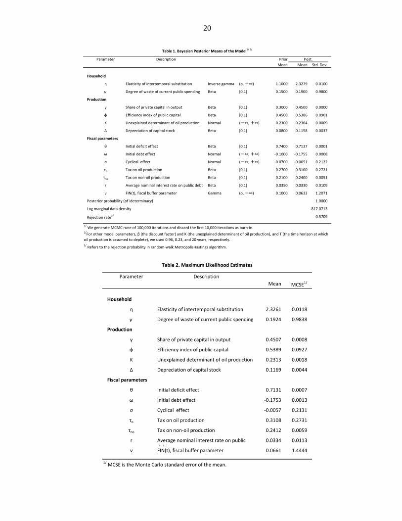
and the prior distributions. The latter, however, require some degree of judgment. Table 1

presents the priors for distributions. Most of the structural parameters of our model are based

on Cameroon-specific and past empirical studies. More specifically, the share of private

capital in output γ is the average for Cameroon, and the fiscal parameters θ (initial deficit lag

effect), ω (debt lag effect), σ (cyclical parameter), r (nominal interest rate), and τ (the tax

rates for oil and non-oil sectors) are estimated using Cameroon-specific five-year averages

(2007–11). The average tax rates on production in the oil and non-oil sectors are calculated to

be approximately 27 percent and 21 percent, respectively. The discount factor β is set at 0.96,

corresponding to the annual commercial interest rate of 4 percent currently used by the IMF

for low-income country (LIC) debt sustainability analysis. Following Takizawa, Gardner,

and Ueda (2004) for oil-producing LICs, we set the intertemporal elasticity of substitution at

1.1. On the production side, γ, the share of private capital stock in output, is set at 30 percent,

consistent with most empirical studies on LICs. The parameters ν and δ are set in line with

the recent literature on LICs (Berg and others, 2011). Following Hulten (1996), the efficiency

index of public capital φ is initially set at 0.45.35 Exogenous AR shocks to oil prices,

production, fiscal buffers (FIN), public investment, and NOPD have beta distributions for

autocorrelation coefficients with their prior mean set at 0.80. Standard errors have prior

gamma distributions, with prior mean values at 0.5 percent for oil price and production

(persistent shocks) and 0.25 percent for the others.

33 Our model specification needs to be considered against two important limitations: (i) there is no explicit

modeling of public sector congestion effects nor of a monetary sector; and (ii) we do not consider other possible

spending options and objectives of the government (for example redistributive income transfers to reduce

inequality).

34 DSGE estimates are generally considered data driven when they are obtained through maximum likelihood

techniques.

35 Hulten’s φ is an index incorporating “electricity system loss,” “road condition,” “telephone network,” and

“railway availability.” With the help of the PIMI, Dabla-Norris and others (2011) calculate an efficiency-

adjusted public capital stock and find that, for 40 LICs, only 47 percent of investment translates into productive

public capital. This is close to the 0.45 used in Hulten, even though the Hulten figure also includes the use of

productive existing capital (one can see this by substituting equation (9) into equation (5)). Pritchett (2000)

estimates that the fraction of public investment that is productive averages 0.49 for sub-Saharan African

countries. IMF (2012) cautions, however, that these are measures presumably correlated but not direct estimates

of the fraction of investment not well spent.

19

The draw from the posterior distribution was obtained by generating runs of 100,000

iterations and discarding the first 10,000 iterations as the burn-in period. Convergence of the

Markov Chain was tested by cumulated means and by using the diagnostic test developed by

Brooks and Gelman (1998). Given that DSGE models may make poor forecasts, particularly

in small-scale models like ours, even when they fit the data well; we paid attention to the

identification of some structural parameters with additional likelihood estimates.

Furthermore, caution is needed when using priors drawn from previous studies, because they

depend crucially on model specifications, assumptions, data quality, and time periods of data

analysis.

The shapes of the likelihood at the posterior mode and the Hessian condition number were

also considered to highlight the lack of identification for some parameters. Table 1 shows

there is only one structural parameter where the likelihood does not dominate the prior.

Furthermore, Canova and Sala (2009) indicate that the smaller the number of cross-equation

and cross-horizon restrictions used in estimation, the larger the chance that identification

problems will be present. However, Beltran and Draper (2008) show that more observations

help fix the identification problem and that Bayesian and likelihood estimates provide an

appropriate way to verify which parameters are poorly estimated. We then performed the

maximum likelihood estimate with numerical gradient methods and used the MCMC to

determine the posterior means of the model parameters (Table 2). The result also confirms

that only the fiscal buffer parameter appears to be weakly identified, but it exerts limited

effect on the projected endogenous variables.

20

Parameter Description Prior

Mean Mean Std. Dev.

Household

η Elasticity of intertemporal substitution Inverse gamma (ο, ＋∞) 1.1000 2.3279 0.0100

ν Degree of waste of current public spending Beta [0,1) 0.1500 0.1900 0.9800

Production

γ Share of private capital in output Beta [0,1) 0.3000 0.4500 0.0000

φ Efficiency index of public capital Beta [0,1) 0.4500 0.5386 0.0901

Κ Unexplained determinant of oil production Normal (－∞, ＋∞) 0.2300 0.2304 0.0009

Δ Depreciation of capital stock Beta [0,1) 0.0800 0.1158 0.0037

Fiscal parameters

θ Initial deficit effect Beta [0,1) 0.7400 0.7137 0.0001

ω Initial debt effect Normal (－∞, ＋∞) -0.1000 -0.1755 0.0008

σ Cyclical effect Normal (－∞, ＋∞) -0.0700 -0.0051 0.2122

τo Tax on oil production Beta [0,1) 0.2700 0.3100 0.2721

τno Tax on non-oil production Beta [0,1) 0.2100 0.2400 0.0051

r Average nominal interest rate on public debt Beta [0,1) 0.0350 0.0330 0.0109

ν FIN(t), fiscal buffer parameter Gamma (ο, ＋∞) 0.1000 0.0633 1.2071

1.0000

-817.0713

Rejection rate3/ 0.5709

1/ We generate MCMC rune of 100,000 iterations and discard the first 10,000 iterations as burn-in.

3/ Refers to the rejection probability in random-walk MetropolisHastings algorithm.

Table 1. Bayesian Posterior Means of the Model1/ 2/

2/For other model parameters, β (the discount factor) and K (the unexplained determinant of oil production), and T (the time horizon at which

oil production is assumed to deplete), we used 0.96, 0.23, and 20 years, respectively.

Post.

Posterior probability (of ideterminacy)

Log marginal data density

Parameter Description

Mean MCSE1/

Household

η Elasticity of intertemporal substitution 2.3261 0.0118

ν Degree of waste of current public spending 0.1924 0.9838

Production

γ Share of private capital in output 0.4507 0.0008

φ Efficiency index of public capital 0.5389 0.0927

Κ Unexplained determinant of oil production 0.2313 0.0018

Δ Depreciation of capital stock 0.1169 0.0044

Fiscal parameters

θ Initial deficit effect 0.7131 0.0007

ω Initial debt effect -0.1753 0.0013

σ Cyclical effect -0.0057 0.2131

τo Tax on oil production 0.3108 0.2731

τno Tax on non-oil production 0.2412 0.0059

r Average nominal interest rate on public

debt

0.0334 0.0113

ν FIN(t), fiscal buffer parameter 0.0661 1.4444

1/ MCSE is the Monte Carlo standard error of the mean.

Table 2. Maximum Likelihood Estimates

21

VI. RESULTS OF POLICY SCENARIOS

A. “Scaling-Up with Reform” Scenario

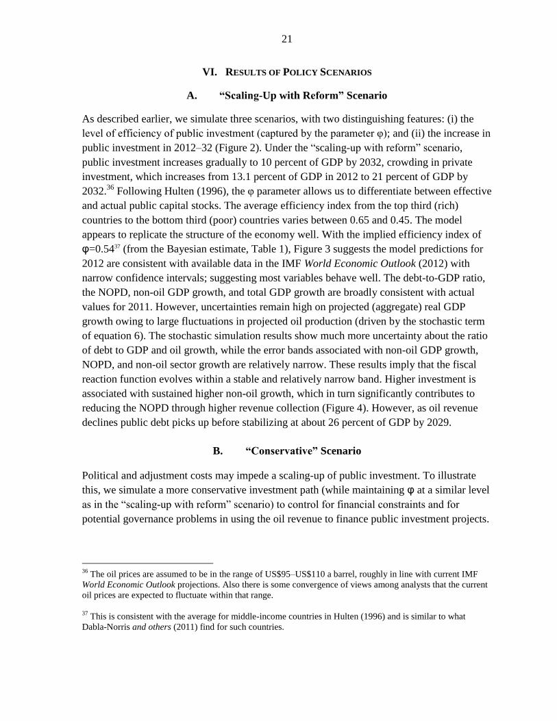
As described earlier, we simulate three scenarios, with two distinguishing features: (i) the

level of efficiency of public investment (captured by the parameter φ); and (ii) the increase in

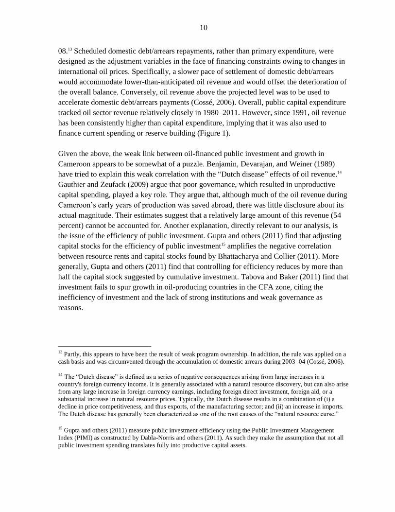
public investment in 2012–32 (Figure 2). Under the “scaling-up with reform” scenario,

public investment increases gradually to 10 percent of GDP by 2032, crowding in private

investment, which increases from 13.1 percent of GDP in 2012 to 21 percent of GDP by

2032.36

Following Hulten (1996), the φ parameter allows us to differentiate between effective

and actual public capital stocks. The average efficiency index from the top third (rich)

countries to the bottom third (poor) countries varies between 0.65 and 0.45. The model

appears to replicate the structure of the economy well. With the implied efficiency index of

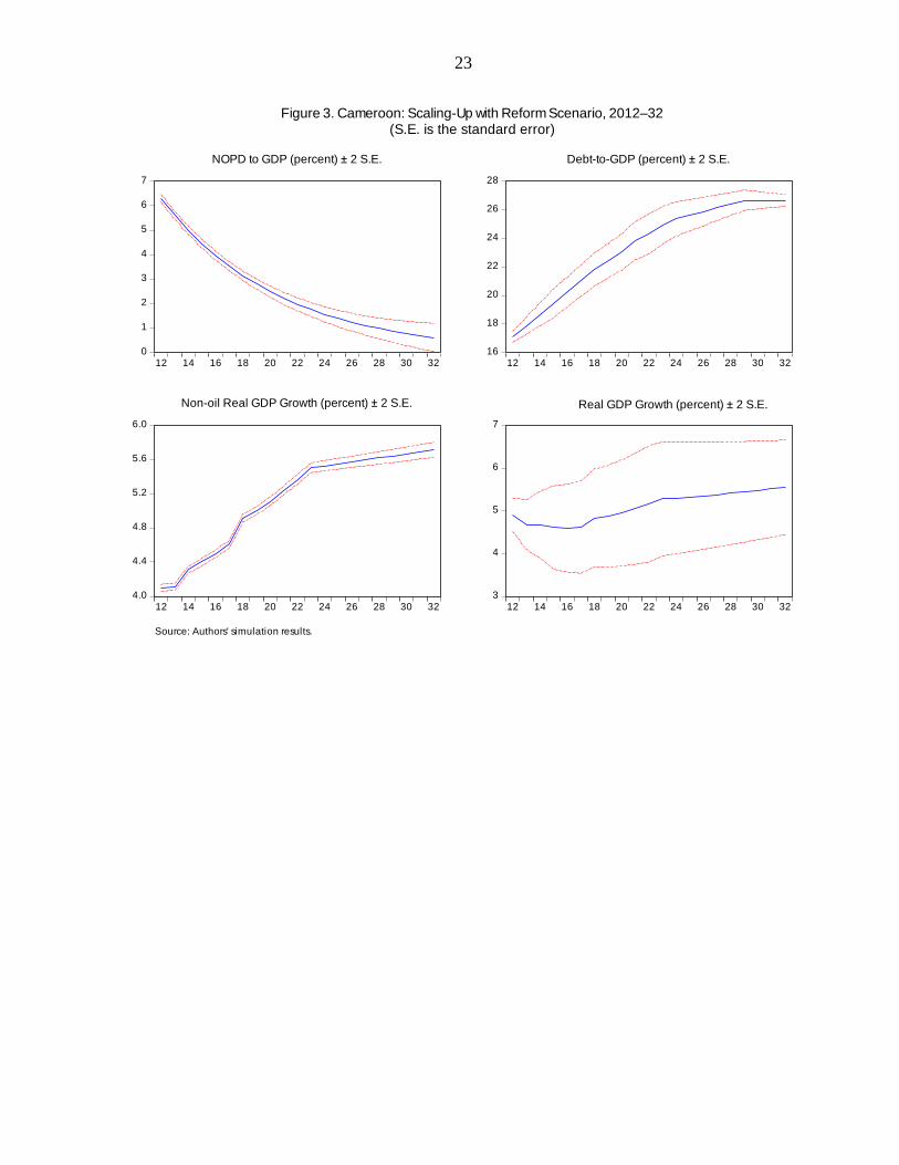
φ=0.5437 (from the Bayesian estimate, Table 1), Figure 3 suggests the model predictions for

2012 are consistent with available data in the IMF World Economic Outlook (2012) with

narrow confidence intervals; suggesting most variables behave well. The debt-to-GDP ratio,

the NOPD, non-oil GDP growth, and total GDP growth are broadly consistent with actual

values for 2011. However, uncertainties remain high on projected (aggregate) real GDP

growth owing to large fluctuations in projected oil production (driven by the stochastic term

of equation 6). The stochastic simulation results show much more uncertainty about the ratio

of debt to GDP and oil growth, while the error bands associated with non-oil GDP growth,

NOPD, and non-oil sector growth are relatively narrow. These results imply that the fiscal

reaction function evolves within a stable and relatively narrow band. Higher investment is

associated with sustained higher non-oil growth, which in turn significantly contributes to

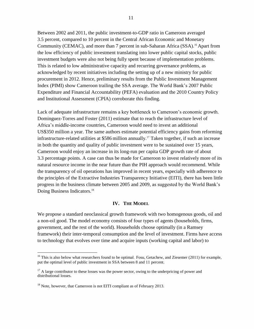
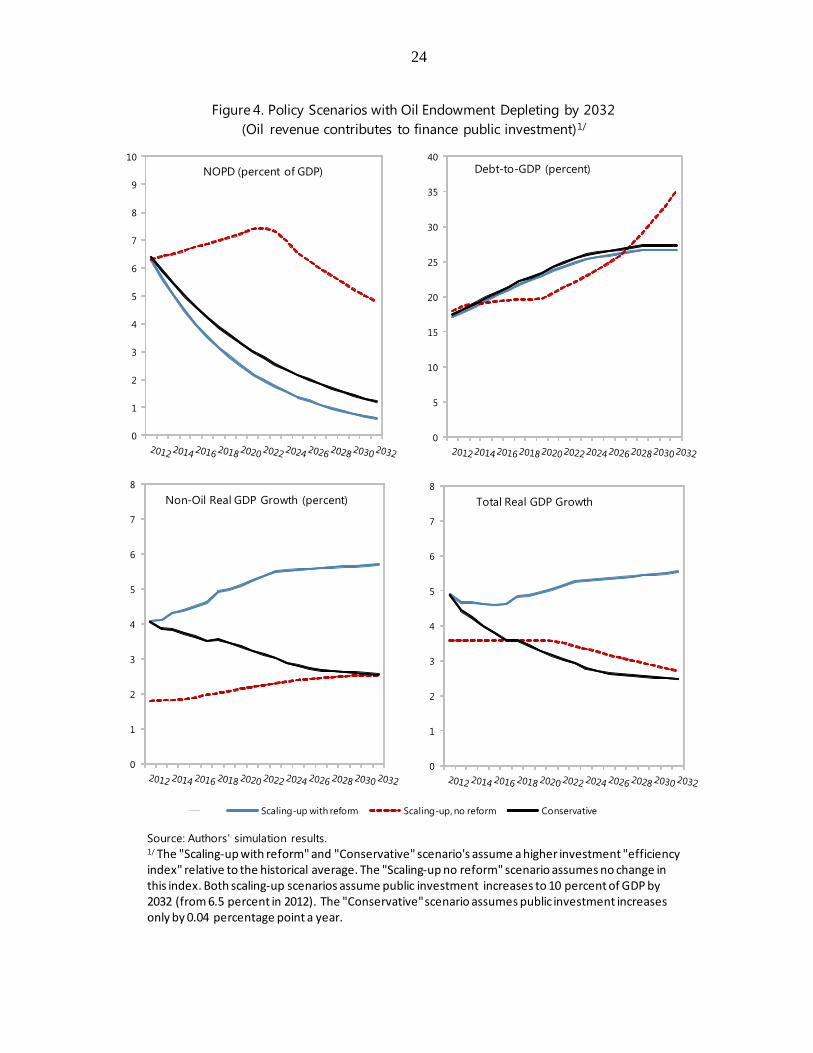
reducing the NOPD through higher revenue collection (Figure 4). However, as oil revenue

declines public debt picks up before stabilizing at about 26 percent of GDP by 2029.

B. “Conservative” Scenario

Political and adjustment costs may impede a scaling-up of public investment. To illustrate

this, we simulate a more conservative investment path (while maintaining φ at a similar level

as in the “scaling-up with reform” scenario) to control for financial constraints and for

potential governance problems in using the oil revenue to finance public investment projects.

36

The oil prices are assumed to be in the range of US$95–US$110 a barrel, roughly in line with current IMF

World Economic Outlook projections. Also there is some convergence of views among analysts that the current

oil prices are expected to fluctuate within that range.

37 This is consistent with the average for middle-income countries in Hulten (1996) and is similar to what

Dabla-Norris and others (2011) find for such countries.

22

Although improvement in the business climate and public infrastructure would be conducive

to increased private sector investment, access to (concessional) financing may prove

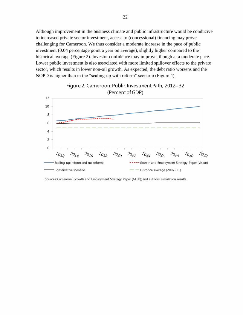
challenging for Cameroon. We thus consider a moderate increase in the pace of public

investment (0.04 percentage point a year on average), slightly higher compared to the

historical average (Figure 2). Investor confidence may improve, though at a moderate pace.

Lower public investment is also associated with more limited spillover effects to the private

sector, which results in lower non-oil growth. As expected, the debt ratio worsens and the

NOPD is higher than in the “scaling-up with reform” scenario (Figure 4).

0

2

4

6

8

10

12

Figure 2. Cameroon: Public Investment Path, 2012– 32

(Percent of GDP)

Scaling-up (reform and no-reform) Growth and Employment Strategy Paper (vision)

Conservative scenario Historical average (2007–11)

Sources: Cameroon: Growth and Employment Strategy Paper (GESP); and authors' simulation results.

23

0

1

2

3

4

5

6

7

12 14 16 18 20 22 24 26 28 30 32

NOPD to GDP (percent) ± 2 S.E.

16

18

20

22

24

26

28

12 14 16 18 20 22 24 26 28 30 32

Debt-to-GDP (percent) ± 2 S.E.

4.0

4.4

4.8

5.2

5.6

6.0

12 14 16 18 20 22 24 26 28 30 32

Non-oil Real GDP Growth (percent) ± 2 S.E.

3

4

5

6

7

12 14 16 18 20 22 24 26 28 30 32

Real GDP Growth (percent) ± 2 S.E.

Figure 3. Cameroon: Scaling-Up with Reform Scenario, 2012–32(S.E. is the standard error)

Source: Authors' simulation results.

24

Figure 4. Policy Scenarios with Oil Endowment Depleting by 2032

(Oil revenue contributes to finance public investment)1/

Source: Authors' simulation results.1/ The "Scaling-up with reform" and "Conservative" scenario's assume a higher investment "efficiency index" relative to the historical average. The "Scaling-up no reform" scenario assumes no change in this index. Both scaling-up scenarios assume public investment increases to 10 percent of GDP by 2032 (from 6.5 percent in 2012). The "Conservative"scenario assumes public investment increases only by 0.04 percentage point a year.

0

1

2

3

4

5

6

7

8

9

10

0

5

10

15

20

25

30

35

40

0

1

2

3

4

5

6

7

8

0

1

2

3

4

5

6

7

8

NOPD (percent of GDP) Debt-to-GDP (percent)

Non-Oil Real GDP Growth (percent) Total Real GDP Growth

Scaling-up with reform Scaling-up, no reform Conservative

25

Interestingly, in line with the literature on resource-rich countries, both the “scaling-up with

reform” and the “conservative” scenarios imply an early reduction of the NOPD (from an

initial large deficit, about 6.5 percent of GDP). The NOPD continuously declines while the

debt ratio is maintained at a sustainable level in 2012–32 (Figure 4). This is achieved mainly

through higher growth and stronger revenue collection. This finding is acknowledged in IMF

(2012), which notes that this issue is especially pertinent in resource-rich countries with short

reserves horizons. To some extent, concerns about long-term sustainability are reflected in

the use of the PIH approach to determine appropriate fiscal anchors for such countries.

C. “Scaling-Up No Reform” Scenario

We test a “scaling-up no reform” scenario in which no reform is undertaken to improve

governance and the effectiveness of public investment; and accordingly, there is no

crowding-in of the private sector.38 The scenario assumes the efficiency of public investment

is lower than in the other two scenarios (φ =0.45). The simulation shows that a lower

efficiency index is associated with lower non-oil GDP growth. This in turn is associated with

a higher NOPD and higher ratios of debt to GDP and debt to non-oil GDP. Consistent with

Chakraborty and Dabla-Norris (2009) and others (e.g., Esfahani and Ramirez, 2003; Hulten,

1996), this suggests that the efficiency of investment, in addition to its quantity, matters for

growth. At the given efficiency level of public investment, non-oil real growth appears to be

bound below 2.5 percent in the long run as public investment reaches 10 percent of GDP in

2032. This scenario also shows that higher public debt appears to exert a dampening effect on

growth. This finding is supported by Reinhart and Rogoff (2010).

VII. CONCLUSION AND POLICY IMPLICATIONS

In this paper we show, through a small-scale DSGE model applied to Cameroon, that a

departure from the PIH approach could be justified in the face of large investment needs. The

model features (i) exhaustible and volatile oil revenue; (ii) the impact of investment on non-

oil growth; and (iii) consideration of explicit debt dynamics and a fiscal reaction function.

Overall, our results confirm that both the size and effectiveness of public investment financed

through oil revenue matter for increasing growth in Cameroon. The effect of public

investment on growth comes through its efficiency in increasing public capital stocks. Its

complementarity with private investment appears to be the key transmission channel.

However, these results are conditional on an assumed level of efficiency, which is closer to

that observed in the average middle-income country.

38

This scenario is run to illustrate the risk of lack of progress in governance, which may make the use of natural

resource revenue insufficient to boost growth and provide better social indicators.

26

Some preliminary policy conclusions can be drawn from our simulation results for

Cameroon. With severe infrastructure bottlenecks, limited fiscal buffers, declining oil

reserves, and uncertain access to financing, a sustainable medium-term fiscal strategy that

accommodates a gradual scaling up of public investment financed through oil revenue could

be planned. Should the existing fiscal buffers not suffice, policymakers could borrow to

finance investment, provided that policy reforms are effective for enhancing the quality of

the investment. Our policy experiments underscore the importance of reforms. While the

scenario with reform provides relatively better outcomes, the scenario without reforms tends

to exert a dampening effect on growth and deteriorates fiscal performance over time. Hence,

structural reforms should feature conditions that enhance public investment efficiency and

fiscal performance (e.g., enhanced tax base and better tax collection, including user fees).

Moreover, fiscal anchors that target a medium-term debt ratio and NOPD could incorporate

sufficient flexibility to respond to uncertainty (for example, our results show that the error

bands of +/- 2 standard errors around fiscal and debt indicators are quite narrow). This is

important, given the volatility in oil prices and the need for a comfortable level of

government reserves as a buffer against exogenous shocks. Our framework is consistent with

the IMF policy advice in low-income, resource-rich countries because, by design, it is geared

to ensuring a sustainable level of non-oil production to anchor medium-and long-term

sustainability. However, these conclusions rest on the crucial assumption that issues relating

to public investment (its budgetary process and its size) and its effectiveness are addressed

swiftly to secure the growth dividends from such investment.

27

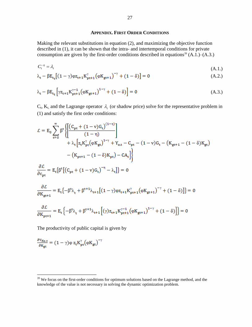
APPENDIX. FIRST ORDER CONDITIONS

Making the relevant substitutions in equation (2), and maximizing the objective function

described in (1), it can be shown that the intra- and intertemporal conditions for private

consumption are given by the first-order conditions described in equations39 (A.1.)–(A.3.)

t tC (A.1.)

(A.2.)

(A.3.)

Ct, Kt, and the Lagrange operator t (or shadow price) solve for the representative problem in

(1) and satisfy the first order conditions:

The productivity of public capital is given by

39

We focus on the first-order conditions for optimum solutions based on the Lagrange method, and the

knowledge of the value is not necessary in solving the dynamic optimization problem.

28

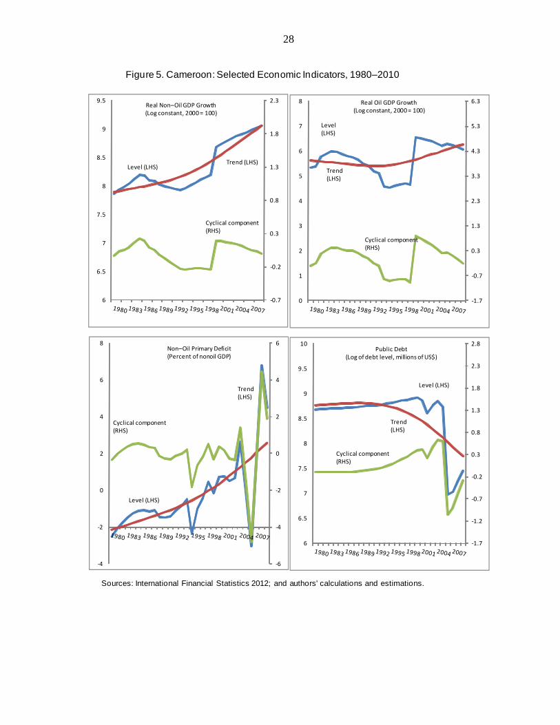
Figure 5. Cameroon: Selected Economic Indicators, 1980–2010

Sources: International Financial Statistics 2012; and authors' calculations and estimations.

-0.7

-0.2

0.3

0.8

1.3

1.8

2.3

6

6.5

7

7.5

8

8.5

9

9.5Real Non–Oil GDP Growth(Log constant, 2000 = 100)

Trend (LHS)Level (LHS)

Cyclical component(RHS)

-1.7

-0.7

0.3

1.3

2.3

3.3

4.3

5.3

6.3

0

1

2

3

4

5

6

7

8 Real Oil GDP Growth(Log constant, 2000 = 100)

Trend(LHS)

Level(LHS)

Cyclical component(RHS)

-6

-4

-2

0

2

4

6

-4

-2

0

2

4

6

8Non–Oil Primary Deficit(Percent of nonoil GDP)

Trend(LHS)

Level (LHS)

Cyclical component(RHS)

-1.7

-1.2

-0.7

-0.2

0.3

0.8

1.3

1.8

2.3

2.8

6

6.5

7

7.5

8

8.5

9

9.5

10Public Debt

(Log of debt level, millions of US$)

Trend(LHS)

Level (LHS)

Cyclical component(RHS)

29

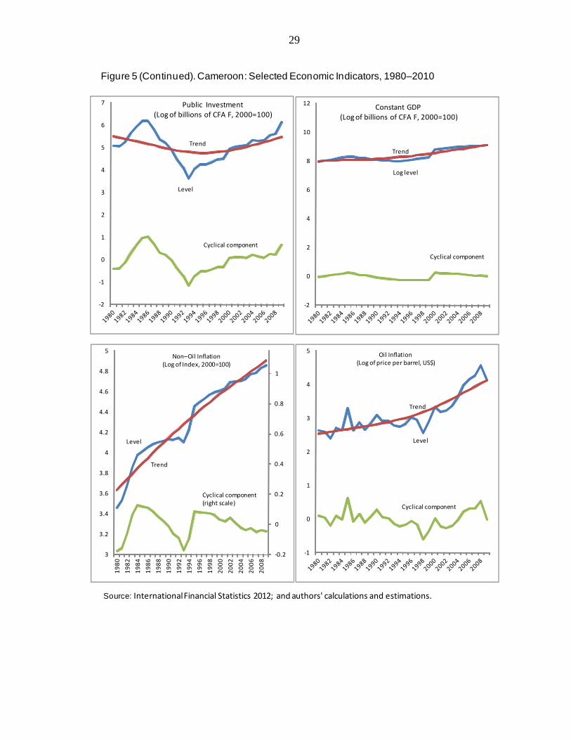
Figure 5 (Continued). Cameroon: Selected Economic Indicators, 1980–2010

Source: InternationalFinancial Statistics 2012; and authors' calculations and estimations.

-2

-1

0

1

2

3

4

5

6

7 Public Investment(Log of billions of CFA F, 2000=100)

Trend

Level

Cyclical component

-2

0

2

4

6

8

10

12Constant GDP

(Log of billions of CFA F, 2000=100)

Trend

Log level

Cyclical component

-0.2

0

0.2

0.4

0.6

0.8

1

3

3.2

3.4

3.6

3.8

4

4.2

4.4

4.6

4.8

5

19

80

19

82

19

84

19

86

19

88

19

90

19

92

19

94

19

96

19

98

20

00

20

02

20

04

20

06

20

08

Non–Oil Inflation(Log of Index, 2000=100)

Trend

Level

Cyclical component(right scale)

-1

0

1

2

3

4

5Oil Inflation

(Log of price per barrel, US$)

Trend

Level

Cyclical component

30

REFERENCES

Arbache, J., and J. Page, 2007, “More Growth or Fewer Collapses? A New Look at Long

Run Growth in Sub-Saharan Africa,” World Bank Policy Research Working Paper

No. 4384 (Washington: World Bank).

Arezki, R., A. Dupuy, and A. Gelb, 2012, “Resource Windfalls, Optimal Public Investment

and Redistribution: The Role of Total Factor Productivity and Administrative

Capacity,” IMF Working Paper 12/200 (Washington: International Monetary Fund).

Barnett, S., and R. Ossowski, 2003, “Operational Aspects of Fiscal Policy in Oil-Producing

Countries,” in Fiscal Policy Formulation and Implementation in Oil-Producing

Countries, ed. by Jeffrey Davis, Rolando Ossowski, and Annalisa Fedelino

(Washington: International Monetary Fund).

Barro, R. J., 1990, “Government Spending in a Simple Model of Endogenous Growth,”

Journal of Political Economy, Vol. 98 (October, Part 2), pp. S103–25.

Baunsgaard, T., M. Villafuerte, M. Poplawski-Ribeiro, and C. Richmond, 2012, “Fiscal

Frameworks for Resource Rich Developing Countries,” Staff Discussion Note 12/04

(Washington: International Monetary Fund).

Beltran, O. D., and D. Draper, 2008, “Estimating the Parameters of a Small Open

Economy DSGE Model: Identifiability and Inferential Validity,” Board of Governors

of the Federal Reserve System, International Finance Discussion Papers, No. 955,

November 2008.

Benjamin, N., S. Devarajan, and R.J. Weiner, 1989, “Dutch Disease in a Developing

Country: Oil Reserves in Cameroon,” Journal of Development Economics, Vol. 30

(January), pp. 71–92.

Berg, A., R. Portillo, S. S. Yang, and L.F. Zanna, 2013, “Public Investment in Resource-

Abundant Developing Countries,” IMF Economic Review, advance online

publication, April 2.

Bhattacharya, S., and P. Collier, 2011, “Public Capital in Resource Rich Economies: Is There

a Curse?” CSAE Working Paper No. 2011−14 (Oxford: Center for the Study of

African Economies).

31

Bjerkholt, O., and I. Niculescu, 2004, “Fiscal Rules for Economies with Nonrenewable

Resources: Norway and Venezuela,” in Rules-Based Fiscal Policy in Emerging

Markets: Background, Analysis and Prospects, ed. by G. Kopits (New York:

Palgrave, MacMillian).

Brooks, S., and A. Gelman, 1998, “General Methods for Monitoring Convergence of

Iterative Simulations,” Journal of Computational and Graphical Statistics, 7,

pp. 434−455.

Canova, F. and L. Sala, 2009, “Back to square one: Identification issues in DSGE models,”

Journal of Monetary Economics, Elsevier, vol. 56(4), pp. 431-449.

Chakraborty, S., and E. Dabla-Norris, 2009, “The Quality of Public Investment,” IMF

Working Paper No. 09/154 (Washington: International Monetary Fund).

Collier, P., R. Van der Ploeg, M. Spence, and A. J. Venables, 2010, “Managing Resource

Revenues in Developing Countries,” Staff Papers, International Monetary Fund,

Vol. 57, No. 1.

Cossé, S., 2006, “Strengthening Transparency in the Oil Sector in Cameroon: Why Does It

Matter?” IMF Policy Discussion Paper 06/2 (Washington: International Monetary

Fund).

Dabla-Norris, E., J. Brumby, A. Kyobe, Z. Mills, and C. Papageogiou, 2011, “Investing in

Public Investment: An Index of Public Investment Efficiency,” IMF Working Paper

11/37 (Washington: International Monetary Fund).

Dominguez-Torres, C., and V. Foster, 2011, “Cameroon’s Infrastructure: A Continental

Perspective,” World Bank Policy Research Working Paper No. 5822 (Washington:

World Bank).

Essama-Nssah, B., and L. Bassolé, 2010, “A Counterfactual Analysis of the Poverty Impact

of Economic Growth in Cameroon,” World Bank Policy Research Working Paper

5249 (Washington: World Bank).

Esfahani, H., and M. Ramirez, 2003, “Institutions, Infrastructure, and Economic Growth,”

Journal of Development Economics, Vol. 70, pp. 443–477.

Finn, M.G., 1998, ‘‘Cyclical Effects of Government’s Employment and Goods Purchases,’’

International Economic Review 39, pp. 635---657.

32

Fosu, A., Y. Getachew, and T. Ziesemer, 2011, “Optimal Public Investment, Growth, and

Consumption: Evidence from African Countries,” CSAE Working Paper 2011−22

(Oxford, U.K.: Centre for the Study of African Economies, Oxford University).

Gali, J., and R. Perotti , 2003, ‘‘Fiscal Policy and Monetary Integration in Europe,’’ NBER

Working Paper 9773 (Cambridge: National Bureau of Economic Research).

Gauthier, B., and A. Zeufack, 2009, “Governance and Oil Revenue in Cameroon,” OxCarre

Research Paper 38, Department of Economics, University of Oxford.

Gelb, A., and S. Grasmann, 2010, “How Should Oil Exporters Spend their Rents,” Center for

Global Development Working Paper 221 (Washington: Center for Global

Development).

Gupta, S., A. Kangur, C. Papageorgiou, and A. Wane, 2011, “Efficiency Adjusted Public

Capital and Growth,” IMF Working Paper 11/217 (Washington: International

Monetary Fund).

Government of Cameroon, 2009, “Growth and Employment Strategy Paper,” accessed via

www.imf.org/external/pubs/ft/scr/2010/cr10257.pdf.

Harding, T., and R. Van der Ploeg, 2009, “Is Norway's Bird-in-Hand Stabilization Fund

Prudent Enough? Fiscal Reactions to Hydrocarbon Windfalls and Graying

Populations,” CESifo Working Paper Series 2830 (Munich: CESifo Group).

Hulten, C., 1996, “Infrastructure Capital and Economic Growth: How Well You Use It May

Be More Important than How Much You Have,” NBER Working Paper 5847

(Cambridge, Massachusetts: National Bureau of Economic Research).

Husted, S., 1992, “The Emerging US Current Account Deficit in the 1980s: a Cointegration

Analysis,” The Review of Economics and Statistics 74, pp. 159–166.

International Monetary Fund, 2007, “Cameroon: Selected Issues,” www.imf.org,

(Washington: International Monetary Fund).

International Monetary Fund, 2010, “How Countercyclical and Pro-Poor Has Fiscal Policy

Been During the Downturn?” Regional Economic Outlook: Sub-Saharan Africa,

April (Washington: International Monetary Fund).

International Monetary Fund, 2012, “Macroeconomic Policy Frameworks for Resource-Rich

Developing Countries,” www.imf.org, (Washington: International Monetary Fund).

33

Iossifov, P., K. Noriaki, M. Takebe, R. York, and Z. Zhan, 2009, “Improving Surveillance

across the CEMAC Region,” IMF Working Paper 09/260 (Washington: International

Monetary Fund).

Katz, M., U. Bartsch, H. Malhotra, and M. Cuc, 2004, Lifting the Oil Curse: Improving

Petroleum Revenue Management in Sub-Saharan Africa (Washington: International

Monetary Fund).

Pattichis, C., 2010, “The Intertemporal Budget Constraint and Current Account Sustainability

in Cyprus: Evidence and Policy Implications,” Applied Economics, 42, 04 pp. 463–

473.

Pritchett, L., 2000, “The Tyranny of Concepts: CUDIE (Cumulated, Depreciated, Investment

Effort) Is Not Capital,” Journal of Economic Growth, Vol.5, pp. 361–84.

Ramsey, F., 1928, “A Mathematical Theory of Saving,” Economic Journal, Vol. 38, pp. 543–

559.

Reinhart, C. M., and K.S. Rogoff, 2010, “Growth in a Time of Debt,” American Economic

Review, 100(2): pp. 573–78.

Segura, A., 2006, “Management of Oil Wealth under the Permanent Income Hypothesis: The

Case of São Tomé and Principe,” IMF Working Paper 06/183 (Washington:

International Monetary Fund).

Tabova, A., and C. Baker, 2011, “Determinants of Non-oil Growth in the CFA-

Zone Oil Producing Countries: How do they Differ?” IMF Working Paper 11/233

(Washington: International Monetary Fund).

Takizawa, H., E.H. Gardner, and K. Ueda, 2004, “Are Developing Countries

Better Off Spending Their Oil Wealth Upfront?” IMF Working Paper 04/141

(Washington: International Monetary Fund).

Talvi, E., and C. Végh, 2005, “Tax Base Variability and Procyclicality of Fiscal Policy,”

Journal of Development Economics, 78(1):pp. 156–190.

34

Van der Ploeg, R., 2012, “Bottlenecks in Ramping Up Public Investment,” OxCarre

Research Paper 66 (Oxford, U.K.: Oxford Centre for the Analysis of Resource Rich

Economies, Oxford University).

Van der Ploeg, R., and A. J. Venables, 2011, “Harnessing Windfall Revenues: Optimal

Policies for Resource-Rich Developing Countries,” Economic Journal, Vol. 121,

pp. 1–30.