Firm Level Productivity, Risk, and Return∗

Ayse Imrohoroglu† Selale Tüzel‡

January 2013

Abstract

This paper provides new evidence about the link between firm level total factor productivity(TFP) and stock returns. We estimate firm level TFP and show that it is strongly relatedto several firm characteristics such as size, the book to market ratio, investment, and hiringrate. Low productivity firms earn a significant premium over high productivity firms in thefollowing year, and this premium is countercyclical. We show that a production based assetpricing model calibrated to match the cross section of measured firm level TFPs can replicatethe empirical relationship between TFP, many firm characteristics, and stock returns. Ourresults offer an explanation as to how these firm characteristics rationally predict returns.

JEL classification: D2, E23, E32, E44, G12

Keywords: Firm Level Productivity, Cross Section of Returns

∗We thank the seminar participants at USC, UCLA, University of Hawaii, University of Minnesota, UT Dallas,Ozyegin University, Federal Reserve Bank of New York, Early Career Women in Finance Conference, Koç FinanceConference, CASEE Conference at ASU, Vienna Macroeconomics Workshop, Canadian Macroeconomics AnnualMeeting, the 2011 Western Finance Association Meetings, and the 2011 meetings of the Society for EconomicDynamics for their comments.†Department of Finance and Business Economics, Marshall School of Business, University of Southern Cali-

fornia, Los Angeles, CA 90089-1427. E-mail: ayse@marshall.usc.edu‡Department of Finance and Business Economics, Marshall School of Business, University of Southern Cali-

fornia, Los Angeles, CA 90089-1427. E-mail: tuzel@marshall.usc.edu.

Vast evidence exists that total factor productivity (TFP) is an important determinant of eco-

nomic fluctuations, economic growth, and per capita income differences across countries. Quan-

tifying the effi ciency with which inputs utilized in production are turned into output, TFP is

also an important determinant of a firm’s value added.1 It provides a broader gauge of firm

level performance than some of the more conventional measures, such as labor productivity or

firm profitability.2

There is reason to expect TFP to be a predictor of excess firm returns. A growing strand

of literature has introduced equilibrium models that tie differences in firm characteristics and

returns to the optimal decisions of firms in response to changes in productivity and discount

rates.3 In these models, low productivity firms turn out to be more vulnerable to business

cycles, and end up being riskier than firms with high productivity. However, none of these

papers has estimated firm level productivity and investigated this fundamental relationship.

In this paper, we attempt to fill this gap by estimating firm level TFP and providing new

evidence about the sources of return predictability. We document that our measured TFP

is strongly related to several firm characteristics, such as size, the book to market ratio, in-

vestment, and hiring rate. Empirical research in finance has documented that many of these

characteristics forecast future stock returns.4 We find that TFP is positively and monotoni-

cally related to contemporaneous monthly stock returns and negatively related to future excess

returns and ex-ante discount rates. We show that a production based asset pricing model cal-

ibrated to match the cross section of measured firm level TFPs can replicate the empirical

relationships between TFP, many firm characteristics, and stock returns fairly well. Overall,

our results provide an explanation as to why these firm characteristics rationally predict returns.

1 In corporate finance, similar TFP measures are utilized in studies such as Schoar (2002); Kovenock andPhillips (1997); and McGuckin and Nguyen (1995).

2Profitability captures only the part of the value added that goes to shareholders, and labor productivity canbe an inadequate measure of overall effi ciency especially in capital intensive industries. See Lieberman and Kang(2008) for a case study of a Korean steelmaker for the differences between TFP and profitability in measuringfirm performance.

3Some of the papers in this literature include Gomes, Kogan, and Zhang (2003); Zhang (2005); Gourio (2007);Bazdresch, Belo, and Lin (2010); Li, Livdan, and Zhang (2009); Tüzel (2010); Belo and Lin (2012); and Jonesand Tüzel (Forthcoming).

4These findings are documented in Fama and French (1992); Titman, Wei, and Xie (2003); Lyandres, Sun,and Zhang (2008); Cooper, Gulen, and Schill (2008); Bazdresch, Belo, and Lin (2010); Wu, Zhang, and Zhang(2010), Belo and Lin (2010); and Tüzel (2010). Many other papers document that firm characteristics are relatedto average stock returns including Ball (1978); Banz (1981); Basu (1983); De Bondt and Thaler (1985); Bhandari(1988); Jegadeesh and Titman (1993); Chan, Jegadeesh, and Lakonishok (1996); Sloan (1996); and Thomas andZhang (2002).

1

We estimate firm level productivity using the semi-parametric method initiated by Olley

and Pakes (1996) and construct a panel of TFP levels for publicly traded firms in the U.S. We

establish a set of stylized facts by examining the summary statistics of firms sorted by TFP into

ten portfolios between 1963 and 2009. We find that differences in measured firm level TFPs are

strongly related to differences in a number of firm characteristics. High TFP firms are typically

growth firms with an average book to market ratio of about 0.5, and low TFP firms are value

firms with an average book to market ratio of about 1.4. We find the relationship between firm

size and TFP to be similarly monotonic across deciles. The average size of the firms in the

lowest TFP decile is 19% of the average firm size, whereas the size of firms in the highest TFP

decile is 372% of the average size. In addition, the hiring rate, fixed investment to capital ratio,

asset growth, profitability, and inventory growth are all monotonically increasing in firm level

TFP.

We find that low productivity firms on average earn a 7.7% annual premium in excess

returns over high productivity firms in the following year. We also find that there is significant

variation in the TFP premium over business cycles. The return spread is about three times as

high during economic contractions as it is during expansions. We interpret the spread in the

average returns across these portfolios as the risk premia associated with the higher risk of low

productivity firms. A Fama-MacBeth regression of monthly stock returns on lagged firm level

TFP produces a negative and statistically significant average slope for TFP. Quantitatively, our

regression results indicate about 7.5% higher expected returns for the firms in the lowest TFP

decile compared to a firm in the highest TFP decile.

In addition to realized returns, we also look at ex-ante measures of discount rates. Specif-

ically, we examine implied cost of capital measures calculated using three different methods,

namely those of Gebhardt, Lee, and Swaminathan (2001); Hou, van Dijk, and Zhang (2012);

and Wu and Zhang (2012). The advantage of using an implied cost of capital is that it does

not rely on realized returns that are often noisy and may be a bad proxy for expected returns.

We confirm the negative relationship between firm productivity and expected returns, finding

that the average implied cost of capital for the low TFP portfolio exceeds that of the high TFP

portfolio and is statistically significant. Similar to average future returns, the spread in implied

cost of capital is also strongly countercyclical.

In an attempt to understand the mechanism behind the negative relationship between the

2

firms’TFP and expected returns, we investigate whether there are systematic differences in

the sensitivity of low and high TFP firms’operating performance to aggregate shocks in the

economy. We find that the profits of low TFP firms are more sensitive to aggregate shocks

than are those of high TFP firms. Furthermore, the sensitivity of low TFP firms increases in

recessions, whereas the opposite happens for the high TFP firms. These results provide direct

evidence on the higher risk of low TFP firms, especially in recessions, rather than indirect

evidence based on realized or ex-ante returns.

The parameters of the TFP process are an important input in production based asset pricing

models focused on firm characteristics. We estimate the persistence of firm level TFP to be

0.7 and the standard deviation of the TFP shock to be 0.27, both at the annual frequency.

Our estimates are roughly in line with the parameters used in this literature, in which firm

level TFP processes are typically calibrated to match the moments of some key variables.5 Our

findings can serve as a direct measurement of the firm level TFP process to guide future work.

To interpret our empirical findings, we use a production-based asset pricing model similar

to those in Zhang (2005); Bazdresch, Belo, and Lin (2010); and Jones and Tüzel (Forthcoming).

We calibrate the model to the TFP moments we estimate and find that it can replicate the

empirical relationship between TFP, firm characteristics, and stock returns.

In the model economy, firms are ex-ante identical but diverge over time due to idiosyncratic

shocks. Firms that receive repeated bad shocks end up being low TFP firms. These firms are

characterized by low investment and hiring rates, high B/M ratios, and smaller size relative to

the industry average. Firms that receive multiple good shocks become high TFP firms with

high investment and hiring rates, low B/M ratios, and large market capitalizations.

In this framework, a negative relationship between a firm’s productivity and its level of

risk arises endogenously due to the presence of frictions in adjusting capital. All firms face

aggregate shocks and incur adjustment costs upon changes in the capital stock. In recessions

(low aggregate productivity), most firms try to scale back their production and lower their

investments and hiring. Even though all firms suffer during a recession, the firms that suffer

the most are those with low firm level TFP. If the recession deepens, these firms have the most

pressure to scale back their investments and hence suffer the most from convex adjustment

costs, resulting in low firm values and low returns. This is especially important in the presence

5For example, see Zhang (2005), Gomes (2001), and Hennessy and Whited (2005).

3

of a countercyclical price of risk, which is introduced through an exogenous pricing kernel.

During recessions, the returns of low productivity firms fluctuate more closely with aggregate

productivity, and those firms become particularly risky. The opposite happens in expansions.

Our simulation results indicate that differences in firm level TFPs can indeed generate

realistic differences in firm characteristics and stock returns. In particular, the model can

replicate reasonably well the investment to capital ratio, hiring rate, book to market ratio, size,

and returns of low versus high TFP firms and their variation over the business cycle observed

in the data.

Section 1 summarizes the data and our empirical results. Section 2 presents the model and

the numerical results for the calibrated economy. Section 3 concludes. The Appendix provides

detailed information on the data, estimation of firm level productivities, and sensitivity results.

1 Empirical Results

We start this section by summarizing the data and the estimation of TFP. Next, we examine the

relationship between firm level TFP and many firm characteristics and investigate the extent to

which productivity, an economic fundamental, is linked to the cross sectional dispersion in firm

characteristics. Subsequently, we document the relationship between TFP and stock returns

using several different methods, which leads to our hypothesis that low TFP firms are riskier

than high TFP firms. Finally, we investigate how the profitability of firms change in response

to aggregate shocks conditional on their TFPs and the current state of the economy.

1.1 Data

The key variables for estimating the firm level productivity are the firm level value added,

employment, and capital. We use firm level data from Compustat and supplement it with

output and investment deflators from the Bureau of Economic Analysis and wage data from

the Social Security Administration. The sample is an unbalanced panel with approximately

12,750 distinct firms spanning the years between 1962 and 2009. Following Fama and French

(1992), we start our sample in 1962 since Compustat data for earlier years have a serious

selection bias. Estimation of TFPs requires at least two years of data, so our TFP estimates

4

start in 1963. Some of the key variables are firm level capital stock (kit) given by gross Plant,

Property, and Equipment (PPEGT)6, deflated following Hall (1990), and the stock of labor

(lit) given by the number of employees (EMP), both from Compustat. We compute firm level

value added using Compustat data on sales, operating income, and employees; we then deflate

it using the output deflator.

Monthly stock returns are from the Center for Research in Security Prices (CRSP). We

measure the contemporaneous returns over the same horizon as TFPs, matching year t TFPs to

returns from January of year t to December of year t. In predictability regressions (calculating

the future returns), to ensure that accounting information is already impounded into stock

prices, we match CRSP stock return data from July of year t to June of year t + 1 with

accounting information for fiscal year ending in year t− 1, as in Fama and French (1992, 1993),

allowing for a minimum of a six month gap between fiscal year-end and return tests. In other

words, we match the productivities calculated using accounting data for the fiscal year ending

in year t− 1 (spanning 1963 to 2009) to stock returns from July of year t to June of year t+ 1

(from July 1964 to June 2011). Similar to Fama and French (1993), our sample includes firms

with ordinary common equity as classified by CRSP, excluding ADRs, REITs, and units of

beneficial interest, and in order to avoid the survival bias in the data, we include firms in our

sample after they have appeared in Compustat for two years. Detailed information about the

data is provided in the Appendix.

1.2 TFP

Total factor productivity is a measure of the overall effectiveness with which capital and labor

are used in a production process. We estimate the production function given in:

yit = β0 + βkkit + βllit + ωit + ηit (1)

where yit is the log of value added for firm i in period t. lit, kit are log values of labor, and

capital of the firm. ωit is the productivity, and ηit is an error term not known by the firm or

the econometrician. We employ the semi-parametric procedure suggested by Olley and Pakes

6 In our estimation, we use the book value of capital, rather than proxy the market value of capital from thevalue of the firm. The market value of the firm includes the firm’s growth options, which are unrelated to thefirm’s current output and inputs. See Philippon (2009).

5

(1996) to estimate the parameters of this production function, which is explained in detail

in the Appendix. The major advantage of this approach over more traditional estimation

techniques such as the ordinary least squares (OLS) is its ability to control for selection and

simultaneity biases and deal with the within firm serial correlation in productivity that plagues

many production function estimates.7

Once we estimate the production function parameters (βo, βl, and βk), we obtain the firm

level (log) TFPs by:

ωit = yit − βo − βllit − βkkit. (2)

In the estimation, we use industry specific time dummies. Hence, our firm TFPs are free of the

effect of industry or aggregate TFP in any given year.

The production function parameters are estimated every year using all data available up

until that year to mitigate a potential look-ahead bias in the TFP estimates. We compute

TFPs for each year using that year’s data and the corresponding production function estimates

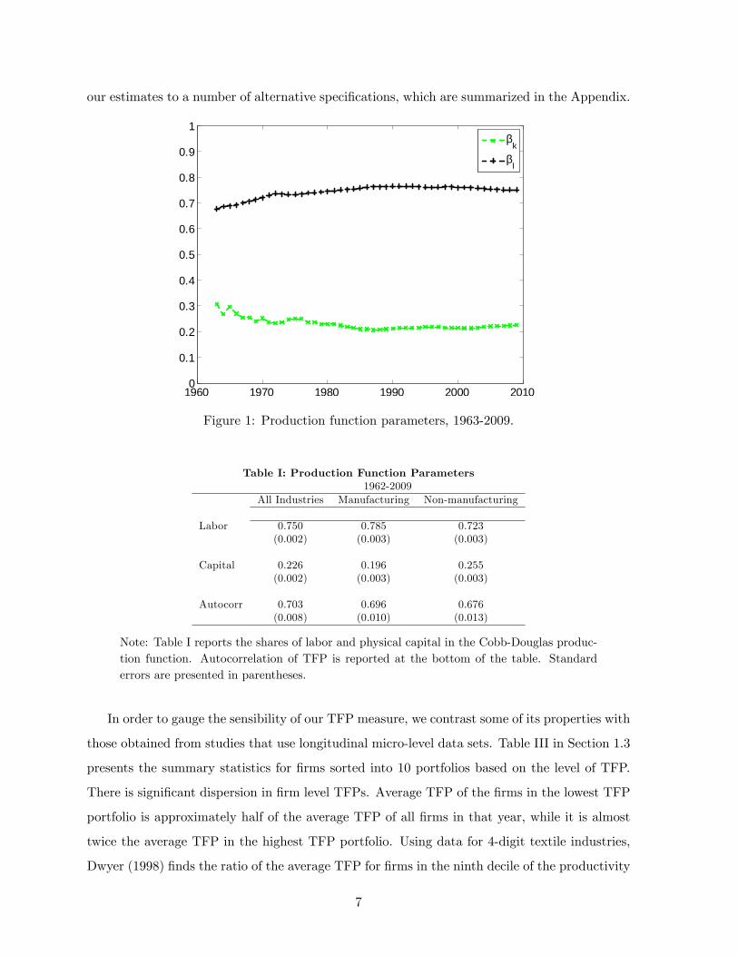
for that year. Figure 1 plots the production function estimates used in the TFP calculations.

The estimates for βl and βk are quite stable over the years: βl ranges from 0.68 to 0.76, and

βk ranges from 0.21 to 0.31. Since the estimations use progressively more data over the years,

most of the variation in estimates occur in the earlier years. Table I tabulates the estimates for

the production function parameters and their standard errors using the entire sample period for

manufacturing and non-manufacturing firms. The results for all the firms combined, presented

in column two, indicate a labor share of 0.75 and a capital share of 0.23. The estimates for

the persistence and conditional volatility of TFP are 0.70 and 0.27, respectively, at the annual

frequency.8 As in the time series results, production function estimates are fairly similar for the

manufacturing and non-manufacturing sectors. Having stable production function estimates

over time and for different industries is reassuring since it contributes to the robustness of our

asset pricing results to different specifications and data samples. We check the sensitivity of

7The static OLS production function estimates reveal that within firm residuals, which are the productivityestimates in that setting, are serially correlated. The simultaneity bias arises if the firm’s factor input decisionis influenced by the TFP that is observed by the firm. This means that the regressors and the error term in anOLS regression are correlated. The selection bias in the OLS regressions arises due to firms exiting the sampleused in estimating the production function parameters. If the exit probability is correlated with productivity,not accounting for the selection issue may bias the parameter estimates.

8The conditional volatility of TFP is computed from the persistence and the cross sectional standard devia-tion of firm productivity as 0.27

(= 0.38×

√1− 0.72

). The cross sectional dispersion of firm level productivity

increases from 0.23 in 1963 to 0.53 in 2009. We take the cross sectional standard deviation to be 0.375, which isthe average dispersion over this time period.

6

our estimates to a number of alternative specifications, which are summarized in the Appendix.

1960 1970 1980 1990 2000 20100

0.1

0.2

0.3

0.4

0.5

0.6

0.7

0.8

0.9

1β

k

βl

Figure 1: Production function parameters, 1963-2009.

Table I: Production Function Parameters1962-2009

All Industries Manufacturing Non-manufacturing

Labor 0.750 0.785 0.723(0.002) (0.003) (0.003)

Capital 0.226 0.196 0.255(0.002) (0.003) (0.003)

Autocorr 0.703 0.696 0.676(0.008) (0.010) (0.013)

Note: Table I reports the shares of labor and physical capital in the Cobb-Douglas produc-tion function. Autocorrelation of TFP is reported at the bottom of the table. Standarderrors are presented in parentheses.

In order to gauge the sensibility of our TFP measure, we contrast some of its properties with

those obtained from studies that use longitudinal micro-level data sets. Table III in Section 1.3

presents the summary statistics for firms sorted into 10 portfolios based on the level of TFP.

There is significant dispersion in firm level TFPs. Average TFP of the firms in the lowest TFP

portfolio is approximately half of the average TFP of all firms in that year, while it is almost

twice the average TFP in the highest TFP portfolio. Using data for 4-digit textile industries,

Dwyer (1998) finds the ratio of the average TFP for firms in the ninth decile of the productivity

7

distribution relative to the average in the second decile to be between 2 and 4 at the plant level.

Similar findings are reported in Olley and Pakes (1996) for the telecommunications equipment

industry and in Syverson (2004) for four-digit manufacturing industries. For our sample, which

consists of TFPs at the firm level rather than plant level, this measure is 1.8. These comparisons

provide some confirmation that the dispersion in TFPs obtained in our sample is consistent with

plant level evidence presented earlier.

Next, we examine the evolution of the productivity by constructing the transition probability

matrix, which shows the probability of a plant/firm moving from a certain productivity decile in

a period to other deciles in the next period. Table II presents the transition probability matrix

for the firms in our sample sorted into decile TFP portfolios. The probabilities of staying in the

lowest or the highest TFP portfolios are about 50%. The higher probabilities along the diagonal

shows that there is some persistence in productivity. These results are similar to the findings

reported in Bartelsman and Dhrymes (1998) who examine the transition probabilities of plant

level TFPs in three industries over the 1972-1986 period. They report that about 50-70% of

the plants in the lowest and highest deciles tend to stay in the same bin for all three industries.

Table II also reports the probability that a firm in a given portfolio will disappear from

our sample in the next year. The drop-off may be the result of either firm failure or a missing

data item in the following year. The probability of drop-off ranges from 8-9% for the firms

in the higher TFP portfolios to 16% for the firms in the lowest TFP portfolio. The negative

relationship between drop-off rates and TFP shows that low productivity firms are more likely

to disappear from our sample where the difference in the drop-off rates can be interpreted as

the higher likelihood of failure for low TFP firms.

Table II: Portfolio Transition Probabilities

Year tTFP Low 2 3 4 5 6 7 8 9 High Drop-offLow 0.45 0.19 0.07 0.04 0.02 0.02 0.02 0.01 0.01 0.01 0.162 0.18 0.32 0.19 0.09 0.05 0.03 0.02 0.01 0.01 0.00 0.123 0.08 0.18 0.26 0.18 0.09 0.05 0.03 0.02 0.01 0.00 0.114 0.05 0.09 0.18 0.23 0.17 0.10 0.05 0.03 0.01 0.00 0.10

Year 5 0.03 0.05 0.10 0.18 0.23 0.17 0.09 0.04 0.02 0.01 0.09t− 1 6 0.02 0.03 0.05 0.10 0.18 0.23 0.17 0.08 0.03 0.01 0.09

7 0.02 0.02 0.03 0.05 0.10 0.18 0.25 0.18 0.07 0.02 0.088 0.02 0.02 0.02 0.03 0.05 0.09 0.19 0.29 0.18 0.04 0.089 0.02 0.01 0.02 0.02 0.02 0.04 0.08 0.20 0.37 0.14 0.09

High 0.02 0.01 0.01 0.01 0.01 0.02 0.02 0.04 0.17 0.61 0.09

Note: Table II reports the transition probability matrix for the firms sorted into decile TFP

8

portfolios.

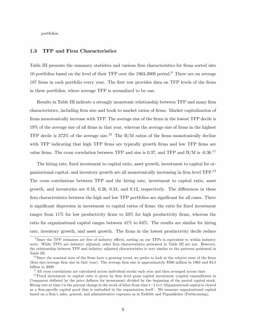
1.3 TFP and Firm Characteristics

Table III presents the summary statistics and various firm characteristics for firms sorted into

10 portfolios based on the level of their TFP over the 1963-2009 period.9 There are on average

187 firms in each portfolio every year. The first row provides data on TFP levels of the firms

in these portfolios, where average TFP is normalized to be one.

Results in Table III indicate a strongly monotonic relationship between TFP and many firm

characteristics, including firm size and book to market ratios of firms. Market capitalization of

firms monotonically increase with TFP. The average size of the firms in the lowest TFP decile is

19% of the average size of all firms in that year, whereas the average size of firms in the highest

TFP decile is 372% of the average size.10 The B/M ratios of the firms monotonically decline

with TFP indicating that high TFP firms are typically growth firms and low TFP firms are

value firms. The cross correlation between TFP and size is 0.37, and TFP and B/M is -0.36.11

The hiring rate, fixed investment to capital ratio, asset growth, investment to capital for or-

ganizational capital, and inventory growth are all monotonically increasing in firm level TFP.12

The cross correlations between TFP and the hiring rate, investment to capital ratio, asset

growth, and inventories are 0.16, 0.26, 0.24, and 0.12, respectively. The differences in these

firm characteristics between the high and low TFP portfolios are significant for all cases. There

is significant dispersion in investment to capital ratios of firms; the ratio for fixed investment

ranges from 11% for low productivity firms to 33% for high productivity firms, whereas the

ratio for organizational capital ranges between 41% to 64%. The results are similar for hiring

rate, inventory growth, and asset growth. The firms in the lowest productivity decile reduce

9Since the TFP estimates are free of industry effects, sorting on our TFPs is equivalent to within industrysorts. While TFPs are industry adjusted, other firm characteristics presented in Table III are not. However,the relationship between TFP and industry adjusted characteristics is very similar to the patterns presented inTable III.10Since the nominal sizes of the firms have a growing trend, we prefer to look at the relative sizes of the firms

(firm size/average firm size in that year). The average firm size is approximately $500 million in 1963 and $4.5billion in 2009.11All cross correlations are calculated across individual stocks each year and then averaged across time.12Fixed investment to capital ratio is given by firm level gross capital investment (capital expenditures in

Compustat deflated by the price deflator for investment) divided by the beginning of the period capital stock.Hiring rate at time t is the percent change in the stock of labor from time t−1 to t. Organizational capital is viewedas a firm-specific capital good that is embodied in the organization itself . We measure organizational capitalbased on a firm’s sales, general, and administrative expenses as in Eisfeldt and Papanikolau (Forthcoming).

9

their workforce by around 3% and their assets shrink on average 1%, whereas firms in the

highest productivity decile increase their workforce by 21% and experience 36% asset growth.

Inventory growth varies between 5% and 36%. The ratio of research and development expense

(R&D) to the property, plant, and equipment (PPE) of the firm also tends to increase with

TFP, but the relationship is not perfectly monotonic.13 Table III also shows that the real estate

ratio of low productivity firms exceed the average in their industry whereas the real estate ratio

of high productivity firms is lower than their industry average. The relationship between the

average age (computed as the number of years since the firm first shows up in Compustat) and

TFP is inverse U-shaped.

Many of the relationships we document here are consistent with the predictions of production-

based asset pricing models used in Zhang (2005) to explain the value premium; in Bazdresch,

Belo, and Lin (2010) for investment and hiring behavior; in Jones and Tüzel (Forthcoming) and

Belo and Lin (2012) for inventory investment; and Tüzel (2010) for real estate ratio. In these

economies, ex-ante identical firms become heterogeneous due to firm level TFP shocks. Firms

that receive repeated bad shocks end up being small firms with low investment and hiring rates,

and high B/M ratios. Firms that receive multiple good shocks become high TFP firms with

high investment and hiring rates, low B/M ratio, and end up being large firms. In Section 2,

our simulation results indicate that differences in firm level TFPs estimated from the data can

indeed generate differences in firm characteristics similar to the ones found in Table III.

We also investigate the relationship between firm TFP and measures of profitability. Pro-

ductivity and profitability have often been used interchangeably in finance literature (for exam-

ple, Novy-Marx (Forthcoming) and Gourio (2007)) where unobserved productivity is frequently

proxied by measures of profitability.14 We look at three profitability measures. Our first mea-

sure is the return on equity (ROE), which is the profitability measure used in Fama and French

(2008) and calculated as Net income available to common stockholders/Book equity. The sec-

ond profitability measure is the return on assets (ROA), defined as Net income/Total assets.

13The data item for R&D expense is not populated for all firms. R&D expense can also be considered as atype of investment; however, taking R&D as a seperate capital item would lead to the exclusion of a significantpart of our sample. In untabulated results, we find that constructing a capital stock from R&D expense usingthe perpetual inventory method and adding that capital stock to the fixed capital leads to similar results.14Even though productivity and profitability are expected to be related, their calculation and interpretation

are different. Profits can be interpreted as the rents to capital owners (which are the owners of the firm), whereasproductivity is a measure of how effi cient the firm is in converting inputs (labor and capital) to outputs (valueadded).

10

Our last profitability measure is Gross profits/Book assets from Novy-Marx (Forthcoming),

which we label “gross”profitability (GPR). All three measures of profitability are monotoni-

cally and positively related to TFP. The cross correlation of TFP with GPR is quite modest

(0.18), whereas its correlations with ROE and ROA are higher (0.48 and 0.61, respectively).15

We report additional firm characteristics that are found to be related to future stock returns.

Net stock issues (net shares) are on average negative for all portfolios but are particularly low

for high TFP firms. Also, TFP is negatively related to leverage, with the least productive firms

possessing the highest leverage.

Table III: Descriptive Statistics for TFP Sorted Portfolios, 1963-2009

Low 2 3 4 5 6 7 8 9 High High-Low

TFP 0.51 0.70 0.79 0.85 0.91 0.96 1.03 1.12 1.26 1.86 1.35

SIZE 0.19 0.27 0.39 0.52 0.68 0.89 1.30 1.65 2.28 3.72 3.53(21.87)

B/M 1.38 1.34 1.20 1.07 0.96 0.86 0.76 0.68 0.59 0.51 -0.87(-13.38)

I/K 0.11 0.09 0.10 0.11 0.13 0.14 0.16 0.18 0.22 0.33 0.22(19.09)

AG -0.01 0.05 0.08 0.11 0.13 0.15 0.18 0.21 0.26 0.36 0.36(13.72)

HR -0.03 0.01 0.03 0.05 0.07 0.09 0.12 0.12 0.19 0.21 0.25(13.27)

INV 0.05 0.08 0.10 0.12 0.13 0.16 0.21 0.23 0.34 0.36 0.31(12.24)

IOC/OC 0.41 0.36 0.37 0.38 0.40 0.41 0.44 0.47 0.54 0.64 0.23(14.73)

RD/PPE 0.12 0.06 0.06 0.05 0.05 0.05 0.06 0.08 0.11 0.20 0.08(8.18)

RER (*10) 0.02 0.05 0.06 0.06 0.02 0.06 0.01 -0.02 -0.05 -0.13 -0.15(-3.95)

NS -0.08 -0.06 -0.06 -0.06 -0.07 -0.07 -0.07 -0.07 -0.10 -0.14 -0.06(-5.55)

LEV 0.27 0.29 0.28 0.27 0.25 0.23 0.20 0.18 0.15 0.12 -0.15(-11.49)

ROE -0.21 -0.05 0.01 0.04 0.07 0.09 0.10 0.12 0.14 0.17 0.37(27.01)

ROA -0.07 0.00 0.02 0.04 0.05 0.06 0.07 0.08 0.09 0.11 0.18(25.86)

GPR 0.34 0.39 0.41 0.43 0.44 0.46 0.46 0.47 0.48 0.50 0.16(15.00)

AGE 14.55 16.66 16.96 17.25 17.39 17.30 17.01 16.50 15.31 13.67 -0.89(-3.91)

Note: For each variable, averages are first taken over all firms in that portfolio, then overyears. On average, there are 187 firms in each portfolio every year. Average TFP each yearis normalized to be 1. SIZE is the market capitalization of firms in June of year t + 1.

15We investigate the relationship between TFP, profitability and investments further in section 1.4.2.

11

Average size each year is normalized to 1. B/M is the ratio of book equity for the lastfiscal year-end in year t divided by market equity in December of year t. I/K is the fixedinvestment to capital ratio. AG is the change in the natural log of assets, HR is the changein the natural log of number of employees, and INV is the change in the natural log oftotal inventories, all measured from year t− 1 to year t. Ioc/OC is the ratio of investmentin organization capital to the stock of organization capital in year t, both computed fromthe deflated sales, general and administrative expenses. RD/PPE is the ratio of researchand development expenses to gross PPE in year t. RER is the ratio of buildings +capitalleases to PPE in year t , adjusted for industries. NS is the change in the natural log of thesplit-adjusted shares outstanding from the fiscal year-end in t− 1 to t. LEV is the ratio oflong-term debt holdings in year t to the firm’s total assets calculated as the sum of theirlong-term debt and the market value of their equity in December of year t. ROE is thenet income in year t divided by book equity for year t. ROA is the net income in year tdivided by total assets for year t. GPR is the gross profits in year t divided by book assetsfor year t. AGE is computed in year t as the number of years since the firm first shows upin Compustat. N is the average number of firms in each portfolio in year t.

1.4 Asset Pricing Implications

1.4.1 Returns of TFP-sorted portfolios

In Table IV, we investigate the relationship between our firm level TFPs and the contempo-

raneous and future annualized excess returns (excess of the risk free rate). The table presents

both equal and value weighted portfolio returns for firms sorted into 10 portfolios based on

the level of TFP in year t. Our results show that TFP is positively and monotonically related

to contemporaneous stock returns. The difference between the returns of high and low TFP

firms is 24.8% for equal-weighted portfolios and 17.0% for value-weighted portfolios, and both

spreads are statistically significant.16 The relationship between the level of TFP and future

excess returns is equally striking for equal-weighted portfolios: low productivity firms on av-

erage earn a 7.7% annual premium over high productivity firms in the following year, and the

return spread is statistically significant. The unconditional return spread is lower (1.3%) and

not significant for the value-weighted portfolios.

In order to understand the relationship between TFP and future returns over the business

cycles, we separate our sample into expansionary and contractionary periods around the port-

folio formation time. We use industrial production as our business cycle variable. Industrial

16 In untabulated results, we find even a stronger relationship between the innovations in TFP and contempo-raneous stock returns. When we sort firms based on innovations in TFP, the spread in returns is 42% for theequal-weighted and 22% for the value-weighted portfolios.

12

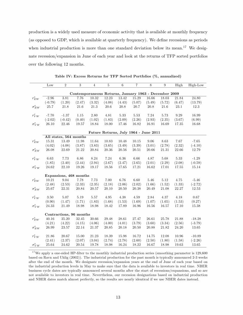
production is a widely used measure of economic activity that is available at monthly frequency

(as opposed to GDP, which is available at quarterly frequency). We define recessions as periods

when industrial production is more than one standard deviation below its mean.17 We desig-

nate recession/expansion in June of each year and look at the returns of TFP sorted portfolios

over the following 12 months.

Table IV: Excess Returns for TFP Sorted Portfolios (%, annualized)

Low 2 3 4 5 6 7 8 9 High High-Low

Contemporaneous Returns, January 1963 - December 2009reEW -2.96 3.81 7.76 10.32 12.23 13.42 15.29 16.66 18.03 21.84 24.80

(-0.79) (1.20) (2.47) (3.32) (4.08) (4.43) (5.07) (5.49) (5.72) (6.47) (13.79)σeEW 25.7 21.8 21.6 21.3 20.6 20.8 20.7 20.8 21.6 23.1 12.3

reVW -7.70 -1.37 1.15 2.80 4.81 5.33 5.53 7.24 5.73 9.29 16.99(-2.02) (-0.42) (0.40) (1.02) (1.83) (2.09) (2.26) (2.93) (2.35) (3.67) (6.99)

σeVW 26.10 22.46 19.57 18.84 18.00 17.46 16.82 16.91 16.69 17.35 16.68

Future Returns, July 1964 - June 2011All states, 564 months

reEW 15.31 13.49 11.98 11.64 10.83 10.48 10.15 9.06 8.63 7.67 -7.65(4.02) (4.08) (3.87) (3.83) (3.65) (3.49) (3.39) (3.01) (2.78) (2.32) (-4.10)

σeEW 26.08 22.69 21.22 20.84 20.36 20.56 20.51 20.66 21.31 22.66 12.79

reVW 6.63 7.73 6.86 8.24 7.24 6.36 6.66 4.87 5.68 5.33 -1.29(1.85) (2.40) (2.44) (2.94) (2.67) (2.47) (2.65) (2.01) (2.29) (2.08) (-0.59)

σeVW 24.62 22.10 19.26 19.17 18.56 17.65 17.21 16.62 17.01 17.55 15.14

Expansions, 468 monthsreEW 10.21 9.04 7.78 7.73 7.00 6.76 6.60 5.46 5.12 4.75 -5.46

(2.48) (2.53) (2.33) (2.35) (2.18) (2.06) (2.02) (1.66) (1.52) (1.33) (-2.72)σeEW 25.67 22.31 20.84 20.57 20.10 20.50 20.38 20.49 21.08 22.27 12.53

reVW 3.50 5.07 5.19 5.57 4.95 4.38 4.59 2.84 4.37 4.18 0.67(0.90) (1.47) (1.71) (1.83) (1.68) (1.53) (1.69) (1.07) (1.65) (1.53) (0.27)

σeVW 24.33 21.49 18.98 18.98 18.42 17.89 16.96 16.56 16.57 17.10 15.38

Contractions, 96 monthsreEW 40.16 35.20 32.45 30.66 29.48 28.61 27.47 26.61 25.78 21.88 -18.28

(4.21) (4.22) (4.15) (4.06) (4.00) (4.01) (3.79) (3.60) (3.34) (2.56) (-3.79)σeEW 26.99 23.57 22.14 21.37 20.85 20.18 20.50 20.88 21.82 24.20 13.65

reVW 21.86 20.67 15.00 21.23 18.39 15.98 16.72 14.75 12.08 10.96 -10.89(2.41) (2.37) (2.07) (3.04) (2.74) (2.78) (2.60) (2.50) (1.80) (1.58) (-2.26)

σeVW 25.64 24.62 20.54 19.78 18.98 16.24 18.22 16.67 18.98 19.63 13.65

17We apply a one-sided HP-filter to the monthly industrial production series (smoothing parameter is 129,600based on Ravn and Uhlig (2002)). The industrial production for the past month is typically announced 2-3 weeksafter the end of the month. We designate recession/expansion years at the end of June of each year based onthe industrial production levels in May to make sure that the data is available to investors in real time. NBERbusiness cycle dates are typically announced several months after the start of recessions/expansions, and so arenot available to investors in real time. Nevertheless, our recession designations based on industrial productionand NBER dates match almost perfectly, so the results are nearly identical if we use NBER dates instead.

13

Note: reEW is equal-weighted monthly excess returns (excess of risk free rate). reV W is value-weighted monthly excess returns, annualized, averages are taken over time (%). σeEW andσeV W are the corresponding standard deviations. Contemporaneous returns are measuredin the year of the portfolio formation, from January of year t to December of year t. Futurereturns are measured in the year following the portfolio formation, from July of year t+ 1to June of year t+ 2 and annualized (%). t− statistics are in parentheses. Expansion andcontraction periods are designated in June of year t+ 1 based on the level of (one sidedHP-filtered) industrial production in May of that year. Returns over the expansions andcontractions are measured from July of year t+ 1 to June of year t+ 2.

We find that the negative relationship between TFP and expected returns persists both

in expansions and in contractions for equal-weighted portfolios. However, there are significant

differences in returns over the business cycles. The average level of expected returns is much

higher in recessions, approximately 30%, than expansions, 7%. The spread between the returns

of high and low TFP portfolios are also much higher during contractions, 18.3%, than expan-

sions, 5.5%, in equal weighted portfolios. For value-weighted portfolios, the spread is 11% and

is significant over contractions. During expansions, however, the spread is not significant.

Even though all portfolios have higher expected returns in recessions, the increase in ex-

pected returns of low TFP portfolios is roughly twice as much as it is for the high TFP portfolios.

We interpret the spread in the average returns across these portfolios, especially in recessions,

as the risk premia associated with the higher risk of low productivity firms.

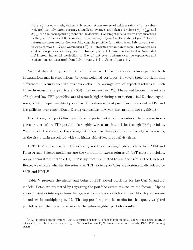
In Table V we investigate whether widely used asset pricing models such as the CAPM and

Fama-French 3-factor model capture the variation in excess returns of TFP sorted portfolios.

As we demonstrate in Table III, TFP is significantly related to size and B/M at the firm level.

Hence, we explore whether the returns of TFP sorted portfolios are systematically related to

SMB and HML.18

Table V presents the alphas and betas of TFP sorted portfolios for the CAPM and FF

models. Betas are estimated by regressing the portfolio excess returns on the factors. Alphas

are estimated as intercepts from the regressions of excess portfolio returns. Monthly alphas are

annualized by multiplying by 12. The top panel reports the results for the equally-weighted

portfolios, and the lower panel reports the value-weighted portfolio results.

18MKT is excess market returns; SMB is returns of portfolio that is long in small, short in big firms; HML isreturns of portfolio that is long in high B/M, short in low B/M firms. (Fama and French, 1992, 1993, amongothers)

14

Table V: Alphas and Betas of Portfolios Sorted on TFP (%, annualized)Dependent Variable: Excess Returns, July 1964 - June 2011

Low 2 3 4 5 6 7 8 9 High High-Low

Equal-weighted Portfolios

CAPM

alpha 8.86 7.52 6.17 5.79 5.04 4.54 4.11 2.92 2.28 0.88 -7.99(3.50) (3.75) (3.55) (3.59) (3.32) (3.10) (3.03) (2.21) (1.70) (0.63) (-4.27)

MKT 1.24 1.15 1.11 1.12 1.11 1.14 1.16 1.18 1.22 1.30 0.07(26.79) (31.32) (35.16) (38.19) (40.16) (42.77) (46.93) (49.15) (49.97) (51.21) (1.93)

FF

alpha 4.37 2.60 1.67 1.25 0.87 0.79 1.13 0.30 0.28 -0.02 -4.39(2.62) (2.09) (1.61) (1.42) (0.99) (0.89) (1.34) (0.35) (0.32) (-0.02) (-2.74)

MKT 1.02 1.02 1.01 1.03 1.03 1.05 1.06 1.08 1.09 1.14 0.12(31.33) (42.25) (49.95) (60.46) (60.20) (60.49) (64.34) (63.86) (63.34) (63.30) (3.79)

HML 0.27 0.46 0.44 0.47 0.43 0.37 0.24 0.19 0.08 -0.12 -0.39(5.56) (12.70) (14.38) (18.10) (16.63) (13.96) (9.83) (7.66) (2.94) (-4.48) (-8.38)

SMB 1.27 1.01 0.88 0.84 0.77 0.73 0.69 0.66 0.67 0.66 -0.61(27.89) (29.98) (31.19) (35.16) (32.16) (29.99) (30.15) (27.78) (27.77) (26.40) (-13.87)

Value-weighted Portfolios

CAPM

alpha -0.19 1.20 1.16 2.39 1.65 0.92 1.33 -0.34 0.40 -0.09 0.10(-0.10) (0.83) (0.93) (2.21) (1.48) (0.99) (1.52) (-0.43) (0.47) (-0.10) (0.05)

MKT 1.31 1.25 1.09 1.12 1.07 1.04 1.02 1.00 1.01 1.04 -0.27(36.60) (47.34) (47.94) (56.80) (53.09) (61.42) (63.92) (70.89) (65.41) (63.12) (-6.91)

FF

alpha -1.53 -0.60 -0.57 0.50 -0.13 0.23 0.91 -0.22 1.44 1.82 3.35(-0.88) (-0.43) (-0.47) (0.51) (-0.12) (0.24) (1.02) (-0.28) (1.77) (2.25) (1.87)

MKT 1.17 1.23 1.10 1.12 1.11 1.07 1.04 1.01 1.03 1.02 -0.15(34.66) (45.45) (46.76) (57.59) (54.49) (59.04) (60.73) (66.17) (64.93) (64.58) (-4.30)

HML -0.03 0.21 0.23 0.24 0.29 0.13 0.09 0.00 -0.11 -0.28 -0.26(-0.57) (5.11) (6.45) (8.22) (9.36) (4.70) (3.35) (0.02) (-4.81) (-11.97) (-4.85)

SMB 0.63 0.28 0.20 0.24 0.08 0.00 -0.02 -0.05 -0.17 -0.15 -0.78(13.46) (7.30) (6.13) (8.87) (2.78) (-0.19) (-0.94) (-2.32) (-7.84) (-6.73) (-16.03)

Note: The table presents the regressions of equal-weighted and value-weighted excess port-folio returns on various factor returns. MKT, SMB, and HML factors are taken from KenFrench’s website. The portfolios are sorted on TFP. Alphas are annualized (%). Returnsare measured from July 1964 to June 2011. t−statistics are calculated by dividing the slopecoeffi cient by its time series standard error and presented in parentheses.

We find that low TFP portfolios load heavily on SMB, whereas the loadings of the high TFP

portfolios are low, even negative in some cases. The loadings on HML are non-monotonic, but

15

higher TFP portfolios have lower loadings than lower TFP portfolios. The equal-weighted port-

folios have a non-monotonic loading on MKT, whereas the value-weighted low TFP portfolios

have significantly higher loading on MKT compared to the high TFP portfolios. Neither the

CAPM, nor the FF 3-factor model completely explain the return spread in the equally weighted

portfolios: High-Low TFP portfolio has a CAPM alpha around —8%, and FF alpha of -4.5%,

which are both statistically significant. The spreads in alphas of value-weighted portfolios are

positive but not statistically significant.19

Our takeaway from these results is not necessarily that TFP is a separate risk factor that

is not captured by these factors but rather that TFP is systematically related to SMB, and to

some extent to HML, which we further investigate empirically and through a model economy.

1.4.2 Fama-MacBeth Regressions

In Section 1.4.1, we examine the characteristics and realized average returns of portfolios sorted

on TFP. In this section, we run Fama-MacBeth cross-sectional regressions (Fama and MacBeth,

1973) of monthly stock returns on lagged firm level TFP as well as other control variables.

The estimates of the slope coeffi cients in Fama-MacBeth regressions allow us to determine the

magnitude of the effect of the firm characteristics on excess stock returns.

Table VI reports the time series averages of cross-sectional regression slope coeffi cients

and their time-series t-statistic (computed as in Newey-West with 4 lags) obtained from the

Fama-MacBeth regressions. In all specifications, the dependent variable is the excess monthly

stock returns, annualized to make the magnitudes comparable to the results in Table IV. The

first specification in Table VI shows the relationship between the level of TFP and future

excess returns. The cross sectional regression, where log TFP is the only explanatory variable,

produces a negative and statistically significant average slope. The magnitude of the effect

is significant as well. The −5.66 average regression coeffi cient in this setting translates into

approximately 7.5% higher expected returns for the firms in the lowest TFP decile compared

to a firm in the highest TFP decile.

19 In an untabulated, extended specification, we include two other commonly used factors, Carhart’s momentumfactor (MOM) and Pastor and Stambaugh’s liquidity factor (LIQ). Pastor and Stambaugh (2003) document astrong relationship between size and liquidity, so higher returns of low TFP firms (which are typically smaller)could potentially be explained by their exposure to the liquidity factor. We find that MOM and LIQ factors arenot systematically related to the returns of the TFP sorted portfolios, and the results are very similar to that ofthe FF model.

16

Table VI: Fama-MacBeth Regressions with Other Predictors (%, annualized)July 1964 - June 2011

Int TFP BM SIZE I/K HR INV AG ROE ROA GPR NS RER LEV RD/PPE AGE

I 10.6 -5.7(3.0) (-3.6)

II 11.8 -1.0 4.5(3.4) (-0.8) (5.0)

III 7.0 -1.8 -1.9(2.3) (-1.6) (-4.1)

IV 11.8 -4.4 -8.0(3.6) (-2.6) (-3.3)

V 11.0 -4.9 -3.7(3.2) (-3.0) (-4.2)

VI 10.9 -5.2 -2.0(3.2) (-3.1) (-3.5)

VII 11.6 -3.9 -5.5(3.4) (-2.4) (-4.9)

VIII 10.8 -4.3 -4.9(3.0) (-3.3) (-2.1)

IX 11.8 -2.7 -22.2(3.0) (-2.1) (-1.9)

X 5.9 -6.2 5.9(3.4) (-4.0) (3.4)

XI 10.5 -5.6 -1.2(3.1) (-3.6) (-1.5)

XII 11.9 -6.0 1.0(3.2) (-3.2) (0.5)

XIII 8.6 -4.2 7.5(2.7) (-3.1) (2.3)

XIV 10.3 -6.0 6.9(3.1) (-3.8) (1.5)

XV 12.1 -5.8 -0.1(2.8) (-3.7) (-1.4)

Note: The table presents the average slopes and their t−statistics from monthly cross-section regressions to predict excess stock returns. Results are reported for the wholesample period of July 1964 to June 2011. The t−statistics for the average regression slopesuse the time-series standard deviations of the monthly slopes (computed as in Newey-Westwith 4 lags) and presented in parentheses. Excess returns are predicted for July of yeart + 1 to June of t + 2. Average TFP each year is normalized to be 1. SIZE is the logmarket capitalization of firms in June of year t+ 1. Average size each year is normalized to1. B/M is the ratio of book equity for the last fiscal year-end in year t divided by marketequity in December of year t. I/K is the fixed investment to capital ratio, AG is the changein the natural log of assets, HR is the change in the natural log of number of employees,and INV is the change in the natural log of total inventories, all measured from year t− 1to year t. NS is the change in the natural log of the split-adjusted shares outstanding fromthe fiscal year-end in t − 1 to t. LEV is the ratio of long-term debt holdings in year t to

17

the firm’s total assets calculated as the sum of their long-term debt and the market value oftheir equity in December of year t. RER is the ratio of buildings+capital leases to PPE inyear t , adjusted for industries. ROE is the net income in year t divided by book equityfor year t. ROA is the net income in year t divided by total assets for year t. GPR is thegross profits in year t divided by book assets for year t. RD/PPE is the ratio of research anddevelopment expenses to gross PPE in year t. AGE is computed in year t as the number ofyears since the firm first shows up in Compustat. Excess returns are annualized (%).

In specifications II-XV, we examine the marginal predictive power of TFP after controlling

for several firm level characteristics that are known to predict stock returns and/or found to

systematically vary with TFP in Table III.

Specification II considers firm’s B/M, III considers size, IV considers investment to capital

ratio, V considers hiring rate, VI considers inventory growth, and VII considers asset growth.

Specifications VIII through X consider different measures of profitability: ROE in VIII, ROA

in IX, and gross profitability in specification X. We study net share issues in XI, real estate

ratio in XII, leverage in XIII, R&D/PPE in XIV, and firm age in XV. The definitions of these

variables are available in Appendix, Section 4.2. We observe that the cross sectional regressions

in specifications I to XV produce negative and statistically significant average slopes for TFP

except for the specifications in II and III where including book to market (in II) and size (in

III) erodes the significance of TFP.

The results of these predictability regressions should be interpreted with caution, however.

In production based asset pricing models, shocks to firm level productivity create ex-post dif-

ferences across firms in terms of the level of TFP, which affect the riskiness of a stock and its

future expected returns. The same shock is the fundamental variable that drives the differences

in size, B/M, and many other firm characteristics across firms. To the extent that such models

correctly describe firm behavior, characteristics such as size, B/M, and investment/capital ratio

should not have additional explanatory power vis-a-vis productivity but should be determined

by it. Furthermore, even if firm productivity is the fundamental variable that drives firm be-

havior, it is arguably measured with more noise than characteristics such as size or B/M, which

are observable rather than estimated. As a result, in return predictability regressions which

include both firm productivity and other firm characteristics as forecasting variables, the better

measured variables are expected to drive out productivity. Our overall goal is to shed some

light on why firm characteristics can rationally predict returns and not necessarily to come up

with a variable that outperforms other firm characteristics in return predictability regressions.

18

TFP, Expected Profitability, and Expected Investment The results of the Fama-

MacBeth regressions, similar to our earlier results based on portfolio sorts, demonstrate that

high TFP firms have lower future returns. In section 1.3 we also document that TFP is related

to many other variables, in particular, several variables related to firm investments (such as

I/K, asset growth, inventory investment) and profits (ROE, ROA, gross profitability), that are

known to predict returns. Specifically, we find that TFP is positively related to both firm in-

vestments and profitability. Thus our results are somewhat surprising, given that the literature

has documented negative relationship between investments and future returns, but generally

positive relationship between profitability and future returns.

Fama and French (2006) uses the basic valuation equation to demonstrate the basic rela-

tionship between the market/book value of the equity, expected future profitability, expected

future investments, and expected returns:20

Mt

Bt=∞∑τ=1

E(Yt+τBt− ∆Bt+τ

Bt

)(1 + r)τ

(3)

whereMt and Bt are the market and book value of equity, respectively, and Yt is the equity earn-

ings per share. The predictions that come out of the valuation equation about the link between

expected returns, r, expected investments, Et(∆Bt+τBt

), and expected profitability, Et(Yt+τBt

)are: (1) Controlling for the M/B, and expected profitability, firms with high expected invest-

ment (and asset growth) have low expected stock returns. (2) Controlling for the M/B, and

expected asset growth, firms with high expected profitability have high expected stock returns.

Therefore, expected profitability and expected investment are related to expected returns with

the opposite sign after controlling for the remaining two variables. Proxying for expected fu-

ture profitability and investments with current profitability and investments, Fama and French

(2006) have confirmed these relationships in the data.21

Table VII investigates how TFP is related to future profitability and asset growth in equation

3.22 We find that TFP strongly predicts both future profitability and future asset growth for

several years. The slope coeffi cient estimates imply that profitability and asset growth of firms

20Recently, Hou, Xue and Zhang (2012) derive similar relationships using a simple two-period investment basedasset pricing model.21Novy-Marx (Forthcoming) and Hou, Xue and Zhang (2012) report similar findings.22We scale firm profits by total assets, rather than book equity, to be able to compare the slope coeffi cients

from two regressions.

19

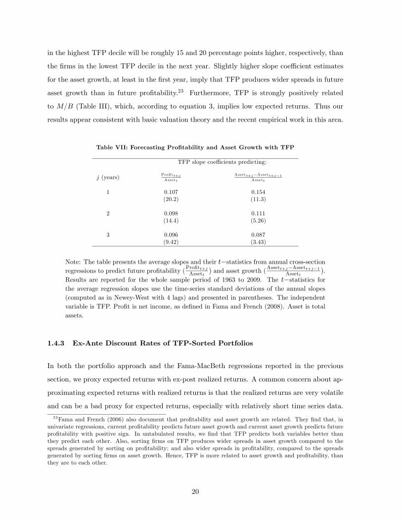
in the highest TFP decile will be roughly 15 and 20 percentage points higher, respectively, than

the firms in the lowest TFP decile in the next year. Slightly higher slope coeffi cient estimates

for the asset growth, at least in the first year, imply that TFP produces wider spreads in future

asset growth than in future profitability.23 Furthermore, TFP is strongly positively related

to M/B (Table III), which, according to equation 3, implies low expected returns. Thus our

results appear consistent with basic valuation theory and the recent empirical work in this area.

Table VII: Forecasting Profitability and Asset Growth with TFP

TFP slope coeffi cients predicting:

j (years) Profitt+jAssett

Assett+j−Assett+j−1Assett

1 0.107 0.154(20.2) (11.3)

2 0.098 0.111(14.4) (5.26)

3 0.096 0.087(9.42) (3.43)

Note: The table presents the average slopes and their t−statistics from annual cross-sectionregressions to predict future profitability (

Profitt+jAssett

) and asset growth (Assett+j−Assett+j−1Assett).

Results are reported for the whole sample period of 1963 to 2009. The t−statistics forthe average regression slopes use the time-series standard deviations of the annual slopes(computed as in Newey-West with 4 lags) and presented in parentheses. The independentvariable is TFP. Profit is net income, as defined in Fama and French (2008). Asset is totalassets.

1.4.3 Ex-Ante Discount Rates of TFP-Sorted Portfolios

In both the portfolio approach and the Fama-MacBeth regressions reported in the previous

section, we proxy expected returns with ex-post realized returns. A common concern about ap-

proximating expected returns with realized returns is that the realized returns are very volatile

and can be a bad proxy for expected returns, especially with relatively short time series data.

23Fama and French (2006) also document that profitability and asset growth are related. They find that, inunivariate regressions, current profitability predicts future asset growth and current asset growth predicts futureprofitability with positive sign. In untabulated results, we find that TFP predicts both variables better thanthey predict each other. Also, sorting firms on TFP produces wider spreads in asset growth compared to thespreads generated by sorting on profitability; and also wider spreads in profitability, compared to the spreadsgenerated by sorting firms on asset growth. Hence, TFP is more related to asset growth and profitability, thanthey are to each other.

20

To address this concern, we use an ex-ante measure of the discount rates, the implied cost of

capital, and examine its cross-sectional relationship with TFP.

The implied cost of capital (ICC) of a given firm is the internal rate of return that equates

the firm’s stock price to the present value of expected future cash flows (earnings forecasts).

Most ICC estimates in the literature, such as Gebhardt, Lee, and Swaminathan (GLS, 2001),

rely on analyst forecasts of future earnings. However, analyst forecasts are not available in the

first few years of our sample period. Furthermore, analysts tend to follow larger and more visible

stocks, so earnings forecasts of many firms in our sample are not available. As an alternative,

Hou, van Dijk, and Zhang (HVDZ, 2012) and Wu and Zhang (WZ, 2012) use statistical models

to forecast earnings and ROE, respectively. We use ICC measures calculated as described in

GLS, HVDZ, and WZ.

ICC for each firm is estimated at the end of June of each calendar year t using the end-of-

June firm market value and the earnings and ROE forecasts made at the previous fiscal year end.

We match the ICC estimates of individual firms with these firms’most recent TFP estimates.

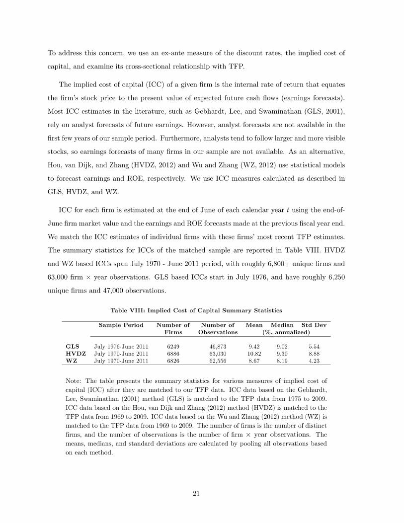
The summary statistics for ICCs of the matched sample are reported in Table VIII. HVDZ

and WZ based ICCs span July 1970 - June 2011 period, with roughly 6,800+ unique firms and

63,000 firm × year observations. GLS based ICCs start in July 1976, and have roughly 6,250

unique firms and 47,000 observations.

Table VIII: Implied Cost of Capital Summary Statistics

Sample Period Number of Number of Mean Median Std DevFirms Observations (%, annualized)

GLS July 1976-June 2011 6249 46,873 9.42 9.02 5.54HVDZ July 1970-June 2011 6886 63,030 10.82 9.30 8.88WZ July 1970-June 2011 6826 62,556 8.67 8.19 4.23

Note: The table presents the summary statistics for various measures of implied cost ofcapital (ICC) after they are matched to our TFP data. ICC data based on the Gebhardt,Lee, Swaminathan (2001) method (GLS) is matched to the TFP data from 1975 to 2009.ICC data based on the Hou, van Dijk and Zhang (2012) method (HVDZ) is matched to theTFP data from 1969 to 2009. ICC data based on the Wu and Zhang (2012) method (WZ) ismatched to the TFP data from 1969 to 2009. The number of firms is the number of distinctfirms, and the number of observations is the number of firm × year observations. Themeans, medians, and standard deviations are calculated by pooling all observations basedon each method.

21

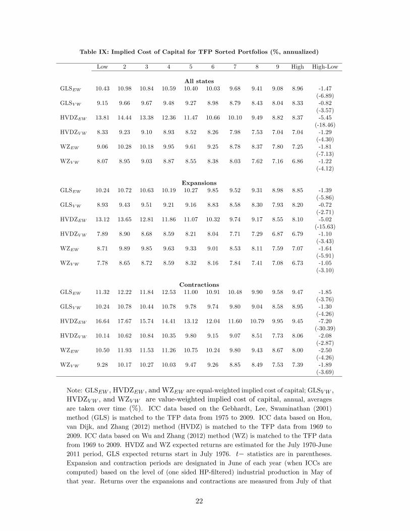
Table IX: Implied Cost of Capital for TFP Sorted Portfolios (%, annualized)

Low 2 3 4 5 6 7 8 9 High High-Low

All statesGLSEW 10.43 10.98 10.84 10.59 10.40 10.03 9.68 9.41 9.08 8.96 -1.47

(-6.89)GLSVW 9.15 9.66 9.67 9.48 9.27 8.98 8.79 8.43 8.04 8.33 -0.82

(-3.57)HVDZEW 13.81 14.44 13.38 12.36 11.47 10.66 10.10 9.49 8.82 8.37 -5.45

(-18.46)HVDZVW 8.33 9.23 9.10 8.93 8.52 8.26 7.98 7.53 7.04 7.04 -1.29

(-4.30)WZEW 9.06 10.28 10.18 9.95 9.61 9.25 8.78 8.37 7.80 7.25 -1.81

(-7.13)WZVW 8.07 8.95 9.03 8.87 8.55 8.38 8.03 7.62 7.16 6.86 -1.22

(-4.12)

ExpansionsGLSEW 10.24 10.72 10.63 10.19 10.27 9.85 9.52 9.31 8.98 8.85 -1.39

(-5.86)GLSVW 8.93 9.43 9.51 9.21 9.16 8.83 8.58 8.30 7.93 8.20 -0.72

(-2.71)HVDZEW 13.12 13.65 12.81 11.86 11.07 10.32 9.74 9.17 8.55 8.10 -5.02

(-15.63)HVDZVW 7.89 8.90 8.68 8.59 8.21 8.04 7.71 7.29 6.87 6.79 -1.10

(-3.43)WZEW 8.71 9.89 9.85 9.63 9.33 9.01 8.53 8.11 7.59 7.07 -1.64

(-5.91)WZVW 7.78 8.65 8.72 8.59 8.32 8.16 7.84 7.41 7.08 6.73 -1.05

(-3.10)

ContractionsGLSEW 11.32 12.22 11.84 12.53 11.00 10.91 10.48 9.90 9.58 9.47 -1.85

(-3.76)GLSVW 10.24 10.78 10.44 10.78 9.78 9.74 9.80 9.04 8.58 8.95 -1.30

(-4.26)HVDZEW 16.64 17.67 15.74 14.41 13.12 12.04 11.60 10.79 9.95 9.45 -7.20

(-30.39)HVDZVW 10.14 10.62 10.84 10.35 9.80 9.15 9.07 8.51 7.73 8.06 -2.08

(-2.87)WZEW 10.50 11.93 11.53 11.26 10.75 10.24 9.80 9.43 8.67 8.00 -2.50

(-4.26)WZVW 9.28 10.17 10.27 10.03 9.47 9.26 8.85 8.49 7.53 7.39 -1.89

(-3.69)

Note: GLSEW , HVDZEW , andWZEW are equal-weighted implied cost of capital; GLSVW ,HVDZVW , and WZVW are value-weighted implied cost of capital, annual, averagesare taken over time (%). ICC data based on the Gebhardt, Lee, Swaminathan (2001)method (GLS) is matched to the TFP data from 1975 to 2009. ICC data based on Hou,van Dijk, and Zhang (2012) method (HVDZ) is matched to the TFP data from 1969 to2009. ICC data based on Wu and Zhang (2012) method (WZ) is matched to the TFP datafrom 1969 to 2009. HVDZ and WZ expected returns are estimated for the July 1970-June2011 period, GLS expected returns start in July 1976. t− statistics are in parentheses.Expansion and contraction periods are designated in June of each year (when ICCs arecomputed) based on the level of (one sided HP-filtered) industrial production in May ofthat year. Returns over the expansions and contractions are measured from July of that

22

year to June of the following year.

Table IX presents the average implied cost of capital estimates for portfolios sorted on

productivity. The relationship between TFP and the cost of capital measured from all three ICC

measures is negative and quite monotonic. The firms with low productivity have higher discount

rates (ICC) than firms with high productivity using all ICC measures and both for equal and

value weighted portfolios. The spreads between the high and low TFP firms’expected returns

are all negative and highly statistically significant, implying that firms with low productivity

have higher ex-ante discount rates, and so are riskier than high productivity firms.

In addition to the unconditional discount rates, Table IX also presents the ICCs conditional

on whether the economy is expanding or contracting around the portfolio formation time.

Similar to the results based on average realized returns in Table IV, both the levels of implied

cost of capital and the spread between the low and high TFP portfolios are countercyclical. The

spreads between the discount rates of low and high TFP portfolios increase roughly 50-100%

for all ICC measures and for both equal and value-weighted portfolios as the economy moves

from expansions to contractions. However, most of the increases in expected returns happen in

the low TFP portfolio returns. Even though all firms are riskier in recessions, firms with low

productivity are hit particularly hard and thus bear more risk than firms with high TFPs.

1.4.4 Inspecting the Mechanism with Operating Performance

We have shown that firm level TFPs are systematically related to many firm characteristics and

firms with low TFP have higher future realized returns and implied cost of capital. Furthermore,

we document that the return spreads between the low and high TFP firms increase during

recessions, and this increase is mostly due to a surge in expected returns of low TFP firms. Our

interpretation of this return evidence is that low TFP firms are riskier than high TFP firms,

and they are particularly risky in recessions. In this section, we provide additional evidence on

the higher risk of low TFP firms that is not based on realized or ex-ante returns. We investigate

whether there are systematic differences in the sensitivity of low and high TFP firms’operating

performance to aggregate shocks in the economy. The existence of such differences would shed

some light on the mechanism behind the risk and return differentials between low and high

TFP firms.

23

We conjecture that operating performance of low TFP firms would be more sensitive to

aggregate shocks than the high TFP firms, especially during bad economic times. We measure

the operating performance of firms with their profitability. In order to test this hypothesis, we

examine pooled time series/cross sectional regressions of the form:

∆Profitit = b0 + b1∆Profitagg,t + b2∆Profitagg,t × IPt−1 + εit (4)

where ∆Profiti,t is the change in the profits (net income) of firm i between year t − 1 and

t, scaled by firm’s assets in year t − 1.24 We proxy aggregate shocks with the cross sectional

average of ∆Profiti,t over all firms in our sample.25 Our business cycle variable is the one

sided HP-filtered industrial production, defined earlier in Section 1.4.1, standardized to have a

standard deviation of 1. Industrial production is measured in May of year t − 1 (released in

June). We separate firms into 10 TFP groups based on their TFPs in year t− 1, similar to the

decile portfolios used earlier. We run panel regressions for in each TFP group.

Table X reports the results of the profitability regressions. Examination of Panel A reveals

that, unconditionally, low TFP firms have higher sensitivity to aggregate shocks in the economy.

The regression coeffi cient is 1.5 for the firms in the lowest TFP group, goes down to around

0.8 for higher TFP groups, and increases to 1.1 for the firms in the highest TFP group. More

importantly, Panel B shows that low TFP firms’sensitivity to aggregate shocks increases in

bad economic times (when industrial production is low). One standard deviation decrease in

industrial production increases the sensitivity of lowest TFP firms by approximately 0.5. The

pattern reverses for high TFP firms: Their profits’sensitivity to aggregate shocks increases in

good times by approximately 0.3. These results are consistent with our earlier findings based on

returns/discount rates and imply a higher risk for low TFP firms, especially when the economy

is doing poorly.

24This regression is obtained from writing our empirical model in levels with year and firm fixed effects andthen taking the first differences, which leads to the elimination of year and firm fixed effects.25Replacing ∆Profitagg,t with change in aggregate labor productivity reported by the BLS yields similar results.

Note that we cannot calculate aggregate productivity by averaging our firm level TFPs as our TFP estimatesare free of industry and year effects. Using ∆Profit on each side of the regression, at the firm level on the LHSand aggregate on the RHS, brings a beta-like interpretation to the regression coeffi cients.

24

Table X: Profitability Regressions for TFP Sorted PanelsDependent Variable: ∆Profiti,t

Low TFP 2 3 4 5 6 7 8 9 High TFP

Panel Aintercept 0.04 0.00 0.00 -0.01 -0.01 -0.01 0.00 -0.01 -0.01 -0.01

(7.47) (0.44) (0.32) (-6.41) (-6.01) (-3.97) (-2.60) (-4.27) (-2.17) (-1.92)

∆Profitagg,t 1.53 1.34 0.81 1.01 1.01 0.93 0.66 0.82 0.86 1.09(3.52) (8.04) (7.15) (10.89) (9.75) (6.02) (8.26) (7.35) (5.00) (4.00)

Panel Bintercept 0.05 0.00 0.00 -0.01 -0.01 -0.01 0.00 -0.01 -0.01 -0.01

(7.38) (1.15) (0.38) (-6.81) (-5.67) (-5.17) (-2.96) (-3.83) (-2.13) (-2.03)

∆Profitagg,t 1.11 1.05 0.77 0.95 0.95 1.06 0.74 0.99 0.99 1.35(2.70) (9.27) (6.10) (12.58) (10.13) (9.98) (12.14) (8.66) (4.96) (4.98)

∆Profitagg,t -0.56 -0.38 -0.04 -0.08 -0.07 0.17 0.10 0.23 0.17 0.33×IPt−1 (-2.95) (-4.62) (-0.88) (-1.26) (-1.05) (1.83) (2.09) (3.78) (2.82) (2.93)

Note: The table presents the results of panel regressions of change in firm level profitabil-ity on change in aggregate profitability and change in aggregate profitability conditionalon past industrial production. Change in profitability is measured as the level differencebetween current and past profits, scaled by lagged assets. Change in aggregate profitabilityis measured as the cross sectional average of firm level changes. Industrial production is thelevel of (one sided HP-filtered) industrial production in May of the past year, standardizedto have a standard deviation of 1. Firms are sorted into 10 equal-sized TFP groups based onpast year’s TFPs. The sample period is 1964-2009, total number of observations is 78,382.Standard errors are clustered by date and t− statistics are in parentheses.

2 Model

In this section we investigate whether a model where firms are subject to both aggregate and

idiosyncratic productivity shocks is capable of accounting for the cross sectional relationship

between TFP, firm level characteristics, and stock returns documented in Tables III, IV, and

V. We calibrate the model using the firm level TFP estimates summarized in Section 1.2

and examine the resulting firm level characteristics and firm returns generated by the model

economy.

25

2.1 Firms

There are many firms that produce a homogeneous good using capital and labor. These firms

are subject to different productivity shocks.

The production function for firm i is given by:

Yit = F (At, Zit,Kit, Lit)

= AtZitKαkit L

αlit .

Kit denotes the beginning of period t capital stock of firm i. Lit denotes the labor used in

production by firm i during period t. Labor and capital shares are given by αl and αk where

αl + αk ∈ (0, 1). Aggregate productivity is denoted by at = log (At) . at has a stationary and

monotone Markov transition function, given by pa (at+1|at), as follows:

at+1 = ρaat + εat+1 (5)

where εat+1 ∼ i.i.d. N(0, σ2

a

). The firm productivity, zit = log(Zit), has a stationary and

monotone Markov transition function, denoted by pzi(zi,t+1|zit), as follows:

zi,t+1 = ρzzit + εzi,t+1 (6)

where εzi,t+1 ∼ i.i.d. N(0, σ2

z

). εzi,t+1 and ε

zj,t+1 are uncorrelated for any pair of firms (i, j) with

i 6= j.

The capital accumulation rule is:

Ki,t+1 = (1− δ)Kit + Iit

where Iit denotes investment and δ denotes the depreciation rate of installed capital.

Investment is subject to quadratic adjustment costs given by git:

g (Iit,Kit) =1

2η

(IitKit− δ)2

Kit (7)

with η > 0. In this specification, investors incur no adjustment cost when net investment is

26

zero, i.e., when the firm replaces its depleted capital stock and maintains its capital level.

Firms are equity financed and face a perfectly elastic supply of labor at a given stochastic

equilibrium real wage rate Wt as in Bazdresch, Belo, and Lin (2010) and Jones and Tüzel

(Forthcoming). The equilibrium wage rate, given by:

Wt = exp(ωat) (8)

is assumed to be increasing with aggregate productivity, with 0 < ω < 1 determining the

sensitivity of the relation.26 Hiring decisions are made after firms observe the productivity

shocks and labor is adjusted freely; hence, for each firm, marginal product of labor equals the

wage rate:

FLit = FL(At, Zit,Kit, Lit)

= Wt.

Dividends to shareholders are equal to:

Dit = Yit − [Iit + git]−WtLit. (9)

At each date t, firms choose {Ii,t, Li,t} to maximize the net present value of their expected

dividend stream, which is the firm value:

Vit = max{Ii,t+k,Li,t+k}

Et

[ ∞∑k=0

Mt,t+kDi,t+k

], (10)

subject to (Eq.5-8), where Mt,t+k is the stochastic discount factor between time t and t+k. Vit

is the cum-dividend value of the firm.

The first order conditions for the firm’s optimization problem leads to the pricing equation:

1 =

∫ ∫Mt,t+1R

Ii,t+1pzi(zi,t+1|zit)pa(at+1|at)dzida (11)

26With competitive labor markets, wage equals the value of the marginal product of labor. In general equilib-rium with a representative firm, the marginal product of labor is mpl = exp(at)αlL

αl−1Kαk . Hence, wages are afunction of aggregate productivity, total labor force, and the capital stock used in production. Here we abstractfrom aggregate labor and capital and model wages as a function of aggregate productivity.

27

where the returns to investment are given by:

RIi,t+1 =

FKi,t+1 + (1− δ)qi,t+1 + 12η

((Ii,t+1Ki,t+1

)2− δ2

)qit

(12)

and where

FKit = FK(At, Zit,Kit, Lit).

Tobin’s q, the consumption good value of a newly installed unit of capital, is:

qit = 1 + η

(IitKit− δ). (13)

The pricing equation (Eq.11) establishes a link between the marginal cost and benefit of

investing. The term in the denominator of the right hand side of the equation, qit, measures

the marginal cost of investing. The terms in the numerator represent the discounted marginal

benefit of investing. The firm optimally chooses Iit such that the marginal cost of investing

equals the discounted marginal benefit.

The returns to the firm are defined as:27

RSi,t+1 =Vi,t+1

Vit −Dit. (14)

2.2 The Stochastic Discount Factor

Since the purpose of our model is to examine the cross sectional variation across firms, we use

a framework where time series properties of returns are matched by using an exogenous pricing

kernel. Following Berk, Green, and Naik (1999), Zhang (2005), and Gomes and Schmid (2010),

we directly parameterize the pricing kernel without explicitly modeling the consumer’s problem.

As in Jones and Tüzel (Forthcoming), the pricing kernel is given by:

logMt+1 = log β − γtεat+1 −1

2γ2tσ

2a (15)

log γt = γ0 + γ1at

27We do not assume constant returns to scale in the production function; i.e.,αl + αk ∈ (0, 1). In the presenceof constant returns to scale, firm return would be equivalent to the returns to fixed investment, RIt+1. Withslightly decreasing returns to scale, firm returns slightly diverge from the investment returns.

28

where β, γ0 > 0, and γ1 < 0 are constant parameters.

This pricing kernel shares a number of similarities with Zhang (2005). Mt+1, the stochastic

discount factor from time t to t+ 1, is driven by εat+1, the shock to the aggregate productivity

process in period t+ 1. The volatility of Mt+1 is time-varying, driven by the γt process. This

volatility takes higher values following business cycle contractions and lower values following

expansions, implying a countercyclical price of risk as the result.28 In the absence of counter-

cyclical price of risk, the risk premia generated in the economy does not change with economic

conditions. Empirically, existence of time varying risk premia is well documented (Fama and

Schwert (1977); Fama and Bliss (1987); Fama and French (1989); Campbell and Shiller (1991);

Cochrane and Piazzesi (2005); Jones and Tüzel (2013); among many others). Our empirical

results in Table IV and Table IX, that average (future) realized returns and implied cost of

capital are much higher in contractions, compared to expansions, provide additional motivation

for modeling countercyclical price of risk.

2.3 Calibration

Solving our model generates firms’ investment and hiring decisions as functions of the state

variables, which are the aggregate and firm level productivity and the capital of the firm. Since

the stochastic discount factor and the wages are specified exogenously, the solution does not

require aggregation. Hence, the distribution of the capital stock, a high dimensional object is

not a part of the state space. This feature of the model simplifies the solution of the model

significantly.

To be consistent with our annual empirical results, we calibrate the model at annual fre-

quency. Table XI presents the parameters used in the calibration.29 We derive the parameters

of the firm level productivity process from the production function estimations in Section 1.2.

The persistence of the firm productivity process, ρz, is 0.7. The conditional volatility of firm

productivity, σz, is computed from ρz and the cross sectional standard deviation of firm pro-

28A countercyclical price of risk is endogenously derived in Campbell and Cochrane (1999) from time varyingrisk aversion; in Barberis, Huang, and Santos (2001) from loss aversion; in Constantinides and Duffi e (1996)from time varying cross sectional distribution of labor income; in Guvenen (2009) from limited participation; inBansal and Yaron (2004) from time varying economic uncertainty; and in Piazzesi, Schneider, and Tüzel (2007)from time varying consumption composition risk.29Calibration of the model economy based on alternative TFP estimations (summarized in the Appendix)

yields very similar asset pricing results.

29

ductivity as 0.268(

= 0.38×√

1− 0.72).30 The parameters of the production function, αk and

αl, are roughly equal to our estimates presented in Table I and Figure 1. Even though our

production function estimates imply almost constant returns to scale production technology,

we model technology as slightly decreasing returns to scale, with αk + αl = 0.95. It is well

known that firm size is indeterminate with constant returns to scale technology. Decreasing

returns to scale technology makes studying the relationship between firm size and productivity

possible.

Table XI: Model Parameter Values

Parameter Description Value

αk Capital share 0.22αl Labor share 0.73ω Wage sensitivity to aggregate productivity 0.20β Discount factor 0.988γ0 Constant price of risk parameter 3.27γ1 Time varying price of risk parameter -13.32δ Capital depreciation rate 0.08η Adjustment cost parameter 4.45ρa Persistence of aggregate productivity 0.922σa Conditional volatility of aggregate productivity 0.014ρz Persistence of firm productivity 0.7σz Conditional volatility of firm productivity 0.268

We take the parameters of the aggregate productivity from King and Rebelo (1999) and

annualize them. Their point estimates for ρa and σa are 0.979 and 0.0072, respectively, using

quarterly data, implying annual parameters of 0.922 and 0.014. The depreciation rate for fixed

capital is set to 8% annually, which is roughly the midpoint of values used in other studies.

Cooley and Prescott (1995) use 1.6%; Boldrin, Christiano, and Fisher (2001) use 2.1%; and

Kydland and Prescott (1982) use a 2.5% quarterly depreciation rate. We follow Bazdresch,

Belo, and Lin (2010) in choosing the wage function parameter ω to equal 0.2, which matches

the aggregate wage cyclicality estimated by Merz and Yashiv (2007).

We choose the pricing kernel parameters β, γ0, and γ1 to match the average riskless rate

and the first two moments of aggregate value-weighted excess stock returns measured from the

data used in our empirical exercise. The discount factor β is 0.988, which implies an annual

risk free rate of 1.2%. γ0 and γ1 are 3.27 and −13.32, respectively, and generate annual excess

mean returns and standard deviation of 6.16% and 17%, respectively. Finally, the adjustment

30The dispersion of firm productivity rises over time, from 0.23 in 1963 to 0.53 in 2009. In this calibration, wetake the cross sectional standard deviation to be 0.375, which is the average dispersion over this time period.

30

cost parameter, η, is set to 4.45 to replicate the value-weighted average (annual) volatility of

investment to capital ratio of 15.7% in our data.

In order to compute the model statistics, we perform 500 simulations of the model economy

with 1,000 firms over 50 periods (years), which is roughly comparable to the length and average

breadth of our empirical sample.

2.4 Model Results

The key mechanism relating firm level productivity to expected returns involves the interaction

of convex adjustment costs and the countercyclical Sharpe ratios assumed in our pricing kernel.

Firm risk derives from its inability to freely adjust its capital following shocks to aggregate

and firm level productivity. In this economy, aggregate productivity shocks drive the business

cycles. In bad times (low aggregate productivity level), net present value of investments go

down due to lower expected cash flows and higher discount rates. Hence, all firms would like to

invest less and hire less. Even though firms can freely adjust their labor, they incur adjustment

costs when they change their capital stock.31 In states of low aggregate productivity, a bad

aggregate shock has a larger negative effect on the low TFP firms. These firms would have a

lower investment rate (i.e., reduce their capital stock relatively more) than the high TFP firms.

Due to the convexity in adjustment costs, low TFP firms, who are at a steeper part of the

adjustment costs, sustain a higher cost while reducing their capital stock in a recession than

high TFP firms. A positive aggregate shock, on the other hand, results in a bigger decrease in

adjustment costs for these firms compared to more productive firms, hence benefiting the low

TFP firms more than the others. Therefore, the returns of the low TFP firms covary more with

changes in the economic conditions during recessions. The opposite happens in expansions.32

The countercyclical Sharpe ratio breaks the symmetry between recessions and expansions.33

31Note that adjustment costs are defined over net investment, rather than gross investment. Hence, adjustmentcosts are high when investment is higher, as well as lower than depreciated capital.32Unlike Zhang (2005) and many other papers in this literature, our model does not have operating leverage

(fixed cost of production). Operating leverage helps those models to magnify the differences between low and highproductivity firms since they disproportionately affect the low productivity firms. Like Tüzel (2010); Bazdresch,Belo, and Lin (2009); and Tüzel and Jones (Forthcoming), our model features labor as a factor of production.Marginal product of labor across firms is equalized as labor is free to move between them. This leads to vastlydifferent optimal hiring and investment decisions between firms and generates significant heterogeneity withoutincorporating operating leverage.33For simplicity, we assume symmetric adjustment costs, but asymmetric adjustment costs as in Zhang (2005)

or Tüzel (2010) would also break this symmetry and strengthen our results.

31

We assume that the volatility of the pricing kernel is a decreasing function of aggregate produc-

tivity; hence, Sharpe ratios (and discount rates) are higher in bad times. Risk is defined as the

covariation of the returns with the pricing kernel. Higher volatility of the pricing kernel implies

higher covariation with the kernel, hence higher risk in bad times. Lower rates of investment

of low productivity firms tend to occur during recessions when Sharpe ratios are high, mak-

ing them especially risky. Therefore, low productivity firms, during economic downturns, have

the highest expected returns. These firms are the primary drivers of negative cross sectional

relations between expected returns and firm productivity. Higher rates of investment of high

productivity firms, on the other hand, tend to occur during expansionary periods when Sharpe

ratios are low, and therefore result in lower expected returns for these firms.

In order to demonstrate the effect of aggregate shocks on low and high TFP firms over the

business cycle, Figure 2 plots the sensitivity of low and high TFP firms’returns to aggregate

TFP shocks conditional on the state of the economy. Good (bad) times are defined as times

when the last period’s aggregate TFP is more than one standard deviation above (below) its

mean. Low (high) TFP firms are firms in the lowest (highest) TFP decile based on last year’s

ranking. The top panel plots the aggregate shock - realized return (averaged over all low or

high TFP firms every period) relationship in good times, the bottom panel plots the same in

bad times. There is a positive relationship between aggregate shocks and realized returns for all

firms and economic environments. However, the relationship is quite flat for all firms in good

times, whereas the sensitivity of all firms, but especially the low TFP firms, is much higher in

bad times. These are the times when low TFP firms are the riskiest. Bad aggregate shocks

lead to very negative returns, whereas good shocks drive the high returns of low TFP firms in

bad times.

Table XII presents the results on the cross section of firms. Similar to our empirical analysis

in Sections 1.3 and 1.4.1, we form decile portfolios by sorting firms on the basis of past TFP

level. The table shows average firm characteristics and expected returns of these portfolios as

well as the spreads between the low and high portfolios. We also present confidence intervals

around the model-implied values of the spreads in returns. The results indicate that the model

is able to match the data presented in Tables III and IV reasonably well. The parameters of the

firm level TFP process are taken from the empirical estimates, so it is not surprising that the

average TFP of the simulated portfolios are matched almost exactly to the data. However, the

32

­0.04 ­0.03 ­0.02 ­0.01 0 0.01 0.02 0.03 0.04­1

0

1

2

3Good times

Aggregate TFP shock

% R

ealiz

ed re

turn

High TfpLow Tfp

­0.04 ­0.03 ­0.02 ­0.01 0 0.01 0.02 0.03 0.04­1

0

1

2

3Bad times

Aggregate TFP shock

% R

ealiz

ed re

turn

High TfpLow Tfp

Figure 2: Sensitivity of firm returns to aggregate shocks. Top figure plots the realized returnsas a function of aggregate productivity for low TFP and high TFP firms in good times. Bottomfigure plots the realized returns in bad times.

model is not calibrated to match the cross section of the remaining characteristics, namely the

investment to capital ratio, the hiring rate, firm size, book to market ratio, and the expected

returns. We find that the investment to capital ratio and hiring rate both increase monotonically

with TFP. Productive firms rationally invest and hire more than the unproductive firms since

both capital and labor will be more effi cient (their net present value would be higher) for

those firms. The dispersion in investment to capital ratios generated by the model economy is

reasonably close to what we observe in the data (0.3 versus 0.22), the dispersion in hiring rates

of low versus high productivity firms is an order of magnitude bigger in the model.34

TFP is also monotonically and positively related to size and negatively related to B/M. In

34This problem could be alleviated by introducing adjustment costs in hiring/firing, which is currently assumedto be costless. Adjustment costs in hiring would reduce the volatility in hiring rate, and hence reduce thedispersion in the hiring rate of the most productive and least productive firms.

33

the model, firm size is the ex-dividend value of the firm, Vit−Dit, which is approximately equal

to qtKt+1 (the amount of capital, Kt+1, × Tobin’s q, qit).35 Tobin’s q is linear in investment

to capital ratio (Eq. 13), which is monotonically increasing in TFP. Likewise, the amount of

capital, Kt+1, is increasing in TFP due to the positive relationship between investment and TFP

and the persistence in productivity. Therefore, we expect to see a positive relationship between

TFP and firm size. B/M, the ratio of book value to the market value of the firm, is measured

as the amount of capital, Kit+1, divided by the ex-dividend value of the firm, Vit−Dit. Hence,

B/M is approximately equal to the inverse of the Tobin’s q (qit) in the model.36 This leads to

a negative relationship between B/M and TFP. The model is quite successful in matching the

magnitude of the dispersion in B/M (-0.63 versus -0.87). Also, the model is able to capture

about half of the size dispersion found in the data (1.60 versus 3.53). These results indicate

that TFP shock alone can account for a significant fraction of the cross sectional dispersion in

firm characteristics found in the data.

Table XII also reports that the expected returns of TFP sorted portfolios decline monoton-

ically with TFP. The spread in expected returns, −7.99%, is close to the empirical spread of

−7.65% reported in Table IV. These returns are calculated by weighting the firms in the port-

folios equally, but, value-weighting the portfolios leads to quantitatively very similar results.

Furthermore, consistent with our empirical findings, both the average expected returns and

the spread between the low and high TFP portfolio returns are much higher in contractions,

compared to expansions. For this exercise, each year, we define periods where aggregate pro-

ductivity is more than one standard deviation lower than the mean (based on short sample

statistics) as contractions, and the remaining periods as expansions. This definition leads to

designating roughly 15% of the sample period as contractions, which is in line with the frequency

of contractionary periods in the data (96 out of 564 months in our sample period). The excess

returns are measured in the following year. The model generates −6.74% and −11.08% spread

in returns of TFP sorted portfolios in expansions and contractions, respectively. The empirical

spreads in expansions and contractions, −5.46% and −18.28%, respectively, both fall within

the wide confidence intervals around the model generated spread point estimates. However,

as in Lin and Zhang (2012), the model does not generate a significant spread in unconditional

35 In the presence of constant returns to scale, Vit −Dit = qtKt+1. With decreasing returns to scale, Vit −Ditslightly exceeds qtKt+1.36M/B would be exactly equal to Tobin’s q when the production technology is constant returns to scale.

34

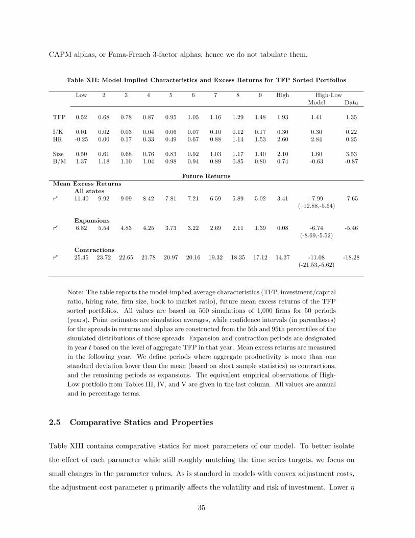
CAPM alphas, or Fama-French 3-factor alphas, hence we do not tabulate them.

Table XII: Model Implied Characteristics and Excess Returns for TFP Sorted Portfolios

Low 2 3 4 5 6 7 8 9 High High-LowModel Data

TFP 0.52 0.68 0.78 0.87 0.95 1.05 1.16 1.29 1.48 1.93 1.41 1.35

I/K 0.01 0.02 0.03 0.04 0.06 0.07 0.10 0.12 0.17 0.30 0.30 0.22HR -0.25 0.00 0.17 0.33 0.49 0.67 0.88 1.14 1.53 2.60 2.84 0.25

Size 0.50 0.61 0.68 0.76 0.83 0.92 1.03 1.17 1.40 2.10 1.60 3.53B/M 1.37 1.18 1.10 1.04 0.98 0.94 0.89 0.85 0.80 0.74 -0.63 -0.87

Future ReturnsMean Excess Returns

All statesre 11.40 9.92 9.09 8.42 7.81 7.21 6.59 5.89 5.02 3.41 -7.99 -7.65

(—12.88,-5.64)

Expansionsre 6.82 5.54 4.83 4.25 3.73 3.22 2.69 2.11 1.39 0.08 -6.74 -5.46

(-8.69,-5.52)

Contractionsre 25.45 23.72 22.65 21.78 20.97 20.16 19.32 18.35 17.12 14.37 -11.08 -18.28

(-21.53,-5.62)

Note: The table reports the model-implied average characteristics (TFP, investment/capitalratio, hiring rate, firm size, book to market ratio), future mean excess returns of the TFPsorted portfolios. All values are based on 500 simulations of 1,000 firms for 50 periods(years). Point estimates are simulation averages, while confidence intervals (in parentheses)for the spreads in returns and alphas are constructed from the 5th and 95th percentiles of thesimulated distributions of those spreads. Expansion and contraction periods are designatedin year t based on the level of aggregate TFP in that year. Mean excess returns are measuredin the following year. We define periods where aggregate productivity is more than onestandard deviation lower than the mean (based on short sample statistics) as contractions,and the remaining periods as expansions. The equivalent empirical observations of High-Low portfolio from Tables III, IV, and V are given in the last column. All values are annualand in percentage terms.

2.5 Comparative Statics and Properties

Table XIII contains comparative statics for most parameters of our model. To better isolate

the effect of each parameter while still roughly matching the time series targets, we focus on

small changes in the parameter values. As is standard in models with convex adjustment costs,

the adjustment cost parameter η primarily affects the volatility and risk of investment. Lower η

35

leads to higher investment volatility, lower risk, and lower expected returns in the economy. In

the cross section, however, differences in investment behavior fueled by lower η leads to bigger

dispersion between the low and high TFP firms.

Changing the pricing kernel parameters γ0 and γ1 yields predictable results. While the two

parameters play different roles, an increase in the absolute value of either parameter will raise

the equity premium, and return spreads rise in an approximately proportional manner. As a

result of greater variation in expected returns, investment becomes slightly more volatile as

well.

Finally, lowering the sensitivity of wages to aggregate productivity (lower ω) increases the

risk and risk premia. This is due to the fact that wages do not fall as far in recessions or rise

as much in expansions, causing firms to make bigger adjustments to the quantity of labor and

leading to larger fluctuations in output. This effect also causes higher volatility in investment.

Table XIII: Comparative Statics

Decile portfolio spreads inCase E(re) Std

(IK

)IK

HR Size B/M E(re)

Benchmark 6.16 15.66 0.30 2.84 1.60 -0.63 -7.99

low η η = 4 5.90 16.65 0.31 2.85 1.63 -0.64 -8.08high η η = 5 6.43 14.61 0.28 2.83 1.56 -0.63 -7.91

low γ0 γ0 = 3.24 6.01 15.23 0.29 2.84 1.57 -0.63 -7.23high γ0 γ0 = 3.30 6.17 16.11 0.30 2.85 1.69 -0.64 -8.79

low γ1 γ1 = −13.2 6.07 15.60 0.29 2.84 1.59 -0.63 -7.86low γ1 γ1 = −13.4 6.22 15.71 0.30 2.84 1.60 -0.64 -8.07

low ω ω = 0.1 6.19 15.80 0.30 2.84 1.66 -0.63 -7.97high ω ω = 0.3 5.87 15.53 0.30 2.84 1.65 -0.63 -8.01

Note: The table presents the comparative statics for our benchmark calibration. The toprow shows moments from the calibrated model, whose parameters are reported in Table XI.The rows beneath show the moments that result from changing one parameter to the valuegiven. Moments include E(re), the market risk premium, Std

(IK

), the average firm-level

volatility of investment, and the average spreads in investment to capital ratio, hiring rate,size, B/M ratio, and mean excess returns on TFP-sorted portfolios. All results are obtainedfrom 500 simulations of 1,000 firms for 50 periods (years).

Model parameters, calibrated as described in Section 2.3, often have implications for other

statistics as well. The parameter γ1 governs the degree of countercyclicality of the market price

of risk and also has implications on the degree of predictability in stock returns. In order to

36

test whether our benchmark value of -13.32 implies a realistic amount of predictability, we run

return predictability regressions where annual excess stock returns are predicted by our state

variable, aggregate TFP. We find that aggregate TFP predicts stock returns with 9.4% R2 at

annual horizon37, which is in line with the stock predictability regression R2’s reported in the

literature (Jones and Tüzel (2013)).

The adjustment cost parameter η also has additional implications for the economy. Lower

adjustment costs would imply higher elasticity of investment rate to Tobin’s q. Our benchmark

value of 4.45 generates an investment - q elasticity of 2.8 around the steady state. Due to

the poor empirical fit of the neoclassical investment equation, it is hard to find good empirical

estimates for this elasticity. The results in Cummins, Hassett, and Oliner (2006) imply an

elasticity around 1.2. Hence, our elasticity of 2.8 indicates a relatively low adjustment cost.

With this calibration, the fraction of output that is lost due to capital adjustment costs is

around 5%.

The functional form we assume for the equilibrium wage rate has implications for the cycli-

cality of aggregate employment in the economy. To compare the cyclical behavior generated

by our model to the data, we compute the correlation of total employment growth with output

growth, and the volatility of employment growth relative to output. We find that the moments

generated by the model measure up to the data well. In the postwar U.S. data, this correlation

is 0.9, and the relative volatility of employment growth is 1.1, while both of these numbers are

around 1 using the simulated data.

3 Conclusion

This paper provides new evidence about the link between TFP and stock returns, offering an

explanation to how firm characteristics can rationally predict returns. We estimate firm level

TFP and show that it is strongly related to several firm characteristics such as size, the book

to market ratio, investment, and hiring rate. TFP is negatively related to future stock returns,

as well as ex-ante discount rates. A production based asset pricing model calibrated to match

the estimated TFP distribution can replicate the empirical relationship between TFP, firm

37 In this regression and other model results, we compute statistics over short samples (50 periods) and reportthe average value from 500 simulations.

37

characteristics, and stock returns reasonably well. Firms that receive repeated bad shocks (low

TFP firms) end up being small firms and are characterized by low investment and hiring rates,

and high B/M ratio. High TFP firms are large firms with high investment and hiring rates, and

low B/M ratio. Low TFP firms end up being riskier than high TFP firms. Thus, differences in

TFP generates the observed relationships between characteristics and stock returns.

References

[1] Ball, R. 1978. Anomalies in Relationships Between Securities’Yields and Yield Surrogates.Journal of Financial Economics 6:103—26.

[2] Bansal, R. W. and A. Yaron. 2004. Risks For the Long Run: A Potential Resolution ofAsset Pricing Puzzles. Journal of Finance 59:1481-509.

[3] Banz, R. W. 1981. The Relationship Between Return and Market Value of Common Stocks.Journal of Financial Economics 9:3—18.

[4] Barberis, N., M. Huang and T. Santos. 2001. Prospect Theory and Asset Price. QuarterlyJournal of Economics 116:1-53.

[5] Bartelsman, E. J. and P. J. Dhrymes. 1998. Productivity Dynamics: U.S. ManufacturingPlants 1972-1986. Journal of Productivity Analysis 9:5-34.

[6] Basu, S. 1983. The Relationship Between Earnings Yield, Market Value, and Return forNYSE Common Stocks: Further evidence. Journal of Financial Economics 12:129—56.

[7] Bazdresch, S., F. Belo and X. Lin. 2010. Labor Hiring, Investment and Stock ReturnPredictability in the Cross Section. Working paper.

[8] Belo, F. and X. Lin. 2012. The Inventory Growth Spread. Review of Financial Studies25:278-313.

[9] Berk, J. B., R. C. Green and V. Naik. 1999. Optimal Investment, Growth Options, andSecurity Returns. Journal of Finance 54:1553-607.

[10] Bhandari, L. 1988. Debt/Equity Ratio and Expected Common Stock Returns: EmpiricalEvidence, Journal of Finance 43:507-28.

[11] Boldrin, M., L. Christiano and J. Fisher. 2001. Habit Persistence, Asset Returns, and theBusiness Cycle. American Economic Review 91:149-66.

[12] Brynjolfsson, E. and L. Hitt. 2003. Computing Productivity: Firm-Level Evidence. Reviewof Economics and Statistics 85:793-808.

[13] Campbell, J.Y. and J. H. Cochrane. 1999. By force of habit: a consumption-based expla-nation of aggregate stock market behavior. Journal of Political Economy 107:205—51.

[14] Campbell, J., and R. Shiller. 1991. Yield Spreads and Interest Rate Movements: A Bird’sEye View. Review of Economic Studies 58:495-514.

38

[15] Chan, L. K.C., N. Jegadeesh, and J. Lakonishok. 1996. Momentum Strategies. Journal ofFinance 51:1681-713.

[16] Cochrane, J. H., and M. Piazzesi. 2005. Bond Risk Premia. American Economic Review95:138-60.

[17] Constantinides, G. and D. Duffi e. 1996. Asset Pricing with Heterogeneous Consumers.Journal of Political Economy 104:219—240.

[18] Cooley, T. F., and E. C. Prescott. 1995. Economic Growth and Business Cycles. In T. F.Cooley (ed.), Frontiers of Business Cycle Research, Princeton University Press.

[19] Cooper, I., H. Gulen and M. Schill. 2008. Asset Growth and the Cross-Section of StockReturns. Journal of Finance 63:1609-52.

[20] Cummins, J. G., K. A. Hassett and S. D. Oliner. 2006. Investment Behavior, ObservableExpectations, and Internal Funds. American Economic Review 96:796-810.

[21] De Bondt,W. F. M., and R. Thaler. 1985. Does the Stock Market Overreact?. Journal ofFinance 40:793—805.

[22] Dwyer, D. 1998. Technology Locks, Creative Destruction, and Non-Convergence in Pro-ductivity Levels. Review of Economic Dynamics 1:430-73.

[23] Eisfeldt, L. A. and D. Papanikolaou. Forthcoming. Organization Capital and the Cross-Section of Expected Returns. Journal of Finance.

[24] Fama, E., and R. Bliss. 1987. The Information in Long-Maturity Forward Rates. AmericanEconomic Review 77:680-92.

[25] Fama, E., and K. French. 1989. Business Conditions and Expected Returns on Stocks andBonds. Journal of Financial Economics 25:23-49.

[26] Fama, E. F. and K. French. 1992. The cross section of expected stock returns. The Journalof Finance 47:427-65.

[27] Fama, E. F. and K. R. French. 1993. Common Risk Factors in the Returns on Stocks andBonds. Journal of Financial Economics 33:3-56.

[28] Fama, E. F. and K. R. French. 2008. Dissecting anomalies. Journal of Finance 63:1653-78.

[29] Fama, E. F. and J. D. MacBeth. 1973. Risk, return, and equilibrium: Empirical tests.Journal of Political Economy 81:607-36.

[30] Fama, E., and W. Schwert. 1977. Asset Returns and Inflation. Journal of Financial Eco-nomics 5:115-46.

[31] Fernández-Villaverde, J. and J. F. Rubio-Ramírez. 2007. On the solution of the growthmodel with investment-specific technological change. Applied Economics Letters 14:533-49.

[32] Foster, L., J. Haltiwagner, and C. Syverson .2008 . Reallocation, Firm Turnover and Effi -ciency: Selection on Productivity or Profitability. American Economic Review 98:394-425.

39

[33] Gala, V. 2006. Irreversible Investment and the Cross-Section of Stock Returns in GeneralEquilibrium. Working paper.

[34] Garleanu, Nicolae, Panageas, Stavros and Jianfeng Yu (2012). Technological Growth andAsset Pricing. Journal of Finance 67:1265-1292.

[35] Gebhardt, W.R., C.M.C. Lee, and B. Swaminathan. 2001 . Toward an Implied Cost ofCapital. Journal of Accounting Research 39:135-76.

[36] Gomes, J. F. 2001. Financing Investment. American Economic Review 90:1263—85.

[37] Gomes, J. F., L. Kogan and L. Zhang. 2003. Equilibrium Cross-Section of Returns. Journalof Political Economy 111:693-732.

[38] Gomes, J. F. and L. Schmid. 2010. Levered Returns, Journal of Finance 65:467-94.

[39] Gourio, F. 2007. Labor Leverage, Firms’Heterogeneous Sensitivities to the Business Cycle,and the Cross-Section of Expected Returns. Working paper. Boston University

[40] Greenwood, J., Z. Hercowitz, and P. Krusell. 1997. Long-Run Implications of Investment-Specific Technological Change. American Economic Review 87:342-62.

[41] Greenwood, J., Z. Hercowitz, and P. Krusell. 2000. The Role of Investment-Specific Tech-nological Change in the Business Cycle. European Economic Review 44:91-115.

[42] Guvenen, F. 2009. A Parsimonious Macroeconomic Model for Asset Pricing. Econometrica77:1711-50.

[43] Hadlock, C. J. and J. R. Pierce. 2010. New Evidence on Measuring Financial Constraints:Moving Beyond the KZ Index. Review of Financial Studies 23:1909-40.

[44] Hall, B. H. 1990. The Manufacturing Sector Master File: 1959-1987. NBER Working paper3366.

[45] Hennessy, C. and T. Whited. 2005. Debt Dynamics. Journal of Finance 60:1129-65.

[46] Hou, K., A. M. van Dijk and Y. Zhang. 2012. The Implied Cost of Capital: A NewApproach. Journal of Accounting and Economics 53:504-26.

[47] Hulten, C. R. 1990. The Measurement of Capital. In Ernst R. Berndt and Jack E. Triplett(eds.), Fifty Years of Economic Measurement: The Jubilee of the Conference on Researchin Income and Wealth. NBER Studies in Income and Wealth 54:119-52. University ofChicago Press.

[48] Jegadeesh, N. and S. Titman. 1993. Returns to Buying Winners and Selling Losers: Im-plications for Stock Market Effi ciency. Journal of Finance 48:65-91.

[49] Jones, C. S., and S. Tüzel. Forthcoming. Inventory Investment and the Cost of Capital.Journal of Financial Economics.

[50] Jones, C. S., and S. Tüzel. 2013. New Orders and Asset Prices. Review of Financial Studies26:115-157.

40

[51] King, R. G. and S. T. Rebelo. 1999. Resuscitating Real Business Cycles. In J. B. Taylorand M. Woodford (ed.), Handbook of Macroeconomics, edition 1, chapter 14, 1:927-1007Elsevier.

[52] Kogan, L. and D. Papanikolaou. 2011. Growth Opportunities, Technology Shocks andAsset Prices. NBER Working paper No. 17795.

[53] Kovenock, D. and G. Phillips. 1997. Capital Structure and Product Market Behavior:An Examination of Plant Closing and Investment Decisions. Review of Financial Studies10:767-803.

[54] Kydland, F. and E. Prescott. 1982. Time to Build and Aggregate Fluctuations. Economet-rica 50:1345-70.

[55] Levinsohn, J. and A. Petrin. 2003. Estimating Production Functions Using Inputs to Con-trol for Unobservables. Review of Economic Studies 70:317—41.

[56] Li, E. X. N., D. Livdan and L. Zhang. 2009. Anomalies. Review of Financial Studies22:4301-34.

[57] Lieberman, M. and J. Kang. 2008. How to Measure Company Productivity using Value-added: A Focus on Pohang Steel (POSCO). Asia Pacific Journal of Management 25:209—24.

[58] Lin, Xiaoji and Lu Zhang. Forthcoming. The Investment Manifesto. Journal of MonetaryEconomics.

[59] Liu, L. X., T. M. Whited and L. Zhang. 2009. Investment-Based Expected Stock Returns.Journal of Political Economy 117:1105—39.

[60] Livdan, D., Sapriza, H. and Zhang, L. (2009). “Financially Constrained Stock Returns”,Journal of Finance 64, pages 1827-1862.

[61] Lyandres, E., L. Sun and L. Zhang. 2008. The New Issues Puzzle: Testing the Investment-Based Explanation. Review of Financial Studies 21:2825-55.

[62] McGuckin, R. H. and S. V. Nguyen. 1995. On Productivity and Plant Ownership Change:New Evidence from the LRD. RAND Journal of Economics 26:257-76.

[63] Merz, M. and E. Yashiv. 2007. Labor and the market value of the firm. American EconomicReview 97:1419-31.

[64] Novy-Marx, R. Forthcoming. The Other Side of Value: The Gross Profitability Premium.Journal of Financial Economics.

[65] Olley, S. and A. Pakes. 1996. The Dynamics Of Productivity In The TelecommunicationsEquipment Industry. Econometrica 64:1263-97.

[66] Pastor, L. and R. Stambaugh, 2003. Liquidity Risk and Expected Stock Returns. Journalof Political Economy 111:642—85.

[67] Philippon, T. 2009. The Bond Market’s Q. Quarterly Journal of Economics 124:1011-56.

41

[68] Piazzesi, M., M. Schneider and S. Tüzel. 2007. Housing, Consumption, and Asset Pricing.Journal of Financial Economics 83:531-69.

[69] Ravn, M. O., and H. Uhlig. 2002. On Adjusting the Hodrick-Prescott Filter for the Fre-quency of Observations. Review of Economics and Statistics 84:371-80.

[70] Schoar, A. 2002. Effects of Corporate Diversification on Productivity. Journal of Finance57:2379-403.

[71] Sloan, R. G. 1996. Do Stock Prices Fully Reflect Information in Accruals and Cash FlowsAbout Future Earnings?. The Accounting Review 71:289-315.

[72] Syverson, C. 2004. Product Substitutability and Productivity Dispersion. Review of Eco-nomics and Statistics 86:534-50.

[73] Thomas, J. K., and H. Zhang. 2002. Inventory Changes and Future Returns. Review ofAccounting Studies 7:163-87.

[74] Titman, S., K.C. J. Wei and F. Xie. 2003. Capital Investments and Stock Returns. Journalof Financial and Quantitative Analysis 39:677-700.

[75] Tüzel, S. 2010. Corporate Real Estate Holdings and the Cross Section of Stock Returns.Review of Financial Studies 23:2268-302.

[76] Wu, J. and L. Zhang. 2012. Do anomalies exist ex ante? Working paper, University ofGeorgia and Ohio State.

[77] Wu, J., L. Zhang and F. Zhang. 2010. The q-theory Approach to Understanding the AccrualAnomaly. Journal of Accounting Research 48:177-223.

[78] Zhang, L. 2005. Value premium. Journal of Finance 60:67-103.

42

4 Appendix

4.1 Measuring TFP

The main contributions to measuring firm level TFP are by Olley and Pakes (1996) and Levin-

sohn and Petrin (2003). The key difference between the two methods is that Olley and Pakes

(1996) use investment whereas Levinsohn and Petrin (2003) use materials used in production

as a proxy for TFP. Since data on investment is readily available and often non-zero at the

firm level but data on materials is not, we follow Olley and Pakes (1996) to estimate firm level

productivities.

In our benchmark case, we estimate the production function based on labor and physical

capital as inputs. The production technology is given by yit = F (lit, kit, ωit) where yit is log

output for firm i in period t. lit, kit are log values of labor and capital of the firm. ωit is the

productivity, and ηit is an error term not known by the firm or the econometrician. Specifically:

yit = β0 + βkkit + βllit + ωit + ηit. (16)

Olley and Pakes assume that productivity, ωit, is observed by the firm before the firm makes

some of its factor input decisions, which gives rise to the simultaneity problem. Labor, lit, is the

only variable input, i.e., its value can be affected by current productivity, ωit. The other input,

kit, is a fixed input at time t, and its value is only affected by the conditional distribution of

ωit at time t− 1. Consequently, ωit is a state variable that affects firms’decision making where

firms that observe a positive productivity shock in period t will invest more in capital, iit, and

hire more labor, lit, in that period. The solution to the firm’s optimization problem results in

the equations for iit :

iit = i (ωit, kit) (17)

where both i and j are strictly increasing in ω. The inversion of the equations yield:

ωit = h(iit, kit)

where h is strictly increasing in iit.

43

Define:

φit = β0 + βkkit + h(iit, kit). (18)

Using equations (16) and (18), we can obtain

yit = βllit + φit + ηit (19)

where we approximate φit with a second order polynomial series in capital and investment.38

This first stage estimation results in an estimate for βl that controls for the simultaneity prob-

lem. In the second stage, consider the expectation of yi,t+1 − βlli,t+1 on information at time t

and survival of the firm:

Et

(yi,t+1 − βlli,t+1

)= βo + βkki,t+1 + Et(ωit+1|ωit, survival) (20)

= βo + βkki,t+1 + g(ωit,Psurvival,t)

where Psurvival,t denotes the probability of firm survival from time t to time t+ 1. The survival

probability is estimated via a probit of a survival indicator variable on a polynomial expression

containing capital and investment. We fit the following equation by nonlinear least squares:

yi,t+1 − βlli,t+1 = βkki,t+1 + ρωit + τPsurvival,t + ηi,t+1 (21)

where ωit is given by ωit = φit − β0 − βkkit and is assumed to follow an AR(1) process.39 At

the end of this stage, βl and βk are estimated.

Finally, productivity is measured by:

Pit = exp(yit − βo − βllit − βkkit). (22)

Since our data set covers different industries with different market structures and factor

prices, we estimate equation (19) with industry specific time dummies and then subtract them

from the left hand side of equation (20). Hence, our firm level TFPs are free of the effect of

industry or aggregate TFP in any given year.40 Our use of industry specific time dummies and

38Approximating with a higher order polynomial instead does not significantly change the results.39Estimating an AR(2) process has almost no impact on the estimated labor and capital shares (βl, βk).40 In another specification, we compute firm level TFPs without using industry dummies in our first stage

44

price deflators for investment remove the impact of possible embodied technological progress as

modeled in Greenwood, Hercowitz, and Krusell (1997 and 2000) and Fernández-Villaverde and

Rubio-Ramírez (2007).41

4.2 Data

The main data source for firm level productivity estimation is Compustat. We use the Compu-

stat fundamental annual data from 1962 to 2009. We delete observations of financial firms (SIC

classification between 6000 and 6999) and regulated firms (SIC classification between 4900 and

4999).42 Our sample for production function estimation is comprised of all remaining firms in

Compustat that have positive data on sales, total assets, number of employees, gross property,

plant, and equipment, depreciation, accumulated depreciation, and capital expenditures. The

sample period starts in 1962. The sample is an unbalanced panel with approximately 12,750

distinct firms; the total number of firm-year observations is approximately 128,000.43

The key variables for estimating the firm level productivity in our benchmark case are the

firm level value added, employment, and physical capital.44 Firm level data is supplemented

with price index for Gross Domestic Product as deflator for the value added and price index

for private fixed investment as deflator for investment and capital, both from the Bureau of

Economic Analysis, and national average wage index from the Social Security Administration.

Value added (yit) is computed as Sales - Materials, deflated by the GDP price deflator.45

estimation. We analyze the industry adjusted TFPs of firms, which are the log TFPs in excess of their industryaverages. The stylized facts generated from that framework are both qualitatively and quantitatively very similarto our results even though the production function estimates for labor and capital are somewhat different.41Examining cross sectional implications of differences in exposure to technological innovations as in Garleanu,

Panageas, and Yu (2012), or implications of investment specific technological change by introducing vintagecapital as in Kogan and Papanikolaou (2011) are left for future research.42We exclude financial firms and regulated firms since it is standard to do so in this literature. Keeping these

firms in the sample does not change the results in any material way. The production function estimates for thefinancial firms are quite similar to the production function estimates for the non-financial firms.43At this stage, we do not require the firms to be in the CRSP database. Hence, our sample size gets somewhat

smaller later when we merge our dataset with CRSP data.44Firms use many inputs in their production, such as raw materials, labor, different types of capital, energy,

etc. In our specification, we focus on labor and physical capital as the main inputs. Consequently, firm’svalue added is defined as the gross output net of expenditures on materials as well as the other expensed itemssuch as advertisement, R&D expenditures, and rental expenses. Hence, our value added variable contains thecontribution of labor and owned physical capital of the firm only.45Measures of productivity based on firm revenues typically confound idiosyncratic demand and factor price

effects with differences in effi ciencies. Foster, Haltiwagner, and Syverson (2008) show that demand factors canbe important in understanding industry dynamics and reallocation. Measures of productivity that incorporatedemand factors require data on producers’physical outputs as well as product prices, which are not available atthe firm level. However, they also show that revenue based productivity measures, such as the one used in this

45

Sales is net sales from Compustat (SALE).46 Materials is measured as Total expenses minus

Labor expenses. Total expenses is approximated as [Sales - Operating Income Before Depreci-

ation and Amortization (Compustat (OIBDP))]. Labor expenses is calculated by multiplying

the number of employees from Compustat (EMP) by average wages from the Social Security

Administration).47 The stock of labor (lit) is measured by the number of employees from Com-

pustat (EMP). These steps lead to our value added definition that is proxied by Operating

Income Before Depreciation and Amortization+labor expenses.

Capital stock (kit) is given by gross property, plant, and equipment (PPEGT) from Com-

pustat, deflated by the price deflator for investment following the methods of Hall (1990) and

Brynjolfsson & Hitt (2003).48 Since investment is made at various times in the past, we need to

calculate the average age of capital at every year for each company and apply the appropriate

deflator (assuming that investment is made all at once in year [current year - age]). Average

age of capital stock is calculated by dividing accumulated depreciation (Gross PPE - Net PPE,

from Compustat (DPACT)) by current depreciation, from Compustat (DP). Age is further

smoothed by taking a 3-year moving average.49 The resulting capital stock is lagged by one

period to measure the available capital stock at the beginning of the period.50

The Longitudinal Research Database (LRD), a large panel data set of U.S. manufacturing

plants developed by the U.S. Bureau of the Census, is another dataset that is widely used in TFP

estimations. One major shortcoming of the LRD for our purposes is that it excludes data on

headquarters, sales offi ces, R&D labs, and the other auxiliary units that service manufacturing

establishments of the same company. Such data is available from the Auxiliary Establishment

study, are highly correlated with their physical productivity.46Net sales are equal to gross sales minus cash discounts, returned sales, etc.47Compustat also has a data item called staff expense (XLR), which is sparsely populated. Comparing our

labor expense series with the staff expense data available at Compustat reveals that our approximation yields arelatively correct and unbiased estimate of labor expenses.48Hulten (1990) discusses many complications related to the measurement of capital. The principal options

are to look for a direct estimate of the capital stock, K, or to adjust book values for inflation, mergers, andaccounting procedures; or to use the perpetual inventory method to construct the capital stock from data oninvestments. There are problems associated with either method, and most of the time, the choice between thesemethods is dictated by the availability of data. Our results are insensitive to the treatment of inventories as apart of the capital stock.49 If there are less than three years of history for the firm, the average is taken over the available years.50We do not have detailed deflators and wages for individual industries in our current benchmark estimation

using the general Compustat sample. For the sample of manufacturing firms, detailed deflators and wages atthe 4-digit SIC code level are available from the NBER-CES Database. Even though it is arguably better touse industry level deflators, the downside of this approach would be limiting the sample to 5,700 manufacturingfirms, and the time frame to 1959-2005.In our estimation, we use industry specific time dummies, which lessens the potential problems with using

broad deflators to a great extent.

46

Survey but only at 5 year intervals. Since our focus is on examining the link between annual firm

level TFP and stock returns, missing a potentially important part of the firm activities is not

desirable. Another shortcoming of the LRD data is that it is strictly limited to manufacturing

establishments; hence, the non-manufacturing sector, which is getting more important over

time, is not represented at the LRD. Consequently, we use the Compustat data for measuring

firm level TFP.

Fixed investment to capital ratio is given by firm level real capital investment divided by the

beginning of the period real capital stock. Investment to capital ratio for organizational capital

is obtained similarly. Asset growth is the percent change in total assets (TA) from Compustat.

Hiring rate at time t is the change in the stock of labor (EMP) from time t− 1 to t. Inventory

growth is the percent change in inventories (INVT) from Compustat. R&D/PPE is the research

and development expenditures (XRD from Compustat) divided by gross property, plant, and

equipment. Real estate ratio for each firm is calculated by dividing the real estate components

of PPE (sum of buildings and capitalized leases) by total PPE. Firm size is the market value

of the firm’s common equity (number of shares outstanding times share price from Center for

Research in Security Prices (CRSP)). B/M, net stock issues (NS), and ROE are defined as in

Fama and French (2008). Gross profitability is gross profits/total book assets as defined in

Novy-Marx (Forthcoming). ROA is net income (income before extraordinary (Compustat item

IB), minus dividends on preferred (item DVP), if available, plus income statement deferred

taxes (item TXDI), if available) divided by total assets (item AT). Leverage is calculated by

dividing long-term debt holdings (item DLTT in Compustat) by firm’s total assets calculated

as the sum of their long-term debt and the market value of their equity. Firm age (AGE) is

proxied by the number of years since the firm’s first year of observation in Compustat.

4.3 Robustness Checks

We examine the sensitivity of our production function estimates, our measure of firm level TFPs,

and the resulting relationship between firm level TFPs, firm characteristics, and returns to a

large number of alternative specification. On the measurement of inputs, we experiment with

defining the capital stock inclusive of inventories as in Cooley or Prescott (1995), broadening

the Olley and Pakes method to include organization capital as another input to the production

47

function51, using a broad definition of fixed capital that includes the R&D capital, as well as

using different deflators and prices (such as industry deflators), carrying out the estimation

at the industry level (allowing for different production function estimates for industries). Our

overall results on the relationship between TFP and firm characteristics and returns are not

sensitive to any of these specifications. The results are also not sensitive to carrying out the

estimation with industry specific time dummies at 2, 3, and 4 digit SIC levels. The findings

are also similar for manufacturing versus non-manufacturing firms and over different sample

periods.

Following Liu, Whited, and Zhang (2009), we also compute unlevered equity returns and

study the relationship between firm TFPs and future unlevered returns. Both unlevered TFP

sorted portfolio returns and Fama-Macbeth regressions with unlevered returns yield results that

resemble the ones for levered returns. Hence, we confirm that differences in leverage are not the

underlying reason for the spread between the low and high TFP equity returns found previously.

Like most variables that predict returns, our results based on realized returns are typically

stronger for smaller firms. Following Fama and French (2008), which puts a special emphasis on

micro cap firms, we replicated our full analysis by excluding micro cap firms (as defined by Fama

and French, using the 20th percentile of the NYSE firm size distribution as the breakpoint)

from our sample. As Fama and French (2008) also point out, this leads to eliminating more

than half of the sample. In this smaller sample, we find that the magnitude of the spreads and

coeffi cients are typically smaller (about half) and less significant (only at 10% level) in tests

that use realized returns, though the results are still strong in contractions. But the results of

tests that use implied cost of capital remain mostly unchanged.52

51We measure organizational capital based on data on firm’s reported Sales, General, and Administrativeexpenses from Compustat (XSGA) as in Eisfeldt and Papanikolau (2009). We construct it by using the perpetualinventory method where XSGA is deflated by the price deflator for investment for the matching industry fromthe NBER-CES Database (PIINV) and assumed to depreciate by 20% per year.52Detailed robustness results were presented in the earlier versions of the paper and are available from the

authors upon request.

48