Accepted Manuscript

Finite-element time-domain modeling of electromagnetic data in general dispersivemedium using adaptive Padé series

Hongzhu Cai, Xiangyun Hu, Bin Xiong, Michael S. Zhdanov

PII: S0098-3004(17)30007-9

DOI: 10.1016/j.cageo.2017.08.017

Reference: CAGEO 4014

To appear in: Computers and Geosciences

Received Date: 3 January 2017

Revised Date: 2 July 2017

Accepted Date: 29 August 2017

Please cite this article as: Cai, H., Hu, X., Xiong, B., Zhdanov, M.S., Finite-element time-domainmodeling of electromagnetic data in general dispersive medium using adaptive Padé series, Computersand Geosciences (2017), doi: 10.1016/j.cageo.2017.08.017.

This is a PDF file of an unedited manuscript that has been accepted for publication. As a service toour customers we are providing this early version of the manuscript. The manuscript will undergocopyediting, typesetting, and review of the resulting proof before it is published in its final form. Pleasenote that during the production process errors may be discovered which could affect the content, and alllegal disclaimers that apply to the journal pertain.

MANUSCRIP

T

ACCEPTED

ACCEPTED MANUSCRIPT

Finite-element time-domain modeling ofelectromagnetic data in general dispersive medium

using adaptive Pade series

Hongzhu Caia,b, Xiangyun Huc, Bin Xiongd,∗, Michael S. Zhdanova,b,e

aConsortium for Electromagnetic Modeling and Inversion (CEMI), University of Utah, SaltLake City, Utah, USA 84112

bTechnoImaging, Salt Lake City, UT 84107 USAcChina University of Geosciences, Institute of Geophysics and Geomatics, Wuhan, China

dCollege of Earth Sciences, Guilin University of Technology, Guilin, Guangxi, China 541004eMoscow Institute of Physics and Technology, Moscow 141700, Russia

Abstract

The induced polarization (IP) method has been widely used in geophysical

exploration to identify the chargeable targets such as mineral deposits. The

inversion of the IP data requires modeling the IP response of 3D dispersive

conductive structures. We have developed an edge-based finite-element time-

domain (FETD) modeling method to simulate the electromagnetic(EM) fields

in 3D dispersive medium. We solve the vector Helmholtz equation for total

electric field using the edge-based finite-element method with an unstructured

tetrahedral mesh. We adopt the backward propagation Euler method, which is

unconditionally stable, with semi-adaptive time stepping for the time domain

discretization. We use the direct solver based on a sparse LU decomposition

to solve the system of equations. We consider the Cole-Cole model in order to

take into account the frequency-dependent conductivity dispersion. The Cole-

Cole conductivity model in frequency domain is expanded using a truncated

Pade series with adaptive selection of the center frequency of the series for early

and late time. This approach can significantly increase the accuracy of FETD

∗Corresponding authorEmail addresses: caihongzhu@hotmail.com (Hongzhu Cai), xyhu@cug.edu.cn (Xiangyun

Hu), hsiungbin@hotmail.com (Bin Xiong), michael.s.zhdanov@gmail.com (Michael S.Zhdanov)

Preprint submitted to Journal of LATEX Templates August 30, 2017

MANUSCRIP

T

ACCEPTED

ACCEPTED MANUSCRIPT

modeling.

Keywords: Geophysical electromagnetics; Induced polarization;

Finite-element time-domain; Pade series

1. Introduction

Time-domain electromagnetic (TEM) methods have been widely used to

study subsurface conductive structures (Ward and Hohmann, 1988; Zhdanov,

2009). Compared to frequency-domain electromagnetic methods, the TEM

method usually has better resolution and sensitivity to deep targets for typical5

transmitter-receiver configurations and broad time scales. The correct interpre-

tation of the TEM data requires accurate forward modeling methods. There

exist two major methods for solving this problem – one is based on the Fourier

transform of the frequency-domain response to the time domain (e.g. Knight

and Raiche, 1982; Everett and Edwards, 1993; Raiche, 1998; Mulder et al.,10

2007; Ralph-Uwe et al., 2008), and another exploits a direct discretization of

the Maxwell’s equation in both spatial and time domains (Wang and Hohmann,

1993; Commer and Newman, 2004; Maaø, 2007; Um et al., 2012; Jin, 2014).

Note that, the accuracy of Fourier transformation is affected significantly by

the frequency sampling and the transformation methods, such as the choice of15

the digital filters (Li et al., 2016). The finite-difference time-domain (FDTD)

methods have been used for modeling the electromagnetic response in time

domain for decades (Yee, 1966).

We should note also that, in the framework of the finite-difference method,

the complex geometries need to be approximated by a stair-cased model. It20

is well known that, these complications of finite-difference modeling, can be

overcome by the finite-element approach. It has been demonstrated that the

FETD method with unstructured spatial discretization can reduce the size of

the problem dramatically (Um, 2011; Jin, 2014).

There are two major types of time discretization: 1) an explicit scheme, 2) an25

implicit scheme. The explicit scheme requires a small time step size to satisfy the

2

MANUSCRIP

T

ACCEPTED

ACCEPTED MANUSCRIPT

Courant stability condition (Wang and Hohmann, 1993; Um, 2011; Jin, 2014),

which makes this approach computationally expensive for TEM modeling with

time scale from a small fraction of a second to hundreds seconds (Zaslavsky

et al., 2011). The implicit approach is unconditionally stable but it requires30

solving a linear system of equations with the matrix depending on the time step

size. This problem can be addressed by adopting modern direct solvers, since

the corresponding matrix needs to be decomposed only once for a fixed time

step size (Um, 2011; Jin, 2014). We adopt the FETD scheme proposed by Um

(2011) for solving the TEM modeling problem. We also update the time step,35

in an adaptive manner, to reduce the computational cost.

The conventional modeling of TEM data usually considers a non-dispersive

medium, with frequency-independent conductivity. In the presence of IP effect,

the conductivity becomes frequency dependent. It was shown by Pelton et al.

(1978) that the conductivity relaxation model can be well represented by the40

Cole-Cole model. In this paper, we consider the dispersive conductive medium

with the conductivity described by the Cole-Cole model. Zhdanov (2008) intro-

duced a more general conductivity relaxation model based on the generalized

effective-medium theory of IP (so called ”GEMTIP” model). It was shown by

Zhdanov (2008) that the GEMTIP model reduces to the Cole-Cole model in45

a special case of spherical inclusions within a homogeneous background model.

We could update Cole-Cole model with GEMTIP model in our FETD modeling

algorithm.

Frequency-dependent dispersion models need to be represented by a con-

volution of the electric field in the time domain. The convolution term can50

be introduced into Maxwell’s equation through the fractional derivative with

respect to time (Zaslavsky et al., 2011; Marchant et al., 2014). Solving such

equations with convolution or fractional derivative terms requires the electric

field at all previous stages (Zaslavsky et al., 2011), since either the convolution or

the fractional derivative correspond to a global operator. Due to this problem,55

the TEM data with IP effect are rarely modeled directly in time domain.

The Pade series (Baker, 1996) can be used to avoid the fractional derivative

3

MANUSCRIP

T

ACCEPTED

ACCEPTED MANUSCRIPT

problem raised in modeling the EM field in dispersive medium (Weedon and

Rappaport, 1997). The fractional differential equation can be transformed to the

differential equation with integer order and further to be solved using numerical60

methods such as FDTD (Rekanos, 2010). Based on the work of Weedon and

Rappaport (1997) and Rekanos (2010) for the FDTD method with the Pade

approximation, Marchant et al. (2014) proposed a finite-volume time-domain

method for simulating IP effect with the Cole-Cole model.

In all the publications cited above, in order to calculate the Pade coefficients,65

the Taylor series was implemented in the vicinity of one preselected center fre-

quency. However, we will demonstrate that the accuracy of the corresponding

Pade approximation depends significantly on the selected center frequency. In

order to keep the same accuracy of the Pade approximation for different time

moments, we propose selecting different central frequencies for early and late70

time moments. We call this approach the adaptive Pade series. We have imple-

mented the FETD modeling with IP effect using this adaptive Pade approxima-

tion. Instead of using a Taylor expansion at the fixed point for calculating the

Pade coefficients, we update the Pade coefficients adaptively during the FETD

modeling process. This approach increases the accuracy of FETD modeling75

with IP effects.

2. Finite element time domain discretization of Maxwell’s equation

The Maxwell’s equations in time domain for the quasi-stationary EM field

can be described as follows (Zhdanov, 2009; Jin, 2014):

∇×E = −µ∂H

∂t, (1)

∇×H = je + Js, (2)

where E and H are electric and magnetic fields, Js is the current density of the

source, and je is the induction current density, described by the Ohm’s law:

je = σE. (3)

4

MANUSCRIP

T

ACCEPTED

ACCEPTED MANUSCRIPT

In the last formula, σ is the electric conductivity. In a nondispersive medium,80

σ is time invariant.

We eliminate the magnetic field from the system of equations and obtain the

diffusion equation for electric field:

∇×∇×E(t) + µ∂je(t)

∂t= −µ∂Js(t)

∂t. (4)

We first consider that the conductivity is independent of time. Substituting

equation (3) into (4), we obtain the following equation:

∇×∇×E(t) + µσ∂E(t)

∂t= −µ∂Js(t)

∂t. (5)

We consider the Dirichlet boundary conditions for equation (5), according

to which the tangential component of electric field vanishes on the boundary of

the modeling domain:

E(t)× v = 0, (6)

where v is the unit vector directs outside the surface of the modeling domain.

We can solve equation (5) using the edge-based finite element method (Jin,

2014) with an unstructured tetrahedral mesh. The electric field inside the tetra-

hedral element at any time t can be represented as the linear combination of

the fields along the element edges at the same time moment:

Ee(t) =

6∑i=1

NeiE

ei (t). (7)

We use the superscript e to emphasize the local electric field inside the element.

After applying the edge-based finite element analysis to (5), we arrive at a

global system of equations as follows (Jin, 2014):

KE(t) + µL∂E(t)

∂t= −µT ∂Js(t)

∂t, (8)

where the stiffness matrices K and L are defined as follows:

Keij =

∫Ωe

(∇×Nei ) ·(∇×Ne

j

)dv, (9)

5

MANUSCRIP

T

ACCEPTED

ACCEPTED MANUSCRIPT

Leij =

∫Ωe

Nei · (σeNe

j)dv, (10)

and Ωe indicates the domain for each element. Ke and Le are the local stiffness

matrices while K and L are the global stiffness matrices. Again, we use the

superscript e to emphasize the local element (e.g. σe emphasize the conductivity

for the local element). Note that the conductivity information has already been

included in the stiffness matrix L as shown in (10). We also introduce another

matrix T eij similar as Le

ij but without any conductivity information:

T eij =

∫Ωe

Nei ·Ne

jdv, (11)

and the corresponding global matrix is denoted as T .

In this paper, we use the linear edge-based finite element method for sim-85

plicity and the stiffness matrix can be calculated efficiently using the analytical

solution.

To approximate the time derivative of electric field in (8), we adopt the

backward Euler approximation (Jin, 2014):

∂E(t)

∂t≈ E(t)−E(t−∆t)

∆t, (12)

where ∆t is the time-step size. It can be shown that the backward Euler ap-

proximation is unconditionally stable, regardless of the choice of ∆t. We have

the similar equation for the current density:

∂je(t)

∂t≈ je(t)− je(t−∆t)

∆t. (13)

By substituting equation (12) into equation (8), we obtain:

KE(t) +µ

∆tLE(t) =

µ

∆tLE(t−∆t)− µT ∂Js(t)

∂t. (14)

From equation (14), we can see that, given proper initial and boundary con-

ditions, we can calculate the electric field at time moment, t, from the values

known in the previous time moment, t−∆t, and the source waveform, Js(t).90

6

MANUSCRIP

T

ACCEPTED

ACCEPTED MANUSCRIPT

Equation (14) can be written in a compact form as follows:

AE(t) = b, (15)

where:

A = K +µ

∆tL, (16)

and

b =µ

∆tLE(t−∆t)− µT ∂Js(t)

∂t. (17)

As we can see from equations (14) and (15), one needs to solve the linear

system of equations at each time moment for this implicit scheme. In this

case, the computational cost can be expensive, especially for iterative solvers.

However, the matrix A stays unchanged for the constant size of the time step,

∆t. Therefore, it is beneficial to adopt the direct solver in order to keep the95

matrix factorization for the same time step size. We use SuiteSparse v4.5.3

(Davis, 2006) for matrix factorization. In order to speed up the computation,

we adopt an adaptive time step doubling method (ATSD) to adjust the step size

∆t (Press et al., 1992; Um et al., 2012). Within the framework of this approach,

a constant size of the time step, ∆t, is kept for n time moments. After that, the100

time-domain response is calculated at a time of t+ 2∆t using two different step

sizes of ∆t and 2∆t, respectively. If the calculated fields from these two different

steps are close to each other, the time step doubling is accepted. Otherwise,

the original time step, ∆t, is used for the following n time moments until the

next time step doubling trial is performed. We select n = 100 based on our105

numerical testing.

Before the time stepping, we have to specify the initial conditions for the

electric field. The initial condition of zero values of the field should be used for

the step-on and impulse-type source waveforms. However, the initial condition

of nonzero values can be used for other source waveforms such as the step-off110

excitation. The FETD modeling of the step-off excitation requires solving a DC

problem first to obtain the initial field values and this will be implemented in the

future research. In this paper, we use the impulse-type waveform of the source

7

MANUSCRIP

T

ACCEPTED

ACCEPTED MANUSCRIPT

approximated by Gaussian function to simplify the initial condition. The time

domain field caused by other arbitrary source waveform can be obtained by a115

convolution between the impulse-type response and the actual source waveform

(Ward and Hohmann, 1988).

3. Modeling IP effects with adaptive Pade series

Previously, we assumed that the electric conductivity was time and frequency

independent. However, we often encounter the frequency-dependent conductiv-120

ity in geophysical exploration, and this phenomenon is manifested by the IP

effect (Ward and Hohmann, 1988; Hallof, 1990; Luo and Zhang, 1998; Seigel et

al., 2007; Zhdanov, 2009). There exist different dispersion models to describe

the IP phenomenal. Pelton et al. (1978) derived the Cole-Cole relaxation model

based on the equivalent circuit. As an extension of the Debye model, the Cole-125

Cole relaxation model converges to Debyes, when the relaxation parameter is

equal to 1. The Cole-Cole relaxation model uses a distribution of the relaxation

time values and as a result can take into account a wider dispersion comparing

to the Debye model (Tarasov and Titov, 2013). Zhdanov (2008) introduced the

generalized effective-medium theory of induced polarization (GEMTIP). The130

Cole-Cole model can be explained as a reduced form of the GEMTIP model for

inclusions having spherical shape. Due to the mathematical simplicity and its

ability to explain the commonly encountered IP relaxation, the Cole-Cole model

is still widely used (e.g. Marchant et al., 2014).

The Cole-Cole relaxation model of electric conductivity can be described as:

σ(ω) = σ0(1− η(1− 1

1 + (iωτ)c))−1, (18)

where σ0 is the DC conductivity with the unit of S/m, η is the chargeability135

(unitless), τ is the time parameter with the unit of second (s), and c is the

unitless relaxation parameter ranges from 0 to 1.

We consider the Ohm’s law in a different form, which relates the electric

8

MANUSCRIP

T

ACCEPTED

ACCEPTED MANUSCRIPT

field and current density in frequency domain, as follows:

E(ω) = ρ(ω)je(ω) (19)

By substituting the Cole-Cole relaxation in equation (18) in equation to (19),

we can write the Ohm’s law (3) as follows:

σ0E(ω) + (iω)cτ cσ0E(ω) = je(ω) + (iω)c(1− η)τ cje(ω) (20)

First of all, we consider a simple Debye model with c = 1 (Marchant et al.,

2014). In this case, equation (20) reduces to the following form:

σ0E(ω) + (iω)τσ0E(ω) = je(ω) + (iω)(1− η)τ je(ω) (21)

By applying the inverse Fourier transform to (21), we arrive at Ohm’s law in

the time domain with IP effect:

σ0E(t) + τσ0∂E(t)

∂t= je(t) + τ(1− η)

∂je(t)

∂t, (22)

Considering the finite difference scheme in equations (12) and (13), we can write

equation (22) as:

σ0E(t) +τσ0

∆t(E(t)−E(t−∆)) = je(t) +

τ(1− η)

∆t(je(t)− je(t−∆t)). (23)

The simple rearrangement of equation (23) gives the expression of the current

density as:

je(t) =(∆t+ τ)σ0

∆t+ τ(1− η)E(t)− τσ0

∆t+ τ(1− η)E(t−∆t)+

τ(1− η)

∆t+ τ(1− η)je(t−∆t).

(24)

Similarly, we can write equation (4) as:

∇×∇×E(t) +µ

∆tje(t)− µ

∆tje(t−∆t) = −µ∂Js(t)

∂t. (25)

By substituting equation (24) into equation (25) and eliminating the term

je(t), we obtain:

∇×∇×E(t) +(∆t+ τ)µσ0

∆t[∆t+ τ(1− η)]E(t) = (26)

τµσ0

∆t[∆t+ τ(1− η)]E(t−∆t) +

µ

∆t+ τ(1− η)je(t−∆t)− µ∂Js(t)

∂t.

9

MANUSCRIP

T

ACCEPTED

ACCEPTED MANUSCRIPT

Equation (26) can be used to calculate the electric field, E(t), in a time stepping140

manner for Debye relaxation model with the given value of electric field, E(t−

∆t), and current density, je(t − ∆t), at the previous time moment, and with

the source waveform. By applying FETD analysis (see section 2), we can solve

the system of finite element equations for (26) to obtain the electric field, E(t).

We want to emphasize that in equation (26), the parameter of unknown is the145

electric field E(t) at the time moment t. In the finite element system of equation,

we only discretize the electric field at the time moment of t and assume that the

current density at the previous time steps are already known. Once we solve

the electric field at the current moment of t, we can use (24) to calculate the

current density at the moment of t.150

Note that, in the framework of the FETD method, the electric fields are

assigned on the edges of the elements, which automatically enforces continuity

of the tangential components of the electric field. At the same time, one can-

not use the same approach for the current density, je, because the tangential

components of the current density are not continuous on the boundary with the155

conductivity’s discontinuity.

In order to solve this problem, we assign the values of the current density at

the Gaussian integral points inside of each tetrahedral element. The Gaussian

quadrature method is used to calculate the integral of the dot product between

edge-based function and the current density in the finite element formulation of160

the right hand side (RHS) of equation (26). With the known electric field in the

Gaussian integral point, we can use (24) to calculate the current density at time

moment t. By solving equations (24) and (26) in a recursive manner, we can

calculate the electric field directly in the time domain taking into the IP effect,

represented by the Debye relaxation model. Note that, equation (24) provides a165

simple explicit expression for the current density, je(t), at a moment t using the

known value of the current density, je(t−∆t), at a previous moment, (t−∆t).

Next, we consider a general scenario of the Cole-Cole relaxation described

by equation (20) with c 6= 1. Applying inverse Fourier transform, equation (20)

can be transformed into the fractional differential equation (Miller and Ross,

10

MANUSCRIP

T

ACCEPTED

ACCEPTED MANUSCRIPT

1993; Meerschaert and Tadjeran, 2004):

σ0E(t) + τσ0∂cE(t)

∂tc= je(t) + τ(1− η)

∂cje(t)

∂tc. (27)

In the last formula, the fractional derivative of real order c is defined as (Caputo,

1967):

∂cf(t)

∂tc=

1

Γ(n− c)

t∫c

f (n)(s)ds

(t− s)c−n+1, (28)

where n is the nearest integer greater than c, f (n)(s) is the n-th order derivative

of f (n)(s), and Γ is the gamma function. However, the direct approximation of

fractional differential equation is usually avoided, due to its numerical complex-170

ity, by using such methods as Laplace transformation (Ge et al., 2012, 2015).

We apply an alternative approach to approximate equation (20) for a disper-

sive medium, based on expansion of the rational function (iω)c (where 0 < c < 1)

in a form of Pade series (Baker, 1996; Weedon and Rappaport, 1997; Marchant

et al., 2014). These series usually converge for rational functions much faster

than Taylor series. The Pade approximation of order (M,N) to function r(x) is

usually defined as a rational function RM,N (x) expressed in the following form:

r(x) ≈ RM,N (x) =PM (x)

QN (x), (29)

where PM (x) and QN (x) are two polynomials:

PM (x) =M∑

m=0

pmxm, QN (x) =

N∑n=0

qnxn. (30)

where the parameters m and n are some summation index.

Following Marchant et al. (2014), we approximate the term (iω)c in (20) by

the Pade series with M = N and q0 = 1, as follows:

(iω)c =

M∑m=0

pm(iω)m

1 +M∑

m=1qm(iω)m

. (31)

11

MANUSCRIP

T

ACCEPTED

ACCEPTED MANUSCRIPT

By substituting equation (31) into equation (20), we obtain the following

equation in the frequency domain:

a0σ0E(ω) +

[M∑

m=1

am(iω)m

]σ0E(ω) = b0je(ω) +

[M∑

m=1

bm(iω)m

]je(ω) (32)

where we have defined the coefficients am and bm (m = 0, 1, ....M) as:

a0 = 1 + P0(ω)τ c,

am = Qm(ω) + Pm(ω)τ c,

b0 = 1 + P0(ω)(1− η)τ c,

bm = Qm(ω) + Pm(ω)(1− η)τ c.

Note that, the fractional orders disappeared in equation (32) and all the orders

are integer numbers now. By applying the inverse Fourier transform to equation

(32) we arrive at the following high order ordinary differential equation in the

time domain:

a0σ0E(t) +

M∑m=1

(amσ0

∂mE(t)

∂tm

)= b0je(t) +

M∑m=1

(bm

∂mje(t)

∂tm

). (33)

We use the high order backward Euler method for the time discretization (Marchant

et al., 2014):

∂mf(t)

∂tm≈

m∑k=0

(−1)k(mk

)f(t−∆t)

∆tm. (34)

By substituting equation (34) into equation (33), we can obtain:

aσ0E(t) +M∑

m=1

( am∆tm

σ0Em)

= bje(t) +M∑

m=1

(bm

∆tmje

m

), (35)

where we have introduced the auxiliary parameters:

a =M∑

m=0

am∆tm

,

b =M∑

m=0

bm∆tm

,

12

MANUSCRIP

T

ACCEPTED

ACCEPTED MANUSCRIPT

175

Em =m∑

k=1

(−1)k(m

k

)E(t−∆t),

jem =

m∑k=1

(−1)k(m

k

)je(t−∆t).

We need to note that this numerical scheme works well even when we use the

ATSD method to increase the time step size from ∆t to 2∆t at the time moment

of t. We never use a mixed time step size in these equations. When the time

step size is changed to 2∆t, the parameter of ∆t in the previous equations are

all replaced by 2∆t. As a result, the solution of electric fields at previous steps180

of t − 2∆t, t − 4∆t, etc., which has already been computed using the old time

step size of ∆t, is needed.

From equation (35), we can derive the explicit equation for the current den-

sity je(t):

je(t) =a

bσ0E(t) +

M∑m=1

(am

b∆tmσ0E

m

)−

M∑m=1

(bm

b∆tmje

m

). (36)

Similar as was done for the case of Debye relaxation model, we can substitute

equation (36) into equation (25), and arrive at:

∇×∇×E(t) +µa

∆tbσ0E(t) = (37)

µ

∆tje(t−∆t)− µ∂Js(t)

∂t−

M∑m=1

(µam

b∆tm+1σ0E

m

)+

M∑m=1

(µbm

b∆tm+1je

m

).

By applying the edge-based finite-element method with linear basis functions185

to equation (37), we obtain:

KE(t) +µa

∆tbL0E(t) =

µ

∆t

∫Ve

Nei · je(t−∆t)dv − µ

∫Ve

Nei ·∂Js(t)

∂tdv

−M∑

m=1

(µam

b∆tm+1L0E

m

)+

∫Ve

Nei ·

[M∑

m=1

(µbm

b∆tm+1je

m

)]dv. (38)

where the stiffness matrix L0 is similar as L which is defined in equation (10),

but for DC conductivity σ0

13

MANUSCRIP

T

ACCEPTED

ACCEPTED MANUSCRIPT

After solving equation (38) to find the electric field, we apply equation (36)

to calculate the current density je(t).190

From the derivations, one can see that the accuracy of our modeling depends

on how accurately we can approximate the (iω)c term using the Pade series as

shown in equations (29) and (31). As in the case of the Taylor series expansions,

the accuracy of the Pade series for the (iω)c term is only guaranteed in the

vicinity of the frequency, ω0, at which the Pade expansion is performed:

(iω)c = (iω0)c +

M∑m=0

pm [i (ω − ω0)]m

1 +M∑

m=1qm [i (ω − ω0)]

m

. (39)

Here, ω0 is the center angular frequency for Pade series, and f0 is the corre-

sponding center frequency:

f0 =ω0

2π. (40)

Note that, for Debye model, c = 1, the term of (iω) can be perfectly represented

by the Pade series for any choice of the center frequency.

As an example, we consider a Cole-Cole model with σ0 = 0.001 S/m, τ = 1

s, η = 0.1. First, we consider the Debye relaxation. Fig. 1 shows a comparison

between the actual conductivity spectrum and its first order Pade approximation195

with the center frequency of 1 Hz. The Pade series with other orders and center

frequencies produce exactly the same result as the Debye model.

We consider now c = 0.6, and use the third order Pade series with different

center frequencies to approximate the actual conductivity spectrum. Two center

frequencies with the values of 0.01 Hz and 100 Hz were used. Fig. 2 presents a200

comparison between the Cole-Cole conductivity spectrum and the correspond-

ing Pade approximations with these two different center frequencies. One can

see that the low frequency part of the spectrum is well fitted by the Pade approx-

imation with the center frequency of f0 = 0.01 Hz; however, the high frequency

part shows a clear discrepancy. For the center frequency of f0 = 100 Hz, the205

high frequency section of the spectrum can be accurately approximated by the

Pade series, but not the low frequency part.

14

MANUSCRIP

T

ACCEPTED

ACCEPTED MANUSCRIPT

10-4 10-2 100 102 104

1.02

1.04

1.06

1.08

1.1

Re(σ

)(S

/m)

×10-3 Cole-Cole vs Pade

Cole-ColePade

10-4 10-2 100 102 104

Frequency(Hz)

1

2

3

4

5

Im(σ

)(S

/m)

×10-5

Fig. 1. A comparison between the Cole-Cole conductivity spectrum, for Debye relax-

ation model, and the corresponding Pade approximation.

15

MANUSCRIP

T

ACCEPTED

ACCEPTED MANUSCRIPT

10-4 10-2 100 102 104

1.02

1.04

1.06

1.08

1.1

Re(σ

)(S

/m)

×10-3 Cole-Cole vs Pade

Cole-ColePade,f

0=0.01 Hz

Pade,f0=100 Hz

10-4 10-2 100 102 104

Frequency(Hz)

0.5

1

1.5

2

2.5

Im(σ

)(S

/m)

×10-5

Fig. 2. A comparison between the Cole-Cole conductivity spectrum, with c = 0.6,

and the corresponding Pade approximation with two different center frequencies.

16

MANUSCRIP

T

ACCEPTED

ACCEPTED MANUSCRIPT

For the same center frequency, the accuracy of the Pade approximation

can be improved by adopting higher order Pade approximation. However, the

higher-order Pade series can result in instability problems. In our modeling,210

the order of Pade approximation is selected automatically by the algorithm.

It starts with lower order and only increase the order when the IP spectrum

cannot be fitted by the lower order Pade approximation. One can see the term,

∆t−(m+1), for the Pade series of order m in equation (38). Based on our ex-

perience, the time step, ∆t, could be as small as 10−6 s in order to accurately215

represent the impulse waveform and produce an accurate early time response.

For such small time step, the term ∆t−(m+1) can become extremely large for

high order Pade series, which can cause serious numerical problems (Ascher and

Greif, 2011).

In order to avoid the use of high order Pade series, it is crucial to select the220

proper center frequency for Pade series. We introduce an adaptive method of

selecting the center frequency for Pade series. The key idea of the adaptive Pade

series is based on using the large center frequency in early time and gradually

decreasing the center frequency with the increase of time moments.

We divide the total observation time period into a series of segments and225

the time step sizes for FETD modeling within each segment are the same. For a

model with Cole-Cole relaxation, the true time domain response of a half-space

model, with the same relaxation model, is calculated by cosine transform for

each time segment. The corresponding Pade approximation for the same time

segment is also calculated for a series of trial center frequencies. A large fre-230

quency range with fine frequency sampling will be better. However, we find that

the frequency range between 10−3 Hz to 103 Hz with 5 frequency per decade (in

logarithmic space) is good enough to ensure the modeling accuracy. The optimal

center frequency is selected, for each time segment, based on the misfit between

the Pade approximation and the true half-space response. Comparing to the235

method which use one center frequency for the entire time period (Marchant et

al., 2014), we found that the adaptive method produces a better result for Pade

series with the relatively lower order. For a 3D model with variable relaxation

17

MANUSCRIP

T

ACCEPTED

ACCEPTED MANUSCRIPT

Fig. 3. Pseudocode for the described FETD modeling algorithm with adaptive Pade

approximation.

parameter, of c, an equivalent half space model with averaged c will be used for

Pade approximation. In our future research, we will consider a more strict way240

to deal with this problem by using different Pade approximation for different

area with variable relaxation parameter of c. The described algorithm can be

summarized in the pseudocode showing in Fig. 3

To illustrate this approach, we consider again a dispersive half-space model

with the Cole-Cole model parameters the same as above: σ0 = 0.001 S/m, τ = 1245

s, η = 0.1, c = 0.6. The EM field is excited by a horizontal electric ground wire

with an impulse moment of 105 Am. We first calculated the in-line electric

field, Ex, at the offset of 1000 m using cosine transform method for the actual

18

MANUSCRIP

T

ACCEPTED

ACCEPTED MANUSCRIPT

model. Next, we calculated the same Ex field using the Pade approximation

with both optimized fixed center frequency and using the adaptive selection for250

the center frequency. Fig. 4 presents a comparison between Ex produced using

the actual model and the Pade approximation with both fixed and adaptive

center frequency.

We can see that the adaptive Pade approximation produces almost the same

time domain response as the true model. However, the response computed255

using the Pade approximation with fixed center frequency shows some difference

comparing to the response for the actual model (especially near t = 10−2 s). In

order to better demonstrate these results, we have normalized the time domain

responses produced by the Pade approximation with adaptive and fixed center

frequencies by the time domain response for the actual half-space model. The260

calculated rations are presented in Fig. 5. One can clearly see the advantage of

the adaptive Pade method over the Pade series with a fixed center frequency.

Fig. 6 presents a plot of the center frequency for the adaptive Pade method

as a function of time. We can see that the center frequency decreases with

time, which reflects well the fact that the late time response corresponds to the265

low frequency signal. For the Pade approximation with the fixed frequency, the

optimized center frequency was 0.4 Hz.

4. Model Studies

We now demonstrate the developed algorithm using several model studies.

At first, we consider a half space model with IP effect for both Debye and270

a general Cole-Cole conductivity relaxation. Then, we consider a model with

non-dispersive half-space background and localized dispersive 3D anomaly.

4.1. Half space model

Let us consider a half space model with a conductivity of 10−3 S/m. The

EM field is excited by an x−oriented grounded electric bipole source with the275

center located at (−1000, 0, 0) m and a length of 10 m. An unit impulse electric

19

MANUSCRIP

T

ACCEPTED

ACCEPTED MANUSCRIPT

10-4 10-3 10-2 10-1 100

t(s)

10-2

100

V/m

Adaptive Pade

Cosine TransformCosine Transform with adaptive Pade

10-4 10-3 10-2 10-1 100

t(s)

10-2

100

V/m

Fixed Pade

Cosine TransformCosine Transform with fixed Pade

Fig. 4. A comparison between the time domain electric field, Ex, produced using

the actual model and the Pade approximation with both adaptive (upper panel) and

fixed (lower panel) center frequency. In each panel, the solid blue curve represents the

time domain response for the actual half-space model, obtained from cosine transform

method.

20

MANUSCRIP

T

ACCEPTED

ACCEPTED MANUSCRIPT

10-4 10-3 10-2 10-1 100

t(s)

0.95

1

1.05

1.1

1.15

1.2

1.25

Rat

io

Adaptive PadeFixed Pade

Fig. 5. A comparison between the time domain response computed using the Pade

approximation with adaptive (solid blue) and fixed (dashed red) center frequencies.

Both responses are normalized by the response for the actual half-space model. A

ratio value of 1 indicates that the Pade approximation produces the same result as the

true Cole-Cole model.

10-4 10-3 10-2 10-1 100

t(s)

100

101

102

103

f 0(H

z)

Fig. 6. A plot of the center frequency for the adaptive Pade method as a function of

time for the half-space model.

21

MANUSCRIP

T

ACCEPTED

ACCEPTED MANUSCRIPT

0 0.1 0.2 0.3 0.4 0.5 0.6 0.7 0.8 0.9 1

t(s) ×10-6

0

0.5

1

1.5

2

2.5

3

3.5

4

A

×106 Gaussian pulse

Fig. 7. Discretization of the Gaussian pulse waveform.

current is injected into the bipole. The inline electric field, Ex, will be recorded

at two offsets of 1000 m and 2000 m from the bipole.

The time constant τ is set to 1 s and the chargeability η is set to be 0.1.

For comparison, the time domain response is also calculated by the frequency-280

time domain transformation (Ward and Hohmann, 1988). For all models in this

paper, we use 51 frequencies uniformly spaced in logarithmic space from 10−5

Hz to 105 Hz to perform the frequency-time domain transformation.

We approximate the impulse signal with a Gaussian pulse (Jin, 2014). A

short duration time for the Gaussian pulse is required to accurately approximate285

the impulse. Fig. 7 shows the discretization of the Gaussian pulse used for this

model which results in an initial time step size of 5 × 10−8 s. Note that the

maximum current in Fig. 7 is 4× 106 Ampere since the integral of current over

time for this Gaussian impulse is equal to 1 which is equivalent to the unit

impulse electric current source.290

The modeling domain was selected to be 80 km × 80 km × 80 km in the x,

y, and z directions. The domain was discretized using unstructured tetrahedral

mesh, which contains 162, 394 elements and 193, 341 edges. The resulting size

of the finite element system of equations was 193, 341× 193, 341.

22

MANUSCRIP

T

ACCEPTED

ACCEPTED MANUSCRIPT

10-8 10-6 10-4 10-2 100

t(s)

10-8

10-7

10-6

10-5

10-4

10-3

10-2

∆t(

s)

Fig. 8. A plot illustrating the increase of the time step size with time for the half-space

model with no IP effect.

4.2. Debye dispersion295

First, we consider the Debye relaxation model with c = 1. In this case, there

is no need to use the Pade approximation because the FETD method can be

applied directly to solving equation (26).

We calculated the time domain response up to late time of t = 1 s. It only

took 6 minutes to complete the calculation with 2671 time steps. Note that the300

number of time steps would be 20 million without adopting the ATSD scheme.

Fig. 8 shows an increase of the size of time steps with time for this model.

The upper and lower panels of Fig. 9 show the comparisons between the

FETD modeling results and the analytical solutions for this model at the offset

of 1000 m and 2000 m, respectively. We can see that the FETD results compare305

well to the analytical solutions. Fig. 10 shows a comparison between the electric

field for the non-dispersive half space model and the half space model with Debye

dispersion at the vertical plane of y = 300 m. We can clearly see that the time

domain response is distorted significantly by the IP effect.

23

MANUSCRIP

T

ACCEPTED

ACCEPTED MANUSCRIPT

10 -4 10 -2 10 0

t(s)

10 -2

10 0

V/m

Offset=1000,z=0

AnalyticalFETD

10 -3 10 -2 10 -1 10 0

t(s)

10 -2

10 0

V/m

Offset=2000,z=0

AnalyticalFETD

Fig. 9. A comparison between the analytical solution and FETD solution at the offset

of 1000 m (upper panel) and 2000 m (lower panel) for the half-space model with Debye

dispersion.

24

MANUSCRIP

T

ACCEPTED

ACCEPTED MANUSCRIPT

x(m)

z(m

)

No IP

−6000 −4000 −2000 0 2000 4000

1000

2000

3000

4000

5000

6000V/m

−10.4

−10.39

−10.38

−10.37

−10.36

−10.35

x(m)

z(m

)

Debye Dispersion

−6000 −4000 −2000 0 2000 4000

1000

2000

3000

4000

5000

6000V/m

−10

−9

−8

−7

−6

Fig. 10. A comparison between the time domain electric field for the non-dispersive

half-space model (upper panel) and half-space model with Debye type dispersion (lower

panel), at y = 300 m and t = 0.22 s. The arrow represents the direction of the total

electric field on this vertical plane. The colorbar uses a logarithmic scale.

25

MANUSCRIP

T

ACCEPTED

ACCEPTED MANUSCRIPT

10-4 10-3 10-2 10-1 100

t(s)

100

101

102

103

Pad

e C

ente

r F

req

uen

cy(H

z)

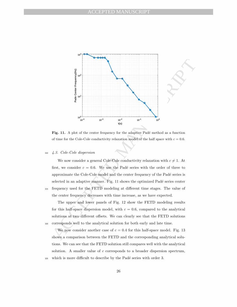
Fig. 11. A plot of the center frequency for the adaptive Pade method as a function

of time for the Cole-Cole conductivity relaxation model of the half space with c = 0.6.

4.3. Cole-Cole dispersion310

We now consider a general Cole-Cole conductivity relaxation with c 6= 1. At

first, we consider c = 0.6. We use the Pade series with the order of three to

approximate the Cole-Cole model and the center frequency of the Pade series is

selected in an adaptive manner. Fig. 11 shows the optimized Pade series center

frequency used for the FETD modeling at different time stages. The value of315

the center frequency decreases with time increase, as we have expected.

The upper and lower panels of Fig. 12 show the FETD modeling results

for this half-space dispersion model, with c = 0.6, compared to the analytical

solutions at two different offsets. We can clearly see that the FETD solutions

corresponds well to the analytical solution for both early and late time.320

We now consider another case of c = 0.4 for this half-space model. Fig. 13

shows a comparison between the FETD and the corresponding analytical solu-

tions. We can see that the FETD solution still compares well with the analytical

solution. A smaller value of c corresponds to a broader dispersion spectrum,

which is more difficult to describe by the Pade series with order 3.325

26

MANUSCRIP

T

ACCEPTED

ACCEPTED MANUSCRIPT

10 -3 10 -2 10 -1

t(s)

10 -2

10 0V

/m

Offset=1000,z=0

AnalyticalFETD

10 -3 10 -2 10 -1

t(s)

10 0

V/m

Offset=2000,z=0

AnalyticalFETD

Fig. 12. A comparison between the analytical and FETD solutions at the offset of

1000 m (upper panel) and 2000 m (lower panel) for the Cole-Cole dispersive half-space

model with c = 0.6.

10-3 10-2 10-1

t(s)

10-4

10-3

10-2

10-1

100

V/m

Offset=2000, z=0

FETDAnalytical

Fig. 13. A comparison between the analytical and FETD solutions at the offset of

2000 m for the Cole-Cole dispersive half-space model with c = 0.4.

27

MANUSCRIP

T

ACCEPTED

ACCEPTED MANUSCRIPT

1000

1000

500

y(m)

0

-500 1000500

x(m)

0-500-1000

-1000

500

z(m

)

3D Model

0

Fig. 14. A 3D model of a conductive cube located within a homogeneous half space.

The blue dots represent the receiver locations, while the red dot on the left indicates

the center position of the electric bipole source.

4.4. 3D model

Now, we consider a 3D model shown in Fig. 14. The source is exactly the

same as in the previous section. This model consists of a half space background

with the conductivity of 10−3 S/m, and a cubic anomaly with the conductivity

of 10−2 S/m. The size of the cube is 500 m × 500 m × 500 m, its center is330

located at a point with coordinates of (0, 0, 500) m. The size of the modeling

domain was 80 km × 80 km × 80 km. The tetrahedral discretization of this

domain contained 270, 553 elements and 319, 029 edges.

For comparison, we also calculated the frequency domain response using the

frequency-domain FEM code (Cai et al., 2017), and the cosine transformation335

was applied to calculate the time-domain response.

In the first numerical test we assumed that there was no IP effect. Fig. 15

shows a comparison between the FETD solution and the frequency domain

transformed solution, at t = 0.1 s, on the earth’s surface. Fig. 16 shows a

28

MANUSCRIP

T

ACCEPTED

ACCEPTED MANUSCRIPT

similar comparison at the receiver located directly above the center of the 3D340

body. We can see that the FETD solution compares well with the frequency

domain transformed solution. The total computation time for this model was

only 10 minutes, with 1416 time steps.

In the next example, we consider the same 3D model, but with the dispersive

conductivity of the cubic body. We first consider a simple Debye relaxation345

model for anomalous conductivity with τ = 0.1 s and η = 0.5.

Fig. 17 shows a comparison between the FETD solution and the frequency

domain transformed solution, at t = 0.1 s for this dispersive model. We can see

that the FETD solution compares well with the frequency domain transformed

result. By comparing this figure with Fig. 15, one can clearly see that the field350

is distorted significantly by the IP effect.

Fig. 18 shows the time domain response, obtained from FETD and cosine

transformation, for this 3D IP model with Debye dispersion at the receiver

which is directly above the center of the 3D body. The total computation time

is around 15 minutes after 1416 time steps. We can see that the computation355

complexity increases after considering the IP effect.

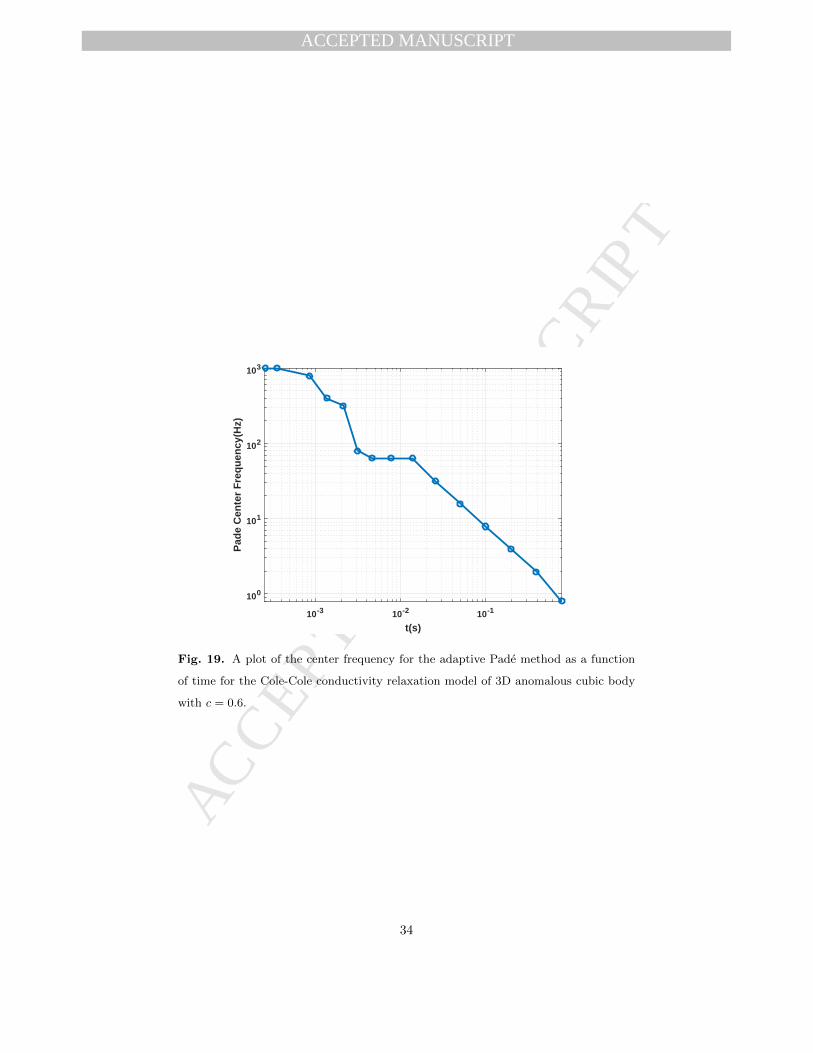
Finally, we consider a general case of the Cole-Cole model with c = 0.6,.

The optimized Pade series with third order and adaptive center frequency were

applied. Fig. 19 shows the center frequency of the adaptive Pade series expansion

at different time stages.360

Fig. 20 shows a comparison between the FETD solution and the frequency

domain transformed result for this model at t = 0.1 s, on the earth’s surface.

Fig. 21 presents the FETD solution and the frequency domain transformed

solution at different time stage for the receiver directly above the center of the

3D body. From these figures, we can see that the FETD solution compares365

well with the frequency-domain transformed result. The computation time was

around 27 minutes after 1416 time steps. For all the above scenarios of this 3D

model, the run time for the frequency-domain finite element code was around 3

hours in the same machine and we have used 51 frequencies uniformly spaced

in logarithmic space from 10−5 Hz to 105 Hz. We want to emphasize that the370

29

MANUSCRIP

T

ACCEPTED

ACCEPTED MANUSCRIPT

FETD, t=0.1 s

-500 0 500 1000x(m)

-1000

-500

0

500

1000

y(m

)

2.5

3

3.5

V/m

×10 -9

Cosine Transform, t=0.1 s

-500 0 500 1000x(m)

-1000

-500

0

500

1000

y(m

)

2.5

3

3.5

V/m

×10 -9

-500 0 500x(m)

2.5

3

3.5

V/m

×10 -9 Ex at y=0

FETDCosine Transform

Fig. 15. A comparison between the FETD solution and the frequency domain trans-

formed solution for the 3D model with no IP effect. The upper and middle panel

shows the map view on the earth’s surface where the arrows represent the direction of

the electric field on the earth’s surface. The lower panel shows a comparison at y = 0

on the earth’s surface.

30

MANUSCRIP

T

ACCEPTED

ACCEPTED MANUSCRIPT

10-3 10-2 10-1 100

time(s)

10-10

10-8

10-6

10-4

V/m

Ex at x=0,y=0

FETDCosine Transform

Fig. 16. A comparison between the FETD solution and the frequency domain trans-

formed solution for the 3D model with no IP effect in the receiver located directly

above the center of the anomaly.

solver for our FETD algorithm is only serial version but the frequency-domain

finite element code we used here adopts the Intel MKL Pardiso solver which is

fully parallelized.

Finally, for comparison, Fig. 22 presents the plots of the electric field com-

puted for the receiver located directly above the 3D body for four different375

scenarios: 1) half-space model with no IP effect; 2) 3D conductivity anomaly

with no IP effect; 3) 3D conductivity anomaly with Debye relaxation; 4) 3D

conductivity anomaly with Cole-Cole relaxation (c = 0.6). By comparing the

electric field for the homogeneous half-space background model and for a model

with 3D anomaly with no IP effect, we can see that the curves are shifted. For380

both Debye and Cole-Cole models of 3D anomalous conductivity, the IP effect

delays the decay of the signal in comparison to the 3D model with no IP effect.

31

MANUSCRIP

T

ACCEPTED

ACCEPTED MANUSCRIPT

FETD, t=0.1 s

-500 0 500 1000x(m)

-1000

-500

0

500

1000

y(m

)

1

2

3

4

5

6

V/m

×10 -7

Consine Transform, t=0.1 s

-500 0 500 1000x(m)

-1000

-500

0

500

1000

y(m

)

1

2

3

4

5

6

V/m

×10 -7

-500 0 500x(m)

-4

-2

0

2

4

6

V/m

×10 -7 Ex at y=0

FETDCosine Transform

Fig. 17. A comparison between the FETD solution and the frequency domain trans-

formed solution for the 3D model with IP effect described by Debye relaxation model.

The upper and middle panel shows the map view on the earth’s surface where the

arrows represent the direction of the electric field on the earth’s surface. The lower

panel shows a comparison at y = 0 on the earth’s surface.

32

MANUSCRIP

T

ACCEPTED

ACCEPTED MANUSCRIPT

10-3 10-2 10-1 100

time(s)

10-10

10-8

10-6

10-4

V/m

Ex at x=0,y=0

FETDCosine Transform

Fig. 18. A comparison between the FETD solution and the frequency domain trans-

formed solution for the 3D model with IP effect described by Debye relaxation model

at the receiver located directly above the center of the anomaly.

5. Conclusions

We have developed an edge-based finite-element time-domain method for

simulating electromagnetic fields in conductive and dispersive medium. We con-385

sider a total field formulation and use unstructured tetrahedral mesh to reduce

the size of the problem. We also use the backward difference, which is uncon-

ditionally stable, for time domain discretization. We adopt time step doubling

methods to gradually increase the step size and reduce the computational ex-

pense. The sparse system of equations is solved using the direct method based390

on a sparse LU decomposition. We have demonstrated that this step doubling

method with direct solver can significantly reduce computation time.

The developed FETD modeling method takes into account the conductivity

dispersion (IP effect) directly in the time domain. We use the Pade series to

approximate the Cole-Cole model, which allows us to approximate the differen-395

tial equation in the time domain with fractional derivatives by the differential

33

MANUSCRIP

T

ACCEPTED

ACCEPTED MANUSCRIPT

10-3 10-2 10-1

t(s)

100

101

102

103

Pad

e C

ente

r F

req

uen

cy(H

z)

Fig. 19. A plot of the center frequency for the adaptive Pade method as a function

of time for the Cole-Cole conductivity relaxation model of 3D anomalous cubic body

with c = 0.6.

34

MANUSCRIP

T

ACCEPTED

ACCEPTED MANUSCRIPT

FETD, t=0.1 s

-500 0 500 1000x(m)

-1000

-500

0

500

1000

y(m

)

0.5

1

1.5

2

2.5

V/m

×10 -7

Cosine Transform, t=0.1 s

-500 0 500 1000x(m)

-1000

-500

0

500

1000

y(m

)

0.5

1

1.5

2

2.5

V/m

×10 -7

-500 0 500x(m)

-20

-10

0

V/m

×10 -8 Ex at y=0

FETDCosine Transform

Fig. 20. A comparison between the FETD solution and the frequency domain trans-

formed solution for the 3D model with IP effect described by Cole-Cole relaxation

model. The upper and middle panel shows the map view on the earth’s surface where

the arrows represent the direction of the electric field on the earth’s surface. The lower

panel shows a comparison at y = 0 on the earth’s surface.

35

MANUSCRIP

T

ACCEPTED

ACCEPTED MANUSCRIPT

10-3 10-2 10-1 100

time(s)

10-7

10-6

10-5

10-4V

/m

Ex at x=0,y=0

FETDCosine Transform

Fig. 21. A comparison between the FETD solution and the frequency domain trans-

formed solution for the 3D model with IP effect described by Cole-Cole relaxation

model at in the receiver located directly above the center of the anomaly.

10-3 10-2 10-1 100

t(s)

10-12

10-10

10-8

10-6

10-4

V/m

Ex at x=0,y=0

Halfspace, No IP3D, No IP3D, IP Debye3D, IP, c=0.6

Fig. 22. The plots of the electric field computed for the receiver located directly

above the 3D body for four different scenarios.

36

MANUSCRIP

T

ACCEPTED

ACCEPTED MANUSCRIPT

equation with integer order. In order to increase the accuracy of the Pade ap-

proximation for a wide time range, we introduced a method of adaptive Pade

series with variable center frequency of the series for early and late time. This

approach increases the accuracy of FETD modeling. We validate the developed400

algorithm using several models with and without the IP effect.

6. Acknowledgement

The authors are thankful to the anonymous reviewers for their valuable

suggestions.

References405

Ascher U. M. and Greif C., 2011. A first course in numerical methods, SIAM,

Philadelphia.

Baker, G.A. and Graves-Morris, P.R., 1996. Pade approximants, Cambridge

University Press, New York.

Cai, H., Hu, X., Li, J., Endo, M. and Xiong, B., 2017. Parallelized 3D CSEM410

modeling using edge-based finite element with total field formulation and

unstructured mesh, Computers & Geosciences, 99, 125-134.

Caputo, M., 1967. Linear model of dissipation whose Q is almost frequency

independent-II, Geophysical Journal Royal Astronomical Society, 13, 529–

539.415

Commer, M. and Newman, G., 2004. A parallel finite-difference approach for

3D transient electromagnetic modeling with galvanic sources, Geophysics, 69,

1192-1202.

Davis, T., 2006. Direct methods for sparse linear systems, SIAM, Philadelphia.

Everett, M.E. and Edwards, R.N., 1993. Transient marine electromagnetics:420

The 2.5-D forward problem, Geophys. J. Int., 113, 545-561.

37

MANUSCRIP

T

ACCEPTED

ACCEPTED MANUSCRIPT

Ge, J., Everett, M.E. and Weiss, C.J., 2012. Fractional diffusion analysis of the

electromagnetic field in fractured media Part I: 2D approach, Geophysics, 77,

WB213-WB218.

Ge, J., Everett, M.E. and Weiss, C.J., 2015. Fractional diffusion analysis of the425

electromagnetic field in fractured mediaPart 2: 3D approach, Geophysics, 80,

E175-E185.

Hallof, P.G. and Yamashita, M., 1990. Induced polarization applications and

case histories, SEG, Tulsa.

Jin, J., 2014. Finite element method in electromagnetics, Third Edition, Wiley-430

IEEE Press, New York.

Knight, J.H., Raiche, A.P., 1982. Transient electromagnetic calculations using

the Gaver-Stehfest inverse Laplace transform method, Geophysics, 47, 47-50.

Li, J., Farquharson, C.G. and Hu, X., 2016. Three effective inverse Laplace

transform algorithms for computing time-domain electromagnetic responses,435

Geophysics, 81, E113-E128.

Luo, Y. and Zhang, G., 1998. Theory and application of spectral induced polar-

ization, SEG, Tulsa.

Maaø, F.A., 2007. Fast finite-difference time-domain modeling for marine-

subsurface electromagnetic problems, Geophysics, 72, A19-A23.440

Marchant, D., Haber, E. and Oldenburg, D.W., 2014. Three-dimensional model-

ing of IP effects in time-domain electromagnetic data, Geophysics, 79, E303-

E314.

Meerschaert, M.M. and Tadjeran, C., 2004. Finite difference approximations for

fractional advectiondispersion flow equations, Journal of Computational and445

Applied Mathematics, 172, 65-77.

Miller, K.S. and Ross, B., 1993. An introduction to the fractional calculus and

fractional differential equations, Wiley-Blackwell,New York.

38

MANUSCRIP

T

ACCEPTED

ACCEPTED MANUSCRIPT

Mulder, W.A., Wirianto, M. and Slob, E.C., 2007. Time-domain modeling of

electromagnetic diffusion with a frequency-domain code, Geophysics, 73, F1-450

F8.

Pelton, W.H., Ward, S.H., Hallof, P.G., Sill, W.R. and Nelson, P.H., 1978.

Mineral discrimination and removal of inductive coupling with multifrequency

IP, Geophysics, 43, 588-609.

Press, W.H., Teukolsky, S.A., Vetterling, W.T. and Flannery, B.P., 1992. Nu-455

merical Recipes in C: The Art of Scientific Computing, Second Edition, Cam-

bridge University Press.

Raiche, A., 1998. Modelling the time-domain response of AEM systems, Explo-

ration Geophysics, 29, 103-106.

Ralph-Uwe, B., Ernst, O.G. and Spitzer, K., 2008. Fast 3-D simulation of tran-460

sient electromagnetic fields by model reduction in the frequency domain using

Krylov subspace projection, Geophys. J. Int., 173, 766-780.

Rekanos, I.T. and Papadopoulos, T.G., 2010. An auxiliary differential equa-

tion method for FDTD modeling of wave propagation in Cole-Cole dispersive

media, IEEE Transactions on Antennas and Propagation, 58, 3666-3674.465

Seigel, H., Nabighian, M., Parasnis, D.S. and Vozoff, K., 2007. The early history

of the induced polarization method, The Leading Edge, 26, 312-321.

Tarasov, A. and Titov, K., 2013. On the use of the ColeCole equations in spectral

induced polarization, Geophys. J. Int., 195, 352-356.

Um, E.S., 2011. Three-dimensional finite-element time-domain modeling of the470

marine controlled-source electromagnetic method, Ph.D dissertation, Stanford

University.

Um, E.S., Harris, J.M. and Alumbaugh, D.L., 2012. An iterative finite element

time-domain method for simulating three-dimensional electromagnetic diffu-

sion in earth, Geophys. J. Int., 190, 871-886.475

39

MANUSCRIP

T

ACCEPTED

ACCEPTED MANUSCRIPT

Wang, T. and Hohmann, G.W., 1993. A finite-difference, time-domain solution

for three-dimensional electromagnetic modeling, Geophysics, 58, 797-809.

Ward, S.H., Hohmann, G.W., 1988. Electromagnetic Theory for Geophysical

Applications, SEG, Tulsa.

Weedon, W.H. and Rappaport, C.M., 1997.A general method for FDTD model-480

ing of wave propagation in arbitrary frequency-dispersive media, IEEE Trans-

actions on Antennas and Propagation, 45, 401-410.

Yee, K.S., 1966. Numerical solution of initial value problems involving Maxwell’s

equationsin isotropic media, IEEE Transactions on Antennas and Propaga-

tion, 14, 302-307.485

Zaslavsky, M., Druskin, V. and Knizhnerman, L., 2011. Solution of 3D time-

domain electromagnetic problems using optimal subspace projection, Geo-

physics, 76, F339-F351.

Zhdanov, M., 2008. Generalized effective-medium theory of induced polariza-

tion, Geophysics, 73, F197-F211.490

Zhdanov, M.S., 2009. Geophysical electromagnetic theory and methods, Elsevier,

Amsterdam.

40

MANUSCRIP

T

ACCEPTED

ACCEPTED MANUSCRIPT

This paper develops a finite element time domain algorithm for geophysical application

We consider a frequency dependent conductivity using Cole-Cole relaxation model

The frequency domain relaxation model is transformed into time domain

We propose the adaptive Padé series to approximate the time domain Cole-Cole

relaxation