final 2003 aqmp appendix v - aqmd.gov
TRANSCRIPT

FINAL 2003 AQMP APPENDIX V
MODELING AND ATTAINMENT DEMONSTRATIONS
AUGUST 2003

SOUTH COAST AIR QUALITY MANAGEMENT DISTRICT
GOVERNING BOARD Chair: WILLIAM A. BURKE, Ed.D. Speaker of the Assembly Appointee Vice Chair: S. ROY WILSON, Ed.D. Supervisor, Fourth District Riverside County Representative MEMBERS: FRED AGUIAR Supervisor, Fourth District San Bernardino County Representative MICHAEL D. ANTONOVICH Supervisor, Fifth District Los Angeles County Representative HAL BERNSON Councilmember, City of Los Angeles Cities Representative, Los Angeles County, Western Region JANE W. CARNEY Senate Rules Committee Appointee WILLIAM CRAYCRAFT Councilmember, City of Mission Viejo Cities Representative, Orange County BEATRICE LAPISTO-KIRTLEY Councilmember, City of Bradbury Cities Representative, Los Angeles County, Eastern Region RONALD O. LOVERIDGE Mayor, City of Riverside Cities Representative, Riverside County LEONARD PAULITZ Councilmember, City of Montclair Cities Representative, San Bernardino County JAMES SILVA Supervisor, Second District Orange County Representative CYNTHIA VERDUGO –PERALTA Governor’s Appointee EXECUTIVE OFFICER BARRY R. WALLERSTEIN, D.Env.


Table of Contents
i
CONTRIBUTORS
Elaine Chang, DrPH Deputy Executive Officer
Planning, Rule Development and Area Sources
Laki Tisopulos, Ph.D., P.E. Assistant Deputy Executive Officer
Planning, Rule Development and Area Sources
Zorik Pirveysian Planning & Rules Manager
Planning, Rule Development and Area Sources
Joseph Cassmassi Satoru Mitsutomi Mark Bassett Chris Nelson Julia Lester Mary Woods Bong-Mann Kim Zhang, Xinqiu
Production Faye Thomas
CALIFORNIA AIR RESOURCES BOARD
Robert Fletcher Division Chief
Technical Support Division
John DaMassa Branch Chief
Cynthia Marvin Branch Chief
Bruce Jackson Sylvia Oey Daniel Chau Joe Calavita Paul Allen Don Johnson
Table of Contents
i
Table of Contents CHAPTER 1 Modeling Overview Introduction........................................................................................................... V - 1- 1 Modeling Methodology ........................................................................................ V - 1- 2
PM10 ........................................................................................................... V - 1- 2 Ozone ......................................................................................................... V - 1- 3
Background..................................................................................... V - 1- 3 Preliminary Future Year Simulation............................................... V - 1- 6 Independent Review ....................................................................... V - 1- 7 Meterological Episode Selection .................................................... V - 1- 10
Carbon Monoxide ...................................................................................... V - 1- 11 Document Organization ........................................................................................ V - 1- 12 CHAPTER 2 Revision to the Federal PM10 Attainment
Demonstration Plan and Visibility Assessment Introduction........................................................................................................... V- 2- 1 Ambient Data Characterization and PTEP ........................................................... V- 2- 2
Annual Average Concentrations................................................................ V- 2- 3 24-Hour Average Concentrations .............................................................. V- 2- 7
Modeling Approach .............................................................................................. V- 2- 9 UAMAERO-LT ......................................................................................... V- 2- 11 UAMAERO-LT Model Inputs .................................................................. V- 2- 12
Modeling Domain........................................................................... V- 2- 13 Boundary, Top and Initial Air Quality Concentrations .................. V- 2- 13 Future Boundary, Top and Initial Air Quality Conditions ............. V- 2- 14 Meteorological Inputs ..................................................................... V- 2- 14 Rain Days........................................................................................ V- 2- 19 9-Cell Averaging ............................................................................ V- 2- 20
Linear Rollback For 24-Hour Average Maximum Concentrations........... V- 2- 20 Emissions Inventory.............................................................................................. V- 2- 21
Emissions Uncertainties............................................................................. V- 2- 22 UAMAERO-LT ......................................................................................... V- 2- 11
Paved Road Dust............................................................................. V- 2- 22 Unpaved Road Dust........................................................................ V- 2- 23 Fugitive Wind Blown Dust............................................................. V- 2- 24 Construction Dust ........................................................................... V- 2- 26
Base-Year Simulations.......................................................................................... V- 2- 28 PM10 Component Species Performance Evaluation for the PTEP Sites............................................................................................................ V- 2- 29

Final 2003 AQMP Appendix V
ii
UAMAERO-LT Component Species Model Performance Evaluation..... V- 2- 30 Annual Average SSI Mass Performance Evaluation ................................. V- 2- 31 1995 UAMAERO-LT Grid-Cell Performance Evaluation........................ V- 2- 46 PM2.5 Component Species Performance Evaluation for the PTEP Sites............................................................................................................ V- 2- 47
Future Air Quality................................................................................................. V- 2- 47 PM10 Control Strategy ............................................................................... V- 2- 48 PM10 in the Year 2006 ............................................................................... V- 2- 49
Annual PM10 By Component Species for the PTEP Sites.............. V- 2- 49 Annual PM10 By Total Mass at the SSI Sites ................................. V- 2- 49 UAMAERO-LT Grid-Level Simulation: 2006 Controlled Emissions ........................................................................................ V- 2- 50 2006 UAMAERO-LT Hot Spot Grid Weight of Evidence Analysis .......................................................................................... V- 2- 51 Maximum 24-Hr Average PM10 ..................................................... V- 2- 56
PM10 in the Year 2010 ............................................................................... V- 2- 57 Annual PM10 ................................................................................... V- 2- 57 Maximum 24-Hr Average PM10 ..................................................... V- 2- 58
PM2.5 in the Year 2010............................................................................... V- 2- 58 Annual PM2.5................................................................................... V- 2- 58 Maximum 24-Hr Average PM2.5 .................................................... V- 2- 59
PM10 in the Year 2010 With Alternative Control Options ........................ V- 2- 60 Conclusions (Particulates) .................................................................................... V- 2- 61 Visibility................................................................................................................ V- 2- 63
Background................................................................................................ V- 2- 63 Visibility Modeling.................................................................................... V- 2- 63 Prior Visibility Modeling Results .............................................................. V- 2- 64 Predicted Future Air Quality...................................................................... V- 2- 66 Future Visibility Projections...................................................................... V- 2- 67
Riverside Future Mean Visibilities................................................. V- 2- 67 Future Light Extinction Budgets at Riverside ................................ V- 2- 69
Conclusions (Visibility) ........................................................................................ V- 2- 70 CHAPTER 3 Revision to the 1997 Ozone Attainment
Demonstration Plan Introduction........................................................................................................... V - 3- 1
Model Selection ......................................................................................... V - 3- 2 Federal 1-Hour Ozone Standard Requirements......................................... V - 3- 3 California Requirements and Population Exposure................................... V - 3- 3
Emissions Summary.............................................................................................. V - 3- 5 Introduction................................................................................................ V - 3- 5 Historical Baseline Emissions ................................................................... V - 3- 6

Table of Contents
iii
Future Baseline Emissions......................................................................... V - 3- 7 Future Controlled Emissions ..................................................................... V - 3- 7
Episode Selection.................................................................................................. V - 3- 7 Southern California Ozone Study (SCOS97) ............................................ V - 3- 9 Statistical Episode Ranking ....................................................................... V - 3- 10 Horie Classification ................................................................................... V - 3- 12 Episodes Compared in the 2002 "Mid-Course" Assessment..................... V - 3- 12
Episode Characterization ...................................................................................... V - 3- 13 Background................................................................................................ V - 3- 13 Synoptic Setting......................................................................................... V - 3- 14 Mesoscale Meteorology............................................................................. V - 3- 15 Air Quality Profile ..................................................................................... V - 3- 16
Modeling Methodology ........................................................................................ V - 3- 17 Model Input Preparation ............................................................................ V - 3- 18
Modeling Domain........................................................................... V - 3- 19 Boundary, Top and Initial Air Quality Concentrations .................. V - 3- 19 Future Boundary, Top and Initial Air Quality Conditions ............. V - 3- 19 Meteorological Scalars ................................................................... V - 3- 20 Meteorological Models ................................................................... V - 3- 21 Temperature Fields ......................................................................... V - 3- 22 Mixing Height Fields...................................................................... V - 3- 23 Gridded Wind Fields....................................................................... V - 3- 27
Model Input Evaluation ............................................................................. V - 3- 29 Temperature Fields ......................................................................... V - 3- 29 Mixing Height Fields...................................................................... V - 3- 29 Wind Fields..................................................................................... V - 3- 39
1997 Base-year perfomance Evaluation ............................................................... V - 3- 40 Statistical Evaluation ................................................................................. V - 3- 41 Graphical Evaluation ................................................................................. V - 3- 45 Effect of Emissions Uncertainties.............................................................. V - 3- 67
Mid-Course Ozone Air Quality Evaluation .......................................................... V - 3- 69 Ozone Air Quality Projections.............................................................................. V - 3- 75
Projection of 2007 Air Quality .................................................................. V - 3- 75 Projection of 2010 Air Quality .................................................................. V - 3- 81 Projection of 8-Hour Average Ozone Air Quality for 2010...................... V – 3-94 Projection of 2010 Air Quality for Alternate Emissions Scenarios........... V – 3-95 Sensitivity Simulations .............................................................................. V – 3-96
Conclusions........................................................................................................... V – 3-96
Final 2003 AQMP Appendix V
iv
CHAPTER 4 Revision to the Federal Carbon Monoxide Attainment Demonstration Plan
Introduction........................................................................................................... V – 4- 1 Carbon Monoxide Emissions................................................................................ V – 4- 2
Introduction................................................................................................ V – 4- 2 Planning Inventory..................................................................................... V – 4- 3
VMT Forecast ................................................................................. V – 4- 3 Emissions Projection ...................................................................... V – 4- 4 Planning Emissions Inventory ........................................................ V – 4- 5
Modeling Methodology ........................................................................................ V – 4- 6 Introduction................................................................................................ V – 4- 6 Regional Modeling Analysis ..................................................................... V – 4- 7 Episode Selection....................................................................................... V – 4- 7 Episode Characterization ........................................................................... V – 4- 8
Synoptic Setting.............................................................................. V – 4- 9 Mesoscale Setting ........................................................................... V – 4- 9 Air Quality Setting.......................................................................... V – 4- 11
Model Selection ......................................................................................... V – 4- 12 Meteorological Modeling and Input Fields .................................... V – 4- 12 Trajectory Analysis......................................................................... V – 4- 14 CAMx Initial and Boundary Conditions ........................................ V – 4- 14 Base Year Emissions ...................................................................... V – 4- 14 Day-of-Week Diurnal Traffic Patterns ........................................... V – 4- 14 Base Year Model Performance....................................................... V – 4- 17
Hot Spot Analysis ...................................................................................... V – 4- 24 Carbon Monoxide Control Strategy...................................................................... V – 4- 26
Contingency Measures............................................................................... V – 4- 26 Future Air Quality Projections.............................................................................. V – 4- 27
Introduction................................................................................................ V – 4- 27 Emissions ................................................................................................... V – 4- 28 Modeling Results ....................................................................................... V – 4- 28
CAMx Regional Simulation ........................................................... V – 4- 28 Linear Rollback of CAMx Simulation Results............................... V – 4- 29
CAL3QHC Modeling Results.................................................................... V – 4- 31 Conclusion ............................................................................................................ V – 4- 32 REFERENCES

CHAPTER 1 MODELING OVERVIEW
Introduction Modeling Methodology Document Organization

Chapter 1 Modeling Overview
V - 1- 1
INTRODUCTION
This appendix to the 2003 AQMP provides the details of the modeling attainment demonstrations presented in Chapter V of the main document. The federal Clean Air Act (CAA) sets forth specific criteria to use air quality simulation modeling techniques to estimate future air quality in areas that do not meet the air quality standards. The Basin is currently designated nonattainment for PM10, ozone, and carbon monoxide. The 2003 modeling attainment demonstrations serve as an update of the 1997 AQMP ozone, PM10 and carbon monoxide plans for the South Coast Air Basin and other portions of the Southeast Desert Modified Nonattainment Area that are under the District’s jurisdiction and were submitted as part of the California SIP. The attainment demonstrations provided in this Plan reflect the updated emissions baseline and future year estimates, new technical information and enhanced air quality modeling techniques and episodes.
Ozone, PM10 and carbon monoxide each have specific air quality modeling requirements that must be met to provide a satisfactory modeling attainment demonstration. Ozone modeling requires the use of a regional analysis using an urban scale air quality simulation model. For particulates, requirements include the use of receptor models and dispersion models to characterize the current and future dispersion of PM10 on a species component level. A photochemical grid model is used to project regional future carbon monoxide (CO) air quality and additional “hot-spot” analyses are required to assess impacts at intersections.
The District’s goal is to develop an integrated control strategy which: 1) ensures that ambient air quality standards for all criteria pollutants are met by the established deadlines in the CAA; and 2) achieves an expeditious rate of reduction towards the state and new federal air quality standards. The overall control strategy is designed so that efforts to achieve the standard for one criteria pollutant do not cause unnecessary deterioration of another. Ozone and PM10 are linked by common precursor emissions and as such the control strategies as well as modeling analyses build upon each other. The District employs a two-step approach to modeling and control strategy development: first assess future PM10 air quality (to meet the 2006 PM10 attainment date) then analyze future 1-hour ozone air quality (to meet the 2010 ozone attainment date). Ozone and PM10 air quality attainment demonstrations analyses under the 2003 AQMP are performed in keeping with this two-step modeling approach. The analyses also consider the future efforts that will be needed to achieve the PM2.5 and 8-hour average ozone standards as they supplant the current air quality standards.
The control strategy to meet federal and state carbon monoxide standards is independent of the PM10/ozone strategy. As previously stated, dispersion modeling and “hot spot” analyses are required for the attainment demonstration. Both analyses are performed in
Final 2003 AQMP Appendix V: Modeling and Attainment Demonstrations
V- 1 - 2
the 2003 AQMP to update the 1997 Revision of the Carbon Monoxide Attainment Demonstration (CO Plan).
The following sections provide a brief overview of the PM10, ozone and carbon monoxide modeling methodologies. In essence, Chapter 1 serves as an addendum to the Modeling Protocol provided as Attachement 1 as it updates the current strategy employed in the 2003 AQMP modeling attainment demonstrations. Chapter 2 presents the detailed PM10 attainment demonstration. Chapter 3 presents the ozone modeling demonstration and Chapter 4 presents the carbon monoxide analysis.
MODELING METHODOLOGY
PM10
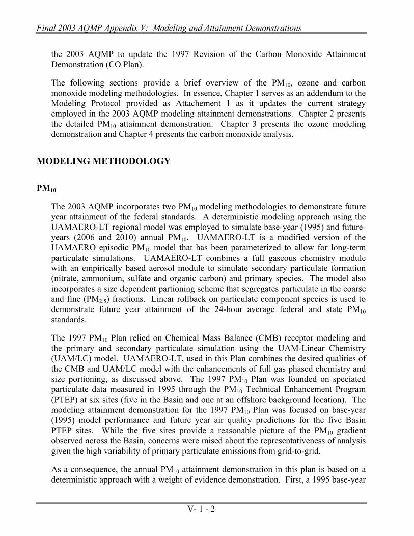
The 2003 AQMP incorporates two PM10 modeling methodologies to demonstrate future year attainment of the federal standards. A deterministic modeling approach using the UAMAERO-LT regional model was employed to simulate base-year (1995) and future-years (2006 and 2010) annual PM10. UAMAERO-LT is a modified version of the UAMAERO episodic PM10 model that has been parameterized to allow for long-term particulate simulations. UAMAERO-LT combines a full gaseous chemistry module with an empirically based aerosol module to simulate secondary particulate formation (nitrate, ammonium, sulfate and organic carbon) and primary species. The model also incorporates a size dependent partioning scheme that segregates particulate in the coarse and fine (PM2.5) fractions. Linear rollback on particulate component species is used to demonstrate future year attainment of the 24-hour average federal and state PM10 standards.
The 1997 PM10 Plan relied on Chemical Mass Balance (CMB) receptor modeling and the primary and secondary particulate simulation using the UAM-Linear Chemistry (UAM/LC) model. UAMAERO-LT, used in this Plan combines the desired qualities of the CMB and UAM/LC model with the enhancements of full gas phased chemistry and size portioning, as discussed above. The 1997 PM10 Plan was founded on speciated particulate data measured in 1995 through the PM10 Technical Enhancement Program (PTEP) at six sites (five in the Basin and one at an offshore background location). The modeling attainment demonstration for the 1997 PM10 Plan was focused on base-year (1995) model performance and future year air quality predictions for the five Basin PTEP sites. While the five sites provide a reasonable picture of the PM10 gradient observed across the Basin, concerns were raised about the representativeness of analysis given the high variability of primary particulate emissions from grid-to-grid.
As a consequence, the annual PM10 attainment demonstration in this plan is based on a deterministic approach with a weight of evidence demonstration. First, a 1995 base-year

Chapter 1 Modeling Overview
V - 1- 3
model simulation is provided for the speciated particulate components and validated through the PTEP data. This base-year simulation is then validated from supplemental annual average Hi-Vol Size Selective Inlet (SSI) PM10 data observed at 18 Basin sites. A grid-cell level analysis of model performance is discussed. The future year annual PM10 attainment demonstration is provided for the particulate component species and total mass at the PTEP sites, as well as the total mass at the SSI locations. As part of the weight of evidence demonstration, the future year grid-cell level simulation is presented and a “hot spot” analysis of individual cells exceeding the federal standard concentration of 50.4 µg/m3 is provided.
Finally, annual and 24-hour average PM2.5 base and future year simulations are presented and discussed in light of the soon-to-be-implemented PM2.5 standard and the future attainment.
Ozone
The CAA requires that ozone nonattainment areas designated as serious and above use a photochemical grid model to demonstrate attainment. The Urban Airshed Model (UAM) with Carbon Bond IV (CB-IV) gaseous chemistry was selected as the modeling tool used in the 2003 AQMP ozone modeling attainment demonstration. UAM is an urban scale, three-dimensional, grid-type, numerical simulation model. It is designed for computing ozone concentrations under short-term, episodic conditions lasting one to three days. UAM simulations have been incorporated as the basis of the Basin ozone modeling attainment demonstrations since the 1989 AQMP. On the date of the release of the Draft 2003 AQMP, UAM was the photochemical model, recommended by the U.S. EPA guidance (40 CFR Part 51, Appendix W). On April 15, 2003, the final revisons to Appendix W were published in the Federal Register. Revised Appendix W removed UAM as the sole recommended model by EPA for ozone analysis, and in its place did not name a successor. Revised Appendix W promotes the use of models employing state-of-the-art advances in science.
Background
In 1999, at the inception of the 2003 AQMP modeling effort, the Modeling Staffs of the District and California Air Resources Board jointly developed a Modeling Protocol to layout a design for evaluating several meteorological, regional air quality and chemical models using the newly acquired Southern California Air Quality Study (SCOS97) data set. The Modeling Protocol was distributed to the SCOS97 Working Groups and Stakeholders. (EPA is a member of the SCOS97 Stakeholders).
The proposed scope of the modeling effort was extensive. The ultimate goal of joint effort was to accurately simulate multiple meteorological air quality episodes (meeting EPA’s model performance criteria) with the greatest combination of modeling tools not

Final 2003 AQMP Appendix V: Modeling and Attainment Demonstrations
V- 1 - 4
only for the AQMP, but for interbasin pollutant transport and future 8-hour average ozone impacts. The modeling effort planned to take advantage of upgrades made to the emissions inventory in several areas, most notably, the mobile source categories (on and off-road). In total, seven air quality models, three meteorological model combinations and three chemistry packages, selected through the modeling protocol were evaluated to some or full extent. Table 1-1 lists the different model platforms and chemical mechanisms assessed.
Table 1-1 Air Quality and Meteorological Modeling Platforms and Chemical Mechanisms
Evaluated for the 2003 AQMP
Air Quality Models Meteorological Models Chemistry Mechanisms
UAM MM5 CB-IV
UAM-FCM CALMET SAPRC99
CALGRID MM5/CALMET (Hybrid) TOX
CAMx
CMAQ
MAQSIP
SAQM
As the modeling efforts began to take shape, the District and ARB staff divided the work effort to maximize productivity. The first tasks involved reviewing the SCOS97 meteorological data and meteorological modeling tools. The original timetable was designed to provide working meteorological air quality episodes for a scheduled 2000 draft AQMP. Four SCOS97 meteorological episodes and one meteorological episode from July, 1998 (where a significant portion of the upper air monitoring network remained in southern California) were identified as candidates. The August 3-7, 1997 meteorological episode was selected as the primary ozone episode. August 5th (the Basin's 1997 2nd maximum ozone day) and August 6th (an eddy circulation day with transport to Ventura County, Antelope Valley and the Mojave Desert) were selected as episode simulation days for the analysis. (The UAM simulation was started late on August 3rd, a Sunday, and as consequence there were concerns about the accuracy of the weekend inventory used on the first day and the impact that the inventory uncertainty

Chapter 1 Modeling Overview
V - 1- 5
had on the transition to a weekday simulation. In addition, since the simulation "ramp-up" began late in the day on the 3rd, there were concerns that the initial conditions may have been carried late into the day of the 4th).
Extensive review of the meteorological data was conducted through the SCOS97 Meteorological Working Group and contracted quality assurance programs (NOAA and STI). Further work by ARB emissions staff and the SCOS97 Emissions Working Group resulted in significant improvements in aircraft, shipping and biogenic emission inventories. Unfortunately, the final mobile source emission inventories from the on and off-road models (EMFAC2002 and Off-Road), were not available until November 2002. Final model validation on the meteorological episodes did not commence until winter of 2002.
Through the course of model development, the progress made and methodologies evaluated were routinely presented to the Scientific, Technical and Peer Modeling Advisory Group of the AQMP Advisory Committee. In addition, independent peer reviews of the work in progress were conducted by Dr. Robert Harley of the University of California at Berkeley and Dr. William Carter of the University of California at Riverside. The mid-course critique was provided to the ARB and District modeling staffs.
By the time the emissions were frozen, the air quality models and chemistry packages still being considered for use in the ozone modeling attainment demonstration reduced to the UAM with CB-IV chemistry, the California Photochemical Grid Model (CALGRID) using CB-IV and SAPRC99 chemistry, and the Comprehensive Air Quality Model with Extensions (CAMx), with CB-IV and SAPRC99 chemistry. CALGRID is a regional scale, three dimensional, grid type model that embodies several enhancements in layer structure, advection and dispersion schemes not found in UAM. State-of-the science advances in modeling technology present in CAMx take advantage of the direct coupling with the non-hydrostatic MM5 primitive equation meteorological model. The SAPRC99 chemistry reflects the state of the science in chemical mechanisms with its enhanced treatment of reactivity and interaction of additional chemical species. Preliminary results of the model performance evaluation for the August 1997 episode at the key ozone receptor areas in the Basin indicated that all five model/chemistry combinations achieved the minimum requirements specified in EPA modeling guidance for use in the attainment demonstration. Specifically, UAM had the best performance overall in simulating the unpaired peak concentration, essentially matching the August 5, 1997 observed concentration of 188 ppb. CALGRID and CAMx performed better in recreating the timing and location of the observed peak ozone concentration. Use of the SAPRC99 chemistry in CALGRID and CAMx increased model performance in simulating the unpaired peak concentration compared with the CB-IV chemistry. However, both models continued to under predict, failing to predict the peak concentration within ten percent of the observed concentration.

Final 2003 AQMP Appendix V: Modeling and Attainment Demonstrations
V- 1 - 6
Preliminary Future Year Simulations
Three of the five model-chemistry combinations were run to simulate attainment of the ozone standard in 2010 with the oxides of nitrogen (NOx) emissions held at the final 1997 AQMP level. The preliminary results varied significantly in the determination of the volatile organic compound (VOC) carrying capacities required to meet attainment criteria. (CAMx/CB-IV and CALDRID/CB-IV under predicted unpaired peak concentrations greatest in the base year simulation and in-turn were excluded from future consideration). The 2010 emissions were considered preliminary since they represent across the board reductions from the final base-year totals and did not reflect implementation of a specific control strategy. CAMx/SAPRC99 which had the lowest unpaired predicted to observed peak ratio projected the highest (VOC) carrying capacity of 560 TPD. CALGRID/SAPRC99 which had the second best unpaired predicted to observed peak ratio predicted a VOC carrying capacity of 420 TPD, essentially equivalent to the VOC established by the 1997 AQMP. The 330 TPD carrying capacity derived by UAM was roughly equivalent to that defined by the 1991 and 1994 AQMP’s.
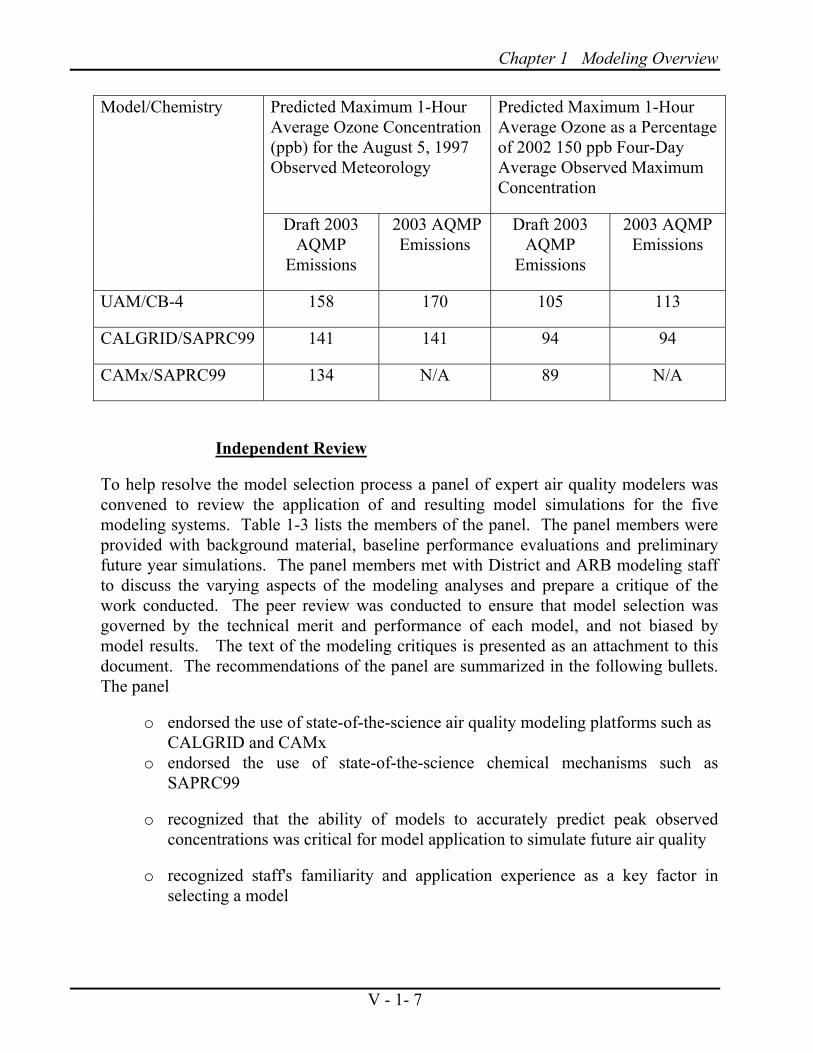
With the large spread in projected carrying capacity not resolved, an independent test of model performance was run to try and refine the model selection process. Emissions for 2002 were generated and simulated by the three modeling systems. The process was essentially a “mid course” analysis that is recommended in EPA’s modeling guidance as part of a weight of evidence analysis to support model validation and acceptance. Average ozone air quality from four days during the summer of 2002 having similar meteorological profiles to the primary episode day (August 5, 1997) was used to validate predictions. The days in 2002 were ranked within a range of ± 6 out of 2557 cases based on a statistical analysis (described in Chapter 3). The four-day average concentration was 150 ppb but included the observed annual Basin maximum one hour average concentration of 169 ppb. The results of the “mid-course” simulations are presented in Table 1-2 for both the Draft and 2003 AQMP emissions inventories. Revisions to the 2002 emissions inventory following the release of the Draft 2003 AQMP resulted in an increase of 24 TPD of VOC in the Basin and a reduction of 6 TPD of NOx. The analysis shows that the UAM performed best on this independent test for the Draft 2003 inventory. When VOC emissions were increased for the final inventory, UAM slightly over predicted the four day average but recreated the peak concentration observed in 2002. Even with the additional VOC emissions, CALGRID was not able to produce additional ozone. Note, CAMx was not run using the 2003 AQMP emissions for the “mid-course” analysis.
Table 1-2 2002 "Mid-Course" Ozone Simulation
Chapter 1 Modeling Overview
V - 1- 7
Predicted Maximum 1-Hour Average Ozone Concentration (ppb) for the August 5, 1997 Observed Meteorology
Predicted Maximum 1-Hour Average Ozone as a Percentage of 2002 150 ppb Four-Day Average Observed Maximum Concentration
Model/Chemistry
Draft 2003 AQMP
Emissions
2003 AQMP Emissions
Draft 2003 AQMP
Emissions
2003 AQMP Emissions
UAM/CB-4 158 170 105 113
CALGRID/SAPRC99 141 141 94 94
CAMx/SAPRC99 134 N/A 89 N/A
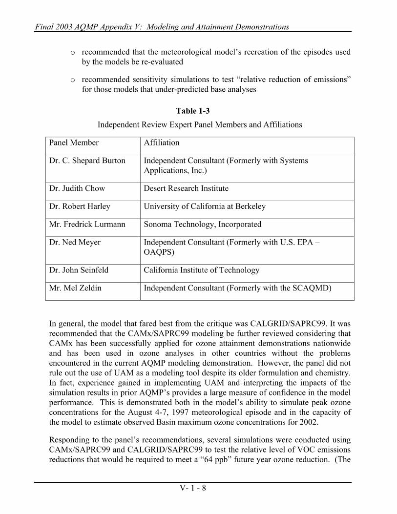
Independent Review
To help resolve the model selection process a panel of expert air quality modelers was convened to review the application of and resulting model simulations for the five modeling systems. Table 1-3 lists the members of the panel. The panel members were provided with background material, baseline performance evaluations and preliminary future year simulations. The panel members met with District and ARB modeling staff to discuss the varying aspects of the modeling analyses and prepare a critique of the work conducted. The peer review was conducted to ensure that model selection was governed by the technical merit and performance of each model, and not biased by model results. The text of the modeling critiques is presented as an attachment to this document. The recommendations of the panel are summarized in the following bullets. The panel
o endorsed the use of state-of-the-science air quality modeling platforms such as CALGRID and CAMx
o endorsed the use of state-of-the-science chemical mechanisms such as SAPRC99
o recognized that the ability of models to accurately predict peak observed concentrations was critical for model application to simulate future air quality
o recognized staff's familiarity and application experience as a key factor in selecting a model
Final 2003 AQMP Appendix V: Modeling and Attainment Demonstrations
V- 1 - 8
o recommended that the meteorological model’s recreation of the episodes used by the models be re-evaluated
o recommended sensitivity simulations to test “relative reduction of emissions” for those models that under-predicted base analyses
Table 1-3 Independent Review Expert Panel Members and Affiliations
Panel Member Affiliation
Dr. C. Shepard Burton Independent Consultant (Formerly with Systems Applications, Inc.)
Dr. Judith Chow Desert Research Institute
Dr. Robert Harley University of California at Berkeley
Mr. Fredrick Lurmann Sonoma Technology, Incorporated
Dr. Ned Meyer Independent Consultant (Formerly with U.S. EPA – OAQPS)
Dr. John Seinfeld California Institute of Technology
Mr. Mel Zeldin Independent Consultant (Formerly with the SCAQMD)
In general, the model that fared best from the critique was CALGRID/SAPRC99. It was recommended that the CAMx/SAPRC99 modeling be further reviewed considering that CAMx has been successfully applied for ozone attainment demonstrations nationwide and has been used in ozone analyses in other countries without the problems encountered in the current AQMP modeling demonstration. However, the panel did not rule out the use of UAM as a modeling tool despite its older formulation and chemistry. In fact, experience gained in implementing UAM and interpreting the impacts of the simulation results in prior AQMP’s provides a large measure of confidence in the model performance. This is demonstrated both in the model’s ability to simulate peak ozone concentrations for the August 4-7, 1997 meteorological episode and in the capacity of the model to estimate observed Basin maximum ozone concentrations for 2002.
Responding to the panel’s recommendations, several simulations were conducted using CAMx/SAPRC99 and CALGRID/SAPRC99 to test the relative level of VOC emissions reductions that would be required to meet a “64 ppb” future year ozone reduction. (The

Chapter 1 Modeling Overview
V - 1- 9
64 ppb level represents the difference between the August 5, 1997 observed maximum 1-hour average concentration and the federal standard of 124 ppb). When the relative reduction techniques were applied to the CALGRID/SAPRC99 and CAMx/SAPRC99 model runs, the projected VOC carrying capacities closed the gap with the UAM carrying capacity. Yet the CAMx runs produced the highest VOC carrying capacities and given the base year and “mid course” correction simulations being significantly under predicted, continued use of the model for the 2003 AQMP attainment demonstration was ruled out.
Modifications were made to several meteorological fields to attempt to increase the CALGRID/SAPRC99 base-year peak ozone prediction. These actions included adjustments to the vertical mixing profiles and smoothing of meteorological field parameters. These adjustments and simulating with the final 2003 AQMP emissions resulted in a nominal increase in base-year performance where the peak predicted ratio increased to 0.89 (a maximum predicted concentration of 167 ppb). Additional modifications were made to the methodology used to roll back future-year boundary conditions. CALGRID/SAPRC99 was extensively simulated using the final emissions control strategy. The initial results of the simulations indicated that the SAPRC99 mechanism was very “stiff” and not responsive to reductions of VOC at targeted levels of NOx (approximately 541 TPD). One area of concern was the impact of biogenic emissions, both in emissions tonnage on the primary modeling day and in the complexities in the speciation of the biogenic volatile organic compounds for the SAPRC99 chemical mechanism. With the uncertainties of the response of the chemical mechanism to the proposed control strategy, it was determined that the CALGRID/SAPRC99 mechanism needed further evaluation.
Sensitivity analyses, including the use of the ozone apportionment tool, were conducted for both CALGRID/SAPRC99 and UAM to test the contribution of biogenic emissions to the 2010 predicted ozone. The sensitivity analyses indicated that the biogenic emissions were contributing about 30 percent to the peak predicted concentration, regardless of modeling platform. While relative weight of the biogenic emissions to the total ozone formation was considered “high” the results for the two models were similar, despite the differences in the chemical mechanisms and the SAPRC99 speciation profile.
The CALGRID/SAPRAC99 2010 predicted peak ozone concentration for the 2003 AQMP emissions and the primary control scenario (modeling remaining emissions of 314 TPD of VOC and 519 TPD of NOx), valued 117 ppb. As with the preliminary simulations, the sensitivity to reductions in VOC at the set level of NOx emissions was low, translating to an approximate 16 TPD of VOC reduction for each ppb of ozone reduced. (This approximate ratio was demonstrated for several NOx thresholds through modeling conducted by the ARB using across the board emissions reductions). Scaling the federal standard by the ratio that CALGRID/SAPRAC99 under predicted the base-year ozone peak provides an alternate equivalent standard of 110 ppb. This is a

Final 2003 AQMP Appendix V: Modeling and Attainment Demonstrations
V- 1 - 10
modified version of the panel’s recommendation to test the relative level of VOC reduction needed to account for under prediction in the base-year simulation. If this scaled standard were the target for emissions reductions, significant additional reductions of VOC emissions would be necessary.
UAM was selected as the primary modeling tool to determine the Basin emissions carrying capacities for the 2003 AQMP. The primary reasons for selecting UAM are:
o UAM predicted the unpaired peak concentration best in the validation
o UAM performed the best in the “mid-course” correction simulation
o Staff has extensive experience with the model application
The AQMP process is committed to continue to evaluate CALGRID and CAMx (using CB-IV and SAPRC99 chemistry). As with CALGRID, the modeling staff is continuing to evaluate the CAMx performance to bring it in line with the other two models. The UAM will remain as the primary modeling tool for the 2003 AQMP. A technical report discussing the CALGRID simulations analysis is provided as Attachment–7 to AQMP Appendix V.
Meteorological Episode Selection
The UAM ozone attainment demonstration was based on two meteorological episodes: August 5-6, 1997 and August 27-28, 1987. Model input data supporting the UAM simulations were derived from intensive field monitoring that occurred during the 1997 Southern California Ozone Study (SCOS97) and the 1987 South California Air Quality Study SCAQS. The SCOS97 study benefited from state-of-the art upper air wind and temperature monitoring and recently developed advances in particulate and oxides of nitrogen sampling technology. The SCAQS field program was the state-of-science in 1987, however the extent and sophistication of field monitoring was now ten years older than that used in SCOS97. US EPA requires that meteorological episodes and the data supporting the modeling attainment demonstration be no more than ten years old for this very reason.
The August 5-6, 1997 episode was selected as the primary modeling episode. The August episode was the Basin second maximum ozone for 1997, and the 188 ppb is equivalent to the current ozone design value (185 ppb). As part of the episode selection process, all days during the months May through October covering the period 1981 through 2002 were ranked by ozone meteorological episode potential. The statistical empirical analysis (described further in Chapter 3) is equivalent to that itemized by Cox and Chu and the 1996 revisions to EPA Ozone Modeling Guidance. Using the ranking
Chapter 1 Modeling Overview
V - 1- 11
system, the August 1997 episode was identified as being more severe than the August 1987 episode. The 1987 SCAQS episode however, was retained for the analysis as a measure of consistency between modeling attainment demonstrations.
Overall, the days represented by the two meteorological episodes fall into the “high-ozone” category. While it is desirable to have a distribution of different meteorological episodes to study, over the past five years, the days exceeding the ozone standard have become more and more restricted to the high ozone potential day.
Two additional SCOS97 meteorological episodes were considered for potential simulation: (1) September 28-29, 1997, a weekend episode and (2) October 31-November 1, 1997. Model performance for the September episode did not meet EPA criteria and it was excluded from this analysis. The October-November episode is being used for the current 2003 CO attainment demonstration. One additional episode was considered, July 14-18, 1998, however, that episode represented meteorological conditions that are severe and rare, occurring less than once in a four year period. The statistical ranking of the episode days confirmed the severity of the July 14-18, 1998 meteorological episode (i.e. 99.8th percentile of the past 22-years). As a consequence, that episode was excluded from the attainment demonstration.
The meteorological and air quality field data monitored during the August 1997 episode has been extensively analyzed over a two year period by the SCOS97 Meteorological Working Group as well as NOAA and contracted air quality consultants. The data has undergone extensive quality assurance and the ensuing meteorological model input developed from the data has been evaluated using the state-of-science meteorological models.
Carbon Monoxide
CAMx, with CB-IV chemistry and the CAL3QHC roadway intersection "Hot Spot" model were the modeling tools used in the 2003 AQMP carbon monoxide modeling attainment demonstration. In the 1997 CO Plan, the regional dispersion modeling was conducted using UAM as a modeling platform. CAMx, with its fixed layer height vertical structure was selected for the current application because it is more suited to address ground level carbon monoxide impacts from tailpipe emissions and low level wind drift of regional carbon monoxide background concentrations. CAMx was run with the CB-IV chemistry; however, carbon monoxide is essentially inert in the fall nighttime application. As a consequence, the modeling effort was focused towards regional transport and local dispersion.
A new modeling episode was introduced for the modeling attainment demonstration, October 31, - November 1, 1997. The meteorological episode was the final SCOS97 intensive monitoring of the active program and benefited from the extensive field

Final 2003 AQMP Appendix V: Modeling and Attainment Demonstrations
V- 1 - 12
monitoring in place. Three specific aspects of the episode are important to note: First, the episode took place on a weekend beginning on Friday night and carrying through Saturday morning. Second, the episode began on Halloween night and it is difficult to estimate the local traffic impact resulting from the holiday activities. Finally, while not as severe an episode as was used in the previous AQMP's, the October 31, - November 1, 1997 episode was the second most severe since Phase II fuel reformulation was implemented and has not been surpassed in concentration since its occurrence.
The 2003 CO Plan will serve as a replacement for the 1997 CO Plan that lapsed in 2000. Over the two year period since the attainment demonstration lapsed the Basin has met the criteria for attainment of the federal 8-hour average carbon monoxide standard. (The Basin did not exceed the federal 8-hour average carbon monoxide standard in 2001 and exceeded the standard only once in 2002). Thus, the 2003 CO attainment demonstration will provide the basis for a future maintenance plan for the Basin pending submission of a petition for redesignation of attainment status.
DOCUMENT ORGANIZATION
This document provides the federal attainment demonstrations for PM10, ozone and carbon monoxide. Chapter 2 provides the PM10 attainment demonstration to meet the 2006 attainment date. The discussion includes future year (2010) particulate impacts for both PM10 and PM2.5. Chapter 3 presents the ozone attainment demonstration based on the UAM modeling analyses. The ozone analysis includes a characterization of the episode, base-year modeling performance, and future year attainment for two control strategies. As with the particulate analysis, a series of alternative emissions simulations are presented to test the sensitivity of the proposed control strategy. Chapter 4 presents the CO attainment demonstration and it includes a detailed analysis of the emissions, and observed meteorological episode. The list of references cited in the document follows.
Table 1-4 lists the Appendices and Attachments to this document.

Chapter 1 Modeling Overview
V - 1- 13
Table 1-4 Appendices and Attachments
Appendix/Attachment Description
Appendix A Model Performance Statistics and Graphical Evaluation
Attachment-1 ARB/District Modeling Protocol
Attachment-2 The Critiques of the expert Researcher's panel
Attachment-3 Mid-term Critiques of the Independent Reviewers
Attachment-4 CEPA Source Level Emissions Reduction Summary for 2006: Annual Average Inventory
Attachment-5 CEPA Source Level Emissions Reduction Summary for 2010: Annual Average Inventory
Attachment-6 CEPA Source Level Emissions Reduction Summary for 2010: Planning Inventory
Attachment 7 Technical Report: CALGRID Ozone Simulations

CHAPTER 2 REVISION TO THE FEDERAL PM10 ATTAINMENT DEMONSTRATION PLAN AND VISIBILITY ASSESSMENT
Introduction
Ambient Data Characterization and PTEP
Modeling Approach
Emissions Inventory
Base-Year Simulations
Future Air Quality
Conclusions (Particulates)
Visibility
Conclusions (Visibility)


Chapter 2 PM10 Attainment and Visibility
V - 2- 1
INTRODUCTION
In the 1997 AQMP the Urban Airshed Model with Linear Chemistry (UAM/LC) [Kumar, et al, 1995] modeling system together with the Chemical Mass Balance (CMB) receptor model provided the platforms for simulating the base and future year PM10 concentrations for the Basin. EPA guidance on PM modeling requires the use of a dispersion model in combination with a receptor model for attainment demonstrations. The UAM/LC modeling system is a multi layered, Eularian grid model with a parameterized linear chemistry used to simulate secondary aerosol formation in the atmosphere. UAM/LC was used to simulate annual primary and selected secondary aerosol components (ammonium, sulfates and nitrates) for the model year 1995. The CMB receptor model used a South Coast Air Basin specific emissions source profile to estimate secondary organic components. The model simulations were supported by corroborating analyses including a modified speciated rollback calculation, and the use of an episodic PM10 model, UAM-AERO in conjunction with a statistical analysis to extrapolate the episodic simulation for an annual application. A detailed description of the modeling approach, tools used and data used in the analyses is presented in Chapter 2 of Appendix V to the 1997 AQMP.
The 1997 AQMP focused on simulating annual particulate for five key sites in the Basin (Rubidoux, Fontana, Diamond Bar, Anaheim and Central Los Angeles) where enhanced field measurements were conducted during 1995 through the PM10 Technical Enhancement Program (PTEP). The PTEP data provided comprehensive analysis of the component species of both the fine and coarse partitions of particulate samples. The PTEP field program captured particulate data on 222 days in 1995, with a focus towards the fall and early winter months when high values of secondary components, in particular nitrate are often observed. The particulate profile has been roughly grouped into six general components including the ions ammonium, nitrate, and sulfate; organic carbon, elemental carbon and primary matter (others). The PTEP program is described in detail in Chapter 2 of Appendix V of the 1997 AQMP.
Subsequent to the submission of the 1997 AQMP PM10 plan, efforts were undertaken to enhance the annual PM simulation capability and extend the analyses to PM2.5. Desired components of the UAM/LC and UAM-AERO models were merged and enhanced by incorporating a parameterized aerosol chemistry module into the UAM-Flexible Chemistry Model (UAM-FCM) [Kumar, et al, 1995] with PM2.5 partitioning. The resulting UAMAERO-LT (LT-long term) model provided a more robust, stand-alone platform for primary and secondary particulate simulation including secondary organic species. The UAMAERO-LT is described in more detail in a following section.

Final 2003 AQMP Appendix V: Modeling and Attainment Demonstrations
V - 2- 2
For the 2003 AQMP, PM10 and PM2.5 modeling was conducted using the UAMAERO-LT model for the 1995 base year. Simulations were conducted for the same modeling gridded domain as the 1997 AQMP using a modified version of the 1995 base year meteorological input data and 5-layers (compared with two used for the UAM/LC simulation). The emissions inventories have been significantly upgraded to address enhancements to the on-road and off-road mobile source inventories through EMFAC2002. Additional updates in the point and area source inventories and the ammonia inventory have been added to the simulation.
The 1997 AQMP merged the results of receptor and dispersion modeling techniques to simulate annual and 24-hour averaged maximum concentrations of PM10 to demonstrate future year attainment. The 2003 AQMP relies on a deterministic approach using the UAMAERO-LT to simulate base and future year annual average PM10 and PM2.5. While the emissions inventory is specified for weekdays, Saturdays and Sundays, and is temperature corrected for each month, short-term episodic modeling using this inventory is inappropriate to estimate maximum 24-hour PM10 and PM2.5 concentrations for the Basin. Linear rollback on the particulate component species is used to estimate future maximum 24-hour average particulate concentrations. In addition, a weight of evidence discussion is provided to address uncertainties in the analysis and provide support that the regional modeling is demonstrating future year attainment of the particulate standard.
The following sections briefly describe the 1995 air quality profile and PTEP, address the characterization of the UAMAERO-LT modeling platform, modeling domain, meteorological fields, boundary and initial conditions, and emissions uncertainties. The results of the base year simulation are compared to observations to quantify model performance. The future base year and controlled emissions simulations are presented to demonstrate attainment of the annual and 24-hour maximum PM10 standards in 2006. Additional future year (2010) simulations are presented to demonstrate progress made towards attaining the new PM2.5 standard (date yet to be determined) and the additional emissions reductions that will be needed to achieve that goal. Finally, the analysis addresses the post 2010 emissions reductions that will be needed to attain the recently revised California PM10 and PM2.5 standards.
AMBIENT DATA CHARACTERIZATION AND PTEP
The 1995 ambient particulate air quality setting in the Basin and the PTEP monitoring program are extensively characterized in Appendix V of the 1997 AQMP. This section provides a brief summary of the PTEP data analysis and an expanded assessment of the SSI Hi-Vol data measured at the District monitoring sites. Figure 2-1 shows the locations of both the PTEP sites and the District’s network of SSI Hi-Vol monitoring locations.

Chapter 2 PM10 Attainment and Visibility
V - 2- 3
FIGURE 2-1 Particulate Monitoring Network: SSI Hi-Vol and PTEP Enhanced Monitoring Network in Bold (San Nicholas Island not shown)
Annual Average Concentrations
Figures 2-2 and 2-3 depict the relative contributions of the major components of particulate to the annual average PM10 and PM2.5 measured at each of the PTEP sites. In the figures, the sites are presented in a west to east orientation whereby the offshore background site SANI (San Nicholas Island) is on the left of the figure and Rubidoux farthest right. This orientation is aligned with wind driven mass transport in the Basin. In general, the west Basin stations of ANAH (Anaheim), CELA (Central Los Angeles) and DBAR (Diamond Bar) are relatively consistent in percentage component mass with CELA exhibiting higher nominally nitrate, and organic carbon fractions. In contrast, concentrations of nitrate, organic carbon and others (including wind blown dust, and primary geological material) are dominant at the eastern Basin sites of FONT (Fontana) and RIVR (Rubidoux) that are subjected to transport and enhanced secondary aerosol formation due to ammonia emissions from upwind dairy and farming operations in those areas.

Final 2003 AQMP Appendix V: Modeling and Attainment Demonstrations
V - 2- 4
The PM2.5 component analysis shows a similar pattern to that of PM10 however the percentage contributions are adjusted to reflect the near absence of the primary category (others) in the fine particulate portion of the distribution. In general, PM2.5 total mass is more associated with combustion related sources and secondary aerosol formation.
It is important to note that PTEP sampling took place on 222 days during 1995. The District’s ambient SSI sampling program operated on approximately 61 days that year. PTEP sampling was conducted at all six sites on a one-day-in-six schedule during the first quarter of 1995. The sampling frequency was increased to one-day-in-three during the second quarter of 1995, and during the second half of 1995, sampling frequency was increased to every day. Only San Nicolas Island (due to logistical limitations) remained on a one-day-in-six sampling schedule. Table 2-1 provides a comparison of the annual average concentrations measured at the PTEP sites and the co-located SSI data sampled for a routine one-day-in-six schedule. When all data is analyzed, with the exception of Anaheim, the PTEP annual average concentration was higher than the corresponding SSI annual average. When the data is paired by SSI sampling day, the annual averages agree well at all sites.
FIGURE 2-2 1995 PTEP Annual Average Speciated PM10 Concentrations
0
10
20
30
40
50
60
70
80
SANI ANAH CELA DBAR FONT RUBX
SO4 NO3 NH4 OC EC Na Cl Others
µg/m3

Chapter 2 PM10 Attainment and Visibility
V - 2- 5
FIGURE 2-3 1995 PTEP Annual Average Speciated PM2.5 Concentrations
Table 2-1
Comparison of the PTEP and SSI 1995 Annual Average PM10 Concentrations
PTEP SSI Paired PTEP/SSI Location Annual Average (µg/m3)
Number of Samples
Annual Average (µg/m3)
Number of Samples
Annual Average (µg/m3)
Number of Samples
Anaheim
42.2 141 43.5 60 42.3 53
Central Los Angeles
52.0 141 42.8 60 50.1 55
Diamond Bar
46.5 140 46.0 61 46.8 51
Fontana
66.8 137 61.0 61 64.1 52
Rubidoux
78.0 157 69.0 61 74.0 56
The federal PM10 annual standard is based on the SSI sampler data measured on the one-day-in-six schedule. While the sampling frequency of PTEP was greater than the SSI, there were periods early in 1995 when only the SSI analysis was available. As a result, the PTEP data was not directly used for annual model validation.
05
1015202530354045
SANI ANAH CELA DBAR FONT RUBX
SO4 NO3 NH4 OC EC Na Cl Others
µg/m3

Final 2003 AQMP Appendix V: Modeling and Attainment Demonstrations
V - 2- 6
Instead, the PTEP data was used to apportion the SSI measured annual arithmetic mean total mass (e.g. 69 µg/m3 at RIVR) into the major particulate component species. Table 2-2 (repeated from 1997 AQMP Appendix V) lists percentage contributions of the individual species for each PTEP site based on the annual sampling program. For the UAMAERO-LT modeling validation and attainment demonstration, the percentage mass contributions of the major particulate species to the total mass analyzed from the site specific PTEP data are multiplied by the corresponding SSI annual average mass concentrations at the five SSI sites to estimate annual averages of the particulate component species. Table 2-3 summarizes the component mass of the apportioned SSI PM10 data.
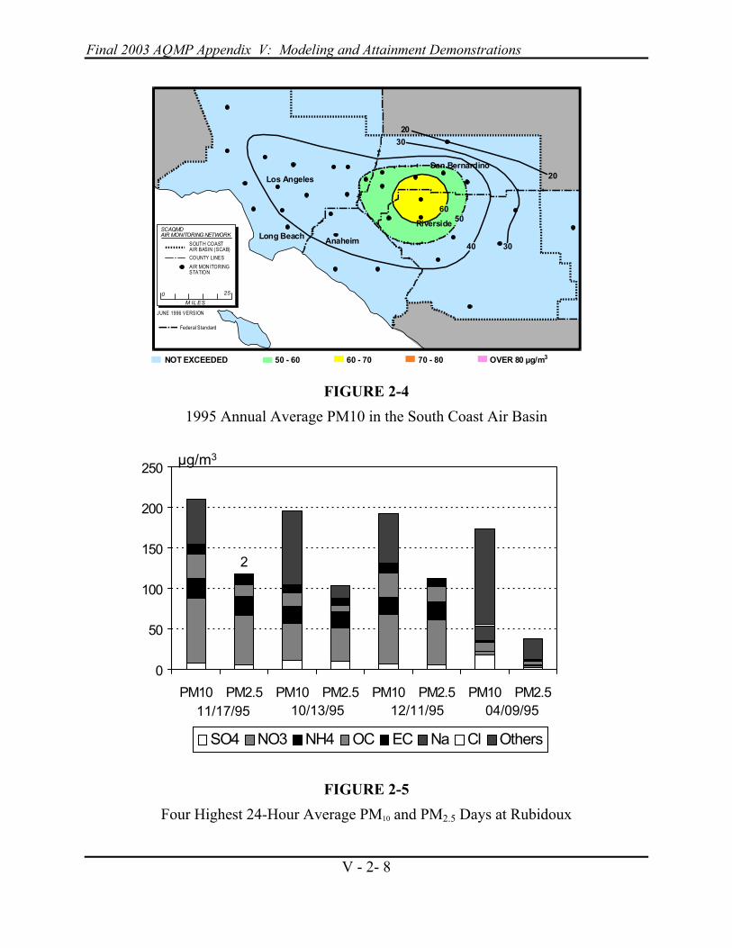
Figure 2-4 shows the Basin-wide distribution of annual arithmetic mean PM10 concentrations for 1995. The highest concentrations are located in the eastern Basin at Rubidoux and Fontana with annual average concentrations above 50.4 backing into parts of Orange and Los Angeles Counties. The gradation of particulate concentrations that is evident in the figure is substantiated by annual average concentrations measured at the District’s SSI monitors presented in Table 2-4. The SSI data and the analyzed spatial distribution provide an enhanced basis for estimating the base-year UAMAERO-LT simulation performance.
TABLE 2-2 Annual Average PM10 Species Concentrations at the Five Basin PTEP Sites
Anaheim Downtown LA Diamond Bar Fontana Rubidoux Component
Mass % Mass % Mass % Mass % Mass %
PM10 mass 42.16 51.97 46.52 66.84 77.98
Sulfate 4.71 11.2 5.16 9.9 4.38 9.4 3.95 5.9 4.51 5.8
Nitrate 10.14 24.1 11.90 22.9 11.98 25.7 14.67 22.0 19.84 25.4
Ammonium 3.92 9.3 4.80 9.2 4.67 10.0 5.10 7.6 6.74 8.6
Organic carbon 7.16 17 10.18 19.6 8.70 18.7 11.41 17.1 11.90 15.3
Elemental carbon 2.78 6.6 4.30 8.3 3.57 7.7 4.02 6.0 3.56 4.6
Sodium 1.37 3.3 1.31 2.5 1.04 2.2 0.88 1.3 0.93 1.2
Chloride 0.64 1.5 0.62 1.2 0.41 0.9 0.49 0.7 0.56 0.7
Others* 11.42 27.0 13.69 26.3 11.77 25.4 26.32 39.4 29.93 38.5
*Primarily Crustal Components

Chapter 2 PM10 Attainment and Visibility
V - 2- 7
TABLE 2-3 Apportioned SSI Annual Average PM10 Species Concentrations (µg/m3)
Component Anaheim Central LA Diamond Bar
Fontana Rubidoux
Ammonium 4.0 3.9 4.6 4.6 5.9
Nitrate 10.5 9.8 11.8 13.4 17.5
Sulfate 4.9 4.2 4.3 3.6 4.0
Organic Carbon 7.4 8.5 8.6 10.4 10.5
Elemental Carbon 2.9 3.7 3.5 3.7 3.2
Others* 13.8 12.8 13.1 25.3 27.9
Total PM10 Mass 43.5 42.8 46.0 61.0 69.0
*Includes: Primarily Crustal Components, Sodium and Chloride
Maximum 24-Hour Average Concentrations
Figure 2-5 depicts the species breakdown of particulate for four of the peak 24-hour average PM10 and PM2.5 concentrations measured at Rubidoux during PTEP. What stands out most prominently is the variation in the others (primary particulate matter) and nitrate categories from day-to-day. April 9, 1995 is a “high wind” day that measured 219 ug/m3 from the SSI. PM2.5 concentrations on that day were less than 40 ug/m3. In contrast, December 11, 1995 is a day where meteorological conditions enhanced secondary aerosol formation and nitrate has the greatest contribution to total mass. PM2.5 concentrations on December 11, 1995 exceeded 100 µg/m3 with little or no contribution from primary particulate. The fine and coarse particulate samples for that day display relatively equivalent concentrations of nitrates, ammonium, and elemental carbon.
Final 2003 AQMP Appendix V: Modeling and Attainment Demonstrations
V - 2- 8
FIGURE 2-4 1995 Annual Average PM10 in the South Coast Air Basin
FIGURE 2-5 Four Highest 24-Hour Average PM10 and PM2.5 Days at Rubidoux
Los Angeles
Riverside
NOT EXCEEDED 50 - 60 60 - 70 70 - 80 OVER 80 µg/m3
Anaheim
San Bernardino
SCAQMDAIR MONITORING NETWORK
M IL ES0 25
SOUTH COASTAIR BASIN (SCAB)COUNTY LINESAIR MON ITORINGSTATION
JUNE 1996 VERSION
Long Beach
20
Federal Standard
30
30
20
40
5060
0
50
100
150
200
250
PM10 PM2.5 PM10 PM2.5 PM10 PM2.5 PM10 PM2.5
SO4 NO3 NH4 OC EC Na Cl Others
11/17/95 10/13/95 12/11/95 04/09/95
2
µg/m3

Chapter 2 PM10 Attainment and Visibility
V - 2- 9
Table 2-4
1995 Southern California SSI Annual Average PM10 Concentrations
Location County/Air Basin Annual Average Concentration (µg/m3)
Central LA Los Angeles/SCAB 42.8
Hawthorne Los Angeles/SCAB 36.2
N. Long Beach Los Angeles/SCAB 38.7
Burbank Los Angeles/SCAB 42.2
Azusa Los Angeles/SCAB 49.1
Pomona/Diamond Bar Los Angeles/SCAB 46.0
Santa Clarita Los Angeles/SCAB 37.0
Anaheim Orange/SCAB 43.5
El Toro Orange/SCAB 37.6
Norco Riverside/SCAB 54.2
Rubidoux Riverside/SCAB 69.0
Perris Riverside/SCAB 46.7
Banning Riverside/SCAB 30.1
Ontario San Bernardino/SCAB 54.0
Fontana San Bernardino/SCAB 61.0
San Bernardino San Bernardino/SCAB 57.3
Redlands San Bernardino/SCAB 48.4
Crestline San Bernardino/SCAB 20.4
MODELING APPROACH
As previously stated, the 2003 AQMP PM10 attainment demonstration modeling relies on a deterministic approach using the UAMAERO-LT to simulate base and future year annual average PM10 and PM2.5. Gridded particulate predictions for the 1995 base and 2006 controlled emissions are provided as part of a comprehensive assessment of model performance. Linear rollback of the 1995 PTEP observed 24-

Final 2003 AQMP Appendix V: Modeling and Attainment Demonstrations
V - 2- 10
hour maximum average PM10 and PM2.5 concentrations at the five key sites is used to estimate future (2006 and 2010) maximum 24-hour average particulate concentrations.
EPA’s PM10 guidance requires attainment demonstrations to incorporate monitored data that presents a comprehensive component analysis of the particulate mass. The 1995 PTEP field program provides the comprehensive-speciated data characterization of the PM10 and PM2.5 mass required for the analysis and validation of the particulate modeling. The PTEP data from six-sites (five in-Basin and one upwind island background) provides a geographically representative distribution of speciated particulate in the coastal, metropolitan, near valley and inland receptor areas.
In 1995, the District’s particulate monitoring network operated Size Selective Inlet (SSI) Hi-Vol samplers at 18 additional locations in the Basin. The routinely monitored PM10 data (sampled on a 6th day observation frequency) provided direct characterization of the mass of nitrate, sulfate and chloride. Components such as ammonium, organic carbon, elemental carbon and other primary species are grouped together and are estimated by subtracting the difference in the total mass from the three specific components. While the SSI procedure provides a reliable estimation of the mass volume, the filter method suffers from uncertainties in the estimations of nitrate and total mass due to evaporation of ammonium nitrate that takes place on the filter media.
The SSI data was not directly used in the 1997 AQMP modeling analyses for the purpose of model validation in the UAM/LC annual PM10 attainment demonstration. In the current analysis, the SSI data (total mass) is used to corroborate the UAMAERO-LT model performance as part of a weight of evidence demonstration. Model performance at the expanded number of monitoring sites is used to refine the spatial representativeness of the simulations. In addition, model performance across the Basin at the SSI sites shows both over and under prediction of the annual PM10 average concentration. This provides a measure of confidence that while the surrogates used to distribute the emissions may have uncertainties, the countywide emissions totals are reasonable.
An additional weight of evidence discussion is provided to address uncertainties in the emissions inventory, mainly in the primary PM10 dust categories. As part of that discussion, an analysis of the "hot-spot" grids is provided to support the future year regional modeling attainment demonstration.
The 1997 emissions inventory described in Appendix III of the 2003 AQMP was projected to 1995 for the UAMAERO-LT modeling applications.

Chapter 2 PM10 Attainment and Visibility
V - 2- 11
Six scenarios were evaluated for base and future year PM10 and PM2.5 air quality: (1) 1995 baseline, (2) 2006 baseline without controls, (3) 2006 with control measures implemented, (4) 2010 baseline without controls, (5) 2010 with control measures implemented (Option-1), (6) 2010 with control measures implemented excluding federal sources (Option-2). Projections of future PM10 air quality were estimated based on emissions projections by source category for each scenario.
UAMAERO-LT
As previously stated, the 1997 AQMP used a combination of different modeling techniques (receptor and photochemical grid models) to estimate the source contributions to ambient PM10 levels as measured at different monitoring sites. The primary modeling tools were CMB (receptor) and UAM/LC (dispersion and secondary aerosol simulation). These models are viewed as viable tools for control strategy development. Each model however has desired and limiting aspects to its use. For example, CMB is easily implemented and will provide characterization of secondary organic compounds when a contemporary detailed set of emissions source profiles is available. If the source profile is out-of-date, inaccuracies can arise in the analysis. UAM/LC provides a platform to simulate secondary concentrations of nitrate, sulfate, and ammonium as well as primary particulate. The empirically derived gaseous and aerosol chemistry is designed for speed of application and as such does not incorporate a full gas-phase chemical module. As a consequence, the model is heavily dependent on ambient air quality data and is unable to simulate all of the major aerosol components. The 1997 AQMP also featured of the introduction of the episodic UAMAERO model as a tool to analyze short-term (24-hour averaged) PM10 impacts. The UAMAERO platform operates both gas phase chemistry (Carbon Bond-IV with extensions) and a size resolved aerosol module. The structure of the episodic UAMAERO model jointly satisfied the EPA requirements for secondary aerosol simulation and the dispersion of primary particulate compounds. The PM10 simulation model was evaluated for a fall episode using day specific air quality and meteorology. Model performance was promising. However, data requirements and computational constraints caused by the complex aerosol chemistry placed restraints on extending the model application beyond a few selected days. An annual application of UAMAERO was impracticable. In 2000, the District funded the development of the UAMAERO-LT. UAMAERO-LT is a computationally efficient, simplified version of the UAMAERO model that includes several desired features not available in the UAM/LC. The newly developed UAMAERO-LT model is a simplified version of the UAMAERO model. The detailed thermodynamic routine (ISOROPIA) of the UAMAERO model [Pandis,

Final 2003 AQMP Appendix V: Modeling and Attainment Demonstrations
V - 2- 12
et al, 1992] was replaced with the empirical parameterized inorganic gas/aerosol partitioning module used in the UAM/LC. The secondary organic aerosol formation scheme was replaced with a condensed version of the Carnegie Melon University secondary organic aerosol module (Strader et. Al., 1999). The CMU module treats organic products as semi-volatile species and employs an equilibrium approach to the gas/aerosol partitioning of these species. In addition, the detailed particle-sizing scheme used in the UAMAERO model was also replaced by an observation-based, two size (fine and coarse) particle-sizing scheme for secondary aerosols. UAMAERO-LT utilizes a full Carbon Bond IV gas-phase chemical mechanism and simulates the formation of particulate nitrate, sulfate, ammonium, organic carbon, elemental carbon and other primary particles. Table 2-5 highlights selected key differences between the UAM/LC and UAMAERO-LT modeling systems.
Table 2-5
Comparison of UAM/LC and UAMAERO-LT
Element UAM/LC UAMAERO-LT
Dispersion Platform UAM-IV UAM-IV
Particulate Resolution Coarse Coarse and Fine
Gas Phased Chemistry Empirical Linear Chemistry
Carbon Bond-IV (FCM)
Aerosol Chemistry Empirical Linear Chemistry
Empirical Linear Chemistry
Secondary Organic Aerosol Chemistry
None Modified Condensed CMU Aerosol
UAMAERO-LT Model Inputs
The procedures for UAMAERO-LT input file preparation are presented in this section. Much of the following discussion is based on the ozone/PM10 modeling protocol developed for the 1997 AQMP revision (Draft Working Papers #M-1 and M-2, 1996). Parts of this document are based on the EPA and ARB technical guidance on ozone modeling (ARB, 1992) and (EPA, 1991 and 1996). While the UAMAERO-LT chemical mechanism is significantly different from previous UAM versions, the majority of the input files have the same format and/or information.

Chapter 2 PM10 Attainment and Visibility
V - 2- 13
A series of procedures and methodologies were defined for the preparation of the UAM meteorological and air quality input files. The model input preparation procedures are discussed in Technical Report V-B of the 1994 AQMP. For the UAMAERO-LT annual simulations selected modifications were made to the input fields. Deviations from the procedures used in the 1994 AQMP are noted in the following subsections.
Modeling Domain
The UAMAERO-LT modeling region used to simulate PM10 and PM2.5 for the 2003 AQMP extends 325 km in the east-west direction and 200 km in the north-south direction, beginning at the UTM location of 275 easting and 3670 northing. The horizontal extent of the domain used for the UAMAERO-LT analysis is larger than that used for the UAM/LC simulations in the 1997 AQMP. Horizontal grid cell resolution was 5 km, as was used in previous UAM modeling applications for the Basin.
The vertical dimensions of the modeling domain are based on previous experience in UAM applications for the Basin and elsewhere. The height of the modeling domain for the UAMAERO-LT simulations was set to a constant 2000 m above ground level. Five spatially and temporally varying layers (based on the mixing height) are used.
Boundary, Top and Initial Air Quality Concentrations
One major change to the model input is the use of time varying boundary conditions. A modified version of the EPA continental average boundary conditions "EPA-Clean" for gaseous pollutants was used as a starting point for the boundary and model-top concentration assignment. Hydrocarbon speciation profiles developed for the 1994 AQMP [Technical Report V-B (1994)] were used to specify the required species. Based on preliminary simulations for 1995, ambient NO and NO2 concentrations were reduced 50 percent to 0.5 and 1.0 ppb respectively. The initial condition field was also derived from the modified EPA-Clean profile. Table 2-6 lists the modified "EPA-Clean" boundary, top concentration and initial conditions.
The boundary and top conditions were then scaled on a monthly basis by apportioning percentage concentrations of the modified EPA-Clean concentrations. Monthly average concentrations profiles of ambient NO, NOx, O3 and CO were developed for the Costa Mesa air monitoring station using the 1995 hourly data. (Costa Mesa was selected as being most representative of a coastal boundary site within the Basin). Monthly average profiles of non-methane hydrocarbon data at Los Angeles were averaged with the Costa Mesa CO profile to characterize the monthly variation in ambient VOC concentrations. For each of the five ambient species, the highest monthly average concentration was determined and set at a factor of 1.0.
Final 2003 AQMP Appendix V: Modeling and Attainment Demonstrations
V - 2- 14
Each month was apportioned a percentage of the peak month based on the relative observed monthly concentrations. Table 2-7 presents the apportioning factors for the gaseous pollutants. The modified EPA-Clean boundary concentrations were then multiplied by the pollutant/monthly apportioning factors to develop the monthly profiles.
Preliminary analyses with the modified gaseous boundary conditions revealed that secondary ammonium and nitrate formation in UAMAERO-LT model was very sensitive to the boundary and top specification. A final adjustment was made to weight the apportioned monthly boundary and top conditions by quarter. Winter was weighted by 25 percent, spring and summer by 50 percent and fall by 100 percent.
The particulate pollutant boundary conditions at the edges and top of the modeling region remained constant throughout the modeling period. Concentrations of sulfate, ammonium, nitrate and primary particulates were specified at each boundary based on observational data measured at the San Nicholas Island PTEP site.
A simple vertical pollutant profile was assumed. The boundary cells below the mixing height were given the gridded ground-level pollutant concentrations, and the concentrations in the boundary cells above this level were assumed equal to their corresponding value at the top of the modeling domain.
Future Boundary, Top and Initial Air Quality Conditions
For the future year scenarios, the boundary, region top and ambient air quality concentrations were adjusted to reflect projected emissions reductions from the 1995 base-year.
Meteorological Inputs
The meteorological data base used by UAMAERO-LT to simulate annual PM10 and PM2.5 was derived from the data used in the 1997 AQMP (see Appendix V). Modifications to the winds, temperature and humidity fields resulted from the layer averaging from 2 layers to 5 layers. The greatest adjustment in the analysis was made to the mixing height fields in the form of introducing default minimum and maximum mixing profiles.

Chapter 2 PM10 Attainment and Visibility
V - 2- 15
Table 2-6a
Modified EPA-Clean Gaseous Boundary Conditions
Species Units Boundary Top Air QualityNO PPM 0.0005 0.0005 0.0005NO2 PPM 0.001 0.001 0.001O3 PPM 0.04 0.04 0.04NO3 PPM 1.00E-08 1.00E-08 1.00E-08N2O5 PPM 1.00E-08 1.00E-08 1.00E-08HONO PPM 0.0001 0.0001 0.0001HNO3 PPM 0.0001 0.0001 0.0001PNA PPM 0.00001 0.00001 0.00001H2O2 PPM 0.0003 0.0003 0.0003CO PPM 0.2 0.2 0.2PAR PPM 5.04E-02 4.21E-02 5.04E-02ETH PPM 1.40E-03 6.00E-04 1.40E-03OLE PPM 8.28E-04 3.52E-04 8.28E-04OLE2 PPM 1.00E-08 1.00E-08 1.00E-08TOL PPM 4.92E-04 3.38E-04 4.92E-04XYL PPM 2.70E-04 8.89E-04 2.70E-04ISOP PPM 1.00E-04 1.42E-08 1.00E-04FORM PPM 5.78E-03 3.80E-03 5.78E-03ALD PPM 3.97E-03 4.35E-03 3.97E-03ETOH PPM 1.00E-04 5.00E-08 1.00E-04MEOH PPM 1.00E-04 1.00E-07 1.00E-04MTBE PPM 2.00E-08 2.00E-08 2.00E-08MGLY PPM 1.00E-05 1.00E-05 1.00E-05OPEN PPM 1.00E-08 1.00E-08 1.00E-08PAN PPM 1.00E-04 1.00E-04 1.00E-04CRES PPM 1.00E-05 1.00E-05 1.00E-05C2O3 PPM 1.00E-05 1.00E-08 1.00E-05XO2 PPM 1.00E-07 1.00E-08 1.00E-07ROR PPM 1.00E-07 1.00E-08 1.00E-07CRO PPM 1.00E-07 1.00E-08 1.00E-07OH PPM 1.00E-08 1.00E-09 1.00E-08HO2 PPM 1.00E-07 1.00E-08 1.00E-07SO2 PPM 1.00E-04 1.00E-04 1.00E-04HSO4 PPM 1.00E-08 1.00E-08 1.00E-08CG1 PPM 1.00E-08 1.00E-08 1.00E-08CG2 PPM 1.00E-05 1.00E-05 1.00E-05NH3 PPM 1.00E-04 1.00E-04 1.00E-04
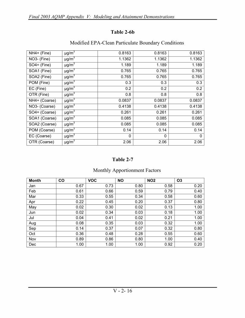
Final 2003 AQMP Appendix V: Modeling and Attainment Demonstrations
V - 2- 16
Table 2-6b
Modified EPA-Clean Particulate Boundary Conditions
NH4+ (Fine) µg/m3 0.8163 0.8163 0.8163NO3- (Fine) µg/m3 1.1362 1.1362 1.1362SO4= (Fine) µg/m3 1.189 1.189 1.189SOA1 (Fine) µg/m3 0.765 0.765 0.765SOA2 (Fine) µg/m3 0.765 0.765 0.765POM (Fine) µg/m3 0.3 0.3 0.3EC (Fine) µg/m3 0.2 0.2 0.2OTR (Fine) µg/m3 0.8 0.8 0.8NH4+ (Coarse) µg/m3 0.0837 0.0837 0.0837NO3- (Coarse) µg/m3 0.4138 0.4138 0.4138SO4= (Coarse) µg/m3 0.261 0.261 0.261SOA1 (Coarse) µg/m3 0.085 0.085 0.085SOA2 (Coarse) µg/m3 0.085 0.085 0.085POM (Coarse) µg/m3 0.14 0.14 0.14EC (Coarse) µg/m3 0 0 0OTR (Coarse) µg/m3 2.06 2.06 2.06
Table 2-7
Monthly Apportionment Factors
Month CO VOC NO NO2 O3 Jan 0.67 0.73 0.80 0.58 0.20Feb 0.61 0.66 0.59 0.79 0.40Mar 0.33 0.55 0.34 0.58 0.60Apr 0.22 0.45 0.20 0.37 0.80May 0.02 0.30 0.02 0.13 1.00Jun 0.02 0.34 0.03 0.18 1.00Jul 0.04 0.41 0.02 0.21 1.00Aug 0.08 0.35 0.03 0.32 1.00Sep 0.14 0.37 0.07 0.32 0.80Oct 0.36 0.48 0.28 0.55 0.60Nov 0.89 0.86 0.80 1.00 0.40Dec 1.00 1.00 1.00 0.92 0.20

Chapter 2 PM10 Attainment and Visibility
V - 2- 17
Three-Dimensional Temperature and Humidity Fields UAMAERO-LT required gridded three-dimensional temperature and humidity fields as input for the particulate and gaseous chemistry. Three-dimensional temperature and humidity fields were developed from the available surface and upper air data using Poisson objective analysis techniques. Data from 16 District air monitoring stations and FAA airport observations provided characterization of the daily surface temperature and humidity fields. An additional eight pseudo-stations were created from this data base to characterize offshore temperature and humidity profiles and to represent desert and mountain boundary conditions. The hourly surface fields were subjected to a 5-point filter to smooth gridded temperature variations.
Hourly temperature and humidity profiles through 2000 m aloft were interpolated from the morning (0400 PST) and afternoon (1600) coastal sounding profile taken at Miramar Naval Air Station (NKX). The gridded hourly surface fields were merged with the hourly upper level profiles and were vertically averaged by grid to match the five vertical layers determined by the mixing height specification for the UAMAERO-LT simulations.
Use of the 3-dimensional temperature field for the UAMAERO-LT simulations negated the need to specify temperature lapse rates above and below the mixing height as required by the U.S. EPA version of the UAM during modeling applications.
Mixing Heights Mixing was calculated using a Holzworth (1964) approach, which estimates the extent of buoyant vertical lifting of an air parcel based on the surface temperature of the air parcel and that of the environment lapse rate measured by the morning and afternoon soundings at NKX. The basic process is summarized in Technical Report V-B of the 1994 AQMP.
The major modification to the mixing calculation was to superimpose a set of criteria for adjusting daily minimum, and daily minimum-maximum mixing heights. The criteria are summarized in Table 2-8. The monthly values set for the minimum-maximum mixing height in the coastal and mid-basin areas were based on the calculated 1995 daily maximum mixing at Central Los Angeles. The minimum-maximum mixing heights ranged from 750 m in the mid-summer months to 850 m in winter and spring. This modification was made to adjust mixing in the low elevation stations when cool surface temperatures observed in the marine modified air restricted the buoyant mixing height calculation, yet a defined marine layer was present.

Final 2003 AQMP Appendix V: Modeling and Attainment Demonstrations
V - 2- 18
Table 2-8
Mixing Height Adjustment Criteria
Minimum Mixing Heights
Station/Zone Station Height (Ft) Above Sea Level
Mixing Height (m)
Coastal 0-100 150
Mid-Basin 100-500 100
Inland-Basin 600-1700 50
Mountains > 1700 50
Deserts Variable 50
Minimum Assigned Height for Maximum Mixing
Station/Zone Station Height (Ft) Above Sea Level
Mixing Height (m)
Coastal 0-100 Monthly Profile
Mid-Basin 100-500 Monthly Profile
Inland-Basin 600-1700 Calculated
Mountains > 1700 Calculated
Deserts Variable Calculated
The maximum daily mixing heights were capped at 2000 m. On "rain-days" when 0.01 inches of precipitation was measured in the Basin the mixing was raised to 2000 m for all 24-hours. The final gridded mixing height fields were subjected to smoothing with time and space.
Wind Fields The hourly wind fields used by the UAMAERO-LT were generated using the Hybrid Diagnostic Wind Model (HDWM) developed by Douglas and Kessler (1988). The HDWM approach, which incorporates a diagnostic wind algorithm with objective analysis, is described in Technical Report V-B of the 1994 AQMP.
For wind field generation, the diagnostic model utilized wind barriers to assist in characterizing flow through the complex terrain. Winds were generated for a 5 km square grid with 19 vertical layers. Three-dimensional winds were generated using the diagnostic assumption coupled with objective analysis using all available upper air winds and hourly averaged wind data at the surface.

Chapter 2 PM10 Attainment and Visibility
V - 2- 19
The District surface wind observations, routinely monitored at 33 locations, were used to characterize hourly wind fields in the mixed layer for the annual UAMAERO-LT modeling application. Winds aloft (1500m) were characterized by synoptic winds extrapolated from the daily 0400 and 1600 PST 850 millibar surface analyses. Key upper air locations included Vandenberg AFB, San Diego, Las Vegas and a mid-basin location, approximately Ontario. These upper air wind data were merged with hourly radar wind profiles measured at LAX.
In the preparation of the HDWM input files for the UAMAERO-LT annual model application, the 1500 m synoptic winds were assigned to characterize all layers above 1000 m. Winds between the surface and the 1000 m level were interpolated from the surface observations using a “power law” profile.
UAM layer-averaged winds were created from the HDWM wind modeling techniques using a layer matching scheme (UAMWND) developed by Douglas et al. (1990), which weights surface layer wind influence to layers aloft on the basis of stability. For the UAMAERO-LT annual application, winds were averaged into a 5-layer format (two below the mixing height and three above). The 3-dimensional winds were converted to a 5-layer format using the UAM layer-matching scheme and the gridded matrix of hourly mixing heights.
Additional post-processing techniques were selectively applied to the UAM wind fields generated using one or more of the above methodologies. These included the use of a 5-point filter to smooth a UAM wind field to dampen horizontal shear, and use of a filtering technique [which follows a profile suggested by O’Brien (1970)] to adjust UAM vertical velocities and dampen mass flow through the top of the modeling domain.
Rain Days
Precipitation summaries were reviewed to determine the dates on which measurable rainfall (0.01 inches or more in the South Coast Drainage Division) fell in the Basin during 1995. A total of 56 days met this criterion in the Basin for 1995. Table 2-9 lists the dates meeting this criterion. This data was used by the preprocessor to seasonally adjust entrained and wind blown dust emissions by a rain-factor. The rain-factor adjustment was taken from EPA AP-42 (Fifth Edition, Volume 1) 13.2.1--Paved Roads. The seasonal rain-factor adjustment was made on a quarterly basis. The rain factor adjustment was applied to all fugitive dust emissions categories. In addition, the photolysis rate used by UAMAERO-LT was reduced by 40 percent on rain days to account for insolation reduction due to cloud cover.

Final 2003 AQMP Appendix V: Modeling and Attainment Demonstrations
V - 2- 20
9-Cell Averaging
A nearest cell average of predicted concentrations is typically used when comparing gridded concentrations to station measurements, because of possible spatial misalignments of the predicted concentration fields. The UAMAERO-LT modeling results are presented based on a nearest nine-grid-cell average basis. Performance evaluations at each station are based on this average concentration.
Table 2-9
1995 Rain Days in the Basin: Days Recording Measurable Precipitation of at least 0.01 Inches of Rain
Month Dates January 3, 4, 5, 7, 8, 9, 10, 11, 12, 13, 15, 16, 17, 21, 23, 24, 25, 26 February 8, 9,13, 14,15 March 2, 3, 4, 5, 6, 7, 10, 11, 12, 21, 22, 23, 24 April 16, 17, 18 May 14,15, 22, 23, 24 June 1, 15, 16, 17 July 16 September 1, 2 October 31 November 1 December 13, 14, 16, 23, 24
Linear Rollback For 24-Hour Average Maximum Concentrations
Linear rollback on particulate component species is used to assess future year 24-hour maximum PM10 concentrations at the five PTEP monitoring sites. Observed 24-hour average maximum PM10 for 1995 are used to anchor the rollback calculation for future year impacts. For Rubidoux, the 1995 annual second maximum PM10 concentration (206 µg/m3) is used for the analysis since the peak 24-hour average (219 µg/m3) occurred during “Santa Ana” high winds. This day, (April 9, 1995), has not been tagged as a natural event in the AIRS data set since the policy did not take effect until 1997. (The primary portion of the PM10 mass sampled at Rubidoux on April 9, 1995 was 192 µg/m3, or 88 percent of the total). It is useful to note that the 24-hour PM10 standard has been exceeded on only 16 days since 1995 with 10 of those days having high winds. In addition, since 1997, only high wind conditions have caused the 24-hour standard to be exceeded.

Chapter 2 PM10 Attainment and Visibility
V - 2- 21
The methodology used to conduct the linear rollback calculations is described at length in Appendix V of the 1997 AQMP. Briefly, the linear rollback approach used to predict component particulate concentrations for 2006 and 2010 assumes that the ambient concentrations above background levels are directly proportional to the different emissions species in the inventory. In mathematical terms, the rollback relationship can be written as follows:
Cp = [(Cb - k) • Qp/Qb] + k
where Cp and Cb are the future year and baseline PM10 component concentrations (e.g., sulfate), respectively; Qp and Qb are the future year and baseline PM10 component emission rates (e.g., sulfur dioxide), respectively; and k denotes the global background PM10 component concentration (e.g., sulfate). For most PM10 components it is assumed that global background concentrations are negligible; therefore the above equation simplifies to
Cp = Cb • Qp/Qb.
The rollback calculation is conducted on each individual species. The net rollback is the summation of the individual predicted changes.
EMISSIONS INVENTORY
The UAMAERO-LT model requires several emissions, aerometric, and meteorological data inputs. These input data are similar to those needed for the UAM ozone simulations. The ozone simulation requires day-specific emissions inventories, which account for variations in observed diurnal traffic patterns and large source emissions profiles. UAMAERO-LT model is based on the annual average inventory, with adjustments made for weekly and monthly variations. A brief characterization of the annual day emissions used for the UAMAERO-LT modeling analysis follows. An extensive discussion of the overall emissions inventory is summarized in the 2003 AQMP Appendix III.
The 1997 emissions inventory was backcasted to 1995 to establish an inventory for the base year UAMAERO-LT modeling application. The 1995 emissions inventory is summarized in Table 2-10, along with projected baseline inventories for the years 2006, and 2010. Also presented in Table 2-10 are the inventories reflecting implementation of the control strategy for 2006, and two options for control in 2010. Annual average day emissions are presented for six categories: volatile organic compounds (VOC), oxides of nitrogen (NOx), oxides of sulfur (SOx), diesel particulates (Diesel), geological particulates (Geologic), and total primary PM10 (Primary).

Final 2003 AQMP Appendix V: Modeling and Attainment Demonstrations
V - 2- 22
A seasonally based biogenic emissions inventory (not listed in Table 2-10) was developed by the California ARB. The inventory was temperature corrected for both winter and summer profiles. The summer biogenic inventory was used from April through September. The winter inventory was used for the remaining months.
Where applicable, point, area and off-road mobile sources were adjusted to a day-of-week through-put profile consisting of a Monday-Friday, Saturday and Sunday schedule. On-road mobile sources were also adjusted by the same day-of-week schedule and overlaid with average diurnal profiles that represent weekday and weekend defined traffic patterns. The on-road mobile source emission data incorporate month specific ambient temperature and humidity input.
Emissions Uncertainties
Uncertainties can be estimated for all sources of emission: point, mobile, and area. With regard to PM10 prediction, quantification, spatial allocation and apportionment of dust sources is magnified. The following sections address uncertainties selected estimated of PM10 dust emissions.
Paved Road Dust
Paved road dust accounted for the largest percentage of the primary emissions category. In addition, the paved road dust emissions are a function of VMT. In the 1997 and 2003 AQMP, paved road dust emissions used in the UAM/LC runs were adjusted to reflect a cap on emissions growth for high VMT road types in future years. Base year emissions were not capped at a given VMT level. The future year adjustment assumed that the silt loading would be depleted by the entrainment from the traffic volume. Increasing the traffic volume beyond a set point would not increase dust entrainment because the silt would be essentially depleted. Analysis of model results indicate the paved road dust may be overestimated by a factor of two in Los Angeles and Orange Counties where the traffic volume is greatest. The overestimation is lower in Riverside and San Bernardino Counties. Overestimation is also evident in grids having multiple freeways or large thoroughfares. This indicates that emissions may cease to be a function of VMT at lower VMT levels than used in the base year estimations.

Chapter 2 PM10 Attainment and Visibility
V - 2- 23
TABLE 2-10 UAMAERO-LT Annual Average Day Emissions Inventory (Tons/Day)
Year VOC NOx SOx Diesel Geol Primary
(a) Baseline
1995 1306.7 1440.1 107.9 23.8 236.8 313.5
2006 689.2 942.7 59.5 19.9 203.5 291.9
2010 614.7 771.0 60.1 17.5 209.9 298.3
(b) Controlled
2006 673.8 935.4 57.3 19.9 203.5 290.8
2010 Option–1 294.9 543.0 58.9 12.1 209.9 290.6
2010 Option-2 298.4 611.0 58.9 13.8 209.9 292.5
A modeling sensitivity run was conducted to assess the paved road dust contribution to predicted PM10 by eliminating paved road dust emissions and comparing predicted annual concentrations to those for a parallel run having paved road dust. Paved road dust emissions are approximately 50 percent of all PM10 emissions in the Basin. In Los Angeles County, the average paved road dust contribution to PM10 was 9.9 µg/m3 or 55 percent of the average predicted concentration other category. The average value for Orange county was 9.4 µg/m3 or 58 percent of the predicted other category concentration. In contrast, the paved road dust contributions to Riverside and San Bernardino Counties were 6.4 and 8.3 µg/m3 or, 33 and 34 percent of the predicted other category concentration, respectively. The 1995 measured annual average concentrations for the other category from Central Los Angeles and Anaheim were 13.0 µg/m3 and 13. µg/m3, respectively. In the sensitivity analysis, the predicted paved road dust contribution to the others category for those sites was 12.5 µg/m3 for Anaheim and 12.6 µg/m3 at Central Los Angeles. The regional background concentration for the others category is approximately 8 µg/m3, (see San Nicholas Island in Figure 2.2). The results of the sensitivity analysis indicate that the relative percentage contribution from paved road dust to the predicted primary "others" category is significantly higher than the 50 percent weighting the paved road dust has to the total inventory and may be more than doubled the actual loading.
Unpaved Road Dust
Uncertainties exist in determining both total unpaved road dust emissions and their location (c.f. CARB’s emission methodology, Section 7.10, “Unpaved Road Dust”).

Final 2003 AQMP Appendix V: Modeling and Attainment Demonstrations
V - 2- 24
Regional estimates are based on relatively broad assumptions of miles of unpaved road miles (e.g. 1989 Caltrans data) and trip activity (e.g., 10 ADT). Such estimates likely overestimate unpaved road emissions in the western Basin (e.g., more development and paving projects in recent years) and underestimate emissions in the eastern Basin (e.g. fewer 1989 Caltrans-maintained roads in previously lower population areas). In addition, the spatial distribution of unpaved roads is problematic. Common surrogates, such as population, may not be appropriate in certain subregions. As noted by CARB, better mileage information could possibly be obtained from GIS-based maps, especially for subregions. Coupled with traffic counts on key roads, a better subregional inventory could be developed, if necessary.
Fugitive Wind Blown Dust
Fugitive wind blown dust emissions were another source of emissions uncertainty. Uncertainties occur in the emission estimation methodology, spatial allocation and in the inability of the annual average day to accurately incorporate the impacts of high-wind events. The original fugitive dust emissions are defined as annual average day county total. The emissions were allocated by pastureland acreage based on a GIS apportionment of dust to areas of each county designated as pastureland in the Basin. This allocation may have reduced the windblown dust contribution to the Rubidoux area shifting a majority of the Riverside County dust towards the Perris and Hemet areas. For the Mojave Desert Air Basin portion of San Bernardino County, the wind blown dust allocation forced a significant amount of dust emissions into a limited number of grid cells. Similarly, there was a significant amount of uncertainty associated with gridded allocation of windblown dust from unpaved roads. A similar cluster of "hot" grid-cells appears in the Mojave Desert, north of the Cajon Pass.
The impact of "Santa Ana" high wind events on the fugitive windblown dust emissions cannot be well simulated through the annual modeling. Wind trajectories are highly localized and may impact one area more than another. A classic case occurred on April 9, 1995 at Rubidoux where 24-hour average concentrations measured 219 µg/m3 under strong Santa Ana winds. Sulfate, nitrate and chloride accounted for 11 percent of the mass while the majority of the remaining mass (195 µg/m3) fell into the primary (others) category. The total mass observed on this day accounts for 3.6 percent of the annual average, mostly due to high winds. On the same day, the neighboring sites of Norco and Ontario measured 24-hour averages of PM10 of 64 and 66 µg/m3 respectively. These values are roughly one third of the Rubidoux concentration. The capricious nature of wind blown dust, demonstrated through the PM10 concentrations measured on April, 9, 1995, is summarized in Table 2-11.
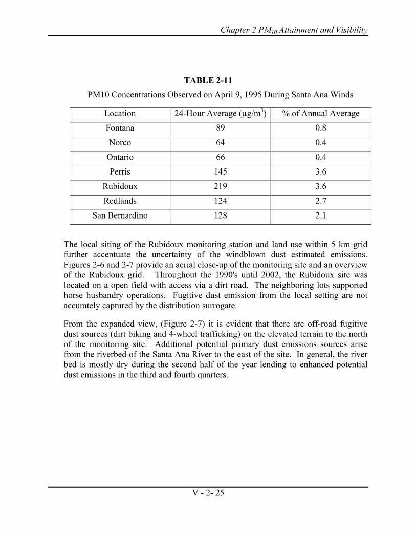
Chapter 2 PM10 Attainment and Visibility
V - 2- 25
TABLE 2-11 PM10 Concentrations Observed on April 9, 1995 During Santa Ana Winds
Location 24-Hour Average (µg/m3) % of Annual Average
Fontana 89 0.8
Norco 64 0.4
Ontario 66 0.4
Perris 145 3.6
Rubidoux 219 3.6
Redlands 124 2.7
San Bernardino 128 2.1
The local siting of the Rubidoux monitoring station and land use within 5 km grid further accentuate the uncertainty of the windblown dust estimated emissions. Figures 2-6 and 2-7 provide an aerial close-up of the monitoring site and an overview of the Rubidoux grid. Throughout the 1990's until 2002, the Rubidoux site was located on a open field with access via a dirt road. The neighboring lots supported horse husbandry operations. Fugitive dust emission from the local setting are not accurately captured by the distribution surrogate.
From the expanded view, (Figure 2-7) it is evident that there are off-road fugitive dust sources (dirt biking and 4-wheel trafficking) on the elevated terrain to the north of the monitoring site. Additional potential primary dust emissions sources arise from the riverbed of the Santa Ana River to the east of the site. In general, the river bed is mostly dry during the second half of the year lending to enhanced potential dust emissions in the third and fourth quarters.

Final 2003 AQMP Appendix V: Modeling and Attainment Demonstrations
V - 2- 26
Figure 2-6 Rubidoux Air Monitoring Station and Immediate Surrounding Area
Construction Dust
The location of PM10 emissions from construction activities presents a third area of uncertainty to the analysis. The surrogate used to allocate 1995 Basin construction dust emissions was the number of building permits issued by individual cities, within each of the four counties. The building permit survey was based on construction year 2000. The assumption was made that the cities and relative numbers of permits issued were consistent between 1995 and 2000. The estimated countywide emissions were apportioned by city and the dust emissions were uniformly distributed within the city's geographical boundaries. While this methodology brought the construction dust emissions closer to the actual activities, the spatial resolution within each city was still coarse whereby neighboring grids would be underestimated and others overestimated. In addition, the assumption that 2000 directly represented 1995 introduced additional uncertainty.
Rubidoux Monitoring Station

Chapter 2 PM10 Attainment and Visibility
V - 2- 27
Figure 2-7 Rubidoux Air Monitoring Station and Immediate Surrounding Area
The uncertainty of the construction dust emissions is clearly evident at the Fontana air monitoring site in 1995. In October 1995, construction began on the California Speedway. The construction site was approximately one square mile in area and was located one kilometer upwind of the Fontana monitoring site. Figure 2-8 presents the locations of the California Speedway and the Fontana monitoring site. Based on the project's environmental impact report, after mitigation actions, dust emissions from the project were estimated at 1,450 kg per day. Using EPA's ISCST point source dispersion model and an annual meteorological data set for Fontana, a potential quarterly impact from the construction grading operations was estimated to be 5.2 µg/m3, or 1.3 µg/m3 to the annual average. These emissions and projected impacts were not captured by the spatial and temporal allocation of the construction emissions. As a consequence, it is expected that the primary prediction would be under represented by the regional modeling analysis for the base year.
Rubidoux Monitoring Station

Final 2003 AQMP Appendix V: Modeling and Attainment Demonstrations
V - 2- 28
Additional uncertainty is introduced for the future baseline emissions where projections of population growth, employment and population density, were used to apportion construction dust.
Figure 2-8
Fontana Air Monitoring Station and Immediate Surrounding Area
BASE-YEAR SIMULATIONS
UAMAERO-LT was run for the 1995 base simulation using the annual average day emissions presented in the previous emission inventory discussion and the meteorological and air quality data inputs outlined in the preceding section. EPA guidance focuses model performance to the ability to predict the PM10 component species and the total mass. Three elements are presented in this section to address model performance guidance and quantify the base-year performance: (1) the PM10 component species performance evaluation for the PTEP sites, (2) the annual average
Fontana Monitoring Station

Chapter 2 PM10 Attainment and Visibility
V - 2- 29
performance evaluation for total mass at the SSI PM10 sites, and (3) the analysis of the 1995 gridded simulation.
PM10 Component Species Performance Evaluation for the PTEP Sites
The UAMAERO-LT 1995 base-year PM10 annual average predicted PM10 and observations for the six component species at the five Basin PTEP sites are presented in Table 2-12. In general, ammonium is well predicted at all sites. Nitrate tends to be over predicted at most sites with the exception of Rubidoux. In contrast, the simulation tends to under predict sulfate and elemental carbon at all sites but the concentration differential is typically 2 µg/m3 or less. Los Angeles and Anaheim clearly exhibit over prediction of mass in the primary category, most likely due to uncertainties in the paved road dust emission inventory. Fontana and Rubidoux are under predicted in the primary category due to uncertainties in the allocation of the fugitive dust, farming operation dust and construction dust categories.
TABLE 2-12 UAMAERO-LT 1995 Base Year Model Predictions (µg/m3)
Compare to Annual Average Observations (µg/m3)
Anaheim Diamond Bar Fontana Los Angeles Rubidoux Component Predicted Observed Predicted Observed Predicted Observed Predicted Observed Predicted Observed
Ammonium 4.5 4.0 4.8 4.6 5.7 4.6 4.0 4.0 6.2 5.9
Nitrate 13.6 10.4 15.2 11.8 17.2 13.4 11.8 9.9 18.9 17.5
Sulfate 2.8 4.8 2.6 4.3 3.3 3.6 2.7 4.3 2.8 4.0
Organic Carbon 6.9 7.4 6.6 8.6 6.4 10.4 7.2 8.5 7.0 10.5
Elemental Carbon
2.2 2.9 1.9 3.5 2.2 3.7 2.3 3.6 2.6 3.1
Primary 19.5 13.8 16.7 13.1 20.0 25.2 20.8 13.0 19.3 27.8
Total Mass 49.5 43.5 47.8 46.0 54.8 61.0 48.8 42.8 56.8 69.0

Final 2003 AQMP Appendix V: Modeling and Attainment Demonstrations
V - 2- 30
UAMAERO-LT Component Species Model Performance Evaluation
Draft Working Paper #M-2, “PM10 Modeling Protocol for the 1997 Air Quality Management Plan Revision” (Zhang et.al.,) outlines a series of performance goals that were established to estimate the ability of the UAMAERO-LT to recreate annual PM10. The performance goals express average prediction error over the five sites for each of the component species. Table 2-13 summarizes the UAMAERO-LT annual performance goals.
The performance statistics for the UAMAERO-LT 1995 base case annual simulation are presented in Table 2-14. Percent prediction error is presented for each component species at the five Basin PTEP sites.
TABLE 2-13 UAMAERO-LT Performance Goals
Species Goal (%) Comparison Basis
Sulfate ± 30 Annual Average
Nitrate ± 30 Annual Average
Ammonium ± 30 Annual Average
Primary ± 30 Annual Average
Overall, the performance of the UAMAERO-LT averaged over the five stations is within or near the goals defined in Table 2-13. Predictions of ammonium and nitrate were within the 30 percent error performance criteria at all stations for the base case application. The five station average error for ammonium, nitrate and organic carbon were 9.7, 23.7, and 23.4 percent, respectively. Percentage errors for sulfate prediction at Anaheim, Diamond Bar, Los Angeles and Rubidoux exceeded the 30 percent threshold. When taken collectively, the five station average is calculated at 33.9 percent. This statistic is somewhat misleading however since the annual average concentrations of sulfates measured at each of these stations were less than 5.0 µg/m3, and bias in the prediction performance was typically less than 2.0 µg/m3. A similar observation can be made for elemental carbon.
Percent errors for primary particulates at Anaheim, and Los Angeles reflect uncertainties in the gridded primary particulate emissions inventory for the more urbanized western half of the Basin. Percentage errors in prediction performance at

Chapter 2 PM10 Attainment and Visibility
V - 2- 31
Diamond Bar, Fontana and Rubidoux, stations located in the eastern half of the Basin that experience greater, and more frequent, primary emissions impacts, meet or are close to the goals set for model performance.
Figures 2-9 through 2-13 present scatter plots of predicted and observed concentrations of the six components. In the figures, the 30 percent error bars are drawn on each side of the unity line. Only a few predictions in the nitrate category are beyond the 30 percent error bounds with most of the predictions for the other components falling within bounds. Figures 2-14 through 2-18 depict the time series of predicted 24-hour average total and observations for each of the six components at each PTEP site. What is evident from the scatter plots and the time series analyses is that the model responds to changes in daily meteorology and captures the seasonal variation of particulate formation. The simulation is poorest in the first quarter during rapid transitions between rain events. Otherwise, component concentrations tend to follow observations with the peak concentrations (predicted and observed) occurring the fall.
TABLE 2-14 UAMAERO-LT Performance Statistics (annual percent absolute error)
Species Location Ammonium Nitrate Sulfate Organic
carbon Elemental
carbon Primary
Anaheim 12.5 29.5 42.9 6.7 24.1 40.3 Diamond Bar 4.3 28.8 39.5 23.3 45.7 27.4 Fontana 23.9 28.3 8.3 38.5 40.5 20.9 Los Angeles 2.6 21.6 35.7 15.3 37.8 63.8 Rubidoux 5.1 10.3 30.0 33.3 18.8 30.8
Average 9.7 23.7 31.3 23.4 33.4 36.6
Annual Average SSI Mass Performance Evaluation
As part of the weight of evidence discussion, the base-year performance evaluation is presented for the UAMAERO-LT simulation comparing the predicted and observed annual average mass at the District's SSI monitoring network and at SSI sites in neighboring air basins included in the modeling domain. The goal of this analysis is to demonstrate that the model is capable of simulating PM10 not only at the key sites but across the modeling domain. Table 2-15 summarizes the UAMAERO-LT performance for annual average mass at the SSI sites. Figures 2-19 through 2-21

Final 2003 AQMP Appendix V: Modeling and Attainment Demonstrations
V - 2- 32
provide the time series of the 24-hour averaged predicted PM10 and observed mass at the SSI sites.
With the exceptions of Banning and Crestline, the simulated annual average PM10 concentrations fall with the 30 percent goal at all Basin SSI sites. It is important to note that the station predictions represent a nine-grid cell average. In general, the east Basin sites tend to be under predicted with the notable exceptions of Ontario and Pomona/Diamond Bar. The remaining Los Angeles County sites are mixed with a slight bias towards over prediction. The two Orange County sites are over predicted by an average of 24 percent.
Table 2-15
UAMAERO-LT Predicted and SSI Observed 1995 Base-Year Annual Average PM10 Concentrations
Location Predicted Annual Average Concentration (µg/m3)
Observed Annual Average Concentration (µg/m3)
Percentage Prediction Error
Central LA 48.6 42.8 13.6 Hawthorne 34.0 36.2 -6.1 N. Long Beach 46.3 38.7 19.6 Burbank 45.0 42.2 6.6 Azusa 44.4 49.1 -9.6 Pomona/Diamond Bar 47.2 46.0 2.6 Santa Clarita 41.8 37.0 13.0 Anaheim 49.5 43.5 13.8 El Toro 46.2 37.6 22.9 Norco 57.3 54.2 5.7 Rubidoux 56.5 69.0 -18.1 Perris 45.4 46.7 -2.8 Banning 21.3 30.1 -29.2 Ontario 60.7 54.0 12.4 Fontana 54.8 61.0 -10.2 San Bernardino 52.9 57.3 -7.7 Redlands 40.5 48.4 -16.3 Crestline 43.5 20.4 113.2 Thousand Oaks 36.7 27.0 35.9 Simi Valley 39.3 28.0 40.4 Piru 26.9 27.0 -0.4 Lancaster 17.8 25.6 -30.4 Hesperia 60.4 14.0 331.4 Victorville 57.7 12.0 380.8

Chapter 2 PM10 Attainment and Visibility
V - 2- 33
FIGURE 2-9
Predicted and Observed 24-Hour Average PM10 Anaheim

Final 2003 AQMP Appendix V: Modeling and Attainment Demonstrations
V - 2- 34
Figure 2-10
Predicted and Observed 24-Hour Average PM10 Central Los Angeles

Chapter 2 PM10 Attainment and Visibility
V - 2- 35
Figure 2-11
Predicted and Observed 24-Hour Average PM10 Diamond Bar

Final 2003 AQMP Appendix V: Modeling and Attainment Demonstrations
V - 2- 36
Figure 2-12
Predicted and Observed 24-Hour Average PM10 Fontana

Chapter 2 PM10 Attainment and Visibility
V - 2- 37
Figure 2-13
Predicted and Observed 24-Hour Average PM10 Rubidoux

Final 2003 AQMP Appendix V: Modeling and Attainment Demonstrations
V - 2- 38
Figure 2-14
Time Series of Predicted and Observed 24-Hour Average PM10 Anaheim

Chapter 2 PM10 Attainment and Visibility
V - 2- 39
Figure 2-15
Time Series of Predicted and Observed 24-Hour Average PM10 Central L.A.

Final 2003 AQMP Appendix V: Modeling and Attainment Demonstrations
V - 2- 40
Figure 2-16
Time Series of Predicted and Observed 24-Hour Average PM10 Diamond Bar

Chapter 2 PM10 Attainment and Visibility
V - 2- 41
Figure 2-17
Time Series of Predicted and Observed 24-Hour Average PM10 Fontana

Final 2003 AQMP Appendix V: Modeling and Attainment Demonstrations
V - 2- 42
Figure 2-18
Time Series of Predicted and Observed 24-Hour Average PM10 Rubidoux

Chapter 2 PM10 Attainment and Visibility
V - 2- 43
Figure 2-19
Time Series of Predicted and Observed 24-Hour Average PM10 at SSI Sites

Final 2003 AQMP Appendix V: Modeling and Attainment Demonstrations
V - 2- 44
Figure 2-20
Time Series of Predicted and Observed 24-Hour Average PM10 at SSI Sites

Chapter 2 PM10 Attainment and Visibility
V - 2- 45
Figure 2-21
Time Series of Predicted and Observed 24-Hour Average PM10 At SSI Sites

Final 2003 AQMP Appendix V: Modeling and Attainment Demonstrations
V - 2- 46
1995 UAMAERO-LT Grid-Cell Performance Evaluation
Figure 2-22 presents the grid cell predicted annual average PM10 predictions for the 1995 base-year. As demonstrated from the predicted and observed SSI station analysis, grid cell based simulation demonstrates a west to east gradation in predicted PM10 with Basin peak predicted annual average concentrations coinciding with the areas defined by the SSI data depicted in Figure 2-4.
Noted in the analysis are several grid cells exhibiting high "hot-spot" values of PM10 in areas where predicted particulate levels are estimated to be above the regional profile. The primary areas of over prediction occur in the San Fernando Valley (an area dominated by paved road and construction dust emissions) and in the Basin portions of San Bernardino and Riverside Counties (where wind blown fugitive dust is added to construction and paved road dust impacts).
Additional "hot-spot" grid cells are identified in the Corona, Chino, Ontario and Fontana-Rialto areas of Riverside and the Basin portion of San Bernardino Counties. The impacts of the "hot spot" grid cells on the future year PM10 predictions and the uncertainties of the primary emissions in those grid cells are addressed in a following section.
Figure 2-22
1995 UAMAERO-LT Grid-Cell Performance Evaluation (Grid Cell Predicted Concentrations in µg/m3 )

Chapter 2 PM10 Attainment and Visibility
V - 2- 47
PM2.5 Component Species Performance Evaluation for the PTEP Sites
The UAMAERO-LT 1995 base-year annual average predicted PM2.5 and observations for the six component species at the five Basin PTEP sites are presented in Table 2-16. In general, ammonium is well predicted at most sites with Fontana being under predicted. Nitrate tends to be over predicted at most sites with the exception of Rubidoux. In contrast, the simulation tends to under predict sulfate, organic carbon and elemental carbon at all sites but the concentration differential is typically 2 µg/m3 or less. PM2.5 mass in the primary category is clearly over predicted at all sites. The over prediction in the primary category tends to offset the under prediction in sulfate, organic carbon and elemental carbon. The net result is for a close prediction of total PM2.5 mass at all site except Anaheim .
TABLE 2-16 UAMAERO-LT 1995 Base Year PM2.5 Model Predictions (µg/m3)
Compare to Annual Average Observations (µg/m3)
Anaheim Diamond Bar Fontana Los Angeles Rubidoux Component
Predicted Observed Predicted Observed Predicted Observed Predicted Observed Predicted Observed
Ammonium
4.2 4.3 4.2 4.6 5.1 4.7 3.3 3.9 5.2 6.1
Nitrate
10.6 8.2 10.9 9.3 12.5 10.8 8.0 7.5 13.3 14.7
Sulfate
2.3 4.2 2.1 4.0 2.7 3.8 2.1 3.7 2.1 3.2
Organic Carbon
5.1 6.2 4.4 6.4 4.7 7.2 4.9 6.5 4.9 6.4
Elemental Carbon
2.0 2.7 1.7 3.3 2.0 3.3 1.9 3.4 1.9 2.8
Primary
5.8 0.7 5.1 0.1 6.5 2.0 5.8 0.1 5.5 2.6
Total Mass
30.0 26.3 28.4 27.7 33.4 31.8 26.0 25.1 33.0 35.8
FUTURE AIR QUALITY
Future-year PM10 air quality is projected using the procedures and assumptions previously described. Emissions for the 2006 and 2010 baseline and controlled scenarios are listed in Table 2- 10.

Final 2003 AQMP Appendix V: Modeling and Attainment Demonstrations
V - 2- 48
The federal annual average PM10 standard is 50.4 µg/m3, and it is calculated as an annual arithmetic mean; the federal 24-hour average PM10 standard is 150 µg/m3.
The state PM10 air quality standards are stricter than the federal PM10 standards. The state annual PM10 standard is 20 µg/m3 (also based on an annual arithematic mean), and the state 24-hour average PM10 standard is 50 µg/m3. There is no requirement to comply with the state PM10 standards by a specified date. However, future-year annual average PM10 concentrations show the progress toward the attainment of the state PM10 air quality standards.
The UAMAERO-LT simulation with emission controls shows that the Basin will attain the annual federal PM10 standard by the year 2006. In addition, linear rollback with emission controls show that the Basin will attain the 24-hour average federal PM10 standard by the year 2006. However, the analysis indicates that the more restrictive state annual and 24-hour average PM10 standards will not be met in all areas of the Basin by 2010.
The future year PM10 discussion follows the order of the previous analysis on base year model performance evaluation. Future year PM10 is presented for: (1) the PM10 component species at the PTEP sites, (2) the annual average for total mass at the SSI PM10 sites, and (3) the 2006 gridded simulation and weight of evidence "hot-spot" grid analysis.
For the purpose of the Basin attainment demonstration, analyses of predicted PM10 outside the District jurisdiction are not presented in this draft analysis.
PM10 Control Strategy
The PM10 control strategy is component of the overall control strategy presented in Chapter 4 of the 2003 AQMP. Aside from directly emitted PM10, emissions reductions for VOC, NOx and ammonia are required to bring the Basin into compliance of the annual average and 24-hour average standards by the year 2006 and maintain those standards in 2010. The majority of the VOC and NOx emissions reductions projected by 2006 come from implementation of measures in the mobile, point and area sources categories and fleet turnover. The 1997 AQMP introduced several control measures to reduce directly emitted PM10, and address VOC and ammonia emissions from agricultural operations that will impact 2006 emissions. The 2003 AQMP Short-Term strategy continues the implementations of several measures that were introduced in the 1997 AQMP. These measures address PM10 VOC and ammonia emissions from livestock waste (WST-01), composting (WST-02) restaurant operations (PRC-03), and emissions reductions from petroleum fluid catalytic cracking units (CMB-09). Newly proposed control measures include further reduction to fugitive dust sources (BCM-07), further emission reduction from aggregate cement plant manufacturing operations (BCM-08), emissions reductions
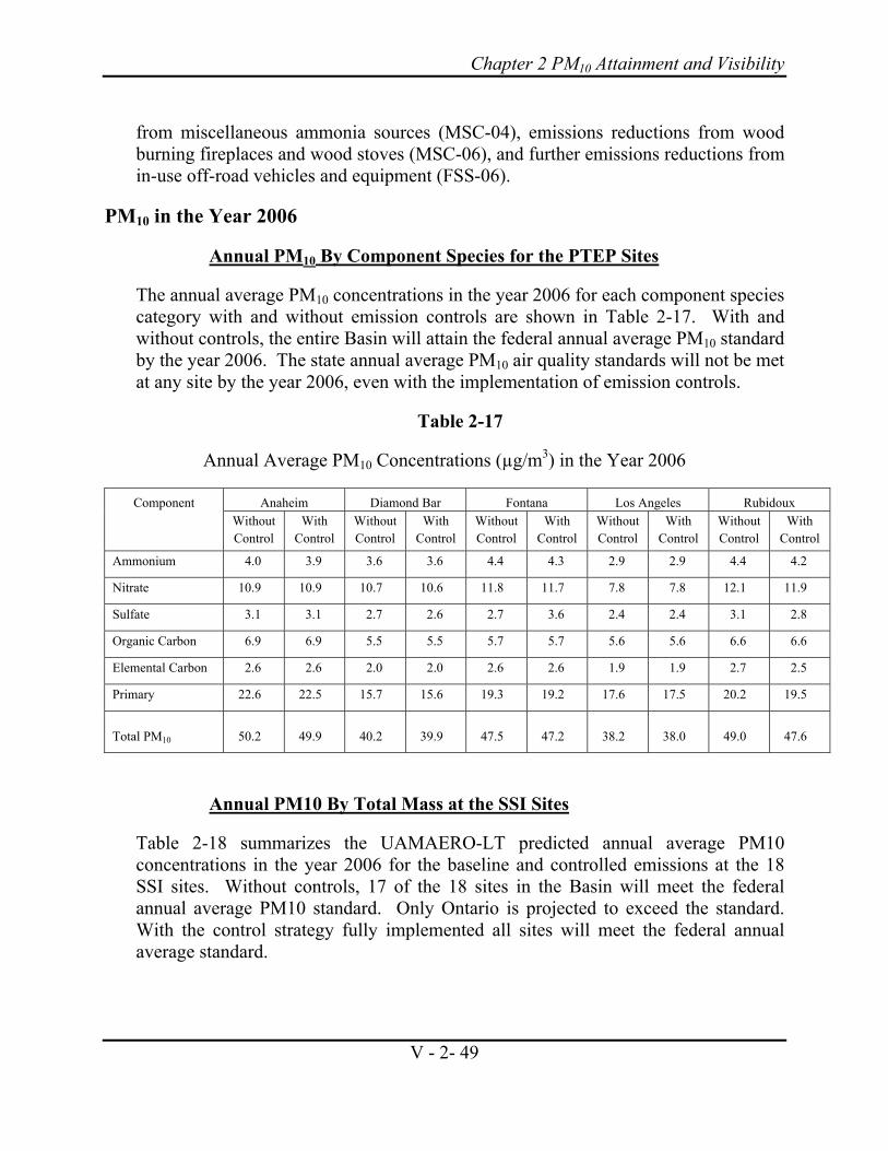
Chapter 2 PM10 Attainment and Visibility
V - 2- 49
from miscellaneous ammonia sources (MSC-04), emissions reductions from wood burning fireplaces and wood stoves (MSC-06), and further emissions reductions from in-use off-road vehicles and equipment (FSS-06).
PM10 in the Year 2006
Annual PM10 By Component Species for the PTEP Sites
The annual average PM10 concentrations in the year 2006 for each component species category with and without emission controls are shown in Table 2-17. With and without controls, the entire Basin will attain the federal annual average PM10 standard by the year 2006. The state annual average PM10 air quality standards will not be met at any site by the year 2006, even with the implementation of emission controls.
Table 2-17
Annual Average PM10 Concentrations (µg/m3) in the Year 2006
Anaheim Diamond Bar Fontana Los Angeles Rubidoux Component Without Control
With Control
Without Control
With Control
Without Control
With Control
Without Control
With Control
Without Control
With Control
Ammonium 4.0 3.9 3.6 3.6 4.4 4.3 2.9 2.9 4.4 4.2
Nitrate 10.9 10.9 10.7 10.6 11.8 11.7 7.8 7.8 12.1 11.9
Sulfate 3.1 3.1 2.7 2.6 2.7 3.6 2.4 2.4 3.1 2.8
Organic Carbon 6.9 6.9 5.5 5.5 5.7 5.7 5.6 5.6 6.6 6.6
Elemental Carbon 2.6 2.6 2.0 2.0 2.6 2.6 1.9 1.9 2.7 2.5
Primary 22.6 22.5 15.7 15.6 19.3 19.2 17.6 17.5 20.2 19.5
Total PM10 50.2 49.9 40.2 39.9 47.5 47.2 38.2 38.0 49.0 47.6
Annual PM10 By Total Mass at the SSI Sites
Table 2-18 summarizes the UAMAERO-LT predicted annual average PM10 concentrations in the year 2006 for the baseline and controlled emissions at the 18 SSI sites. Without controls, 17 of the 18 sites in the Basin will meet the federal annual average PM10 standard. Only Ontario is projected to exceed the standard. With the control strategy fully implemented all sites will meet the federal annual average standard.

Final 2003 AQMP Appendix V: Modeling and Attainment Demonstrations
V - 2- 50
UAMAERO-LT Grid-Level Simulation: 2006 Controlled Emissions
Figure 2-23 presents the 2006 UAMAERO-LT grid-level analysis for the controlled emissions scenario. With controls in place, all but 13 grid cells in the Basin are projected to have annual concentrations that will meet the federal standard. Five of the grid cells are located in Los Angeles and Orange counties in areas that experience heavy traffic and are impacted by paved road dust. One grid cell is located on the Basin boundary (in LA County near Acton) that appears to have emissions (from controlled burning activities) that are improperly distributed. The remaining seven grid cells are located in Basin portions of San Bernardino and Riverside Counties in areas heavily impacted by fugitive wind blown dust, construction dust and paved road dust.
The following section provides a weight of evidence discussion addressing the uncertainties in the primary dust emissions and their impact to the grid-level UAMAERO-LT 2006 future year PM10 prediction.
Table 2-18
UAMAERO-LT Predicted Annual Average PM10 Concentrations for Each SSI Site
Location 2006 Baseline Predicted Annual Average
Concentration (µg/m3)
2006 Controlled Predicted Annual Average
Concentration (µg/m3)
2006 Controlled Percentage of State
Standard
Central LA 38.2 38.0 194
Hawthorne 29.6 29.3 147
N. Long Beach 42.7 42.2 211
Burbank 35.3 35.1 176
Azusa 37.1 37.0 185
Pomona/Diamond Bar 40.2 39.9 200
Santa Clarita 36.8 36.7 184
Anaheim 50.2 49.9 250
El Toro 41.9 41.5 208
Norco 46.0 45.7 229
Rubidoux 49.0 47.6 238
Perris 38.7 38.4 192
Banning 18.1 18.0 90
Ontario 50.9 50.2 251
Fontana 47.5 47.2 236
San Bernardino 47.0 45.8 229
Redlands 33.8 33.4 167
Crestline 39.0 38.4 192

Chapter 2 PM10 Attainment and Visibility
V - 2- 51
Figure 2-23
UAMAERO-LT Grid-Level Simulation: 2006 Controlled Emissions (Grid Cell Predicted Concentrations in µg/m3 )
2006 UAMAERO-LT Hot Spot Grid Weight of Evidence Analysis
Figure 2-24 presents the 2006 UAMAERO-LT grid-level simulation depicting only the 13 "hot spot" grid cells. Table 2-19 lists the individual grids that had concentrations predicted by UAMAERO-LT that exceeded the federal standard for the 2006 controlled emissions scenario. Model predictions for the six species categories and total mass are presented. The Grids are sorted geographically into three general sub regions: LA-Orange Counties and Riverside-Basin San Bernardino Counties. Table 2-20 lists the ARB specified PM10 emissions source categories that were the major contributors to PM10 in the "hot spot" grid cells. Tables 2-21 through 2-22 present the top contributing PM10 emissions categories for each grid in the three groupings of cells.
In the L.A.-Orange Counties grouping the federal standard is predicted to be exceeded by a maximum of 4.1 µg/m3 (with the exception of grid cell [21,32] which is discussed later). The "other" or primary category is predicted to be between 19.8 and 24.7 µg/m3, an average of 22.3 µg/m3. The average predicted primary contribution in these grids is roughly 7 µg/m3 higher than the average observed primary component measured in 1995 at the Central L.A. and Anaheim PTEP sites.

Final 2003 AQMP Appendix V: Modeling and Attainment Demonstrations
V - 2- 52
Figure 2-24
UAMAERO-LT "Hot Spot" Grid Cells: 2006 Controlled Emissions (Grid Cell Predicted Concentrations in µg/m3 )
As presented in Table 2-21 the major contributing emissions source categories to L.A.-Orange Counties grouping are paved road dust, construction dust and off-road construction diesel equipment. Given that paved road dust on average contributed at least 9 µg/m3 to the primary category and that the emissions are estimated to be doubled the actual for this area of the Basin. As a consequence, it is most probable that with accurate emissions estimate of paved road dust, the predicted annual average concentrations would be at least 4.5 µg/m3 lower and would meet the federal standard. Uncertainties in the placement of construction dust and off-road equipment emissions most likely would lower the predicted concentration further.
Projected 2006 PM10, VOC, NOx and CO emissions for all of L.A. County's waste burning and disposal through forest management were inappropriately specified through a surrogate to grid cell (21,32). This accounts for the high predicted concentrations of primary, elemental carbon and organic carbon. The emissions should have been distributed over several grid cells in the Angeles National Forest, in areas with limited traffic, construction or other source of emissions. With the proper allocation of emissions, cell (21,32) would most likely meet the federal standard.

Chapter 2 PM10 Attainment and Visibility
V - 2- 53
Table 2-19
2006 UAMAERO-LT Predicted Hot Spot Grid Cells
Grid Predicted Mass (µg/m3) XX YY NH4 NO3 SO4 OC EC OTHER TOTAL
L.A.-Orange Counties 18 24 4 11.6 2.9 7.1 2.6 22.3 50.5 21 32 2 6.8 2.3 25.5 9.3 15.4 61.3 23 15 6.1 8.6 10.5 5 4.8 19.8 54.8 29 15 3.9 10.6 3.3 7 3.3 24.2 52.2 29 16 4 11.1 3.1 7.2 2.7 23.1 51.2 30 15 4 11.5 3 7.2 2.5 24.7 53
Riverside-Basin San Bernardino Counties 35 20 4.8 12.4 4.2 6.7 2.8 21.6 52.4 36 16 4.4 12.7 2.9 6.4 7.7 31.9 65.9 36 19 4.9 13 3.8 6.5 3.1 21.4 52.7 36 20 5.5 12.5 6 6.6 4.9 27.9 63.4 36 21 5.3 11.5 6.4 5.5 3.6 20.8 53 37 17 4.4 13.2 2.6 7 2.4 22.1 51.7 39 20 5.1 12.2 5 6.5 3 22.2 53.9
In the Riverside-Basin San Bernardino Counties grouping 5 of the 7 grid cells have annual average concentrations within 2.5 µg/m3 of the federal standard. Two grid cells (36,16) and (36,20) have predicted annual average concentrations above 63 µg/m3. Primary paved road dust and dust from construction and demolition activities account for the bulk of the primary PM10 emissions to the five grid cells that had predicted annual average concentrations with 2.4 µg/m3 of the standard. From the sensitivity analysis previously discussed, paved road dust typically contributes between 6 to 8 µg/m3 to annual average concentration at the Riverside and San Bernardino sites, respectively. Over-estimation of the paved road dust PM10 emissions by 3 µg/m3 is consistent with the estimation for the west Basin and that adjustment alone would bring the five sites within the federal standard. Uncertainties in the surrogates used to allocate construction and demolition dust associated and the expected construction growth also contribute to potentially lower annual average concentrations at those grid cells.

Final 2003 AQMP Appendix V: Modeling and Attainment Demonstrations
V - 2- 54
Table 2-20
PM10 Emissions Source Categories for 2006 Hot Spot Grid Cells
Source Category
Source Description
46987 Mineral Processes Other (Miscellaneous) Processes
47274 Waste Burning and Disposal -- Forest Management
47340 Farming Operations -- Cattle Feed Lots
47357 Construction and Demolition -- Building Construction Dust Residential
47365 Construction and Demolition -- Building Construction Dust Commercial
47373 Construction and Demolition -- Building Construction Dust Industrial
47381 Construction and Demolition -- Road Construction Dust
47399 Road Dust - Unpaved Road Travel Dust - City and County Roads
54551 Construction and Demolition -- Building Construction Dust Institutional
60418 Other-Commercial Charbroiling
82123 Residential Fuel Combustion-Wood Combustion-Fireplaces
83337 Fugitive Wind Blown Dust -Agricultural Lands
83352 Fugitive Wind Blown Dust - Unpaved Roads
83618 Road Dust - Paved Entrained Road Dust - Freeways
83626 Road Dust - Paved Entrained Road Dust - Major Roads
83634 Road Dust - Paved Entrained Road Dust - Collector Streets
83642 Road Dust - Paved Entrained Road Dust - Local Streets
84863 Fugitive Wind Blown Dust - Pasture Lands
89078 Off-Road Diesel Equipment

Chapter 2 PM10 Attainment and Visibility
V - 2- 55
Table 2-21
2006 Hot Spot Grid Cells Ventura, L.A. and Orange County:
PM10 Emissions (KG/Day) By Source Category
Grid (xx,yy) Source Category 1824 2315 2915 2916 3015 2132
83618 135 265 322 401 339 0 47274 0 0 0 0 0 1965 83626 281 180 242 158 144 0 83642 160 104 136 157 197 0 47365 45 28 204 135 135 0 89078 48 4 23 51 31 0 60418 42 28 47 56 49 0 47357 28 21 38 36 39 0 54551 24 15 32 22 21 0
Table 2-22
2006 Hot Spot Grid Cells Riverside and San Bernardino County: PM10 Emissions (KG/Day) By Source Category
Grid (xx,yy) Source
Category 3520 3616 3619 3620 3621 3717 3920 83642 138 83 112 103 30 117 150 83626 251 60 126 69 134 120 148 83618 0 143 79 127 102 100 123 83352 436 6 5 3 4 15 4 47365 70 0 26 46 160 16 0 47373 120 0 15 117 53 0 24 47357 18 0 72 64 50 48 0 60418 7 15 17 0 0 77 35 83634 11 16 23 25 13 34 11 54551 9 15 0 8 5 59 5 47340 0 0 73 0 3 0 0
Grid cell (36,16) is particularly impacted by fugitive dust emissions from unpaved roads together with large contributions from paved road dust and construction and demolition dust as well. Approximately 5.5 percent of all Basin fugitive dust emissions from unpaved roads (8.7 TPD) are located in that one grid cell. Interestingly, the bulk of grid cell (36,16) resides in the City of Corona in a

Final 2003 AQMP Appendix V: Modeling and Attainment Demonstrations
V - 2- 56
developed portion of the city that includes a shopping plaza and a maintained golf course. As a consequence, the amount of particulate emissions from unpaved roads may have been misallocated to that grid. Without the fugitive unpaved road dust emissions, the total listed in Table 2-22 for grid cell (36,16) are comparable with those of the other five grid cells (except 36,20). In addition, while future construction growth is reasonable, uncertainties exist in the estimated amount of 2006 construction, given the level of current development of the area. With adjustments for paved fugitive unpaved road dust, paved road dust and construction emissions it is likely that grid cell (36,16) would meet the 50.4 µg/m3 threshold.
Grid cell (36,20) has a significant contribution from paved road dust and construction dust to its major particulate emissions and the predicted primary impact to that grid should be weighted by the uncertainties in those emissions estimates. Grid cell (36,20) is also directly downwind of the cell 35,19 which has one of the highest concentrations of cattle feed lot emissions (0.77 TPD) in the Basin. The cattle feed lot emissions were used as a surrogate for dairy farm dust emissions. There is huge amount of uncertainty in these emissions since dairy farms are typically well irrigated and do not raise the same amount of dust as cattle feed lots. In addition, the area of grid cell (35,19) is rapidly being transformed from dairy farms to warehouse distribution centers. It is unlikely that in 2006, many of the dairy farms will continue to be in operation.
The results of the "hot-spot" grid cell analysis indicate that the UAMAERO-LT simulation for 2006 meets the federal standard when localized anomalies in primary emissions specification and systematic over-estimation of the paved road dust estimates are identified and accounted.
Maximum 24-Hr Average PM10
The maximum 24-hour average PM10 concentrations in the year 2006 for each site with and without emission controls are shown in Table 2-23 Los Angeles will meet the federal 24-hour average PM10 standard without emission controls in 2006. With emission controls, the entire Basin will attain the federal 24-hour average PM10 standard of 150 µg/m3 in 2006.
None of the sites in the Basin will meet the state maximum 24-hour average PM10 standard of 50 µg/m3 in the year 2006, even with the proposed emission controls.

Chapter 2 PM10 Attainment and Visibility
V - 2- 57
Table 2-23
Maximum 24-hr Average PM10 Concentrations (µg/m3) in the Year 2006
Anaheim Diamond Bar Fontana Los Angeles Rubidoux
Without Control
With Control
Without Control
With Control
Without Control
With Control
Without Control
With Control
Without Control
With Control
Total PM10 138.5 137.5 124.4 123.3 129.2 128.4 117.8 116.7 155.6 150*
* With EPA Rounding Convention [40 CFR Part 50, Appendix K]
PM10 in the Year 2010
Annual PM10
The annual average PM10 concentrations in the year 2010 for each PM10 species with and without emission controls are shown in Table 2-24. With and without controls, the all sites will meet the federal annual average PM10 standard. However, even with controls in place, none of the sites will meet the state annual average PM10 standard in 2010, regardless of the control option selected.
TABLE 2-24 Annual Average PM10 Concentrations (µg/m3) in the Year 2010
Anaheim Diamond Bar Fontana Los Angeles Rubidoux
Control Control Control Control Control
Component
Base
Opt-1 Opt-2
Base
Opt-1 Opt-2
Base
Opt-1 Opt-2
Base
Opt-1 Opt-2
Base
Opt-1 Opt-2
Ammonium
3.8 3.2 3.3 3.5 3.0 3.1 4.4 3.7 3.8 2.8 2.4 2.5 4.3 3.5 3.5
Nitrate
10.3 7.7 8.4 10.1 7.8 8.2 11.3 8.9 9.0 7.4 5.9 6.2 11.6 9.1 9.2
Sulfate
3.2 3.2 3.2 2.7 2.7 2.7 3.9 3.9 3.8 2.6 2.4 2.4 3.3 3.0 2.9
Organic Carbon
6.7 6.0 6.2 5.4 4.8 5.0 5.8 5.6 5.5 5.4 4.9 5.0 6.6 6.3 6.4
Elemental Carbon
2.6 2.5 2.5 2..1 2.0 2.0 2.8 2.7 2.7 2.0 1.9 1.9 2.7 2.4 2.5
Primary
23.0 22.8 22.8 16.0 15.9 15.9 20.3 20.2 20.2 17.7 17.5 17.5 21.5 20.7 20.7
Total PM10
49.7 45.4 46.4 39.8 36.3 36.8 48.4 44.7 45.0 37.8 35.3 35.7 50.1 45.0 45.2

Final 2003 AQMP Appendix V: Modeling and Attainment Demonstrations
V - 2- 58
Maximum 24-Hr Average PM10
The maximum 24-hour average PM10 concentrations in the year 2010 for each site with and without emission controls are shown in Table 2-25. All sites will meet the federal 24-hour average PM10 standard with and without emission controls in 2010. None of the sites in the Basin will meet the state maximum 24-hour average PM10 standard in the year 2010, even with the proposed emission controls.
TABLE 2-25 Maximum 24-Hour Average PM10 Concentrations (µg/m3) in the Year 2010
Anaheim Diamond Bar Fontana Los Angeles Rubidoux
Control Control Control Control Control
Component
Base
Opt-1 Opt-2
Base
Opt-1 Opt-2
Base
Opt-1 Opt-2
Base
Opt-1 Opt-2
Base
Opt-1 Opt-2
Total PM10 129.1 110.8 115.8 113.5 93.8 99.4 124.9 113.2 116.2 107.2 88.4 93.7 148.7 132.9 137.1
PM2.5 in the Year 2010
Annual PM2.5
The annual average PM2.5 concentrations in the year 2010 for each PM2.5 species with and without emission controls (both options) are shown in Table 2-26. The future year PM2.5 is presented to provide an assessment as to the amount of additional emissions reductions that will be required to meet the federal PM2.5 standard when the propose 2014 attainment date is implemented. With and without controls, the predicted PM2.5 concentrations for Basin in 2010 will exceed the federal PM2.5 standard. For the five key sites, annual average PM2.5 concentrations are predicted to exceed the federal standard by a minimum of 31 percent at Central L.A. to a high 89 percent at Fontana.

Chapter 2 PM10 Attainment and Visibility
V - 2- 59
Table 2-26
Annual Average PM2.5 Concentrations (µg/m3) in the Year 2010
Anaheim Diamond Bar Fontana Los Angeles Rubidoux
Control Control Control Control Control
Component
Base
Opt-1 Opt-2
Base
Opt-1 Opt-2
Base
Opt-1 Opt-2
Base
Opt-1 Opt-2
Base
Opt-1 Opt-2
Ammonium 3.4 2.9 3.0 3.2 2.7 2.8 4.0 3.4 3.4 2.5 2.2 2.3 3.9 3.2 3.2
Nitrate 7.6 5.7 6.2 7.5 5.8 6.1 8.4 6.6 6.7 5.5 4.4 4.6 8.6 6.7 6.8
Sulfate 2.6 2.6 2.6 2.2 2.2 2.2 3.2 3.2 3.1 2.1 2.0 2.0 2.7 2.5 2.4
Organic Carbon
4.8 4.1 4.3 4.0 3.5 3.6 4.3 4.1 4.0 3.8 3.4 3.5 5.1 4.8 4.9
Elemental Carbon
2.3 2.2 2.2 1.9 1.8 1.8 2.5 2.4 2.4 1.8 1.7 1.7 2.3 2.1 2.2
Primary 6.8 6.7 6.7 5.3 5.2 5.2 7.6 7.5 7.5 5.4 5.3 5.3 7.5 7.0 7.0
Total PM2.5 27.7 24.3 25.1 24.1 21.3 21.7 29.9 27.0 27.2 21.1 19.1 19.4 30.2 26.3 26.4
Maximum 24-Hr Average PM2.5
The maximum 24-hour average PM2.5 concentrations in the year 2010 for each site with and without emission controls are shown in Table 2-27. None of the sites will meet the federal 24-hour average PM2.5 standard (65 µg/m3) without emission controls in 2010. With emission controls, the federal 24-hour average PM2.5 standard is predicted to be attained at Anaheim, Los Angeles and Rubidoux (both control options) and at Diamond Bar for control option-1. The PM2.5 standard is not attained at Fontana, regardless of control option selected.
TABLE 2-27 Maximum 24-Hour Average PM2.5 Concentrations (µg/m3) in the Year 2010
Anaheim Diamond Bar Fontana Los Angeles Rubidoux
Control Control Control Control Control
Component
Base
Opt-1 Opt-2
Base
Opt-1 Opt-2
Base
Opt-1 Opt-2
Base
Opt-1 Opt-2
Base
Opt-1 Opt-2
Total PM10 76.5 59.1 63.9 84.9 65.0 70.6 79.3 68.4 71.3 67.8 52.2 56.5 76.8 64.4 67.7

Final 2003 AQMP Appendix V: Modeling and Attainment Demonstrations
V - 2- 60
PM10 in the Year 2010 With Alternative Control Options
As part of the California Environmental Quality Act (CEQA) requirements, four alternatives to the two proposed control plan options for 2010 were evaluated for both the ozone and PM10 attainment plans. These options include:
• Alt.-1: No Project Taking Place.
• Alt.-2b: Lower VOC (~ 250 TPD) with Control Option-2.
• Alt.-3: Lower VOC (~250 TPD) with Control Option-1.
• Alt.-4 Least amount of Toxic Emissions Option. .
Annual and 24-hour maximum concentration PM10 simulations for total mass were conducted for the alternative emissions scenarios. The results of the annual simulations are presented in Table 2-28. The results of the 24-hour maximum concentration simulations are presented in Table 2-29.
All of the alternative controls strategies will result in the both the annual and 24-hour maximum federal PM10 standards to be attained in 2010 at all sites.
Table 2-28
Alternative Emissions Control Scenarios: Predicted Annual Average PM10 Concentrations (µg/m3) in the Year 2010
Scenario Anaheim Diamond Bar
Fontana Los Angeles Rubidoux
Alt.-1 47 38 45 36 47
Alt.-2b 46 36 45 36 45
Alt.-3 45 36 44 35 44
Alt.-4 45 36 45 35 45

Chapter 2 PM10 Attainment and Visibility
V - 2- 61
TABLE 2-29 Alternative Emissions Control Scenarios: Predicted 24-Hour Average Maximum PM10
Concentrations (µg/m3) in the Year 2010
Scenario Anaheim Diamond Bar
Fontana Los Angeles Rubidoux
Alt.-1 123 106 120 101 142
Alt.-2b 115 99 116 93 136
Alt.-3 110 93 113 88 132
Alt.-4 109 91 112 86 131
CONCLUSIONS
In the year 2006, and continuing through 2010, PM10 concentrations will be reduced to levels such that the entire Basin will comply with both federal PM10 standards, annual average and maximum 24-hour average (summarized in Figures 2-25 and 2-26, respectively) with the proposed emission controls. However, neither of the state PM10 standards can be met by 2006 or 2010 with the proposed emission controls. Further emission controls will be necessary to meet the state PM10 standards.
As part of the federal Clean Air Act requirements for the PM10 attainment demonstration, interim milestone emission reduction targets must be provided for every three years to the attainment year.

Final 2003 AQMP Appendix V: Modeling and Attainment Demonstrations
V - 2- 62
01020304050607080
Central LA Anaheim DiamondBar
Fontana Rubidoux
Conc
entra
tion
(ug/
m3)
1995-Baseline 2006-Baseline 2006-Controlled2010-Baseline 2010-Control Opt.-1 2010-Control Opt.-2
FIGURE 2-25 Future Projected Annual Average PM10 for the Baseline and Control Emissions Scenarios
0
50
100
150
200
250
Central LA Anaheim Diamond Bar Fontana Rubidoux
Con
cent
ratio
n (u
g/m
3)
1995-Baseline 2006-Controlled 2010-Control Opt.-1
FIGURE 2-26 Future Projected Maximum 24-Hour Average PM10 for the Baseline and Control
Emissions Scenarios

Chapter 2 PM10 Attainment and Visibility
V - 2- 63
VISIBILITY
Background
Visibility impairment plays an important role in the public’s perception of the general state of air quality, since it is one of the most obvious indicators of air pollution. In 1969, California promulgated an ambient air quality standard for “visibility-reducing particles,” limiting the concentration of these particles to an amount which would not reduce the visibility below 10 miles when the relative humidity was less than 70 percent. On January 13, 1989, the California Air Resources Board (ARB) established a new visibility standard based on instrumental determination of atmospheric extinction coefficient. Effective in October 1989, the new standard states that the concentration of “visibility-reducing particles” violates the standard when it produces an extinction coefficient greater than 0.23 per kilometer (equivalent to visibility less than 10 miles) with relative humidity less than 70 percent, averaged over the period from 10:00 am to 6:00 pm, Pacific Standard Time (ARB, 1989). There is no requirement to comply with the state visibility standard by a specified date; however, future-year visibility is estimated to illustrate the progress toward the attainment of the state standard.
Visibility Modeling
To establish the most reasonable control strategy to meet the visibility standard in the future, a relationship between visibility and concentrations of visibility reducing particles must be established. This, in turn, requires visibility modeling techniques to identify sources of visibility reducing particles and to quantify their impacts.
The total atmospheric light extinction can be broken down into four basic components: scattering of light by particles, absorption of light by particles, absorption of light by gases, and scattering of light by gases (Rayleigh scattering). In general, total light extinction is dominated by scattering of light due to particles, with light absorption by particles being second in importance. The components other than scattering of light by particles have been well-characterized by theory or from previous studies. Therefore, light extinction by particle scattering is normally estimated either by visibility modeling or by direct measurement.
Multiple linear regression is a statistical tool commonly used for characterizing the relationship between visibility and ambient air quality of the visibility reducing particles. When atmospheric light extinction due to particle scattering is regressed on concentrations of visibility reducing particles, the regression coefficients represent the extinction efficiency due to particle scattering (extinction per unit concentration) for each air pollutant species.

Final 2003 AQMP Appendix V: Modeling and Attainment Demonstrations
V - 2- 64
Multiple linear regression was employed in the 1991 AQMP to develop empirical predictive equations. Empirical visibility model developed in the 1991 AQMP for Riverside were utilized in the current AQMP analysis to estimate future visibilities with new future-year (2006, and 2010) organic carbon concentrations, sulfate, and nitrate concentrations which were obtained from the UAMAERO-LT model. Details of the statistical analysis used to develop the empirical predictive equations can be found in Technical Report V-G of the 1991 AQMP.
Prior Visibility Modeling Results
In the 1991 AQMP, the regression analysis resulted in several sets of extinction efficiencies for light scattering by particles for Riverside (Rubidoux station) and four additional measurement locations. Combining extinction efficiencies for light scattering by particles with the empirical expressions for the other light extinction component produces a series of empirical predictive equations. Empirical predictive equations relate light extinction to concentrations of visibility reducing air pollutants and have the following form:
bext = Summation ( bi . Ci )+ bRAY
where bi = extinction efficiency for ith species (10-4 m-1/µg/m3 or 10-4 m-1/pphm)
Ci = mean concentration for ith species (µg/m3 or pphm)
bRAY = extinction due to Rayleigh scattering in the Basin (10-4 m-1)
Table 2-30 is a summary of the 1991 AQMP results, showing the extinction efficiency, bi, for Riverside. (The extinction efficiency, bi, for the other locations analyzed in the 1994 AQMP can be found in 1994 AQMP, Technical Report V-C).
A baseline light extinction budget was determined for each empirical predictive equation using the mean measured values of the air quality components for the baseline year 1986. The light extinction budget for Riverside during the baseline emission year is summarized in Table 2-31. These show the percent contribution to total extinction from each component for each equation.
At Riverside light scattering by particles accounts for up to 87 percent of the total light extinction with secondary nitrate and carbon particles being dominant.

Chapter 2 PM10 Attainment and Visibility
V - 2- 65
TABLE 2-30 Riverside Extinction Efficiencies, bi, Defining Alternate Sets of Empirical Predictive
Equations for Light Extinction
Visibility-Reducing Alternate Equations1 Species Units 1 2 3 4
Riverside SULF (10-4 m-1/µg/m3) b1
NITR (10-4 m-1/µg/m3) b2 0.070 0.075 IONS (10-4 m-1/µg/m3) b3 0.055 0.058 OC (10-4 m-1/µg/m3) b4 0.104 0.089 CRBN (10-4 m-1/µg/m3) b5 0.062 0.053 EC (10-4 m-1/µg/m3) b6 0.119 0.119 0.119 0.119 NO2 (10-4 m-1/pphm) b7 0.033 0.033 0.033 0.033 molecules (10-4 m-1) bRAY 0.114 0.114 0.114 0.114
TABLE 2-31 Current Light Extinction Budgets for Each Alternate Empirical
Predictive Equation at Each Measurement Location2 (in percent of total light extinction)
Alt ______________b sp ______________ Location Eq. SULF NITR IONS OC CRBN bap bag bRAY
Riverside 1 58 29 8 2 3 2 66 21 8 2 3 3 62 25 8 2 3 4 62 25 8 2 3
1 Alternate equations in the set of empirical predictive equations defined for each measurement location. 2 Based on mean annual average concentrations derived from 1986 measurements.

Final 2003 AQMP Appendix V: Modeling and Attainment Demonstrations
V - 2- 66
Predicted Future Air Quality
Future air quality levels are needed to estimate future visual air quality. The concentrations of the inorganic particulate matter species (sulfate and nitrate) for future years 2006, and 2010 are taken from the results of the UAMAERO-LT modeling analysis.
Future concentrations of particulate organic carbon, particulate elemental carbon, and gaseous NO2 are estimated from the mean annual concentrations measured during 1986 using linear rollback. Linear rollback assumes that the change in pollutant levels at any location in the Basin is linearly proportional to the expected change in basin-wide emission loading.
Future NO2 concentrations are estimated from NOx emissions, particulate organic carbon from emissions of VOCs and particulate elemental carbon from diesel particulate emissions. Natural background concentrations for each of these are assumed to be negligible for this analysis.
Table 2-32 gives the basin-wide emission totals for VOC, NOx, SOx and diesel particulate matter. Totals are given for 1990 (the baseline emission year) and for future years 2006, and 2010 with two emission control scenarios: baseline (no additional controls) and controlled.
TABLE 2-32 Baseline and Future Controlled Emissions (tons per day)
Pollutant 1990 2006b 2010b 2006c 2010c
VOC 1780 689 615 674 295 NOx 1592 943 771 935 543
SOx 98 60 60 57 59
Diesel Particulate 33 20 18 20 12 b without AQMP control strategies c with AQMP control strategies
Estimated future baseline and controlled levels for all pollutant species that affect visibility are shown in Tables 2-33.

Chapter 2 PM10 Attainment and Visibility
V - 2- 67
TABLE 2-33 Riverside Air Quality Levels for the Years 2006 and 2010
Future Baseline and Controlled (2010 Opt.-1)
Component Units Baseline Controlled
2006 SULF
1 µg/m3 5.0 4.5
NITR1 µg/m3 19.6 19.3
IONS µg/m3 24.6 23.8 OC
2 µg/m3 5.5 5.5
EC2 µg/m3 2.7 2.5
CRBN µg/m3 9.3 9.1 NO2
2 pphm 1.5 1.5
2010 SULF
1 µg/m3 5.3 4.9
NITR1 µg/m3 18.8 14.7
IONS µg/m3 24.1 19.6 OC
2 µg/m3 5.5 5.3
EC2 µg/m3 2.7 2.4
CRBN µg/m3 9.3 8.7 NO2
2 pphm 1.3 0.9
Future Visibility Projections
Riverside Future Mean Visibility
Tables 2-34 and 2-35 compare the predicted future visibility with the current levels based on measurements. The results for the baseline emission scenario (no further emission controls) are shown in Table 2-34 and the results for the controlled emission scenarios are shown in Table 2-35. Each table shows the predicted annual average light extinction coefficients compared to the total light extinction coefficient derived from 1986 measurements and the mean visual range estimated from the measured and predicted extinction coefficients. Figure 2-27 illustrates the improvement in visibility in terms of the annual visual range for both emission control scenarios.

Final 2003 AQMP Appendix V: Modeling and Attainment Demonstrations
V - 2- 68
TABLE 2-34 Projected Future Visibility, Baseline without Future Controls
Year Alt. Eq.1 Total Light Extinction Coefficient (10-4 m-1)
Calculated Visual Range (miles)
Baseline 3.9 4.8
2006 1 2.328 8.0 2 2.429 7.7 3 2.406 7.7 4 2.531 7.4
2010 1 2.292 8.1 2 2.363 7.9 3 2.368 7.9 4 2.461 7.6
TABLE 2-35 Projected Future Visibility, With Controls
Year Alt. Eq.1 Total Light Extinction Coefficient (10-4 m-1)
Calculated Visual Range (miles)
Baseline 3.9 4.8
2006 1 2.260 8.2 2 2.382 7.8 3 2.324 8.0 4 2.470 7.5
2010 1 1.973 9.4 2 2.006 9.3 3 2.026 9.2 4 2.073 9.0
1 Alternate equations in the set of predictive empirical equations defined for each measurement location.

Chapter 2 PM10 Attainment and Visibility
V - 2- 69
FIGURE 2-27
Annual Average Daytime Visibility Projections, Miles
For the baseline emission control scenario, there is a decrease in the total extinction coefficient from the baseline to the year 2010. The visual range will subsequently increase by about 3.0 miles by 2006 to 7.7 miles and increase an additional 0.2 miles to 7.9 miles in 2010.
For the controlled emission scenario, the total extinction coefficient is reduced to less than half of the base year value. Corresponding visual range improves from 4.8 miles in the base year to 9.3 miles in 2010. The predicted future visibilities are consistent with the observed annual average visual range in areas influenced by marine air (with the attendant marine haze). Without significant air pollution sources, median mid-day visibilities along the California coast are generally less than 25 miles (Trijonis, 1980).
Future Light Extinction Budgets at Riverside
Table 2-36 compares the baseline and future projected light extinction budgets determined from one of the alternate empirical equations for each location to illustrate changes in the importance of each pollutant component to overall light extinction. These changes result from alterations in the future pollutant mix and in the spatial distribution of sources.
0
2
4
6
8
10
1986 2006 2010
Visi
bilit
y (M
iles)
Baseline Control
0
2
4
6
8
10
1986 2006 2010
Visi
bilit
y (M
iles)
Baseline Control

Final 2003 AQMP Appendix V: Modeling and Attainment Demonstrations
V - 2- 70
Table 2-36
Comparison of Baseline and Future Projected Light Extinction Budgets for Riverside (% contribution)
Baseline Controlled Component 1986 2006 2010 2006 2010
NITR 60 56 56 57 51 OC 29 24 24 24 27 EC 8 13 14 12 14 NO2 2 2 2 2 1 RAY. 3 5 5 5 6
The light extinction budget for Riverside changes very little for the future baseline emission cases except for the following: (1) nitrate remains the major contributor but its contribution decreases; and (2) elemental carbon contributions increase by approximately one third from the base year then remain constant through 2010.
The projected light extinction budgets for the years 2006 and 2010 with the controlled emission scenarios are relatively equivalent to the baseline budgets but show changes from the 1986 baseline, most notably from the smaller contribution by nitrate and a nominal increase due to elemental carbon.
CONCLUSIONS
In general, visibility is a tangible indicator of air quality. Particulate matter in the atmosphere causes not only visibility reduction but also adverse health effects. Visibility in the Basin has shown improvement over the last 30 years; however, the California state visibility standard continues to be violated throughout the Basin. Visibility impairment in the Basin is primarily due to the scattering and absorption of light by fine particles suspended in the atmosphere.
Without emission controls, visibility is predicted to improve only marginally. With the proposed emission controls, annual average visibility will improve from a range of approximately 5.0 miles at Riverside to 7.7 miles by 2006 and to 7.9 miles by 2010. This level of improvement is consistent with visibilities experienced in the non-urban coastal areas of California that have little impact from man-made sources but are affected by marine haze.
Total extinction coefficient improves by approximately 50 percent by the year 2010 with the implementation of controls. This corresponds to an improvement in the annual average visual range from less than 5 to more than 9 miles at Riverside by 2010.

CHAPTER 3 REVISION TO THE 1997 OZONE ATTAINMENT DEMONSTRATION PLAN
Introduction Emissions Summary Episode Selection Modeling Methodology Model Validation Future Ozone Air Quality Projections Sensitivity Studies Summary and Conclusions


Chapter 3 Revision to the 1997 Ozone Attainment Demonstration Plan
V-3-1
INTRODUCTION
The 2003 AQMP Ozone Attainment Demonstration Plan to meet the federal 1-hour average standard (124 ppb) is presented in this chapter. The modeling Attainment Demonstration serves as a revision to the 1997 ozone Attainment Demonstration Plan (Ozone Plan) submitted to EPA as part of the California State Implementation Plan (SIP). The ozone modeling attainment demonstration relies on an established modeling system the Urban Airshed Model (UAM) with the Carbon Bond IV (CB-IV) mechanism (Morris and Myers, 1990) and two modeling episodes. The primary modeling episode used in the current analysis, August 5-6, 1997, occurred during the 1997 Southern California Ozone Study. This episode is one of several meteorological episodes that were intensively monitored through the field program. A second meteorological episode, August 27-28, 1987, that was previously used in the 1994 and 1997 AQMP ozone attainment demonstrations was included in the analysis to provide continuity between Ozone Plans. The base year for the ozone modeling demonstration and emissions inventory characterization is 1997.
Note, only August 5th and 6th of the 1997 meteorological episode are used in the ozone attainment demonstration. As discussed in Chapter 1, August 4, 1997 was considered a "ramp-up" day for the ozone simulation and as such was excluded from the attainment demonstration analysis. However, the meteorological fields generated for August 4, 1997 are included in the discussion of meteorological input preparation in a following section of this chapter. The meteorological fields are included in the discussion to support the overall evaluation of how well the modeled meteorological fields recreate the meteorological conceptual model defining the episode.
This chapter provides the background for the development of the components that contribute to the ozone modeling attainment demonstration. Included are discussions of the modeling tool selected for the demonstration, federal and state air quality standard requirements, and base and future year emissions. The selection and characterization of meteorological episodes and preparation of the ozone simulation model input is provided in detail. The analysis also provides the base year model validation and supporting statistical and graphical documentation.
Ozone air quality is projected using the UAM for the following future years: 2007 and 2010. The year 2007 is used in the discussion of federal attainment demonstration for the severe-17 Coachella Valley nonattainment area. The year 2010 was chosen for UAM modeling to demonstrate attainment of the federal ozone standard in the South Coast Air Basin. Additional analyses provide characterization of future year air quality for alternative emissions control strategies.

Final 2003 Appendix V: Modeling and Attainment Demonstrations
V-3-2
Model Selection
Projections of future air quality rely on the use of computer simulation models. The model used in the 2003 AQMP to project future ozone air quality and to determine the effectiveness of the proposed control strategies is the Urban Airshed Model (UAM) with the Carbon Bond IV (CB-IV) mechanism (Morris and Myers, 1990). The analysis uses UAM version 6.23 for the attainment demonstration. U.S. Environmental Protection Agency's (EPA) modeling guidelines recommends the use the UAM model for urban scale modeling simulations.
As previously discussed in Chapter 1, EPA's guidance also promotes the use of state-of-the-art modeling systems provided that they perform equal to or better than the reference model (UAM). As such, several additional candidate models were evaluated for use in the 2003 AQMP. The California Photochemical Grid Model (CALGRID) with the CB-IV and SAPRC99 chemical mechanisms as well as the Comprehensive Air Quality Model with Extensions (CAMx) also with CB-IV and SAPRC99 chemistry were extensively evaluated for inclusion in the ozone modeling attainment demonstration. The performance of CALGRID and CAMx to recreate the patterns of ozone in space and time exceeded those of UAM. Both CALGRID and CAMx met EPA's baseline model performance criteria for the critical geographical receptor area of the Basin, however, each model under predicted observed unpaired peak concentrations. In contrast the UAM predicted peak concentration essentially matched the unpaired observed peak concentration.
While no stated preference is made as to relative importance of the individual performance criteria used to evaluate the different models, the ability to recreate observed peak concentrations ranks high. The peak concentration represents the starting threshold from which emissions need to be reduced to meet the standard. Under prediction of the peak concentrations can lead to significant uncertainty in Basin carrying capacity estimation. Both CALGRID and CAMx, (each model using CB-IV and SAPRC99 chemistry), under predicted the base-year peak concentrations by more than 10 percent. This trend of under prediction of observed ozone was also demonstrated by the CAMx and CALGRID performance on a 2002 "mid-course" simulation analysis. Uncertainties in the application of the SAPRC99 chemistry and speciation of VOC from biogenic sources needed for the SAPRC99 chemistry further complicated the evaluation of the CALGRID and CAMx simulations.
For the 2003 AQMP, UAM has been selected as the primary modeling tool for the ozone attainment demonstration. The decision to use UAM rests on the model's ability to recreate the observed peak concentration, coupled with its performance on the "mid course" simulation and the District's extensive experience with UAM in prior AQMPs. The District is committed to moving towards the use of the state-of-the-science air quality simulation models. At this time, CALGRID/SAPRC99 model simulations show

Chapter 3 Revision to the 1997 Ozone Attainment Demonstration Plan
V-3-3
consistency with the UAM future year simulations. Unfortunately, the CAMx simulations do not show as much promise. If the issues with that have discussed here and in Chapter 1 are resolved prior to adoption of the final plan, a technical document addressing the CALGRID/SAPRC99 base and future year simulations will be appended to this document as supporting weight of evidence to the ozone attainment demonstration.
Federal 1-Hour Ozone Standard Requirements
Air quality modeling is required by both the federal Clean Air Act (CAA) and the California Clean Air Act (CCAA). Section 182(b)(1)(A) of CAA requires that moderate and above ozone nonattainment areas must reduce volatile organic compounds (VOC) and oxides of nitrogen (NOx) emissions sufficiently to attain the national ambient air quality standard for ozone and an attainment demonstration must be performed using photochemical grid modeling. According to Section 181(a)(1) of the CAA, ozone nonattainment areas are classified and given an attainment deadline based on their design values. Within the jurisdiction of the District are the South Coast Air Basin (Basin) and the Coachella Valley of the Salton Sea Air Basin (see Figure 3-1). The Basin is classified as an extreme ozone nonattainment area and therefore has an attainment deadline of November 15, 2010. The attainment demonstration for the Basin is the primary subject of this chapter. The Coachella valley is classified as a “severe-17” ozone nonattainment areas and therefore have an attainment deadline of November 15, 2005 with a two year extension to 2007.
The modeling domain used in the photochemical modeling analysis, also shown in Figure 3-1, encompasses the entire Basin, Ventura County, Antelope Valley (AVAQMD), San Diego County, the Coachella Valley, and portions of the Mojave Desert Air Quality Management District (MDAQMD) and Imperial County. Ventura county, classified as a severe ozone nonattainment area (attainment year: 2005), the Antelope Valley and Mojave Desert are classified as "severe-17" (attainment year: 2007), experience pollutant transport from the Basin, and at times is an upwind source of pollution.
California Requirements and Population Exposure
The CCAA requires the District to demonstrate reasonable progress towards achieving state ambient air quality standards in the Basin. The CCAA requires per-capita exposure reductions for the years 1994, 1997, and 2000, as compared to a 1986-88 base period. Overall per-capita exposure to ambient ozone must be reduced in accordance with the following schedule: 25 percent by 1994, 40 percent by 1997, and 50 percent by 2000.

Final 2003 Appendix V: Modeling and Attainment Demonstrations
V-3-4
To date, the Basin has not met the California 1-hour ozone standard (90 ppb) yet, ambient ozone air quality has greatly improved.
For the 2003 AQMP, the Regional Human Exposure model (REHEX) is used to determine per-capita exposure reductions based on observed ozone air quality. In previous plans, REHEX was coupled with the output of the UAM regional photochemical simulations to estimate future year population exposure to address the CCAA requirements. While the current ozone modeling attainment demonstration uses 1997 as a base year for the attainment demonstration, observational ozone data are available for the milestone years identified by the CCAA. The results of the REHEX per-capita population exposure analysis for the milestone years using the observed ozone air quality are presented in Table 3-1. In summary, the population exposure requirement defined by the CCAA has been achieved.
Figure 3-1
Southern California Modeling Domain Used in the Ozone Attainment Demonstration

Chapter 3 Revision to the 1997 Ozone Attainment Demonstration Plan
V-3-5
Table 3-1
CAAA Population Exposure Assessment
Period Per-Capita Ozone Exposure (pphm-hr)
Percent Improvement from 1986-1988
1986-1988 132.57 N/A 1994 50.16 62 % 1997 7.98 94 % 2000 4.61 97 %
EMISSIONS SUMMARY
Introduction
There are specific emission inventories developed for the photochemical modeling. The summer planning emission inventories developed for the historical years (1987, and 1997) and future planning years (baseline and controlled) are described in Appendix III. Baseline modeling inventories for the historical years (1987 and 1997) and the future years (2007, 2010, and 2020) are discussed next. Two emission projections are needed for each of the modeled future years. The first is the projected emissions assuming no further emission controls. These projections are commonly referred to as “baseline emissions” (e.g., 2010 baseline emissions), and reflect the emissions resulting from increases in population and vehicle miles traveled (VMT), as well as the implementation of all adopted rules and regulations up to November 30, 2002. The second emission projections reflect the implementation of the 2003 AQMP control measures on the future baseline emissions. For a detailed description of the 2003 AQMP control measures, the reader is referred to the main volume and Appendix IV.
The 1987 and 1997 historical year emissions are summarized first for the two ozone episodes used for attainment demonstration. This is followed by a discussion of the future-year baseline emission inventories. Finally the future-year emission inventories, assuming implementation of proposed control measures, are presented. Appendix III contains emission summary reports by source category for the historical base year, future baseline, and future controlled scenarios used in this modeling analysis. Attachments 4, 5, and 6 of this appendix contain an emissions summary report by source category for the future (2006 and 2010) controlled scenarios for the annual average inventory, and the 2010 controlled scenario for the planning inventory, respectively. It should be noted that the inventories reported here may be slightly different than those reported in the 2003 AQMP and Appendix III, since the inventories used for modeling reflect day-specific conditions.

Final 2003 Appendix V: Modeling and Attainment Demonstrations
V-3-6
Historical Baseline Emissions
Historical baseline emissions of oxides of nitrogen (NOx) and volatile organic gases (VOC) and carbon monoxide (CO) are summarized in Table 3-2 for the two meteorological episodes used for modeling. The summaries of on-road mobile, off-road mobile, and stationary source emissions are reported for the Basin and the modeling region. Emissions for each of the 1987 episodes are significantly higher than for 1997.
TABLE 3-2 Historical Episode Emissions (tons/day)*
Episode South Coast Air Basin Modeling Region** Source Type VOC NOx CO VOC NOx COAugust 1987 On-Road 1429 1241 14008 1587 1390 15821
Off-Road 162 385 1068 191 470 1240 Stationary 817 215 91 927 308 143 Total 2408 1841 15167 2705 2168 17204
August 1997 On-Road 580 822 5634 887 1244 8691 Off-Road 218 341 1246 301 521 677 Stationary 464 120 56 759 351 300 Total 1262 1283 6936 947 2116 10668
* Emissions are for the peak ozone day of each episode. ** Excludes emissions from Mexico.
Table 3-3 provides the modeling region wide biogenic emissions inventory for the two episodes. Emissions are day specific due to temperature and humidity corrections.
TABLE 3-3 Historical Episode Biogenic Emissions (tons/day)
Day VOC Tonnage August 5, 1997 808 August 6, 1997 679 August 27, 1987 262 August 28, 1987 293

Chapter 3 Revision to the 1997 Ozone Attainment Demonstration Plan
V-3-7
Future Baseline Emissions
The 2002, 2007, 2010, and 2020 baseline emissions are summarized in Table 3-4. Table 3-4 presents emissions for August 5, 1997 episode. Future-year emission estimation techniques are similar for both episodes. (Baseline emissions for 2002 are estimated from the 1997 inventory). Differences among the episodes, mainly due to differences in temperature-sensitive emissions, are less than 50 tons/day or 5 percent. These inventories reflect the emissions resulting from increases in population and vehicle miles traveled (VMT), as well as the implementation of all rules and regulations adopted as of November 30, 2002. VOC and NOx baseline emissions decrease from the historical base year through the year 2020. This decreasing trend in emissions reflects the implementation of current state and local air quality rules and regulations.
Future Controlled Emissions
The control factors developed from the Controlled Emission Projection Algorithm (CEPA) program are applied to the future base year emissions to calculate the controlled emission inventories. Future-year controlled emissions, estimated from the baseline emissions using the CEPA control factors, are given in Table 3-5. Table 3-5 presents emissions for August 5, 1997. Two control options for Basin NOx emissions in 2010 are proposed: Option-1, 529 tons/day (including emission reductions from federal sources and Option-2, 597 tons/day (excluding federal source reductions), respectively. These emissions are reduced from projected baseline levels of about 764 tons/day. Basin VOC episodic modeling emissions in 2010 are proposed to be controlled to about 314 tons/day for Option-1 and 317 tons/day for Option-2. These emissions are reduced from baseline levels of about 671 tons/day. Note that no future controlled emissions are provided for 2002 or 2007. Future controlled emissions are estimated to be equivalent to baseline values.
EPISODE SELECTION
U.S. EPA guidelines suggest that the primary meteorological episodes used for an ozone attainment demonstration be no more than ten years old. In general, this guidance is designed to attempt to keep the meteorological episode current with the ongoing emissions trends and also to ensure that the attainment demonstration can benefit from state-of-the-science enhancements in data monitoring and emissions inventory development

Final 2003 Appendix V: Modeling and Attainment Demonstrations
V-3-8
Table 3-4
Future Baseline Episode Emissions (tons/day)*
South Coast Air Basin Modeling Region** Year Source Type VOC NOx CO VOC NOx CO2002 On-Road 374 642 3572 424 724 4030
Off-Road 186 339 1174 270 545 1634 Stationary 359 94 61 663 325 279 Total 919 1075 4807 1357 1594 5943
2007 On-Road 273 507 2506 429 774 3989 Off-Road 130 304 1031 197 480 1469 Stationary 307 81 67 622 325 287 Total 710 892 3604 1248 1579 5745
2010 On-Road 237 418 2203 372 648 3470 Off-Road 122 272 1012 184 430 1440 Stationary 312 74 69 629 334 300 Total 671 764 3284 1185 1412 5210
2020 On-Road 142 181 1054 231 298 1723 Off-Road 114 250 1024 170 370 1453 Stationary 365 76 79 718 390 322 Total 621 507 2157 1119 1058 3498
* Emissions are for the August, 5 1997 meteorological episode. ** Excludes emissions from Mexico.

Chapter 3 Revision to the 1997 Ozone Attainment Demonstration Plan
V-3-9
TABLE 3-5 Future Controlled Episode Emissions (tons/day)*
South Coast Air Basin Modeling Region** Year Source Type VOC NOx CO VOC NOx CO2010 On-Road 77 259 1739 122 405 2826
Option-1 Off-Road 56 195 980 119 354 1408 Stationary 181 75 68 497 332 299 Total 314 529 2787 738 1091 4533
2010 On-Road 77 270 1735 122 422 2819Option-2 Off-Road 59 253 981 122 411 1409
Stationary 181 74 68 497 332 299 Total 317 597 2784 741 1165 4527
2020 On-Road 46 113 856 75 187 1421 Off-Road 55 169 994 111 289 1423 Stationary 214 76 78 568 390 323 Total 315 358 1928 754 866 3167
* Emissions are for the August 5, 1997 meteorological episode. ** Excludes emissions from Mexico.
Southern California Ozone Study (SCOS97)
As briefly discussed in Chapter 1, the Southern California Ozone Study (SCOS97) [Jackson, et.al., 1998, Doislager, 1998, among others] measured ozone, precursor and meteorological data for several episode periods during the summer and fall of 1997. The monitoring program took place approximately one and a half years after the implementation of California Phase-II fuel reformulation. The goal of SCOS97 was to provide comprehensive air quality and meteorological data for the purpose of evaluating state-of-the-science meteorological and air quality models for use in attainment demonstrations.
The intensive field monitoring during SCOS97 captured five multi-day ozone meteorological episodes. One of the episodes occurred on a weekend, a desired prize since the weekend effect has been a major influence in Basin air quality in recent years. The primary meteorological episode intensively monitored during the field campaign occurred during the period beginning August 3-7, 1997. August 5, 1997 produced the Basin's annual second maximum 1-hour average concentration (188 ppb). This meteorological episode has been selected for the current attainment demonstration.

Final 2003 Appendix V: Modeling and Attainment Demonstrations
V-3-10
One new candidate episode was considered for the attainment demonstration, (July 16, 1998), however, when evaluated using statistical ranking, the July 1998 episode, like the June 1985 episode, was determined to be rare event with an expected frequency of less than once four years. The current form of the federal ozone air quality standard allows for the standard to be exceeded once per year to account for these rare meteorological events. As such, a peak ozone concentration due to meteorological conditions in the July 1998 episodes would not be accounted for in the current form of the standard.
One additional Southern California Air Quality Study (SCAQS) episode, August 26-28, 1987 is carried forward from the 1997 AQMP to provide continuity between AQMP attainment demonstrations. Table 3-6 lists the ozone meteorological episodes selected for the attainment demonstration with the observed ozone maxima in each of the impacted air basins.
TABLE 3-6 Ozone Meteorological Episodes Used for the Ozone Attainment Demonstration
Episode Peak Concentration Peak (pphm) South Coast
Mojave Desert Salton Sea. -
Coachella Valley August 26-28, 1987 29 13 16 August 3-7, 1997 19 14 16
Statistical Episode Ranking
A statistical model was developed to characterize the ozone meteorological episodes relative to the seven year post fuel reformulation period (1996-2002). Multi-variate regression was conducted using the Basin 1-hour average maximum ozone concentration and surface and upper air meteorological data for 1996. The equation was generated from 184 days of data and it explained 77 percent of the total variance (R2 = 0.77, R=0.89) the ozone distribution. The equation was applied to the air quality and meteorological data for the seven-year period to predict Basin daily maximum ozone and establish a daily ranking. The multiple linear regression included western U.S. surface pressure gradient data (wind forcing), the vertical temperature, humidity and wind structure of the boundary layer, heights and thickness aloft and the number of hours of daylight. The upper air data was obtained from twice daily soundings at two California sites, San Diego (SAN, MYF and NKX), Oakland and Desert Rock, Nevada. The equation was used to rank the meteorological episodes is listed in Table 3-7. Table 3-8 lists the rankings of the selected episode days.

Chapter 3 Revision to the 1997 Ozone Attainment Demonstration Plan
V-3-11
TABLE 3-7
Regression Equation Used To Rank Meteorological Episodes Variable Coefficient Units Time Intercept 29.853 N/A N/A Yesterdays 1-Hr Basin Max Ozone + 0.238 Pphm Variable Number of Hours of Daylight + 0.625 Hrs 0000-2300 PST LAX-SFO Surface Pressure Gradient - 0.161 Mb 0700 PST Day of Week + 0.393 Mon = 1 N/A San Diego 995 Mb Temperature - 0.413 oC 0400 PST San Diego 850 Mb Temperature + 0.496 oC 1600 PST San Diego 995 Mb Relative Humidity - 0.050 % * 100 1600 PST San Diego 950 Mb Relative Humidity + 0.028 % * 100 1600 PST Height of the 850 Mb Pressure Surface at Desert Rock
- 0.018 m 0400 pst
Based on the 7-year period, the August 5th episode day ranked as the 97th most severe day, or the 96.21th percentile of the distribution (2557 cases). August 6th ranked 100th at the 96.09th percentile. The July 16-17, 1998 couple ranked 5th and 1st at the 99.80 and 99.98th percentile respectively. As an episode couple, no two consecutive days had as high a ranking throughout the seven year period. In fact, on the afternoon of July 16, 1998, the height of the 500 Mb pressure surface reached 6000 meters above sea level. This extreme height value has been observed on only 4 days in the past 22 years. It is for these reasons (episode severity ranking as individual days and as a multiple day couple) that the July 16, 1998 meteorological episode was excluded from consideration in the ozone attainment demonstration.
The 22-year analysis is used to compare the 1987 episode severity to the 1997 and 1998 episodes. The 1987 meteorological episodes were clearly less severe than August 1997 with August 27th ranking 864 (the 89.25th percentile out of 8035 days) and August 28th ranking 436 (94.57th percentile).
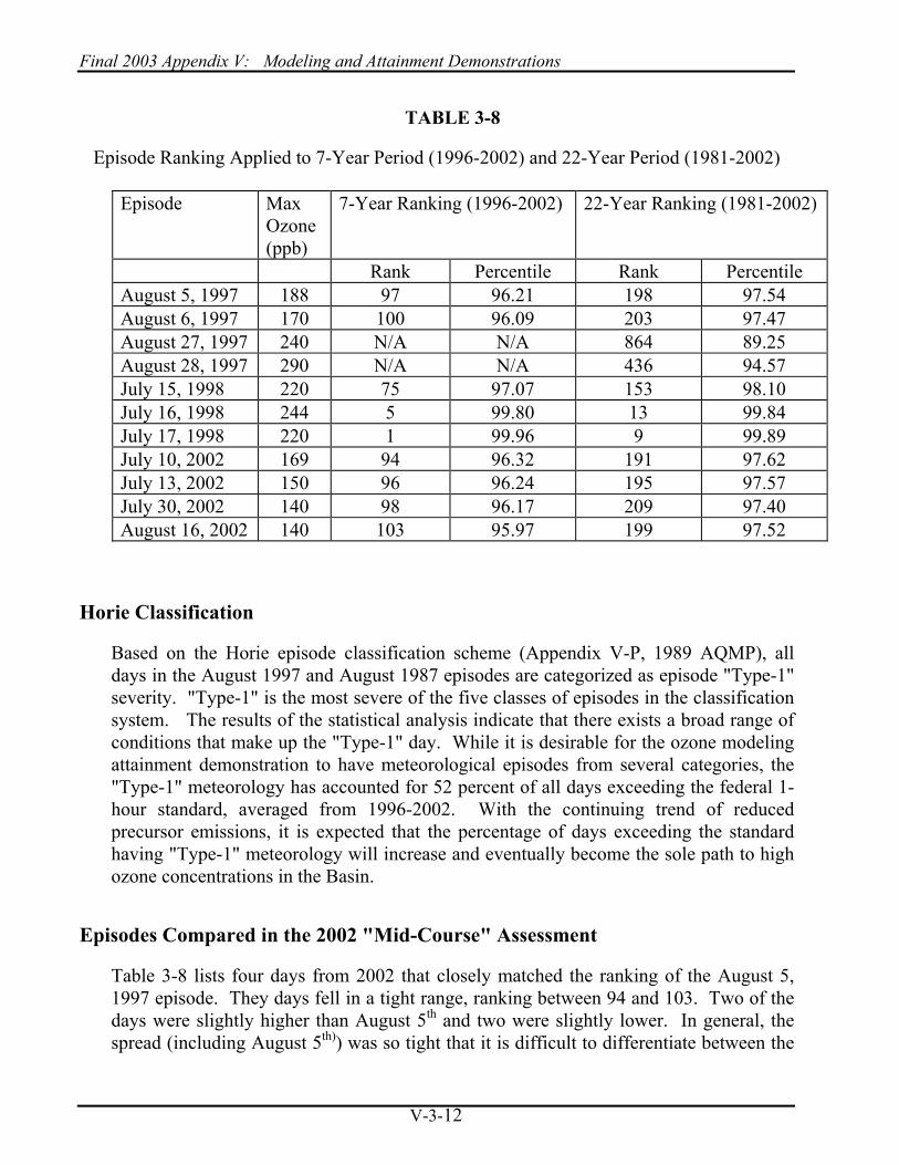
Final 2003 Appendix V: Modeling and Attainment Demonstrations
V-3-12
TABLE 3-8
Episode Ranking Applied to 7-Year Period (1996-2002) and 22-Year Period (1981-2002)
Episode
Max Ozone (ppb)
7-Year Ranking (1996-2002) 22-Year Ranking (1981-2002)
Rank Percentile Rank Percentile August 5, 1997 188 97 96.21 198 97.54 August 6, 1997 170 100 96.09 203 97.47 August 27, 1997 240 N/A N/A 864 89.25 August 28, 1997 290 N/A N/A 436 94.57 July 15, 1998 220 75 97.07 153 98.10 July 16, 1998 244 5 99.80 13 99.84 July 17, 1998 220 1 99.96 9 99.89 July 10, 2002 169 94 96.32 191 97.62 July 13, 2002 150 96 96.24 195 97.57 July 30, 2002 140 98 96.17 209 97.40 August 16, 2002 140 103 95.97 199 97.52
Horie Classification
Based on the Horie episode classification scheme (Appendix V-P, 1989 AQMP), all days in the August 1997 and August 1987 episodes are categorized as episode "Type-1" severity. "Type-1" is the most severe of the five classes of episodes in the classification system. The results of the statistical analysis indicate that there exists a broad range of conditions that make up the "Type-1" day. While it is desirable for the ozone modeling attainment demonstration to have meteorological episodes from several categories, the "Type-1" meteorology has accounted for 52 percent of all days exceeding the federal 1-hour standard, averaged from 1996-2002. With the continuing trend of reduced precursor emissions, it is expected that the percentage of days exceeding the standard having "Type-1" meteorology will increase and eventually become the sole path to high ozone concentrations in the Basin.
Episodes Compared in the 2002 "Mid-Course" Assessment
Table 3-8 lists four days from 2002 that closely matched the ranking of the August 5, 1997 episode. They days fell in a tight range, ranking between 94 and 103. Two of the days were slightly higher than August 5th and two were slightly lower. In general, the spread (including August 5th)) was so tight that it is difficult to differentiate between the

Chapter 3 Revision to the 1997 Ozone Attainment Demonstration Plan
V-3-13
days. The daily maximum ozone concentrations observed on the four days ranged from 140 to 169 ppb with an average of 150 ppb. The average of the observed daily maximum ozone concentrations from the four days that were similar to August 5, 1997 was used by the 2002 "mid-course" assessment to evaluate ozone simulated using 2002 emissions and the August 1997 meteorological episode.
EPISODE CHARACTERIZATION
The meteorological setting characterizing the August 5-6, 1997 episode has been characterized as a part of the SCOS97 monitoring program. The episode has been documented in a special edition of Atmospheric Environment through a special secession of the AWMA Annual Conference, held in San Diego, June 1999. Cassmassi, 1999, and Jackson, et.al. 1999, provide characterization of the general meteorological episode profile used to forecast intensive monitoring, and the data characterizing the structure of the upper air wind and temperature monitoring and the program to profile the vertical ozone structure aloft (through 3000 m).
The following subsections examine the observed synoptic and mesoscale meteorological profiles as well as the ozone air quality that was measured during the August 4-6, 1997 meteorological episode. A detailed discussion of the meteorological and air quality profile observed during the August 27-28, 1987 meteorological episode is presented in Technical Report V-B of the 1994 AQMP.
Background
The August 5-6 1997 meteorological episode resulted in the Basin 2nd highest annual maximum observed ozone concentration 0.188 pbb, measured at Riverside-Rubidoux on August 5th. The characterization of the ozone meteorological episode encompasses five-days (August 3-7, 1997) to bracket the air quality episode. The episode took place during a period of the mid-summer that has one of the greatest frequencies for strong low level inversions, ample sunshine, warm temperatures, and moderate wind transport and ozone episodes.
The meteorological episode began on Sunday August 3 under a ridge of high pressure aloft with 500 mb heights measured by the 1200 UTC San Diego (NKX) sounding in excess of 5900 m each day. Weak onshore flow gave way to stagnant winds through the middle of the episode ultimately resulting in a well developed coastal eddy beginning late on August 6th and continuing into August 7th. Winds observed on August 5th, illustrate a classic “South Route Transport” regime that has been identified as characteristic of past severe Basin ozone meteorological episodes (Keith, 1980).

Final 2003 Appendix V: Modeling and Attainment Demonstrations
V-3-14
Peak inland afternoon temperatures crested over 100 degrees Fahrenheit on each day during the episode and Central Los Angeles consistently reached the mid to upper 90’s. The excessive regional surface temperatures and stagnant flow also contributed to a massive wildfire in the mountainous portions of eastern Ventura and southeastern Santa Barbara counties during the later part of the episode. Using the Horie episodic classification the five days were ranked by the following node categories: August 3rd through August 6th were categorized "Type-1". August 7th was categorized a category "type-1A" (Node 10 on the CART analysis) due to the southerly flow that is consistent with transport north towards Ventura County. The episode types identified by the meteorologists to forecast the intensive monitoring period were consistent with the Horie scheme with the first four days being classified as a South Coast Air Basin maximum or second maximum and August 7th being classified as a transport day to Ventura and Santa Barbara counties.
Synoptic Setting
On the afternoon of August 2nd and throughout August 3rd, a ridge of high pressure aloft developed over the southwest expanding westward from the Four Corners area of the southern Rocky Mountains. Heights at 500 mb reached 5900 m at Vandenberg AFB, San Diego (Miramar NAS) and Desert Rock (Nevada) on August 3rd and remained above that level throughout the five day episode as a weak upper level trough receded into the Pacific Northwest. Figure 3-2 presents the 500 mb pressure height surface for 1200 UTC (0400 PST) on August 5th where a double high pressure system is depicted. All of Southern California is enveloped within the 5940 m contour with an analyzed local 5970 m high located west of the Basin over the Southern California Bight. The August 5th afternoon 850 mb pressure surface (0000 UTC on August 6th) depicted in Figure 3-3 showed temperatures of 28 degrees Celsius and higher over the Basin, indicative of strong subsidence generated by the high-pressure system. Winds along the coast at the 850 mb pressure surface (approximately 1500 m) were generally from the northwest for the bulk of August 5th and 6th. By August 7th, the entire west coast was under the influence of high pressure aloft with only a trace of a short wave trough passing to the north through Washington and British Columbia.
At the surface, high pressure was slowly building in the Great Basin of Nevada pushing a thermal trough westward towards the coast of California. By the morning of August 4th (1200 UTC) the thermal trough had enveloped California with a surface low analyzed near Yuma Arizona running northward to bisect the state (Figure 3.4). This pattern continued until the early morning hours of August 7th as a coast eddy began to develop as the thermal trough moved over the coast. The coast eddy remained in place throughout the day as is evidenced by the presence of reported fog and overcast conditions in the coast plain and as well as the southerly flow.

Chapter 3 Revision to the 1997 Ozone Attainment Demonstration Plan
V-3-15
Mesoscale Meteorology
The mesoscale winds, temperature and pressure gradient fields for the August 3-6th period were generally consistent throughout Southern California. The general profile shifted late on the 6th to the 7th to reflect the development of the coastal eddy. In general, skies were clear throughout the period with the exception of smoke over the Ventura area from the wildfire. All surface pressure gradient fields (along the coast and inland towards the desert) were directed weakly offshore. Under this type of regime, the sea breeze wind flow becomes less organized and often fails to penetrate deep into the Basin – let alone the desert areas. On August 4th, surface winds were predominantly from the west through the coastal plain turning more west-southwesterly on the 5th. By the afternoon of the 6th, southerly flow begins to become evident in the flow field continuing with greater influence on the 7th.
Average afternoon wind speeds ranged between 5 to 10 mph measured at SCAQMD monitoring stations during the period with only a few hours above 10 miles per hour being recorded in the afternoon hours in the eastern SoCAB. Nighttime and morning winds were light and variable on all days during the episode with frequent calms and general speeds recorded at 5 mph or less through 1000 PST.
On August 5th, winds were essentially calm in the morning however the sea breeze came onshore over the central portion of the Basin in response to excessive inland surface heating in Riverside County. The maximum temperature measured on the 5th reached 113 degrees at the Riverside county fire station, 7 degrees warmer than the 4th. The South Route Trajectory typically brings the coastal emissions and brewing smog cloud over southern Los Angeles and Northern Orange counties with transport through the Santa Ana Pass to the eastern portion of the basin. Transport can be noted by a combination of pollution levels, temperature falls and humidity rises in the areas where the sea breeze front traverses. In the areas where the sea breeze has made its incursion an advection inversion with limited mixing becomes established.
The base of the coastal 1200 UTC inversion was at or slightly above the surface throughout the episode. Morning inversion top temperatures ranged from 27.8 to 33.6 degrees C with the peak transcending the morning of the 5th through the morning of the 6th. Despite the strong inversions, the thermal trough over California caused surface temperatures to readily exceed 100 degree Fahrenheit and the inversion was partially broken on the 4th and resulted in deep mixing in the inland valleys on the 5th and 6th. On all three days, the inversion was broken in the San Fernando Valley. Relative humidity values were below 20 percent during the daytime in modest inland areas with only the coastal zone experiencing 40 percent or higher during the earlier periods of the day.
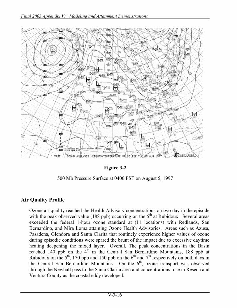
Final 2003 Appendix V: Modeling and Attainment Demonstrations
V-3-16
Figure 3-2
500 Mb Pressure Surface at 0400 PST on August 5, 1997
Air Quality Profile
Ozone air quality reached the Health Advisory concentrations on two day in the episode with the peak observed value (188 ppb) occurring on the 5th at Rubidoux. Several areas exceeded the federal 1-hour ozone standard at (11 locations) with Redlands, San Bernardino, and Mira Loma attaining Ozone Health Advisories. Areas such as Azusa, Pasadena, Glendora and Santa Clarita that routinely experience higher values of ozone during episodic conditions were spared the brunt of the impact due to excessive daytime heating deepening the mixed layer. Overall, The peak concentrations in the Basin reached 140 ppb on the 4th in the Central San Bernardino Mountains, 188 ppb at Rubidoux on the 5th, 170 ppb and 150 ppb on the 6th and 7th respectively on both days in the Central San Bernardino Mountains. On the 6th, ozone transport was observed through the Newhall pass to the Santa Clarita area and concentrations rose in Reseda and Ventura County as the coastal eddy developed.

Chapter 3 Revision to the 1997 Ozone Attainment Demonstration Plan
V-3-17
Figure 3-3
850 Mb Pressure Surface at 1600 PST on August 5, 1997
MODELING METHODOLOGY
The methodology used in modeling ozone is presented next. Since much of the methodology is the same as that used in the 1994 and 1997 AQMP, the reader is referred to Technical Reports V-A and V-B of the 1994 AQMP and Appendix V of the 1997 AQMP for a more complete discussion. Discussion here is limited to the areas in which the procedures used for the 2003 AQMP differ from those used for the 1994 and 1997 AQMPs. First the methods used to develop the inputs are discussed, then the performance of the model is described. This section includes a discussion of some of the uncertainties present in the modeling analysis.

Final 2003 Appendix V: Modeling and Attainment Demonstrations
V-3-18
Figure 3-4
Surface Pressure Contour Analysis at 0400 PST on August 4, 1997
Model Input Preparation
The procedures for UAMAERO-LT input file preparation are presented in this section. Many of the input to the UAM simulations were the same as were used in the previous AQMP ozone modeling attainment demonstrations. The areas of model input preparation that differ from the past practice are discussed at length. In general, the majority of the input files have the same format and structure.
The SCOS97 meteorological data has undergone extensive quality assurance analyses. The meteorological data has been reviewed and flagged where questionable values occur. The Meteorological Working Group of SCOS has reviewed the August 4-6, 1997 meteorological data set at length, comparing wind fields to observational based conceptual models of the episode. The upper air data has undergone additional extensive review by NOAA and STI under contract.

Chapter 3 Revision to the 1997 Ozone Attainment Demonstration Plan
V-3-19
Modeling Domain
The UAM modeling region used to simulate 1-hour average ozone for the 2003 AQMP is presented in Figure 3-1. The area is commonly referred to as the "SCOS97 Modeling Domain" and it covers an area extending from northern Mexico to the southern portion of the San Joaquin Valley. The region extends 550 km in the east-west direction and 370 km in the north-south direction, beginning at the UTM location of 150 easting and 3580 northing. The horizontal extent of the domain used for the UAM analysis is larger than that used for the previous UAM 1997 AQMP simulations or for the current 2003 Draft AQMP UAMAERO-LT PM10 modeling demonstration. Horizontal grid cell resolution was 5 km, as was used in previous UAM modeling applications for the Basin.
The vertical dimensions of the modeling domain are based on previous experience in UAM applications for the Basin and elsewhere. The height of the modeling domain for the UAM simulations was set to a constant 2000 m above ground level. Five spatially and temporally varying layers (based on the mixing height) are used.
Boundary, Top and Initial Air Quality Concentrations
A modified version of the EPA continental average boundary conditions "EPA-Clean" for gaseous pollutants was used as a starting point for the boundary and model-top concentration assignment. Hydrocarbon speciation profiles developed for the 1994 AQMP [Technical Report V-B (1994)] were used to specify the required species. The major adjustment to the "EPA-Clean" profile was to reduce the NO and NO2 concentrations (topcon) to 1.0 and 2.0 part per trillion (ppt). This set of boundary and top concentrations was referred as "ARB-Clean" conditions. The initial condition field was also derived from the monitored air quality data observed for the first day of the simulation. Table 3-9 lists the modified "ARB-Clean" boundary, top concentrations.
A simple vertical pollutant profile was assumed. The boundary cells below the mixing height were given the gridded ground-level pollutant concentrations, and the concentrations in the boundary cells above this level were assumed equal to their corresponding value at the top of the modeling domain.
Future Boundary, Top and Initial Air Quality Conditions
For the future year scenarios, the boundary, region top and ambient air quality concentrations were rolled back based on the percentage reduction in emissions from 1997 base year to the projected emissions levels for future year of the simulation (2002, 2007, or 2010).

Final 2003 Appendix V: Modeling and Attainment Demonstrations
V-3-20
TABLE 3-9
Modified ARB-Clean Boundary and Top Concentrations
Species Units Boundary Top NO PPM 0.000001 0.000001
NO2 PPM 0.002 0.002 O3 PPM 0.04 0.04
OLE PPM 0.000276 0.000276 PAR PPM 0.0137 0.0137 TOL PPM 0.000164 0.000164 XYL PPM 0.00009 0.00009
FORM PPM 0.001928 0.001928 ALD2 PPM 0.000508 0.000508 ETH PPM 0.000468 0.000468
CRES PPM 0.00001 0.00001 OPEN PPM 0.00001 0.00001 PNA PPM 0.00001 0.00001
NXOY PPM 0.00001 0.00001 NO3 PPM 0.00001 0.00001 PAN PPM 0.00001 0.00001 CO PPM 0.2 0.2
HONO PPM 0.000001 0.000001 H2O2 PPM 0.00001 0.00001 HNO3 PPM 0.00001 0.00001 SO2 PPM 0.01 0.01 SO4 PPM 0.0001 0.0001
AERO PPM 3 3
Meteorological Scalars
The METSCALARS file contains information regarding the vertical structure of the modeling region, NO2 photolysis rate constants, and water concentrations. The six parameters in the METSCALARS file are spatially constant values for each time interval described in the file.

Chapter 3 Revision to the 1997 Ozone Attainment Demonstration Plan
V-3-21
• RADFACTOR NO2 photolysis rate constant (min-1) • H2O water concentration (ppm) • ATMOSPRESS atmospheric pressure • CE exposure class • TGRADBELOW temperature gradient below the mixing height • TGRADABOVE temperature gradient above the mixing height
The RADFACTOR (or NO2 photolysis rate constant) inputs for the UAM were prepared using a theoretical solar flux calculation based on clear sky conditions (Schere and Demerjian, 1977).
Water concentration is used in the UAM only for those chemical reactions which contain water as a reactant. The water concentrations were estimated from either dew-point temperatures or relative humidity and surface ambient temperatures which were measured at meteorological monitoring stations and at weather observation stations.
The atmospheric pressure is used in converting molar units (emissions) to concentration units by volume. Since atmospheric pressure does not vary significantly over the SCAB and most of the region is near sea level, a value of one atm was used for all UAM simulations.
The exposure class, which is a numerical representation of the Pasquill stability category, is a function of solar zenith angle and cloud cover. The exposure class was derived from CALMET generated stability class.
Temperature gradients below and above the mixing heights were determined from CALMET generated vertical temperature profile.
Meteorological Models
The CALMET meteorological model was the primary tool used to develop the meteorological fields. CALMET is a terrain following model that is designed primarily to develop three-dimensional wind, temperature and mixing height fields. For this application, CALMET was used to generate the wind and vertical temperature structure. The CALMET mixing heights were evaluated however, the final mixing height fields were generated using a Holzworth (1964) approach (described later). A more comprehensive discussion of the CALMET is provided in the wind field development section.

Final 2003 Appendix V: Modeling and Attainment Demonstrations
V-3-22
Temperature Fields
Surface Analysis
Three-dimensional temperature and humidity fields were developed from the available surface and upper air data using Poisson objective analysis techniques. The SCOS97 data set contained surface station data from approximately 200 reporting stations distributed throughout the modeling domain. The surface stations included data from the ambient air monitoring stations (all APCDs and AQMDs), FAA airport observations, CIMIS, RAWS and offshore buoy sites. In some areas, sites were clustered in close proximity and as a result, the final temperature files were derived from a subset of the total SCOS97 archive. The hourly surface fields were subjected to a 5-point filter to smooth gridded temperature variations.
Figures 3-5 presents the network of surface meteorological stations used in the preparation of the meteorological input fields. Figures 3-6 through 3-11 show the surface temperature fields for 1000 PST and 1600 PST for August 4-6, 1997.
150 250 350 450 550 650UTM Easting
3600
3700
3800
3900
UTM
Nor
thin
g
Figure 3-5
Locations of Surface Monitoring Used in Preparation of Meteorological Fields

Chapter 3 Revision to the 1997 Ozone Attainment Demonstration Plan
V-3-23
Upper Air Analysis
The UAM analysis benefited from the most comprehensive set of upper air data collected in southern California for meteorological episode. Upper air wind and temperature data were continuously measured at 26 Radar Wind Profiler and Radio Acoustic Sounding System (RWP/RASS), at 6 ozone sonde sites, 9 rawinsonde sites and 2 Doppler acoustic sounding sites. Figure 3-12 shows the locations of the upper air monitoring sites. Sounding profiles were assumed to be representative of the upper air structure in the zone for a subjectively determined limited window of time. The temperature data were directly applied to the vertical temperature field interpolation.
The RASS data needed conversion from virtual temperature to sensible temperature. Interpolation of temperature was required to extend the profile from the top of the RASS signal to the top of the modeling domain. Interpolation was also require to extend the temperature profile from the surface to the first range gate where valid data was acquired. The conversion to sensible temperature required the development vertical water vapor profiles for the modeling domain. Water vapor tends to be a conservative element since and as such is a identifying characteristic of an air mass. A single air mass enveloped southern California during the August 1997 episode. As a consequence, the data from the rawinsonde and ozonesondes was sufficient to provide the time and space varying vertical moisture profile needed for the temperature conversion.
Mixing Height Fields
Mixing was calculated using a Holzworth (1964) approach, which estimates the extent of buoyant vertical lifting of an air parcel based on the surface temperature of the air parcel and that of the environment lapse rate measured by the morning and afternoon soundings and the modified RASS temperature profiles.
The hourly mixing heights were calculated, then analyzed and interpolated to a gridded format using a distance-weighted objective analysis. Surface temperature profiles from designated geographical areas were assigned to representative vertical temperature profiles. Hourly objective mixing height calculations mixing within a zone were determined by calculating the interception of the hourly vertical temperature profile and the assumed dry adiabatic ascent of the surface air parcel. If temperature profiles for all 24-hours were not available for a geographical area then linear interpolation of temperature by height level between soundings or modified RASS profiles was used to recreate the vertical structure. The final mixing height fields were smoothes using a 5-point filter. Mixing heights above ground level were restricted to a 2000 m maximum and a 100 m minimum. Figures 3-13 through 3-18 present the mid morning and afternoon mixing heights for the August 4-6, 1997 episode.

Final 2003 Appendix V: Modeling and Attainment Demonstrations
V-3-24
Figure 3-6
Surface Temperature Contours and Observations 1000 PST, August 4, 1997
Figure 3-7
Surface Temperature Contours and Observations 1600 PST, August 4, 1997

Chapter 3 Revision to the 1997 Ozone Attainment Demonstration Plan
V-3-25
Figure 3-8
Surface Temperature Contours and Observations 1000 PST, August 5, 1997
Figure 3-9
Surface Temperature Contours and Observations 1600 PST, August 5, 1997

Final 2003 Appendix V: Modeling and Attainment Demonstrations
V-3-26
Figure 3-10
Surface Temperature Contours and Observations 1000 PST, August 6, 1997
Figure 3-11 Surface Temperature Contours and Observations 1600 PST, August 6, 1997

Chapter 3 Revision to the 1997 Ozone Attainment Demonstration Plan
V-3-27
Figure 3-12
Upper Air Monitoring Network During the August 4-6, 1997 Meteorological Episode
Gridded Wind Fields
The CALMET meteorological model, was used to generate hourly gridded three-dimensional wind fields for the UAM simulations. CALMET is the companion meteorological model to the CALGRID air quality simulation model. CALMET consists of a diagnostic wind field module and micrometeorological module for the boundary layer. CALMET has options to calculate hourly gridded mixing heights and was also used in generating the upper air temperature structure. There are separate boundary layer models for "over land" and "over water" grid cells. For "over land" grid cells, the energy balance method of Holtslag and van Ulden (1983) is used to compute hourly gridded fields of sensible heat flux, surface friction velocity, Monin-Obukhov length, and convective velocity scale. Mixing heights are determined from the computed hourly surface heat fluxes and observed temperature sounding using a modified Carson (1973) method based on Maul (1980). For "over water" grid cells, a profile technique based on air-sea temperature difference is used to compute the micrometeorological parameters in the marine boundary layer. The reader is referred to U.S. EPA et al. (1995) for a complete description of the CALMET meteorological model.

Final 2003 Appendix V: Modeling and Attainment Demonstrations
V-3-28
The diagnostic wind field module uses a two step approach for the computation of the wind fields (Douglas and Kessler, 1990). In the first step, an initial-guess wind field is adjusted for the kinematic effects of terrain, slope flows, and terrain blocking to produce a "Step 1" wind field. The second step consists of an objective analysis procedure to introduce observational data into the "Step 1" wind field to produce a final wind field. An option is provided to allow gridded prognostic wind fields, developed by MM5, to be used by CALMET as the initial guess field. One drawback of inserting the MM5 output is the mismatch in the coordinate systems (UAM/CALMET on a UTM system and MM5 on a Lambert conformal grid). Merging output from the two models requires the data field conversion of either of either meteorology or emissions (which are generated on a UTM coordinate system). With the wealth of observational data available from SCOS97, it was decided to use the objective data to serve as the first guess field.
Wind speed, wind direction, temperature, humidity, cloud cover, ceiling height, and surface pressure were extracted from the SCOS97 extensive RWP, RASS and sodar network, sonde launches and hourly surface observations during the intensive monitoring periods. CALMET employs an inverse-distance-squared or inverse-distance weighted interpolation to transform observed data into gridded fields of the meteorological variables for the specified levels and time. Interpolation is controlled by the maximum radii of influence, number of stations to be used, and barriers. In this analysis barriers were positioned over the ridgelines of the Los Padres, San Gabriel, San Bernardino, San Jacinto and Saddleback mountains.
Land use and land cover (LULC) data files that describe the vegetation, water, natural surface, and cultural feature on the land surface was obtained from the United States Geological Survey. The parameter of soil heat flux was increased from 0.25 to 0.80 for the urban land use. For agricultural, Rangeland and forest, the parameter of soil heat flux was increased to 0.5 from 0.15.
CALMET was run using 16 vertical layers, extending to 5000 m with 11 layers residing in the first 2000 m, three in the lowest 100 m. (Note that UAM domain top was set at 2000 m for the ozone attainment demonstration simulation). UAM layer-averaged winds were created from the CALMET output using a layer matching scheme (UAMWND) developed by Douglas et al. (1990), which weights surface layer wind influence to layers aloft on the basis of stability. For the UAM application, the 3-dimensional winds were converted to a 5-layer format using the UAM layer-matching scheme and the gridded matrix of hourly mixing heights.
.Additional post-processing techniques were selectively applied to the UAM wind fields generated using one or more of the above methodologies. These included the use of a 5-point filter to smooth a UAM wind field to dampen horizontal shear, and use of a filtering technique (which follows a profile suggested by O’Brien [1970]) to adjust UAM vertical velocities and dampen mass flow through the top of the modeling domain.

Chapter 3 Revision to the 1997 Ozone Attainment Demonstration Plan
V-3-29
Figures 3-19 through 3-24 provide the UAM layer-1 winds for 1000 and 1600 PST for August 4-6, 1997. Figures 3-25 through 3-30 provide the UAM layer-3 winds for the same time frame.
Model Input Evaluation
The samples of the meteorological fields that are presented in the preceding sections are discussed in terms of "how well does the meteorology fit the conceptual models"? Given the amount of data acquired during the SCOS97 intensive monitoring program, it was anticipated that the objective analysis should be capable of providing a reasonable recreation of the conceptual model. The following sections address the fit of the model input data to the conceptual model.
Temperature Fields
Briefly, one can assess the August 1997 episode as being very warm on the 4th and 5th with a slight tendency towards cooling the afternoon of the 6th. The temperature fields shown in Figures 3-6 through 3-11 were directly generated from the densely monitored temperature observations. Afternoon temperatures between 35 and 40 oC are captured on the 4th. Temperatures exceeding 40 oC are evident in the inland valleys from the mornings of the 5th through the morning of the 6th indicating the presence of the thermal trough along the coastal zone. Surface temperatures are lower on the afternoon of the 6th as the sea breeze under an eddy circulation pump cooler marine air inland. This pattern fits well with the conceptual model.
Mixing Height Fields
The mixing height fields presented in Figures 3-13 through 3-18 indicated a general pattern of tight mixing gradients across the Basin on the first two days of the episode followed by a weak gradient on the 6th. On the 4th, the eastern and western Basin are separated by the 800 m mixing height contour with the deserts clearly identified by the 1200 to 1500 m contour on the 4th. Mixing on the 5th is deeper with only the coastal zone having mixing less than 1000 m. Both the San Fernando and San Gabriel Valleys have mixing heights exceeding the 1000m level. The desert on this day is essentially indistinguishable for the far eastern Basin with a 1800 m contour acting as an informal breakpoint separating the regions. Mixing on the 6th is typically lower due to the developing eddy and the associated influx of cooler marine modified airflow. The broadly spaced contours show a more uniform level of mixing throughout the Basin, typically below 1000m. The gradient to the desert occurs at about 1600 m contour on this day. The pattern of mixing heights is consistent with the evolution of the episode described by the conceptual model.

Final 2003 Appendix V: Modeling and Attainment Demonstrations
V-3-30
Figure 3-13
Mixing Heights 1000 PST, August 4, 1997
Figure 3-14 Mixing Heights 1600 PST, August 4, 1997

Chapter 3 Revision to the 1997 Ozone Attainment Demonstration Plan
V-3-31
Figure 3-15
Mixing Heights 1000 PST, August 5, 1997
Figure 3-16
Mixing Heights 1600 PST, August 5, 1997

Final 2003 Appendix V: Modeling and Attainment Demonstrations
V-3-32
Figure 3-17
Mixing Heights 1000 PST, August 6, 1997
Figure 3-18
Mixing Heights 1600 PST, August 6, 1997

Chapter 3 Revision to the 1997 Ozone Attainment Demonstration Plan
V-3-33
Figure 3-19
Level-1 UAM Wind Field 1000 PST, August 4, 1997
Figure 3-20
Level-1 UAM Wind Field 1600 PST, August 4, 1997

Final 2003 Appendix V: Modeling and Attainment Demonstrations
V-3-34
Figure 3-21 Level-1 UAM Wind Field 1000 PST, August 5, 1997
Figure 3-22
Level-1 UAM Wind Field 1600 PST, August 5, 1997

Chapter 3 Revision to the 1997 Ozone Attainment Demonstration Plan
V-3-35
Figure 3-23
Level-1 UAM Wind Field 1000 PST, August 6, 1997
Figure 3-24
Level-1 UAM Wind Field 1600 PST, August 6, 1997

Final 2003 Appendix V: Modeling and Attainment Demonstrations
V-3-36
Figure 3-25
Level-3 UAM Wind Fields 1000 PST, August 4 1997
Figure 3-26
Level-3 UAM Wind Fields 1600 PST, August 4, 1997

Chapter 3 Revision to the 1997 Ozone Attainment Demonstration Plan
V-3-37
Figure 3-27
Level-3 UAM Wind Fields 1000 PST, August 5, 1997
Figure 3-28 Level-3 UAM Wind Fields 1600 PST, August 5, 1997

Final 2003 Appendix V: Modeling and Attainment Demonstrations
V-3-38
Figure 3-29
Level-3 UAM Wind Fields 1000 PST, August 6, 1997
Figure 3-30
Level-3 UAM Wind Fields 1600 PST, August 6, 1997
Chapter 3 Revision to the 1997 Ozone Attainment Demonstration Plan
V-3-39
Wind Fields
The winds at UAM levels 1 and 3 are presented to address the flow at the surface and aloft. Figures 3-19 through 3-24 present the 1000 PST and 1600 PST level-1 surface winds. Figures 3-25 through 3-30 present the UAM level-3 winds (first layer above the mixing height).
On the morning of the 4th the surface winds depict a typical onshore flow pattern directed towards the San Gabriel Valley. By 1600, the transport pattern is primarily from west to east with the bulk of transport through the San Gabriel Valley into San Bernardino and northern Riverside Counties. Upper air flow is essential weak in the morning hours and mainly from the northwest. By afternoon, the level-3 winds indicate a westerly sea breeze across the Basin with some continued northwest flow elsewhere.
On the morning of August 5th, surface winds are very light with a poorly organized onshore flow traversing Palos Verdes Peninsula. There is a significant amount of weak along shore flow at the coast. Aloft at level-3, weak drainage flow towards the coast is evident with some north easterly flow inland and across the desert areas. This is consistent with the thermal trough making a move towards the coast and the "desertification" of the Basin is taking place. The drainage aloft with the weak north westerly along shore flow at the surface helped to push the afternoon sea breeze to a southerly transport route though the central Basin and Santa Ana Canyon.
The afternoon winds on the 5th are onshore and westerly with the Elsinore convergence zone depicted in western Riverside County. The flow aloft at level-3 on the afternoon of the 5th was generally out of the northwest. The top of the sea breeze flow over the central Basin and northern Orange County reinforce the surface flow pattern.
By the morning of the 6th southerly wind flow is evident throughout the coastal zone as a eddy is forming in the Santa Monica Bight. The eddy is clearly evident through the southerly flow at level-3 in the morning, weakening somewhat in the afternoon. At the surface (level-1) in the afternoon hours, the flow has taken a north route of transport. Under an eddy flow regime the sea breeze bisects the Basin with one leg of the flow traversing San Fernando Valley and the residual sea breeze causing transport through Cajon Pass and into the San Bernardino Mountains. This pattern is evident in the wind flow depicted by the winds. In general, the wind flow patterns throughout the episode are consistent with the conceptual model.

Final 2003 Appendix V: Modeling and Attainment Demonstrations
V-3-40
1997 BASE-YEAR PERFOMANCE EVALUATION
For the evaluation of the performance of UAM the modeling domain is separated into nine sub-regions or zones. Figure 3-31 depicts the sub-regional zones used for base-year simulation performance. The different zones present unique air quality profiles. In previous ozone modeling attainment demonstrations using a smaller modeling domain, the number and size of the zones was different. Seven zones represented the Basin and portions of Ventura County, the Mojave Desert and the Coachella Valley. As a consequence, a direct overlap of all of the sub-regions does not exist.
For the current analysis the Basin is represented by three of the zones: Zone 3 – the San Fernando Valley, Zone 4 – the Eastern San Gabriel, Riverside and San Bernardino Valleys, and Zone 5 – the Los Angeles and Orange County emissions source areas. Of the four areas, Zone 4 represents the Basin maximum ozone concentrations and the primary downwind impact zone. As such, the priority in evaluating model performance is focus on Zone 4. The 1997 base-year regional model performance for the August 5-6, 1997 and the August 27-28, 1987 episodes in Zones 3, 4, and 5 is presented in Tables 3-10 to 3-12. The ratio of the predicted Basin peak concentration (highest grid level concentration) compared to peak observed concentration is repeated at the top of Tables 3-10 to 3-12 for reference to show the overall capability of the model to simulate maximum concentrations. The regional performance statistics are given in Attachment E. The performance goals for regional ozone are as follows:
Statistic for O3 Criteria (%) Comparison Basis
Normalized Gross Bias ≤ ±15 Paired in space and time Normalized Gross Error ≤ 35 Paired in space (+2 grid
cells) and time Peak Prediction Accuracy ≤ ± 20 Unpaired in space and time
The performance statistics for ozone, and three precursors, nitrogen dioxide, nitric oxide and carbon monoxide are presented in each table. While an increased emphasis has been place on monitoring the different component species of organic compounds through he Photochemical Assessment Monitoring Stations (PAMS) program only a limited number of sites were spread through the modeling domain. As a consequence, meaningful statistics could not be generated for all nine regions. Carbon monoxide is used as a surrogate of the organic compounds for this assessment.
Model performance criteria for nitrogen dioxide are listed in Technical Report VB of the 1994 AQMP. No criteria are available for 1-hour average carbon monoxide or nitric oxide.

Chapter 3 Revision to the 1997 Ozone Attainment Demonstration Plan
V-3-41
Figure 3-31 Performance Evaluation Zones
Statistical Evaluation
The August 1997 UAM ozone simulation met the unpaired peak model performance goal on August 5th in all three zones. The unpaired peak model performance goal is met in zones 3 and 4 on August 6th however zone 5 is over predicted. The gross error was met on the 5th in each zone. The bias tends to be negative -- towards under prediction on the 5th. The bias criterion is met on the 5th in zone 4. In fact, the three performance criteria are met in zone 4 on August 5th. There is a tendency towards over prediction in all zones on the 6th.
The results for the August 1987 ozone simulation show a tendency for under prediction of the peak ozone on in all zones (with the exception of zone 3 on the 28th). The gross error and bias are achieved in each zone on the 28th. While the performance statistics for the August 1987 episode are poorer than for the August 1997 episode, it is important to note that the current AQMP performance for that episode is far better than the base performance for the same episode in the 1997 AQMP. In the 1997 AQMP only after doubling the overall on-road motor vehicle VOC emissions were the ozone performance criteria met.

Final 2003 Appendix V: Modeling and Attainment Demonstrations
V-3-42
TABLE 3-10 Comparative Performance Statistics for Zone 3
Statistic August 1997 August 1987 5th 6th 27th 28th
Ozone Threshold (pphm) 6.0 6.0 8.0 10.0 Ratio of Predicted Basin Peak to Peak Observed
1.05 1.14 0.94 1.08
Ratio of Unpaired Station Peaks
0.80 1.18 0.89 1.26
Systematic Bias (%) -20 6 -2 17 Gross Error (%) 32 44 22 27
NO2 Threshold (pphm) 1.0 1.0 2.0 2.0 Ratio of Unpaired Station Peaks
0.44 0.46 1.25 0.91
Systematic Bias (%) -36 56 11 28 Gross Error (%) 50 59 35 42
NO Threshold (pphm) 1.0 1.0 2.0 2.0 Ratio of Unpaired Station Peaks
1.19 0.53 0.88 0.79
Systematic Bias (%) 43 -61 58 21 Gross Error (%) 110 85 130 85
CO Threshold (pptm)* 2.0 2.0 5.0 5.0 Ratio of Unpaired Station Peaks
0.35 0.54 1.14 1.05
Systematic Bias (%) -62 -47 39 63 Gross Error (%) 62 48 64 80
Bold indicates numbers meeting performance goals.
* Note: No performance criteria for 1-hour average carbon monoxide and nitric oxide were available.

Chapter 3 Revision to the 1997 Ozone Attainment Demonstration Plan
V-3-43
TABLE 3-11 Comparative Performance Statistics for Zone 4
Statistic August 1997 August 1987 5th 6th 27th 28th
Ozone Threshold (pphm) 6.0 6.0 8.0 10.0 Ratio of Predicted Basin Peak to Peak Observed
1.05 1.14 0.94 1.08
Ratio of Unpaired Station Peaks
1.01 1.10 0.83 0.79
Systematic Bias (%) -4 18 -23 -1 Gross Error (%) 25 40 34 21
NO2 Threshold (pphm) 1.0 1.0 2.0 2.0 Ratio of Unpaired Station Peaks
0.53 0.62 0.97 0.95
Systematic Bias (%) -40 -56 14 40 Gross Error (%) 51 58 57 68 NO Threshold (pphm) 1.0 1.0 2.0 2.0 Ratio of Unpaired Station Peaks
1.10 0.44 1.16 1.19
Systematic Bias (%) -31 -60 -26 -16 Gross Error (%) 90 81 61 61
CO Threshold (pptm)* 2.0 2.0 5.0 5.0 Ratio of Unpaired Station Peaks
0.58 0.36 1.11 0.97
Systematic Bias (%) -45 -48 7 38 Gross Error (%) 50 48 52 64
Bold indicates numbers meeting performance goals.
* Note: No performance criteria for 1-hour average carbon monoxide and nitric oxide were available.

Final 2003 Appendix V: Modeling and Attainment Demonstrations
V-3-44
TABLE 3-12 Comparative Performance Statistics for Zone 5
Statistic August 1997 August 1987 5th 6th 27th 28th
Ozone Threshold (pphm) 6.0 6.0 8.0 10.0 Ratio of Predicted Basin Peak to Peak Observed
1.05 1.14 0.94 1.08
Ratio of Unpaired Station Peaks
1.11 1.24 0.85 0.91
Systematic Bias (%) -23 -43 -19 -4 Gross Error (%) 32 62 21 19
NO2 Threshold (pphm) 1.0 1.0 2.0 2.0 Ratio of Unpaired Station Peaks
0.60 0.82 1.14 1.70
Systematic Bias (%) 16 12 57 113 Gross Error (%) 44 43 62 115
NO Threshold (pphm) 1.0 1.0 2.0 2.0 Ratio of Unpaired Station Peaks
1.85 0.83 1.90 2.21
Systematic Bias (%) 122 -1 70 73 Gross Error (%) 162 103 105 114
CO Threshold (pptm) 2.0 2.0 5.0 5.0 Ratio of Unpaired Station Peaks
1.13 1.50 1.39 2.26
Systematic Bias (%) 37 -20 70 94 Gross Error (%) 62 61 80 102
Bold indicates numbers meeting performance goals.
* Note: No performance criteria for 1-hour average carbon monoxide and nitric oxide were available.
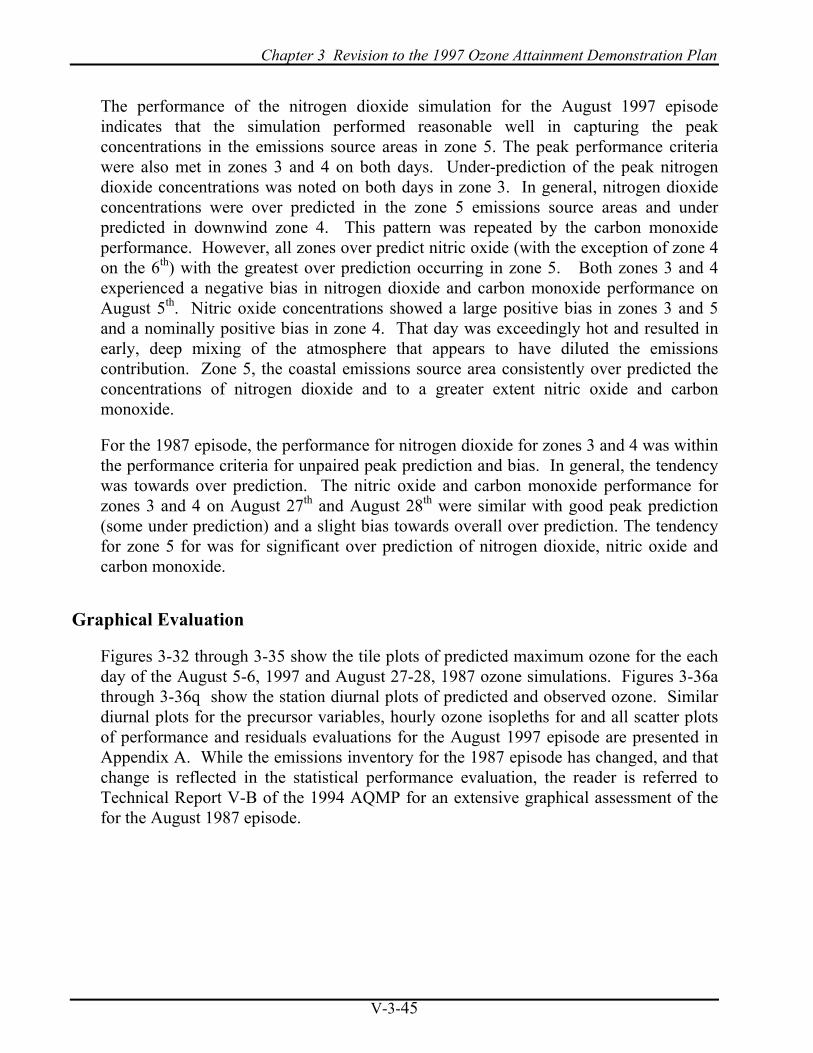
Chapter 3 Revision to the 1997 Ozone Attainment Demonstration Plan
V-3-45
The performance of the nitrogen dioxide simulation for the August 1997 episode indicates that the simulation performed reasonable well in capturing the peak concentrations in the emissions source areas in zone 5. The peak performance criteria were also met in zones 3 and 4 on both days. Under-prediction of the peak nitrogen dioxide concentrations was noted on both days in zone 3. In general, nitrogen dioxide concentrations were over predicted in the zone 5 emissions source areas and under predicted in downwind zone 4. This pattern was repeated by the carbon monoxide performance. However, all zones over predict nitric oxide (with the exception of zone 4 on the 6th) with the greatest over prediction occurring in zone 5. Both zones 3 and 4 experienced a negative bias in nitrogen dioxide and carbon monoxide performance on August 5th. Nitric oxide concentrations showed a large positive bias in zones 3 and 5 and a nominally positive bias in zone 4. That day was exceedingly hot and resulted in early, deep mixing of the atmosphere that appears to have diluted the emissions contribution. Zone 5, the coastal emissions source area consistently over predicted the concentrations of nitrogen dioxide and to a greater extent nitric oxide and carbon monoxide.
For the 1987 episode, the performance for nitrogen dioxide for zones 3 and 4 was within the performance criteria for unpaired peak prediction and bias. In general, the tendency was towards over prediction. The nitric oxide and carbon monoxide performance for zones 3 and 4 on August 27th and August 28th were similar with good peak prediction (some under prediction) and a slight bias towards overall over prediction. The tendency for zone 5 for was for significant over prediction of nitrogen dioxide, nitric oxide and carbon monoxide.
Graphical Evaluation
Figures 3-32 through 3-35 show the tile plots of predicted maximum ozone for the each day of the August 5-6, 1997 and August 27-28, 1987 ozone simulations. Figures 3-36a through 3-36q show the station diurnal plots of predicted and observed ozone. Similar diurnal plots for the precursor variables, hourly ozone isopleths for and all scatter plots of performance and residuals evaluations for the August 1997 episode are presented in Appendix A. While the emissions inventory for the 1987 episode has changed, and that change is reflected in the statistical performance evaluation, the reader is referred to Technical Report V-B of the 1994 AQMP for an extensive graphical assessment of the for the August 1987 episode.

Final 2003 Appendix V: Modeling and Attainment Demonstrations
V-3-46
Figure 3-32
UAM Simulated Maximum 1-Hour Average Ozone, August 5, 1997
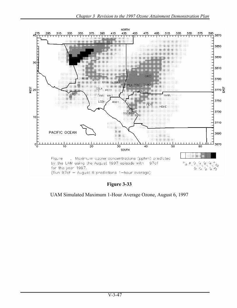
Chapter 3 Revision to the 1997 Ozone Attainment Demonstration Plan
V-3-47
Figure 3-33
UAM Simulated Maximum 1-Hour Average Ozone, August 6, 1997
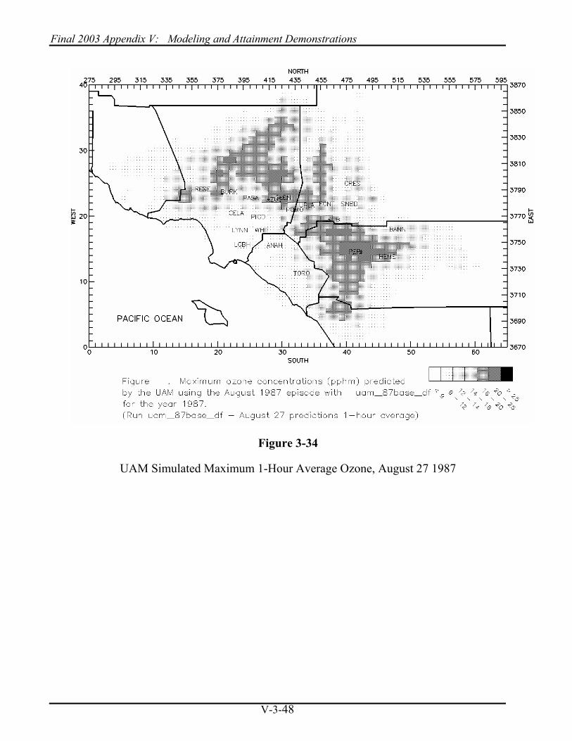
Final 2003 Appendix V: Modeling and Attainment Demonstrations
V-3-48
Figure 3-34
UAM Simulated Maximum 1-Hour Average Ozone, August 27 1987

Chapter 3 Revision to the 1997 Ozone Attainment Demonstration Plan
V-3-49
Figure 3-35
UAM Simulated Maximum 1-Hour Average Ozone, August 28, 1987

Final 2003 Appendix V: Modeling and Attainment Demonstrations
V-3-50
Figure 3-36a
UAM Simulated Maximum 1-Hour Average Ozone (Solid Line) Vs. Observed (Squares):
August 3-7, 1997 Ozone Meteorological Episode

Chapter 3 Revision to the 1997 Ozone Attainment Demonstration Plan
V-3-51
Figure 3-36b
UAM Simulated Maximum 1-Hour Average Ozone (Solid Line) Vs. Observed (Squares):
August 3-7, 1997 Ozone Meteorological Episode

Final 2003 Appendix V: Modeling and Attainment Demonstrations
V-3-52
Figure 3-36c
UAM Simulated Maximum 1-Hour Average Ozone (Solid Line) Vs. Observed (Squares):
August 3-7, 1997 Ozone Meteorological Episode

Chapter 3 Revision to the 1997 Ozone Attainment Demonstration Plan
V-3-53
Figure 3-36d
UAM Simulated Maximum 1-Hour Average Ozone (Solid Line) Vs. Observed (Squares):
August 3-7, 1997 Ozone Meteorological Episode

Final 2003 Appendix V: Modeling and Attainment Demonstrations
V-3-54
Figure 3-36e
UAM Simulated Maximum 1-Hour Average Ozone (Solid Line) Vs. Observed (Squares):
August 3-7, 1997 Ozone Meteorological Episode

Chapter 3 Revision to the 1997 Ozone Attainment Demonstration Plan
V-3-55
Figure 3-36f
UAM Simulated Maximum 1-Hour Average Ozone (Solid Line) Vs. Observed (Squares):
August 3-7, 1997 Ozone Meteorological Episode

Final 2003 Appendix V: Modeling and Attainment Demonstrations
V-3-56
Figure 3-36g
UAM Simulated Maximum 1-Hour Average Ozone (Solid Line) Vs. Observed (Squares):
August 3-7, 1997 Ozone Meteorological Episode

Chapter 3 Revision to the 1997 Ozone Attainment Demonstration Plan
V-3-57
Figure 3-36h
UAM Simulated Maximum 1-Hour Average Ozone (Solid Line) Vs. Observed (Squares):
August 3-7, 1997 Ozone Meteorological Episode

Final 2003 Appendix V: Modeling and Attainment Demonstrations
V-3-58
Figure 3-36i
UAM Simulated Maximum 1-Hour Average Ozone (Solid Line) Vs. Observed (Squares):
August 3-7, 1997 Ozone Meteorological Episode

Chapter 3 Revision to the 1997 Ozone Attainment Demonstration Plan
V-3-59
Figure 3-36j
UAM Simulated Maximum 1-Hour Average Ozone (Solid Line) Vs. Observed (Squares):
August 3-7, 1997 Ozone Meteorological Episode

Final 2003 Appendix V: Modeling and Attainment Demonstrations
V-3-60
Figure 3-36k
UAM Simulated Maximum 1-Hour Average Ozone (Solid Line) Vs. Observed (Squares):
August 3-7, 1997 Ozone Meteorological Episode

Chapter 3 Revision to the 1997 Ozone Attainment Demonstration Plan
V-3-61
Figure 3-36l
UAM Simulated Maximum 1-Hour Average Ozone (Solid Line) Vs. Observed (Squares):
August 3-7, 1997 Ozone Meteorological Episode

Final 2003 Appendix V: Modeling and Attainment Demonstrations
V-3-62
Figure 3-36m
UAM Simulated Maximum 1-Hour Average Ozone (Solid Line) Vs. Observed (Squares):
August 3-7, 1997 Ozone Meteorological Episode

Chapter 3 Revision to the 1997 Ozone Attainment Demonstration Plan
V-3-63
Figure 3-36n
UAM Simulated Maximum 1-Hour Average Ozone (Solid Line) Vs. Observed (Squares):
August 3-7, 1997 Ozone Meteorological Episode

Final 2003 Appendix V: Modeling and Attainment Demonstrations
V-3-64
Figure 3-36o
UAM Simulated Maximum 1-Hour Average Ozone (Solid Line) Vs. Observed (Squares):
August 3-7, 1997 Ozone Meteorological Episode

Chapter 3 Revision to the 1997 Ozone Attainment Demonstration Plan
V-3-65
Figure 3-36p
UAM Simulated Maximum 1-Hour Average Ozone (Solid Line) Vs. Observed (Squares):
August 3-7, 1997 Ozone Meteorological Episode

Final 2003 Appendix V: Modeling and Attainment Demonstrations
V-3-66
Figure 3-36q
UAM Simulated Maximum 1-Hour Average Ozone (Solid Line) Vs. Observed (Squares):
August 3-7, 1997 Ozone Meteorological Episode

Chapter 3 Revision to the 1997 Ozone Attainment Demonstration Plan
V-3-67
On August 5th, the peaks are nominally under predicted and tend to lag the observed concentrations in the San Fernando Valley and West L.A. areas. The simulation tends to under predicted observations in the San Gabriel Valley but and has a mixed scorecard for the coastal-metropolitan areas fitting the observed pattern from Long Beach to Anaheim with a slight lag in timing at La Habra and El Toro. In general, the eastern Basin stations have a better fit of the observed distribution with Rubidoux being slightly under predicted and Elsinore and Temecula being over predicted with a lag in the maximum prediction. The tile plot (Figure 3-32) shows a maximum impact occurring in southwestern Riverside and the northern tip of San Diego County. The displacement in the maximum predicted concentration may reflect the impact of biogenic emissions in the Santa Ana Mountains. Another possible reason may be a subtle shift in the onshore flow that may have pushed the pollutant cloud too far south, missing the traverse through the Santa Ana Canyon. Regardless, peak concentrations in the primary impact zone of Riverside and San Bernardino Counties are well represented.
On the 6th, concentrations of ozone are over predicted in the coastal and near valley portions of Ventura county in response to the eddy circulation. The tile plot (Figure 3-33) shows a hot spot in the northeastern portion of Ventura County relating to a brush fire that erupted during the episode. Very little ozone was generated in the coast-metropolitan areas. The inland valleys generated the appropriate maximum concentrations but the timing lagged observations. What show in the tile plot is the split in the impact zone in response to the bifurcation of the surface wind trajectories under the eddy circulation.
Briefly, the tile plots for August 27 and August 28, 1987 (Figures 3-34 and 3-35) depict primary ozone impacts in the eastern San Gabriel Valley and east Basin (predicted and observed concentration exceeding .020 ppm) and secondary impact to the San Fernando Valley. The level of the predicted impact is consistent with observations
Effect of Emissions Uncertainties
Great effort was undertaken in the SCOS97 program and the ensuing updates to the mobile and day specific point and biogenic inventories to remedy may of the problems identified in prior AQMP modeling attainment demonstrations. Aircraft and airport operations were thoroughly reviewed and inventoried. Shipping transits into the Ports of Los Angeles and Long Beach were carefully logged and shipping lane transits up and down the coast were logged for the major vessels. The biogenic emissions inventory under went significant modification and resulted in several peer review papers outlining the inventory process. A whole revamp of the emissions surrogates used to distribute areas source emissions was conducted as well.

Final 2003 Appendix V: Modeling and Attainment Demonstrations
V-3-68
Of the inventory upgrades, none had as much impact as the revisions to ARB's on-road emissions program EMFAC2002 and the development of an Off-Road companion model. The net impact of EMFAC2002 was to raise the absolute tonnage of NOx and VOC in the mobile source emissions inventory. For example, the Basin totals for VOC and NOx for the August 28, 1987 episode increased from 1969 and 1379 tons TPD in the 1997 AQMP to 2446 and 1846 TPD for the current effort. While VOC emissions rose 24 percent NOx emissions rose by a greater 34 percent margin. Many of the complaints of the episode development in the 1994 and 1997 episode was that there existed too much NOx relative to the amount of VOC in the domain. The upgrade to the inventories may have corrected several of the faults in the previous analyses but the ratio of VOC to NOx remained in favor of ozone titration in the coastal emissions region.
The higher relative amounts of NOx in the inventory may be a cause for the bias towards over prediction of NOx in Zone 5 and may have affected the model performance not only for UAM but for CALGRID and CAMx. UAM deposition terms will remove NOx at a fast rate relative to the response of several of the other air quality simulation models evaluated including CALGRID and CAMx. (This was confirmed by the preliminary performance evaluations of CALGRID and CAMx which are not presented in this discussion). Overall, the net amount of NOx deposition deposited by the UAM is greatest with CALGRID coming in second place. The CAMx net NOx deposition was substantially lower. The impact of grater deposition may have lead to higher downwind ozone formation (possible as high as 10 ppb) and alterations in the timing of the formation.
Several additional factors resulting from the use of the EMFAC2002 and Direct Transportation Impact Model (DTIM4) to generate grid level mobile source emissions may have altered the VOC to NOx ratio in the Basin. First, there exist differences between the two models in the numbers of trips and lengths of trips inferred by the regional transportation model output. More numerous starts and stops lead to greater VOC emissions from vehicle use and standing evaporative loss. Similarly, speed impacts the NOx emissions, especially from heavy duty diesels. Differences between the emissions models in how the truck speed factors are assigned may have lead to an overestimation of NOx. These aspects of the emissions inventory generation were identified in the development process and some corrections to the evaporative loss calculations were made. In addition a sensitivity simulation was run with increased VOC and lower NOx that would be expected to occur if truck speeds were reduced. The net impact also raised the predicted amount of ozone formed in the Basin.
Other areas of the inventory uncertainty may have impacted the UAM (and other models) performance including the assignment of surrogates used to distribute emissions through the Basin, and the sub-county distribution of vehicles by age. Several sensitivity simulations were conducted using emissions factors generated by EMFAC2002 using a grid level characterization of the passenger vehicle age with each

Chapter 3 Revision to the 1997 Ozone Attainment Demonstration Plan
V-3-69
county. The analysis was designed to attempt to place older, high emitting vehicles in the general areas where they operate. There are drawbacks to this assumption in that the average trip distance in the Basin exceeds one grid length and can easily transverse a county line. The sensitivity analyses are ongoing and preliminary results suggest some changes in the ozone simulation model performance. However, the net impact would be minor, less than the 10 ppb identified by deposition terms.
The biogenic inventory is also subject to uncertainties due to the critical roll daily temperature and humidity has in the estimation of the emissions. This is clearly evident in the day-to-day variation in total emissions over the three day 1997 episode, and in the difference in the estimated emissions between 1987 and 1997. Also the speciation profile of the hydrocarbons emanating from the biogenic mass is a source of uncertainty, particularly for the SAPRC99 chemistry. Finally, the episodes take place in August and it is difficult to assess cumulative stress on the biomass over the season and what impact did the stress have on daily emissions.
While the uncertainties exist in this analysis, the overall baseline performance of UAM is significantly better than the unadjusted UAM performance presented in the 1994 and 1997 ozone attainment demonstration plans. Additional stress tests on the August 1997 ozone meteorological episode are presented later in this chapter.
MID-COURSE OZONE AIR QUALITY EVALUATION
As discussed in Chapter 1 and earlier in this chapter, a "mid-course" evaluation of UAM performance was conducted using the 2002 projected baseline emissions inventory and the August 1997 meteorological episodes. The "mid-course" evaluation is a weight of evidence tool that is used to demonstrate that the model simulation is responding to changes in the emissions trend. The ability of the model to simulate ozone concentrations for days having a similar meteorological profile to those included in the meteorological episode for an independent set of emissions is a powerful statement that the simulations is reasonable and that the emissions trend is on the correct track. A one-to-one correspondence is not expected since the days in 2002 are not exact duplicates of the 1997 and 1987 episode days.
For this mid-course analysis, four days were identified in 2002 that ranked within ± 6 of the August 5, 1997 based on the 7-year ranking algorithm. The average observed ozone concentration for the four days (two ranked above and two ranked below) was 150 ppb. The process was repeated for August 6th using the 7-year ranking with the caveat of selecting the two days most closely ranked above and below the episode day ranking. For the 1987 episode, the process was repeated but the 22-year ranking was used as a classification. The tightest grouping of days ranked in 2002 that were similar to those in either episode occurred for August 5, 1997 and August 6, 1997.

Final 2003 Appendix V: Modeling and Attainment Demonstrations
V-3-70
The simulation was conducted using the 2002 baseline emissions (grown from 1997) and adjusted boundary conditions. Table 3-13 summarizes the simulation and Figures 3-37 through 3-40 depict the tile plots of predicted 1-hour maximum ozone. In general, the peak values of tend to be slightly over predicted for the 2002 4-day average observed daily maximum ozone concentrations. Only one of the four simulated Basin maximum days falls within the range of observations on the four days in 2002 that comprise the corresponding average day. However, the peak predicted ozone concentration (170 ppb for the August 5, 1997 episode) is comparable with the observed 2002 annual Basin maximum concentration of 169 ppb.
Little change in the spatial distribution of predicted Basin maximum ozone is depicted in the tile plots suggesting no radical changes have taken place in the relative contributions of VOC, NOx and carbon monoxide emissions since the base year.
TABLE 3-13 2002 Mid-Course Simulation Results
Episode Day UAM Predicted (ppb)
4-Day 2002 Historical Average
Ozone (ppb)
Range of Observations for
Comparable days in 2002 (ppb)
August 5, 1997 170 150 140 - 169 August 6, 1997 168 140 130 - 150 August 27, 1987 126 123 100 - 140 August 28, 1987 149 115 110 - 120

Chapter 3 Revision to the 1997 Ozone Attainment Demonstration Plan
V-3-71
Figure 3-37
2002 UAM Simulated Maximum 1-Hour Average Ozone for the
August 5, 1997 Ozone Meteorological Episode

Final 2003 Appendix V: Modeling and Attainment Demonstrations
V-3-72
Figure 3-38
2002 UAM Simulated Maximum 1-Hour Average Ozone for the
August 6, 1997 Ozone Meteorological Episode

Chapter 3 Revision to the 1997 Ozone Attainment Demonstration Plan
V-3-73
Figure 3-39
2002 UAM Simulated Maximum 1-Hour Average Ozone for the
August 27, 1987 Ozone Meteorological Episode

Final 2003 Appendix V: Modeling and Attainment Demonstrations
V-3-74
Figure 3-40
2002 UAM Simulated Maximum 1-Hour Average Ozone for the
August 28, 1987 Ozone Meteorological Episode

Chapter 3 Revision to the 1997 Ozone Attainment Demonstration Plan
V-3-75
OZONE AIR QUALITY PROJECTIONS
UAM simulations were conducted for the future year base emission scenarios (2007, 2010 and 2020), and future year controlled scenarios (2007, 2010 [two-options], and 2020). Historical year modeling and model performance evaluation are discussed earlier. The impact of base and controlled emissions on ozone air quality is projected for all modeling episodes for the years 2007 2010 and 2020. The baseline and controlled emission projections for the historical and future years are given in Tables 3-2, 3-4 and 3-5.
Projection of 2007 Air Quality
One major component of the 2003 AQMP modeling attainment demonstration addresses the issue of transport of ozone and precursor pollutants into the Coachella Valley, Antelope Valley, South Central Coastal Air Basin and Mojave Desert. The attainment year for each of these areas is 2007.
Focused UAM-predicted Coachella Valley maximum ozone concentration maps for the year 2007 are presented in Figures 3-41 through 3-44 for each day of the two modeling episodes. For the 2007 projection, the controlled emissions scenario is presented. Emission reductions through 2007 are expected to take place through exiting established control measures and reductions in mobile source emissions as projected by EMFAC2002. By 2007, all areas of the Coachella Valley demonstrate attainment of the federal ozone standard. Table 3-14 lists the 2007 predicted air quality for the Coachella Valley, the Basin, and its neighboring transport partners.
The projected 2007 air quality for all non-Basin areas indicates that ozone is expected to meet the federal standard. UAM simulations for three of the episode days modeled indicated that predicted ozone concentrations will be below the 124 ppb. The UAM simulation for the August 6th episode indicated that a limited number of grid cells adjacent to the Basin, north of Cajon Pass transecting both Antelope Valley and the Mojave Desert, would exceed 124 ppb. (A 148 ppb maximum predicted grid cell ozone concentration was project for the Mojave Desert). However, the August 6th base-year UAM simulation over predicted ozone concentrations at neighboring stations Hesperia and Victorville by an average of 33 percent and Lancaster in the Antelope Valley by 71 percent. (CALGRID, which under predicted the base-year Basin maximum by 12 percent, also over predicted in this portion of the high desert by 9 percent for the same day). By adjusting the 2007 UAM simulation in the local areas for the base-year over prediction, the estimated Mojave Desert impact is lowered to 111 ppb and the Antelope Valley impact to 99 ppb. This correction is consistent with the projected is consistent with the direct UAM simulation for the remaining three episode days.

Final 2003 Appendix V: Modeling and Attainment Demonstrations
V-3-76
TABLE 3-14 UAM Simulated 2007 Maximum Ozone: Controlled Emissions
Episode Day Basin
Coachella Valley
Antelope Valley
Mojave Desert
Ventura- South
Central Coast
August 5, 1997 145 122 92 118 89 August 6, 1997 151 83 141 (99)* 148 (111)* 106 August 27, 1987 115 94 99 115 101 August 28, 1987 138 83 105 119 103
* Concentration for the high desert inside the brackets is the scaled value to adjust for
systematic over prediction in the base year
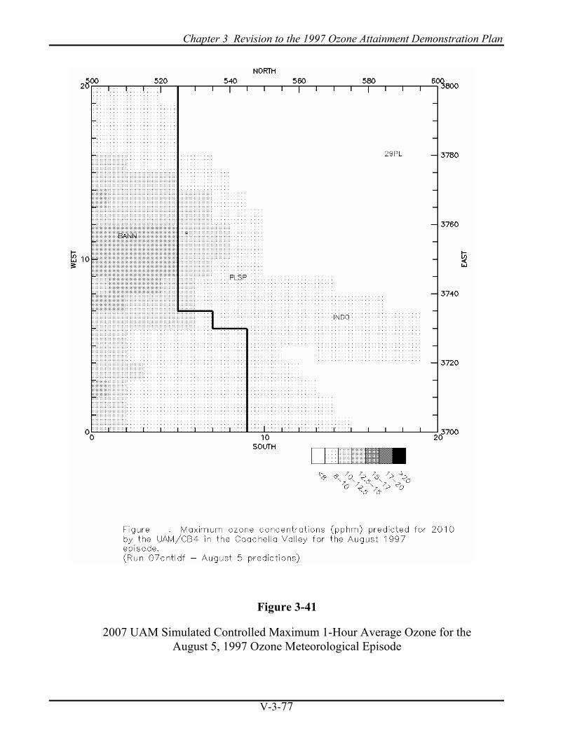
Chapter 3 Revision to the 1997 Ozone Attainment Demonstration Plan
V-3-77
Figure 3-41
2007 UAM Simulated Controlled Maximum 1-Hour Average Ozone for the August 5, 1997 Ozone Meteorological Episode

Final 2003 Appendix V: Modeling and Attainment Demonstrations
V-3-78
Figure 3-42
2007 UAM Simulated Controlled Maximum 1-Hour Average Ozone for the August 6, 1997 Ozone Meteorological Episode
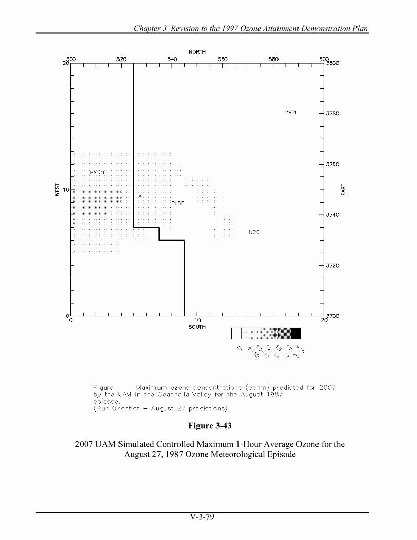
Chapter 3 Revision to the 1997 Ozone Attainment Demonstration Plan
V-3-79
Figure 3-43
2007 UAM Simulated Controlled Maximum 1-Hour Average Ozone for the August 27, 1987 Ozone Meteorological Episode

Final 2003 Appendix V: Modeling and Attainment Demonstrations
V-3-80
Figure 3-44
2007 UAM Simulated Controlled Maximum 1-Hour Average Ozone for the August 28, 1987 Ozone Meteorological Episode
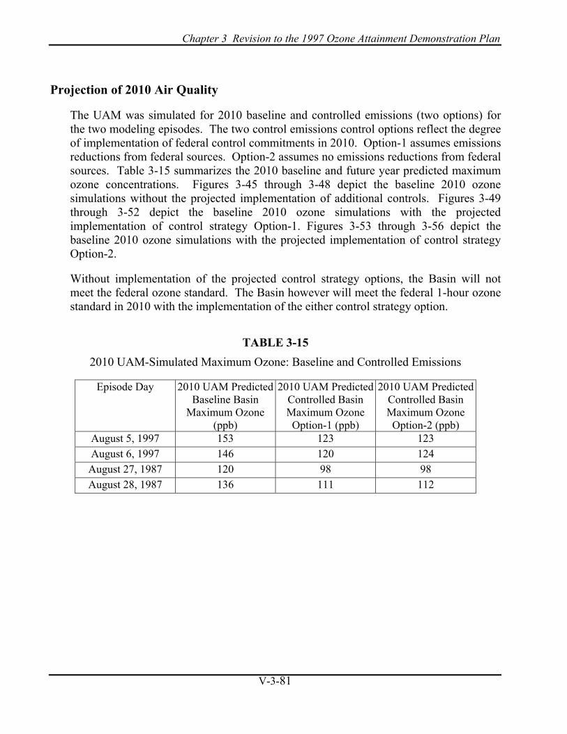
Chapter 3 Revision to the 1997 Ozone Attainment Demonstration Plan
V-3-81
Projection of 2010 Air Quality
The UAM was simulated for 2010 baseline and controlled emissions (two options) for the two modeling episodes. The two control emissions control options reflect the degree of implementation of federal control commitments in 2010. Option-1 assumes emissions reductions from federal sources. Option-2 assumes no emissions reductions from federal sources. Table 3-15 summarizes the 2010 baseline and future year predicted maximum ozone concentrations. Figures 3-45 through 3-48 depict the baseline 2010 ozone simulations without the projected implementation of additional controls. Figures 3-49 through 3-52 depict the baseline 2010 ozone simulations with the projected implementation of control strategy Option-1. Figures 3-53 through 3-56 depict the baseline 2010 ozone simulations with the projected implementation of control strategy Option-2.
Without implementation of the projected control strategy options, the Basin will not meet the federal ozone standard. The Basin however will meet the federal 1-hour ozone standard in 2010 with the implementation of the either control strategy option.
TABLE 3-15 2010 UAM-Simulated Maximum Ozone: Baseline and Controlled Emissions
Episode Day 2010 UAM Predicted Baseline Basin
Maximum Ozone (ppb)
2010 UAM Predicted Controlled Basin Maximum Ozone Option-1 (ppb)
2010 UAM Predicted Controlled Basin Maximum Ozone Option-2 (ppb)
August 5, 1997 153 123 123 August 6, 1997 146 120 124 August 27, 1987 120 98 98 August 28, 1987 136 111 112

Final 2003 Appendix V: Modeling and Attainment Demonstrations
__________________________________________________________________________V-3-82
Figure 3-45
2010 UAM Simulated Baseline Maximum 1-Hour Average Ozone for the August 5, 1997 Ozone Meteorological Episode

Chapter 3 Revision to the 1997 Ozone Attainment Demonstration Plan
V-3-83
Figure 3-46
2010 UAM Simulated Baseline Maximum 1-Hour Average Ozone for the August 6, 1997 Ozone Meteorological Episode

Final 2003 Appendix V: Modeling and Attainment Demonstrations
__________________________________________________________________________V-3-84
Figure 3-47
2010 UAM Simulated Baseline Maximum 1-Hour Average Ozone for the August 27, 1987 Ozone Meteorological Episode

Chapter 3 Revision to the 1997 Ozone Attainment Demonstration Plan
V-3-85
Figure 3-48
2010 UAM Simulated Baseline Maximum 1-Hour Average Ozone for the August 28, 1987 Ozone Meteorological Episode

Final 2003 Appendix V: Modeling and Attainment Demonstrations
__________________________________________________________________________V-3-86
Figure 3-49
2010 UAM Simulated Controlled Maximum 1-Hour Average Ozone for the August 5, 1997 Ozone Meteorological Episode--Option-1

Chapter 3 Revision to the 1997 Ozone Attainment Demonstration Plan
V-3-87
Figure 3-50
2010 UAM Simulated Controlled Maximum 1-Hour Average Ozone for the August 6, 1997 Ozone Meteorological Episode--Option-1

Final 2003 Appendix V: Modeling and Attainment Demonstrations
__________________________________________________________________________V-3-88
Figure 3-51
2010 UAM Simulated Controlled Maximum 1-Hour Average Ozone for the August 27, 1987 Ozone Meteorological Episode--Option-1

Chapter 3 Revision to the 1997 Ozone Attainment Demonstration Plan
V-3-89
Figure 3-52
2010 UAM Simulated Controlled Maximum 1-Hour Average Ozone for the August 28, 1987 Ozone Meteorological Episode--Option-1
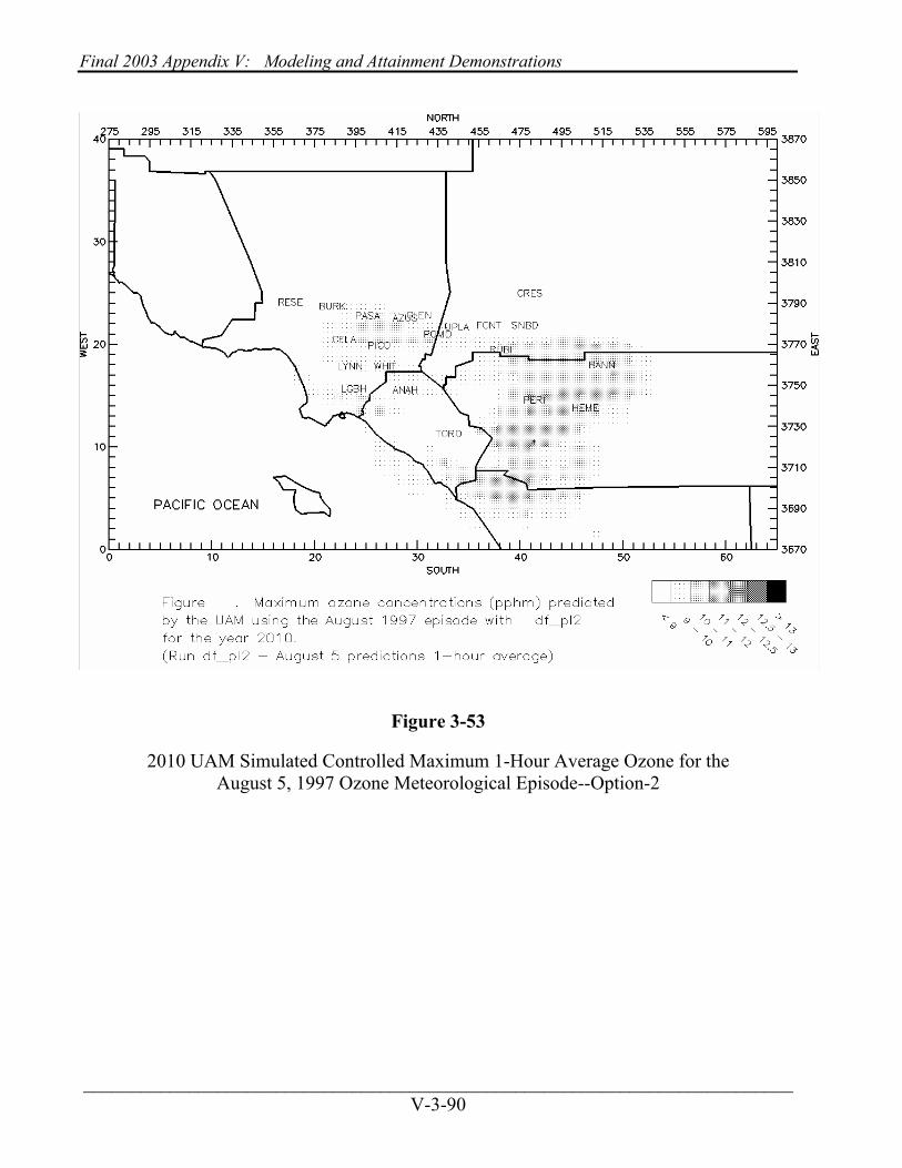
Final 2003 Appendix V: Modeling and Attainment Demonstrations
__________________________________________________________________________V-3-90
Figure 3-53
2010 UAM Simulated Controlled Maximum 1-Hour Average Ozone for the August 5, 1997 Ozone Meteorological Episode--Option-2

Chapter 3 Revision to the 1997 Ozone Attainment Demonstration Plan
V-3-91
Figure 3-54
2010 UAM Simulated Controlled Maximum 1-Hour Average Ozone for the August 6, 1997 Ozone Meteorological Episode--Option-2

Final 2003 Appendix V: Modeling and Attainment Demonstrations
__________________________________________________________________________V-3-92
Figure 3-55
2010 UAM Simulated Controlled Maximum 1-Hour Average Ozone for the August 27, 1987 Ozone Meteorological Episode--Option-2

Chapter 3 Revision to the 1997 Ozone Attainment Demonstration Plan
V-3-93
Figure 3-56
2010 UAM Simulated Controlled Maximum 1-Hour Average Ozone for the August 28, 1987 Ozone Meteorological Episode--Option-2

Final 2003 Appendix V: Modeling and Attainment Demonstrations
__________________________________________________________________________V-3-94
What is evident in Figures 3-45 through 3-56 is that the projected location of the peak concentration for the two primary days (August 5, 1997 and August 28, 1987) regardless of control option selected is western Riverside County. This is consistent with the location of the future year maximum concentrations projected in previous AQMPs. For the August 6, 1997 episode the 2010 peak occurs along the Los Angeles-Ventura County line. The reduction in emissions from baseline does not out weigh the transport influence of the coastal eddy. The 2010 controlled emissions simulations for August 27 shift the area of maximum ozone into the high desert, however maximum ozone concentrations predicted to be below 100 ppb.
Projection of 8-Hour Average Ozone Air Quality for 2010
The form of the new ozone standard that is expected to be implemented in 2005 addresses an 8-hour average concentration of ozone. The form of the standard is based on a multiple year average of 4-higher 8-hour concentrations at a given site. No daily 8-hour ozone standard exists however a general cut point used as an equivalent standard is 84 ppb. The 8-hour average concentrations have been reported to EPA by the District for the past several years and the District's forecast program issues daily predictions using the 8-hour average base Air Quality Index. EPA has been accumulating the 8-hour average data in an effort to develop new design values for future ozone attainment classification. The UAM simulations for 2010 were evaluated to determine the projected maximum 8-hour concentrations and determine whether there would be a need for additional emissions reductions to meet the new standard.
The UAM predicted ozone distribution for 2010 baseline and controlled emissions (two options) for the two modeling episodes was used to generate 8-hour average concentrations. Table 3-16 summarizes the 2010 baseline and future year predicted 8-hour average maximum ozone concentrations.
With implementation of the projected control strategy options, the Basin will not meet the federal 8-hour ozone standard in 2010. Future additional emissions controls will be required to assure attainment of the 8-hour standard.

Chapter 3 Revision to the 1997 Ozone Attainment Demonstration Plan
V-3-95
TABLE 3-16 2010 UAM-Simulated Maximum 8-Hour Average Ozone:
Baseline and Controlled Emissions
Episode Day 2010 UAM Predicted Baseline Basin
Maximum Ozone (ppb)
2010 UAM Predicted Controlled Basin Maximum Ozone Option-1 (ppb)
2010 UAM Predicted Controlled Basin Maximum Ozone Option-2 (ppb)
August 5, 1997 120 101 98 August 6, 1997 127 107 108 August 27, 1987 100 84 82 August 28, 1987 127 104 105
Projection of 2010 Air Quality for Alternate Emissions Scenarios
As part of the AQMP process, a CEQA evaluation is required to test the impacts of alternative emission reduction strategy on future year air quality. For the 2010 ozone attainment demonstration, four alternate strategies were proposed:
• Alt.-1: No Project Taking Place.
• Alt.-2b: Lower VOC (~ 250 TPD) with Control Option-2.
• Alt.-3: Lower VOC (~250 TPD) with Control Option-1.
• Alt.-4 Least amount of Toxic VOC Emissions Option. .
The August 1997 and August 1987 episodes were simulated for the four alternate emissions scenarios. Table 3-17 summarizes the Basin VOC and NOx emissions and UAM predicted maximum ozone concentrations for the primary day in each episode for the four 2010 alternate emission scenarios.
If the control strategies identified by the 2003 AQMP are not implemented (Options 1 and 2) the Basin will not meet the 1-hour average ozone federal standard. The Basin

Final 2003 Appendix V: Modeling and Attainment Demonstrations
__________________________________________________________________________V-3-96
will meet the federal 1-hour ozone standard with the lower VOC totals of the Alt.-2b, Alt.-3 and Alt.-4 emissions scenarios.
Table 3-17
Summary of Results from 2010 Alternative Emissions Scenarios
August 1997 August 1987 Emissions
5th 6th 27th 28th
Alternative
VOC (tpd)
NOx (tpd)
O3 (pphm)
O3 (pphm)
O3 (pphm)
O3 (pphm)
1 507 750 13.5 13.9 10.7 12.3 2b 254 598 11.5 12.1 9.4 10.7 3 250 530 11.6 12.0 9.4 10.7 4 309 523 12.4 12.2 9.8 11.1
Sensitivity Simulations
A series of sensitivity analyses were conducted using the August 1997 episode to stress test the ozone modeling simulation. The analyses were conducted for the baseline emissions in 1997 and the two 2010 control options. The goal of the sensitivity analyses is to test whether the simulation model is responding to gross changes in the emissions. A second objective is to determine the direction of the change in simulated ozone given the radical modification to the modeling system inputs or boundary conditions. Table 3-16 lists the sensitivity runs conducted with the peak ozone predicted for the August 5, 1997 episode. What is depicted in Table 3-18 is that the ozone simulation is most impacted by increasing biogenic emissions.
CONCLUSIONS
The UAM simulations conducted for the August 5-6 1997 and August 27-28, 1987 episode indicate that the Basin will attain the federal 1-hour ozone in the year 2010. The model formulation and base-year performance satisfies the criteria established by EPA. Additional emissions controls will be required to meet the federal 8-hour average ozone standard once it is fully implemented and a post 2010 attainment date has been set. Evaluation of ambient ozone data indicates that the CCAA requirements for the per capita population exposure have been achieved in the Basin.

Chapter 3 Revision to the 1997 Ozone Attainment Demonstration Plan
V-3-97
Table 3-18
UAM Sensitivity Simulations: Predicted Maximum Ozone (ppb)
Description August 5
1997 1997 Base 182 Zero boundary condition 167 Zero initial condition 159 Zero emissions 39 Zero biogenics 156 Double biogenics 221
2010 2010 base 145 2010 base without stationary emissions 124 2010 base without mobile emissions 128 Biogenic plus 530 tons NOx 98 Option-1 controlled emissions with EPA boundary condition 121 Option-2 controlled emissions with EPA boundary condition 120 Option-1 with biogenics cut by 1/3 105 Option-2 with biogenics cut by 1/3 103 Option-1 with biogenics cut by 1/3 in 16 cells at Cleveland National Forrest
116
Option-2 with biogenics cut by 1/3 in 16 cells at Cleveland National Forrest
115
Option-1 with 2x biogenic emissions 146 Option-2 with 2x biogenic emissions 148 Option-1 with controlled emissions assuming 5th is a Saturday and 6th is a Sunday.
125
Option-2 with controlled emissions assuming 5th is a Saturday and 6th is a Sunday.
118
CHAPTER 4 REVISION TO THE FEDERAL CARBON MONOXIDE ATTAINMENT DEMONSTRATION PLAN
Introduction Carbon Monoxide Emissions
Modeling Methodology Carbon Monoxide Control Strategy Future Air Quality Projections
Conclusion


Chapter 4 Revision to the Federal Carbon Monoxide Attainment Demonstration Plan
V-4-1
INTRODUCTION
The South Coast Air Basin (Basin) has historically had a persistent carbon monoxide (CO) problem. However, there has been considerable improvement in CO air quality in the Basin from 1976 to 2002. In 1976, the federal and state 1-hour average (35 ppm and 20 ppm) and 8-hour average (9.5 ppm and 9.0 ppm) carbon monoxide standards were exceeded in the Basin. In 1977 the federal 1-hour standard was met for the first time in the Basin, however the federal 8-hour standard continued to be exceeded over 100 days. With the turnover of older vehicles, introduction of cleaner fuels and implementation of control technology on industrial facilities, CO concentrations in the Basin have steadily declined. In 1990 CO concentrations exceeded the federal and state standards at 10 of 24 monitoring stations. In 1995, only 4 of 20 monitoring stations in the Basin exceeded the respective standards. Also in 1995, the state 1-hour CO standard (20 ppm) was met for the first time. By 2000, the federal 8-hour standard was exceeded at only 3 of 26 monitoring stations in the Basin and on only two days. (A full description of current CO air quality is contained in Appendix II of the 2003 AQMP)
In November 1990, Congress enacted a series of amendments to the Clean Air Act intended to intensify the air pollution control effort across the nation. One of the primary goals of the 1990 Clean Air Act (CAA) was an overhaul of the planning provisions for those areas not currently meeting the National Ambient Air Quality Standards (NAAQS). The CAA identifies specific emission reduction goals, requires demonstration of reasonable further progress, and incorporates more stringent sanctions for failure to attain or to meet interim milestones. Under the CAA, the South Coast Air Basin is designated as a serious nonattainment area for carbon monoxide and is required to implement emissions reduction measures as “expeditiously as practicable” in order to attain federal carbon monoxide standards.
A Federal Attainment Plan for Carbon Monoxide (CO Plan) was approved by the District Governing Board on November 12, 1992 and submitted to the U.S. Environmental Protection Agency (EPA). The CO Plan was designed to demonstrate the attainment of the NAAQS by 2000. The Plan was revised in the 1994 and 1997 Air Quality Management Plans (AQMP) to incorporate updated VMT and emissions projections and a revised control strategy. The 1997 AQMP was approved by the District Governing Board on November 15, 1996.
In 2001, the Basin met both the federal and state 8-hour CO standards for the first time at all monitoring stations. The Basin peak 8-hour average concentration of 7.7 ppm was measured at the Lynwood air monitoring station. However, during a particularly stagnant morning, (January 8, 2002), the CO 8-hour standard was exceeded at Lynwood. The highest 8-hour average CO concentration measured at Lynwood reached 10.7 ppm, approximately 113 percent of the federal standard of 9.5 ppm. The 1-hour average peak

Final 2003 AQMP Appendix V: Modeling and Attainment Demonstrations
V-4-2
CO concentration at Lynwood was measured at 16 ppm,. While the 8-hour federal standard was exceeded at Lynwood on January 8th, it proved to be the only location and day in 2002 with 8-hour average CO concentrations recorded above 9.5 ppm. The provisions specified in CAA defining attainment of the federal 8-hour average CO standard allows for no more than one day and location to exceed 9.5 ppm in a two year period. In accordance with the CAA, the Basin is currently in compliance with the federal 8-hour standard.
The 2003 revision to the CO Plan provides a duel purpose: it replaces the 1997 attainment demonstration that lapsed at the end of 2000, and provides the basis for a CO maintenance plan for the future. Although trend of reducing future carbon monoxide emissions is expected to continue, the 2003 AQMP does not include a request for EPA to consider re-designation of the Basin’s CO attainment status at this time.
The 2003 CO Plan revision reflects several updates to the 1997 CO Plan. The plan incorporates new forecasts of VMT, updated emissions factors from ARB’s on-road EMFAC2002 program (ARB, 2002), and revisions to the Direct Travel Impact Model (DTIM4). The “hot-spot” modeling methodology remains the same as in the 1997 CO Plan. The 2003 CO plan uses the CAMx regional air quality model to take advantage of the more state of science advection, and dispersion schemes and layer structure. In addition, a new CO episode, October 31-November 1, 1997 replaces the 1989 episode used in the previous plans. The of the new episode satisfies with EPA’s policy to examine episodes that are less than 10-years old and are consistent with the ongoing air quality trend. An additional benefit of the new episode is to make use of the enhanced meteorological and air monitoring that took place during the SCOS97 air monitoring program. A detailed discussion on the modeling methodology and CO episode follows.
CARBON MONOXIDE EMISSIONS
Introduction
In order to propose effective control measures, it is first necessary to identify the sources of pollution and to quantify the type and amount of emissions they contribute. This chapter summarizes the updated carbon monoxide emissions inventory for the Basin. A more detailed description of inventory requirements and procedures can be found in the 2003 AQMP, Appendix III.

Chapter 4 Revision to the Federal Carbon Monoxide Attainment Demonstration Plan
V-4-3
Planning Inventory
The planning emissions inventory is developed based on the winter period (defined as November through April) in which ambient concentrations of carbon monoxide in the Basin are highest.
The 1992 CO Plan was based on the 1990 carbon monoxide emission inventory submitted to U.S. EPA by the California Air Resources Board (ARB) in May 1992. This inventory was developed based on U.S. EPA guidance (EPA, 1991). The ARB also submitted 1989 and 2000 modeling emissions inventories in May 1992, which were used in the 1992 CO Plan attainment demonstration. The 1992 CO Plan used the EMFAC7EP emission factor program and vehicle miles traveled (VMT) estimates and projections from the 1991 AQMP. The District committed to revising the CO Plan when updated emission factors and VMT forecasts became available. The 1994 Revision to the CO Plan uses emissions factors generated by the ARB EMFAC7F program and VMT forecasts prepared by the Southern California Association of Governments (SCAG) for the 1994 AQMP. Again, the 1997 CO plan used SCAG’s updated VMT forecast and ARB’s EMFAC7G on-road emissions factor program. The 2003 AQMP, including the 2003 CO Plan revision, uses the latest VMT forecast provided by SCAG and ARB’s current on-road emissions factor program EMFAC2002.
VMT Forecast
SCAG is responsible for preparing the VMT forecasts, estimating actual VMT, and annual reporting. The emission forecasts for all future years reflect demographic and economic growth forecasts by SCAG. Section 187(a)(2)(A) of the CAA requires carbon monoxide nonattainment areas to forecast VMT for each year prior to the attainment year. The first set of forecasts was generated with the SIP revision (November 15, 1992) and included forecasts for all subsequent years up to the year of attainment. The revised VMT forecast for the 2003 AQMP is presented in Table 4-1 for 1997 through 2006. The VMT forecasts for 1997, 2002 and 2006 were provided by SCAG. Estimated VMT for the interim years were interpolated. DTIM4 was used to distribute growth among the different vehicle categories for all years with the exceptions of 2001, and 2004 which were interpolated.
The VMT forecast is provided beyond the original 2000 attainment date. The VMT forecast includes the 1997 base-year, the 2000 original attainment date, the 2002 extended attainment date for the Basin (had the 2-year extension for the CO attainment demonstration been applied for and granted) and 2006 the milestone year for attaining the federal PM10 standard. The VMT forecast for 2003 through 2006 is provided to support a weight of evidence demonstration that future year CO emissions will continue to lower, thus minimizing the likelihood that the CO 8-hour standard will be exceeded.

Final 2003 AQMP Appendix V: Modeling and Attainment Demonstrations
V-4-4
TABLE 4-1 Daily Vehicle Miles Traveled (VMT) Forecasts (x 100,000 miles) from 1997 through
2006for the South Coast Air Basin
Year Light-Duty
Passenger Cars
Light-Duty
Trucks
Medium-Duty
Trucks
Heavy-Duty
Trucks
Urban and
SchoolBus
Motor-cycles
and Motor-homes
All Vehicles
1997 1819 838 192 193 13 19 3074
1998 1814 867 196 195 14 18 3104
1999 1824 894 203 199 14 19 3153
2000 1844 905 205 202 15 19 3190
2001 1864 915 207 208 15 20 3228
2002 1883 925 209 214 15 20 3266
2003 1904 933 211 220 16 21 3304
2004 1937 946 214 231 16 22 3314
2005 1970 959 216 241 16 22 3324
2006 1970 957 214 247 16 23 3427
Emissions Projection
The future year baseline emissions are projected from the 1997 emission inventory and include emission reductions from rules and regulations adopted as of September 30, 2002. On-road mobile source carbon monoxide emissions have increased about 21 percent in the 1997 base year relative to the earlier submittals due to refinements in VMT and emissions factors. Table 4-2 presents the on-road vehicle emissions for 1997 out to 2006. .
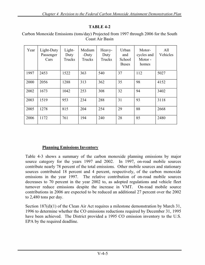
Chapter 4 Revision to the Federal Carbon Monoxide Attainment Demonstration Plan
V-4-5
TABLE 4-2 Carbon Monoxide Emissions (tons/day) Projected from 1997 through 2006 for the South
Coast Air Basin
Year Light-Duty Passenger
Cars
Light-Duty
Trucks
Medium-Duty Trucks
Heavy-Duty
Trucks
Urban and
School Buses
Motor-cycles and
Motor -homes
All Vehicles
1997 2453 1522 363 540 37 112 5027
2000 2056 1288 313 362 35 98 4152
2002 1673 1042 253 308 32 94 3402
2003 1519 953 234 288 31 93 3118
2005 1278 815 204 254 29 88 2668
2006 1172 761 194 240 28 85 2480
Planning Emissions Inventory
Table 4-3 shows a summary of the carbon monoxide planning emissions by major source category for the years 1997 and 2002. In 1997, on-road mobile sources contribute nearly 78 percent of the total emissions. Other mobile sources and stationary sources contributed 18 percent and 4 percent, respectively, of the carbon monoxide emissions in the year 1997. The relative contribution of on-road mobile sources decreases to 70 percent in the year 2002 to, as adopted regulations and vehicle fleet turnover reduce emissions despite the increase in VMT. On-road mobile source contributions in 2006 are expected to be reduced an additional 27 percent over the 2002 to 2,480 tons per day.
Section 187(d)(1) of the Clean Air Act requires a milestone demonstration by March 31, 1996 to determine whether the CO emissions reductions required by December 31, 1995 have been achieved. The District provided a 1995 CO emission inventory to the U.S. EPA by the required deadline.
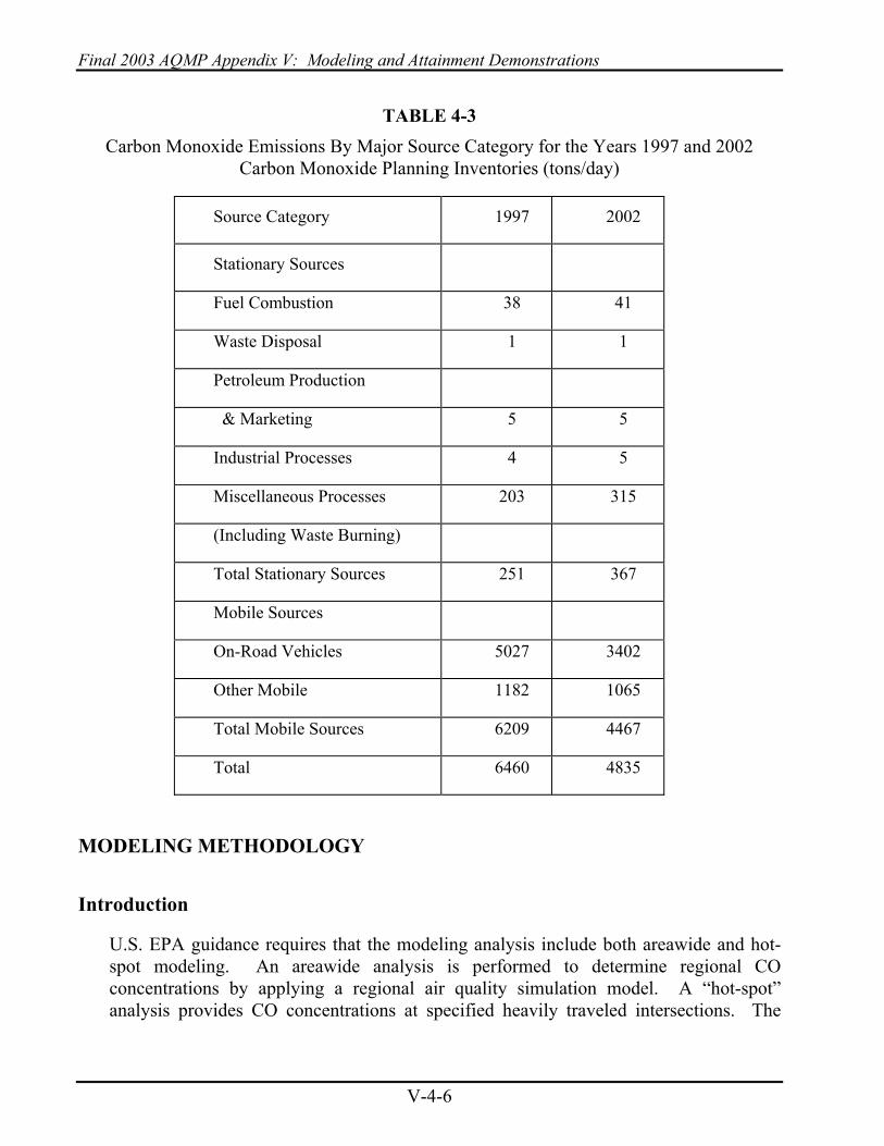
Final 2003 AQMP Appendix V: Modeling and Attainment Demonstrations
V-4-6
TABLE 4-3 Carbon Monoxide Emissions By Major Source Category for the Years 1997 and 2002
Carbon Monoxide Planning Inventories (tons/day)
Source Category 1997 2002
Stationary Sources
Fuel Combustion 38 41
Waste Disposal 1 1
Petroleum Production
& Marketing 5 5
Industrial Processes 4 5
Miscellaneous Processes 203 315
(Including Waste Burning)
Total Stationary Sources 251 367
Mobile Sources
On-Road Vehicles 5027 3402
Other Mobile 1182 1065
Total Mobile Sources 6209 4467
Total 6460 4835
MODELING METHODOLOGY
Introduction
U.S. EPA guidance requires that the modeling analysis include both areawide and hot-spot modeling. An areawide analysis is performed to determine regional CO concentrations by applying a regional air quality simulation model. A “hot-spot” analysis provides CO concentrations at specified heavily traveled intersections. The

Chapter 4 Revision to the Federal Carbon Monoxide Attainment Demonstration Plan
V-4-7
2003 revision to the CO Plan uses Comprehensive Air Quality Model with Extensions (CAMx) air quality simulation model to assess regional CO concentrations and CAL3QHC to perform the hot-spot analysis. This chapter describes the carbon monoxide (CO) modeling approach used to demonstrate attainment of the federal 8-hour CO standard of 9.5 ppm. The 1992 CO Plan and 1994 AQMP provide additional supporting documentation describing the modeling procedures.
Regional Modeling Analysis
The October 31-November 1, 1997 meteorological episode resulted in the Basin’s highest measured 8-hour average carbon monoxide concentration (17 ppm) since 1996. The peak concentration was measured at the Lynwood, the air monitoring station that has historically measured the Basin’s highest CO concentrations and the greatest frequency of days exceeding the federal standard. The two-day episode took place during mid-fall on a Friday night and Saturday morning under very stagnant conditions. The episode took place on the weekend following the reversion to standard time. The following sections describe the meteorological and air quality characteristics of the October 31-November 1, 1997 August 1997 episode, the input preparation procedures used to develop the model input file for CAMx, and the respective model performance.
Episode Selection
For the 2003 revision to the CO Plan, the October 31-November 1, 1997 carbon monoxide meteorological episode replaces the December 1989 episode. The episode was selected for three principal reasons. First, the episode is more recent that the December 1989 episode that occurred over ten year ago. EPA’s guidance for regional modeling recommends the use of meteorological episodes for air quality attainment demonstrations that are less than ten years old to ensure consistency in the trends of emissions. The 1997 episode occurred after the 1996 California Phase II fuel reformulation program in a period where the fuel is consistent with that used in 2002, the year selected for this attainment demonstration. Second, the October 31-November 1, 1997 episode measured the second highest 8-hour average carbon monoxide concentrations in the Basin since fuel reformulation was implemented. (On January 12, 1996, a 17.3 ppm 8-hour average CO concentration was measured at Lynwood). Third, episode took place during the SCOS97 monitoring program, with its enhanced network of surface and upper air meteorological monitoring. The SCOS97 monitoring was designed specifically to provide the data requirement for sate-of-the-art regional air quality models.
Basin carbon monoxide episodes typically occur during the months of December and January during long cold nights that enhance nocturnal inversions creating a very stable

Final 2003 AQMP Appendix V: Modeling and Attainment Demonstrations
V-4-8
environment. The episodes fall into two categories: a one-day morning peak that builds in the early morning hours and is enhanced by morning rush hour emissions. The second type of episode spans two days, commencing at the evening rush hour and building through the night into the following morning. The peak concentrations are often measured around midnight, gradually falling through the early morning hours on the second day. The severity of the episode is defined as the combination of local emissions being enhanced by the regional re-circulation of urban, carbon monoxide emissions from the Central Los Angeles metropolitan area back to the South Central Los Angeles area. The December 1989 episode, analyzed in the 1994 and 1997 CO Plan is characteristic of the 2-day episode. The October 31-November 1, 1997 episode is also in this category.
A statistical model was developed to better characterize the October 31-November 1, 1997 episode relative to the seven year post fuel reformulation period. Multi-variate regression was conducted using 8-hour average concentrations of Lynwood carbon monoxide and surface and upper air meteorological data for 1996. The equation developed from the analysis was applied to the meteorological data for the seven-year period to predict Lynwood carbon monoxide and establish a daily ranking. The log linear regression included surface pressure gradient data (wind forcing), the vertical temperature structure of the near surface boundary layer and the number of hours of daylight. The October 31-November 1, 1997 episode ranked in the 94th percentile of the distribution (2557 cases). However when the number of hours in the day were normalized for all days to reflect the October 31-November 1, 1997 period the ranking reaches the 98th percentile and is equivalent to that of January 12, 1996 when the peak carbon monoxide concentration was observed for the seven year period. For reference, January 8, 2002, the last day that 8-hour average carbon monoxide concentrations exceeded the standard ranked in the 95th percentile of the distribution.
The meteorological profile characterizing the top ranked carbon monoxide days is provided in Table 4-4. In general, high carbon monoxide concentrations occur when summer strength high pressure aloft envelops the Basin coupled with offshore pressure gradients that stagnate local winds. The upper level high acts to enhance the nocturnal radiation inversion, effectively restricting air flow to a shallow layer near the ground. The offshore tendency in the pressure gradients act to stagnate the see breeze early in the afternoon and direct the regional drift of urban carbon monoxide south from Central Los Angeles.
Episode Characterization
The meteorological setting characterizing the October 31-November 1, 1997 episode has been characterized as a part of the SCOS97 monitoring program. The episode has been documented in a special edition of Atmospheric Environment through a special

Chapter 4 Revision to the Federal Carbon Monoxide Attainment Demonstration Plan
V-4-9
secession of the AWMA Annual Conference, held in San Diego, June 1999. The following subsections examine the observed synoptic and mesoscale meteorological profiles as well as the carbon monoxide air quality that was measure during the October 31-November 1, 1997 episode.
Table 4-4
Meteorological Profile of High Carbon Monoxide Episodes
Variable Value Std. Dev Units Time
VBG 500 Mb Pressure Surface Height 5823 54 M 0400 PST
Summation Surface Pressure Gradient
[LGB-DAG+RIV-DAG+SAN-LAS]
-18.9 4.9 Mb 0700 PST
LAX-SFO Surface Pressure Gradient -4.5 2.1 Mb 0700 PST
950 Mb Temperature 17.8 3.0 oC 0400 PST
Inversion Top Temperature 18.7 3.7 oC 0400 PST
Inversion Strength 7.4 2.9 oC 0400 PST
Synoptic Setting
A strong ridge of high pressure aloft developed over the west coast of California during the last week in October, 1997 and remained in place into the first week of November 1997. The ridge strengthened significantly between the morning (0400 PST)of October 30th and the same time on the 31st with the height of the 500 mb level increasing approximately 70 m in a 24 hour period. The center of the high measure 5930 m located over the Southern California bight, positioned to bring the maximum level of subsidence to the Basin, enhancing the nocturnal inversion. (The 5920 m height at the 500 Mb pressure surface measured at Vandenburg Air Force Base is two standard deviations above the average defining the high carbon monoxide episodes). Figure 4-1 illustrates the upper level pattern observed on October 31, 1997.
Mesoscale Setting
The mesoscale setting for the October31-November 1, 1997 episode was dominated by developing offshore pressure gradients characterized by high pressure building into the Great Basin and a local thermal trough off the San Diego Coast. Figure 4-2 depicts the

Final 2003 AQMP Appendix V: Modeling and Attainment Demonstrations
V-4-10
2200 PST surface pressure analysis for October 31, 1997. The orientation of the pressure gradient was from north to south with summation pressure gradients increasing offshore from –5.9 Mb at 0700 PST on the 31st to –14.2 Mb at 0700 PST on the 1st. The net result of the increasing offshore gradients was to stagnate winds in the coastal portion of the Basin in the early evening. Velocities at most of the stations registered calm or 1-2 mph. Only a weak northeast to southwest gradient flow was observed throughout the night generating a mass drift from Central LA and the south San Gabriel Valley back towards Lynwood following the Los Angeles and San Gabriel River valleys. (The Los Angeles and San Gabriel River valleys are typically identified by the river channels and are bordered by a moderate elevation gain in the terrain to the west of the City of Lynwood).
Figure 4-1
500 Mb Pressure surface contour patterns on Friday October 31, 1997 at 0400 PST
The nocturnal inversion that developed over the Basin was greatly enhanced by the subsidence from aloft. The temperature measured at the at 950 Mb level from the San Diego sounding at 0400 PST on November 1st reached 26.8 oC while the inversion top temperature reached 28 oC. . The inversion strength calculated for coastal Southern California was 11.9 oC. In all, the vertical temperature structure was at a minimum of one to two standard deviations more stagnant than the typical carbon monoxide episode.

Chapter 4 Revision to the Federal Carbon Monoxide Attainment Demonstration Plan
V-4-11
Figure 4-2
Surface Pressure Analysis on Friday October 31, 1997 at 2200 PST
Air Quality Setting
The air quality profile that emerged during the October 31-November 1, 1997 episode followed the meteorological setting for local stagnation being enhance by regional drift of carbon monoxide from the Central L.A. (downtown) area. Carbon monoxide concentrations were background during the afternoon hours of October 31st but began to rise as the sunset and the Friday traffic phased into rush hour. Hourly averaged concentrations climbed to approximately 9 ppm throughout the coastal plain by midnight on October 31st with carbon monoxide levels reaching a peak 1-hour level of 19 ppm at Lynwood. The rise (approximately 4 ppm per hour) in CO at Lynwood occurred through local emissions from the surrounding freeways and major arterial and from the emissions that drain through the coastal plain.
By midnight, concentrations of carbon monoxide began to fall at Central LA, Pico Rivera West L.A. and the San Fernando Valley air monitoring stations. Concentrations at Lynwood held steady for three hours while carbon monoxide at Hawthorne rose through 0600 PST on November 1st. The maximum 8- hour average at Lynwood reached 17.0 ppm at 0400 PST on November 1st and Hawthorne reached 10 ppm at 0700 PST.

Final 2003 AQMP Appendix V: Modeling and Attainment Demonstrations
V-4-12
Model Selection
CAMx was selected for the regional modeling demonstration. CAMx is a state-of-the-art regional photochemical model that uses multiple terrain following layers with fixed thickness, and the Bott advection solver for mass transport. The CAMx carbon monoxide simulations were run with the Carbon Bond IV (CB-IV) chemistry module using full chemistry. The MM5 prognostic and CALMET meteorological models were used to generate objective/diagnostic wind and mixing fields for the analysis. Estimates of horizontal and vertical diffusivity were generated from the CALMET meteorological fields as input to the modeling simulation. The simulations were run on the SCOS97 modeling domain (see Figure 4-3) using a five kilometer squared grid.
Meteorological Modeling and Input Fields
Meteorological modeling was performed by coupling the meteorological fields generated from the MM5 prognostic model with objective data and diagnostic options of the CALMET meteorological model. The output of the MM5 prognostic meteorological model was used as a “first guess” wind assumption for the CALMET simulation. Observational data used to drive the simulation was acquired from the SCOS97 field-monitoring program. CALMET was run using 17 vertical layers with the lowest layer consisting of 20 m in depth. Wind and temperature data were mapped to CAMX using layer interpolation.
Hourly upper air temperature and wind data measured at twelve radar wind profiler and radio acoustic sounding systems (RWP/RASS) augmented the twice daily routine rawindsonde profiles measured at Vandenburg Air Force Base and Miramar Naval Air Station. The RWP/RASS measure winds to three kilometers above ground level (AGL) at approximately 150 m range gates. Temperature profiles routinely reached one kilometer AGL at the same measurement levels.
Surface wind, temperature and humidity and cloud cover data from 238 monitoring sites comprised the basis of the surface meteorological fields. The data incorporated measurements from several monitoring networks including the District, Ventura County APCD, San Diego County APCD, California Irrigation Management System (CIMIS), FAA's METAR, Remote Automatic Weather System (RAWS), National Parks Networks (NPS) and Bureau of Land Management (BLM) networks. Figure 4-3 shows the location of surface meteorological stations.
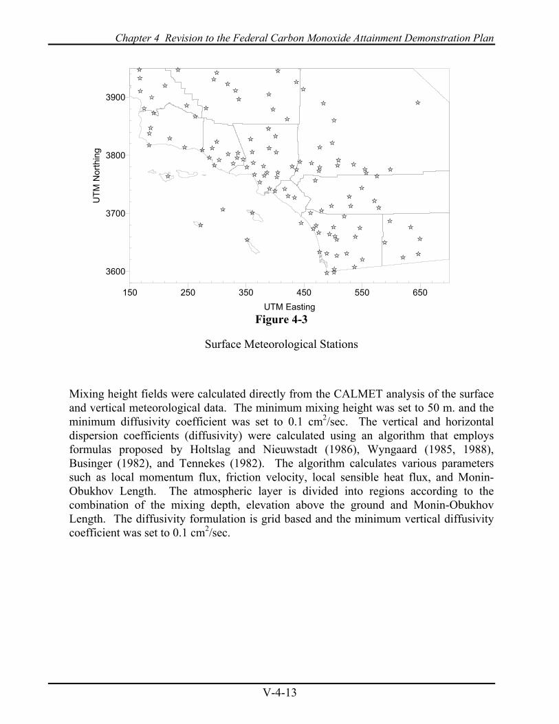
Chapter 4 Revision to the Federal Carbon Monoxide Attainment Demonstration Plan
V-4-13
150 250 350 450 550 650UTM Easting
3600
3700
3800
3900U
TM N
orth
ing
Figure 4-3
Surface Meteorological Stations
Mixing height fields were calculated directly from the CALMET analysis of the surface and vertical meteorological data. The minimum mixing height was set to 50 m. and the minimum diffusivity coefficient was set to 0.1 cm2/sec. The vertical and horizontal dispersion coefficients (diffusivity) were calculated using an algorithm that employs formulas proposed by Holtslag and Nieuwstadt (1986), Wyngaard (1985, 1988), Businger (1982), and Tennekes (1982). The algorithm calculates various parameters such as local momentum flux, friction velocity, local sensible heat flux, and Monin-Obukhov Length. The atmospheric layer is divided into regions according to the combination of the mixing depth, elevation above the ground and Monin-Obukhov Length. The diffusivity formulation is grid based and the minimum vertical diffusivity coefficient was set to 0.1 cm2/sec.

Final 2003 AQMP Appendix V: Modeling and Attainment Demonstrations
V-4-14
Trajectory Analysis
Figures 4-4 through 4-7 depict the time series (3-hour intervals, beginning at 1500 PST) of carbon monoxide transport simulated using the MM5/CALMET wind fields. The trajectory illustrates the transport of carbon monoxide emissions injected into the Central L.A. grid and it movement during the early evening-late night hours of October 31st. The simulation illustrates the ability of the wind field to characterize the regional drift of carbon monoxide that contributed to background concentrations at Lynwood that night and the following morning.
CAMx Initial and Boundary Conditions
Initial conditions used by the CAMx simulation were derived from hourly observational data measured by the District and neighboring air quality agencies. The lateral boundary and top boundaries were set at “EPA Clean” North American continental average concentrations. Table 4-5 summarizes the species concentrations.
Base Year Emissions
The 1997 base year emissions inventory totaled 6425 tons of carbon monoxide per day. The total is approximately 35 tons lower that the 1997 tonnage listed in the planning inventory. The modeling inventory reflects day specific ambient temperature corrections made to mobile and other source operating conditions.
Day-of-Week Diurnal Traffic Patterns
One additional import segment of data acquired as part of the SCOS97 monitoring program was the hourly vehicle count data monitored in Basin by the 11 Caltrans weigh- in-motion (WIM) stations. The hourly vehicle count profiles were day and location specific. The profiles were collected over during the course of the SCOS97 program and were aggregated into typical day-of-week patterns. The day pattern stratifies vehicle counts by hour and provides an improved characterization of the diurnal traffic patterns. The data is expressed as an hourly frequency of the total daily vehicle use (e.g. hour 0-1 2 percent of the total traffic volume fro the 24-hour period). The vehicle count data illustrates the different traffic patterns observed on weekdays (Thursday is used as a surrogate), Friday and Saturday. Figure 4-8 illustrates the Thursday, Friday and Saturday patterns for vehicle use by hour of day. This data was used to refine the traffic patterns defined by the DTIM4 transportation model.

Chapter 4 Revision to the Federal Carbon Monoxide Attainment Demonstration Plan
V-4-15
Figure 4-4 Simulated Carbon Monoxide Tracer Release 1500 PST, October 31, 1997
Figure 4-5
Simulated Carbon Monoxide Tracer Release 1800 PST, October 31, 1997

Final 2003 AQMP Appendix V: Modeling and Attainment Demonstrations
V-4-16
Figure 4-6 Simulated Carbon Monoxide Tracer Release 2100 PST, October 31, 1997
Figure 4-7
Simulated Carbon Monoxide Tracer Release 2300 PST, October 31, 1997

Chapter 4 Revision to the Federal Carbon Monoxide Attainment Demonstration Plan
V-4-17
0
2
4
6
8
1 4 7 10 13 16 19 22
ThursFriSat
% Hrs In Day
Figure 4-8
Diurnal Vehicle Usage Distribution from Caltrans Weigh-In-Motion Station Data
Base Year Model Performance
Table 4-6 shows the performance statistics for the CAMx simulation using the 1997 baseline emissions inventory. Shown in Table 4-6 are the paired peak prediction accuracy (paired in space) and U.S. EPA-suggested two statistical performance measures. The accuracy of the peak 8-hour average prediction was -12 percent and -24 percent for unpaired and paired peak prediction, respectively. The paired absolute error marginally exceeds the performance goal of 25 to 30 percent. The simulation is within the temporal absolute error of two hours.

Final 2003 AQMP Appendix V: Modeling and Attainment Demonstrations
V-4-18
Table 4-5
EPA Clean Top and Lateral Boundary Concentrations
Species Concentration(ppm) NO 0.0010000 NO2 0.0020000 O3 0.0400000 OLE 0.0002760 PAR 0.0137000 TOL 0.0001640 XYL 0.0000900 FORM 0.0019280 ALD2 0.0005080 ETH 0.0004680 CRES 0.0000100 OPEN 0.0000100 PNA 0.0000100 NXOY 0.0000100 NO3 0.0000100 PAN 0.0000100 CO 0.2000000 HONO 0.0000100 H2O2 0.0000100 HNO3 0.0000100 SO2 0.0100000 SO4 0.0001000 AERO 3.0000000

Chapter 4 Revision to the Federal Carbon Monoxide Attainment Demonstration Plan
V-4-19
TABLE 4-6 Performance Statistics for the October 31-November 1, 1997 CO Episode
Performance Measure CAMx U.S. EPA-Suggested Measures
Peak 8-Hour Station Prediction 13.0 ppm -- Peak 8-Hour Regional Prediction 14.9 ppm -- Peak 8-Hour Measurement 17.0 ppm -- Paired Highest 8-Hour Prediction Accuracy
-24% --
Unpaired Highest 8- Hour Prediction Accuracy
-12 % +/- 30-35 %
Average Absolute Error in 8-Hour Peak Prediction
39 % 25-30 %
Average Absolute Error in the Predicted Time of the 8-Hour Peak Concentration for Station Pairs > 5.0 ppm
1.6 hours 2 hours
Figures 4-11 and 4-12 provide the temporal station model carbon monoxide performance for the coastal Basin stations for the 1-hour and 8-hour average concentrations respectively. The solid line depicts the predicted trend with observations depicted as squares. The CAMx simulation captures the diurnal trend observed at Lynwood during the night of October 31st and morning of November 1st. The general tendency for the model is to under-predict regional carbon monoxide concentrations. However, this tendency is consistent with the use of a 5 kilometer grid where emissions and transported carbon monoxide is uniformly distributed throughout the grid.
Figures 4-13 through 4-16 present the CAMx predicted carbon monoxide spatial distribution for 1500, 1800, 2100 and 2300 PST on October 31, 1997. As is depicted in the sequence, carbon monoxide builds from the early evening, peaking over South Central Los Angeles near midnight. The carbon monoxide levels also rise throughout the Basin and Ventura and San Diego in response to the stagnant conditions.

Final 2003 AQMP Appendix V: Modeling and Attainment Demonstrations
V-4-20
Figure 4-11
CAMx Simulated vs. Observed 1-hour Average Carbon Monoxide for the October 31-November 1, 1997 Meteorological Episode

Chapter 4 Revision to the Federal Carbon Monoxide Attainment Demonstration Plan
V-4-21
Figure 4-12
CAMx Simulated vs. Observed 8-hour Average Carbon Monoxide for the October 31-November 1, 1997 Meteorological Episode

Final 2003 AQMP Appendix V: Modeling and Attainment Demonstrations
V-4-22
Figure 4-13
CAMx Simulated Regional Carbon Monoxide 1500 PST, October 31, 1997
Figure 4-14
CAMx Simulated Regional Carbon Monoxide 1800 PST, October 31, 1997

Chapter 4 Revision to the Federal Carbon Monoxide Attainment Demonstration Plan
V-4-23
Figure 4-15
CAMx Simulated Regional Carbon Monoxide 2100 PST, October 31, 1997
Figure 4-16 CAMx Simulated Regional Carbon Monoxide 2300 PST, October 31, 1997
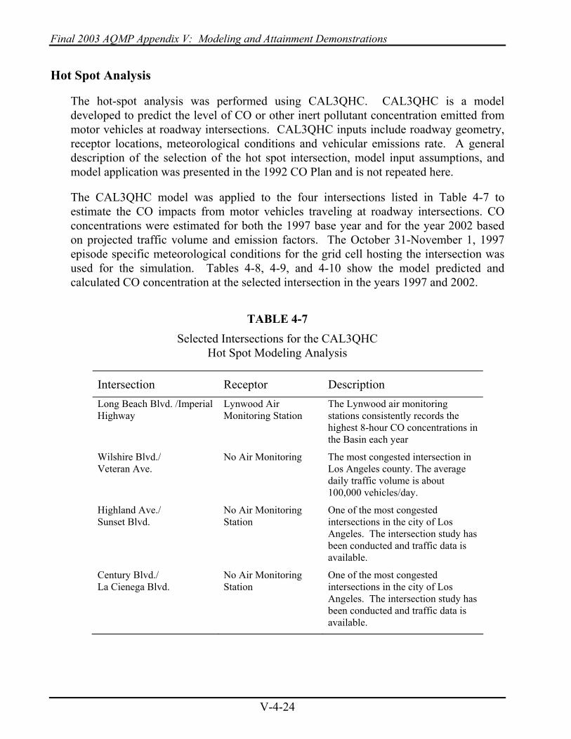
Final 2003 AQMP Appendix V: Modeling and Attainment Demonstrations
V-4-24
Hot Spot Analysis
The hot-spot analysis was performed using CAL3QHC. CAL3QHC is a model developed to predict the level of CO or other inert pollutant concentration emitted from motor vehicles at roadway intersections. CAL3QHC inputs include roadway geometry, receptor locations, meteorological conditions and vehicular emissions rate. A general description of the selection of the hot spot intersection, model input assumptions, and model application was presented in the 1992 CO Plan and is not repeated here.
The CAL3QHC model was applied to the four intersections listed in Table 4-7 to estimate the CO impacts from motor vehicles traveling at roadway intersections. CO concentrations were estimated for both the 1997 base year and for the year 2002 based on projected traffic volume and emission factors. The October 31-November 1, 1997 episode specific meteorological conditions for the grid cell hosting the intersection was used for the simulation. Tables 4-8, 4-9, and 4-10 show the model predicted and calculated CO concentration at the selected intersection in the years 1997 and 2002.
TABLE 4-7 Selected Intersections for the CAL3QHC
Hot Spot Modeling Analysis
Intersection Receptor Description Long Beach Blvd. /Imperial Highway
Lynwood Air Monitoring Station
The Lynwood air monitoring stations consistently records the highest 8-hour CO concentrations in the Basin each year
Wilshire Blvd./ Veteran Ave.
No Air Monitoring The most congested intersection in Los Angeles county. The average daily traffic volume is about 100,000 vehicles/day.
Highland Ave./ Sunset Blvd.
No Air Monitoring Station
One of the most congested intersections in the city of Los Angeles. The intersection study has been conducted and traffic data is available.
Century Blvd./ La Cienega Blvd.
No Air Monitoring Station
One of the most congested intersections in the city of Los Angeles. The intersection study has been conducted and traffic data is available.

Chapter 4 Revision to the Federal Carbon Monoxide Attainment Demonstration Plan
V-4-25
TABLE 4 -8 Emissions Predicted by EMFAC2002 in Year 1997 and 2002
Wilshire - Veteran Sunset - Highland La Cienega - Century Long Beach - Imperial AM PM AM PM AM PM AM PM
a) EMFAC2002 Emission Variables (1997)
Running Exhaust Emission Factor
(g/mile)
11.57 11.96 13.31 12.72 11.82 11.66 11.92 11.93
Idling Emission Factor (g/min)
2.13 2.18 2.43 2.32 2.19 2.15 2.22. 2.18
b) EMFC2002 Emission Variables (2002)
Running Exhaust Emission Factor
(g/mile)
7.20 7.21 7.22 7.98 7.31 7.24 7.35 7.48
Idling Emission Factor (g/min)
1.24 1.24 1.25 1.30 1.27 1.25 1.28 1.28
TABLE 4-9 1997 1-Hour Average Carbon Monoxide Concentrations
Calculated from the CAL3QHC Model
Morning* Afternoon+ Peak++
Wilshire - Veteran
7.7 5.7 --
Sunset - Highland 6.9 7.3 --
La Cienega - Century
6.4 5.2 --
Long Beach - Imperial
5.1 5.2 2.2
* Morning : 7-8 a.m. for La Cienega - Century, 11-12 a.m. for Sunset - Highland, 8-9 for Wilshire-Veteran, and 7-8 a.m. for Long Beach - Imperial
+ Afternoon : 3-4 p.m. for Sunset - Highland, 3-4 p.m. for Wilshire - Veteran, 4-5 p.m. for Long Beach - Imperial, and 6-7 p.m. for La Cienega - Century
++ Peak : 11-12 p.m. (concentration at the hour of the observed peak). Peak is only provided for the Long Beach/Imperial intersection since it is intersection associated with the regional peak at Lynwood.

Final 2003 AQMP Appendix V: Modeling and Attainment Demonstrations
V-4-26
TABLE 4-10 Year 2002 1-Hour Average Carbon Monoxide Concentrations
Calculated from the CAL3QHC Model
Morning* Afternoon+ Peak++
Wilshire-Veteran 4.6 3.5 --
Sunset-Highland 4.0 4.5 --
La Cienega-Century 3.7 3.1 --
Long Beach-Imperial 3.0 3.1 1.2
* Morning : 7-8 a.m. for, La Cienega - Century, 8-9 a.m. for Wilshire - Veteran, 7-8 a.m. for Long Beach - Imperial, and 8-9 a.m. for Sunset - Highland
+ Afternoon : 3-4 p.m. for Sunset - Highland, 5-6 p.m. for Wilshire - Veteran, 4-5 p.m. and Long Beach - Imperial, and. 6-7 p.m. for and La Cienega - Century
++ Peak : 11-12 p.m. (concentration at the hour of the observed peak) ). Peak is only provided for the Long Beach/Imperial intersection since it is intersection associated with the regional peak at Lynwood.
CARBON MONOXIDE CONTROL STRATEGY
Mobile sources, which are regulated primarily by ARB or U.S. EPA, produce the largest amount of carbon monoxide emissions in the Basin. The on-road motor vehicle control strategy is primarily based on adopted regulations, such as the 1990 ARB Low-Emission Vehicles and Clean Fuels (LEV/Clean Fuels) regulations, Phase 2 Reformulated Gasoline Program, oxygenated fuel regulation, and enhancements to the Inspection and Maintenance (I/M) or Smog Check program. The emission reduction resulting from these already adopted regulations are sufficient to demonstrate attainment in the year 2002, as discussed in a later section.
Contingency Measures
Section 187(a)(3) of the 1990 CAAA requires that adopted and enforceable contingency measures be included in the attainment plan submission. A deviation from the forecasted VMT of more than a given percentage will trigger implementation of contingency measures to offset either excess VMT or carbon monoxide emissions due to the additional VMT. According to the EPA General Preamble [Sect. 532(c)(1)], this percentage is 5 percent in 1994, 4 percent in 1995, and 3 percent for 1996 and subsequent years. The cumulative VMT growth cannot be greater than or equal to 5 percent above the VMT forecast used as the basis of the attainment demonstration.

Chapter 4 Revision to the Federal Carbon Monoxide Attainment Demonstration Plan
V-4-27
District Rule 1504 was adopted to serve as contingency for carbon monoxide. Table 4-11 lists the control measures that will also serve as contingency measures for carbon monoxide. These measures are described further in Appendix IV-A of the 1997 AQMP.
TABLE 4-11 Level I - Contingency Measures from the 1997 AQMP Which May Serve as Carbon
Monoxide Contingency Measures
AQMP Measure Number
Title Priority to Meet CAA
Requirements
Responsible Agency
Issues
CTY-4 Enhanced Oxygenated Fuel Content for CO
1 ARB Potential NOx Emission Increases
CTY-1 Accelerated Implementation of Control Measures
2 District Resource Availability
CTY-2 Command and Control Rules in
Place of Educational Outreach Program
Measures
3 District Resource Availability/
Cost Effectiveness
FUTURE AIR QUALITY PROJECTIONS
Introduction
Air quality modeling is an integral part of the planning process to achieve clean air. Based on U.S. EPA’s modeling guidelines, CAMx is used for the areawide analysis, and CAL3QHC, a roadway intersection model, is used to calculate carbon monoxide concentrations near intersections. The CAMx model results are used to evaluate the effectiveness of control measures in attaining the federal 8-hour air quality standard for carbon monoxide in the year 2002. U.S. EPA’s modeling guidelines recommend that the results from CAL3QHC and CAMx be combined to give a total concentration that is used for attainment demonstration purposes. However, conclusions from a 1989 study, conducted by ARB and the District in the vicinity of the Lynwood area, indicate that the areawide and ‘hot-spot’ model results should not be combined. The study indicates that the CO measurements at the Lynwood monitoring station are representative of the entire Lynwood area. Based on the conclusions of the Lynwood study, the areawide analysis and the “hot-

Final 2003 AQMP Appendix V: Modeling and Attainment Demonstrations
V-4-28
spot” analysis results for the attainment demonstration are not combined. A more detailed discussion of this subject can be found in the 1992 CO Plan.
Emissions
The 2002 modeling emission inventory consists of area, point and mobile sources. More than 90 percent of CO emissions are from mobile sources. Area source and point source CO emissions are only 9 percent of the total inventory. The carbon monoxide modeling analysis for the Basin uses a grid level emission inventory representing day-specific mobile source emissions.
The 1997 and 2002 carbon monoxide emissions used in the CAMx modeling analysis are shown in Table 4-12. The emissions estimates include the emission reductions from all air quality rules and regulations adopted prior to September 30, 2002, including the effect of the enhanced I/M program and the oxygenated fuel regulation. The emissions presented in this table reflect the revised VMT forecast from SCAG and the latest version of ARB’s on-road emission factor program, EMFAC2002.
TABLE 4-12 Baseline and Projected Future Basin Carbon Monoxide Emissions (tons/day)
Case On-Road Mobile
Others Total
1997 5223 1202 6425
2002 3259 1116 4375
Modeling Results
CAMx Regional Simulation
Table 4-13 presents the projected carbon monoxide concentrations for the Basin and at the Lynwood station in the years 1997 and 2002. The predicted maximum 8-hour concentration of 14.9 ppm occurred in the Lynwood area at the same time (0400 PST) as the measured maximum 8-hour concentration of 17.0 ppm on November 1, 1997. The predicted maximum 8-hour concentration is within the model peak performance goal recommended by the U.S. EPA. The predicted regional 1-hour average concentration is 16.7 whereas the observed value was 19 ppm. The maximum predicted 8-hour carbon monoxide concentration at the Lynwood station is 13.0 ppm.

Chapter 4 Revision to the Federal Carbon Monoxide Attainment Demonstration Plan
V-4-29
TABLE 4-13 Peak Carbon Monoxide Concentrations (ppm) Predicted by CAMx for the Basin
Scenario Regional Maximum
(8-hour Average)
Maximum Lynwood
(8-hour Average)
Regional Maximum
(1-hour Average)
1997 Base 14.9 13.0 16.7
2002 Base 9.9 8.7 10.8
Note: Federal Standards: 9.5 ppm, 8-hour average; 35 ppm, 1-hour average
In the 2002 modeling analysis the predicted regional maximum 8-hour average concentration is reduced by 34 percent from 1997 to 9.9 ppm. The 2002 predicted 8-hour average concentration at the Lynwood monitor is reduced by 33 percent to 8.7 ppm. The regional maximum 1-hour average concentration drops by 36 percent in 2002 to 10.8 ppm. The time of the peak 8-hour averages (both regional and at Lynwood) remained at 0400 PST.
The carbon monoxide air quality projections are based on CAMx and CAL3QHC simulations analyses for the fall meteorological episode. The October 31-November 1, 1997 episode recorded maximum 1-hour and 8-hour average carbon monoxide concentrations of 19.0 ppm and 17.0 ppm, respectively. These were the highest recorded values in the Basin since 1996. The 2002 predicted 8-hour average maximum concentration closely matches the maximum observed carbon monoxide concentration measured at Lynwood in 2002 (10.1 ppm on January 8th). However, the concentration exceeds the federal and state levels by a marginal amount.
Linear Rollback of CAMx Simulation Results
Figure 4-17 depicts the trend of EMFAC2002 projected carbon monoxide emissions for 1997 through 2005. On-road CO emissions from vehicles that are the primary contributors to urban carbon monoxide episodes are projected to decrease by an average of seven percent per year in 2003 through 2005. Total CO emissions reductions for all categories are projected to be reduced between 5 and 6 percent per year through 2005.
A linear rollback approach is used to evaluate CO concentrations beyond 2002. It assumes that the ambient concentrations above background levels are directly proportional to the emissions in the immediately adjacent areas. With CO being essentially inert, this assumption is reasonable. In mathematical terms, the rollback relationship can be written as follows:

Final 2003 AQMP Appendix V: Modeling and Attainment Demonstrations
V-4-30
Cp = [(Cb - k) • Qp/Qb] + k
where Cp and Cb are the future year and baseline CO concentrations, respectively; Qp and Qb are the future year and baseline CO emission rates, respectively; and k denotes the global background CO concentration. It is assumed that global background CO concentrations are negligible; therefore the above equation simplifies to
Cp = Cb • Qp/Qb
For the 2003 AQMP CO attainment demonstration, linear roll back is used to extend the CAMx simulated regional maximum 8-hour average concentration beyond 2002 to predict carbon monoxide concentrations for 2003, 2004 and 2005. Using linear rollback, the CAMx 2002 base year simulation and the projected reduction in CO emissions, the predicted carbon monoxide maximum 8-hour concentration is expected to be reduced to 9.1 ppm in 2003, 8.4 ppm in 2004 and 7.8 ppm in 2005. The continued reductions in carbon monoxide emissions are expected to maintain the attainment of the federal 8-hour standard demonstrated through observations in 2001 and 2002. The California 8-hour average carbon monoxide standard is projected to be met in 2004. The results are summarized in Table 4-14.
0
1000
2000
3000
4000
5000
6000
1997 1998 1999 2000 2001 2002 2003 2004 2005
(TPD)
FIGURE 4-17 EMFAC2002 Projected On-Road Carbon Monoxide Emissions for 1997 Through 2005

Chapter 4 Revision to the Federal Carbon Monoxide Attainment Demonstration Plan
V-4-31
TABLE 4-14
Carbon Monoxide Emissions and Model-Predicted Concentrations
CO-Planning 8-hr Maximum 1-hr MaximumYear/Scenario Inventory Concentration Concentration
(tons/day) (ppm) (ppm) 1997 Baseline
6460 14.9 16.7
2002 Baseline
4835 9.9 10.8
2003 Predicted
4527 9.1 9.9
2004 Predicted 4278 8.4 9.2 2005 Predicted 4029 7.8 8.5
State 1-hr CO standard = 20 ppm State 8-hr CO standard = 9.0 ppm Federal 8-hr CO standard = 9.5 ppm
CAL3QHC Modeling Results and Combined “Hot Spot” and Areawide Maximum Analysis
The maximum CAL3QHC 8-hour average concentrations projected at the four roadway intersections (regardless of time of day) and the CAL3QHC 8-hour average concentrations projected for the hour coincident with the occurrence of the CAMx simulated area-wide maximum impact are presented in Table 4-15. Also presented are the CAMx projected area-wide maximum concentrations for the grid cell hosting the intersection and the sum of the CAMx projected area-wide maximum and the CAL3QHC 8-hour average concentrations projected for that hour. Linear rollback is used to extend the CAL3QHC "hot spot" intersection and the CAMx area-wide grid cell simulations from 2002 through 2005. The CAL3QHC analysis was conducted using the actual meteorological conditions for the episode. It should be noted that the projected maximum concentrations from the CAMx and CAL3QHC do not occur at the same time of the day and cannot be directly added. (The “hot spot” predicted carbon monoxide 8-hour average maximum concentrations at the intersections occurred between 1200 and 1400 PST).
Projected maximum “hot-spot” concentrations in the year 2002 are between 2.3 and 3.8 ppm. CAMx projected area-wide carbon monoxide peak 8-hour average concentrations (for the grid cell hosting the intersection) in the year 2002 are between 1.6 and 9.2 ppm. The highest CAMx simulated 8-hour carbon monoxide concentration occurs at Lynwood, the highest “hot-spot” concentration does not occur at Lynwood, but at intersections in Hollywood and Westwood. The maximum eight hour average “hot-spot” concentration

Final 2003 AQMP Appendix V: Modeling and Attainment Demonstrations
V-4-32
predicted for the intersection of Imperial and Long Beach Blvd. at the time of the observed maximum (0600 PST) values 0.8 ppm.
Adding the 2002 Lynwood 0600 PST 8-hour average “hot spot” intersection impact to the CAMx predicted 0600 PST 8-hour average for the grid cell hosting the Lynwood monitoring station results in a total impact of 10.0 ppm. This value is close to the 2002 observed maximum 8-hour average concentration (10.7 ppm) at Lynwood on January 8th (meteorologically ranked 95th percentile, or an expected frequency of occurrence on 15 days per year). The comparison provides a measure of confirmation in the modeling analyses and 2002 emissions estimates. Extending this analysis beyond 2002 using the projected 6.4 percent annual reduction in mobile source carbon monoxide emissions between 2002 and 2003 demonstrates that Lynwood, and with it the Basin, will attain the federal CO standard in 2003. Additional 5.6 percent annual reductions in mobile source carbon monoxide emissions in each of the two following years are expected to minimize the likelihood for the carbon monoxide standard to be exceeded in the future.
As discussed in the 1992 CO Plan, peak carbon monoxide concentrations are due to unique meteorological and topographical conditions, and not due to the impact of particular intersections. This is based on the results of a 1991 Lynwood Carbon Monoxide Study prepared for the ARB. This is also confirmed by the minimal CAL3QHC predicted intersection impact (less than 1.0 ppm for 2002) during the early morning hours. It is inappropriate to combine the maximum area-wide analysis and the maximum “hot-spot” analysis results for Lynwood in the attainment demonstration because the timing of the simulated peaks are not aligned. However, when the timed intersection and area-wide grid cell peaks are combined, a more realistic assessment arises. This analysis, as does the regional simulation, demonstrates that the federal carbon monoxide standard will be attained in 2003. Furthermore, both analyses indicate that the California carbon monoxide standard will be attained in 2004.
CONCLUSION
The Clean Air Act requires that an attainment demonstration be performed as part of a plan submittal. Ambient monitoring data for 2001 and 2002 have provided the basis for a future change of the Basin attainment status for the 8-hour NAAQS from severe non-attainment to attainment. This attainment demonstration has been conducted to serve as confirmation to the observed trend and to provide a foundation for the development of a future maintenance plan for the Basin. Per the U.S. EPA recommendation, a region-wide modeling analysis using a regional air quality simulation model-CAMx and a hot-spot modeling analysis using CAL3QHC were performed. These analyses confirm through model predictions of the expected 2002 maximum 8-hour average carbon monoxide concentrations that the Basin’s projection to achieve the NAAQS by 2002 without additional control of CO is consistent with the observed trend. Furthermore, projected continued annual CO emission reductions will keep the Basin in attainment and further improve CO air quality to meet the California 8-hour average CO standard by 2004.
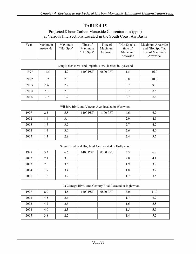
Chapter 4 Revision to the Federal Carbon Monoxide Attainment Demonstration Plan
V-4-33
TABLE 4-15 Projected 8-hour Carbon Monoxide Concentrations (ppm)
at Various Intersections Located in the South Coast Air Basin
Year Maximum Areawide
Maximum "Hot Spot"
Time of Maximum "Hot Spot"
Time of Maximum Areawide
"Hot Spot" at time of
Maximum Areawide
Maximum Areawide and "Hot Spot" at time of Maximum
Areawide
Long Beach Blvd. and Imperial Hwy. located in Lynwood
1997 14.5 4.2 1300 PST 0600 PST 1.5 16.0
2002 9.2 2.3 0.8 10.0
2003 8.6 2.2 0.7 9.3
2004 8.1 2.0 0.7 8.8
2005 7.7 1.9 0.7 8.4
Wilshire Blvd. and Veteran Ave. located in Westwood
1997 2.3 5.8 1400 PST 1100 PST 4.6 6.9
2002 1.6 3.4 2.9 4.5
2003 1.5 3.2 2.7 4.2
2004 1.4 3.0 2.6 4.0
2005 1.3 2.8 2.4 3.7
Sunset Blvd. and Highland Ave. located in Hollywood
1997 3.3 6.6 1400 PST 0300 PST 3.5 6.8
2002 2.1 3.8 2.0 4.1
2003 2.0 3.6 1.9 3.9
2004 1.9 3.4 1.8 3.7
2005 1.8 3.2 1.7 3.5
La Cienega Blvd. And Century Blvd. Located in Inglewood
1997 8.0 4.5 1200 PST 0800 PST 3.0 11.0
2002 4.5 2.6 1.7 6.2
2003 4.2 2.5 1.6 5.8
2004 4.0 2.3 1.5 5.5
2005 3.8 2.2 1.4 5.2

References

California Air Resources Board. 1997a. The 1997 Southern California Ozone Study-NARSTO: Preparation of the 1997 Gridded Emission Inventory. A&WMA June 1998 Presentation California Air Resources Board and the SCOS97-NARSTO Technical Committee. 1998. SCOS97-NARSTO 1997 Southern California Ozone Study and Aerosol Study, Volume III: Summary of Field Operations. April 1998. Douglas S. G. and R. C. Kessler. 1998. “User’s Guide to the Diagnostic Wind Model (Version 1.0).” Systems Applications, Inc. San Rafael, CA. Douglas, S. G., R. C. Kessler, and E. Carr. 1990. “User’s Guide for the Urban Airshed Model. Volume III: User’s Manual for the Diagnostic Wind Model.” EPA Publication No. EPA-450/4-90-007C. U. S. Environmental Protection Agency, Research Triangle Park. NC. ENVIRON, 2002. CAMx User’s Guide Version 3.10. ENVIRON. Novato, CA 94945. April, 2002. Holzworth. G. C. 1967. Mixing depth, wind speeds, and air pollution potential for selected locations in the United States.” J. Appl. Meteor. 6: 1039. Kumar, N.; F. Lurmann, and W.P.L. Carter. 1995. Development of the Flexible Chemical Mechanism Version of the Urban Airshed Model. Final Report STI-94470-1508-FR. PTSD, California Air Resources Board. Sacramento, CA 95814. August 30, 1995. Kumar, N; A. G. Russel, and G. J. McRae, 1992. A Project to add the Carbon-Bond 4 Chemistry to the California Air Resources Board Model (CALGRID). Sigma Research Agreement No. A974-222. PTSD, California Air Resources Board. Sacramento, CA 95814. November, 1992. O’Brien, J. J. 1970. A note on the vertical structure of the eddy exchange coefficient in the planetary boundary layer. J. Atmos. Sci. 27: 1213. Pandis. S. N., Harley R. A.., Cass G. R., and Seinfeld J. H. (1992) Secondary organic aerosol formation and transport. Atmospheric Environment 26A, 2266-2282 SCAQMD. 1994. “Ozone Modeling – Performance Evaluation.” Technical Report V-B. Air Quality Management Plan. South Coast Air Quality Management District. Diamond Bar, CA. 91765. Schere, K. L. and K. L. Demerjian. 1977. “Calculation of Selected Photoyltic Rate Constants over a Diurnal Range.” EPA Publication N. EPA-600/4-77-0115). U. S. Environmental Protection Agency, Research Triangle Park, NC.

Strader R., Lurmann F., and Pandis S. N. (1999) Evaluation of secondary organic aerosol formation in winter. Atmospheric Environment 33, pp 4849-4864. USEPA 1991. Guideline For Regulatory Application of the Urban Airshed Model. EPA Publication No. EPA-450/4-91-013. U.S. Environmental Protection Agency, Research Triangle Park, NC. USEPA 1998b. Use of Models and Other Analyses in Attainment Demonstrations for the 8-Hour Ozone NAAQS (Draft). October 1998. USEPA. 1990. User’s Guide for the Urban Airshed Model. Volume 1: User’s Manual for UAM (CB-IV). OAQPS, USEPA Research Triangle Park, NC. 2771. June 1990. USEPA. 1995. User’s Guide for the CALMET Meteorological Model. EPA-454/B-95-002. Emissions, Monitoring, and Analysis Division. USEPA. Research Triangle Park, NC. 27711. March, 1995. Yamartino, R. J.; J. Scier; S. R. Hana; G. R. Carmichael, and Y. S. Chang. 1989. CALGRID: A Mesoscale Photochemical Grid Model. Volume I: Model Formulation Document Sigma Research Report No. A6-215-74. PTSD, California Air Resources Board, Sacramento, CA 94814. September 1989. Yamartino, R; J. Scire; G. R. Carmichael, and Y. S. Chang. 1992. The CALGRID mesoscale photochemical grid model. Atmospheric Environment 26A: 1493-1512.