filter design, modeling, and the z-plane · laboratory9 july23,2002,releasev3.0 eecs206 laboratory...

Laboratory 9 July 23, 2002, Release v3.0 EECS 206

Laboratory 9

Filter Design, Modeling, and

the z-Plane

9.1 Introduction

So far, we’ve been considering filters as systems that we design and then apply to signalsto achieve a desired affect. However, filtering is also something that occurs everywhere,without the intervention of a human filter designer. At sunset, the light of the sun is filteredby the atmosphere, often yielding a spectacular array of colors. A concert hall filters thesound of an orchestra before it reaches your ear, coloring the sound and adding pleasingeffects like reverberation. Even our own head, shoulders, and ears form a pair of filters thatallows us to localize sounds in space.Quite often, we may wish to recreate these filtering effects so that we can study them

or apply them in different situations. One way to do this is to model these “natural” filtersusing simple discrete-time filters. That is, if we can measure the response of a particularsystem, we would often like to design a filter that has the same (or a similar) response.One of the goals for this laboratory is to introduce the use of discrete-time filters as

models of real-world filters. In particular, we will examine how to apply a modeling approachto understanding vowel signals. This in turn will suggest a way that we might improve theperformance of the vowel classifier we developed in Lab 8 using an automatic modelingmethod.Another goal of this lab is to present a method of filter design called pole-zero placement

design. Working with this method of filter design is extremely useful for building an intuitionof how the z-plane “works” with respect to the frequency domain that you are alreadyfamiliar with. The design interface that we use for this task should help you to develop agraphical understanding of how poles and zeros affect the frequency response of a system.We will use this design methodology both to design a traditional “goal-oriented” lowpassfilter, and to do some filter modeling.

9.1.1 “The Question”

• How can we design filters for certain purposes?

• How can we model vowel production using discrete-time filters?

232 The University of Michigan, All rights reserved

EECS 206 July 23, 2002, Release v3.0 Laboratory 9

9.2 Background

9.2.1 Filters and the z-transform

Previously, we have presented the general time-domain input-output relationship for a causalfilter1 given by the convolution sum:

y[n] = x[n] ∗ h[n] =∑

k

h[k]x[n− k] =∑

k

x[k]h[n− k] , (9.1)

where x[n] is the input signal, y[n] is the output signal, and h[n] is the filter impulse response.Using the z-transform techniques described in Chapter 7 of DSP First, we can also describethe input/output relationship in the z-domain as

Y (z) = H(z)X(z) , (9.2)

where X(z) is the z-transform of x[n], which is the complex-valued function, defined on thecomplex plane2 by

X(z) =∑

n

x[n]z−n , (9.3)

where Y (z) is the z-transform of y[n], defined in a similar fashion, and where H(z) is thesystem function of the filter, which is a complex-valued function defined on the complexplane by one of the following equivalent definitions:

1. The system function is the z-transform of the filter impulse response h[n], i.e

H(z) =∑

n

h[n]z−n . (9.4)

2. For X(z) and Y (z) as defined above, the system function is given by

H(z) =Y (z)

X(z). (9.5)

The system function has a very important relationship to the frequency response of asystem, H(ω̂). The system function evaluated at ejω̂ is equal to the frequency responseevaluated at frequency ω̂. That is,

H(ω̂) = H(ejω̂) . (9.6)

We can derive this result from equation 9.4. If we let z = ejω̂, then we know that H(z) =H(ejω̂) =

∑

n h[n]e−jω̂n. This is simply the definition of a system’s frequency given its

impulse response h[n].

1Note that in this lab, we will only be concerned with causal filters.2The complex plane is simply the set of all complex numbers. The real part of the complex number is

indicated by the x-axis, while the imaginary part is indicated by the y-axis.

The University of Michigan, All rights reserved 233


9.2.2 FIR Filters and the z-transform

For a causal FIR filter, one can easily determine the system function using either of theequivalent definitions given above. However, let us highlight the use of the second definition,which will be useful in the next subsection where the first definition is difficult to apply.In particular, for a causal FIR filter with coefficients {b0, . . . , bM}, the general time-domaininput-output relationship for a causal FIR filter is given by the difference equation

y[n] = b0x[n] + b1x[n− 1] + b2x[n− 2] + · · ·+ bMx[n−M ] . (9.7)

Taking the z-transform of both sides of this difference equation yields

Y (z) = b0X(z) + b1X(z)z−1 + b2X(z)z

−2 + · · ·+ bMX(z)z−M

= X(z)(b0 + b1z−1 + b2z

−2 + b3z−3 + · · ·+ bMz−M ) , (9.8)

where we have used the fact that the z-transform of x[n− no] is X(z)z−no . Dividing both

sides of the above by X(z) gives the system function:

H(z) =Y (z)

X(z)= b0 + b1z

−1 + b2z−2 + b3z

−3 + · · ·+ bMz−M . (9.9)

Notice that H(z) is a polynomial of order M . We can factor the above complex-valuedpolynomial as3

H(z) = K(1− r1z−1)(1− r2z

−1)(1− r3z−1) · · · (1− rMz−1) , (9.10)

where K is a real number called the gain, and {r1, . . . , rM} are the M roots or zeros ofthe polynomial, i.e. the values r such that H(r) = 0. We typically assume that the filtercoefficients bk are real. In this case, the zeros may be real or complex, and if one is complex,then its complex conjugate is also a zero. That is, complex roots come in conjugate pairs.The very important point to observe now from equation (9.10) is that the system function

H(z) of a causal FIR filter is completely determined by its gain and its zeros. Therefore,we can think of {K, r1, . . . , rM} as one more way to describe a filter

4. We will see thatwhen it comes to designing an FIR filter to have a certain desired frequency response, thedescription of the filter in terms of its gain and its zeros is by far the most useful. In otherwords, the best way to design a filter to have a desired frequency response (e.g., a low passfilter) is to appropriately choose its gain and zeros. One may then find the system functionby multiplying out the terms of equation (9.10), and then picking off the filter coefficientsfrom the system function. For example, the number multiplying z−3 in the system functionis the filter coefficient b3. The specific procedure will be described shortly.The fact that we may design the frequency response of a causal FIR filter by choosing

its zeros5 stems from the following principle:

If a filter has a zero r located on the unit circle, i.e. |r| = 1, then H(∠r) = 0,i.e. the frequency response has a null at frequency ∠r. Similarly, if a filter hasa zero r located close to the unit circle, i.e. |r| ≈ 1, then H(∠r) ≈ 0, i.e. thefrequency response has a dip at frequency ∠r. In either case, H(ω̂) ≈ 0, whenω̂ ≈ ∠r.

3The Fundamental Theorem of Algebra guarantees that H(z) factors in this way.4Previous ways of describing a filter have included the filter coefficients, the impulse response sequence,

the frequency response function, and the system function.5The gain does not affect the shape of the frequency response.



The above fact follows from the property that if ω̂ = ∠r and |r| = 1, then ejω̂ = r, and so

H(ω̂) = H(ejω̂) = H(r) = 0 . (9.11)

A similar statement shows H(ω̂) ≈ 0 when |r| ≈ 1 and/or ω̂ ≈ ∠r.From this fact, we see that we see that we can make a filter block a particular frequency,

i.e. create a null or a dip in the frequency response, simply by placing a zero on or near theunit circle at an angle equal to the desired frequency6. On the other hand, the frequencyresponse at frequencies corresponding to angles that are not close to these zeros will havelarge magnitude. The filter will “pass” these frequencies. The specific procedure to designsuch a filter is the following.

1. Choose frequencies ω̂1, ..., ω̂L at which the frequency response should contain a null ora dip.

2. Choose zeros ri = ρiejω̂i , i = 1, . . . , L, with ρi = 1 or ρi ≈ 1, depending upon whether

a null or a dip is desired at frequency ω̂. For each ω̂i 6= 0 choose also a zero rj that isthe complex conjugate of ri. Let M be the total number of zeros chosen.

3. Form the system function H(z) = K(1 − r1z−1) × · · · × (1 − rMz−1), where K is a

gain that we also choose.

4. Cross multiply the factors of H(z) found in the previous step so as to express H(z)as a polynomial whose terms are powers of z−1.

5. Identify the FIR filter coefficients {b0, . . . , bM}, which are simply the coefficients ofthe polynomial found in the previous step, as shown in equation (9.9).

9.2.3 IIR filters and rational system functions

We now consider IIR filters. The general time-domain input-output relationship for a causalIIR filter is given by the difference equation

y[n] = b0x[n] +b1x[n− 1] + b2x[n− 2] + · · ·+ bMx[n−M ]

+a1y[n− 1] + a2y[n− 2] + · · ·+ aNy[n−N ] . (9.12)

Here, we have the usual FIR filter coefficients, bk, but we also have another set of coefficientsak, which multiply past values of the filter’s output. We will call the bk’s the feedforwardcoefficients and the ak’s the feedback coefficients

7. If the ak’s are zero, then this filter reducesto a causal FIR filter.As an example, consider the simple IIR filter with difference equation:

y[n] = x[n] +1

2y[n− 1] (9.13)

What is the impulse response of this filter? If we assume8 that y[n] = 0 for n < 0, one canstraightforwardly show that the impulse response is

h[n] =

(

1

2

)n

, n ≥ 0, (9.14)

6Since non-real zeros must occur in conjugate pairs, we must also place a conjugate zero on the unitcircle, i.e. a zero whose angle is the negative of the first.

7In some texts (and inMatlab), the feedback coefficients are defined as the negatives of the ak coefficientsgiven here. Because of this, you should always be sure to check which convention is used.

8This assumption is one of the “initial rest conditions” discussed in chapter 8 of DSP First.



which is never zero for any positive n. (Note that the impulse response is generally notso simple to compute; this is an unusual case where the impulse response can be obtainedby inspection.) Thus, by introducing feedback terms into our difference equation, we haveproduced a filter with an infinite impulse response, i.e., an IIR filter.In general, computing the system function by taking the z-transform of the resulting

infinite impulse may not be trivial because of the required infinite sum, and also because itmay be difficult to find the impulse response. However, we can use the fact that H(z) =Y (z)/X(z) to determine the system function. To do this, we first collect the y[n] terms onthe left side of the equation and take the z-transform of the result.

y[n]− a1y[n− 1]− · · · − aNy[n−N ] = b0x[n] + b1x[n− 1] + · · ·+ bMx[n−M ]

(9.15)

Y (z)− a1Y (z)z−1 − · · · − aNY (z)z

−N = b0X(z) + b1X(z)z−1 + · · ·+ bMX(z)z−M

(9.16)

Y (z)(1− a1z−1 − · · · − aNz

−N ) = X(z)(b0 + b1z−1 + · · ·+ bMz−M ) (9.17)

H(z) =Y (z)

X(z)=

b0 + b1z−1 + · · ·+ bMz−M

1− a1z−1 − · · · − aNz−N(9.18)

Equation (9.18) shows the general form of the system function of an IIR filters. Since it isthe ratio of two polynomials, it is called a rational function9.Just as we could factor the polynomial in equation (9.9), we can do the same with

equation (9.18) to yield

H(z) = K(1− r1z

−1)(1− r2z−1)(1− r3z

−1) · · · (1− rMz−1)

(1− p1z−1)(1− p2z−2)(1− p3z−1) · · · (1− pNz−1). (9.19)

The roots of the polynomial in the numerator, {r1, . . . , rM}, are again called the zeros ofthe system function. The roots of the polynomial in the denominator, {p1, . . . , pN} arecalled the poles of the system function. K is again a gain factor that determines the overallamplitude of the system’s output. As before, the zeros are complex values where H(z) goesto zero. The poles, on the other hand, are complex values where the denominator goes tozero and thus the system function goes to infinity10. Again, we typically assume that thefilter coefficients bk and ak are real, so both the poles and zeros of the system function mustbe either purely real or must appear in complex conjugate pairs.Just as we could completely characterize an FIR filter by its gain and its zeros, we can

completely characterize an IIR filter by its gain, its zeros, and its poles. As in the FIRcase, this is typically the most useful characterization when designing IIR filters. As before,if the system function has zeros near the unit circle, then the filter magnitude frequencyresponse will be small at frequencies near the angles of these zeros. On the other hand, ifthere are poles near the unit circle, then the magnitude frequency response will be be largeat frequencies near the angles of these poles. With FIR filters we could directly design filtersto have nulls or dips at desired frequencies. Now, with IIR filters, we can design peaks inthe frequency response, as well as nulls. The specific procedure is the following.

1. Choose frequencies ω̂1, ..., ω̂L at which the frequency response should contain a null, adip, or a peak.

9This is a generalization of the terminology that the ratio of two integers is called a rational number.10Technically, because of a division by zero, H(z) is undefined at the location of a pole. However, the

magnitude of the system function becomes very large in the neighborhood of a pole.



2. Choose zeros ri = ρiejω̂i at those frequencies at which a null or a dip should occur,

with ρi = 1 or ρi ≈ 1, as desired. For each such ω̂i 6= 0, choose also a zero rj that isthe complex conjugate of ri. Let M be the total number of zeros chosen.

3. Choose poles pi = ρiejω̂i at those frequencies at which a peak should occur, with

ρi = 1 or ρi ≈ 1 as desired. For each such ω̂i 6= 0 choose also a pole pj that is thecomplex conjugate of pi. Let N be the total number of poles chosen.

4. Form the system function H(z) = K (1−r1z−1)×···×(1−rMz−1)

(1−p1z−1)×···×(1−pNz−1) , where K is a gain that

we also choose.

5. Cross multiply the factors of H(z) found in the previous step and express H(z) as theratio of two polynomials whose terms are powers of z−1.

6. Identify the IIR filter coefficients {a0, . . . , aN , b0, . . . , bM}, which are simply the coef-ficients of the polynomials found in the previous step, as shown in equation (9.18).

Poles and zeros at the origin and at infinity

Here, we have defined our system functions in terms of negative powers of z. This isbecause our general forms for FIR and IIR filters are defined in terms of time delays, andmultiplication of the z-transform of some signal X(z) by z−1 is equivalent to a time delay ofone sample. However, there are may be “hidden” poles and zeros when we express a systemfunction in this matter.Consider first the system function for our FIR filter given by (9.9). If we try to evaluate

this system function at z = 0, we will immediately find that we are dividing by zero. Thus,there is actually a pole at the origin of this system function. To reveal such “hidden” polesand zeros, we express the system function in terms of positive powers of z. To do so, we

multiply by zM

zM, which yields

H(z) =b0z

M + b1zM−1 + b2z

M−2 + b3zM−3 + · · ·+ bM

zM. (9.20)

By the Fundamental Theorem of Algebra, we know that the numerator polynomial has Mroots, and thus the system has M zeros. However, the denominator, zM , has M roots aswell, all at z = 0. This means that our causal FIR system function has M poles at theorigin.In some cases, like the previous example, we find extra poles at the origin. In other

cases, we find extra zeros at the origin. For example, the filter y[n] = y[n − 1] + x[n], hasH(z) = 1

1−z−1 =z

z−1 , from which we see there is one zero at the origin. In still other cases

we find zeros at infinity11. For example, the filter y[n] = x[n − 1], has H(z) = z−1 = 1z ,

from which we see that there is a zero at infinity. In still other cases, we find combinationsof the previous cases. We will call poles and zeros located at the origin or at infinitytrivialpoles and zeros because they do not affect the system’s magnitude frequency response12. Inthis laboratory, we will primarily be concerned with nontrivial poles and zeros (those notat the origin or at infinity).

11A zero at infinity means that |H(z)| → 0 as |z| → ∞. It can be shown that a causal filter can neverhave a pole at infinity.

12Trivial poles and zeros do affect the phase (and thus the delay or time shift) of a system.



−1 −0.5 0 0.5 1

−1

−0.8

−0.6

−0.4

−0.2

0

0.2

0.4

0.6

0.8

1

2

Real Part

Imag

inar

y P

art

Figure 9.1: A pole-zero plot of an IIR filter.

Note that there will always be the same number of poles and zeros in a linear time-invariant system, including both trivial and nontrivial poles and zeros. The total numberequals theM or N , whichever is larger. Such facts are useful for checking to make sure thatyou have accounted for all poles and zeros in a system.

Note also that if one chooses filter coefficients such that the numerator and denominatorcontain an identical factor, i.e. if ri = pj for some i and j, then these factors “cancel” eachother, i.e. the filter is equivalent to a filter whose system function has neither factor.

Pole-zero plots

It is often very useful to graphically display the locations of a system’s poles and zeros. Thestandard method for this is the pole-zero plot. Figure 9.1 shows an example of a pole-zeroplot. This is a two-dimensional plot of the z-plane that shows the unit circle, the real andimaginary axes, and the position of the system’s poles and zeros. Zeros are typically markedwith an ‘o’, while poles are indicated with an ‘x’. Sometimes, a location has multiple polesand zeros. In this case, a number is marked next to that location to indicate how manypoles or zeros exist there. Figure 9.1, for instance, shows four zeros (two conjugate pairs),two “trivial” poles at the origin, and one other conjugate pair of poles. Recall that zerosand poles near the unit circle can be expected to have a strong influence on the magnitudefrequency response of the filter.

9.2.4 Graphical interpretation of the system function

If we take the magnitude of H(z), we can think of |H(z)| as defining a (strictly positive)surface over the z-plane for which the height of the surface is given as a function of thecomplex number z. Figure 9.2 shows an example of just such a surface. This systemfunction has two zeros (which form a complex conjugate pair) and two poles at the origin.Notice that the unit circle is outlined on the surface |H(z)|. The height of the surface atz = ejω̂ (i.e., on the unit circle) defines the magnitude of the frequency response, |H(ω̂)|,which is shown to the right of the surface.



−10

1 −1

0

11

2

3

4

5

Imag(z)Real(z)

(A)

|H(z

)| −1 0 1−1

0

1

2

Real Part

Imag

inar

y P

art

(B)

0 1 2 30

1

2

3

Discrete radian frequency, ω

|H(ω

)|

(C)

Figure 9.2: (A) The z-plane surface defined by the system function H(z) = (1 −ejπ/4z−1)(1 − e−jπ/4z−1). (B) The corresponding pole-zero plot. (C) The correspondingmagnitude frequency response.

−10

1 −1

0

11

2

3

4

Imag(z)Real(z)

(A)

|H(z

)| −1 0 1−1

0

1

2

Real Part

Imag

inar

y P

art

(B)

0 1 2 30

1

2


|H(ω

)|

(C)

Figure 9.3: (A) The z-plane surface defined by the system function H(z) =1

(1−0.8ejπ/2z−1)(1−0.8e−jπ/2z−1). (B) The corresponding pole-zero plot. (C) The corresponding

magnitude frequency response.

−10

1 −1

0

11

2

3

4

Imag(z)Real(z)

(A)

|H(z

)| −1 0 1−1

0

1

Real Part

Imag

inar

y P

art

(B)

0 1 2 30

1

2


|H(ω

)|

(C)

Figure 9.4: (A) The z-plane surface for a complicated system function with four polesand four zeros. (B) The corresponding pole-zero plot. (C) The corresponding magnitudefrequency response.



On Figure 9.2, we can see two points where the surface |H(z)| goes to zero; these are thezeros of the system function. Notice how the surface is “pulled down” in the vicinity of thesezeros, as though it has been “tacked to the ground” at the location of the zeros. Near thesystem’s zeros, the magnitude frequency response has a low point because of the influenceof the nearby zero. Also notice how the surface is “pushed up” at points far from the zeros;this is another common characteristic of system function zeros. (Since the two poles in thisfigure are at the origin, they have no effect on the system’s magnitude frequency response.)Thus, the magnitude frequency response has higher gain at points far away from the zeros.Figure 9.3 shows the surface |H(z)| as defined by a different system function. This

system function has two poles (which form a complex conjugate pair) and two zeros at theorigin. Notice how the poles “push up” the surface near them, like poles under a tent. Thesurface then typically “drapes” down away from the poles, getting lower at points furtherfrom them. The magnitude frequency response here has a point of high gain in the vicinityof the poles. (Again, the zeros in this system function are located at the origin, and thusdo not affect the magnitude frequency response.)Figure 9.4 shows the surface for a system function which has poles and zeros interacting

on the surface. This system function has four poles and four zeros. Notice the tendencyof the poles and zeros to cancel the effects of one another. If a pole and a zero coincideexactly, they will completely cancel. If, however, a pole and a zero are very near one anotherbut do not have exactly the same position, the z-plane surface must decrease in height frominfinity to zero quite rapidly. This behavior allows the design of filters with rapid transitionsbetween high gain and low gain.

9.2.5 Poles and stability

System poles cause the system function to go to infinity at certain values of z because weare dividing by zero. On the one hand, this can have the desirable effect of raising themagnitude frequency response at certain frequencies. On the the other hand, this can havesome undesirable side effects. One somewhat significant problem is introduced if we have apole outside the unit circle. Consider the following filter, for instance:

y[n] = x[n] + 2y[n− 1] (9.21)

This filter has a single pole at z = 2. What is this system’s impulse response? If the inputis x[n] = δ[n] and y[n] = 0 for n < 0, then at n = 0, y[n] = 1. Then, every y[n] after thatis equal to twice the value of y[n − 1]. The value of this impulse response grows as timegoes on! This system is unstable13. Unstable filters cause severe problems, and so we wishto avoid them at all costs. As a general rule of thumb, you can keep your filters from beingunstable by keeping their poles strictly inside the unit circle. Note that the system’s zerosdo not need to be inside the unit to maintain stability.

9.2.6 Filter design using manual pole-zero placement

In this laboratory, we will explore a method of filter design in which we place poles andzeros on the z-plane in order to match some target frequency response. You will be usinga Matlab graphical user interface to do this. The interface allows you to place, delete,

13Technically, it is bounded input, bounded output (BIBO) unstable because the input has a limitedmagnitude but the output does not.



and move poles and zeros around the z-plane. The frequency response will be displayedin another figure and will change dynamically as you move poles and zeros. To keep thefilter’s coefficients real, you will design by placing a pair of poles and zeros on the z-planesimultaneously.The approach for this method depends somewhat on the type of filter that we wish to

design. If we want an FIR filter (i.e., a filter that has no poles), we need to use zeros to“pin down” the frequency response where it is low, and allow the frequency response to bepushed upwards in regions where there are no zeros. Note that if we put a zero right onthe unit circle, we introduce null in the frequency response at that point. Conversely, thecloser to the origin that we place a zero, the less effect it will have on the frequency response(since it will begin to affect all points on the unit circle roughly equally). You might usethe example of the running average filter and bandpass filters (given in Chapter 7 of DSPFirst) as a prototype of how to use zeros to design FIR filters using zero placement.If we wish to design an IIR filter (with both poles and zeros), it usually makes sense to

start with the poles since they typically affect the frequency response to a greater extent.If the frequency response that we are trying to match has peaks on it, this suggests that weshould place a pole somewhere near that peak (inside the unit circle). Then, use zeros totry to pull down the frequency response where it is too high. As with zeros, poles near theorigin have relatively little effect on the system’s filter response.Regardless of which type of filter we are designing, there are a couple of methodological

points that should be mentioned. First, moving a pole or zero affects the frequency responseof the entire system. This means that we cannot simply optimize the position of each pole-pair and zero-pair individually and expect to have a system which is optimized overall.Instead, after adjusting the position of any pole-pair or zero-pair, we generally need to movemany of the remaining pairs to compensate for the changes. This means that filter designusing manual pole-zero placement is fundamentally an iterative design process.Additionally, it is important that you consider the filter’s gain. Often we cannot adjust

the overall magnitude of the frequency response using just poles and zeros. Thus, to matchthe frequency response properly, you may need to adjust the filter’s gain up or down. Thepole-zero design interface that you will use in this Lab includes an edit box where you canchange the gain parameter. Alternately, by dragging the frequency response curve, you canchange the gain graphically. A related idea is that of spectral slope. By having a pair ofpoles or zeros inside the unit circle and near the real axis, we can adjust the overall “tilt”of the frequency response. As we move the pair to the right and left on the z-plane, we canadjust the slope of the system’s frequency response up and down.Note that there are automatic filter design methods which do not require manual place-

ment of poles and zeros. In Section 9.2.8 we discuss one such method.

9.2.7 Design of Standard Filter Types

Many of the filters that we wish to design and use belong to one of four standard types:lowpass, highpass, bandpass, or bandstop. These filters are characterized by a passband (aband of frequencies which are relatively unaltered by the filter) and a stopband (a band offrequencies which are significantly attenuated, or decreased in amplitude, by the filter). Thelocations of the passband and stopband are what characterize the different filter types. Forinstance, a lowpass filter has a passband which contains low frequencies and a stopbandwhich contains high frequencies, while a bandpass filter has a single passband that is sur-rounded by two stopband regions. Between the passband and the stopband is a transition



StopbandPassband

TransitionBand

StopbandAttenuation

PassbandRipple

Frequency

|H(ω

)|

Cutoff Frequency

Figure 9.5: An illustration of the various bands of a lowpass filter.

band in which the filter’s frequency response changes from high to low. The location of thetransition band in frequency determines the filter’s cutoff frequency. In this lab, we willspecify the cutoff frequency by using the two frequencies that bound the transition band.

When designing these types of filter, there are a number of different design goals thatwe may attempt to achieve. For instance, we may wish to have a very flat frequencyresponse in the passband of the filter. Unfortunately, it can be difficult to achieve a flatfrequency response over some frequency region. Instead, the frequency response usuallyvaries somewhat over that region; this variation is called ripple. Thus, one of design criteriamay be to minimize passband ripple. In this lab, we define the passband ripple as the(positive) decibel value of the ratio between the maximum and minimum filter gains in thepassband.

Another common goal is to try to minimize the gain in the stopband of the filter relativeto the gain in the passband. That is, we wish to maximize the stopband attenuation. In thislab, we define the stopband attenuation as the decibel ratio between the maximum filtergain in the passband and the maximum filter gain in the stopband.

Figure 9.5 shows the passband, transition band, and stopband for a lowpass filter. Thefigure also illustrates the the passband ripple and stopband attenuation. In Problem 2 ofthis assignment, you will design a lowpass filter to maximize stopband attenuation.

9.2.8 Modeling Vowel Production

In Lab 8, we discussed some of the properties of vowel production in speech, but we did notexamine the mechanisms behind vowel production. In order to gain a better understandingof vowel production and how we can model it using discrete-time filters, we need to introducesome theory.

Speech production is primarily governed by the larynx (or voice box) and the vocal tract.Figure 9.6 shows a diagram of the larynx and vocal tract. When we speak a vowel, the lungspush a stream of air through the larynx and the vocal folds (commonly referred to as thevocal chords). Given the appropriate muscular tension, this stream of air causes the vocal



Figure 9.6: A diagram showing the larynx and vocal tract.

GlottalSource y[n]Vocal Tract

Filter

x[n]

Figure 9.7: A block diagram of the source-filter model of speech production.

folds to vibrate14. This in turn creates a nearly periodic fluctuation in air pressure passingthrough the larynx. The fundamental frequency of vocal fold vibration is typically around100 Hz for males and 200 Hz for females.

This fluctuating air stream then passes through the vocal tract, which is the airwayleading from the larynx and through the mouth to the lips. The positions of the tongue,lips, and jaw serve to shape the vocal tract, with different positions creating different vowelsounds. The different sounds are produced as the vocal tract shapes the spectrum of thepressure signal coming from the larynx. Depending upon the vocal tract configuration,different frequencies of the spectrum are emphasized; from Lab 8, we know these frequenciesas formants. When whispering a vowel, the lungs push air through the larynx, but the vocalfolds do not vibrate. In this case, the air pressure fluctuation is quite noise-like and generallyis not periodic. Nevertheless, the tongue, lips and jaw shape the vocal tract just as beforeto make the various vowel sounds.

Note that the above description is only accurate for vowels and so-called voiced conso-nants like “m” and “n.” Most consonant sounds are produced using the tongue, lips, andteeth rather than the vocal cords. We will not consider consonants in this lab.

It is traditional to model speech production using a source-filter model. Figure 9.7 showsa block diagram of the source-filter model. The first block is the glottal source, which

14In fact, during normal production the vocal folds open and close completely on each cycle of the vibration.



0 0.5 1 1.5 2 2.5 30

0.5

1

X(ω

)

0 0.5 1 1.5 2 2.5 30

0.5

1

H(ω

)

0 0.5 1 1.5 2 2.5 30

0.5

1

Frequency (radians per sample)

Y(ω

)

Figure 9.8: A plot of the magnitude spectrum of a glottal source signal, the frequencyresponse of a vocal tract filter, and the magnitude spectrum of the output signal.

takes as input a fundamental frequency and produces a periodic signal (the glottal sourcesignal) with the given fundamental frequency. The signal produced is typically modeled asa periodic pulse train. To a first approximation, we can assume that spectrum of this pulsetrain is composed of equal amplitude harmonics. The glottal source signal is meant to beanalogous to the signal formed by the air pressure fluctuations produced by the vibratingvocal cords. Note that to model whispering, the glottal source signal can be modeled usingrandom noise rather than a pulse train.The second block of the source-filter model is the vocal tract filter. This is a discrete-

time filter that mimics the spectrum-shaping properties of the vocal tract. Since we areassuming a source signal with equal-amplitude harmonics, the vocal tract filter providesthe spectral envelope for our output signal. That is, when we filter the source signal withfundamental frequency ω̂0 radians per sample, the k

th harmonic of the output signal willhave an amplitude equal to the filter’s magnitude frequency response evaluated at kω̂0. Thisis illustrated in Figure 9.8 which shows a particular example. The magnitude spectrum ofthe glottal source signal is shown on top, the magnitude frequency response of the vocaltract filter is shown in the center, and the magnitude spectrum of the output signal, whichis the signal that models the specific vowel signal. One may clearly see that, as desired, theenvelope of the spectrum of the vowel signal model matches the spectrum of the vocal tractfilter.In Problem 3 of this assignment, we will make such source-filter models for particular

vowel signals, by measuring the spectrum of the vowel signal and designing an IIR vocaltract filter whose frequency response approximates this spectrum.Typically, our vocal tract filter can have relatively few filter coefficients (i.e., approxi-

mately 10-20 coefficients). Further, the acoustics of the vocal tract suggest that this filtershould be IIR. Often, the vocal tract is modeled using an all-pole filter which has no non-



trivial zeros. This is because an acoustic passageway like the vocal tract primarily affectsa sound through resonances. A resonance is a part of a system that tends to vibrate at acertain resonant frequency, thus amplifying that frequency in signals passed through them.The feedback form of an IIR filter is a direct implementation of resonance; this is how IIRfilters are able to produce high gain at certain frequencies. Using this simple model of speechproduction, it is possible to synthesize artificial vowels.

All-pole analysis and vowel classification

In the last lab, we explored some features for vowel classification that were based on twomeasures of spectral energy in a vowel signal. The development of the source-filter model,however, suggests an acoustically motivated feature for vowel classification. If we assumethat the vocal tract can be modeled with a low-order discrete-time filter, then the vocaltract filter captures all of the relevant information about which vowel has been produced.Variations such as fundamental frequency and type of vowel production (i.e., voiced orwhispered) are restricted to the glottal source and can be neglected. Using samples of thefrequency response of the vocal tract filter as features for vowel classification has been shownto produce good classification results.Fortunately, there are nice mathematical tools for deriving all-pole filter models auto-

matically from a time-domain waveform. These tools, fit the spectrum of a time-domainsignal with poles in a least-squares sense. Note that these tools work directly with the time-domain waveform rather than its spectrum; typically, they return the resulting ak feedbackcoefficients for a filter with those poles, rather than the locations of the poles themselves.We will explore these tools for all-pole analysis in the laboratory assignment, and we willcompare classification performance using features based on these models to the performancewe achieved with our other feature sets from Lab 8.

9.3 Some Matlab commands for this lab

• Calculating the frequency response of IIR Filters: Previously we have usedfreqz to compute the frequency response of FIR filters. We can use the same commandto compute the frequency response of an IIR filter. If our filter is defined by feedforwardcoefficients bk stored in a vector B and feedback coefficients ak stored in a vector A,we compute the frequency response at 256 points using the command:

>> [H,w] = freqz(B,A,256);

As with FIR filters,Matlab’s convention for the bk coefficients is B(1)= b0, B(2)= b1,. . ., B(M+1)= bM . Matlab’s convention for the ak coefficients is A(1)= 1, A(2)= −a1,. . ., A(N+1)= −aN . Both bk and ak are given as defined in equation 9.18. H containsthe frequency response and w contains the corresponding discrete-time frequencies. Al-ternatively, we can compute the frequency response only at a desired set of frequencies.For example, the command

>> [H,w] = freqz(B,A,[pi/4, pi/2, 3*pi/4]);

returns the frequency response of the filter at the frequencies π/4, π/2, and 3π/4.



−1 −0.5 0 0.5 1

−1

−0.8

−0.6

−0.4

−0.2

0

0.2

0.4

0.6

0.8

1

Real(z)

Imag

(z)

2

0 0.5 1 1.5 2 2.5 30.5

1

1.5

2

ω (Discrete radian frequency)

|H(ω

)|

−1−0.5

00.5

1 −1−0.5

00.5

10

1

2

3

Imag(z)Real(z)

|H(z

)|

Figure 9.9: The GUI window for Pole-Zero Place 3-D.

• Pole-Zero Place 3-D: In this laboratory, we will primarily be exploring filter designusing manual pole-zero placement. To help us do this, we will be using a Matlab

graphical user interface (GUI) called Pole-Zero Place 3-D. Pole-Zero Place 3-D allowsyou to place, move, and delete poles and zeros on the z-plane, and provides immediatefeedback by displaying the filter’s frequency response and the |H(z)| surface. Addi-tionally, it calculates some useful statistics for assessing the quality of a particularfilter design.

To run this program you need to download two different files: pole_zero_place3d.mand pole_zero_place3d.fig. To begin Pole-Zero Place 3-D, simply execute15 thecommand

>> pole_zero_place3d;

Once the program starts, the GUI window shown in Figure 9.9 will appear. The axisin the upper left of the window shows a portion of the z-plane with the unit circle.In the lower left is an axis that displays the frequency response of the system. In thelower right is a 3-D axis which displays a 3-D graph of the |H(z)| surface16.

The interface allows you to do a wide variety of things.

1. To add a poles or zeros to the z-plane, click the Add Zeros or Add Poles buttonand then click on the z-plane plot in the upper left of the GUI. The state of thePlace pair checkbox determines whether a single (real) pole or zero is added, orwhether a conjugate pair is added.

15This program was designed to run using Windows systems running Matlab 6 or higher; it will not workwith previous versions of Matlab. It should work with Unix operating systems running Matlab 6, but thishas not been tested.

16This surface plot requires significant computation, and thus it can be toggled on and off using the View

3-D checkbox in the upper right.



Note that the program also adds the hidden poles and zeros that accompanynontrivial poles and zeros. Specifically, for each zero that is added a pole isadded at the origin, or if there is already at least one zero at the origin, insteadof adding a pole at the origin, one zero at the origin is removed, i.e. cancelled.Moreover, for each pole that is added, a zero is added at the origin, or if thereare already poles at the origin, one pole is removed, i.e. cancelled. The systemdoes not allow one to place zeros at infinity, and it can be shown that zeros atinfinity will not be induced by any other choices of poles or zeros.

2. To move a real pole or zero (or a conjugate pair of complex poles or zeros), youmust first select the pole/zero by clicking on one member of the pair. Then, youcan drag it around the z-plane, use the arrow keys to move it, or move it toa particular location by inputting the magnitude and angle (in radians) in theMagnitude and Angle edit boxes.

3. To delete a pole or zero (or pair), select it and hit the Delete Poles/Zeros button.Again, the system will maintain an equal number of poles and zeros by alsoremoving poles or zeros from the origin as necessary. This may also have theeffect of no longer cancelling other poles and zeros, and thus the total number ofpoles and zeros that appear at the origin will change.

4. To change the filter’s gain, you can either use the Filter Gain edit box or youcan click-and-drag the blue frequency response curve in the lower left.

5. To toggle between linear amplitude and decibel displays in the lower two plots,select the desired radio button above the Filter Gain edit box.

6. To rotate the 3-D |H(z)| plot, simply click-and-drag the axes in the lower rightof the GUI. To enable or disable the 3-D plot, toggle the View 3-D checkbox inthe upper right of the GUI

7. To begin with an initial filter configuration defined by the feedforward coefficients,B, and the feedback coefficients, A, start the program with the command

>> pole_zero_place3d(B,A);

This is useful if you wish to start continue working on a design that you hadpreviously saved. You may set either of these parameters to empty ([]) if youdo not wish to specify the filter coefficients.

8. To print the GUI window, you can either use the Copy to Clipboard button tocopy an image of the figure into the clipboard17, or you can print the figure usingthe Print GUI button.

9. To save your current design, use the Export Filter Coefs button. The feedfor-ward and feedback coefficients will be stored in the variables B_pz and A_pz,respectively.

10. To hear your filter’s response to periodic signal with equal-amplitude harmonics,press the Play Sound button. This is particularly useful when using the GUI todesign vocal tract filters for vowel synthesis.

• Pole-Zero Place 3-D – Filter Matching Mode: In “filter matching mode,” youspecify samples of a desired transfer function at harmonically related frequencies and

17Windows operating systems only



try to match that transfer function. The GUI plots a red curve or stem plot alongwith the frequency response function; this is the response we wish to match. Twoedit boxes labeled Linear Matching Error and Decibel Matching Error indicate howclosely your filter matches the desired frequency response. The matching error valuesare computed as the RMS error between the desired frequency response and your filterdesign in both linear amplitude and in decibels.

To start the GUI in this mode, use the following command:

>> pole_zero_place3d(B,A,filter_gains,fund_frq);

filter_gains are the values of the desired filter frequency response at harmonicallyrelated frequencies, and fund_frq is the fundamental frequency (in radians per sam-ple) of the harmonic series at which filter_gains are defined.

• Pole-Zero Place 3-D – Lowpass Design Mode: In “lowpass design mode,” youspecify the maximum frequency of the passband and the minimum frequency of thestopband (both in radians per sample). To start the GUI in this mode, use thefollowing command:

>> pole_zero_place3d(B,A,[pass_max,stop_min]);

In this mode, the GUI computes the passband ripple and the stopband attenuation ofyour lowpass filter design. You can use these measures to evaluate your filter design.The figure in the lower right also displays the passband and stopband of the filter,with appropriate minima and maxima.

• Converting between filter coefficients and zeros-poles: Given a set of filtercoefficients, we often need to determine the set of poles and zeros defined by thosecoefficients. Similarly, we often need to take a set of poles and zeros and compute thecorresponding filter coefficients. There are two Matlab commands that help us dothis. First, if we have our filter coefficients stored in the vectors B and A, we computethe poles and zeros using the commands

>> zeros = roots(B);

>> poles = roots(A);

This is because the system zeros are simply the roots of the numerator polynomialwhose coefficients are the numbers in B, while the system zeros are simply the roots ofthe denominator polynomial whose coefficients are the numbers in A. We can see thisin equation 9.18. To convert back, use the commands

>> B = poly(zeros);

>> A = poly(poles);

Note that we loose the filter’s gain coefficient, K, with both of these conversions.

• Generating pole-zero plots: Frequently, we’d like to use Matlab to make a pole-zero plot for a filter. If our filter is defined by feedforward coefficients B and feedbackcoefficients A (both row vectors), we can generate a pole-zero plot using the command:



>> zplane(B,A);

Alternately, if we have a list of poles, p, and a list of zeros, z, (both column vectors)we can use the following command:

>> zplane(z,p);

An example of a pole-zero plot resulting from this command is shown in Figure 9.1.

• Automatic all-pole modeling: Using the Matlab command aryule, we can com-pute an all-pole filter model for a discrete-time signal. That is aryule automaticallyfinds an all-pole filter whose magnitude frequency response that in some sense matchesthe magnitude frequency response of the signal. If signal is given by signal, the com-mand

>> A = aryule(signal,N);

returns the filter feedback coefficients ak as a vector A. The parameter N indicateshow many poles we wish to use in our filter model. Once we have A, we can computethe filter’s frequency response at 256 points using freqz as

>> [H,w] = freqz(1,A,256);

9.4 Demonstrations in the Lab Section

• The z-transform, system functions, and IIR filters

• The system function “surface,” |H(z)|

• Using Pole-Zero Place 3-D for filter design

• Vocal tract modeling

9.5 Laboratory Assignment

1. (Fit an FIR filter’s frequency response.) Download the files pole_zero_place3d.m,pole_zero_place3d.fig, and lab9_data.mat. In this problem, you will get familiarwith the Pole-Zero Place 3-D program for filter design using pole-zero placement.

In lab9_data, the variable FIR_fr contains samples of the frequency response for asimple FIR filter with six zeros. Execute Pole-Zero Place 3-D using the command

>> pole_zero_place3d([],[],FIR_fr,2*pi/8192);

Use the GUI to find an FIR filter with six nontrivial zeros that matches the frequencyresponse of the original filter. You should be able to get the linear matching error tobe less than 0.1. (Hint: The original filter had all six of its zeros inside the unit circle,so yours should as well.)



• Include the GUI window with your matching filter in your report. In this andthe following problems, make sure that it is possible to read the filter evaluationscores on your printout. (Note: The easiest way to include the GUI windowis to use the Copy to Clipboard button on a Windows machine. After hittingthe button, wait for the GUI to flash white and then paste the result into yourreport.)

• What are the filter coefficients bk and ak for your filter?

• Where are the zeros on the z-plane? Give your answers in rectangular form.

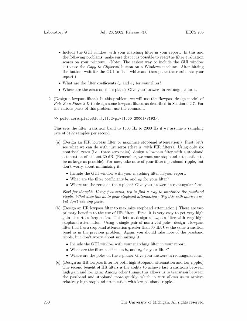
2. (Design a lowpass filter.) In this problem, we will use the “lowpass design mode” ofPole-Zero Place 3-D to design some lowpass filters, as described in Section 9.2.7. Forthe various parts of this problem, use the command

>> pole_zero_place3d([],[],2*pi*[1500 2000]/8192);

This sets the filter transition band to 1500 Hz to 2000 Hz if we assume a samplingrate of 8192 samples per second.

(a) (Design an FIR lowpass filter to maximize stopband attenuation.) First, let’ssee what we can do with just zeros (that is, with FIR filters). Using only sixnontrivial zeros (i.e., three zero pairs), design a lowpass filter with a stopbandattenuation of at least 30 dB. (Remember, we want our stopband attenuation tobe as large as possible). For now, take note of your filter’s passband ripple, butdon’t worry about minimizing it.

• Include the GUI window with your matching filter in your report.


• Where are the zeros on the z-plane? Give your answers in rectangular form.

Food for thought: Using just zeros, try to find a way to minimize the passbandripple. What does this do to your stopband attenuation? Try this with more zeros,but don’t use any poles.

(b) (Design an IIR lowpass filter to maximize stopband attenuation.) There are twoprimary benefits to the use of IIR filters. First, it is very easy to get very highgain at certain frequencies. This lets us design a lowpass filter with very highstopband attenuation. Using a single pair of nontrivial poles, design a lowpassfilter that has a stopband attenuation greater than 60 dB. Use the same transitionband as in the previous problem. Again, you should take note of the passbandripple, but don’t worry about minimizing it.



• Where are the poles on the z-plane? Give your answers in rectangular form.

(c) (Design an IIR lowpass filter for both high stobpand attenuation and low ripple.)The second benefit of IIR filters is the ability to achieve fast transitions betweenhigh gain and low gain. Among other things, this allows us to transition betweenthe passband and stopband more quickly, which in turn allows us to achieverelatively high stopband attenuation with low passband ripple.



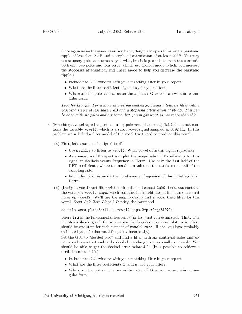
Once again using the same transition band, design a lowpass filter with a passbandripple of less than 2 dB and a stopband attenuation of at least 20dB. You mayuse as many poles and zeros as you wish, but it is possible to meet these criteriawith only two poles and four zeros. (Hint: use decibel mode to help you increasethe stopband attenuation, and linear mode to help you decrease the passbandripple.)



• Where are the poles and zeros on the z-plane? Give your answers in rectan-gular form.

Food for thought: For a more interesting challenge, design a lowpass filter with apassband ripple of less than 1 dB and a stopband attenuation of 60 dB. This canbe done with six poles and six zeros, but you might want to use more than this.

3. (Matching a vowel signal’s spectrum using pole-zero placement.) lab9_data.mat con-tains the variable vowel2, which is a short vowel signal sampled at 8192 Hz. In thisproblem we will find a filter model of the vocal tract used to produce this vowel.

(a) First, let’s examine the signal itself.

• Use soundsc to listen to vowel2. What vowel does this signal represent?

• As a measure of the spectrum, plot the magnitude DFT coefficients for thissignal in decibels versus frequency in Hertz. Use only the first half of theDFT coefficients, where the maximum value on the x-axis is one half of thesampling rate.

• From this plot, estimate the fundamental frequency of the vowel signal inHertz.

(b) (Design a vocal tract filter with both poles and zeros.) lab9_data.mat containsthe variables vowel2_amps, which contains the amplitudes of the harmonics thatmake up vowel2. We’ll use the amplitudes to find a vocal tract filter for thisvowel. Start Pole-Zero Place 3-D using the command

>> pole_zero_place3d([],[],vowel2_amps,2*pi*frq/8192);

where frq is the fundamental frequency (in Hz) that you estimated. (Hint: Thered stems should go all the way across the frequency response plot. Also, thereshould be one stem for each element of vowel2_amps. If not, you have probablyestimated your fundamental frequency incorrectly.)

Set the GUI to “decibel plot” and find a filter with six nontrivial poles and sixnontrivial zeros that makes the decibel matching error as small as possible. Youshould be able to get the decibel error below 4.2. (It is possible to achieve adecibel error of 3.65.)



• Where are the poles and zeros on the z-plane? Give your answers in rectan-gular form.



(c) (Design a vocal tract filter with only poles and zeros.) Now, repeat the above fora filter with 10 poles nontrivial and no nontrivial zeros (except for those at theorigin). You should be able to achieve a decibel matching error below 2.6. (It ispossible to achieve a decibel error of 2.1.)



• Where are the poles on the z-plane? Give your answers in rectangular form.

If you are working on a computer with audio capability, you should use the PlaySound button to listen to a synthesis of the vowel signal. Note that the all-polemodel produces less error with fewer total coefficients. This suggests that all-polefilters are more appropriate for vocal tract modeling.

4. (All-pole modeling and classification) In this problem, we’ll look at an automaticallygenerated all-pole model of vowel2, and we’ll see how we can use this model to helpus improve our vowel classifier performance from Lab 8.

(a) (Automatically generate an all-pole filter model.) Use aryule to compute anall-pole model for vowel2 with 10 poles.

• What are the resulting feedback coefficients?

• Make a pole-zero plot of the resulting filter.

• Use freqz to plot the frequency response of this filter and the frequency re-sponse of the filter you found in Problem 3c in two subplots of the same figure.Display the two frequency responses in decibels. (Note: The two frequencyresponses in decibels may be offset by some constant, which corresponds toa scaling of the original spectrum.)

(b) (Construct and evaluate the vowel classifier.) Here, we’ll consider 16 samplesof the frequency response of an all-pole filter to be a potential feature vector forvowel classification. lab9_data.mat contains five matrices which contain all-polefeature vectors for the same vowel instances we examined in Lab 8. They areoo_ap, oh_ap, ah_ap, ae_ap, and ee_ap.

• As you did in Lab 8, compute the mean all-pole feature vectors for each ofthe five vowel classes. Make sure you label which mean vector belongs withwhich class.

• Combine the above vectors into a matrix of mean feature vectors. Then,use confusion_matrix.m (from Lab 8) to calculate the confusion matrixfor the all-pole features. As you did in Lab 8, use the vowel order “oo,”“oh,” “ah,” “ae,” and “ee”. (Note: if you were unsuccessful at completingconfusion_matrix in Lab 8, you can use the compiled function confusion_matrix_demo.dllfor this problem.)

• Compare this confusion matrix with the two confusion matrices that youcomputed in Lab 8. Is the performance of the classifier better with thisfeature class? Note any similarities between the three confusion matrices.

5. On the front page of your report, please provide an estimate of the average amount oftime spent outside of lab by each member of the group.


filter design, modeling, and the z-plane · laboratory9 july23,2002,releasev3.0 eecs206 laboratory...

Documents