dq-frame modeling of an active power filter integrated

5702 IEEE TRANSACTIONS ON POWER ELECTRONICS, VOL. 28, NO. 12, DECEMBER 2013

DQ-Frame Modeling of an Active Power FilterIntegrated With a Grid-Connected, Multifunctional

Electric Vehicle Charging StationRussell Crosier, Student Member, IEEE, and Shuo Wang, Senior Member, IEEE

Abstract—The paper first proves the existence of a nonlinear,feedback loop due to the effect of an active power filter (APF) on thegrid voltage for a multifunctional electric vehicle charging station.A linear, open-loop model is derived based on direct quadrature(DQ)-theory in discrete time (DT). Based on this model, a linear,closed-loop model is further developed with DQ-theory in DT. Atriangle-hold equivalent instead of a zero-order-hold equivalent isemployed in the model for better representation. The developedlinear, closed-loop model is finally generalized to general powersystems. Simulations are carried out to verify the developed mod-els under transient conditions. The short-time (1–2 ms), transientstability of the grid with an APF is determined with the developedmodel. In contrast to existing stability analyses in the phasor do-main, using DQ-theory can linearize the loop and simplify the loopmodel in DT domain.

Index Terms—Active power filter, direct-quadrature (DQ)-frame, electric vehicle (EV) charging, power system stability,triangle-hold equivalent.

I. INTRODUCTION

W ITH the expected growth of high-tech loads and the in-creasing scrutiny given to voltage quality, active power

filters (APFs) are expected to play an increasingly importantrole in power distribution and delivery [11]. This fact and theavailability of new power electronics technologies have led thefield of APFs to become very diverse in terms of system size andconfiguration [1], [2], [12]. Also, the desire for large pieces ofinfrastructure to serve more than one purpose implies that APFfunctionality will be found in grid interfaces built for a differentprimary purpose. For example, a multifunctional electric vehicle(EV) charging station of multimegawatt capacity is presentedin [12], [16], and [17], and because of its high power level,it was decided that it should be connected directly to mediumvoltage (MV) levels and that it should also provide harmonicand reactive power compensation of the grid current.

By removing reactive and harmonic currents from the grid,APFs improve voltage quality and lower the RMS loadingwhich decreases I2R losses and increases effective capacityand steady-state stability margins. However, with the increasing

Manuscript received October 24, 2012; revised December 22, 2012; acceptedJanuary 19, 2013. Date of current version June 6, 2013. This work was supportedby the National Science Foundation under the award number ECCS-1151126.Recommended for publication by Associate Editor O. C. Onar.

The authors are with the Department of Electrical and Computer Engineer-ing, University of Texas-San Antonio, San Antonio, TX 78249 USA (e-mail:[email protected]; [email protected]).

Digital Object Identifier 10.1109/TPEL.2013.2245515

proliferation of power electronic-based grid interfaces, local-ized, transient stability due to their interaction with the grid isbecoming a general concern.

The EV charging station/APF mentioned earlier is a primeexample of a large APF that could result in grid voltage instabil-ity. Because of its multimegawatt size, it cannot be consideredto be connected to an infinite bus. On the contrary, its outputcurrent will have a significant effect on system voltage (afterall reactive and harmonic compensation is supposed to improvevoltage quality). Because the grid voltage is part of the controlinput for an APF, this introduces a parasitic feedback loop. Forcertain classes of APF [12]–[14], this feedback loop is nonlinearand, thus far, has not been fully analyzed.

Closed-loop, transient instability has been recognized as aconcern for large, grid-connected, equipment [3]. In addition,some points on the grid are highly susceptible to instabilitydue to local resonance [22]. In the past, large APFs, suchas [12], had negligible presence on the grid. Since the pub-lication of [3], the problem of closed-loop stability has beenanalyzed for flexible ac transmission systems (FACTS) such asstatic synchronous compensators (STATCOMs) and static VARcompensators (SVCs) [4]. However, despite the growing sizeand prevalence of APFs, the issue of closed-loop stability hasnot yet been addressed for them in general.

For certain classes of APFs [5], [6], [15], [21] the problem ofstability is much easier to solve. This is because these APFs haveoutput current that is linear, time-invariant (LTI)-related to theother currents and voltages, i.e., they behave like linear elements,allowing a low impedance path for load harmonics. Therefore,these APFs can be integrated into the grid model as just anotherlinear element of the network. However, the functionality ofthese APFs is limited because they cannot identify reactive ornegative-sequence currents (which are nonlinear functions of thegrid voltage), which [12] can do. Therefore, it is desirable thatthe APFs use the grid voltage to identify its reference current.Despite the superior capabilities of APFs in this class, a dynamicmodel for the closed-loop interaction of these APFs with a gridimpedance has not been published.

With the exception of [19], which is the conference paper onwhich this paper is based, the publication most closely related tothis closed-loop issue is [20]. In this paper, the authors considerthe closed-loop interaction of an active, pulse width modulation(PWM)-based rectifier (with dynamic power control based onDQ-theory) with a weak grid. However, the rectifier only drawsactive power, and the additional complexity introduced by APFfunctionality is not considered. Additionally, the grid interaction

0885-8993/$31.00 © 2013 IEEE

Authorized licensed use limited to: University of Florida. Downloaded on December 30,2020 at 05:23:58 UTC from IEEE Xplore. Restrictions apply.

CROSIER AND WANG: DQ-FRAME MODELING OF AN ACTIVE POWER FILTER 5703

Fig. 1. Multifunctional EV charging station in grid compensation mode.(a) Closed-loop system model and (b) reference current identification algorithm.

is only considered for a specific, very simple grid model. Finally,a nonlinear analysis is used, which is in contrast to the analysisherein which transforms the closed loop into an LTI problem.

In this paper and in the conference paper [19] on which this pa-per is based, the nonlinear, closed-loop issue is explained. Then,a procedure is derived to integrate the APF in [12], [16], and [17]into a simple power system and transform the closed-loop modelto a linear framework. This procedure is then generalized. Theequations resulting from this generalization can be applied toany power system and any discrete time (DT)-controlled APFthat can be modeled in the DQ-frame. However, this paper hasthe following additions and improvements: 1), Sections III-Dand IV-B were added in order to model in state-space a loadbeing connected to the system at any time instead of a state-space model based on a load that has always been connected;2), Section V has been completely redone to simulate a systemwith “transient” load in order to verify the math in the newSections III-D and IV-B; 3), Section III-E has been added tojustify certain assumptions that are taken for granted in [19];4), Section V-B has been added to Section V to further justifythose assumptions with simulation; 5), Section VI has beenadded in order to explain the difficulty in attaining experimentalresults for this application at this stage and to propose averification experiment; and finally 6), minor changes beenmade to increase clarity.

II. NONLINEAR, CLOSED LOOP

Fig. 1(a) shows an example of a multifunctional EV chargingstation [12], [16], which is tied to a MV power grid, under APFmode. It will be shown in this section that it results in a nonlinearsystem model. The derivation of this model starts with deriving

the APF’s output current, IC , as a function of Vpcc and Iload ,(1)–(9), and (11). In (11) C(s), the transfer function betweenthe reference and output currents of the APF, is introduced. In(10), Vpcc is written as a function of IC . Then, (10) and (11) arecombined to form the closed-loop model of Vpcc . The closed-loop model is written in its final form in (13).

As shown in Fig. 1(b), the point of common coupling (PCC)voltage is used to identify the active current. First, the instanta-neous power is determined by the dot-product of the three-phasePCC voltage and load current

p(t) = [vpcc,a vpcc,b vpcc,c ]

⎡⎢⎣

iload,a

iload,b

iload,c

⎤⎥⎦ (1)

where p(t) is the instantaneous power of the load.Then, the active power is estimated by passing the determined

instantaneous power through a low-pass filter, F (s)

Pest(s) = L {p(t)} · F (s) (2)

where Pest(s) is the estimated power in the Laplace domain andL{} is the Laplace transform of the instantaneous power from(1). We can also write (2) in the time-domain as

pest(t) =∫ ∞

0p(t − τ) · f(τ)dτ (3)

where f(t) is the time-domain impulse response of the filterF (s). Having estimated the active power, the active currentestimate can be written as [12]⎡

⎢⎣iact,est,a

iact,est,b

iact,est,c

⎤⎥⎦ =

⎡⎢⎣

vpcc,a

vpcc,b

vpcc,c

⎤⎥⎦ pest(t)

v2pcc,a + v2

pcc,b + v2pcc,c

or more compactly as

iact,est,abc = vpcc,abcpest(t)

vTpcc,abc · vpcc,abc

(4)

where iact,est,abc =

⎡⎣

iact,est,aiact,est,biact,est,c

⎤⎦ and vpcc,abc =

⎡⎣

vpcc,a

vpcc,b

vpcc,c

⎤⎦.

Finally, (1), (3), and (4) can be combined to yield

iact,est,abc = vpcc,abc

×∫∞

0 vTpcc,abc(t − τ) · iload,abc(t − τ) · f(τ)dτ


. (5)

Ideally, the compensator should supply all of the undesiredcomponents of the load current iundes in Fig. 1(b), but none ofthe load’s active current iact . Therefore, the reference currentfor the compensator is defined as

iref ,abc = iload,abc − iact,est,abc . (6)

Combining (5) and (6) yields the final expression for thereference current

iref ,abc = iload,abc − vpcc,abc

×∫∞

0 vTpcc,abc(t − τ) · iload,abc(t − τ) · f(τ)dτ


. (7)



Definition (6) makes sense if the load current is separated intoactive and undesired components [as in Fig. 1(b)]. Doing this to(6) yields

iref ,abc = iact,abc + iundes,abc − iact,est,abc . (8)

Since iact,abc − iact,est,abc ≈ 0, (8) can be approximated as

iref ,abc ≈ iundes,abc . (9)

Therefore, definition (6) serves to leave only the undesiredcomponents of the load current (the components that the gridshould not supply) in the reference current of the compensator.The goal of estimating the active current was so that it couldbe removed as accurately as possible from (8). The referencecurrent should only contain iundes,abc because the goal of com-pensation is to remove everything but the active current fromthe grid.

To incorporate the APF into the power system, the PCC volt-age is written as a function of the grid voltage Vg,abc and thecompensator output current based on Fig. 1(a)

Vpcc,abc(s) = Vg,abc(s)ZLoad(s)

ZLoad(s) + ZTh(s)

+ IC,abc(s)ZLoad(s) · ZTh(s)ZLoad(s) + ZTh(s)

where ZTh(s) is the Thevenin impedance of the grid andZLoad(s) is the impedance of the load. This can be simplifiedas

Vpcc,abc(s) =ZLoad(s)

ZLoad(s) + ZTh(s)

× (Vg,abc(s) + IC,abc(s) · ZTh(s)) . (10)

To close the loop, IC,abc(s) needs to be written in terms ofthe other system variables

IC,abc(s) = C(s) · Iref ,abc(s) = C(s) · L{

iload,abc

−vpcc,abc

∫∞0 vT

pcc,abc(t−τ) · iload,abc(t−τ) · f(τ)dτ


}(11)

where L{} is the Laplace transform operator and C(s) is thedynamics of the compensator. Now the loop can be closed bycombining (10) and (11)

Vp cc ,a bc (s) =ZLoad (s)

ZLoad (s) + ZTh (s)

⎛⎝Vg ,a bc (s)

+ C(s) · L

⎧⎨⎩iload ,a bc − vp cc ,a bc

×∫ ∞

0 vTp cc ,a bc (t − τ ) · iload ,a bc (t − τ ) · f (τ )dτ

vTp cc ,a bc · vp cc ,a bc

⎞⎠ · ZTh (s)

⎫⎬⎭.

(12)

Fig. 2. Simple power system incorporating the APF of a multifunctional EVcharging station. (a) Function diagram and (b) DQ-frame equivalent of thereference current.

The final step is to write iload,abc in terms of vpcc,abc . LettingYLoad(s) be the reciprocal of ZLoad(s) in Fig. 1(a), it can be seenthat Iload(s) = Vpcc(s)·YLoad(s) for each phase. This yields thefollowing expression for all three phases in the time domain:

iload,abc(t) =∫ ∞

0vpcc,abc(t − u) · yLoad(u)du.

Substituting this expression into (12) yields (13) as shown atthe bottom of the next page.

Looking inside the L operator in (13), it can be seen thatnonlinear operations occur on vpcc,abc and iload,abc . This is dueto multiplications in (1) and (4). Because these nonlinear oper-ations occur on variables, the L operator will not yield a purelyalgebraic expression. Therefore, the system model is nonlinear,and its stability cannot be analyzed by transfer function methodsalone.

III. DERIVING A LINEAR, CLOSED LOOP

A. Open-Loop System Model

Fig. 2 shows a DT (Z-domain)-controlled APF integrated intoa simple, balanced power system. Before the load is applied (t <τ), the PCC voltage is equal to the grid voltage, vg,abc becausethe line current, iabc , is zero. Letting VG (s) denote the gridvoltage, Vpcc(s) the PCC voltage, IL (s) the load current, IG (s)the grid current, and IC (s) the compensation current injectedto the grid from the APF; the following transfer functions arewritten to model the open-loop system after the switch is closed



(t ≥ τ):⎧⎪⎪⎪⎪⎪⎪⎪⎪⎪⎪⎪⎪⎨⎪⎪⎪⎪⎪⎪⎪⎪⎪⎪⎪⎪⎩

Vpcc(s)VG (s)

=RL + sLL

s (L + LL ) + (R + RL )Vpcc(s)IC (s)

=(R + sL) (RL + sLL )

s (L + LL ) + (R + RL )IL (s)VG (s)

=1

s (L + LL ) + (R + RL )

IL (s)IC (s)

=R + sL

s (L + LL ) + (R + RL ).

(14)

Therefore, using superposition,

Vpcc(s) =RL + sLL

s (L + LL ) + (R + RL )VG (s)

+(R + sL) (RL + sLL )

s (L + LL ) + (R + RL )IC (s)

IL (s) =1

s (L + LL ) + (R + RL )VG (s)

+R + sL

s (L + LL ) + (R + RL )IC (s). (15)

Then according to the procedure given in [10, Sec. 4.4], thiscan be written in the time domain as

d

dt

[x1

x2

]=

[a1 00 a1

] [x1

x2

]+

[a2 a3

a4 1

] [iC

vg

]

[vpcc

iL

]=

[a5 00 a5

] [x1

x2

]+

[a6 a7

a8 0

] [iC

vg

]

+[

a9

0

]d

dt(iC ). (16)

where

a1 =−R − RL

L + LL, a2 = − (RLL − RLL )2

(L + LL )2

a3 =RLL − RLL

L + LL, a4 = −a3

a5 =1

L + LL, a6 =

RL2L + RLL2

(L + LL )2 , a7 =LL

L + LL

a8 =L

L + LL, a9 =

LLL

L + LL

and x1 and x2 are internal variables of the system.In (16), the primary output of interest is vpcc , but the output

iL is also included. This is because iL in the loop of Fig. 2(a)will be closed in Section III-B. Since iC is a function of iL inFig. 2(a), iL is needed to close this loop. However, when the

loop is closed at the end of Section III-B, iL will no longerappear as an output because it is no longer needed.

Since (16) is a per-phase representation of a balanced system,the equation in the ABC-frame is

d

dt

[x1,abc

x2,abc

]=

[(a1)3×3 03×3

03×3 (a1)3×3

][x1,abc

x2,abc

]

+[

(a2)3×3 (a3)3×3

(a4)3×3 I3×3

][iC,abc

vg,abc

]

[vpcc,abc

iL,abc

]=

[(a5)3×3 03×303×3 (a5)3×3

][x1,abc

x2,abc

]

+

[(a6)3×3 (a7)3×3

(a8)3×3 03×3

] [iC,abc

vg,abc

]

+

[(a9)3×3

03×3

]d

dt(iC,abc) (17)

where the notation (u)3×3 indicates a diagonal matrix with u onthe diagonal.

The next step is to transform the system into the DQ0-frame.According to [9], when the following conventions are used

ydq 0 = Tdq 0yabc , yabc = T −1dq 0ydq 0

Tdq 0 =23

×

⎡⎢⎢⎣

cos(ωt + φ) cos(ωt + φ − 120◦) cos(ωt + φ + 120◦)

sin(ωt + φ) sin(ωt + φ − 120◦) sin(ωt + φ + 120◦)

1/2 1/2 1/2

⎤⎥⎥⎦

T −1dq 0 =

⎡⎢⎣

cos(ωt + φ) sin(ωt + φ) 1

cos(ωt + φ − 120◦) sin(ωt + φ − 120◦) 1

cos(ωt + φ + 120◦) sin(ωt + φ + 120◦) 1

⎤⎥⎦ (18)

and φ is defined such that vg,a = Vg cos (ωt + ϕ) (indicatingthat the DQ-frame is aligned to the grid voltage), then the fol-lowing is true:

d

dt(αabc) = (u)3×3 αabc + (v)3×3 βabc

↓

d

dt(αdq0) =

⎡⎢⎣

u −ω 0ω u 00 0 u

⎤⎥⎦αdq0 + (v)3×3

⎡⎢⎣

βd

βq

0

⎤⎥⎦ (19)

where the equation before the arrow represents any first-order, balanced, three-phase system, and βabc is a three-phase-

Vpcc,abc(s) =Zload(s)

Zload(s) + ZTh(s)

(Vg,abc(s) + C(s) ·

(vpcc,abc(s)zLoad(s)

− L ·{

vpcc,abc

·∫∞

0 vTpcc,abc(t − τ) · [

∫∞0 vpcc,abc(t − τ − u) · yLoad(u) · du] · f(τ)dτ


})· ZTh(s)

)(13)



balanced, driving function. Also, in particular

vg,dq0 = Tdq0vg,abc =

⎡⎢⎣

Vg

00

⎤⎥⎦ . (20)

Because β0 is zero in (19), the last line of the DQ0-frameexpression is essentially 0 = 0. Therefore, the DQ-frame can beused instead of the DQ0-frame

d

dt(αabc) = (u)3×3 αabc + (v)3×3 βabc → d

dt(αdq )

=[

u −ω

ω u

]αdq + (v)2×2βdq (21)

where ydq = Tdqyabc , zdq = Tdq zabc , and

Tdq =23

[cos(ωt+φ) cos(ωt+φ−120◦) cos(ωt+φ+120◦)sin(ωt+φ) sin(ωt+φ−120◦) sin(ωt+φ+120◦)

].

Therefore, (21) can be applied to (17) to transform (17) intothe DQ-frame

d

dt

[x1,dq

x2,dq

]= A

[x1,dq

x2,dq

]+ B

[iC,dq

vg,dq

]

[vpcc,dq

iL,dq

]= C

[x1,dq

x2,dq

]+ D

[iC,dq

vg,dq

]+ F

d

dtiC,dq (22)

where

A =

⎡⎢⎢⎣

[a1 −ωω a1

]02×2

02×2

[a1 −ωω a1

]

⎤⎥⎥⎦ , B =

[(a2)2×2 (a3)2×2(a4)2×2 I2×2

]

C =[

(a5)2×2 02×202×2 (a5)2×2

],D =

⎡⎣[

a6 a9ω−a9ω a6

](a7)2×2

(a8)2×2 02×2

⎤⎦

F =[

(a9)2×202×2

].

Also, because

vTdq0idq0 = vT

abcTTdq0Tdq0iabc = vT

abc

23I3x3iabc =

23p (t)

the three-phase, instantaneous power is given by

p (t) =32

(vdid + vq iq + v0i0) =32Vdid . (23)

Equation (23) is true because the DQ-frame is aligned to thegrid voltage, and, therefore, vq and v0 disappear. Hence, poweris proportional to id and is not a function of iq .

For reasons given in Section III-B, the system needs to bemodeled in DT. Therefore, the third step is to transform (22) toDT. To do this, the output variables are redefined by removingthe term F d

dt iC,dq [this term will be restored in (26)][

v′pcc,dq

i′L,dq

]= C

[x1,dq

x2,dq

]+ D

[iC,dq

vg,dq

]. (24)

Fig. 3. Comparison of ZOH and triangle-hold. (a) ZOH and (b) triangle-hold.

Then, the following DT equivalent is applied to (24):

[x1,T H,dq [k + 1]x2,T H,dq [k + 1]

]= Φ

[x1,T H,dq [k]x2,T H,dq [k]

]+ Γ

[iC,dq [k]vg,dq [k]

],

[v′

pcc,dq [k]i′L,dq [k]

]= C

[x1,T H,dq [k + 1]x2,T H,dq [k + 1]

]+ Λ

[iC,dq [k]vg,dq [k]

]

(25)

where Γ = Γ1 + ΦΓ2 − Γ2

⎡⎣

Φ Γ1 Γ204×4 I4×4 I4×404×4 04×4 I4×4

⎤⎦ = e

[A B 04×4

04×4 04×4 ( 1T )4×4

04×4 04×4 04×4

]Ts

Λ = D + CΓ2 , Ts

is the sampling time, and the subscript “TH” has been added tothe state variables x and w to indicate that they are not simplysampled versions of x1,dq and x2,dq .

The aforementioned transformation, (25), is the so-calledtriangle-hold equivalent (also called the noncausal, first-order-hold or the slewer-hold) of (22), and the equations are derivedin [7, Sec. 6.3.2]. The triangle-hold is the DT equivalent of (22)assuming that the quantities vg,dq (t) and iC,abc(t) are piece-wise linear between sampling times [see Fig. 3(b)]. This is incontrast to the more commonly used zero-order-hold (ZOH)equivalent, which assumes that input functions make stepwisetransitions [see Fig. 3(a)]. Step changes in iC,abc(t) would leadto very inaccurate results because the system of Fig. 2(b) ishighly inductive at the PCC. Instead it is assumed that iC,abc(t)transitions linearly between samples. The decision to use thetriangle-hold equivalent is further justified with a discussion inSection III-E and with simulation results in Section V-B.

While this assumption may not be completely accurate forAPFs in general, it is a reasonable assumption for multileveltopologies with a high level count such as [12] and [16]. Thisis because the output current between sampling times has avery low ripple when the number of levels is large enough (seeSection III-E).

The term F ddt iC,dq that was removed for (24) has F ·

(iC,dq [k] − iC,dq [k − 1]) /Ts as its triangle-hold equivalent.Therefore, it can be added back to the output expression of(25) to yield

[vpcc,dq [k]iL,dq [k]

]= C

[x1,T H,dq [k]x2,T H,dq [k]

]+ Λ

[iC,dq [k]vg,dq [k]

]

+F

Ts(iC,dq [k] − iC,dq [k − 1]). (26)



Now (26) and (25) are combined to yield the final, open-loopmodel⎡⎢⎣

x1,T H,dq [k + 1]x2,T H,dq [k + 1]

iC,dq [k]

⎤⎥⎦ = Φ′

⎡⎣

x1,T H,dq [k]x2,T H,dq [k]iC,dq [k − 1]

⎤⎦ + Γ′

[iC,dq [k]vg,dq [k]

]


]= C ′

⎡⎢⎣


⎤⎥⎦+Λ′

[iC,dq [k]vg,dq [k]

](27)

where

Φ′ =[

Φ 04×202×4 02×2

],Γ′=

[Γ

I2×2 02×2

], C ′=

[C − F

Ts

]

Λ′ =(

Λ +[

FTs

04×202×2 02×2

]),

and iC,dq [k] will be derived in the next section.

B. Closed-Loop System Model

To close the loop of Fig. 2, it is first necessary to model theoutput of the APF with respect to the load current. The APFmodeled here will mimic the behavior of the APF in Section II,although it will differ in two ways. The first of these ways isthat the reference current determination and the control will bebased in the DQ-frame, as shown in Fig. 2(a). As shown later,this will allow the nonlinearity of (7) to be avoided. The secondis that it will be controlled in DT. This is because in large APFs(e.g., [12]), it is desirable that the output stage avoid switchinglosses by using a slow switching speed. Therefore, to maximizethe bandwidth of the output current, a deadbeat controller canbe used. Described in [18], this type of control is better forimplementing in DT. Although the details of such a controller aresomewhat complicated, [18] shows that the relationship betweenthe output current and reference current is very simple

[IC,d(z)IC,q (z)

]=

[Iref ,d (z)Iref ,q (z)

]1z

(28)

where IC,dq is the compensator output current in the DQ-frame.Now a DT reference current identification must be derived

that is equivalent to the continuous-time algorithm of (7). Be-cause of (23), instantaneous power flow becomes a function ofonly the variable id . Therefore, real power is proportional tothe average value of id . Therefore, the equivalent of (5) is verysimple in the DQ-frame

IL,d,est(z) = F (z) · IL,d(z) (29)

where F (z) =z(1−e−a T s )

z−e−a T s is a first-order, low-pass filter (LPF)and serves the same purpose as F (s) in Fig. 1(b) and (2).

At this point, it should be noted that the APF is working in thesame DQ-frame as (27) is implying that the APF’s controller hasknowledge of the grid voltage angle. This may not be a realisticassumption. However, this assumption need not be the case, asqualified in the next section, in order for the equations derivedhere to be accurate.

Continuing with the derivation as shown in Fig. 2(b), then,the equivalent of (7) is

Iref ,dq (z) = IL,dq (z) −[

IL,d,est(z)0

]

=

⎡⎣

(z − 1)e−aTs

z − e−aTsIL,d(z)

IL,q (z)

⎤⎦ . (30)

Then, (28) can be combined with (30) to yield

IC,dq (z) =

⎡⎢⎣

(z − 1)e−aTs

z (z − e−aTs )0

01z

⎤⎥⎦ IL,dq (z). (31)

The next step in closing the loop is to write (31) in state-spaceaccording to [7, Sec. 4.2.3]⎡⎢⎣

y1 [k + 1]y2 [k + 1]y3 [k + 1]

⎤⎥⎦ = E · y[k] + H · iL,dq [k], iC,dq [k] = U · y[k]

(32)where

E =

⎡⎣

e−aTs 0 01 0 00 0 0

⎤⎦ ,H =

⎡⎣

1 00 00 1

⎤⎦

and

U =[

e−aTs −e−aTs 00 0 1

].

To close the loop, (32) will be combined with (27), the open-loop system. First, however, substitutions are made for the vari-able iC,dq in (27) and iL,dq in (32) since they will not be drivingfunctions of the closed-loop system

⎡⎢⎣

x1,T H,dq [k + 1]x2,T H,dq [k + 1]

iC,dq [k]

⎤⎥⎦ = Φ′

⎡⎢⎣


⎤⎥⎦

+[Γ′

left Γ′right

] [U · y[k]vg,dq [k]

]


]=

[C ′

1

C ′2

]⎡⎢⎣

xT H,dq [k]wT H,dq [k]

iC,dq [k − 1]

⎤⎥⎦

+

[Λ′

1 Λ′3

Λ′2 Λ′

4

] [U · y[k]vg,dq [k]

]

y[k + 1] = E · y[k] + H

×

⎛⎜⎝C ′

2

⎡⎢⎣


⎤⎥⎦ +

(Λ′

2 Λ′4)[

U · y[k]vg,dq [k]

]⎞⎟⎠

iC,dq [k] = U · y[k] (33)



where [ Γ′left Γ′

right ] = Γ′,

[C ′

1C ′

2

]= C ′,

[Λ′

1 Λ′3

Λ′2 Λ′

4

]=

Λ′.Now the two equations can be combined

⎡⎢⎣

x1,T H,dq [k + 1]x2,T H,dq [k + 1]

iC,dq [k]y [k + 1]

⎤⎥⎦ =

[Φ′ Γ′

leftUHC ′

2 E + HΛ′2U

]⎡⎢⎣


y [k]

⎤⎥⎦

+[

Γ′right

HΛ′4

]vg,dq [k]

vpcc,dq [k] = [C ′1 Λ′

1U ]

⎡⎢⎣


y [k]

⎤⎥⎦

+ Λ′3vg,dq [k] (34)

where the output iL,dq no longer appears as mentioned after(16).

Therefore, after the switch in Fig. 2 closes, the poles of thesystem are the eigenvalues of [ Φ ′ Γ ′

l e f t UH C ′

2 E + H Λ ′2 U ].

It should be noted that in (18) φ is aligned with the gridvoltage instead of the PCC voltage as is the normal case. It wasthis key convention that ultimately led to the derivation of anLTI, state-space model because it led to the reference currentin (30) being a linear function of the load current. This differsfrom (7) where the reference current is a nonlinear function ofthe load current.

C. Remark on the Grid Voltage Reference

In an actual power system, a knowledge of the angle andmagnitude of vg,dq may not be available for the DQ-frame con-troller. Moreover, vg,dq may not be constant due to the actionof automatic generator control (AGC). Furthermore, referringthe DQ-controller’s reference angle to the grid voltage wouldlead to nonzero real current being injected at the PCC at steadystate (because the distinction between real and reactive cur-rent is dependent on the angle of Vpcc). Therefore, in a practi-cal implementation of Fig. 2, the reference angle used by theDQ-controller will converge on the true angle of the PCC volt-age at steady state.

The fact that the DQ-frame’s reference angle is not actuallystationary does not affect the accuracy of (34) for modelingthe rapid transient dynamics as long as the reference angle ofthe controller is stationary during the transient. In real systems,this should be the case because the reference phase for theDQ-controller should not be sensitive to instantaneous phe-nomenon such as voltage flicker and harmonics. Therefore, theD and Q components of the grid voltage will remain stationaryduring the transient.

D. Initial Conditions and Transient Response

In order to use (34) to model the response of system to theclosing switch in Fig. 2(a), the initial state of the system needs tobe determined at some time after the switch closes. The first stepto do this is to define the time frame of the transient response.

For the purposes of this analysis, k = 0 will be defined as thetime at which the switch closes.

The next step is to determine initial voltages and currents inthe system. Before the switch closes, there will be no current inthe system. Because of the inductors, the load current is zero atthe instant the switch closes. Therefore, the compensator currentwill also be zero

iC,dq [0] =[

00

]iL,dq [0] =

[00

]. (35)

Therefore, at the instant the switch closes, the PCC voltagecan be found by ignoring the resistors and applying voltagedivision across the inductors of Fig. 2(a)

vpcc,dq [0] =LL

L + LL· vg,dq [0] =

LL

L + LL

[Vg

0

](36)

where vg,dq [0] is equal to

[Vg

0

]due to (20).

One time sample after the switch closes (k = 1) the loadcurrent will no longer be zero. However, because of the dead-beat delay of the compensator, the compensator current will notrespond to the nonzero load current until k = 2. Therefore, forthe first two time samples (k = 0 and 1) of the transient re-sponse, the system in Fig. 2(a) is essentially running open loop.Therefore, to model the PCC voltage and load current (duringthis time only!), the system can be modeled as if the switch wasalready closed and the grid voltage was suddenly turned on atk = 0. Therefore, the well-known, ZOH equivalent is applied to(22) while dropping iC,dq as an input[

x1,dq [k + 1]x2,dq [k + 1]

]= ΦTrans

[x1,dq [k]x2,dq [k]

]+ ΓTrans

[Vg

0

]


]= CTrans

[x1,dq [k]x2,dq [k]

]+ ΛTrans

[Vg

0

](37)

where k = 0 or 1, ΦTrans = eATs ,ΓTrans = A−1

(ΦTrans − I)[ (a3 )2 x 2I2 x 2

], CTrans = C,ΛTrans = [ (a7 )2 x 2I2 x 2

], and

[ x1 , d q [0]x2 , d q [0] ] = (0)4x1 .

The next step is to solve (26) for the initial states of

[x1,T H,dq

x2,T H,dq]. However, due to the nature of the triangle-hold

[which was used to derive (26)], (26) does not become valid un-til the time sample after the switch closes. Therefore, the initialstate of the system will be taken for k = 1. Then, according to(26)

[x1,T H,dq [1]x2,T H,dq [1]

]= C−1

⎛⎜⎝[

vpcc,dq [1]iL,dq [1]

]− Λ

⎡⎢⎣

00Vg

0

⎤⎥⎦

⎞⎟⎠ . (38)

The final step in determining the initial state is to determinethe state of the vector y[1]. To do this, it is again noted that theload current, iL,dq [k], is zero at and prior to k = 0. This factand the fact that the poles of (32) (eigenvalues of E) are stablemean that the vector y has to be zero at k = 1

⎡⎣

y1 [1]y2 [1]y3 [1]

⎤⎦ =

⎡⎣

000

⎤⎦ . (39)



Fig. 4. (a) Simplified illustration of the voltage-source-inverter (VSI)-basedcurrent source for each phase of the APF, (b) illustration of how vi controlsiC when the VSI is three-level, and (c) illustration of how vi controls iC for a25-level VSI.

Equations (35), (38), and (39) can now be combined to yieldthe initial state:⎡⎢⎢⎢⎢⎢⎢⎢⎢⎢⎢⎢⎣

x1,T H,d [1]x1,T H,q [1]x2,T H,d [1]x2,T H,q [1]

iC,d [0]iC,q [0]y1 [1]y2 [1]y3 [1]

⎤⎥⎥⎥⎥⎥⎥⎥⎥⎥⎥⎥⎦

=

⎡⎢⎢⎢⎢⎢⎢⎢⎢⎢⎢⎣

C−1

⎛⎜⎝[

vpcc,dq [1]iL,dq [1]

]− Λ

⎡⎢⎣

00Vg

0

⎤⎥⎦

⎞⎟⎠

00000

⎤⎥⎥⎥⎥⎥⎥⎥⎥⎥⎥⎦

.

(40)where vpcc,dq and iL,dq at k = 1 are given by (37).

However, this means that (34) cannot be used to calculate theresponse of vpcc,dq at k = 0. That is fine because vpcc,dq [0] isgiven by (36).

E. Discussion of Appropriate Hold

In order to derive a DT equivalent of the system in Fig. 2(a)with respect to iC as an input, it necessary to make some assump-tions about the continuous-time (CT) trajectory of iC betweensampling times. In order to do this, it is necessary to considerhow the current is synthesized. This is illustrated in Fig. 4.

In Fig. 4(a), iC flows from the inverter through an inductor tothe PCC of the grid. The inverter voltage, vi , works with the PCCvoltage (which is assumed to be an infinite bus and constant overa time sample for the purposes of current control) to control thevoltage across the inductor, vL , so that iC is controlled correctly.In the case of a conventional inverter, three-level pulse-width-modulation is used to control the average value of vL over eachtime sample so that iC will transition from iC [k] to iC [k+1],as shown in Fig. 4(b) [the third voltage level is not shown inFig. 4(b) because it is negative Vmax ]. In order to achieve thedeadbeat control of (28), iC [k+1] is set equal iref [k] and vi [k]is calculated accordingly.

For reasons given in [12] and [16], it is unlikely that a three-level inverter will be used for the charging station/APF. Rather,it is likely that a DT-controlled, multilevel inverter with a highlevel count (hereafter referred to as a “next-generation grid in-terface”) will be used. Illustrated in Fig. 4(c) for a 25-levelinverter (only 13 voltage level choices are shown because the

Fig. 5. Generalized APF integrated into a generalized power system.

remaining levels are negative), the control of iC is very similarin principle to the three-level case, except that multilevel PWMis used. As shown in Fig. 4(c), this means that vi and, therefore,vL are more nearly constant over the sample time. Therefore,the slope of iC is nearly constant as it transitions from iC [k] tothe reference current(iC [k+1] = iref [k]) one sample time later.

Obviously, a ZOH would be a poor way to model the CTtransitions of the current between sampling times because thecurrent does not have step changes. Additionally, for iC as aninput to the network in Fig. 2(a), a ZOH equivalent would bemathematically meaningless because of the inductors L andLL . Because there are no step changes in iC and because thereis a delay between iC and iref , a natural choice to model icis a ZOH followed by the smoothing filter 1/Ts

s+1/Ts, which is

chosen because it has a group delay of Ts for low frequencies.However, this approach, which will be referred to as ZOH+LPF,leads to iC changing slope over the course of each sample time.Furthermore, due to the changing slope, the current iC willnot fully transition to the reference current by the end of thesampling time (demonstrated with simulation in Section V-B).

It is much more accurate to assume that iC transitions lin-early from iC [k] to iC [k+1] [dotted line in Fig. 4(c)]. This isknown as the triangle-hold. Therefore, the triangle-hold equiv-alent is applied in (24)–(27). It is much more accurate thanusing a ZOH+LPF and is no more complicated [the triangle-hold equivalent yields a six-state model in (27) as would theZOH+LPF approach]. In Section V-B, simulation is used toverify that a unit-delayed, triangle hold is an accurate outputcurrent with respect to the reference current when a next gen-eration grid interface is used. The simulation results will alsoshow that the ZOH+LPF approach is much less accurate.

IV. PROCEDURE AND EQUATIONS IN THE GENERAL CASE

A. Generalized Procedure for Deriving a Linear, Closed Loop

1) Write the state-space description of the open-loop systemin Fig. 5:

x3n×1(t)=J · x3n×1(t)+m∑

x=1

Kx ·vx,abc(t) + Km+1 ·iC,abc(t),

[vpcc,abc(t)iL,abc(t)

]= L · x3n×1(t) +

m∑x=1

Mx · vx,abc(t)

+ Mm+1 · iC,abc(t) + Mm+2 ·(

d

dtiC,abc(t)

). (41)



where x3nx1 (t) is the state column of length 3n (number ofphases times order of system), m is the number of sources inFig. 5, and J,Kx, L, and M are based on knowledge of thesystem. For the simple case in (17), the state variable consistedof x1,abc and x2,abc . According to the nomenclature of thissection, that would correspond to x6×1(t), and n would equal 2.

2) Transform (41) into the DQ-frame according to the pro-cedure discussed in [9, Ch. 3] and referring the angle of theDQ-transform to the angle of the PCC voltage prior to the tran-sient:

xdq (t) = Jdq · xdq (t) + [K1,dq , . . . ,Km+1,dq ]

⎡⎢⎢⎣

v1,dq

...vm,dq

iC,dq

⎤⎥⎥⎦ ,

[vpcc,dq (t)iL,dq (t)

]= Ldq · xdq (t) + [M1,dq , . . . ,Mm+1,dq ]

×

⎡⎢⎢⎣

v1,dq

...vm,dq

iC,dq

⎤⎥⎥⎦ + Mm+2,dq ·

(d

dtiC,dq (t)

)(42)

where Jdq ,K1∼m ,L, and M are constant if (41) represents abalanced system. If this is not the case, this method will still lin-earize the loop, but the parameters Jdq ,Kx, L, and M will be-come functions of time. Therefore, if the system is unbalanced,(41) should be decomposed into symmetrical components inStep 1.

3) Transform (42) into DT using the triangle-hold equivalent[7]:

xT H [k + 1] = Π′ · xT H [k] + [Δ′1 , . . . ,Δ

′m+1]

⎡⎢⎢⎣

v1,dq

...vm,dq

iC,dq

⎤⎥⎥⎦


]= L′

d q· xT H [k] + [Ω′

1 , . . . ,Ω′m+1]

⎡⎢⎢⎣

v1,dq

...vm,dq

iC,dq

⎤⎥⎥⎦

(43)

where

Π′=[

Π 02n×202×2n 02×2

],Δ1∼m =

[Γ1∼m,1 +Π · Γ1∼m,2−Γ1∼m,2

02×2

]

Δ′m+1 =

[Γm+1,1 + Π · Γm+ ,2 − Γm+1,2

I2×2

],

⎡⎣

Π Γx,1 Γx,2[0] I I[0] [0] I

⎤⎦

= e

⎡⎣

Jd q Kx [0][0] [0] [1/Ts ][0] [0] [0]

⎤⎦ ·Ts

, L′dq = [Ldq ,−Mm+2,dq ],Ω′

1∼m

= M1∼m,dq + LdqΓ1∼m,2 ,Ω′m+1

= Mm+2,dq + Mm+1,dq + LdqΓm+1,2

and Ts is the sampling time.

4) Derive the state-space relationship of iL,dq and iC,dq ac-cording to the APF in Fig. 5:

w[k + 1] = N · w[k] + P · iL,dq [k], iC,dq [k] = Q · w[k](44)

where N,P , and Q are based on knowledge of the compensator.In (29) the low-pass filter, F (z), and the APF dynamics, C(z),were very specific. This time N,P,Q, and R are left open toallow for a general case APF.

5) Close the loop by combining (43) and (44):

[xT H [k + 1]w[k + 1]

]=

[Π′ Δ′

m+1QPL2 N + PΩ′

2,m+1Q

] [xT H [k]w[k]

]

+[

[ Δ′1 , · · · ,Δ′

m ]P · [ Ω′

2,1 , · · ·Ω′2,m ]

]·

⎡⎢⎣

v1,dq

...vm,dq

⎤⎥⎦

vpcc,dq [k] = [L1 Ω′1,m+1 · Q ]

[xT H [k]w[k]

]

+ [ Ω′1,1 , · · ·Ω′

1,m ]

⎡⎢⎣

V1,dq

...Vm,dq

⎤⎥⎦ (45)

where

[Ω′

1,1 , . . . Ω′1,m+1

Ω′2,1 , . . . Ω′

2,m+1

]= [Ω′

1 , . . . Ω′m+1 ],

[L1L2

]=

L′dq , and the output iL,dq no longer appears as happened in

(34).

B. Initial Conditions in the General Case Transient Response

In the simple case, the length of the output of (26) has thesame length as the number of states. Therefore, (26) can besolved for the state vector because C can be inverted. This isnot usually the case with the generalized approach because (41)can have fewer outputs than states. Therefore, (41) needs to bemodified with a new output vector that is equal in length to thestate vector. Since the three-phase system of (41) has 3n states,there should be n, three-phase, linearly independent quantities(either voltage and/or currents) that are physically observable.The important thing about these quantities is that they provideadditional, linearly independent pieces of information and canbe easily determined after the load transient based on funda-mental network theory. This new output vector, which includesthe outputs already in (41), is called outabc , and modifies (41)

outabc (t) =

⎡⎢⎢⎢⎣

vpcc,abc (t)iL,abc (t)

out3,abc (t):

outn,abc (t)

⎤⎥⎥⎥⎦ = Lmod · x3nx1 (t)

+m∑

x=1

Mmod,x · vx,abc (t)

+ Mmod,m+1 · iC,abc (t) + Mmod,m+2 ·d

dtiC,abc (t) (46)



where Lmod and Mmod contain L and M , respectively, from(41), as well as additional rows to make their row count equalto outabc(t).

In the aforementioned equation, the additional rows addedto form Lmod and Mmod are based on knowledge necessary tocreate the additional observable outputs. Likewise, the outputexpression of (42) is modified

outdq (t) =

⎡⎣

vpcc,dq (t):

outn,dq (t)

⎤⎦ = Lmod,dq · xdq (t)

+ [Mmod,1,dq , . . . ,Mmod,m+2,dq ]

⎡⎢⎢⎢⎢⎢⎢⎢⎣

v1,dq (t):

vm,dq (t)iC,dq (t)d

dtiC,dq (t)

⎤⎥⎥⎥⎥⎥⎥⎥⎦

(47)

where the procedure of [7, Ch. 3] is used to transform Lmod andMmod into Lmod,dq and Mmod,dq .

Then, the final step to derive an analog of (38) for the generalcase is to modify the output expression of (43)

outdq [k] = L′mod,dq · xT H [k] + Ω′

mod

⎡⎣

v1,dq [k]:

iC,dq [k]

⎤⎦

where L′mod,dq = [Lmod,dq , −Mmod,m+2,dq ] and Ω′

mod =[ Mmod, 1∼m,dq + Lmod, dq · Γ1∼m,2 , Mmod,m+2,dq +Mmod,m+1,dq + Lmod,dq · Γm+1,2 ], and to solve for xT H [1]:

xT H [1] = L′−1mod,dq · outdq [1] − Ω′

mod

⎡⎣

v1,dq [1]:

iC,dq [1]

⎤⎦ . (48)

In order for (48) to be used, the state of the compensator atk = 1 must be determined. In this case, it cannot be assumedthat load current is zero prior to the transient because there mayhave already been a load present prior to the transient. However,except in rare cases where the load transient results in a step inload current, the compensator state, w[k], will not be affectedby the load transient until k = 2. This is because, accordingto (44), w[k] is a function of the previous value of the loadcurrent, iL,dq [k–1]. Under these circumstances, iC,dq [1] can becalculated as if the load has not been connected. Therefore, thefinal expression for the initial state is

[xT H [1]w[1]

]=

⎡⎢⎣L′−1

mod,dq ·

⎛⎝outdq [1] − Ω′

mod

⎡⎣

v1,dq [1]:

iC,dq [1]

⎤⎦⎞⎠

w [1]

⎤⎥⎦

(49)where the state of the compensator w[1] and the compensatoroutput iC,dq [1] are determined by assuming that the load has notbeen connected and the chosen observable output states outdq [1]are solved for based on knowledge of the circuit and the chosenstates.

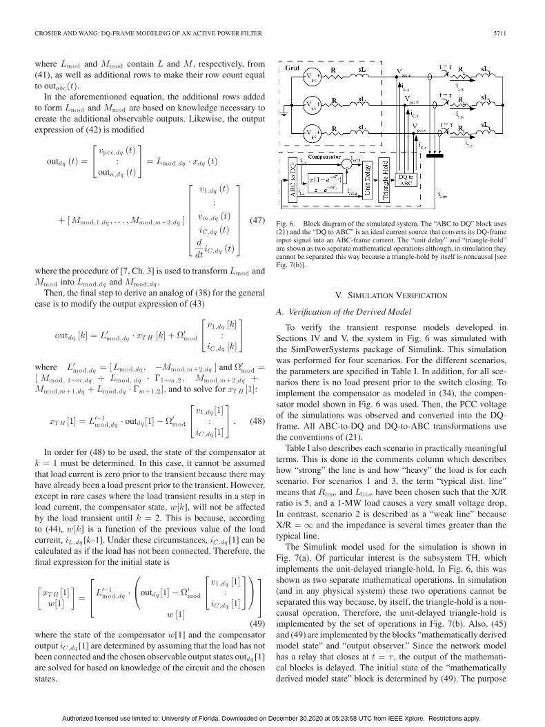
Fig. 6. Block diagram of the simulated system. The “ABC to DQ” block uses(21) and the “DQ to ABC” is an ideal current source that converts its DQ-frameinput signal into an ABC-frame current. The “unit delay” and “triangle-hold”are shown as two separate mathematical operations although, in simulation theycannot be separated this way because a triangle-hold by itself is noncausal [seeFig. 7(b)].

V. SIMULATION VERIFICATION

A. Verification of the Derived Model

To verify the transient response models developed inSections IV and V, the system in Fig. 6 was simulated withthe SimPowerSystems package of Simulink. This simulationwas performed for four scenarios. For the different scenarios,the parameters are specified in Table I. In addition, for all sce-narios there is no load present prior to the switch closing. Toimplement the compensator as modeled in (34), the compen-sator model shown in Fig. 6 was used. Then, the PCC voltageof the simulations was observed and converted into the DQ-frame. All ABC-to-DQ and DQ-to-ABC transformations usethe conventions of (21).

Table I also describes each scenario in practically meaningfulterms. This is done in the comments column which describeshow “strong” the line is and how “heavy” the load is for eachscenario. For scenarios 1 and 3, the term “typical dist. line”means that Rline and Lline have been chosen such that the X/Rratio is 5, and a 1-MW load causes a very small voltage drop.In contrast, scenario 2 is described as a “weak line” becauseX/R = ∞ and the impedance is several times greater than thetypical line.

The Simulink model used for the simulation is shown inFig. 7(a). Of particular interest is the subsystem TH, whichimplements the unit-delayed triangle-hold. In Fig. 6, this wasshown as two separate mathematical operations. In simulation(and in any physical system) these two operations cannot beseparated this way because, by itself, the triangle-hold is a non-causal operation. Therefore, the unit-delayed triangle-hold isimplemented by the set of operations in Fig. 7(b). Also, (45)and (49) are implemented by the blocks “mathematically derivedmodel state” and “output observer.” Since the network modelhas a relay that closes at t = τ , the output of the mathemati-cal blocks is delayed. The initial state of the “mathematicallyderived model state” block is determined by (49). The purpose



TABLE IDESCRIPTION OF THE SIMULATION IN FIG. 7

Fig. 7. (a) Simulink model capture for scenarios 1–4. Of particular interest is the TH block which forces the compensator current to be a unit-delayed, triangle-heldversion of the reference current. (b) TH block model.

of the “to workspace” blocks is to pass the observed simulationand mathematical results to the MATLAB environment so thatFigs. 8 and 9 could be generated.

Each scenario in Table I was also modeled according to (34),the derived closed-loop, DT, DQ-frame model. In accordancewith Section III-D, (36) was used to calculate the PCC voltageat the time of the transient (k = 0). Then, (40) was used to cal-culate the system state at k = 1 in order for (34) to be used forsubsequent values of k. The parameters used for the equationwere based on a sampling rate of 4320 Hz, Vg of 3919 V (the

peak magnitude corresponding to 4800 VRMS,phase-phase), anωg of 2π60/s, and an a [from (29)] of 10/s, and the parametersspecified in Table I. Then, for each scenario, the PCC voltagegenerated by the model is compared to the simulated PCC volt-age in Fig. 9 in the DQ-frame.

Fig. 8 shows the mathematically modeled compensator cur-rent, iC,dq [k], [produced by advancing the state-variable iC,dq [k− 1] in (34)]. Since this is a DT quantity, iC,dq for each valueof k is indicated with an “x.” Since (27) was derived by assum-ing that the continuous compensator current iC,dq (t) is linear



Fig. 8. Mathematically modeled (solid trace) compensator current in the DQ-frame compared to the simulated voltage for the four different scenarios listedin Table I. Note the vertical, gray line in each plot at t = 0.0167 indicates theclosing of the switch in Fig. 2(a).

between sampling times, this was enforced in the simulation.This is also shown in Fig. 8 because the simulated current (solidtrace) connects the DT current with perfectly straight segments.

As Fig. 9 shows, the continuous-time PCC voltage of thephysical model corresponds exactly with the output of the math-ematical model at discrete sampling times. In between samplingtimes, however, the continuous-time voltage may exhibit signif-icant ripple. This is because the triangle-hold assumed for (27)

Fig. 9. Mathematically modeled (solid trace) PCC voltage in the DQ-framecompared to the simulated voltage for the four different scenarios listed inTable I. Since the model is in DT, it perfectly matches the simulated voltage atthe end of each sample time. The vertical, gray line in each plot at t = 0.0167indicates the closing of the switch in Fig. 2(a).

applies only to the inputs of system (which were vg,dq andiC,dq ). It does not imply any nature to the intra-sample trajec-tory of output quantities. If this level of detail in the derivedmodel is required, the reader is referred to [7, Sec. 5.5].

The exact correspondence between simulated and modeledquantities (at sampling times) in Figs. 9 and 10 verifies twothings. The first thing it verifies is the derived procedure to



Fig. 10. Capture of Simulink model to simulate a practical APF. It is similar to the previous simulations except that the effects of a phase-locked loop (PLL), aharmonic load, and a nonideal current source are modeled. The APF and PCC observer blocks measure current and, therefore, have zero throughput impedance.Also, labels have been added for the quantities vi,a bc , iC ,a bc , and vp cc ,a bc to provide context for (50).

TABLE IISIMULATION PARAMETERS

determine the transient response. More importantly, the secondthing it verifies is the correctness of the poles of (34) which canbe used to directly determine stability, stability margins, settlingtime, etc.

B. Verification of Assumptions With a Practical Simulation

The validity of the five-step procedure of Section IV hingeson two very important assumptions regarding the output currentof the APF. The first is that the output current is triangle-heldbetween sampling times. The second is that the output current,iC , is only a function of the load current, iL . This section willvalidate the first assumption. Regarding the second assumption,this section will show that, at sample times, iC is equal to the DTreference current of the previous sample (i.e., deadbeat controlcan be achieved). Therefore, iC can be decoupled from otherstates of the system, validating (44).

Fig. 10 shows a SimPowerSystems model of an APF con-nected to a simple grid with an active, reactive, and harmonicload. In contrast to the previous simulations, this simulation does

not use ideal current sources for the APF. Instead it models thecurrent source for each phase as a cascaded, multilevel inverterin series with an inductor which is how the “next-generation”grid interface will work. The system specifications are given inTable II. Also, the dc-link voltage of the multilevel inverter is333 V and the multilevel PWM is synchronized with the DTcontroller, i.e., there is a 333 V rising or falling edge in eachphase of the inverter voltage every 4320th of a second. Also,DQ-transformations are performed in the reference current, con-troller, and data acquisition blocks according to (21).

To achieve deadbeat control of current, the controller inFig. 10 looks at the difference between output (iC ) and referencecurrents (iref ) at the beginning of each sample and calculatesthe voltage necessary to apply across the inductors, L, in orderto make the error converge to zero at the end of the sample. Thisis done in accordance with [18], which derives the followingrelationship between iC , vi , and vpcc in the DQ-frame:

d

dt(iC,dq ) =

[0 −ωω 0

]iC,dq +

1L

(vi,dq − vpcc,dq ) (50)



Fig. 11. Output current of compensator, iC , (a) compared to the referencewith unit-delayed triangle-hold and (b) compared to the reference current witha ZOH+LPF.

where

iC,dq = Tdq · iC,abc , vi,dq =Tdq · vi,abc , vpcc,dq =Tdq · vpcc,abc ,

Tdq =[

cos (ωt) cos (ωt − 2π/3) cos (ωt + 2π/3)sin (ωt) sin (ωt − 2π/3) sin (ωt + 2π/3)

].

From this point, [18] shows that the appropriate inverter volt-age to achieve deadbeat control is

vi,dq [k] = vpcc,dq [k] + Γ−1 (Iref [k] − ΦiC,dq [k]) . (51)

where Φ = e

[0 −ωω 0

]Ts

, Γ =

[0 −ωω 0

]−1

(Φ − I) /L, and Ts is

the sampling time.This voltage is then transformed back into the ABC-frame

(inside the controller block) and fed as a three-phase referenceto the multilevel inverter block. The multilevel inverter blockthen synthesizes this voltage using per-phase, multilevel, regularsampled (at 4320 Hz) PWM.

In Fig. 11(a), the D-component of the output current, iC , isshown (gray trace). Section III-E argues that the output current isaccurately modeled by applying a unit-delayed, triangle-hold tothe reference current. Therefore, in the same graph the referencecurrent has been plotted with a unit-delayed triangle-hold (blacktrace). Section III-E also theoretically explains the ZOH+LPHapproach but argues that it is a less accurate model of the outputcurrent. Therefore, this model has been compared to the outputcurrent as well in Fig. 11(b).

The results shown in Fig. 11(a) confirm that iC makes rela-tively linear transitions between sampling times and that it fol-lows the unit-delayed reference current closely. Therefore, whendeadbeat control (51) is used with a “next-generation” topology,it is very reasonable to model iC as a unit-delayed, triangle-held version of the reference current. Therefore, the triangle-hold equivalent is an appropriate way to derive a DT-equivalent.Fig. 11(b), however, shows that applying a ZOH+LPF to the ref-erence current is an inferior model of iC . While the ZOH+LPFmodeled current (black trace) does smoothly approximate the

actual iC (gray trace), the black trace follows the gray tracemuch more closely in Fig. 11(a). In addition, there are ripplesin the ZOH+LPF modeled current (black trace) in Fig. 11(b)that are not in the actual iC . These artifacts are not presentin the triangle-hold model [see Fig. 11(a)]. Therefore, even ifthe input of the ZOH+LPF could be modified so that gray andblack traces matched at sampling times, the ripples would stillbe present. Therefore, assuming that iC can be modeled by ap-plying a ZOH+LPF to the reference current will not lead to anaccurate DT-equivalent.

VI. PROPOSED EXPERIMENT SETUP

Experimental results are not currently available. This is be-cause the research reported herein is part of a multiyear, concept-to-prototype project that has not yet reached the hardware stage.Forthcoming results will be reported in future publications.Thus, only a proposal for experimental verification is made.However, the simulations in the previous section were verythorough for that reason. Four scenarios were simulated, andthe mathematical model yielded by the five-step procedure wasvalidated for each one. Also, a second simulation was performedthat validated the assumption that the compensator current canbe modeled by a delayed triangle-hold. In that second simu-lation, the effects of the multilevel inverter (“next-generation”topology), the effects of grid impedance, the dynamics of anactual phase-locked loop (PLL), and the effects of a harmonicload were all simulated.

For verification purposes, the network and APF in Fig. 10 canbe constructed according to the parameters given in Table II. Forthe multilevel inverter of the APF, the topology of [12] will beused, which consists of 12, cascaded H-bridges per phase. Forthe reference current identification (29) will be used, and (51)will be used to control the current. To modulate the multilevelinverter so that the reference voltage is correctly synthesized,the multilevel space vector PWM approach described in [8] canbe used. The DQ-Frame will be defined in accordance with(21), circumventing the need for the PLL block. Finally, theharmonic load (Universal Bridge/Series RLC Load in Fig. 10)will be realized with an independent current source (using thesame topology as the APF).

VII. CONCLUSION

This paper examines a nonlinear, closed loop that is cre-ated when grid-connected power electronics using instanta-neous power-based controllers interact with the grid’s Theveninimpedance ZTh (Fig. 1). This is of particular concern becausethe presence of such devices is expected to increase in the formof large EV charging stations, APFs, distributed generation, dis-tributed storage, etc. In the case of APFs, additional, closed-loopdynamics are introduced that are rapid in nature. The nonlinear,closed loop makes it very difficult to analyze these dynam-ics and, prior to the publication of the conference paper [19] onwhich this paper is based, no suitable method had been publishedto determine the stability, settling time, etc. of these dynamics.

The first contribution of this paper is that it transforms thenonlinear, closed loop into an LTI, closed loop. It uses DQ-theory to do this. This is first done for a simple, DT-controlled



APF connected to a simple power system, yielding a set ofLTI difference equations whose stability and transient responsecan easily be determined. This method is then generalized as astraightforward procedure that yields LTI difference equationsfor a general class of DT-controlled APFs. Furthermore, theprocedure can be easily applied to a wide variety of APFs (anyAPF whose output current is an LTI function of the load cur-rent) connected to any power system that can be modeled asan admittance network. It is finally validated in Simulink for asimple scenario.

This paper does not indicate how to achieve or improve thestability of a grid-connected APF if the closed-loop transientresponse or poles [characteristic values of (34) and (45)] are notfound to be suitably stable. It only provides a straight-forwardway in which to derive an LTI model for a given closed loop.However, it is the authors’ intention that this will provide aframework in which design choices can be made to improvestability and transient response. In particular, there is a lot ofdesign flexibility in the algorithms used by an online controllerto identify the reference current and to make the output currentfollow it. In order to allow the five-step procedure to be veryaccommodating of such design choices, step four of the mod-eling procedure is very open in terms of compensator designdecisions.

The second contribution of this paper is its novel use of thetriangle-hold to model the output current of “next-generation”(as described in Section III-E) grid interfaces. The triangle-hold equivalent was used so that an accurate DT-equivalentcould be derived for the fourth step of the aforementioned, five-step procedure. However, modeling the output current of a nextgeneration grid interface with a triangle-hold has applicationsbeyond modeling a grid-connected APF. Grid interaction can bemore accurately modeled in DT in other medium-voltage, high-power applications such as distributed generation, STATCOMsbecause, as shown in Sections III-E and V-B, a wide variety ofnext-generation grid interfaces will have output current that iswell modeled by the triangle-hold.

REFERENCES

[1] W. Shireen and L. Tao, “A DSP-based active power filter for low voltagedistribution systems,” Electr. Power Syst. Res., vol. 78, pp. 1561–1567,Sep. 2008.

[2] V. Khadkikar, “Enhancing electric power quality using UPQC: A compre-hensive overview,” IEEE Trans. Power Electron., vol. 27, no. 5, pp. 2284–2297, May 2012.

[3] P. Kundur, J. Paserba, V. Ajjarapu, G. Andersson, A. Bose, C. Canizares,N. Hatziargyriou, D. Hill, A. Stankovic, C. Taylor, T. Van Cutsem,and V. Vittal, “Definition and classification of power system stabilityIEEE/CIGRE joint task force on stability terms and definitions,” IEEETrans. Power Syst., vol. 19, no. 3, pp. 1387–1401, Aug. 2004.

[4] A. Ghosh and D. Chatterjee, “Transient stability assessment of powersystems containing series and shunt compensators,” IEEE Trans. PowerSyst., vol. 22, no. 3, pp. 1210–1220, Aug. 2007.

[5] H. Fujita and H. Akagi, “Voltage-regulation performance of a shunt activefilter intended for installation on a power distribution system,” IEEE Trans.Power Electron., vol. 22, no. 3, pp. 1046–1053, May 2007.

[6] D. Basic, V. Ramsden, and P. Muttik, “Harmonic filtering of high-power12-pulse rectifier loads with a selective hybrid filter system,” IEEE Trans.Ind. Electron., vol. 48, no. 6, pp. 1118–1127, Dec. 2001.

[7] G. Franklin, J. Powell, and M. Workman, Digital Control of Dynamic Sys-tems, 3rd ed. Meno Park, CA, USA: Addison-Wesley/Longman, 1998.

[8] D. Holmes and T. Lipo, Pulse Width Modulation for Power Converters:Principles and Practice. Piscataway, NJ, USA: Wiley/IEEE Press, 2003.

[9] P. Krause, O. Wasynczuk, and S. Sudhoff, Analysis of Electric Machineryand Drive Systems. Piscataway, NJ, USA: Wiley/IEEE Press, 2002.

[10] C. Chen, Linear System Theory and Design, 3rd ed. New York, USA:Oxford Univ. Press, 1999.

[11] H. Kanaan, S. Georges, N. Mendalek, A. Hayek, and K. Al-Haddad, “Alinear decoupling control for a PWM three-phase four-wire shunt activepower filter,” in Proc. IEEE Mediterranean Electrotechnical Conf., 2008,pp. 610–618.

[12] R. Crosier and S. Wang, “A 4800-V grid-connected electric vehicle charg-ing station that provides STACOM-APF functions with a bi-directional,multi-level, cascaded converter,” in Proc. IEEE Appl. Power Electron.Conf. Exposition, 2012, pp. 1508–1515.

[13] L. da Silva, L. de Lacerda de Oliveira, V. da Silva, G. Torres, E. Bonaldi,and R. Rossi, “Speeding-up dynamic response of active power condition-ers,” in Proc. IEEE Canadian Conf. Electr. Comput. Eng., 2003, pp. 347–350.

[14] V. Soares, P. Verdelho, and G. Marques, “Active power filter control circuitbased on the instantaneous active and reactive current id –iq method,” inProc. IEEE Power Electron. Specialist Conf., 1997, pp. 1096–1101.

[15] L. Haichun, X. Lizhi, and X. Shaojun, “A method for detecting funda-mental current based on 2nd order series resonant filter,” in Proc. IEEEInt. Power Electron. Motion Conf., 2009, pp. 2411–2415.

[16] S. Wang, R. Crosier, and Y. Chu, “Investigating the power architecturesand circuit topologies for megawatt superfast electric vehicle chargingstations with enhanced grid support functionality,” in Proc. IEEE Int.Electric Vehicle Conf., 2012, pp. 1–8.

[17] Y. Chu and S. Wang, “Bi-directional isolated DC-DC converters withreactive power loss reduction for electric vehicle and grid support appli-cations,” in Proc. IEEE Transp. Electrification Conf., 2012, pp. 1–6.

[18] T. Kawabata, T. Miyashita, and Y. Yamamoto, “Deadbeat control of threephase PWM inverter,” IEEE Trans. Power Electron., vol. 5, no. 1, pp. 21–28, Jan. 1990.

[19] R. Crosier, S. Wang, and Y. Chu, “Modeling of a grid-connected, multi-functional electric vehicle charging station in active filter mode with DQtheory,” in Proc. IEEE Energy Conversion Congress Exposition, 2012,pp. 3395–3402.

[20] C. Wan, M. Huang, C. Tse, S. Wong, and X. Ruan, “Irreversible instabilityin three-phase voltage-source converter connected to non-ideal power gridwith interacting load,” in Proc. IEEE Energy Congress Exposition, Sep.2012, pp. 1406–1411.

[21] Y. Mohammed, “Mitigation of converter-grid resonance, grid-induced dis-tortion, and parametric instabilities in converter-based distributed gener-ation,” IEEE Trans. Power Electron., vol. 26, no. 3, pp. 983–996, Mar.2011.

[22] T. Lee and S. Hu, “Discrete frequency-tuning active filter to suppressharmonic resonances of closed-loop distribution power systems,” IEEETrans. Power Electron., vol. 26, no. 1, pp. 137–148, Jan. 2011.

Russell Crosier (S’12) received the B.S.E.E andM.S.E.E. degrees from the University of Texas-SanAntonio, San Antonio, TX, USA, in 2006 and 2012,respectively.

From 2006 to 2008, he was with the Department ofEnergy, Montana State University, Bozeman, USA,working on a project in the area of power electron-ics and power factor correction His research interestsinclude stability of grid-connected power electronicsand the control of a multimegawatt, superfast, elec-tric vehicle charging station.

Shuo Wang (S’03–M’06–SM’07) received the Ph.D.degree from Virginia Tech, Blacksburg, UA, USA, in2005.

He has been with the Department of Electricaland Computer Engineering, University of Texas-SanAntonio, San Antonio, USA, since 2010. He haspublished more than 90 journal and conference pa-pers. He holds six U.S. patents and has one morepending.

Dr. Wang received the Best Transaction PaperAward from the IEEE Power Electronics Society in

2006 and two William M. Portnoy Awards from the IEEE Industry ApplicationsSociety in 2004 and 2012, respectively. In March 2012, he received the presti-gious National Science Foundation CAREER Award. He is an Associate Editorfor the IEEE TRANSACTIONS ON INDUSTRY APPLICATIONS.


dq-frame modeling of an active power filter integrated

Documents