
Hong, Y., Wang, L., Zhang, J. and Gao, Z. (2020) 3D elastoplastic model for fine-grained gassy soil considering the gas-dependent yield surface shape and stress-dilatancy. Journal of Engineering Mechanics, 146(5), 04020037. (doi: 10.1061/(asce)em.1943-7889.0001760). This is the author’s final accepted version. There may be differences between this version and the published version. You are advised to consult the publisher’s version if you wish to cite from it.
http://eprints.gla.ac.uk/201469/
Deposited on: 23 October 2019
Enlighten – Research publications by members of the University of Glasgow http://eprints.gla.ac.uk
1
3D elastoplastic model for fine–grained gassy soil considering the gas–dependent 1 yield surface shape and stress–dilatancy 2
Yi Hong, Lizhong Wang*, Jianfeng Zhang and Zhiwei Gao 3
Abstract 4
Fine–grained sediments containing large discrete gas bubbles are widely distributed in 5
the five continents throughout the world. The presence of gas bubbles could either 6
degrade or enhance the hardening behaviour and undrained shear strength (𝑠u) of the 7
soil, depending on the initial pore water pressure (𝑢w0) and initial gas volume fraction 8
(ψ0). The existing constitutive models, however, can solely capture either detrimental 9
or beneficial effect owing to presence of gas. This study presents a new three–10
dimensional 3D elastoplastic constitutive model that describes both damaging and 11
beneficial effects of gas bubbles on the stress–strain behaviour of fine–grained gassy 12
soil in a unified manner. This was achieved by incorporating 1) a versatile expression 13
of yield function that simulates a wide range of yield curve shapes in a unified context, 14
and 2) a dilatancy function capturing the distinct stress–dilatancy behaviour of fine–15
grained gassy soil. Given the lack of direct experimental evidence on the shape of the 16
yield curve of fine–grained gassy soil, new experiments were performed. This has led 17
to the identification of three distinct shapes of bullet, ellipse, and teardrop as well as 18
formulation of the yield function considering the dependency of yield curve shapes on 19
𝑢w0 and ψ0. The new model was shown to reasonably capture both the damaging and 20
beneficial effects of gas on the compression and shear behaviour of three types of fine–21
grained gassy soils with a broad range of 𝑢w0 and ψ0 by using a unified set of 22
parameters. 23

2
Author keywords: Constitutive modeling; Fine–grained gassy soil; Yield surface; 24
Stress dilatancy; Critical state. 25
Introduction 26
Bubbles of undissolved gas, produced either biogenically or thermogenically, are 27
widely present within shallow marine sediments throughout the five continents in the 28
world (Grozic et al. 2000). Unlike the conventional unsaturated soils, the degree of 29
saturation of fine–grained gassy marine sediments usually exceeds 85% (Sparks 1963; 30
Nageswaran 1983), with a continuous water phase but a discontinuous phase of gas in 31
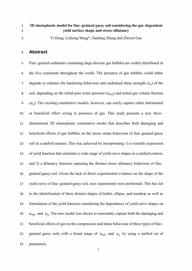
discrete forms, as characterized by Hong et al. (2019a) using a micro–computed 32
tomography (μCT) (Fig. 1(a)). The gas bubbles are significantly larger than the void 33
spaces of the saturated soil matrix as shown in the scanning electron microscopy image 34
in Fig. 1(b); thus, they cannot be treated as occluded bubbles that simply reduce the 35
compressibility of the pore fluid (Wheeler 1988a, 1988b). Consequently, the large gas 36
bubbles should have altered the structure of the soil to dramatically modify the 37
mechanical behaviour of the soil (Wheeler 1988b; Lunne et al. 2001; Hight and 38
Leroueil 2003; Puzrin et al. 2011; Rebata–Landa and Santamarina 2012; Sultan et al. 39
2012), with significant implications on the instability of offshore structures such as 40
monopiles and pipelines and the occurrence of submarine landslides in gassy seabeds 41
(Thomas et al. 2011; Kvenvolden 1988; Nisbet and Piper 1998; Milich 1999; Locat and 42
Lee 2002; Kortekaas and Peuchen 2008; Dittrich et al. 2010; Evan 2011; Rowe and 43
Mabrouk 2012; Xu et al. 2018). 44
The published experimental results (Wheeler 1988b; Hong et al. 2017) have 45
3
suggested that the presence of gas bubbles could either degrade or enhance the 46
hardening behaviour and undrained shear strength (𝑠u) of the soil, depending on the 47
initial pore water pressure (𝑢w0) and initial gas volume fraction (ψ0). On the other hand, 48
the damaging and beneficial effects (𝑠u decreasing or increasing with ψ0, respectively) 49
due to presence of gas had been treated separately by the existing constitutive models 50
for fine-grained gassy soil. Sultan and Garziglia (2014) proposed an anisotropic Cam 51
Clay based constitutive model accounting for the damaging effect by gas. A new 52
analytical expression that relates the preconsolidation pressure to a damage parameter 53
depending on gas content was derived, and coupled to a yield surface considering both 54
inherent and stress-induced anisotropy. The beneficial effect by gas had been 55
considered in the models developed by Pietruszczak and Pande (1996) and Grozic et al. 56
(2005). This is achieved by simplifying the gas bubbles and the pore fluid as a single 57
phase of compressible fluid, which could have beneficially reduced the excess pore 58
water pressure due to undrained shearing, and thus a higher value of 𝑠u . Wheeler 59
(1988b) attempted to approximate the damaging and beneficial effects of gas bubbles 60
on the 𝑠u value of fine–grained gassy soil, by deriving two separate solutions for the 61
upper and lower bound values for 𝑠u. An exact solution for the 𝑠u value for a fine–62
grained gassy soil is still lacking. 63
Despite the afore–mentioned valuable efforts, the lack of a unified framework to 64
capture both damaging and beneficial effects of gas bubbles on the stress–strain 65
relationship (and thus 𝑠u value) of gassy soil has hindered reliable analysis and the 66
design of offshore structures to be built on gassy seabeds. For these reasons, a new 67
4
elastoplastic constitutive model is proposed in this study to simulate the distinct features 68
of fine–grained gassy soil in a unified manner. The new model was formulated to 69
consider the published experimental evidence associated with the compression 70
behaviour (Thomas 1987; Puzrin et al. 2011; Hong et al. 2017), dilatancy (Hong et al. 71
2019b) and critical state (Wheeler 1986; Sham 1989; Hong et al. 2017) as well as the 72
new experiments performed in this study that revealed the versatile the shapes of yield 73
surface of the gassy soil. The predictive capability of the model was validated against 74
the results of three types of fine–grained gassy soils, which cover a broad range of 𝑢w0 75
and ψ0. 76
Key Features of Fine–grained Gassy Soil and Implementations 77
for Constitutive Modeling 78
The behaviour of fine–grained gassy soil has been investigated during the past three 79
decades through experimental work primarily involving oedometer tests and undrained 80
triaxial compression tests. The key features of the fine–grained gassy soil, including the 81
compression and undrained shear behaviour, are reviewed in this section, with 82
particular emphasis on their implications to the elastoplastic modeling of the soil. It is 83
worth noting that this review and the subsequent theoretical development are concerned 84
mainly with the behaviour of gassy soil under in–situ conditions. The behaviour of fine–85
grained gassy soil after significant unloading, such as that owing to deep–water 86
sampling which causes bubble expansion and weakening of the soil structure) has been 87
reviewed and modeled by Sultan and Garziglia (2014), and is beyond the scope of this 88
study. 89
5
Compression behaviour 90
Consolidation tests of fine–grained gassy soils based on oedometer (Thomas 1987; 91
Puzrin et al. 2011) and triaxial apparatus (Hong et al. 2017) suggest that gas bubbles 92
and the saturated matrix contribute independently to the total compressibility. This 93
experimental evidence reveals that although gassy soil becomes more compressible at 94
higher gas content, the compressibility of the saturated matrix is not altered by the 95
volumetric gas content. In particularly, the water void ratio 𝑒w (i.e., the void ratio of 96
the saturated matrix) is a sole function of the effective mean stress. 97
These experimental observations have implied three important aspects for the 98
modeling of fine–grained gassy soil (𝑆r>85%): (Ⅰ) The effective stress principle appears 99
to be valid for describing the behaviour of fine–grained gassy soil; (Ⅱ) a single set of 100
material constants (e.g., 𝜆 and 𝜅 as defined in the Modified Cam–clay (MCC) model) 101
can adequately characterize the compression behaviour of the saturated matrix, 102
irrespective of the gas content; and (Ⅲ) the effective pre–consolidation pressure (𝑝0′ ) 103
of the soil is not altered by the addition of gas. 104
Undrained shear strength 105
A distinct feature of fine–grained gassy soil is that, the presence of gas can either 106
reduce or increase the undrained shear strength 𝑠u of the soil at the same consolidation 107
pressure 𝑝0′ , depending on the initial pore water pressure 𝑢w0 and ψ0 (Wheeler 108
1988b; Hong et al. 2017). Attempts were made to reveal the underlying mechanisms, 109
by analyzing the distributions of the local stress states and local 𝑠u values around the 110
bubbles in soils under different values of initial pore water pressure 𝑢w0 (Wheeler 111
1988a, 1988b; Sham 1989). The analyses were performed on the basis of rigid–112
6
perfectly plastic cavity contraction analysis on a saturated matrix containing a spherical 113
cavity. It was revealed that the presence of gas bubbles led to two completing 114
mechanisms: (Ⅰ) shear failure around the bubble, which reduces the global 𝑠u of the 115
gassy soil, and (Ⅱ) heterogeneity of the saturated matrix (i.e., a denser state of soil near 116
the bubble than that in the far field), which increases the global 𝑠u of the soil. The 117
former (damaging effect) and the latter mechanisms (beneficial effect) were shown to 118
dominate when the value of 𝑢w0 was relatively high and low, respectively. 119
Stress–dilatancy relation 120
Hong et al. (2019b) experimentally revealed that the addition of gas could make the 121
fine–grained soil either more or less contractive, depending on the combination of 𝑢w0 122
and ψ0. These features cannot be captured by the stress–dilatancy function (D) of the 123
modified Cam–clay model. A new function D was thus developed, by introducing a 124
dilatancy multiplier 𝐹 that considers the coupling effects of 𝑢w0 and ψ0 into the 125
dilatancy function of the MCC model, as follows: 126
𝐷 =d𝜀v
p
d𝜀qp = 𝐹 (
𝑢w0 − 𝑢w0_ref
𝑝0′ ,\0)
𝑀2 − 𝜂2
2𝜂
= [1 + 𝜉𝑢w0 − 𝑢w0_ref
𝑝0′ exp (−
𝜒\0
)]𝑀2 − 𝜂2
2𝜂
(1)
where 𝐹(𝑢w0−𝑢w0_ref𝑝0
′ ,\0) denotes the dilatancy multiplier; 𝑢w0_ref denotes the 127
reference 𝑢w0 at which the stress–dilatancy of a gassy soil is similar to its saturated 128
equivalent. 𝜉 and 𝜒 are two material constants for scaling the effects of 𝑢w0 and ψ0 129
on the dilatancy of the gassy soil; and 𝜂 denotes the stress ratio (i.e., 𝜂=𝑞/𝑝′), where 130
the effective mean stress 𝑝′ and deviatoric stress 𝑞 in the triaxial stress space are 131
7
defined as functions of the major (𝜎1′) and minor (𝜎3
′) effective principle stresses, as 132
follows: 133
𝑝′ = (𝜎1′ + 2𝜎3
′) 3⁄ (2)
𝑞 = 𝜎1′ − 𝜎3
′ (3)
where 𝑀 is the stress ratio at the critical state, and 𝑝0′ denotes the initial effective 134
mean stress. The proposed function has been validated against the stress–dilatancy 135
relations from 36 tests (series I and II) on gassy specimens and 1 test on a saturated 136
specimen (Hong et al. 2019b). The new function is shown to effectively capture the 137
following key features related to the stress–dilatancy of fine–grained gassy soil: 138
1. 𝐹 (𝑢w0−𝑢w0_ref𝑝0
′ ,\0) > 1 when 𝑢w0 > 𝑢w0_ref ;and 𝐹 (𝑢w0−𝑢w0_ref𝑝0
′ ,\0) < 1 139
when 𝑢w0 < 𝑢w0_ref. This implies that gassy soil at a relatively high initial pore 140
water pressure (when 𝑢w0 > 𝑢w0_ref) exhibits more contractive response than the 141
saturated soil, and vice versa. 142
2. 𝐹 (𝑢w0−𝑢w0_ref𝑝0
′ ,\0) = 1 when 𝑢w0 = 𝑢w0_ref , and Eq. (1) is equivalent to the 143
dilatancy relation of the MCC model. This means the two competing mechanisms 144
by the presence of gas, as discussed in the preceding sub–section, are cancelled out 145
for this special case, resulting in gassy soil dilatancy equal to that of its saturated 146
equivalent. 147
3. 𝐹 (𝑢w0−𝑢w0_ref𝑝0
′ ,\0) = 1 when ψ0 = 0 (saturated soil), irrespective of the value of 148
𝑢w0. Under this circumstance, Eq. (1) is naturally recovered to the dilatancy relation 149
of the MCC model. 150
4. D = 0 at the critical state (𝑀 = 𝜂). 151
8
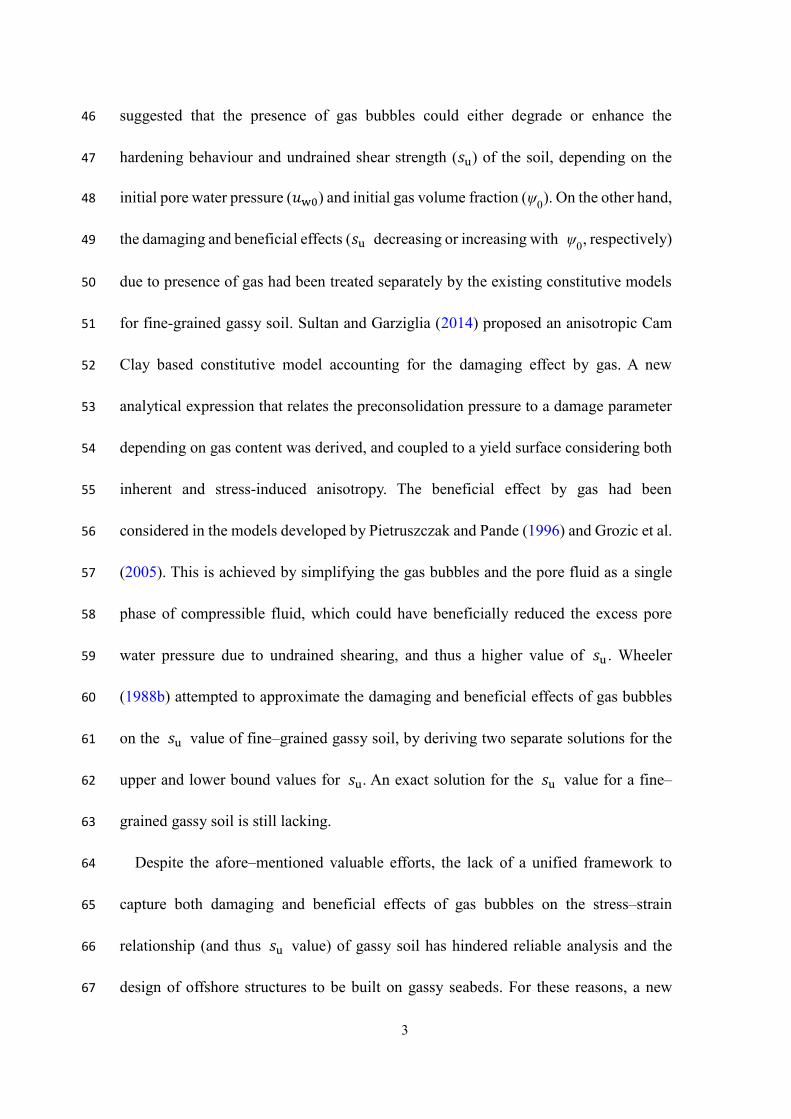
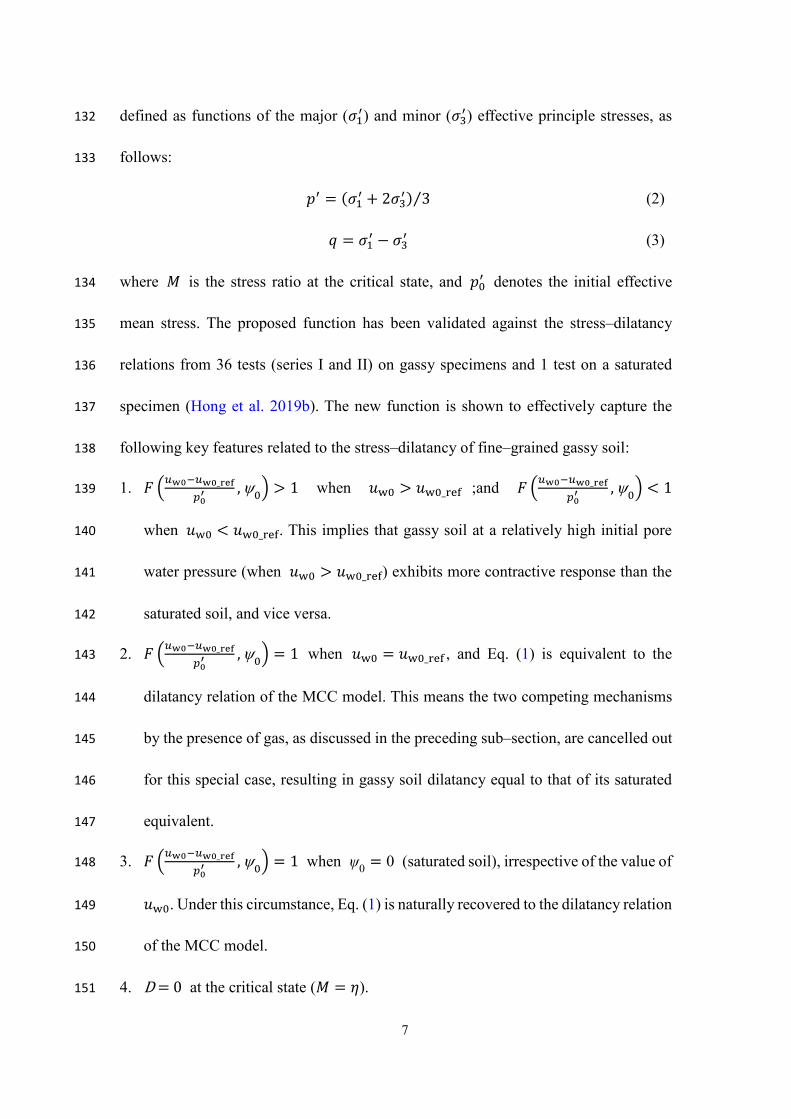
Implied shape of yield curve 152
It is widely accepted that the shape of the yield curve (on the wet side) of a soil can 153
be reflected by the locus of the undrained effective stress path of a normally 154
consolidated specimen. Hong et al. (2019b) reported undrained effective stress paths of 155
normally consolidated gassy Malaysia kaolin silt, which were prepared at the same 156
value of 𝑝0′ , 200 kPa, but under different values of 𝑢w0 at 0, 150, and 600 kPa, as 157
shown in Fig. 2. The loci of these effective stress paths imply that the fine–grained 158
gassy soils exhibit three distinct shapes of yield curves, i.e., teardrop, ellipse and bullet 159
shapes, which occur at relatively low, moderate, and high values of 𝑢w0, respectively. 160
Obviously, these variations in the shape of yield curve cannot be captured by the yield 161
function of the MCC model. The results in Fig. 2 suggest the necessity of introducing 162
a versatile function that considers the three distinct shapes of yield curves with a single 163
set of parameters, in the elastoplastic modeling of gassy soil. In addition to the implied 164
shapes of yield curve via effective stress paths (Fig. 2), new experiments are still desired 165
to explicitly reveal the yield curve shapes, and to formulate the relation between the 166
shape and the state of gassy soil. Details are given in the section titled “Experimental 167
Investigation of Yield Curve and Flow Rule.” 168
Critical state 169
Despite the distinctively different loci of effective stress paths in the 𝑝′ − 𝑞 plane 170
for gassy specimens with varying 𝑢w0 (Fig. 2), their stress ratios at the critical state 171
(i.e., 𝑀) are equal to that of the saturated specimen, irrespective of the gas content 172
(Hong et al. 2017). Moreover, the critical state line (CSL) in the 𝑒w − ln𝑝′ plane 173
remains parallel to the normal consolidation line (Wang et al. 2018), with a slope (i.e., 174
9
𝜆) independent of the gas content. The presence of gas, however, alters the position of 175
the CSL in the 𝑒w − ln𝑝′ plane (Wang et al. 2018) because the gassy soils with the 176
same 𝑒w but different values of 𝑢w0 fail at different 𝑝′, under undrained shearing. 177
A New Constitutive Model for Fine–grained Gassy Soils 178
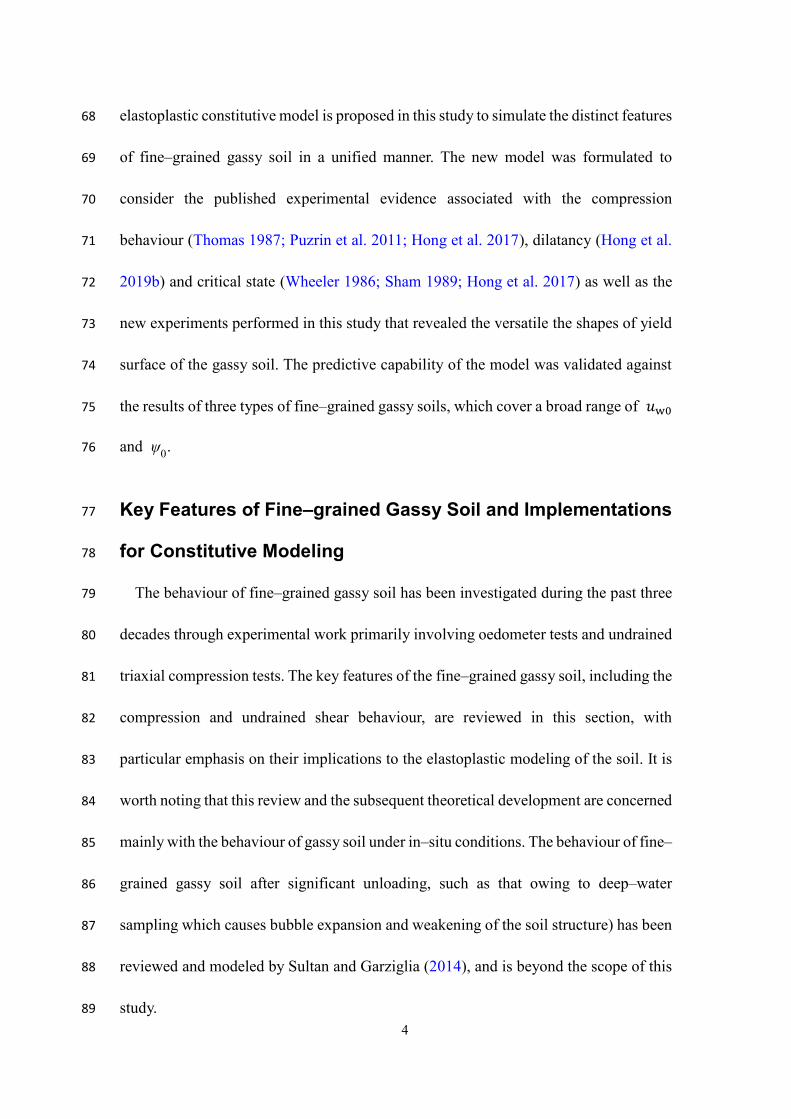
By considering the key features of fine–grained gassy soil, as reviewed in the 179
preceding section, a new elastoplastic model was developed within the framework of 180
critical state soil mechanics. The model consists of two parts, as shown in Fig. 3: (I) the 181
stress–strain behaviour of the saturated matrix, which is governed by the effective stress 182
principle, and (II) the volume change of gas bubbles owing to gas compression, which 183
is governed by the Boyle’s law. The modeling of unsaturated soils requires the proper 184
selection of stress variables (Alonso et al. 1990; Sun et al. 2000; Zhou and Sheng 2015; 185
Zhou and Ng 2016; Gallipoli et al. 2018). It has been justified theoretically (Xu and Xie 186
2011) and experimentally (Sills et al. 1991; Hong et al. 2017) that the effective stress 187
principle still applies for fine–grained gassy soil with 𝑆r exceeding 90%. The usage of 188
effective stress, therefore, has been reported to enable consistent interpretation 189
regarding the analysis of various behaviour of fine–grained gassy soil (𝑆r > 90%), as 190
revealed by consolidation analysis (Puzrin et al. 2011) and constitutive modeling 191
(Grozic et al. 2005; Sultan and Garziglia 2014) of the soil. 192
The total volumetric strain of fine–grained gassy soil is a sum of both the volumetric 193
strain of the saturated matrix and gas bubbles (Thomas 1987; Puzrin et al. 2011; Hong 194
et al. 2017). However, the global shear strain of a fine–grained gassy soil is assumed to 195
be identical to that of the saturated matrix because the gas bubbles, with zero shear 196

10
stiffness, have to deform compatibly with the saturated matrix (Wheeler 1986). 197
The following sub–sections aim to formulate the stress–strain behaviour of the 198
saturated matrix, except the last sub–section titled “Volumetric behaviour of gas 199
bubbles,” which describes the volumetric strain caused by gas compression. 200
Strain decomposition 201
Within the elasto–plastic framework, the strain rate tensor (d𝜀𝑖𝑗 ) of the saturated 202
matrix is decomposed into a plastic part (d𝜀𝑖𝑗p ) and an elastic part (d𝜀𝑖𝑗
e ): 203
d𝜀𝑖𝑗 = d𝜀𝑖𝑗e + d𝜀𝑖𝑗
p (4)
It is assumed that the saturated soil matrix behaves elastically when its stress state 204
remains within the yield surface, whereas plastic strain is developed once the yield 205
surface is reached. In the triaxial strain space, the work conjugate strain rates for 𝑝′ 206
and 𝑞 are the volumetric strain increment (d𝜀v = d𝜀1 + 2d𝜀3 , where d𝜀1 and d𝜀3 207
are the major and minor principal strain increments, respectively) and the deviatoric 208
strain increment (d𝜀q = 2(d𝜀1 − d𝜀3) 3⁄ ) of the saturated matrix, respectively. Further, 209
d𝜀v and d𝜀q are decomposed into: 210
d𝜀v = d𝜀ve + d𝜀v
p (5)
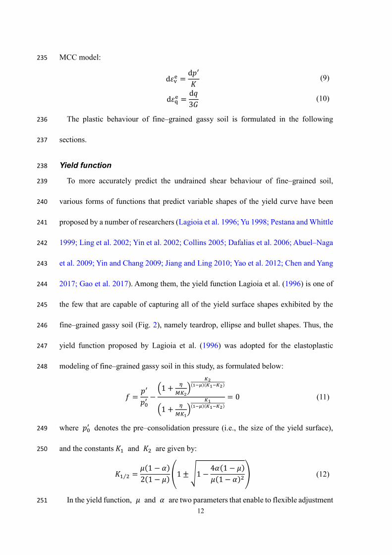
d𝜀q = d𝜀qe + d𝜀q
p (6)
where d𝜀ve and d𝜀v
p denote elastic and plastic volumetric strain increments, 211
respectively, and d𝜀qe and d𝜀q
p are elastic and plastic deviatoric strain increments, 212
respectively. The potential occurrence of bubble flooding, which would impose 213
additional volumetric strain to the saturated matrix by entry of water into the bubble 214
cavity (Wheeler 1988b), has not been considered in this proposed model. It was found 215

11
experimentally that bubble flooding may rarely occur during undrained shearing (Sham 216
1989). This was concluded from several undrained triaxial compression tests on gassy 217
Kaolin clayey specimens, which covered a broad range of initial degree of saturation 218
(𝑆r0=92.3% to 99.3%) and initial pore water pressure (𝑢w0=100 to 500 kPa). During 219
the undrained shearing of these gassy specimens, the deduced pore gas pressure (based 220
on the measured gas volume change and Boyle’s law) mainly stayed above the 221
measured pore water pressure, suggesting rare occurrence of bubble flooding. 222
For simplicity, the model is first presented for the triaxial space. More generalized 223
expressions of the model for the multi–axis condition are given in the Appendix. 224
Elastic behaviour 225
The elastic behaviour of the saturated matrix is assumed to be isotropic, as routinely 226
exercised in constitutive models for soft clay (Wheeler et al. 2003; Huang et al. 2011; 227
Wang et al. 2012, 2016). The isotropic elastic behaviour is described by the bulk and 228
shear moduli, i.e., 𝐾 and 𝐺, respectively, which are stress–dependent (as a function 229
of 𝑝′), as follows: 230
𝐾 =𝑝′
𝜅 (1 + 𝑒w0)⁄ (7)
𝐺 =3(1 − 2𝜈)2(1 + 𝜈) 𝐾 =
3(1 − 2𝜈)2(1 + 𝜈)
𝑝′
𝜅 (1 + 𝑒w0)⁄ (8)
where 𝑒w0 is the initial water void ratio of the gassy soil; 𝜅 is the slope of the elastic 231
swelling lines in the 𝑒w − ln𝑝′ plane; 𝜈 denotes Poisson’s ratio. According to the 232
theory of elasticity, the elastic increments of volumetric and deviatoric strain can be 233
readily calculated using Eqs. (9) and (10), which are the same as those adopted in the 234
12
MCC model: 235
d𝜀ve =
d𝑝′
𝐾 (9)
d𝜀qe =
d𝑞3𝐺
(10)
The plastic behaviour of fine–grained gassy soil is formulated in the following 236
sections. 237
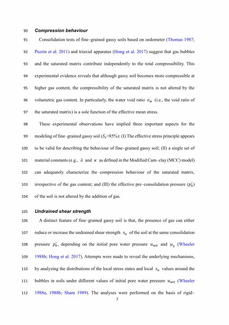
Yield function 238
To more accurately predict the undrained shear behaviour of fine–grained soil, 239
various forms of functions that predict variable shapes of the yield curve have been 240
proposed by a number of researchers (Lagioia et al. 1996; Yu 1998; Pestana and Whittle 241
1999; Ling et al. 2002; Yin et al. 2002; Collins 2005; Dafalias et al. 2006; Abuel–Naga 242
et al. 2009; Yin and Chang 2009; Jiang and Ling 2010; Yao et al. 2012; Chen and Yang 243
2017; Gao et al. 2017). Among them, the yield function Lagioia et al. (1996) is one of 244
the few that are capable of capturing all of the yield surface shapes exhibited by the 245
fine–grained gassy soil (Fig. 2), namely teardrop, ellipse and bullet shapes. Thus, the 246
yield function proposed by Lagioia et al. (1996) was adopted for the elastoplastic 247
modeling of fine–grained gassy soil in this study, as formulated below: 248
𝑓 =𝑝′
𝑝0′ −
(1 + 𝜂𝑀𝐾2
)𝐾2
(1−𝜇)(𝐾1−𝐾2)
(1 + 𝜂𝑀𝐾1
)𝐾1
(1−𝜇)(𝐾1−𝐾2)
= 0 (11)
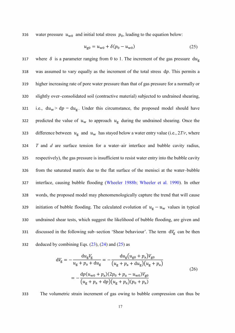
where 𝑝0′ denotes the pre–consolidation pressure (i.e., the size of the yield surface), 249
and the constants 𝐾1 and 𝐾2 are given by: 250
𝐾1 2⁄ =𝜇(1 − 𝛼)2(1 − 𝜇) (1 ± √1 −
4𝛼(1 − 𝜇)𝜇(1 − 𝛼)2) (12)
In the yield function, 𝜇 and 𝛼 are two parameters that enable to flexible adjustment 251
13
of the shapes of the yield surface. Fig. 4 shows the variations in the yield surface shape 252
with different values of 𝛼 between 0.03 and 2 but at a constant 𝜇=0.915. As illustrated, 253
the increase in the 𝛼 value from 0.03 to 2 led to a transition of the yield surface shape 254
on the wet side of the CSL in the following manner: bullet, ellipse, and teardrop shapes. 255
Specifically, this resulted in a yield surface similar to that of the MCC model, when D 256
= 0.4 and 𝜇 = 0.915. 257
One novel contribution in the gassy soil modeling of this study is to investigate and 258
formulate the dependency of the yield surface shape on the key factors governing the 259
yielding of fine–grained gassy soil (e.g., 𝑢w0 and ψ0 ). The functional form of 260
𝛼 (𝑢w0−𝑢w0_ref𝑝0
′ ,\0)is proposed considering the experimental observations, as presented 261
in the section titled “Experimental Investigation of Yield Curve and Flow Rule”. 262
Flow rule 263
As presented, the yield function 𝑓 (Eq. (11)) and the dilatancy function 𝐷 (Eq. (1)) 264
were independently formulated in accordance with the experimental evidences. A non–265
associated flow rule was thus naturally adopted in the proposed gassy soil model (see 266
also Gao et al. 2017): 267
d𝜀qp = ⟨𝐿⟩ 𝜕𝑓
𝜕𝑞 and d𝜀v
p = ⟨𝐿⟩ 𝜕𝑓𝜕𝑞
𝐷 (13)
where 𝐿 denotes the loading index. The McCauley brackets <> operate in the way 268
of ⟨𝑥⟩ = 𝑥 if 𝑥 > 0; otherwise, ⟨𝑥⟩ = 0. Direct experimental evidence for the non–269
associated flow rule is given in the following section. It should be noted that Eq. (13) 270
is an alternative method of defining the non–associated flow rule without explicitly 271
giving the plastic potential function. 272

14
Hardening and plastic modulus 273
Similar to the MCC model, the strain hardening hypothesis is invoked herein, with 274
the plastic volumetric strain increment of the saturated matrix (d𝜀vp) taken as the sole 275
internal variable for characterizing the evolution of the internal soil structure during the 276
plastic yielding. The following isotropic hardening law (as in MCC) is adopted to relate 277
the expansion or shrinkage of the yield surface size (d𝑝0′ ) to the internal variable (d𝜀v
p): 278
d𝑝0′ =
(1 + 𝑒w0)𝜆 − 𝜅
𝑝0′ d𝜀v
p (14)
The plastic volumetric strain increment d𝜀vp can be calculated by applying the 279
condition of consistency, which ensures that the stress state remains on the yield surface 280
during the plastic yielding, as follows: 281
d𝑓 =𝜕𝑓𝜕𝑝′ d𝑝′ +
𝜕𝑓𝜕𝑞
d𝑞 +𝜕𝑓𝜕𝑝0
′𝜕𝑝0
′
𝜕𝜀vp d𝜀v
p = 0 (15)
In Eq. (15), the derivatives 𝜕𝑓𝜕𝑝′,
𝜕𝑓𝜕𝑞
and 𝜕𝑓𝜕𝑝0
′ can be solved on the basis of the yield 282
function (Eq. (11)), and are given below: 283
𝜕𝑓𝜕𝑝′ =
1𝑝0
′ +(1 + 𝜂
𝑀𝐾2)
𝐾2(1−𝜇)(𝐾1−𝐾2)
(1 − 𝜇)(𝐾1 − 𝐾2) (1 + 𝜂𝑀𝐾1
)𝐾1
(1−𝜇)(𝐾1−𝐾2)
(1
1 + 𝜂𝑀𝐾2
−1
1 + 𝜂𝑀𝐾1
)𝑞
𝑀𝑝′2
(16a)
𝜕𝑓𝜕𝑞
= −(1 + 𝜂
𝑀𝐾2)
𝐾2(1−𝜇)(𝐾1−𝐾2)
(1 − 𝜇)(𝐾1 − 𝐾2) (1 + 𝜂𝑀𝐾1
)𝐾1
(1−𝜇)(𝐾1−𝐾2)
(1
1 + 𝜂𝑀𝐾2
−1
1 + 𝜂𝑀𝐾1
)1
𝑀𝑝′
(16b)
𝜕𝑓𝜕𝑝0
′ = −𝑝′
𝑝0′2 (16c)
According to the theory of plasticity (Dafalias 1986), Eq. (15) can be further 284
15
expressed as a function of the plastic modulus 𝐾p and the loading index 𝐿, as follows: 285
d𝑓 =𝜕𝑓𝜕𝑝′ d𝑝′ +
𝜕𝑓𝜕𝑞
d𝑞 − ⟨𝐿⟩𝐾p = 0 (18)
Combining Eqs. (15) and (18) leads to the following expression of 𝐾p: 286
𝐾p = −1𝐿
𝜕𝑓𝜕𝑝0
′𝜕𝑝0
′
𝜕𝜀vp d𝜀v
p (19)
Substituting Eqs. (13) and (14) into Eq. (19) yields: 287
𝐾p = −(1 + 𝑒w0)𝑝0
′
𝜆 − 𝜅𝜕𝑓𝜕𝑝0
′𝜕𝑓𝜕𝑞
𝐷
= −(1 + 𝑒w0)𝑝0
′
𝜆 − 𝜅𝜕𝑓𝜕𝑝0
′𝜕𝑓𝜕𝑞
[1 + 𝜉𝑢w0 − 𝑢w0_ref
𝑝0′ exp (−
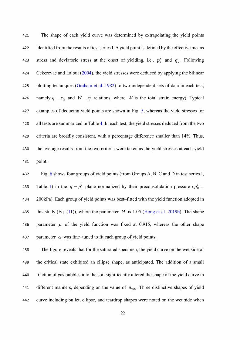
𝜒\0
)]𝑀2 − 𝜂2
2𝜂
(20)
With a known 𝐾p, the loading index 𝐿 can be readily calculated by the following 288
equation derived through standard elasto–plasticity procedures: 289
𝐿 =𝐾 𝜕𝑓
𝜕𝑝′ d𝜀v + 3𝐺 𝜕𝑓𝜕𝑞
d𝜀q
𝐾p + 𝐾 𝜕𝑓𝜕𝑝′
𝜕𝑓𝜕𝑞
𝐷 + 3𝐺 𝜕𝑓𝜕𝑞
𝜕𝑓𝜕𝑞
(21)
Elasto–plastic relation of the saturated soil matrix 290
Having defined the elastic incremental relationship (Eqs. (9) and (10)), and derived 291
the plastic modulus 𝐾p (Eq. (19)) as well as the loading index 𝐿 (Eq. (20)), the 292
elastoplastic relationship can be readily determined. In the triaxial stress space, the 293
incremental stress strain relationship is: 294
{d𝑝′
d𝑞 } = 𝐶2×2 {d𝜀vd𝜀q
} (21)
where 𝐶2×2 denotes the elastoplastic matrix, which can be explicitly expressed as: 295
𝐶2×2 = [𝐾 00 3𝐺] −
ℎ(𝐿)
𝐾p + 𝐾 𝜕𝑓𝜕𝑝′
𝜕𝑓𝜕𝑞
𝐷 + 3𝐺 𝜕𝑓𝜕𝑞
𝜕𝑓𝜕𝑞 [
𝐾2 𝜕𝑓
𝜕𝑝′𝜕𝑓𝜕𝑞
𝐷 3𝐺𝐾𝜕𝑓𝜕𝑞
𝜕𝑓𝜕𝑞
𝐷
3𝐺𝐾𝜕𝑓𝜕𝑝′
𝜕𝑓𝜕𝑞
9𝐺2 𝜕𝑓𝜕𝑞
𝜕𝑓𝜕𝑞 ]
(22)
16
Each term involved in the elastoplastic relation has been derived in the preceding 296
sub–sections. The Heaviside step function ℎ(𝐿) in Eq. (22) works as that ℎ(𝐿) = 1 297
if 𝐿 > 0, and ℎ(𝐿) = 0 if otherwise. 298
The derived constitutive relation (Eqs. (21) and (22)) has enabled the calculation of 299
deviatoric and volumetric strain increments for the saturated matrix with any given 300
stress increments (i.e., d𝑝′ and d𝑞). The former is identical to the global deviatoric 301
strain increment of the fine–grained gassy soil. The latter, in conjunction with the 302
volumetric strain of gas bubbles, as formulated in the following sub–section), form the 303
global volumetric strain of the fine–grained gassy soil. 304
Volumetric behaviour of gas bubbles 305
Considering that the typical types of bio–gas (i.e., methane and nitrogen (Lin et al. 306
2004; Wang et al. 2019)) have extremely low solubility, their volumetric behaviour is 307
predominately induced by gas compression. This can be described using Boyle’s law, 308
as follows: 309
(𝑢g + 𝑝a)𝑉g = (𝑢g + 𝑝a + d𝑢g)(𝑉g + d𝑉g) = 𝑛g𝑅𝑇 = 𝐶 (23)
where 𝑢g, 𝑝a, 𝑉g, 𝑛g, 𝑅, and 𝑇 denote the pore gas pressure, atmospheric pressure, 310
gas volume, number of the mole of the gas, ideal gas constant and absolute temperature, 311
respectively; and d𝑢g and d𝑉g are increment of gas pressure and gas volume, 312
respectively; The constant 𝐶 can be calculated by the initial pore gas pressure 𝑢g0 313
and the initial gas volume 𝑉g0 as 314
(𝑢g0 + 𝑝a)𝑉g0 = 𝐶 (24)
According to Sham (1989), the initial gas pressure 𝑢g0 falls between the initial pore 315
17
water pressure 𝑢w0 and initial total stress 𝑝0, leading to the equation below: 316
𝑢g0 = 𝑢w0 + 𝛿(𝑝0 − 𝑢w0) (25)
where 𝛿 is a parameter ranging from 0 to 1. The increment of the gas pressure d𝑢g 317
was assumed to vary equally as the increment of the total stress d𝑝. This permits a 318
higher increasing rate of pore water pressure than that of gas pressure for a normally or 319
slightly over–consolidated soil (contractive material) subjected to undrained shearing, 320
i.e., d𝑢w > d𝑝 = d𝑢g . Under this circumstance, the proposed model should have 321
predicted the value of 𝑢w to approach 𝑢g during the undrained shearing. Once the 322
difference between 𝑢g and 𝑢w has stayed below a water entry value (i.e., 2T/r, where 323
T and d are surface tension for a water–air interface and bubble cavity radius, 324
respectively), the gas pressure is insufficient to resist water entry into the bubble cavity 325
from the saturated matrix due to the flat surface of the menisci at the water–bubble 326
interface, causing bubble flooding (Wheeler 1988b; Wheeler et al. 1990). In other 327
words, the proposed model may phenomenologically capture the trend that will cause 328
initiation of bubble flooding. The calculated evolution of 𝑢g − 𝑢w values in typical 329
undrained shear tests, which suggest the likelihood of bubble flooding, are given and 330
discussed in the following sub–section ‘Shear behaviour’. The term d𝑉g can be then 331
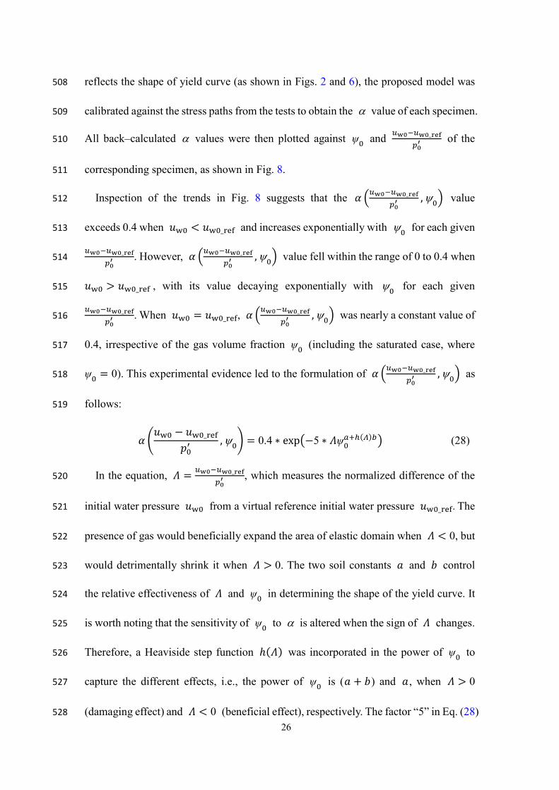
deduced by combining Eqs. (23), (24) and (25) as 332
d𝑉g = −d𝑢g𝑉g
𝑢g + 𝑝a + d𝑢g= −
d𝑢g(𝑢g0 + 𝑝a)𝑉g0
(𝑢g + 𝑝a + d𝑢g)(𝑢g + 𝑝a)
= −d𝑝(𝑢w0 + 𝑝a)(2𝑝0 + 𝑝a − 𝑢w0)𝑉g0
(𝑢g + 𝑝a + d𝑝)(𝑢g + 𝑝a)(𝑝0 + 𝑝a)
(26)
The volumetric strain increment of gas owing to bubble compression can thus be 333

18
obtained, as follows: 334
d𝜀vg =
d𝑉g
𝑉= −
d𝑝(𝑢w0 + 𝑝a)(2𝑝0 + 𝑝a − 𝑢w0)ψ0
(𝑢g + 𝑝a + d𝑝)(𝑢g + 𝑝a)(𝑝0 + 𝑝a) (27)
The above formulations were derived following the routine practice (Thomas 1987; 335
Wheeler 1988a; Wheeler et al. 1990) for estimating gas pressure and volumetric 336
behaviour of gas bubbles using Boyle’s law. In this simplified approach, the effect of 337
changing surface tension (by the small menisci forming at the interface between the gas 338
bubbles and pore water) on gas pressure variation has not been explicitly considered. 339
This could have led to some errors in predicting the volumetric behaviour of gas 340
bubbles, as detailed in the section “Compression behaviour”. On the other hand, the 341
capability of the proposed model for predicting the shear behaviour of the saturated 342
matrix, which is a primary focus of this study, is merely affected by the simplification 343
using Boyle’s law. Because the only gas–related variable governing the shear behaviour 344
is the initial gas volume fraction, which is measurable experimentally. 345
It is worth noting that the model proposed herein was derived by assuming that the 346
discrete bubbles form stably within the soil, which consistently impose a certain degree 347
of detrimental or beneficial effect in the soil. This assumption has been justified 348
experimentally by Hong et al. (2017). In their triaxial test, a constant isotropic cell 349
pressure of 320 kPa and back pressure of 120 kPa were imposed to a gassy specimen 350
for 24 h, which is twice of the duration required for a typical undrained triaxial 351
compression test for fine–grained gassy soil. The total volume of the gassy specimen 352
under the constant load was almost identical, which suggests that the nitrogen bubbles 353
were stably formed and their modification effect on the soil did not vanish with time. 354
19
Experimental Investigation of Yield Curve and Flow Rule 355
A series of undrained triaxial tests was conducted on reconstituted gassy Malaysia 356
kaolin. The primary objectives of the experimental investigation were (Ⅰ) to verify the 357
modeling concepts incorporated in the new model, particularly the hypothesized shapes 358
of yield curve and non–associated flow rule, and (Ⅱ) to formulate the dependency of 359
the yield surface shape on the key factors governing the yielding of fine–grained gassy 360
soil, i.e., a functional form 𝛼 (𝑢w0−𝑢w0_ref𝑝0
′ ,\0) related to the yield curve shape. 361
Several preliminary test results are reported in Hong et al. (2019b). 362
Experimental program and setup 363
The program consists of two series of strain–controlled undrained triaxial 364
compression tests. The test series I and II aimed to address the afore mentioned 365
objectives (Ⅰ) and (Ⅱ), respectively. The program of test series II and part of the 366
experimental data had been reported in Hong et al. (2019b). 367
In test series I, a total of 24 tests were performed on OC specimens under an isotropic 368
stress condition. As summarized in Table1, the program was divided into four groups 369
including Groups A, B and C for gassy specimens containing the same amount of gas, 370
4.6 x10⁻⁴ mole, at different values of 𝑢w0 at 0, 150, and 600 kPa, and Group D for 371
saturated specimens. Each group consisted six specimens, having the same size of yield 372
surface, 𝑝0′ = 200kPa but with different current effective mean stresses, at 𝑝i
′=120, 373
140, 160, 170 180, and 190 kPa. The undrained shear tests of the six OC specimens in 374
each group led to the identification of six yield points that defined the shape of the yield 375
curve and the directions of the plastic strain increments at the six points. 376
20
Test series II included 18 tests on gassy specimens and 1 reference test on a saturated 377
specimen, as summarized in Table 2. The experimental program considered a wide 378
range of initial pore water pressures, at 𝑢w0 = 0 − 600kPa , and initial gas volume 379
fractions, at ψ0 = 0.6 − 6.3%, aiming to offer representative experimental results for 380
formulating the shape–related functional form 𝛼 (𝑢w0−𝑢w0_ref𝑝0
′ ,\0). 381
The experimental investigation was performed using a GDS triaxial apparatus 382
equipped with a HKUST double–cell (Ng et al. 2002) for measuring changes in the 383
degree of saturation (Sr) and gas volume fraction (ψ) during the test of each gassy 384
specimen. All of the tests were performed in a lab with controlled room temperature at 385
T=25or 2o. The double cell system was calibrated to account for the apparent volume 386
change caused by the deformation of the inner cell and drainage lines owing to variation 387
in cell pressure, temperature and creep, and by the movement of the loading ramp 388
relative to the inner cell (Ng et al. 2002). The estimated accuracy of the double–cell 389
system was equivalent to a volumetric strain of 0.05 % for each gassy specimen. 390
Testing material and preparation of gassy specimen 391
Given the difficulty in obtaining intact gassy samples from the field owing to gas 392
expansion upon unloading, reconstituted gassy specimens were replicated in this 393
experimental investigation, as routinely exercised in relevant studies (Wheeler 1988b; 394
Sham 1989; Lunne et al. 2001; Sultan et al. 2012).The gassy specimens were prepared 395
by introducing nitrogen, a typical bio–gas, into saturated Malaysia kaolin using the 396
zeolite molecular sieve technique (Nageswaran 1983). Table 3 shows the index 397
properties of the kaolin. This technique been used to yield repeatable gassy specimens 398
21
with controllable gas contents (Wheeler 1988b; Sham 1989; Hong et al. 2017). Details 399
of this technique are given in Nageswaran (1983). 400
The replicated gassy soils were carefully trimmed to form standard triaxial specimens 401
with a diameter and height of 50 mm by 100 mm, respectively. They were then 402
transferred to the triaxial cell for isotropic consolidation under the same 𝑝0′ (i.e., 200 403
kPa) but different 𝑢w0 values (i.e., 0, 50, 150, 300 and600 kPa). 404
Experimental procedure 405
Each test in series I, as listed in Table 1, were performed according to the following 406
procedures: 407
1. impose a drained isotropic unloading path to each normally consolidated gassy 408
specimen, to bring its stress state to different points within the yield surface such as 409
120, 140, 160, 170, 180, and 190 kPa; 410
2. applying undrained triaxial compression to each specimen at a constant axial strain 411
rate of 1.5%/h until reaching the critical state; 412
3. forcibly saturate each specimen by increasing the cell pressure (under the undrained 413
condition) until no further development of volume change is noted. This procedure 414
is used to obtain the final gas volume after reaching the critical state, and thus to 415
back–calculate the values of 𝑆r and ψ during the entire process of each test 416
(Wheeler 1988b; Sham 1989; Hong et al. 2017). 417
The tests in series II (Table 2) were performed following procedures (2) and (3), as 418
listed above. 419
Distinct shapes of yield curve 420
22
The shape of each yield curve was determined by extrapolating the yield points 421
identified from the results of test series I. A yield point is defined by the effective means 422
stress and deviatoric stress at the onset of yielding, i.e., 𝑝y′ and 𝑞y . Following 423
Cekerevac and Laloui (2004), the yield stresses were deduced by applying the bilinear 424
plotting techniques (Graham et al. 1982) to two independent sets of data in each test, 425
namely 𝑞 − 𝜀q and 𝑊 − 𝜂 relations, where 𝑊 is the total strain energy). Typical 426
examples of deducing yield points are shown in Fig. 5, whereas the yield stresses for 427
all tests are summarized in Table 4. In each test, the yield stresses deduced from the two 428
criteria are broadly consistent, with a percentage difference smaller than 14%. Thus, 429
the average results from the two criteria were taken as the yield stresses at each yield 430
point. 431
Fig. 6 shows four groups of yield points (from Groups A, B, C and D in test series I, 432
Table 1) in the 𝑞 − 𝑝′ plane normalized by their preconsolidation pressure (𝑝0′ =433
200kPa). Each group of yield points was best–fitted with the yield function adopted in 434
this study (Eq. (11)), where the parameter 𝑀 is 1.05 (Hong et al. 2019b). The shape 435
parameter P of the yield function was fixed at 0.915, whereas the other shape 436
parameter D was fine–tuned to fit each group of yield points. 437
The figure reveals that for the saturated specimen, the yield curve on the wet side of 438
the critical state exhibited an ellipse shape, as anticipated. The addition of a small 439
fraction of gas bubbles into the soil significantly altered the shape of the yield curve in 440
different manners, depending on the value of 𝑢w0. Three distinctive shapes of yield 441
curve including bullet, ellipse, and teardrop shapes were noted on the wet side when 442
23
relatively high, intermediate, and very low values of 𝑢w0 at 600 kPa, 150 kPa, and 0 443
kPa were imposed, respectively. 444
Although the yield function (i.e., Eq. (11)) is defined based on stresses within the 445
matrix, it is still likely to be valid for describing the overall yield behaviour of soils 446
containing a small fraction of gas, where the effective stress principle approximately 447
works for the entire gassy soil. Xu and Xie (2011) derived the effective stress for fine–448
grained soil containing discrete bubbles based on three–phase equilibrium analysis of a 449
representative element volume (REV), as a function of total stress, pore water pressure, 450
pore gas pressure and surface tension. Using their equation, it can be readily calculated 451
that for all the gassy specimens summarized in Table 1 (for studying yield loci), the 452
initial effective mean stress 𝑝′ in saturated matrix of each specimen only deviates from 453
the corresponding ‘overall’ 𝑝′ of the entire gassy specimen by 1% (i.e., 1.2 kPa for 454
specimen G0_120). Meanwhile, the ‘overall’ deviatoric stress imposed to each gassy 455
specimen is anticipated to be the same as that taken locally by the saturated matrix, 456
because the gas bubbles cannot sustain shear stress. It is therefore a reasonable 457
approximation to use the yield function based on stresses defined for the saturated 458
matrix (Eq. (11)) to describe the overall yield behaviour of soils containing a small 459
fraction of gas. 460
The observed shapes of the yield loci have revealed the underlying mechanisms of 461
the gas bubble effect in the context of elasto–plastic modeling. The presence of gas 462
bubbles at a relatively high 𝑢w0 value (600 kPa) led to shrinkage of the area of elastic 463
domain, as compared with that of the saturated specimen. This is likely associated with 464
24
the localized shear failure induced initially in the saturated matrix surrounding the 465
bubbles, which plays a dominant role at high 𝑢w0 (Wheeler 1988b; Sham 1989). 466
Conversely, the presence of gas bubbles at a low 𝑢w0 (0 kPa) resulted in an expanded 467
area of elastic domain relative to that of the saturated specimen. This is likely attributed 468
to the dominant effect of localized matrix heterogeneity at low 𝑢w0, which causes the 469
saturated matrix around the gas bubbles to be lightly OC, thus expanding the yield 470
surface (Sham 1989). The area of the elastic domain at a moderate 𝑢w0 of 150 kPa 471
was quite similar to that of the saturated specimen, which suggests that the effects of 472
the aforementioned competing mechanisms are likely cancelled out under this 473
circumstance. This experimental evidence verifies the concept of adopting a versatile 474
expression of the yield function (Eq. (11)) in the proposed model, which can reproduce 475
the three distinct shapes of the yield curve by varying the shape parameter D. To enable 476
unified modeling of the variable yield curves of the gassy soil with a single set of 477
parameters, the term D should be formulated as a functional form that adequately 478
captures the combined effects of 𝑢w0 and ψ0 . The functional form is proposed 479
subsequently, based on the results of test series II. 480
Direction of plastic strain increment and flow rule 481
Fig. 6 also shows the incremental plastic strain vector (i.e., resultant vector of d𝜀vp 482
and d𝜀qp) at each yield point. The increments of plastic volumetric and deviatoric strain, 483
which determines the direction of the incremental plastic strain vector, were calculated 484
using Eqs. (5), (6), (9) and (10). In the calculation, the stress increment was taken as 485
20kPa, which is 1/10 of the pre–consolidation pressure 𝑝0′ (Cekerevac and Laloui 486
25
2004). 487
As illustrated, the direction of the plastic strain vectors of the saturated specimen 488
(Group D) and the gassy specimen at an intermediate 𝑢w0 = 150kPa (Group B) 489
aligned roughly perpendicular to their yield curves. The “deviation” of the plastic strain 490
increment vectors varied between –5˚ and 2˚, as summarized in Table 5. However, these 491
are significant deviations between the direction of the plastic strain vectors and the 492
normality of the yield curves, for the gassy specimens in Groups A and C with a low 493
and a relatively high 𝑢w0 of 0 and 600 kPa, respectively. The deviation angles were 494
in the range of –68˚ to 37˚ (Table 5). This verifies the concept of adopting a non–495
associated flow rule (Eq. (13)) in the proposed model. 496
The dependency of plastic flow direction (i.e., dilatancy) of fine–grained gassy soil 497
on 𝑢w0 and ψ0 was incorporated into the dilatancy function (as published in Hong et 498
al. 2019b). This was achieved by introducing a dilatancy multiplier 499
𝐹 (𝑢𝑤0−𝑢𝑤0_𝑟𝑒𝑓
𝑝0′
,\0) to scale the dilatancy function of the MCC model, as shown in Eq. 500
(1). Fig. 7 compares the measured and the predicted dilatancy multiplier 501
𝐹 (𝑢𝑤0−𝑢𝑤0_𝑟𝑒𝑓
𝑝0′ ,\0) deduced from results of test series I and II, which validate the 502
dilatancy function (Eq. (1)) used in the proposed model. 503
Formulating functional forms for 𝜶(𝒖𝒘𝟎−𝒖𝒘𝟎_𝒓𝒆𝒇
𝒑𝟎′ ,\𝟎) 504
Based on the results of test series I and II covering a broad range of 𝑢w0 and ψ0, 505
the dependency of the yield shape related functional forms 𝛼 (𝑢w0−𝑢w0_ref𝑝0
′ ,\0) on the 506
two variables can be formulated. Because the locus of the undrained effective stress 507
26
reflects the shape of yield curve (as shown in Figs. 2 and 6), the proposed model was 508
calibrated against the stress paths from the tests to obtain the D value of each specimen. 509
All back–calculated D values were then plotted against ψ0 and 𝑢w0−𝑢w0_ref𝑝0
′ of the 510
corresponding specimen, as shown in Fig. 8. 511
Inspection of the trends in Fig. 8 suggests that the 𝛼 (𝑢w0−𝑢w0_ref𝑝0
′ ,\0) value 512
exceeds 0.4 when 𝑢w0 < 𝑢w0_ref and increases exponentially with \0 for each given 513
𝑢w0−𝑢w0_ref𝑝0
′ . However, 𝛼 (𝑢w0−𝑢w0_ref𝑝0
′ ,\0) value fell within the range of 0 to 0.4 when 514
𝑢w0 > 𝑢w0_ref , with its value decaying exponentially with \0 for each given 515
𝑢w0−𝑢w0_ref𝑝0
′ . When 𝑢w0 = 𝑢w0_ref, 𝛼 (𝑢w0−𝑢w0_ref𝑝0
′ ,\0) was nearly a constant value of 516
0.4, irrespective of the gas volume fraction ψ0 (including the saturated case, where 517
ψ0 = 0). This experimental evidence led to the formulation of 𝛼 (𝑢w0−𝑢w0_ref𝑝0
′ ,\0) as 518
follows: 519
𝛼 (𝑢w0 − 𝑢w0_ref
𝑝0′ ,\0) = 0.4 ∗ exp(−5 ∗ 𝛬ψ0
𝑎+ℎ(𝛬)𝑏) (28)
In the equation, 𝛬 = 𝑢w0−𝑢w0_ref𝑝0
′ , which measures the normalized difference of the 520
initial water pressure 𝑢w0 from a virtual reference initial water pressure 𝑢w0_ref. The 521
presence of gas would beneficially expand the area of elastic domain when 𝛬 < 0, but 522
would detrimentally shrink it when 𝛬 > 0. The two soil constants 𝑎 and 𝑏 control 523
the relative effectiveness of 𝛬 and ψ0 in determining the shape of the yield curve. It 524
is worth noting that the sensitivity of ψ0 to D is altered when the sign of 𝛬 changes. 525
Therefore, a Heaviside step function ℎ(𝛬) was incorporated in the power of ψ0 to 526
capture the different effects, i.e., the power of ψ0 is (𝑎 + 𝑏 ) and 𝑎 , when 𝛬 > 0 527
(damaging effect) and 𝛬 < 0 (beneficial effect), respectively. The factor “5” in Eq. (28) 528

27
is a default value independent of the initial conditions (including ψ0 and 𝑢w0) and the 529
soil type, as evident from the three types of fine–grained gassy soils simulated in this 530
study (Table 6). 531
The proposed form of 𝛼 (𝑢w0−𝑢w0_ref𝑝0
′ ,\0) can capture the following key features of 532
fine–grained gassy soils: 533
1. When 𝑢w0 > 𝑢w0_ref, the shape–related term D is smaller than 0.4, causing a bullet 534
shape in the yield curve. This simulates the detrimental role of gas in shrinking the 535
area of elastic domain. 536
2. When 𝑢w0 < 𝑢w0_ref, the shape–related term D exceeds 0.4, causing a teardrop 537
shape in the yield curve. This models the beneficial role of gas in expanding the 538
area of elastic domain. 539
3. When 𝑢w0 = 𝑢w0_ref, the shape–related term D becomes 0.4. For this special case, 540
the shape of the yield curve is very close to an ellipse, and the gassy soil behaves 541
similarly to its saturated equivalent. 542
4. Upon reaching saturation (\0=0), D is equal to 0.4, irrespective of the 𝑢w0 values. 543
The shape of the yield curve becomes very similar to that of the MCC, and the 544
proposed model is recovered to a conventional critical state model for saturated 545
fine–grained soil. 546
Determination of Model Parameters 547
Standard experimental procedure for parameter determination 548
The new model includes ten parameters. In addition to the five conventional 549
parameters of O , 𝜅 , 𝑁 , 𝑣 , and 𝑀 from the MCC model, two new parameters 550
28
controlling the shape of the yield curve (𝑎 and 𝑏) and two new parameters governing 551
the stress–dilatancy (𝜉 and 𝜒 ) and one new parameter relating to the initial gas 552
pressure (G) are introduced in the new model. The parameter G is not compulsory, if 553
the prediction for the volumetric behaviour of the gassy soil were not intended. These 554
parameters can be conveniently determined from the results of conventional oedometer 555
and triaxial tests in the following ways: 556
1. The MCC model parameters O, 𝜅, 𝑁, 𝑣, and 𝑀 can be obtained following well–557
established procedures such as those recommended by Wood (1990), based on 558
conventional oedometer and triaxial tests conducted on saturated specimens; 559
2. 𝜉 and 𝜒 controlling the stress–dilatancy can be fine–tuned to fit the dilatancy 560
function (Eq. (1)) against the measured stress–dilatancy relations of fine–grained 561
gassy soil. Hong et al. (2019b) performed the calibration against the results of four 562
undrained triaxial tests, which were undertaken at two values of 𝑢w0 with one each 563
exceeding and remaining below 𝑢w0_ref, with two different values of \0 at each 564
𝑢w0. 565
3. 𝑎 and 𝑏 controlling the shape of the yield curve can be determined by calibrating 566
the undrained effective stress paths of the same triaxial tests mentioned in item (2) 567
on the basis of the seven pre–determined parameters (i.e., O, 𝜅, 𝑁, 𝑣, 𝑀, 𝜉, and 568
𝜒). 569
4. G can be tuned by fitting the compression curves of gassy specimen (under either 570
1D or isotropic conditions). 571
These procedures were used to determine the model parameters of three types of 572
29
fine–grained gassy soils published in the literature, as summarized in Table 6. The test 573
results of these fine–grained gassy soils were used for verifying the new model 574
proposed in this study, as presented in the following section. 575
Correlation of the four new model parameters to Atterberg limits 576
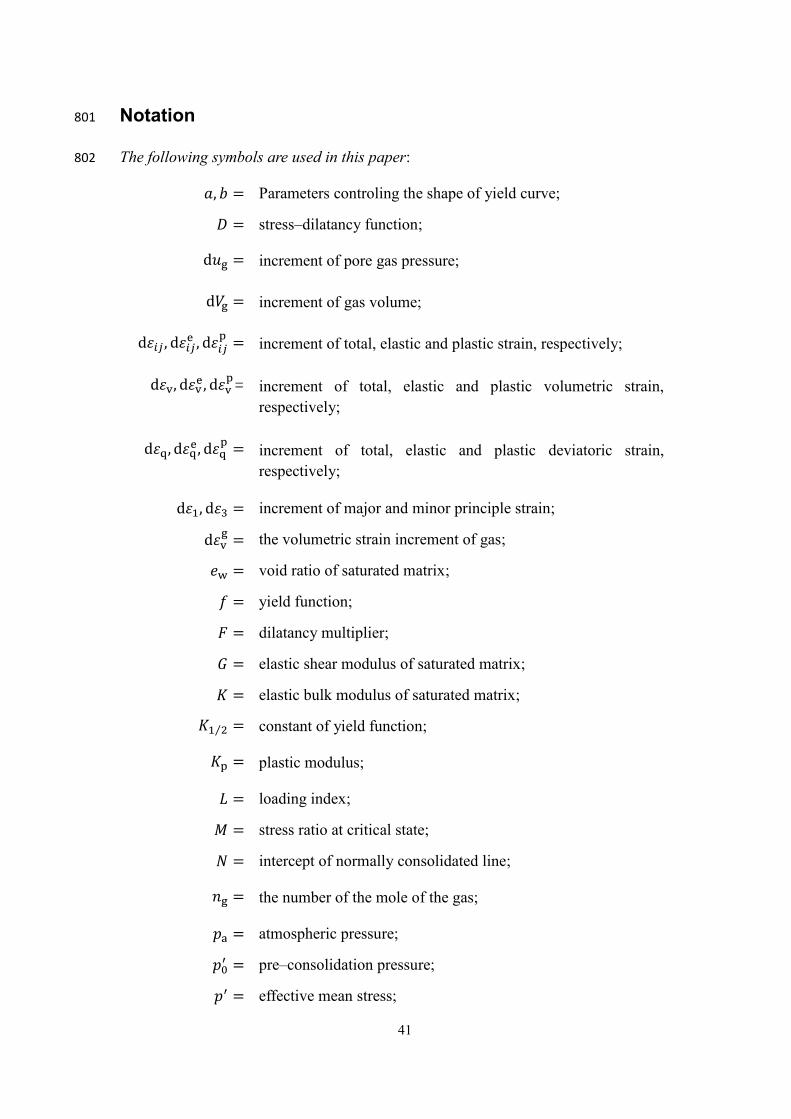
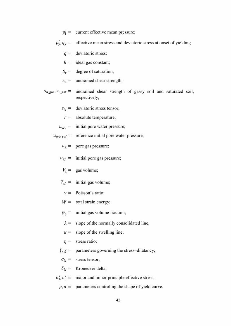
As shown in Table 6, the values of the new parameters (𝑎, 𝑏, 𝜉 and 𝜒) appeared to 577
vary significantly among the three gassy soils. An attempt was therefore made to 578
explore whether the new parameters followed a particular certain trend, by examining 579
their correlations to the intrinsic soil properties (e.g., Atterberg limits). It was 580
encouraging to find that each new model parameter exhibited an approximate linear 581
correlation to the plastic index (Ip) of the soils (see Fig. 9), with the coefficient of 582
determination (R2) for each parameter being no smaller than 0.87. These correlations 583
may offer an alternative way for estimating the four new model parameters, given the 584
lack of experimental results. 585
Model Validation 586
To adequately verify the new gassy soil model, all published experimental results, to 587
the authors’ best knowledge, on the behaviour of fine–grained gassy soil under in–situ 588
stress conditions without experiencing unloading were collected. These include tests on 589
three types of gassy fine–grained soils, i.e., gassy Combwich mud (Wheeler 1986; 590
Thomas 1987), gassy Kaolin clay (Sham 1989) and gassy Malaysia kaolin (Hong et al. 591
2019), which cover a wide range of initial pore water pressure of 0–600kPa and degree 592
of saturation 𝑆r at 88.2–100%. On the basis of their Atterberg limits, compared with 593
the values of the British Standards Institution (BSI, 1999), the Combwich mud, Kaolin 594
30
clay and Malaysia kaolin were characterized as silt with very high plasticity, clay with 595
high plasticity and silt with high plasticity, respectively. This suggests that the test 596
results adopted for validation are representative of those exhibited by most fine–grained 597
gassy soil. 598
The gassy soil specimens in the above experiments (including compression and 599
triaxial shear tests) for model validation were all prepared using the zeolite molecular 600
sieve technique, which closely mimic the process of bubble formation within fine–601
grained marine sediments (Sills et al. 1991). This is could have led to similar micro–602
structure of the three gassy soils, which could be simulated by the proposed model in a 603
consistent manner. 604
Compression behaviour 605
Figs. 10(a) and 10(b) show comparisons between the measured and predicted 606
compression behaviour of one–dimensionally consolidated Combwich mud (Thomas 607
1987) and isotopically consolidated Malaysia kaolin, respectively, with different \0. 608
The gassy Combwich mud specimens were charged with various amounts of methane 609
at \0=2.1% and 12.7% and were consolidated under 𝑢w0=0 kPa. The gassy Malaysia 610
kaolin specimens were charged with the same amount of nitrogen, which exhibited 611
different \0 between 0.7% and 9.2% owing to the varying values of 𝑢w0 imposed, 612
at 0–1000kPa. It can be seen from Figs. 10(a) and (b) that the proposed model can 613
broadly capture the compression behaviour of gassy and saturated specimen of the two 614
soils, with a maximum percentage difference of 17%. To improve the model prediction, 615
the effect of changing surface tension (by the small menisci forming at the water–gas 616
31
bubble interface) on gas pressure variation should be explicitly considered in future, 617
because the gas pressure affects the compression of the gas bubbles in this model. 618
While calculating the above compression curves with the proposed model, it was 619
found that the parameter G (controlling the initial gas pressure, see Eq. (25)) is a 620
material constant independent of the initial gas content and pore water pressure, i.e., G 621
= 0.6 and 0.7 for Combwich mud and Malaysia kaolin, respectively. This suggests the 622
validity of Sham (1989)’s equation as a first approximation for the initial gas pressure. 623
Shear behaviour 624
Fig. 11 compares the measured and predicted undrained shear behaviour (i.e., stress–625
strain relation, excess pore water pressure and effective stress path) of typical gassy 626
Malaysia kaolin specimens having a wide range of initial pore water pressure, at 627
𝑢w0=0–600 kPa) and gas volume fractions, at \0=0.6%–6.3%). As illustrated in the 628
figure, the proposed model is capable of reasonably reproducing the various shear 629
behaviour measured in the experiments. In particular, the proposed model managed to 630
capture the directions of the initial portions of the effective stress paths owing to a very 631
small d𝜂 of 𝜂=0, i.e., an initially inclining stress path (d𝑝′ < 0) for the gassy specimen 632
with 𝑢w0 = 600kPa, and a stress path with delayed inclining compared with that of 633
saturated specimen for the gassy specimen with 𝑢w0 = 0kPa. The former is associated 634
with an inelastic response during the very early stage of shearing (Yang et al. 2016), 635
whereas the latter implies a delayed onset of yielding compared with that of its saturated 636
equivalent). These features were reproduced by introducing the physically robust yield 637
function 𝑓 and the dilation function D in the proposed model, which reasonably 638
32
predicted the plastic volumetric strain (d𝜀vp = ⟨𝐿⟩ 𝜕𝑓
𝜕𝑞𝐷) and elastic volumetric strain 639
(d𝜀ep=−d𝜀v
p under the undrained condition), and thus d𝑝′ at very small 𝜂. 640
Figs. 12 and 13 show comparisons between the measured and predicted undrained 641
shear responses of gassy Combwich mud (Wheeler 1986) and gassy Kaolin clay (Sham 642
1989), respectively. Because only one set of data on the full curves of undrained shear 643
responses was reported for each soil (Figs. 11 and 12), it is not possible to rigorously 644
calibrate all parameters following the standard procedures suggested in the preceding 645
section. Trial–and–errors were employed to best–tune the model parameters, based on 646
the single set of data on the undrained shear responses, and the large numbers of 647
measured undrained shear strength for each soil. The model parameters of gassy 648
Combwich mud and gassy Kaolin clay are summarized in Table 6, while the calibrated 649
reference initial water pressure 𝑢w0_ref of the former and the latter are 20 kPa and 50 650
kPa, respectively. Given the lack of rigor in the calibration, the model predictions for 651
the two soils still show broadly agreements with the experimental results. 652
Undrained shear strength 653
Figs. 14, 15 and 16 show the comparisons between the measured and predicted 654
undrained shear strength (𝑠u) of gassy Malaysia kaolin silt, Combwich mud, and Kaolin 655
clay at various combinations of 𝑢w0 and ψ0, respectively. In each figure, the strength 656
of the gassy specimens (𝑠u_gas) was normalized by that of the saturated specimen (𝑠u_sat) 657
having the same 𝑝0′ . When the 𝑠u_gas 𝑠u_sat⁄ ratio was lower than the unity, the gas 658
bubbles posed a damaging effect to the soil, and vice versa. As shown in the figures, 659
the proposed model is able to capture both the damaging and beneficial effects of gas 660
33
on 𝑠u of the gassy soils for each soil, with a unified set of model parameters. 661
Quantitatively, the percentage difference between the measured and predicted values of 662
𝑠u for gassy Malaysia Kaolin silt, in which all model parameters were determined via 663
rigorous calibrations, was no larger than 10%. Higher percentage differences of 15% 664
and 16%were obtained when predicting 𝑠u for gassy Combwich mud and Kaolin clay, 665
respectively, owing to the lack of experimental results for rigorously calibrating their 666
model parameters, such as effective stress paths and stress–dilatancy relations at 667
different 𝑢w0 values. 668
Quantifying the ‘detrimental’ and ‘beneficial’ effect of gas: a 669
parametric study 670
Based on the validated model and model parameters of the three fine–gained gassy 671
soils, as presented above, a program of parametric study was performed to quantify the 672
modification effect of gas on the 𝑠u values of the gassy soils. For each soil, 10000 sets 673
of combinations that cover a broad range of initial pore water pressure (𝑢w0= 0–1000 674
kPa) and initial gas volume fraction (ψ0 = 0–10%) at a given initial effective stress 675
(𝑝0′ =200 kPa) were considered in the parametric study. 676
Fig. 17(a), 17(b) and 17(b) show the calculated results of gassy Malaysia kaolin 677
silt (Ip=27), gassy Combiwich mud (Ip=28) and gassy Kaolin clay (Ip=32), respectively. 678
In each figure, the undrained shear strength of gassy soil is normalized by that of its 679
saturated equivalent, i.e., 𝑠u_gas 𝑠u_sat⁄ , for identifying ‘detrimental’ or ‘beneficial’ 680
effect by presence of gas. It can be seen that the modification effect of gas on the 681
undrained shear strength of fine–grained soil greatly varies. Presence of gas can either 682

34
reduce undrained shear strength by 25%, or increase it by 40%, depending on the 683
coupling effect between ψ0 and 𝑢w0 (as featured by the dimensionless variable 𝛬). 684
For each soil with a given 𝛬, the change of soil strength by presence of gas (either 685
‘detrimental’ or ‘beneficial’) increases with initial gas volume fraction ψ0 , but at a 686
decreasing rate. The calculation charts, as shown in Fig. 17, may assist with the 687
preliminary design of offshore structures founded on a gas–bearing fine–grained 688
sediments with relevant plastic indexes (Ip). 689
Conclusions 690
This study presents a new elastoplastic critical state constitutive model for fine–691
grained gassy soil. The model was formulated for the triaxial and generalized three–692
dimensional (3D) stress conditions as described in the Appendix). 693
Unlike existing models which solely consider either detrimental or beneficial effect 694
of gas on fine–grained soil, the new model captures both the damaging and beneficial 695
effects of gas bubbles on the stress–strain behaviour of gassy soils in a unified manner. 696
This was achieved by incorporating a versatile expression of yield function and a 697
dilatancy function of gassy soils, which account for the coupling effects of ψ0 and 698
𝑢w0, into the elastoplastic framework in conjunction with the concept of critical state. 699
Compared with the MCC model, four additional model parameters are introduced in 700
the proposed model, for describing the effects of gas on the yield surface shape and 701
stress–dilatancy of fine–grained gassy soil. All parameters can be determined through 702
routine oedometer and triaxial tests. The four new model parameters almost linearly 703
correlated with the plastic index (Ip) of the soil, offering an alternative way to 704
35
approximate these parameters. 705
The proposed model reasonably predicted the behaviour of three different types of 706
fine–grained gassy soils covering a wide range ofψ0 and 𝑢w0 , with a single set of 707
parameters. The distinct features of the fine–grained gassy soil, which had been treated 708
separately or partly in the existing models, can now be captured by the new model 709
within a unified framework. The model’s benefits are summarized in the following 710
points. 711
1. The versatile expression of yield function can model, in a unified context, the 712
distinct shapes of yield curve such as bullet, ellipse, and teardrop shapes) for fine–713
grained gassy soils over a wide range of ψ0 and 𝑢w0. This has enabled the model 714
to consider the role of gas in either contracting or expanding the area of the elastic 715
domain at a given pre–consolidation pressure 𝑝0′ . 716
2. By suitable adjustment of the elastic domain area, the model can reproduce an 717
inelastic response during the very early stage of shearing (under a small d𝜂 at 𝜂 =718
0) of fine–grained gassy soil at a high 𝑢w0 or a delayed onset of yielding than that 719
of its saturated equivalent) for gassy soil with a low 𝑢w0. This explains the different 720
initial directions of their undrained effective stress paths, i.e., an initially inclined 721
stress path (d𝑝′ < 0 ) owing to an inelastic response and delayed inclination the 722
stress path when the elastic domain expands. 723
3. The adopted dilatancy function (as published in Hong et al. (2019b)) can model the 724
role of gas in either suppressing or enhancing the dilatancy of the gassy soil 725
compared with the ability of their saturated equivalents over a broad range of ψ0 726

36
and 𝑢w0 with one set of parameters. 727
4. By coupling the dilatancy function to the versatile yield surface, the model can 728
predict a reduction or increase in the undrained shear strength (𝑠u) owing to the 729
presence of gas. The former (damaging) effect is achieved by shrinking the yield 730
curve to a bullet shape while enhancing the contraction. This leads to an increased 731
positive excess pore water pressure and therefore a lower 𝑠u than those of the 732
saturated equivalent. The latter (beneficial) effect can be reproduced in the opposite 733
manner. 734
One missing feature of fine–grained gassy soil in the proposed model is related to 735
the unloading stress path, which will cause plastic damage to the soil structure (Sultan 736
et al. 2012). The current model does not capture this feature because it predicts only the 737
elastic response in unloading. Future improvements will be made by introducing the 738
bounding surface plasticity (Dafalias 1986) into the current model to consider the 739
plastic strain upon unloading. 740
37
Appendix. Generalization of the Model for Multiaxial Stress 741
Space 742
Definitions 743
The stress and strain tensors used in the generalization are defined as follows: 744
deviatoric stress 745
𝑠ij = 𝜎ij′ − 𝑝′𝛿ij (29)
mean effective stress 746
𝑝′ =13
𝜎ij′𝛿ij =
13
𝜎ii′ =
13
(𝜎11′ + 𝜎22
′ + 𝜎33′ ) (30)
The scalar value of deviatoric stress q, used in the simplified version of the model 747
for triaxial space, is the defined by: 748
𝑞 = √32
𝑠ij𝑠ij (31)
deviatoric strain increment 749
d𝑒ij = d𝜀ij −13
d𝜀v𝛿ij (32)
volumetric strain increment 750
d𝜀v = d𝜀ii = d𝜀11 + d𝜀22 + d𝜀33 (33)
The scalar value of deviatoric strain increment dεq is defined by: 751
d𝜀q = √23
d𝑒ijd𝑒ij (34)
Generalization 752
By using the stress and strain tensors defined above, the proposed model can be 753
expressed in generalized forms: 754
755
38
1. Yield function 756
𝑓 =𝑝
3𝑝0′ −
(1 + 3𝑞𝑀𝑝𝐾2
)𝐾2
(1−𝜇)(𝐾1−𝐾2)
(1 + 3𝑞𝑀𝑝𝐾1
)𝐾1
(1−𝜇)(𝐾1−𝐾2)
= 0 (35)
In Eq. (35), the stress ratio at critical state (𝑀), is expressed as a function of the 757
Lode angle 𝜃 (Sheng et al. 2000; Yin et al. 2013): 758
𝑀 = 𝑀c (2𝛼4
1 + 𝛼4 − (1 − 𝛼4) sin 𝜃)
1 4⁄
(36)
where 𝑀c is the critical state stress ratio under triaxial compression (𝜃 = 30°). The 759
parameter 𝛼is equal to: 760
𝛼 =3 − sin𝜙′
3 + sin𝜙′ (37)
where the parameter 𝜙′ is the effective angle of shearing resistance at the critical state. 761
2. Hardening law and plastic modulus 762
d𝑝0′ =
(1 + 𝑒w0)𝜆 − 𝜅
𝑝0′ d𝜀v
p (38)
The plastic shear strain increment is expressed as: 763
d𝑒ijp = ⟨𝐿⟩ [
𝜕𝑓𝜕𝜎ij
′ −13
𝜕𝑓𝜕𝜎ii
′ 𝛿ij] = ⟨𝐿⟩𝑛ij (39a)
d𝜀qp = ⟨𝐿⟩√
23
𝑛ij𝑛ij (39b)
The plastic volumetric strain increment can be expressed as: 764
d𝜀vp = d𝜀ii
p = ⟨𝐿⟩√23
𝑛ij𝑛ij𝐷 (40)
The total plastic strain increment d𝜀ijp can be obtained based on the basis of Eqs. 765
(39a) and (40) as below: 766
39
d𝜀ijp = d𝑒ij
p + 13d𝜀v
p𝛿ij = ⟨𝐿⟩ (𝑛ij +13√2
3𝑛ab𝑛ab𝐷𝛿ij)=⟨𝐿⟩𝑚ij (41)
By combining Eqs. (38) and (40) with Eq. (18), the generalized form of the plastic 767
modulus can be obtained: 768
𝐾p = −1𝐿
𝜕𝑓𝜕𝑝0
′𝜕𝑝0
′
𝜕𝜀vp d𝜀v
p = −(1 + 𝑒w0)𝑝0
′
𝜆 − 𝜅𝜕𝑓𝜕𝑝0
′ √23
𝑛ij𝑛ij𝐷 (42)
With a known 𝐾p , the loading index 𝐿 can be readily derived through standard 769
elasto–plasticity procedures, as follows: 770
𝐿 =
𝜕𝑓𝜕𝜎kl
′ 𝐶klijd𝜀ij
𝐾p + 𝜕𝑓𝜕𝜎ab
′ 𝐶abcd𝑚cd= Πijd𝜀ij (43)
where 𝐶ijkl is the elastic stiffness matrix expressed as: 771
𝐶ijkl = (𝐾 − 2𝐺/3)𝛿𝑖𝑗𝛿𝑘𝑙 + 𝐺(𝛿𝑘𝑖𝛿𝑙𝑗 + 𝛿𝑙𝑖𝛿𝑘𝑗) (44)
where 𝜕𝑓𝜕𝜎ij
′ can be expressed as: 772
𝜕𝑓𝜕𝜎ij
′ =𝜕𝑓𝜕𝑝′
𝜕𝑝′
𝜕𝜎ij′ +
𝜕𝑓𝜕𝑞
𝜕𝑞𝜕𝜎ij
′ =13
𝜕𝑓𝜕𝑝′ 𝛿ij +
32𝑞
𝜕𝑓𝜕𝑞
𝑠ij (45)
3. Elasto–plastic relation 773
The generalized incremental elastoplastic relation can be derived as follows: 774
d𝜎ij′ = 𝐶ijkl(d𝜀kl − d𝜀kl
p ) = 𝐶ijkl(d𝜀kl − ⟨𝐿⟩𝑚𝑘𝑙)
= (𝐶ijkl − ℎ(𝐿)𝐶ijab𝑚𝑎𝑏Π𝑘𝑙)d𝜀𝑘𝑙 = 𝐷ijkld𝜀𝑘𝑙 (46)
775
776
777
778
40
Acknowledgements 779
The authors gratefully acknowledge the financial supports from the National Key 780
Research and Development Program (Grant No. 2016YFC0800200), National Natural 781
Science Foundation of China (51779221), the Key Research and Development Program 782
of Zhejiang Province (2018C03031) and Qianjiang Talent Plan (QJD1602028). The 783
valuable comments given by Professor Simon Wheeler in University of Glasgow are 784
gratefully acknowledged. 785
786
787
788
789
790
791
792
793
794
795
796
797
798
799
800
41
Notation 801
The following symbols are used in this paper: 802
𝑎, 𝑏 = Parameters controling the shape of yield curve;
𝐷 = stress–dilatancy function;
d𝑢g = increment of pore gas pressure;
d𝑉g = increment of gas volume;
d𝜀𝑖𝑗, d𝜀𝑖𝑗e , d𝜀𝑖𝑗
p = increment of total, elastic and plastic strain, respectively;
d𝜀v, d𝜀ve, d𝜀v
p= increment of total, elastic and plastic volumetric strain, respectively;
d𝜀q, d𝜀qe, d𝜀q
p = increment of total, elastic and plastic deviatoric strain, respectively;
d𝜀1, d𝜀3 = increment of major and minor principle strain;
d𝜀vg = the volumetric strain increment of gas;
𝑒w = void ratio of saturated matrix;
𝑓 = yield function;
𝐹 = dilatancy multiplier;
𝐺 = elastic shear modulus of saturated matrix;
𝐾 = elastic bulk modulus of saturated matrix;
𝐾1 2⁄ = constant of yield function;
𝐾p = plastic modulus;
𝐿 = loading index;
𝑀 = stress ratio at critical state;
𝑁 = intercept of normally consolidated line;
𝑛g = the number of the mole of the gas;
𝑝a = atmospheric pressure;
𝑝0′ = pre–consolidation pressure;
𝑝′ = effective mean stress;
42
𝑝i′ = current effective mean pressure;
𝑝y′ , 𝑞y = effective mean stress and deviatoric stress at onset of yielding
𝑞 = deviatoric stress;
𝑅 = ideal gas constant;
𝑆r = degree of saturation;
𝑠u = undrained shear strength;
𝑠u_gas, 𝑠u_sat = undrained shear strength of gassy soil and saturated soil, respectively;
𝑠𝑖𝑗 = deviatoric stress tensor;
𝑇 = absolute temperature;
𝑢w0 = initial pore water pressure;
𝑢w0_ref = reference initial pore water pressure;
𝑢g = pore gas pressure;
𝑢g0 = initial pore gas pressure;
𝑉g = gas volume;
𝑉g0 = initial gas volume;
𝜈 = Poisson’s ratio;
𝑊 = total strain energy;
ψ0 = initial gas volume fraction;
𝜆 = slope of the normally consolidated line;
𝜅 = slope of the swelling line;
𝜂 = stress ratio;
𝜉, 𝜒 = parameters governing the stress–dilatancy;
𝜎𝑖𝑗 = stress tensor;
𝛿𝑖𝑗 = Kronecker delta;
𝜎1′, 𝜎3
′ = major and minor principle effective stress;
𝜇, 𝛼 = parameters controling the shape of yield curve.

43
Superscripts 803
𝑖, 𝑗 = 1–, 2–, or 3. 804
44
References
Abuel–Naga, H. M., D. T. Bergado, A. Bouazza, and M. Pender. 2009. “Thermomechanical model for saturated clays.” Géotechnique 59 (3): 273–278.
Alonso E. E., A. Gens, A. Josa. 1990. “A constitutive model for partially saturated soils.” Géotechnique 40 (3): 405–30.
Bishop, A.W., and D.J. Henkel. 1962. “The measurement of soil properties in the triaxial test.” 2nd Ed., Arnold, London.
BSI 1999. “BS 5930: Code of Practice for Site Investigations”. British Standard Institution, London.
Cekerevac, C., and L. Laloui. 2004. “Experimental study of thermal effects on the mechanical behaviour of a clay.” Int. J. Numer. Anal. Meth. Geomech. 28 (3):209–228.
Chen, Y. N., and Z. X. Yang. 2017. “A family of improved yield surfaces and their application in modeling of isotropically over–consolidated clays.” Comput. Geotech. 90: 133–143.
Collins, I. F., and T. Hilder.2002. “A theoretical framework for constructing elastic/plastic constitutive models of triaxial tests.” Int. J. Numer. Anal. Meth. Geomech. 25 (13): 1313–1347.
Collins, I. F. 2005. “Elastic/plastic models for soils and sands.” Int. J. Mech. Sci.47(4): 493–508.
Dafalias, Y. F. 1986. “An anisotropic critical state soil plasticity model.” Mech. Res. Commun.13 (6): 341–347.
Dafalias, Y. F., M. T. Manzari, and A. G. Papadimitriou. 2006.“SANICLAY: simple anisotropic clay plasticity model.” Int. J. Numer. Anal. Meth. Geomech. 30 (12): 1231–1257.
Dittrich, J P., R. K. Rowe, D. E. Becker, and K. Y. Lo. 2010. “Influence of exsolved gases on slope performance at the Sarnia approach cut to the St. Clair Tunnel.” Can. Geotech. J. 47 (9): 971–984.
Evans, T. G. 2011. “A systematic approach to offshore engineering for multiple–project developments in geohazardous areas.” Proc. 2nd Int. Symp. on Frontiers in Offshore Geotechnics, ISFOG, Perth, 3–32.
Gallipoli, D., P. Grassl, S. J. Wheeler, and A. Gens. 2018. “On the choice of stress–strain variables for unsaturated soils and its effect on plastic flow.” Geomech Energy Envir. 15: 3–9.
Gao, Z., J. Zhao, and Z. Y. Yin.2017. “Dilatancy relation for overconsolidated clay.” Int. J. Geomech.17 (5) 06016035.
Graham, J., R. B. Pinkney, K. V. Lew, and P. G. S. Trainor. 1982.“Curve fitting and laboratory data.” Can. Geotech. J.19 (2):201–205.
Grozic, J. L. H., P. K. Robertson, and N. R. Morgenstern. 2000.“Cyclic liquefaction of loose

45
gassy sand.” Can. Geotech. J. 37 (4): 843–856.
Grozic, J. L. H., F. Nadim, and T. J. Kvalstad.2005. “On the undrained shear strength of gassy clays.” Comput. Geotech. 32 (7): 483–490.
Hight, D. W.,and S. Leroueil.2003. “Characterisation of soils for engineering purposes.” In Characterisation and engineering properties of natural soils (eds T. S Tan, K. K. Phoon, D. W. Hight and S. Leroueil), pp. 255–362. Lisse, the Netherlands: Balkema.
Hong, Y., L. Z. Wang, C. W. W. Ng, and B. Yang.2017. “Effect of initial pore pressure on undrained shear behaviour of fine–grained gassy soil.” Can. Geotech. J.54 (11): 1592–1600.
Hong, Y., L. Z. Wang, B. Yang, and J. F. Zhang. 2019b. “Stress–dilatancy behaviour of bubbled fine–grained sediments.” Eng. Geol.26 (3): 105196.
Hong, Y., J. F. Zhang, L. Z. Wang, and T. Liu. 2019a. “On evolving size and shape of gas bubble in marine clay under multi–stage loadings: μCT characterization and cavity contraction analysis.” Can. Geotech. J. under review
Huang, M., Y. Liu, and D. Sheng.2011. “Simulation of yielding and stress–strain behaviour of shanghai soft clay.” Comput. Geotech. 38 (3): 341–353.
Jiang, J., and H. I. Ling. 2010. “A framework of an anisotropic elastoplastic model for clays.” Mech. Res. Commun.37 (4): 394–398.
Kortekaas, S., and J. Peuchen.2008. “Measured swabbing pressures and implications for shallow gas blow–out.” Proc. Offshore Technol. Conf., Houston, TX, paper OTC 19280.
Kvenvolden, K. A. 1988. “Methane hydrate—A major reservoir of carbon in the shallow geosphere?” Chemical Geology.71 (1–3): 41–51.
Lagioia, R., A. M. Puzrin, and D. M. Potts.1996. “A new versatile expression for yield and plastic potential surfaces.” Comput. Geotech. 19 (3): 171–191.
Lin, C. M., L. X. Gu, G. Y. Li, Y. Y. Zhao, and W. S. Jiang. (2004). “Geology and formation mechanism of late Quaternary shallow biogenic gas reservior in the Hangzhou bay area, Eastern China.” AAPG Bulletin. 98(5): 613–625.
Ling, H. I., D. Yue, V. N. Kaliakin, and N. J. Themelis.2002. “Anisotropic elastoplastic bounding surface model for cohesive soils.” J. Eng. Mech.128 (7): 748–758.
Locat, J., and H. J. Lee.2002. “Submarine landslides: advances and challenges.” Can. Geotech. J. 39 (1): 193–212.
Lunne, T., T. Berre, S. Stranvik, K. H. Andersen, and, T. I. Tjelta.2001. “Deepwater sample disturbance due to stress relief.” In Proceedings of the OTRC 2001 International Conference, Houston, Tex. pp. 64–85.
Matsuoka, H., Y. P. Yao, and D. A. Sun.1999. “The cam–clay models revised by the SMP criterion.” Soils Found.39 (1): 81–95.
46
Milich, L. 1999. “The role of methane in global warming: where might mitigation strategies be focused?” Global Environmental Change.9 (3): 179–201.
Nageswaran, S. 1983. “Effect of gas bubbles on the seabed behaviour.” Ph.D. thesis, Oxford University.
Ng, C.W.W., L.T. Zhan, and Y.J. Cui. 2002. “A new simple system for measuring volume changes in unsaturated soils.” Can. Geotech. J. 39(3):757–764.
Nisbet, E. G., and D. J. Piper. 1998. “Giant submarine landslides.” Nature. 392 (6674): 329–330.
Pestana, J. M., and A. J. Whittle. 1999. “Formulation of a unified constitutive model for clays and sands.” Int. J. Numer. Anal. Meth. Geomech. 23 (1):1215–1243.
Pestana, J. M., A. J. Whittle, and A. Gens.2002. “Evaluation of a constitutive model for clays and sands: Part II – clay behaviour.” Int. J. Numer. Anal. Meth. Geomech. 26 (11): 1123–1146.
Pietruszczak, S., and G. N. Pande. 1996. “Constitutive relations for partially saturated soils containing gas inclusions.” J. Geotech. Engng, ASCE122 (1): 50–59.
Puzrin, A. M., J. Tront, A. Schmid, and J. B. Hughes. 2011. “Engineered use of microbial gas production to decrease primary consolidation settlement in clayey soils.” Géotechnique 61 (9): 785–794.
Rebata–Landa, V., and J. C. Santamarina.2012. “Mechanical effects of biogenic nitrogen gas bubbles in soils.” J. Geotech. Geoenviron. Engng.138 (2): 128–137.
Roscoe, K. H., and J. B. Burland.1968. “On the generalized stress–strain behaviour of ‘wet clay’.” In Engineering plasticity (eds J. Heyman and F. A. Leckie), pp. 535–609. Cambridge: Cambridge University Press.
Rowe, R. K., and A. Mabrouk. 2012. “Forensic numerical analysis of gas venting in Southwestern Ontario.” Eng. Geol.151 (4): 47–55.
Sham, W. K. 1989. “The undrained shear strength of soils containing large gas bubbles.” Ph.D. thesis, Queen's University of Belfast, UK.
Sheng, D., S. W. Sloan, and H. S. Yu.2000. “Aspects of finite element implementation of critical state models.” Comput. Mech. 26 (2):185–196.
Sills, G. C., S. J. Wheeler, S. D. Thomas, and T. N. Gardner.1991. “Behaviour of offshore soils containing gas–bubbles.”Géotechnique41 (2): 227–241.
Sparks, A. D. W. 1963. “Theoretical considerations of stress equations for partly saturated soils.” Proceedings of the 3rd African conference on soil mechanics and foundation engineering, Salisbury, Rhodesia, vol. 1, pp. 215–218. Rotterdam, the Netherlands: Balkema.
Sultan, N., V. De Gennaro, and A. Puech.2012. “Mechanical behaviour of gas–charged marine plastic sediments.” Géotechnique 62 (9): 751–766.
47
Sultan, N., and S. Garziglia. 2014. “Mechanical behaviour of gas–charged fine sediments: model formulation and calibration.” Géotechnique 64 (11): 851–864.
Sun, D. A., H. Matsuoka, Y. P. Yao, W. Ichihara. 2000. “An elasto–plastic model for unsaturated soil in three–dimensional stresses.” Soils Found, 40(3): 17–28.
Thomas, S. D. 1987. “The consolidation behaviour of gassy soil.” Ph.D. thesis, Oxford University.
Thomas, S. D., M. Clare, J. Shreeve, and S. Unterseh.2011. “Understanding engineering challenges posed by natural hydrocarbon infiltration and the development of authigenic carbonate.” Proc. Offshore Technol. Conf., Houston, TX, paper OTC 21253.
Wang, L. Z., H. B. Dan, and L. L. Li. 2012. “Modeling strain–rate dependent behaviour of KR0–consolidated soft clays.” J. Eng. Mech.138 (7): 738–748.
Wang, L. Z., K. J. Wang, and Y. Hong.2016. “Modeling temperature–dependent behaviour of soft clay.” J. Eng. Mech. 142 (8): 04016054.
Wang, L. Z., Y. Hong, and J. F. Zhang.2018. “Laboratory testing on the mechanical behaviour of fine–grained gassy and saturated soil in Zhoushan, China.” Internal Report.
Wheeler, S. J. 1986. “The stress–strain behaviour of soils containing gas bubbles.” Ph.D. thesis, Oxford University.
Wheeler, S. J. 1988a. “A conceptual model for soils containing large gas bubbles.” Géotechnique 38 (3): 389–397.
Wheeler, S. J. 1988b. “The undrained shear strength of soils containing large gas bubbles.” Géotechnique 38 (3): 399–413.
Wheeler, S. J., A. Näätänen, M. Karstunen, and M. Lojander.2003. “An anisotropic elastoplastic model for soft clays.” Can. Geotech. J.40 (2): 403–418.
Wheeler, S. J., W. K. Sham, and S. D. Thomas.1990. “Gas pressure in unsaturated offshore soils.” Can. Geotech. J. 27 (1): 79–89.
Wood, D. 1991. “Soil behaviour and critical state soil mechanics.” Cambridge: Cambridge University Press.
Xu, H.F., and K.H. Xie.2011. “Effective stress in soils under different saturation conditions.” J. Cent. South Univ. Technol. 18: 2137–2142.
Xu, Y.S., S. L. J. Shen, A. N. Zhou, and A.Arulrajah.2018. “Geological and hydrogeological environment with geohazards during underground construction in Hangzhou: a review.” 11: 544.
Yao, Y., Z. Gao, J. Zhao, and Z. Wan.2012. “Modified UH model: constitutive modeling of overconsolidated clays based on a parabolic hvorslev envelope.” J. Geotech. Geoenviron. Eng.138 (7): 860–868.
Yang, Z. X., C. F. Zhao, C. J. Xu, S. P. Wilkinson, Y. Q. Cai, and K. Pan. 2016. Modelling the

48
engineering behaviour of fibrous peat formed due to the rapid anthropogenic terrestrialization in Hangzhou, China. Eng. Geo. 215: 25–35.
Yin, J. H., J. G. Zhu, and J. Graham.2002. “A new elastic viscoplastic model for time–dependent behaviour of normally and overconsolidated clays: theory and verification.” Can. Geotech. J.39 (1): 157–173.
Yin, Z. Y., and C. S. Chang.2009. “Non–uniqueness of critical state line in compression and extension conditions.” Int. J. Numer. Anal. Meth. Geomech. 33 (10): 1315–1338.
Yin, Z. Y., Q. Xu, and P. Y. Hicher.2013. “A simple critical–state–based double–yield–surface model for clay behaviour under complex loading.” Acta Geotech. 8 (5):509–523.
Yu, H. S. 1998. “CASM: a unified state parameter model for clay and sand.” Int. J. Numer. Anal. Meth. Geomech. 22 (8): 621–653.
Zhou, A. N., and D. C. Sheng. 2015.“An advanced hydro–mechanical constitutive model for unsaturated soils with different initial densities.” Comput. Geotech. 63: 46–66.
Zhou, C., and C. W. W. Ng.2016. “Simulating the cyclic behaviour of unsaturated soil at various temperatures using a bounding surface model.” Géotechnique, 66 (4): 344–350.
Caption of Tables
Table 1. Program of test series I (for studying yield function and flow rule).
Table 2. Program of test series II (for proposing shape- and dilatancy-related functional forms) (Hong et al. 2019b).
Table 3. Index properties of Malaysia Kaolin silt.
Table 4. Yield stress from different yield criteria.
Table 5. Angle between plastic strain increment vector and the normal to the yield envelope.
Table 6. Model parameters of three type of fine-grained gassy soils.

49
Table 1. Program of test series I (for studying yield function and flow rule).
After consolidation After unloading
Specimen identity
Amount of nitrogen, 𝒎: 1×10⁻⁴ mol
Initial pore water pressure, 𝒖𝐰𝟎: kPa
Pre-consolidation pressure, 𝒑𝟎
′ : kPa
Gas volume fraction*, \ : %
Degree of saturation*, 𝑺𝐫 : %
Current consolidation pressure, 𝒑𝒊
′: kPa OCR
Degree of saturation*, 𝑺𝐫 : %
Group A
G0_120
4.6
0
200
6.3 89.7 120 1.67 89.9 G0_140 5.9 90.1 140 1.43 90.2 G0_160 6.7 89.0 160 1.25 89.1 G0_170 5.7 90.5 170 1.18 90.6 G0_180 5.5 90.8 180 1.11 90.8 G0_190 6.3 89.5 190 1.05 89.5
Group B
G150_120
150
3.6 94.1 120 1.67 94.2 G150_140 3.9 93.5 140 1.43 93.6 G150_160 3.5 94.2 160 1.25 94.2 G150_170 3.7 93.8 170 1.18 93.8 G150_180 3.3 94.5 180 1.11 94.5 G150_190 3.6 94.0 190 1.05 94.0
Group C
G600_120
600
2.5 95.9 120 1.67 96.0 G600_140 2.3 96.2 140 1.43 96.2 G600_160 2.6 95.7 160 1.25 95.7 G600_170 2.4 96 170 1.18 96.0 G600_180 2.1 96.5 180 1.11 96.5 G600_190 2.3 96.1 190 1.05 96.1
Group D
S300_120
0 300 0 100
120 1.67
100
S300_140 140 1.43 S300_160 160 1.25 S300_170 170 1.18 S300_180 180 1.11 S300_190 190 1.05
50
Table 2. Program of test series II (for proposing shape- and dilatancy-related functional forms) (Hong et al. 2019b).
Specimen type ┼
Specimen identity
Initial pore water pressure*, 𝒖𝐰𝟎 :
kPa
Initial water void ratio*,
𝒆𝐰𝟎
Initial degree of saturation*,
𝑺𝐫𝟎 : %
Initial gas volume
fraction*, \ : %
Percentage of zeolite saturated with
nitrogen: %
Amount of nitrogen, 𝒎:
1×10⁻⁴ mol
Gassy
G0_89.7
0
1.35 89.7 6.3 100 4.6 G0_92.1 1.36 92.1 4.8 75 3.5 G0_94.6 1.34 94.8 3.3 50 2.3 G0_96.9 1.37 96.5 1.9 25 1.2 G50_93.5
50
1.34 93.5 4.2 100 4.6 G50_94.6 1.35 94.6 3.3 75 3.5 G50_96.2 1.36 96.2 2.4 50 2.3 G50_97.8 1.37 97.8 1.4 25 1.2 G150_94.1
150 1.35 94.1 3.6 100 4.6
G150_97.0 1.37 97.0 1.9 50 2.3 G300_95.2
300
1.36 95.2 3.0 100 4.6 G300_96.2 1.35 96.2 2.3 75 3.5 G300_97.5 1.37 97.5 1.6 50 2.3 G300_98.5 1.36 98.5 1.0 25 1.2 G600_95.9
600
1.35 95.9 2.5 100 4.6 G600_96.6 1.36 96.6 2.1 75 3.5 G600_97.9 1.34 97.9 1.3 50 2.3 G600_99.0 1.36 99.0 0.6 25 1.2
Saturated S300_100 300 1.38 100.0 0 0 0 ┼: The pre-consolidation pressure (𝑝0
′ ) of each specimen is 200 kPa. *: Each initial value is corresponding to the stage immediately before the undrained triaxial shearing.
51
Table 3. Index properties of Malaysia Kaolin silt.
Index property Value
Atterberg limits Liquid limit: % 65 Plastic limit: % 38 Plasticity index
27 Grain size distribution
Percentage of sand: % 0 Percentage of silt: % 35.1 Percentage of clay: % 64.9
52
Table 4. Yield stress from different yield criteria.
Current consolidation pressure: kPa
Gassy specimen Saturated specimen
𝒖𝐰𝟎=0 kPa 𝒖𝐰𝟎=150 kPa 𝒖𝐰𝟎=600 kPa 𝒖𝐰𝟎=300 kPa
q vs εq W vs q/p’ q vs εq W vs q/p’ q vs εq W vs q/p’ q vs εq W vs q/p’
𝒑𝐲′ 𝒒𝐲 𝒑𝐲
′ 𝒒𝐲 𝒑𝐲′ 𝒒𝐲 𝒑𝐲
′ 𝒒𝐲 𝒑𝐲′ 𝒒𝐲 𝒑𝐲
′ 𝒒𝐲 𝒑𝐲′ 𝒒𝐲 𝒑𝐲
′ 𝒒𝐲
190 192 100 191 99 192 44 186 48 195 25 191 27 193 43 190 37 180 179 138 183 142 179 58 178 61 183 36 176 41 179 66 182 70 170 171 155 168 157 172 76 168 72 170 42 172 38 169 77 173 79 160 157 159 161 162 158 95 160 97 159 46 158 52 163 82 162 78 140 142 152 139 148 141 100 143 100 141 60 138 59 139 91 140 93 120 123 144 120 145 120 104 116 106 125 81 119 79 118 110 121 108
Note: 𝑝y′ and 𝑞y denotes the mean effective stress and deviatoric stress at yield, respectively.
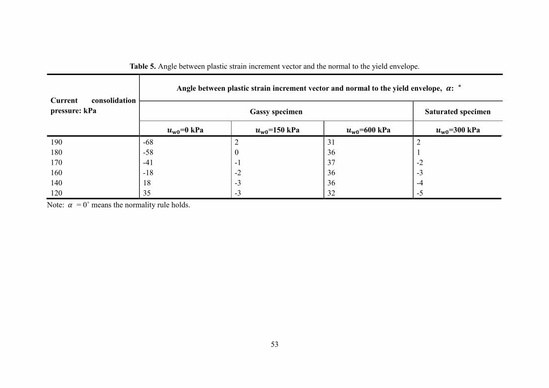
53
Table 5. Angle between plastic strain increment vector and the normal to the yield envelope.
Current consolidation pressure: kPa
Angle between plastic strain increment vector and normal to the yield envelope, 𝜶: °
Gassy specimen Saturated specimen
𝒖𝐰𝟎=0 kPa 𝒖𝐰𝟎=150 kPa 𝒖𝐰𝟎=600 kPa 𝒖𝐰𝟎=300 kPa 190 -68 2 31 2 180 -58 0 36 1 170 -41 -1 37 -2 160 -18 -2 36 -3 140 18 -3 36 -4 120 35 -3 32 -5
Note: 𝛼 = 0˚ means the normality rule holds.
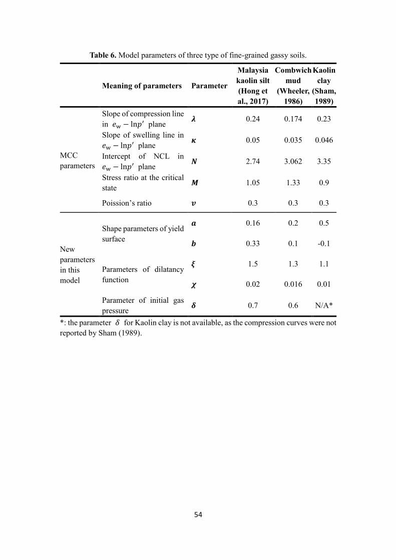
54
Table 6. Model parameters of three type of fine-grained gassy soils.
Meaning of parameters Parameter
Malaysia kaolin silt (Hong et al., 2017)
Combwich mud
(Wheeler, 1986)
Kaolin clay
(Sham, 1989)
MCC parameters
Slope of compression line in 𝑒w − ln𝑝′ plane 𝝀 0.24 0.174 0.23
Slope of swelling line in 𝑒w − ln𝑝′ plane 𝜿 0.05 0.035 0.046
Intercept of NCL in 𝑒w − ln𝑝′ plane 𝑵 2.74 3.062 3.35
Stress ratio at the critical state 𝑴 1.05 1.33 0.9
Poission’s ratio 𝒗 0.3 0.3 0.3
New parameters in this model
Shape parameters of yield surface
𝒂 0.16 0.2 0.5
𝒃 0.33 0.1 -0.1
Parameters of dilatancy function
𝝃 1.5 1.3 1.1
𝝌 0.02 0.016 0.01
Parameter of initial gas pressure 𝜹 0.7 0.6 N/A*
*: the parameter 𝛿 for Kaolin clay is not available, as the compression curves were not reported by Sham (1989).
55
Caption of Figures
Fig. 1. Micro-structure of a typical fine-grained gassy soil (Hong et al., 2019a): (a) micro-computed tomography (μCT) image; (b) scanning electron microscopy (SEM) image.
Fig. 2. The loci of effective stress path due to undrained triaxial compression on gassy Malaysian kaolin (data from Hong et al. 2019b). Fig. 3. (a) A representative volume element (RVE) of fine-grained gassy soil; (b) phase diagram and governing equations for the saturated matrix and gas.
Fig. 4. Varying shapes of yield surface with different values of shape parameter 𝛼 : (a) in 𝑝′ − 𝑞 space; (b) in 𝑝′ − 𝑞 − 𝑒w space. Fig. 5. Identification of the yield point based on different criteria: (a)-(c) deviatoric stress vs axial strain; (e)-(f) dissipated strain energy vs 𝑞 𝑝′⁄ .
Fig. 6. Normalized yield envelopes of gassy Malaysian kaolin (with different 𝑢w0 and ψ0) and incremental plastic strain vectors.
Fig. 7. Comparison between the measured and predicted dilatancy multiplier F for all the tests (in Series I and II).
Fig. 8. Comparison between the measured and predicted shape parameter D for all the tests (in Series I and II).
Fig. 9. Correlating the four new model parameters to the liquid limit (LL) of three types of fine-grained gassy soil.
Fig. 10. Comparison between the predicted and measured compression behavior of (a) gassy Combwich mud (data from Thomas 1987); (b) gassy Malaysia Kaolin silt (data from Hong et al. 2017).

56
Fig. 11. Comparison between the predicted and measured shear behavior of gassy Malaysia Kaolin silt (data from Hong et al. 2019b): (a) stress-strain relation; (b) pore pressure response; (c) effective stress path.
Fig. 12. Comparison between the predicted and measured shear behavior of gassy Combwich mud (data from Wheeler 1986): (a) stress-strain relation; (b) pore pressure response; (c) effective stress path.
Fig. 13. Comparison between the predicted and measured shear behavior of gassy Kaolin clay (data from Sham 1989): (a) stress-strain relation; (b) effective stress path.
Fig. 14. Comparison between the predicted and measured undrained shear strength of gassy Malaysia Kaolin silt (data from Hong et al. 2019b).
Fig. 15. Comparison between the predicted and measured undrained shear strength of gassy Combwich mud (data from Wheeler 1986).
Fig. 16. Comparison between the predicted and measured undrained shear strength of gassy Kaolin clay (data from Sham 1989). Fig. 17. Calculation chart for quantifying the 𝑠u of gassy soils: (a) Malaysia kaolin silt; (b) Combwich mud; (c) Kaolin clay
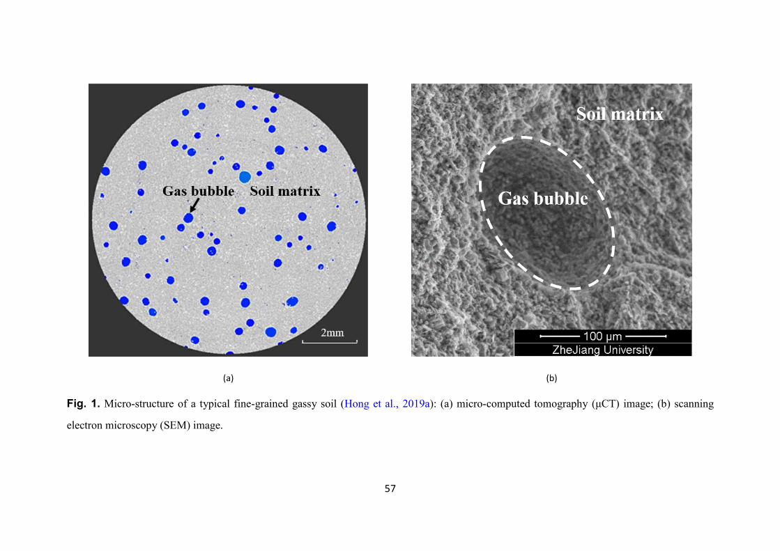
57
(a)
(b)
Fig. 1. Micro-structure of a typical fine-grained gassy soil (Hong et al., 2019a): (a) micro-computed tomography (μCT) image; (b) scanning
electron microscopy (SEM) image.
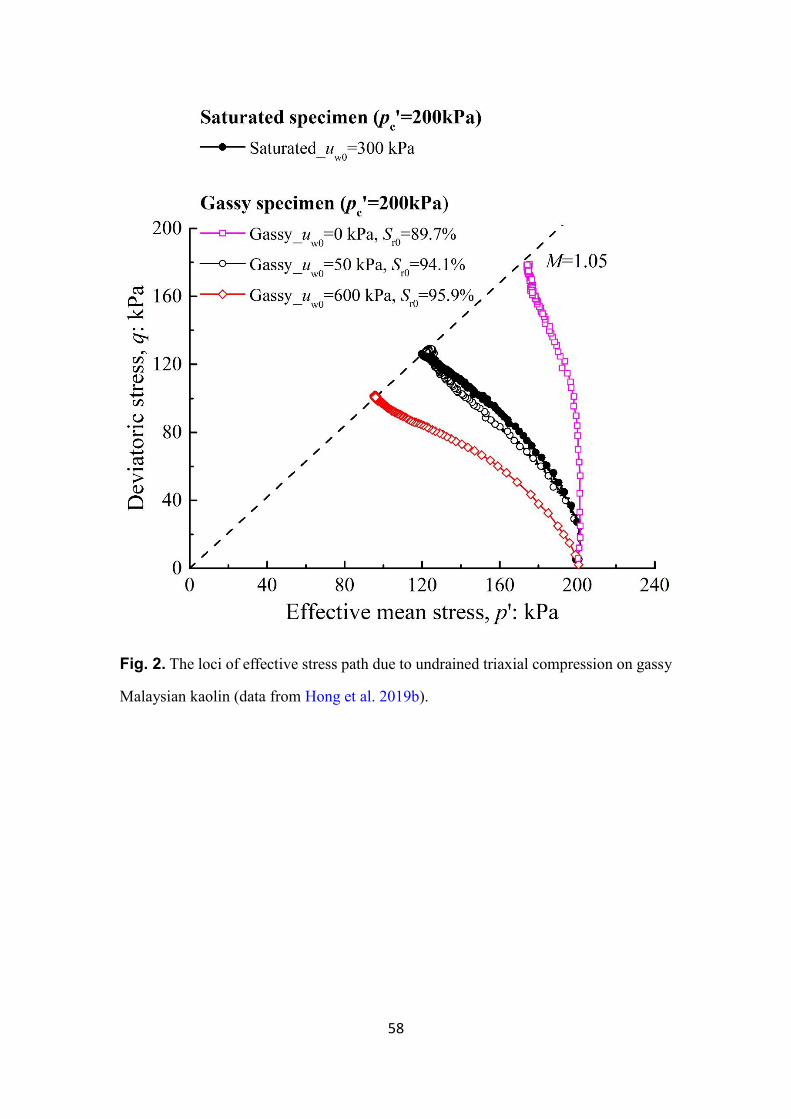
58
Fig. 2. The loci of effective stress path due to undrained triaxial compression on gassy
Malaysian kaolin (data from Hong et al. 2019b).
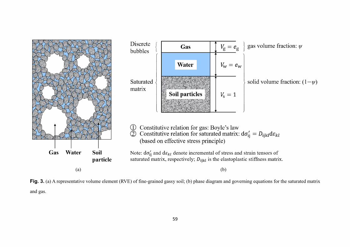
59
(a) (b)
Fig. 3. (a) A representative volume element (RVE) of fine-grained gassy soil; (b) phase diagram and governing equations for the saturated matrix
and gas.
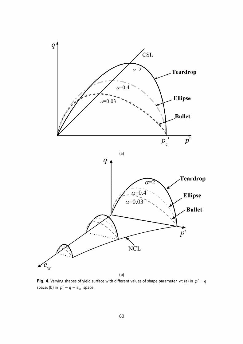
60
(a)
(b)
Fig. 4. Varying shapes of yield surface with different values of shape parameter 𝛼: (a) in 𝑝′ − 𝑞 space; (b) in 𝑝′ − 𝑞 − 𝑒w space.
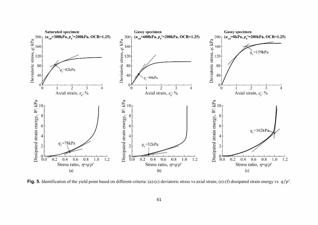
61
(a)
(b)
(c)
Fig. 5. Identification of the yield point based on different criteria: (a)-(c) deviatoric stress vs axial strain; (e)-(f) dissipated strain energy vs 𝑞 𝑝′⁄ .
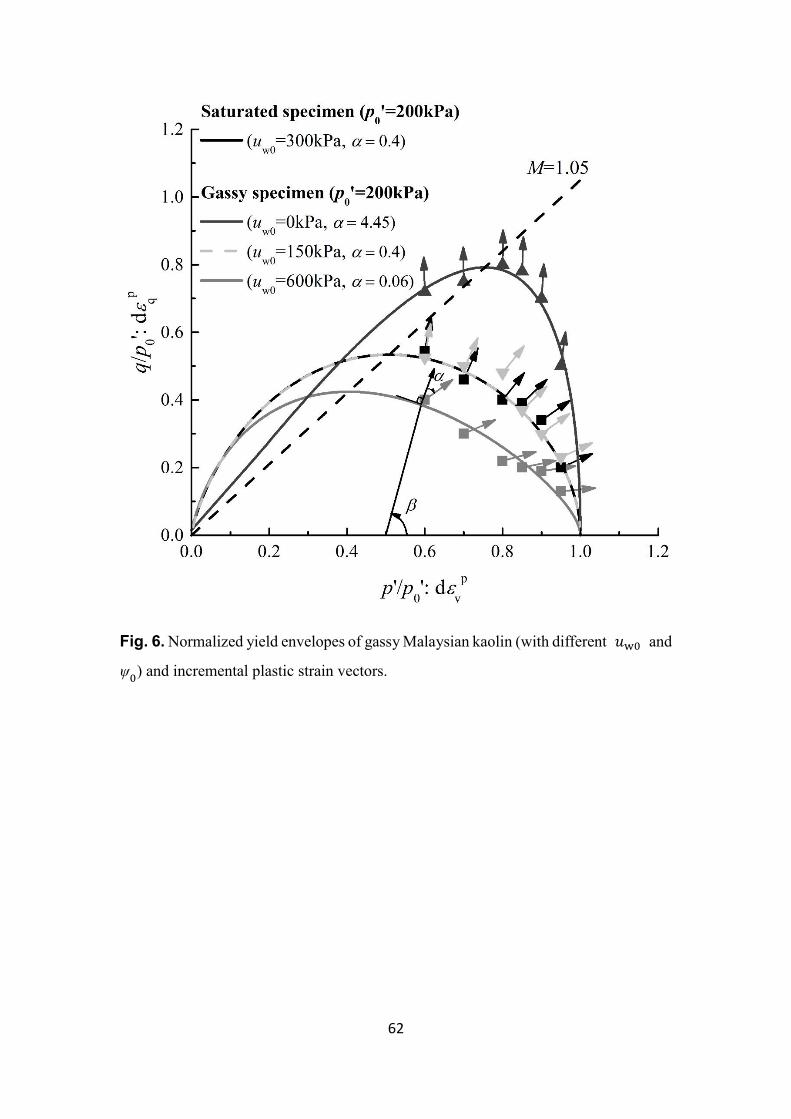
62
Fig. 6. Normalized yield envelopes of gassy Malaysian kaolin (with different 𝑢w0 and
ψ0) and incremental plastic strain vectors.
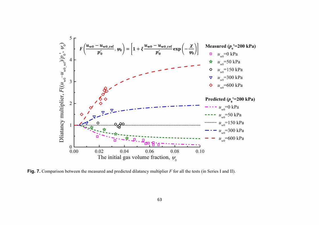
63
Fig. 7. Comparison between the measured and predicted dilatancy multiplier F for all the tests (in Series I and II).

64
Fig. 8. Comparison between the measured and predicted shape parameter D for all the tests (in Series I and II).
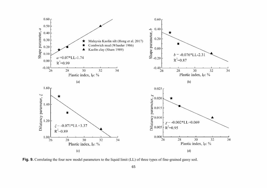
65
(a)
(b)
(c)
(d)
Fig. 9. Correlating the four new model parameters to the liquid limit (LL) of three types of fine-grained gassy soil.
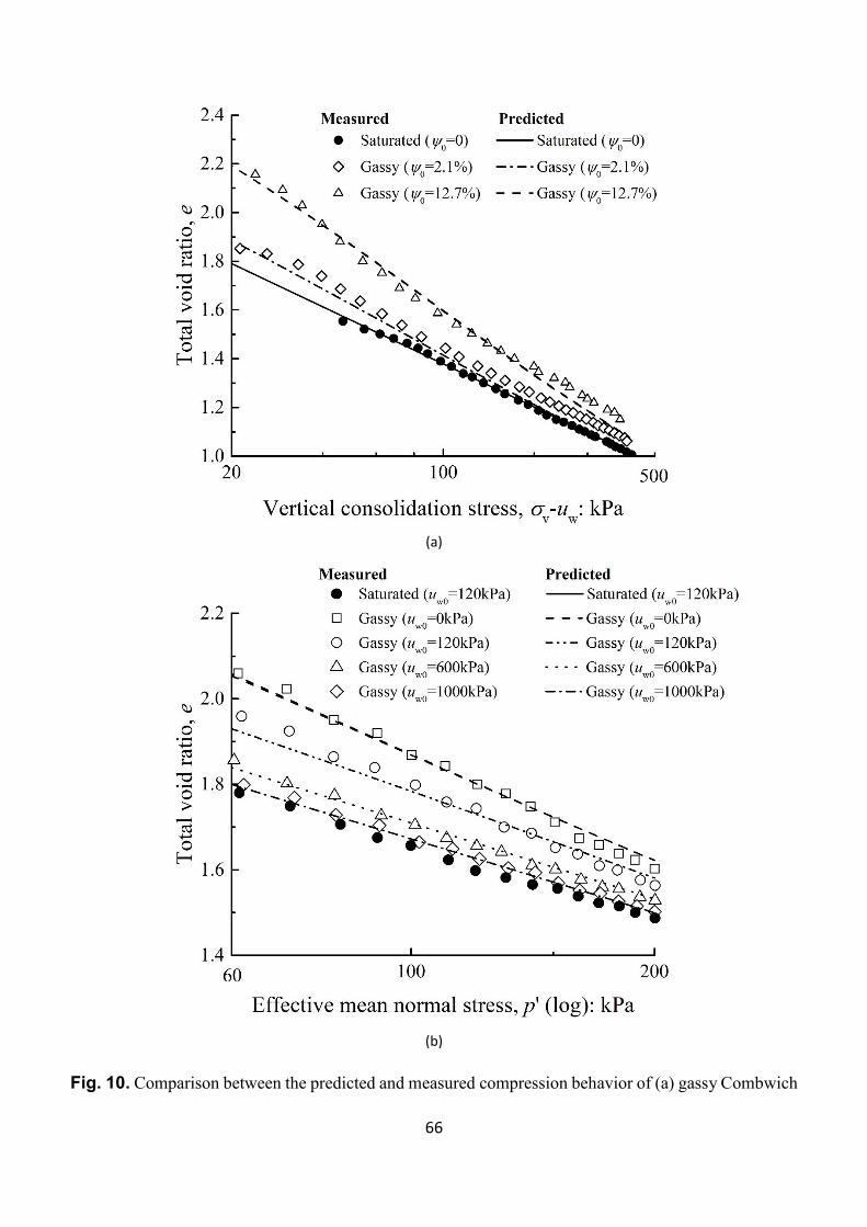
66
(a)
(b)
Fig. 10. Comparison between the predicted and measured compression behavior of (a) gassy Combwich

67
mud (data from Thomas 1987); (b) gassy Malaysia Kaolin silt (data from Hong et al. 2017).
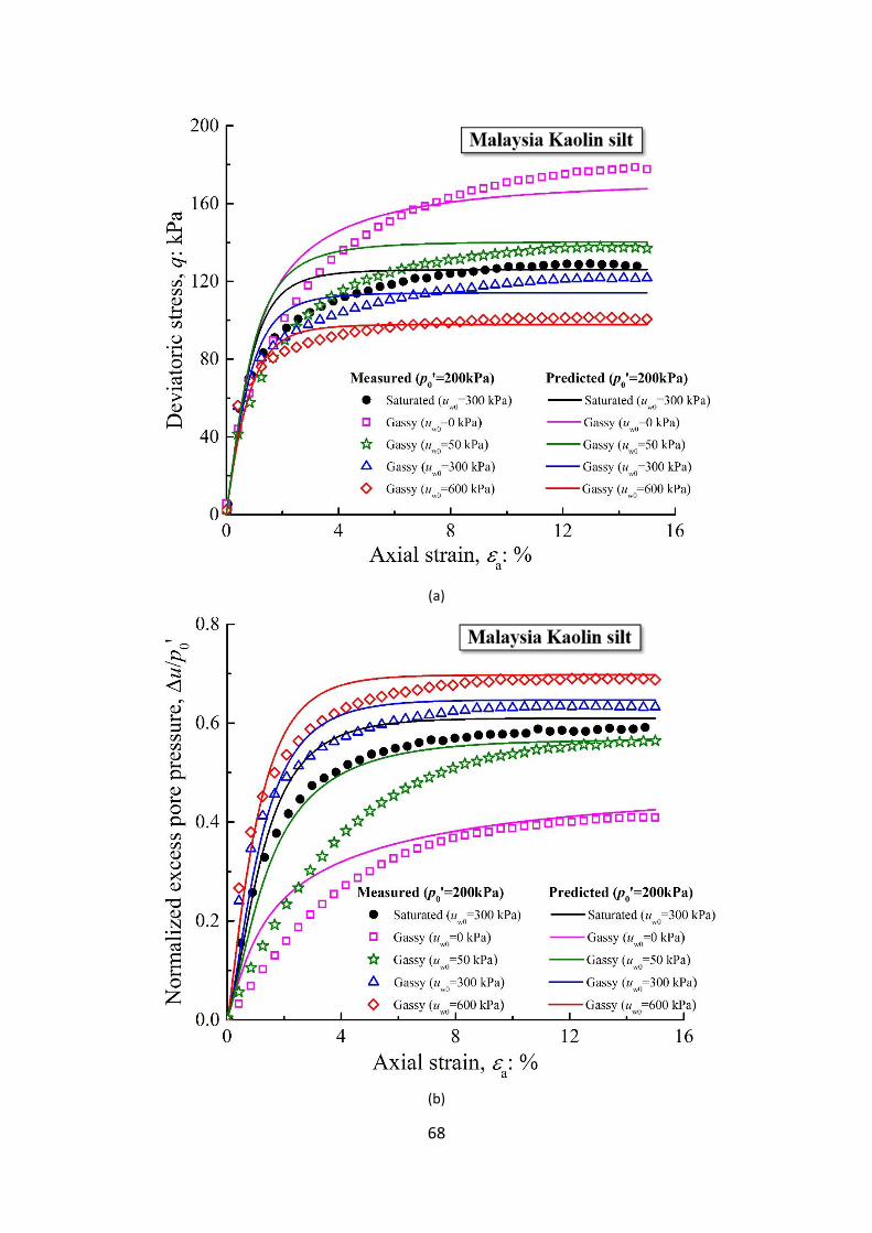
68
(a)
(b)
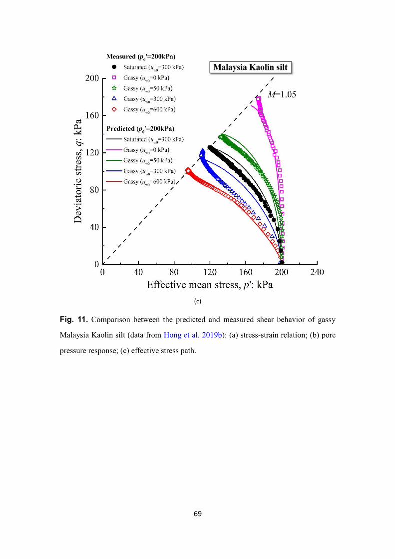
69
(c)
Fig. 11. Comparison between the predicted and measured shear behavior of gassy
Malaysia Kaolin silt (data from Hong et al. 2019b): (a) stress-strain relation; (b) pore
pressure response; (c) effective stress path.
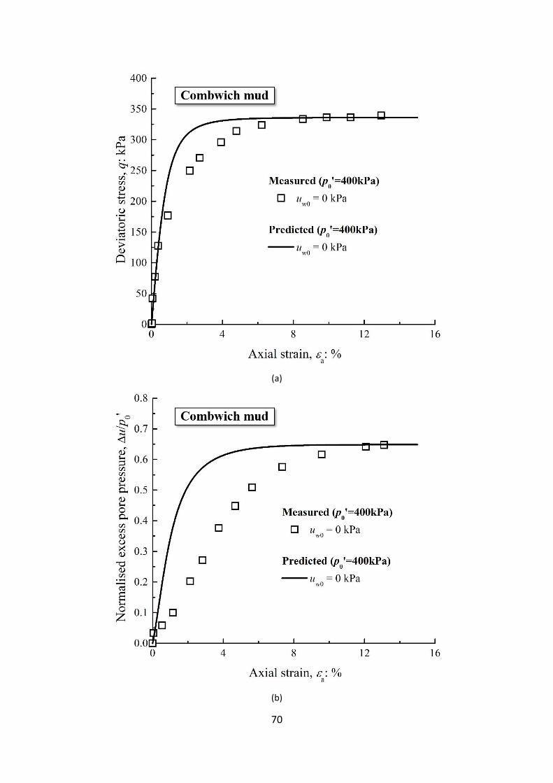
70
(a)
(b)
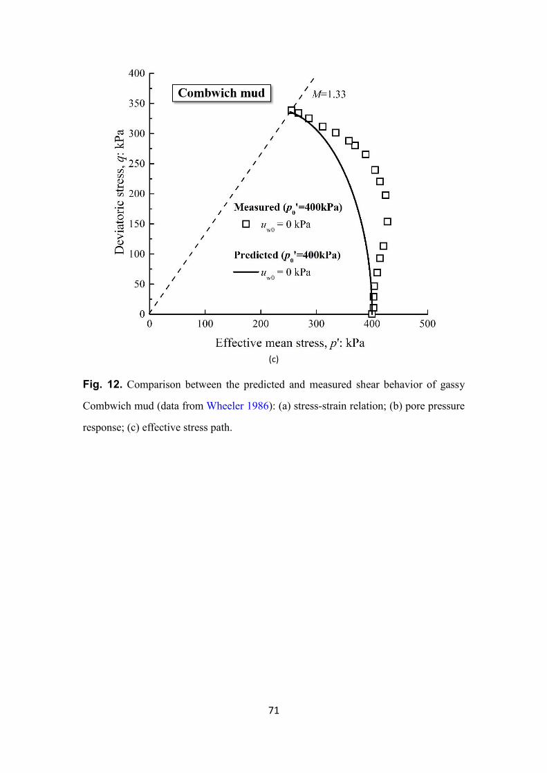
71
(c)
Fig. 12. Comparison between the predicted and measured shear behavior of gassy
Combwich mud (data from Wheeler 1986): (a) stress-strain relation; (b) pore pressure
response; (c) effective stress path.
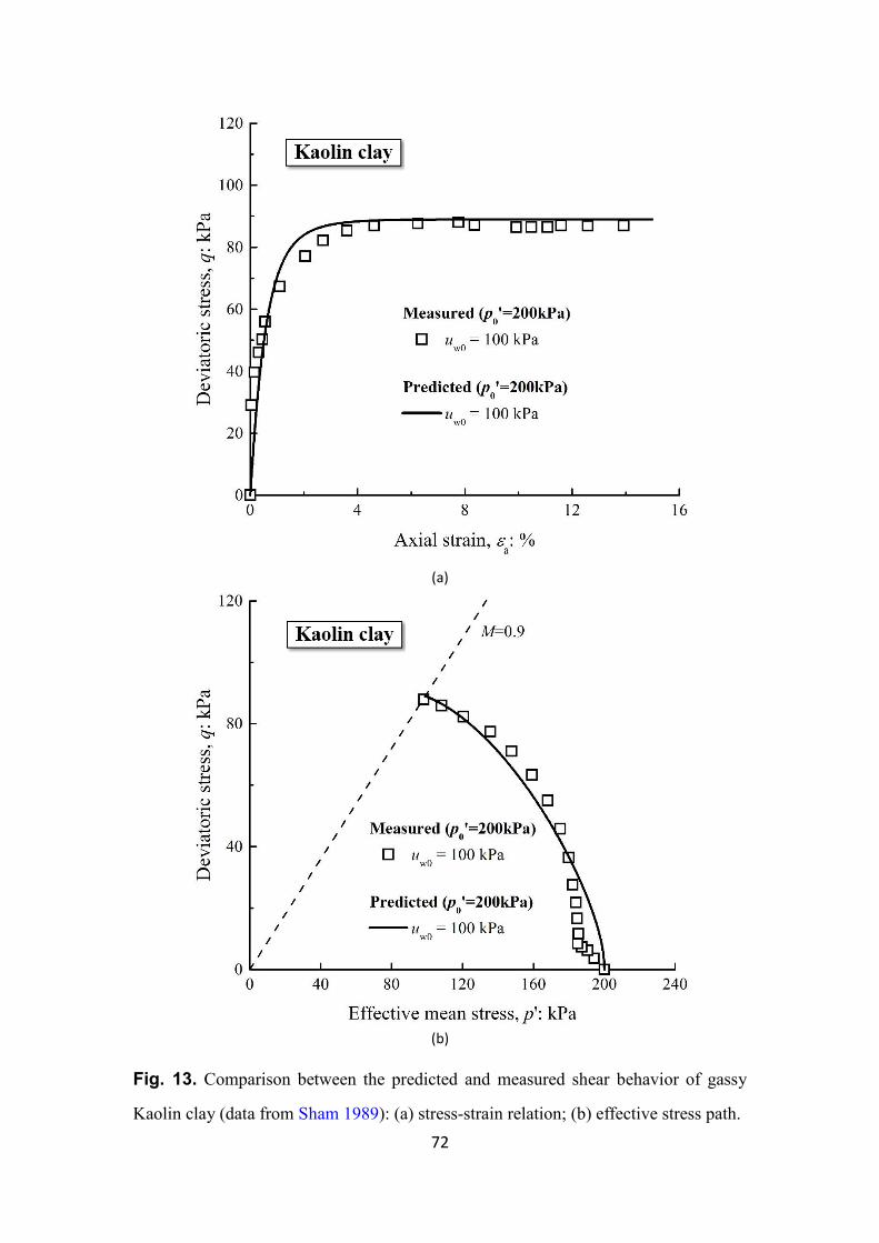
72
(a)
(b)
Fig. 13. Comparison between the predicted and measured shear behavior of gassy
Kaolin clay (data from Sham 1989): (a) stress-strain relation; (b) effective stress path.
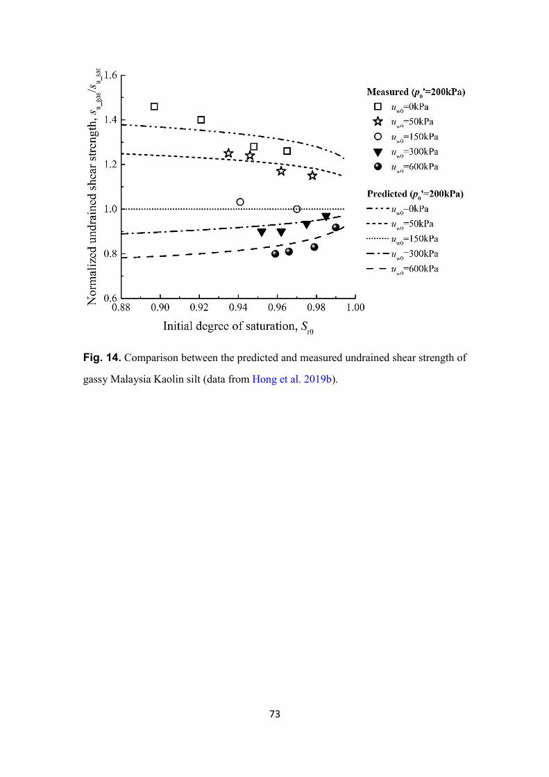
73
Fig. 14. Comparison between the predicted and measured undrained shear strength of
gassy Malaysia Kaolin silt (data from Hong et al. 2019b).
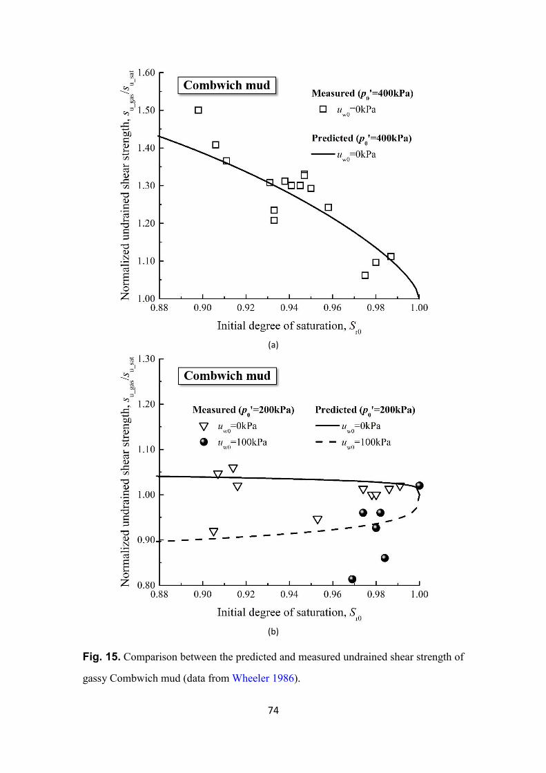
74
(a)
(b)
Fig. 15. Comparison between the predicted and measured undrained shear strength of
gassy Combwich mud (data from Wheeler 1986).
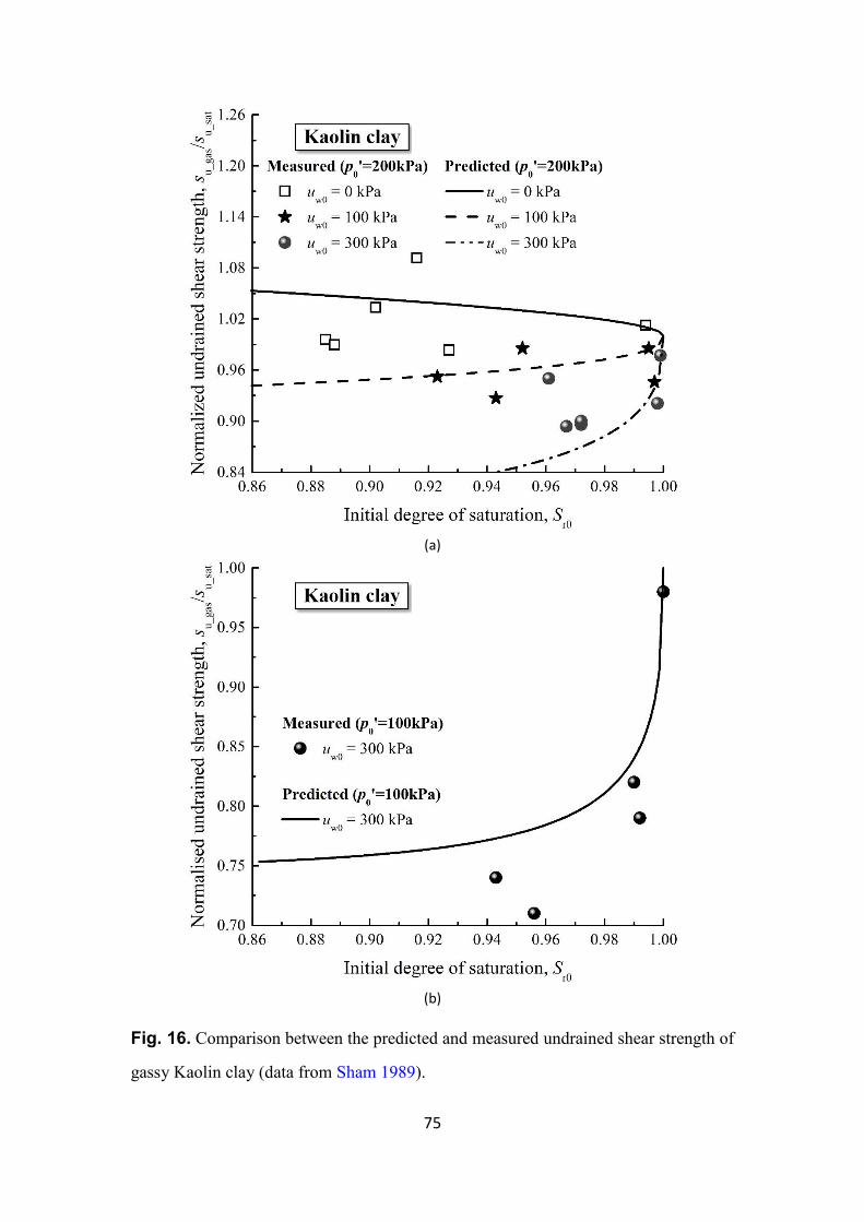
75
(a)
(b)
Fig. 16. Comparison between the predicted and measured undrained shear strength of
gassy Kaolin clay (data from Sham 1989).
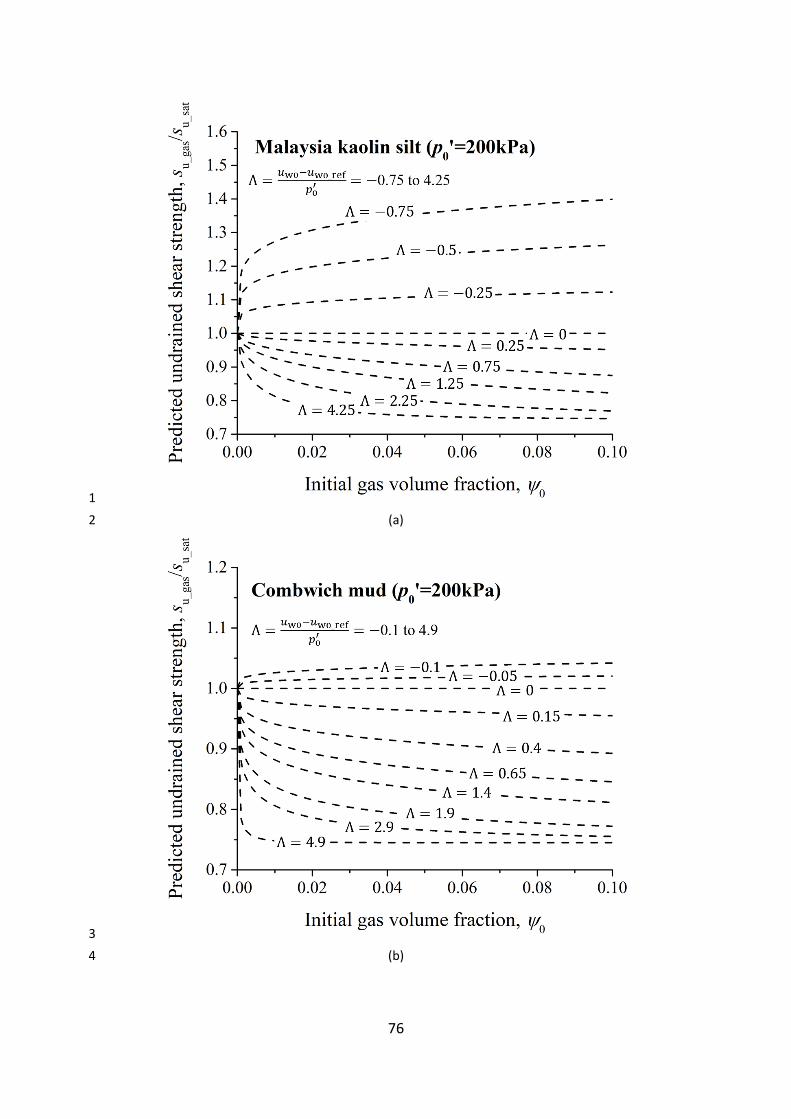
76
1 (a) 2
3 (b) 4

77
5
(c) 6
Fig. 17. Calculation chart for quantifying the 𝑠u of gassy soils: (a) Malaysia kaolin 7
silt; (b) Combwich mud; (c) Kaolin clay. 8
9


