fifth edition lab statistics - ep evaluator...tics, abbott laboratories, sysmex-america and...
TRANSCRIPT

Fifth Edition
Lab StatisticsFun and EasyBy David G. Rhoads
A Practical Approach to Method Validation
Developing Software for the Quality-Driven Clinical Laboratory Since 1983

Lab StatisticsFun and Easy
A Practical Approachto
Method Evaluation
Fifth Edition
byDavid G. Rhoads
David G. Rhoads AssociatesA Data Innovations brand
120 Kimball Ave, Suite 100South Burlington, VT 05403
(800) 786-2622 and (802) 658-1955www.datainnovations.com


Table of Contents -1
Table of ContentsPreface
Copyright Notice ................................................................................................................ iAcknowledgements ............................................................................................................ iPreface for the Fifth Edition ............................................................................................ iiHistory of Our Company ................................................................................................. iiClinical Laboratory and Standards Institute Notice ....................................................iii
Chapter 1Introduction
Chapter 2Effects of Bad Lab Results
Case of the Disappearing Patients ................................................................................2-2Case of the Congressional Hearings .............................................................................2-2Case of the Failed Hospital ...........................................................................................2-2Case of the Mistaken Murder Charge .........................................................................2-3How Lab Error Contributes to Higher Health care Costs .........................................2-3Key Role of Clinical Laboratory .................................................................................2-4Why include these cases in a Lab Statistics Manual? ................................................2-4It’s the Culture, Stupid!! ...............................................................................................2-5
Chapter 3Relevant Highlights of CLIA ‘88 Regulations
Startup Requirements ..................................................................................................3-2Periodic Requirements .................................................................................................3-4Performance Standards .................................................................................................3-5Requirements of Other Deemed Organizations ..........................................................3-5
Chapter 4Statistics 101
Major Statistical Concepts ............................................................................................4-2Statistical Terms used in Clinical Laboratories ..........................................................4-8
-2 Lab Statistics - Fun and Easy
Chapter 5Understanding Error and Performance Standards
Experimental Error ......................................................................................................5-1Concepts of Error ..........................................................................................................5-2Performance Standards (i.e. Total Allowable Error) ..................................................5-5QC Failure ......................................................................................................................5-6Error Profiles ..................................................................................................................5-8Error Budgets .................................................................................................................5-9Calculation of Allowable Systematic Error ............................................................... 5-11Assessing Uncertainty .................................................................................................. 5-11
Chapter 6Defining Performance Standards
Performance Standards Defined...................................................................................6-3Defining PS for Established Methods .........................................................................6-10Comprehensive Approach for Defining PS ................................................................6-10Low End Performance Standards .............................................................................. 6-11Limits defined by Performance Standards ................................................................ 6-11Defining Performance Standards - Case Studies ...................................................... 6-11
Chapter 7Managing Quality Control
Target Mean ..................................................................................................................7-2Target SD .......................................................................................................................7-3QC Rules .........................................................................................................................7-4Tips on Managing QC ..................................................................................................7-5In the Event of QC Failure ............................................................................................7-5Average of Normals .......................................................................................................7-6
Chapter 8Performance Validation Experiments
Startup Requirements ...................................................................................................8-2Recurring Requirements ...............................................................................................8-3Before You Begin. . . .......................................................................................................8-4
Table of Contents -3
Chapter 9Interpreting Method Comparison Experiments
Interpretation of Method Comparison Results ...........................................................9-2Concepts and Definitions ...............................................................................................9-4Types of Method Comparison Experiments ..............................................................9-14Interpretation of Results .............................................................................................9-15Case 1: A Good Example ............................................................................................9-16Properties of Good Data ..............................................................................................9-17Report for Good Case ..................................................................................................9-18Case 2: Effect of Proportional Error..........................................................................9-19Case 3: Effect of Constant Error ...............................................................................9-20Case 4: Effect of Random Error ................................................................................9-20Case 5: Non-Linear Pattern .......................................................................................9-23Case 6: Effect of Outliers ...........................................................................................9-24Case 7: Effect of Extreme Range ...............................................................................9-25Case 8: Effect of Range of Results .............................................................................9-26Case 9: Effect of Number of Specimens ....................................................................9-28Case 10: Effect of Poor Distribution of Results ........................................................9-29 Method Harmonization Experiment .........................................................................9-30
Chapter 10Interpreting Linearity Experiments
Definition of Some Statistical Terms ..........................................................................10-2Linearity ......................................................................................................................10-2Accuracy .......................................................................................................................10-5Reportable Range ........................................................................................................10-7Calibration Verification ...............................................................................................10-8Case Studies ..................................................................................................................10-8Case 1: A Non-Linear Case .........................................................................................10-9Case 2: Inaccurate Results ........................................................................................10-10Case 3: Failures Due to Inappropriate Specifications ............................................ 10-11

-4 Lab Statistics - Fun and Easy
Chapter 11Understanding Proficiency Testing
Regulatory Requirements ........................................................................................... 11-1Theoretical Approach .................................................................................................. 11-2Bias ................................................................................................................................ 11-3Calculating the Probability of PT Failure ................................................................. 11-4Statistics ........................................................................................................................ 11-7Strategy to Pass Proficiency Testing ........................................................................... 11-9Proficiency Testing Report ........................................................................................ 11-11
Chapter 12Precision Experiments
Simple Precision Experiment ......................................................................................12-2Simple Precision Report (Page 1) ...............................................................................12-3Complex Precision Experiment ..................................................................................12-4Complex Precision Report (Page 1) ...........................................................................12-5Complex Precision Report (Page 2) ...........................................................................12-6
Chapter 13Understanding Reference Intervals
Key Concepts ................................................................................................................13-1Sources of Medical Decision Points ............................................................................13-2Verifying vs. Establishing vs. Neither ........................................................................13-3Verifying a Normal Range .......................................................................................13-3Establishing a Normal Range .....................................................................................13-5MDP’s which are “Cast in Stone” ..............................................................................13-7Outliers .........................................................................................................................13-8Accuracy and Precision for Normal Ranges .............................................................13-9Interpreting the Reference Interval Report ............................................................13-10Case 1: An Uncomplicated Example .......................................................................13-15Case 2: Skewed Data ................................................................................................13-16Case 3: Effect of Number of Specimens ...................................................................13-17Case 4: Partitioning (by Gender, Race, etc.) ...........................................................13-19Case 5: Effect of Outliers ..........................................................................................13-20Case 6: Effect of Tails ................................................................................................13-22ERI Report showing Effect of Tails (no Truncation) ..............................................13-25ERI Report showing Effect of Tails (with Truncation)...........................................13-26
Table of Contents -5
Chapter 14Sensitivity Experiments
Sensitivity (Limits of Blank) Experiment .................................................................14-2Sensitivity (LOB) - Alternate Experiment .................................................................14-3Sensitivity (Limits of Quantitation) Experiment ......................................................14-3
Appendix APublished Performance Standards
Medical Requirements ..................................................................................................A-4
Appendix BTechnical CLIA ‘88 Regulations
Subpart K - Quality Systems for Nonwaived Testing .............................................. B-1Selected Interpretative Guidelines ............................................................................ B-17
Appendix CGlossary
AppendixDBibliography
Appendix E Our Products
EP Evaluator®, Release 10........................................................................................... E-1Instrument Manager®.................................................................................................. E-5

-6 Lab Statistics - Fun and Easy

Preface -i
Preface
Copyright Notice
This manual is copyrighted 1996 - 2012 by Data Innovations, LLC. All rights are reserved worldwide. No part of this book may be reproduced, transmitted, tran-scribed or translated into any language by any means without the express written consent of Data Innovations, LLC.
For further information, contact:
David G. Rhoads AssociatesA Data Innovations brandee.datainnovations.com
DATA INNOVATIONS NORTH AMERICAPhone: (802) 658-1955Fax: (802) 658-2782Email: [email protected]:
DATA INNOVATIONS EUROPEPhone: +32 2 332 24 13Fax: +32 2 376 43 84Email: [email protected]
DATA INNOVATIONS ASIAPhone: +852 2398 3182Fax: +852 2398 8667Email: [email protected]
DATA INNOVATIONS LATIN AMERICAPhone: +55 (11) 3801-3283Fax: +55 (11) 3871-9592Email: [email protected]

-ii Lab Statistics - Fun and Easy
Acknowledgements
My wife, Elizabeth A.L. Rhoads, has as always, been very helpful in the produc-tion of this book. She remains a tower of support.
My colleague, Marilyn Fleming, has been essential to the development of EP Evaluator®. Her background in programming and statistics coupled with a will-ingness to understand major components of how a laboratory works has been an essential component of the success of our company and our software. In recent years, Marilyn has been presenting several sections of our workshop including one section on statistics. Her input has been invaluable.
Gregory R. Vail and David G. Potter, founders of Data Innovations. They deserve recognition both for their vision that quality in clinical laboratories is important, and for their commitment to help laboratories achieve that quality.
If you, the reader, have comments or criticism about this book, please share them with us. In that way, we will be able to improve the next version.
I take full responsibility for any errors in this book.
David G. Rhoads, Ph.D., DABCC Kennett Square, PA October, 2009
Preface for the Fifth Edition
There is one notable difference between the Fourth and Fifth editions of Lab Statistices Fun and Easy: the Performance Standard for HbA1c was changed to reflect current requirements (see Table I on page 6-4).
The changes between the Third and Fourth editions were relatively few, but of major consequence. Their genesis was the changes that we have made in the pre-sentations for our workshops. This book now better reflects those changes which were made as part of our process to improve the presentation of clinical labora-tory statistics.

Preface -iii
History of Our Company
The firm, David G. Rhoads Associates, Inc. (Rhoads) which initially developed EE was incorporated in 1983. It was always deeply involved in the science and technology of the clinical laboratory. This has evolved over the years to include quality assurance and lab management tools.
David G. Rhoads is the individual primarily responsible for the overall design of EE. He has had 9 years of experience as a hospital based clinical chemist. He has a Ph.D. in Biochemistry from Brandeis University, is Board Certified in Clinical Chemistry (DABCC) and has been a member of the AACC since 1975. He is very concerned with the quality of the work coming from clinical laboratories.
Data Innovations (DI) acquired Rhoads in July, 2009. DI was incorporated in 1989 by Gregory R. Vail and David G. Potter. Its primary product is middleware (MW). MW is a laboratory data management software application designed to increase efficiencies and improve workflow. MW supports pre-analytical, analyti-cal, and post-analytical sample processing and non analytical tasks such as equip-ment maintenance.
Data Innovations is the leading vendor of MW world-wide having installed over 6500 systems in over 60 counties. EP Evaluator® is the leading statistical qual-ity assurance software package and is in use in well over 2000 labs in the United States and Canada.
Our customers and partners include large IVD vendors such as Roche Diagnos-tics, Abbott Laboratories, Sysmex-America and Beckman-Coulter; reference labs including Quest Diagnostics, and LabCorp plus many hospitals and medical centers, large and small throughout the world.
Clinical Laboratory and Standards Institute Notice
This software incorporates copyrighted Standards and/or Guidelines of the Clini-cal and Laboratory Standards Institute (“CLSI”). These Standards and/or Guide-lines are used in this software by permission of CLSI.
CLSI HEREBY DISCLAIMS ANY AND ALL LIABILITY TO ANY USER OF THIS SOFTWARE.
For updates of the Standards and/or Guidelines incorporated into this software and for information about other CLSI publications, the user may write to CLSI at 940 West Valley Road, Suite 1400, Wayne, PA 19087-1898, may call 610-688-0100, may e-mail CLSI at [email protected], or may send a fax to 610-688-0700.

-iv Lab Statistics - Fun and Easy

Introduction 1-1
C h a p t e r
1Introduction
Our point, which we will proceed to demonstrate to you, is that field of Clinical Laboratory Statistics as we enter the 21st Century is not rocket science.
We will discuss in a systematic, easily understandable manner what clinical laboratory personnel need to know to keep their laboratories in compliance with requirements of CLIA ‘88 and other regulatory agencies for method validation, calibration verification and method comparison.
The items to be discussed include: • Cases of real lab disasters!!• CLIA ‘88 technical regulations. • Statistical concepts relevant to CLIA ‘88 and method validation. • Concepts of error and how they relate to method validation.• The process of establishing performance standards.• General approaches to managing quality control.• Design and interpretation of linearity style experiments.• Design and interpretation of precision experiments.• Design and interpretation of method comparison experiments.• Design and interpretation of reference interval experiments.• Design and interpretation of sensitivity experiments.We make the assumption throughout that the user has software which performs these various calculations. Therefore we will not discuss the mathematics and algebra of statistics. Our examples are based on the EP Evaluator®, Release 10, a program developed and marketed by Data Innovations, LLC, and used widely in the clinical laboratory community by hospital labs, reference labs and vendors.

1-2 Lab Statistics - Fun and Easy

Effects of Bad Lab Results 2-1
C h a p t e r
2Effects of Bad Lab Results
In This ChapterPoor quality assurance practices in the clinical laboratory can cause real trouble. We discuss:• A number of real cases which have ranged from merely expensive to disas-
trous.• An estimate of how much poor QC practices can cost.
Many people assume that as long as a lab continues to pass its proficiency testing, there will be no problems. Not true!! Not only can there be negative effects with respect to patient care, but also with respect to the laboratory and hospital. Here are several real cases which demonstrate real problems that can occur when labs produce erroneous results. In all these cases, the laboratory passed proficiency testing. These documented cases resulted in:• Patient death• Hospital failure• Loss of business• Loss of management jobs• Higher costs for the health care system• Lawsuits against the laboratory

2-2 Lab Statistics - Fun and Easy
Case of the Disappearing Patients
I visited one lab in 2004 which observed that its referring physicians were sending their patients to the other hospital in town. On investigation, they found that this was happening because its own results were so bad.
It turns out that this lab was defining its target SD values for the chemistry elec-trolytes using the mean SD from the BioRad QC results. The reason this is a prob-lem is that the mean SD is calculated across all the available SD’s. Consequently it will be 2-3 times what an appropriate value should be.
Case of the Congressional Hearings
A whistle-blower reported a long series of quality assurance problems at the Maryland General Hospital in Baltimore, MD in 2004. The ones that got most attention had to do with performance of HIV and HBsAg tests. The instrument on which those tests were performed had a long history of maintenance problems which the vendor was unable to resolve even after numerous service calls. (Hospi-tal and lab management had been ignoring many QA issues.)
As soon as the University of Maryland Medical System realized that it had a prob-lem, to its credit, it immediately replaced senior management both for the hospital and for the laboratory. In other words, several people lost their jobs because the laboratory for which they were responsible had such a poor quality assurance record. (Baltimore Sun - 2004)
The laboratory then attempted to re-test the approximately 1500 patients previ-ously tested. It was able to find 460 of the patients on which the HIV testing was done during this period and repeated the test at no charge to the patient. The CEO who was testifying before the Congressional Subcommittee proudly announced that 99.6% of the results were the same as before.
If you do the math, you will find that two patients changed. The results for one of those patients changed from HIV positive to HIV negative. That patient has sued Maryland General for $5,000,000.
Case of the Failed Hospital
At St. Agnes Medical Center in Philadelphia, 3 patients died from inaccurate he-mostasis results in 2001. These deaths got national attention. The hospital closed in 2004. While the hospital failure was probably not solely a result of these labo-ratory issues, it must have been a significant factor.

Effects of Bad Lab Results 2-3
Case of the Mistaken Murder Charge
A disabled girl died in July, 2004. During the autopsy process, blood specimens were submitted to a lab for analysis. The lab determined that the specimen had lethal levels of phenobarbital. This was reported to local law enforcement. Conse-quently, the authorities jailed the child’s mother for First Degree Murder. (Mielc-zarek - 2004)
The specimen was rechecked by the lab and again the concentration of the drug was found to be lethal. Later the specimen was sent to other labs and was found to be in the therapeutic range. At that point 3 months after the initial indictment, the charges against the mother were dropped. Potential consequences for the lab include revocation of its license to operate as well as a lawsuit brought by the child’s mother.
How Lab Error Contributes to Higher Health Care Costs
If lab results causing incorrect diagnoses amounted to 0.12% of the results for a lab producing 1 million tests a year, that would mean 1,200 patients per year would be incorrectly diagnosed (i.e. about 3.5 per day).
Plebani and Carraro (1997) reported 49 medically significant errors from 40,490 tests (0.12%). A medically significant error is one which resulted in inappropriate care or evaluation of a patient. Ref: CCJ (1997)
If the average additional cost for each of these incorrectly diagnosed patients was only $1,000, then these incorrect results would result in an additional $1.2 million cost per year for the health care system.
This cost is 40% of the total budget for a lab performing this volume of work. The annual budget for a lab this size is approximately $3 million.
One important observation is that if the lab makes a mistake, with few exceptions, the costs of that mistake are not paid by the laboratory, but instead by some other cost center. In other words, as far as the lab is concerned, these errors are silent and lab personnel are usually not aware of the errors or costs that arise from their work.

2-4 Lab Statistics - Fun and Easy
Key Role of Clinical Laboratory
Sometimes I get the feeling that laboratory workers don’t really appreciate the importance of their work. Consider the following:• Clinical laboratory costs are 3-4% of the total U.S. health-care budget.• At Mayo Clinic, 94% of the objective data in patients’ charts were from the
laboratory. Forsman - 2004)• Lab data leverages 60-70% of all critical decisions. (Forsman - 1996)In other words, while we are but a small component of the total health care system, our data control a large majority of the critical decisions.This is hardly the role of an unimportant component of the health case system!
Why include these cases in a Lab Statistics Manual?
These cases have been included so that the readers of this book will have some resources so they can make the case to their management that these problems can and do happen. While they may seem infrequent, they happen often enough so they are a very real problem.

Effects of Bad Lab Results 2-5
It’s the Culture, Stupid!!
On two trips in 2004 and 2005, one airline lost my baggage. Consequently, I had to give my workshops in my travelling clothes and had to do without some ma-terials. On one of these trips, I was rather upset. It seemed to take a major effort on my part to get my luggage back. Fortunately in both cases, my luggage was delivered the next day.
I have had many other trips on this airline in which my baggage was not lost. Perhaps we could say that I have 95% confidence that my luggage would be avail-able for pickup at my destination. By implication then, for 5% of my trips on this airline, my luggage will be lost. That is not a happy prospect.
Could it be that this airline has a culture which accepts this degree of failure?
Similarly, one can argue that laboratories have a culture which accepts failure. The QC rules are designed so that some failure is acceptable. Witness the 2-2s rule which says that failure occurs when 2 consecutive QC results are outside the 2 SD limits. If at least one result is inside the limits, the process is officially in control. One common approach in dealing with this event with 2 of 2 results outside the limits is to repeat both QC specimens. If during the second analysis, at least one result is acceptable, then of course one can accept the run and the prob-lem has gone away at least for the moment.
The fundamental problem is that we have to decide which of the many failure conditions are not acceptable. This problem is compounded by the fact that in the stressful world of the clinical laboratory, it is easier (and often within the rules) to ignore problems than it is to fix them. The obvious answer is to define a culture in which failure is unacceptable. This of course, is much easier said than done. Laboratory practices, including statistics, over the last half century have established the attitude that some failure is accept-able. Perhaps in the next half century, our industry can devise a series of practices such that failure conditions can be readily detected and hence eliminated.
In the meantime, we need to modify our present practices to do two things:• Define a reasonable set of performance goals.• Strive to minimize failure in the process of achieving these goals.The remainder of this book will discuss some of the regulatory and statistical aspects to doing just that.

2-6 Lab Statistics - Fun and Easy

Relevant Highlights of CLIA ‘88 Regulations 3-1
C h a p t e r
3Relevant Highlights of
CLIA ‘88 Regulations
In This ChapterCLIA ‘88 technical regulations define tasks which laboratories are required to do as part of their quality assurance and quality control program. We discuss:• The groups of clinical laboratory methods and which tests are included in each
group.• The tasks required to validate new methods.• The tasks required to validate methods on a recurring (semi-annual) basis.• Specifies how performance standards (specifications) are to be used.
The regulatory environment was promulgated in the Clinical Laboratory Improve-ment Amendment of 1988 (CLIA ‘88). This act of Congress was stimulated by several scandals relating to PAP smears which received national publicity in the Wall Street Journal.
Complete sections of the relevant technical requirements in the “Final Rule” are in Appendix B of this manual.
There are two types of technical requirements: a) those that must be done before results are reported for a new method (Startup); and b) those that must be done periodically, at least semi-annually (Periodic).
3-2 Lab Statistics - Fun and Easy
Startup Requirements
This group of regulations describe what laboratories must do prior to reporting patient test results.
The methods have been divided into five major groups:
Waived methods: These are methods which are so simple that no one in their right mind can screw up the results. Some of these methods are sold over the counter in drug stores. The federal government has reviewed each of these methods and has waived them. This class of method will not be discussed further in this book.
Physician Performed Microscopy: A concession to the physician’s lobby. This covers procedures performed by a physician with his microscope. This calls of methods will not be discussed further in this book.
Unmodified methods: These are methods adopted by a laboratory which are “un-modified, FDA-cleared or approved test systems.”
Modified methods: These are methods adopted by a laboratory which either are “home-brew” methods or are modified versions of approved methods.
The CAP has taken the position that treats all methods as “Modified Methods”. For those labs inspected by the CAP, then regulations pertaining to the Modified Methods pertain.
Unmodified methods
The regulations [493.1253(b)(1)] for the methods cleared by the FDA are very clear. They provide that the laboratory must “demonstrate that it can obtain per-formance specifications comparable to those established by the manufacturer for “accuracy, precision and reportable range.”” The lab must also “verify that the manufacturer’s reference intervals (normal values) are appropriate for the labo-ratory’s patient population.” Modified methods
The requirements for “everything else” are significantly more rigorous [493.1213(b)(2)]. Prior to reporting patient test results, a laboratory must estab-lish for each method, performance specifications as listed below: Must be demonstrated using an experiment. Accuracy Precision Reportable range of patient test results Reference range(s) Sensitivity (e.g. the lowest result which can be reported)May be documented in laboratory procedure manual. Specificity (interfering substances).

Relevant Highlights of CLIA ‘88 Regulations 3-3
Important Validation Issues
There was a major change in the initial validation requirements between the first set of regulations published in 1992 and this set in 2003. In the first set, the validation process could be as the manufacturer specified. One result of this was that for many instruments, there was no rigorous establishment of accuracy and reportable range.
The second set of regulations specifies clearly that validation of the set of instru-ment performance parameters must be done in all cases for both modified and unmodified methods. This is a significant change for hematology instruments for which a method comparison experiment was all that was done in most cases to satisfy accuracy and reportable range requirements.
Another issue is that while many vendors verify the instrument or method for their customer, usually that service only takes the form of demonstrating accuracy, precision and reportable range. They usually do not verify the reference interval. This means that it is up to the individual labs to verify or establish their reference intervals.
Verification of reference intervals can be done two ways: (1) either with an explic-it reference interval experiment (establish or verify), or (2) to perform a method comparison experiment to demonstrate that there is no difference in the medical decision points from the previous method. I know that very few labs do the ex-periments to establish therapeutic ranges for drugs or do the experiments to (re-)establish medical decision points for analytes such as PSA (where the traditional cutoff is 4 ng/mL and no “normal range” is published).

3-4 Lab Statistics - Fun and Easy
Periodic Requirements
Two recurring technical requirements for laboratories are calibration verification and demonstration of the comparability of multiple methods or instruments used for obtaining results on the same analyte. Calibration Verification (CalVer) is now the same experiment as the CAP’s Verification of AMR (Analyte Measurement Range).
Calibration Verification
CalVer “is required to substantiate the continual accuracy. . . throughout the labo-ratory’s reportable range of test results for the test system.” CalVer must be done as follows:• Following manufacturer’s CalVer instructions.• Using criteria specified by the laboratory. Materials must include specimens
with a minimal or zero value, a mid-range value and a maximum value near the upper limit of the reportable range respectively.
• Frequency of performance of CalVer is:• At least every six months or whenever one of the following occurs:
• A complete change of reagents occurs unless the laboratory can demon-strate that no changes in the analytical system have occurred.
• There is major preventative maintenance or replacement of critical parts which may affect instrument performance.
• Control materials reflect an unusual trend or shift, or are outside of the laboratory’s acceptable limits, and other means of assessing and correct-ing unacceptable control values fail to identify and correct the problem.
• “The laboratory’s established schedule for verifying the reportable range for patient test results requires more frequent calibration verifica-tion.”
• All calibration and CalVer procedures must be documented.
Exceptions to the Requirements for Calibration and CalVer Details are listed in the CMS Interpretative Guidelines (2003) and are quoted in part in “Selected Interpretative Guidelines” on page B-17.
Comparison and Accuracy of Test Results
The laboratory must demonstrate that all the results for the same test in the same LIS environment are statistically identical across all instruments.
If a laboratory performs tests not among the 75 analytes for which proficiency testing is required, the laboratory must have a system for verifying the accuracy of its test results at least twice a year. [493.1281]

Relevant Highlights of CLIA ‘88 Regulations 3-5
Performance Standards
Laboratories must establish or verify Performance Standards for each test. They may get these either from the manufacturer (for unmodified methods) or establish them (for modified methods) (Section 493.1253(b)(3)). These performance stan-dards are to be used for calibration and calibration verification.
Furthermore laboratories are required to make these same performance standards available to clients upon request. (493.1291(3)).
Requirements of Other Deemed Organizations
College of American Pathologists (CAP) is one of several organizations which has deemed status which can inspect and accredit clinical laboratories. Some of the others include JCAHO (Joint Commission for Accrediting Health Organizations), COLA (used primarily by POLs), as well as several states including New York State.
While the inspection process varies significantly across these organizations, all the organizations must meet or exceed the requirements specified in CLIA ‘88. The details of the inspection process vary substantially depending on the organization performing the inspection. Each of these organizations has its own checklist of requirements. Of these checklists, perhaps the CAP’s is most rigorous. The fol-lowing table compares the requirements of CLIA ‘88 and CAP.
Comparison of CLIA ‘88 and CAPMethod Evaluation Requirements
CLIA ‘88 CAPAccuracy Required RequiredLinearity RequiredReportable Range Required RequiredPrecision Required RequiredReference Interval Required RequiredMethod Comparison RequiredSensitivity Conditionally Required RequiredSpecificity Conditionally Required OptionalCarryover RequiredRequired means that the experiment is required in at least one accreditation checklist.

3-6 Lab Statistics - Fun and Easy
Statistics 101 4-1
C h a p t e r
4Statistics 101
In This ChapterStatistics are the lifeblood of quality assurance in the clinical laboratory. We discuss:
• Purpose and philosophy of statistics in the clinical laboratory.• Lists of major statistical measures.• Concepts of central tendency and dispersion.• Significance of various degrees of dispersion.• Criteria for detection and elimination of outliers.• Definitions of statistical terms used in clinical laboratories.
“There are lies, damn lies and statistics.”Mark Twain
Statistics can be either enlightening or bedeviling depending on the quality of the results and way they are presented.
One of the great dangers of statistics is that they can be used to distort or conceal the realities of a situation. Politicians often do this deliberately. Laboratorians often do this because of their ignorance of how a given situation is best described statistically. Our effort in this book will be to describe the uses of statistics and error with respect to: • Understanding how error concepts describe the performance of clinical labo-
ratory methods.• Understanding the basis for performance standards.• Understanding how performance standards are established.• Evaluating clinical laboratory methods with respect to performance standards.
First, we must understand the basic concepts of statistics because they are used to describe the reality of clinical laboratory tests, namely uncertainty and error. Only after we have learned the relationship of statistics to error and uncertainty can we understand how to correctly evaluate, describe or establish appropriate perfor-mance of a method.

4-2 Lab Statistics - Fun and Easy
Statistics are useful because they allow us to predict future performance to a specified probability. We can predict the range within which results are expected from a series of events. However, predicting the exact outcome of an event is like hitting the lottery - pure luck.
For example, we can reliably predict that the values we obtain from repeated as-say of a specimen for LDH will be in the range of 31 and 39. We cannot predict with any degree of assurance that the first specimen will have a value of 38 and the second a value of 36.
Note: Statistics are meaningful only in context.
Fact: John Kruk, first baseman for the 1993 Philadelphia Phillies, mad an out 66% of the times he came to bat.
This would seem to be terrible performance with failure two-thirds of the time. Certainly it would be terrible for a professional basketball player shooting foul shots (typically 20 to 30% failure). However, if you put this in context of what other players have achieved, Kruk had a wonderful season. The 66% figure corre-sponds to a batting average of 0.340. He was in the top 3 percentile of hitters that year. Typical team batting averages are about 0.270. It is a significant achieve-ment to have a batting average over 0.300. The best batting average of Ted Wil-liams, one of the great batters of all time, was 0.406 only 20% greater than Kruk’s average.
Major Statistical Concepts
The three primary statistical concepts on which we will concentrate are listed below. Many of the rest place these concepts in context.
Central tendency Dispersion X-Y Relationships
Central tendency
Definition: A calculated element typical of a set of data. Example: The simplest example of a central tendency for laboratorians is a
Levey-Jennings chart in which QC results are plotted. The line across the middle, namely the mean, is the central tendency. All the points in the graph are expected to be distributed around this line.
Statistics 101 4-3
Some other examples of Central Tendencies.
Average Arithmetic Mean Mean Geometric Mean Median Linear Regression Line Mode Accuracy Mean bias
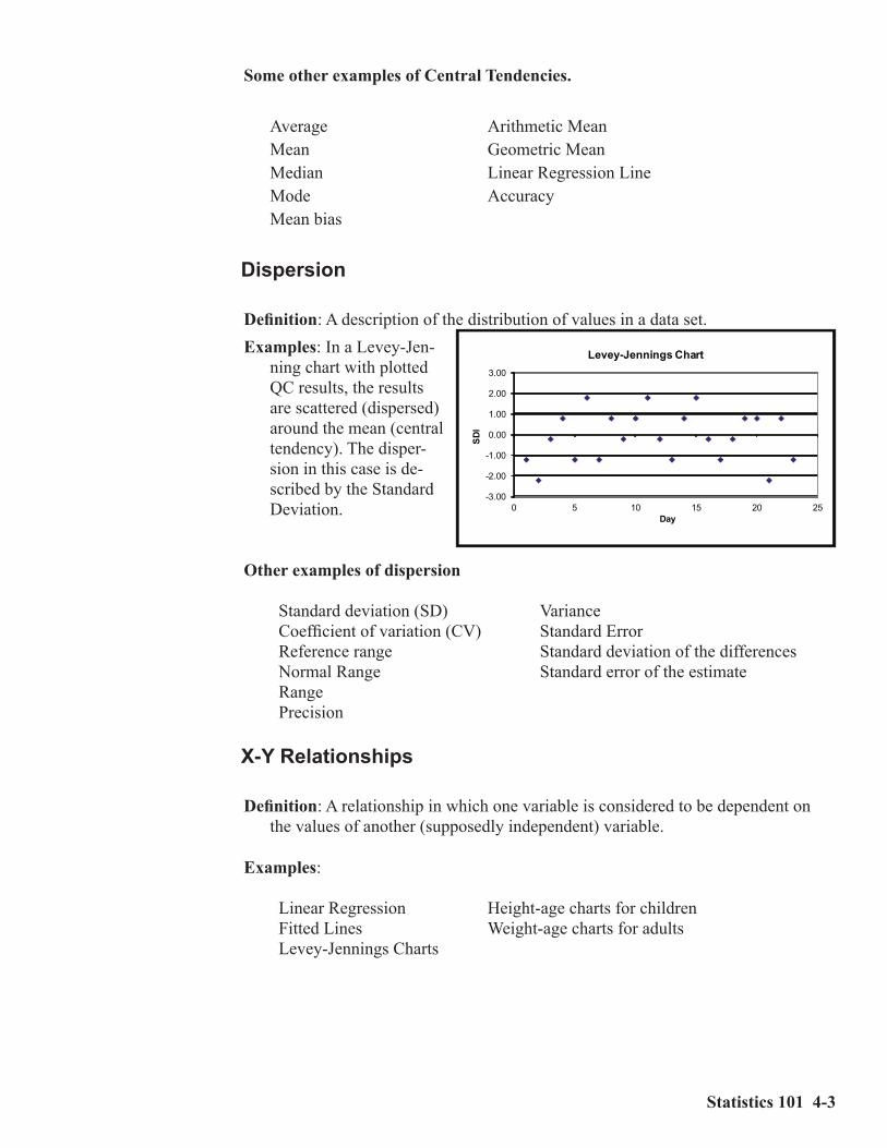
Dispersion
Definition: A description of the distribution of values in a data set.Examples: In a Levey-Jen-
ning chart with plotted QC results, the results are scattered (dispersed) around the mean (central tendency). The disper-sion in this case is de-scribed by the Standard Deviation.
Other examples of dispersion
Standard deviation (SD) Variance Coefficient of variation (CV) Standard Error Reference range Standard deviation of the differences Normal Range Standard error of the estimate Range Precision
X-Y Relationships
Definition: A relationship in which one variable is considered to be dependent on the values of another (supposedly independent) variable.
Examples: Linear Regression Height-age charts for children Fitted Lines Weight-age charts for adults Levey-Jennings Charts
-3.00
-2.00
-1.00
0.00
1.00
2.00
3.00
0 5 10 15 20 25
SDI
Day
Levey-Jennings Chart

4-4 Lab Statistics - Fun and Easy
At right is a graph of an X-Y relationship obtained when two instruments are compared for a certain analyte.
Measures of Central Tendency
One thing to keep in mind is that there are many different descriptors of the cen-tral tendency. Use of an inappropriate descriptor can be misleading particularly if the distribution is highly skewed.Mean: This statistic is calculated from the sum of all elements in the set and
divided by the number of elements. It is meaningful when the distribution of the numbers is not highly skewed. For example, the mean age of all the people present in a hos-pital nursery when the nurse is present is much higher than when only the infants are present. If only infants are present, the mean age is several days. Whenever the nurse is present, the mean age becomes years.
Average: See mean.Median: The median is the middle
of an ordered list of results. If the number of items (N) is odd, then it is the middle item. If N is even it is the average of the middle two items. In a skewed distribution, it better represents the central tendency than the mean. In the nursery example above, the median age would change little whether the nurse is present or not. In both cases, the median age would be a few days at most.
Linear regression line: One type of central tendency in an X-Y relationship. In this case, the line fitted through the pairs of results is the central tendency.
0
50
100
150
200
250
300
0 100 200 300
Y
X
Figure 4.1
Age (years)InfantsOnly
Infants &Nurse
Mean 0.02 1.3Median 0.02 0.02
Statistics 101 4-5
Measures of Dispersion
Since statistics only have real meaning when viewed in context, many techniques describe the distribution of the data and the regions of confidence we have in them.
Standard Deviation (SD) is the primary measure of the dispersion of a set of data. It is expressed in the same units as the mean. One problem with the concept of SD is that the sentence “Glucose has an SD of 10” is meaningless unless one knows the value of the mean.
Coefficient of Variation (%CV) is in fact a relative SD expressed in percentage units. Consequently, it is unitless. The fact that CV incorporates the value of the mean associated with the SD gives the term more meaning.
95% Confidence Interval describes the range within which a number would be expected to fall 95% of the time were the experiment to be repeated again. (Synonym: 95% confidence limits.)
Keep the food fat analogy in mind: If the Haagen-Daas ice cream container claims that its contents are 85% fat free, you can expect a 15% fat content (100%-85% = 15%). Similarly, with a 95% confidence limit, the number is expected to fall within that range 95% of the time. In other words, 19 times out of 20, the expectation will be correct. One time out of 20, it will be wrong.
2 SD Range: The 2 SD range, more accurately, is the interval from the mean - 2SD to mean + 2 SD. It has a 4SD width. It is another form of the 95% Confi-dence Interval. To be more precise, the 95% CI is a 1.96 SD range. Converse-ly, the 2 SD range is a 95.5% CI. For practical purposes, these two concepts are identical.
Standard Error of the Estimate describes the dispersion of data in the environ-ment of an X-Y relationship, namely the dispersion of data around a linear regression line.

4-6 Lab Statistics - Fun and Easy
Practical Applications
Table 4.1 illustrates several aspects of dispersion. The three sets of data all have means of 46. However their distributions are very different. The data in Set I has a range of 3 (from 45 to 48), the data in Set II a range of 15 (from 38 to 53) and the data in Set 3 a range of 25 (from 33 to 58).
Table 4.1Examples of Dispersion
Set 1 Set 2 Set345 43 4145 47 5347 52 3846 46 5845 38 3348 53 5645 42 43
Average 46.0 46.0 46.0SD 1.2 5.2 9.7%CV 2.5% 11.2% 21.0%Range 45 to 48 42 to 53 33 to 5895% CI 43.7 to 48.3 35.9 to 56.0 27.1 to 65.0Ratio (1) 1.11 1.56 2.40(1) The ratio is the upper 95% confidence limit divided by the lower 95% confi-dence limit.
Keep in mind that widening the dispersions of data means that the significance of individual results can change. All the numbers within the 95% CI are identical statistically. In the case of set 1, these statistically identical numbers range from 43.7 to 48.3. For set 3, they range from 27.1 to 65.0. The meaning of a value of 35 is very different when viewed from the perspective of the 95% CI of set 1 ver-sus that of set 3. When viewed from the perspective of set 1, it is a clear outlier. When viewed from the perspective of set 3, it is statistically identical to the other numbers in the set.
The most important thing to realize is that in the clinical laboratory environment, since all results within a 2 SD range of the mean are acceptable, all results in that range are statistically identical.
For some analytes, a 7% CV (e.g. hemoglobin) is unacceptable, while for other analytes (e.g. TSH), it may be excellent. That the 7% CV for hemoglobin is unac-ceptable because the CLIA ‘88 PT limits are 7%. As we will see later, you want a minimum of 4 CV’s inside the PT limits. Additionally at 14 g/dL, a 7% CV is 1.0 units which leads to a 95% CI of 12.0 to 16.0 units. This is 100% of the normal range. Consequently, this broad range significantly lowers the ability to distin-guish between health and disease for hemoglobin-related conditions.
Statistics 101 4-7
Outliers
Outliers are points obtained in a set of data which for some reason are considered to not be representative of that set. The usual reason for declaring a point an out-lier is because it represents an error.
Example: 45 results were obtained for a precision study from the XYZ analyzer. 44 of the results were in the range of 85 to 97. The 45th result was 81. Examina-tion of the sample cup for the 45th result showed it to be empty. The other sample cups had small amounts of specimen remaining in them. Since it can be shown that the suspected outlier was due to a short sample, it can be legitimately exclud-ed from the calculation.
Detection of Outliers
Determining whether points are outliers requires honesty and integrity. Otherwise the quality of the resulting statistics will be compromised. It is best to use criteria which require that outliers be VERY different from the remaining results.
A common example of inappropriate rejection of results thought to be outliers occurs with QC data. Some labs routinely exclude all values greater than 2 SDs from their calculation of their target SD’s for the next month. Consequently, their calculated SDs get smaller and smaller until in the limiting case, there is only 1 acceptable value left.
Remember that the purpose of statistical analysis is to predict future results. There must be good reason to define a point as an outlier. For example, the CLSI:EP5 Precision document defines outliers as those runs for which duplicate results are different by more than 5.5 times the SD calculated from the preliminary (within-run) precision data. Consequently, two results within a run have to be very differ-ent before the run can be rejected as outliers.
One issue is what criteria should be used to find outliers. A common (inappro-priate) practice is to declare all points that seem to be inconveniently located as outliers. What should be done is first to check to see if a typographical error occurred. If more than one outlier exists, then perhaps no outliers at all should be excluded as this indicates a potentially serious problem.
Distributions
Another way of looking at results is as a distribution. Typically distributions are viewed using a histogram such as the one in Figure 4.1. which shows the ages of the people including infants and nurses in a hospital nursery.

4-8 Lab Statistics - Fun and Easy
Statistical Terms used in Clinical Laboratories
Related to Method PerformanceAccuracy: The ability of a method to detect the correct amount of analyte when
assaying a specimen.Analyte Measurement Range (AMR) Verification: Verifies the AMR (i.e. the
reportable range). This experiment verifies that the method is accurate across the whole reportable range.
Recovery: The percentage of the correct value that a method detects. Recovery is closely related to accuracy. Most analytical claims are expressed in terms of recovery. 100% is the ideal recovery.
Calibration Verification: See Analyte Measurement Range Verification.Reportable Range: The range over which a method can report an accurate result
without diluting the specimen.Precision: The ability of a method to obtain the same answer on repeated assay
of the same specimen. Frequently analytical claims are expressed in terms of Coefficient of variation. Remember a method can be extremely precise and still be very wrong.The major different several types of precision are within-run, between-run, between-day and total. Within- run precision represents the precision in one group of specimens assayed together. Between-run represents the precision component of assays at several hours apart but within a day. Between-day represents the precision component over a period of days. Total represents all these elements. The two most important types of precision are: total and within-Run. Between-run and between-day are less important.
Sensitivity: The ability of a method to detect low concentrations of an analyte. Expressed in units of concentration. There are three types of sensitivity: Limits of Blank (lowest concentration detected which is significantly differ-ent from zero) (synonym: Analytical Sensitivity); Limits of Detection (lowest concentration for more none of the results will be zero) and Limits of Quan-titation (lowest concentration at which a result can be “reliably” measured, typically with a CV of 20 or 25%) (synonym: Functional Sensitivity).
Specificity: The ability of a method to accurately determine the concentration of an analyte in the presence of interfering substances. Commonly known as in-terference. Examples of interfering substances are those similar to the analyte (e.g. HCG interfering with the similar TSH) or those which interfere with the assay process (e.g. lipemia or hemoglobin interfering with spectrophotometric assays).
Relationship of Multiple MethodsMethod Comparability: Comparison of results obtained on analysis of a series
of specimens by two or more instruments or methods. The usual purpose to demonstrate the statistical identity of two laboratory methods. If two methods are statistically identical, one will be able to make the statement “These two methods are identical with 95% confidence”.
Statistics 101 4-9
Method Harmonization: Comparison of two or more production methods which measure the same analyte to demonstrate whether the results for the same specimen are statistically identical.
Related to Reference Intervals and Medical Decision PointsNormal Range: The range of concentrations of an analyte expected in a clini-
cally healthy population. This definition is the one required for verifying the reference range. The usual definition of this term is the central 95% of results found in this apparently healthy population. Those inclined toward great preci-sion in language call this the “reference interval of a clinically healthy popula-tion.”
Reference Range: The range of concentrations of analytes in a specimen which correspond to a specific clinical condition. One clinical condition is being healthy. In this case, reference range has the same meaning as normal range. Some other clinical conditions are disease conditions such as congestive heart failure or toxic drug overdose. Others include natural conditions such as pregnancy or strenuous exercise conditions. One common one for drugs is the therapeutic range.
Reference Interval: See reference range.Medical Decision Points (MDP): That concentration of analyte at which medical
decisions for appropriate treatment can change. Example: Cholesterol con-centration of 200 mg/dL. At concentrations below 200, no action is taken. At concentrations above 200, often drugs are administered to the patient to lower cholesterol.Obvious MDPs are often the lower and upper limits of the normal range. For glucose, there are several MDPs. The lower and upper limits of the normal range are two MDPs, typically about 70 and 110 mg/dL. A hypoglycemic MDP is about 25 to 50 mg/dL. A hyperglycemic MDP would be in the 250 to 800 range. Other MDPs include critical values or panic values.

4-10 Lab Statistics - Fun and Easy
Effects of Bad Lab Results 5-1
C h a p t e r
5Understanding Error and Performance Standards
In this ChapterCritical to good quality assurance is understanding experimental error. We dis-cuss:• Concepts and terms used to describe systematic, random and total error.• Concepts of allowable total error.• The basis for error budgets.• Error budgets including the 25% rule.• Different applications of 95% confidence limits.
Experimental Error
Definition: Error is the deviation of a single estimate of a quantity from its true value. (Carey and Garber - 1989)
Synonym: Uncertainty.
Life would be much simpler if every measurement on the same specimen gave the same result. However, reality is that repeated analysis of the same specimen often produces different results. This is due to the presence of error in the measuring process. This chapter will present a general discussion of what error is and how it can be managed in the clinical laboratory setting.
Some Error Is Expected
Error occurs because not all components of the measuring process are exactly the same for each measurement. Reasons for variations may include: • Instrument parts wearing out.

5-2 Lab Statistics - Fun and Easy
• Variations in reagent concentrations.• Contamination of the instrument. • Variations in calibrator concentrations. • Variations of concentrations within a single specimen over time.Consequently, some error is expected. At issue is not the elimination of error, but its management.
Managing Error
It is essential that the user understand important related concepts concerning the management of error. Some important elements are:• Understanding the concepts of error.• Defining specifications of allowable error.• Using statistical tools to measure error. • Error profiles for quantitative analytical methods.• The relationship of QC rules to allowable error concepts.• Motivating and supporting personnel so satisfactory results are produced.• Providing evidence to regulators that the work is satisfactory.
Concepts of Error
Four major types of experimental error are introduced and discussed: random er-ror, systematic error, total error and idiosyncratic error. Note that random, system-atic and total error can only be assessed after analysis of a number of samples.
Random Error (RE)
Definition: An error either positive or negative which cannot be predicted.Regulatory Requirement Addressed: Reproducibility or Precision.Experiment: Repeated analysis of the same specimen. The duration of some
experiments is only within a single run. Others are performed in one or more runs per day over a period of days
Statistical Terms Describing Random ErrorMean: An average of the results. This is the central tendency.Standard Deviation (SD): The dispersion of the results. Related terms include
within-run, between-run, between-day and total SDs.Relative Standard Deviation or Coefficient of Variation (CV): The dispersion
of results expressed as a percent of the mean.Standard Error of the Mean (SEM): The confidence interval of the mean; in
other words, the uncertainty in the true value of the mean.

Effects of Bad Lab Results 5-3
Statistical ToolsSimple Precision Module: Analyzes results obtained without regard to multiple
runs and/or days. This is the traditional precision analysis. Statistics obtained from this type experiment include: mean, SD and CV.
Complex Precision Module: Analyzes precision results obtained from an experi-ment which controls the following elements: number of replicates per run, number of runs per day with a minimum number of days. Calculations are done using an ANOVA analysis. Statistics obtained from this type experiment include: mean, within-run SD, between-run SD and total SD.
Systematic Error (SE)
Definition: An error that is always in one direction.
Linearity ExperimentRegulatory Requirements Addressed: Accuracy, reportable range, calibration
verification and linearity.Experiment: Analysis of specimens with defined analyte concentrations. The
following elements may be varied in this type of experiment: number of specimens, type of specimen, number of replicates, and range of specimen concentrations. Depending on these variables, the experiment can determine accuracy, reportable range and linearity, as well as verify calibration.
Method Comparison ExperimentRegulatory Requirements Addressed: Crossover experiment showing changes,
if any, in the medical decision point(s).Experiment: Analysis of specimens for which analyte concentrations are deter-
mined by two or more methods. Analyte concentrations are not defined in advance. Keep in mind that most crossover experiments only compare two existing methods. Only in rare instances do they show the relationship with truth.
Statistical Terms Describing Systematic ErrorSlope: The concentration dependent response of an analytical system.Proportional Error: The degree by which the slope differs from 1. Proportional
error is a component of SE.Intercept: The concentration independent response of an analytical system.Constant Error: The degree by which the intercept differs from zero. Constant
error is a component of SE.Bias: There are several definitions. The one applicable in this context is the
amount that the average Y value differs from the average X value.
5-4 Lab Statistics - Fun and Easy
Statistical ToolsLinearity and Calibration Verification: Analyze results from an experiment in
which the analyte concentrations of the specimens have defined relationships with respect to one another. Statistical results include slope, intercept, recov-ery and calibration verification. If analyte concentrations challenge the lower and upper limits of the reportable range, then the statistical results also include reportable range. If allowable errors are defined, results will include a decision as to whether the data set is linear within allowable error.
Assuming accurately prepared specimens, Linearity is the best statistical tool for measurement of systematic error.
Alternate and EP9 Method Comparison: Analyze results from two or more methods for the same analyte for specimens with undefined concentrations. Statistical results include slope, intercept, standard error of the estimate (SEE) and the bias at the medical decision point.
EP10: Analyzes 10 results a day from 3 specimens over a period of at least 5 days. Statistical results include linearity, precision, accuracy, carryover and drift. If the low and high specimens challenge the limits of the reportable range, this experiment will evaluate those limits as well. EP10 is an experi-ment designed to show whether a method is satisfactory or not. It does not have sufficient statistical power to determine sources of problems.
EP15: Analyzes two groups of specimens, one for accuracy and reportable range, the other for precision. This CLSI document is not explicitly implemented in EP Evaluator®. However, it is possible to perform this type of experiment by using the Linearity and Complex Precision modules.
Total Error (TE)
Definition: A combination of random and systematic analytical errors that esti-mates the magnitude of error that can be expected for a single measurement. (Carey and Garber - 1989).
The formula for a point estimate of total error is:TE = SE + (nSD * RE)
where RE is random error (i.e. 1 SD) and nSD (number of SD’s) ranges from 1.96 (95% confidence) to 4.5 (99.9997% confidence = Six Sigma). TE is evaluated at specific concentrations. It is especially important to evaluate TE at the medical decision points.
Effects of Bad Lab Results 5-5
Idiosyncratic Error (IE)
Definition: Error from non-methodological sources such as specimen mixups, dilution or transcription errors.
Since minimizing IE is an organizational and management issue for each facility, discussion of IE is outside the scope of this book.
Performance Standards (i.e. Total Allowable Error)
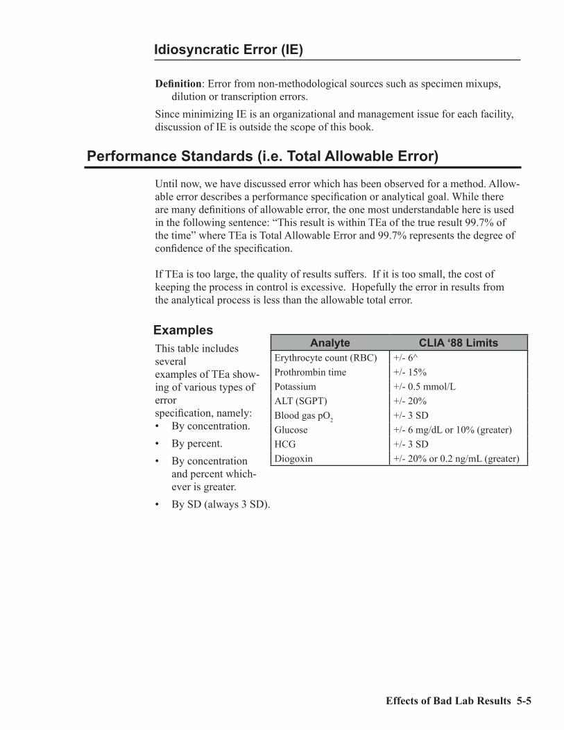
Until now, we have discussed error which has been observed for a method. Allow-able error describes a performance specification or analytical goal. While there are many definitions of allowable error, the one most understandable here is used in the following sentence: “This result is within TEa of the true result 99.7% of the time” where TEa is Total Allowable Error and 99.7% represents the degree of confidence of the specification.
If TEa is too large, the quality of results suffers. If it is too small, the cost of keeping the process in control is excessive. Hopefully the error in results from the analytical process is less than the allowable total error.
ExamplesThis table includes severalexamples of TEa show-ing of various types of errorspecification, namely:• By concentration.• By percent.• By concentration
and percent which-ever is greater.
• By SD (always 3 SD).
Analyte CLIA ‘88 LimitsErythrocyte count (RBC) +/- 6^Prothrombin time +/- 15%Potassium +/- 0.5 mmol/LALT (SGPT) +/- 20%Blood gas pO2 +/- 3 SDGlucose +/- 6 mg/dL or 10% (greater)HCG +/- 3 SDDiogoxin +/- 20% or 0.2 ng/mL (greater)

5-6 Lab Statistics - Fun and Easy
QC Failure
Often in the laboratory, QC failure is ignored. This occurs for many reasons, all of which at some level are excuses. These include:• Nothing bad will come of it (sometimes true).• It’s too hard to fix or we don’t have time to fix it.• The service person was just here and they didn’t know what to do.• Our QC isn’t out that much.• The only problem is with the external quality control.• We just repeated the QC specimen and it passed.
More important to our discussion here is the effect of QC failure. In fact, there are only two ways in which QC failure shows up externally:• Bad proficiency testing results.• Bad patient results
Regulatory Effect of QC Failure
The good news is that this type of QC failure becomes visible (in the US) no more than three times per year because that is how often proficiency testing is done. The bad news is that QC failure can exist for many months because proficiency testing (PT) does not happen very often. One fundamental reality of PT, however, is that labs get penalized if they fail. As a result, lab managers pay a lot of atten-tion to the PT process.
This figure shows graphically how QC failure occurs. Imagine what would happen if (in violation of the rules) you assayed the PT specimen 100 times. From all these results, you can calculate a mean and an SD. Then from those results, you can plot the results and get a curve similar to the one in this figure.
Two things can happen with respect to the analytical process: either systematic or random error or both can become excessive. These may cause QC failure to occur in the process. The important elements in this figure are:Target value represents the true result for this specimen. This corresponds to the
mean value returned for a proficiency testing specimen,Bias represents the systematic error. This corresponds to the difference between
your mean result and the target value.PT Limit represents TEa. This corresponds to the maximum allowable error
printed on the proficiency testing report for this specimen.

Effects of Bad Lab Results 5-7
Mean represents the average value for a PT specimen if you were to assay it many times.
Curve represents the distribution of results for that PT specimen if you were to assay it many times. An SD can be calculated from the results in that curve.
This figure has been set up so that the PT Limit is approximately 1 SD away from the mean. Statistically, about 17% of the results will be outside the PT limits. This number is shown by the hatched area to the right of the figure.
Let’s calculate how many results would be wrong if this scenario applied to all your tests. The typical hospital lab has a test menu of about 200 tests. If PT were performed on all those tests, 5 results per test or a total of 1000 results would be submitted to the PT provider (such as the CAP). Of those 1000 results, 17% or 170 results would be outside the PT limits. Not a happy thought. Most lab manag-ers get upset if there are more than 5 to 10 results (0.5 to 1%) which fail. In fact you want only a small fraction of 1% to fail.
Clinical Effect of QC Failure
Except for Proficiency Testing failures, labs usually are not overtly penalized for failure. In fact, often there is a reward in the form of additional testing (and revenue) as specimens are resubmitted to the lab to check the validity of previ-ous results. However there can be major systemic costs for bad patient results as shown in the following scenario:
Imagine a clinical protocol triggered by results exceeding a certain medical deci-sion point (MDP).
What happens if• 10% of the specimens with true results below the MDP in fact exceed it?• 10% of the specimens with true results above the MDP in fact do NOT exceed
it?In both cases, incorrect diagnoses may occur. These will result in extra cost and pain for both the health care system and the patient as the system deals with the consequences of poor lab results.

5-8 Lab Statistics - Fun and Easy
Error Profiles
An error profile describes the amount of random error expected over the reportable range (RR) of an analyte. It is expected that this error will vary with the concentra-tion of the analyte.
At the upper end of the RR, the SD tends to increase as the concentration of the spec-imen increases. At the lower end, the SD becomes more or less constant. The reason for this is that at the lower end, the SD approaches the noise level of the system and cannot go lower even with lower analyte concentrations.
The reason we are interested in the Error Profile is that it provides us with a mechanism of determining Total Allowable Error (TEa), otherwise known as Per-formance Standards.
The equation for the CV is shown below. The key point here is that while the CV rises rapidly at the low concentrations, it is relatively constant at higher concen-trations.
cv = 100 * SD / mean
The effect of these observations is to express the error for an analyte in terms of both SD (for low concentrations) and CV (for higher concentrations).
One case with real numbers is rep-resented by CAP survey results for bHCG for a major analyzer as shown in this table.
One important observations from this table are that all the CV’s are about the same (roughly 6 - 7%). While this is not always the case, one often observes that the CV’s at the upper 60 to 80% of the reportable range tend to be similar, namely within a range of 20% or so. CV’s in the lower range, untested in this survey, can be significantly higher.
HCG (Vitros ECi) (n=63)
Spec ID Mean SD CVC-11 26.97 1.65 6.1C-12 68.29 4.54 6.6C-13 90.61 6.39 7.1C-14 52.13 3.57 6.8C-15 82.47 4.84 5.9

Effects of Bad Lab Results 5-9
Also one should note the median value. In this example, the CV for specimen C-12 (6.6) is the median.
A graph showing more results for the same test (HCG) is also shown, this time from the New York State Proficiency Testing Survey. About two year’s worth of data are shown. The X axis is plotted on a log scale. Note that with a few exceptions, the CV’sat the upper end (above 30) are about the same. They are mostly clustered in the range of 5 to 7%. Similarly, the SD’s at the low end are clustered in the 1 to 2 units range. The median val-ues are shown in both cases.
This technique of using the median value from PT surveys is one of the key ap-proaches to establishing TEa. The process necessary to convert the median to TEa is discussed extensively in Chapter 6, Defining Performance Standards under the category of Total Achievable Error – based on Peer Group Surveys.
Error Budgets
As discussed above, TEa has two major components: allowable systematic error (SEa) and random error (RE). An error budget allocates a fraction of the total error for SEa and the remainder for RE as shown at right.
The next issue is what the appropriate division (i.e. budgeting) of these two error components should be.
• It is clear from the next figure that the worst case is allocation of all of the space in TEa to SAE. This is because no space at all is left for the inevitable random error. This virtu-ally guarantees Proficiency Testing failure (80% probability) for that test. The probability that any result will be more than TEa from its true value is about 45%.
Worst Case Minimum Case

5-10 Lab Statistics - Fun and Easy
• The minimum case (which is quite popular) is to set SAE at 50% and then to divide the remaining space into 2 SDs. The probability of failing PT on any given analyte is about 0.5%. However across a test menu of 100 analytes, if all had this same probability of failure, there would be a 50% chance (100 * 0.5%) that at least one would fail. The probability that any result will be more than TEa from its true value is about 5%.
• A more reliable case is the 25% rule. In this case, systematic al-lowable error is set to 25% of TEa. Then specify that 3 SDs be includ-ed in the remaining 75% random error space. The probability of failing PT with this model is about 0.03% (vs. the previous 0.5%). The probability that any result will be more than TEa from its true value is about 0.3%.
• The ideal case is Six Sigma. Here the amount of error is 3 parts per million (ppm). This contrasts with 45,000 ppm for the minimum case and about 3000 ppm for the 25% rule. Clearly a significant improvement if it can be achieved. The probability of failing PT is infinitesimal.
The formulas for the two types of error budget as used in this book are shown below.
Systematic error budget = 100 * SE/TERandom error space (RE space) = TE - SERandom error budget = 100 * RE space /(TE * nSD)
Establishing a Systematic Error Budget
In setting your systematic error budget (SEB), we recommend that it be between 25 and 50%. The ideal SEB is 25%. The reason that SEB not be less than 25% is that if it fails, then you are working to fix relatively small errors. The reason that the maximum value should not exceed 50%, is that then insufficient space is left for the random error component.
It is clearly a mistake to set SEB at 100%. While you will pass accuracy and linearity tests relatively easily, it completely neglects the very significant contribu-tion of random error to the probability of failing PT.
If the actual errors are within these specifications, the probability of failing PT be-comes exceedingly small. For details, see Chapter 11, Understanding Proficiency Testing.
In EP Evaluator®, SEB is used to calculate items such as the height of the linear-ity error bars and maximum bias for recovery purposes. These values are applied to statistical values such as the mean at each concentration. They are not applied to individual results.
25% Rule Six Sigma

Effects of Bad Lab Results 5-11
TEa = concentration * 10% = 200 * 0.10 = 20 mg/dL
SEa = TEa * systematic error budget = 20 * 25% = 20 * 0.25 = 5 mg/dL
Establishing a Random Error Budget
In setting your random error budget (REB), we recommend that it be in the range of 16 to 25%. While there may be some cases (i.e. for electrolytes such as sodium, chloride and calcium) in which it is difficult to get the REB to this level, we strongly encourage you to make the effort. The 25% value corresponds to the 25% rule. The 16% value corresponds to the Six Sigma effort. Furthermore if you set your SEB to 50%, then you must have your REB be no more than 25%, other-wise you have a relatively high risk of generating results which exceed the TEa.
Calculation of Allowable Systematic Error
Allowable Error calcula-tions start with the user entering the allowable total error (TEa). An example of TEa is the CLIA ‘88 PT limits for glucose of 10% or 6 mg/dL whichev-er is greater. When glucose concentrations are 60 mg/dL or less, TEa is 6 mg/dL, otherwise it is 10% of the glucose concentration. The second element is the systematic error budget (SEB). TEa and SEB are multiplied together to get an allowable systematic error (SEa). For the glucose example, if SEB is 25%, the SEa at 200 mg/dL will be 5 mg/dL.
Assessing Uncertainty
When a result is presented, there should be some indication of its quality. For example, a result of 10.0 ± 0.1 is very different from a result of 10 ± 3. In the first case, the range of possible results is 9.9 to 10.1, in the second, it is 7 to 13.
Confidence intervals are often used to show the range within which results are expected to occur. Confidence intervals typically are given for 95% (2 SD) or 99.7% (3 SD) limits. The 99.7% confidence interval will always be wider than the 95% interval.
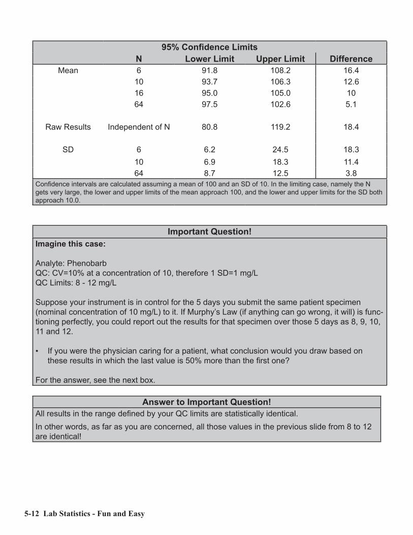
Examples of 95% confidence intervals for a set of data with a mean of 100, an SD of 10 with various numbers of results (N) are shown in the table below. Note how the confidence intervals decrease in size for the mean and SD as N gets larger. The confidence interval for the results themselves are independent of N. Note also that while N increases by a factor of 4, the confidence intervals only decrease by a factor of 2.
5-12 Lab Statistics - Fun and Easy
95% Confidence LimitsN Lower Limit Upper Limit Difference
Mean 6 91.8 108.2 16.410 93.7 106.3 12.616 95.0 105.0 1064 97.5 102.6 5.1
Raw Results Independent of N 80.8 119.2 18.4
SD 6 6.2 24.5 18.310 6.9 18.3 11.464 8.7 12.5 3.8
Confidence intervals are calculated assuming a mean of 100 and an SD of 10. In the limiting case, namely the N gets very large, the lower and upper limits of the mean approach 100, and the lower and upper limits for the SD both approach 10.0.
Important Question!Imagine this case:
Analyte: PhenobarbQC: CV=10% at a concentration of 10, therefore 1 SD=1 mg/LQC Limits: 8 - 12 mg/L
Suppose your instrument is in control for the 5 days you submit the same patient specimen (nominal concentration of 10 mg/L) to it. If Murphy’s Law (if anything can go wrong, it will) is func-tioning perfectly, you could report out the results for that specimen over those 5 days as 8, 9, 10, 11 and 12.
• If you were the physician caring for a patient, what conclusion would you draw based on these results in which the last value is 50% more than the first one?
For the answer, see the next box.
Answer to Important Question!All results in the range defined by your QC limits are statistically identical.In other words, as far as you are concerned, all those values in the previous slide from 8 to 12 are identical!

Defining Performance Standards 6-1
C h a p t e r
6Defining
Performance Standards
The concept of performance standards (PS) for the clinical laboratory is not new. This issue has been addressed in numerous conferences and papers spanning more than 40 years. Furthermore PS were established for about 75 common tests in the US by federal regulations in 1992 and then were finalized in 2003 (Federal Regis-ter - 2003).
Of the many reasons PS have not been widely adopted, there are two which are key: a) In many laboratories, there is no urgency to work according to PS; and b) PS are not available for most laboratory tests. It has been my observation that:• There is no consensus in our industry that we need PS except for the CLIA ’88
PT limits.• There is no consensus on how to establish PS.• There is no consensus on what those PS should be.
Achieving a consensus on these issues will likely take years. Fortunately, many are now working on this problem. I hope that this discussion will be an impetus so a consensus on these issues can eventually be established.
Our industry is heavily quantitative. However it does not universally accept the concept of quality goals. A common practice in the US is to set convenient preci-sion targets with the assumption that since these targets are “so tight”, no one will get hurt.
PS are used to define the two most important metrics for quantitative clinical labo-ratory tests: (1) allowable bias and (2) target SD values for routine quality control. These metrics define the quality of our results.

6-2 Lab Statistics - Fun and Easy
There are substantial benefits to defining performance standards for each test.• They can be used to set both target SD values for routine QC and allowable
bias. These two numbers define the quality of our primary product - patient results!! If either of these metrics is excessive, the ability to correctly interpret the results suffers. If either is too small, then the cost of keeping the test in control is excessive.
• A statement similar to the following (in this case for glucose) can be published for each test. “The results for this test are expected to be within 6 mg/dL or 10% of the true value 99.7% of the time.” I believe that the use of such statements would significantly help in the inter-pretation of laboratory results. It is my observation that only a small fraction of clinical laboratorians have a good sense of the quality of our product, clinical laboratory results. In fact, use of such statements could be a great marketing tool as labs would then be able to claim quality goals in their advertising.
Adding to the complexity of this problem is that there are many types of clinical laboratories, some of which are listed below. Clearly one single approach will not work in all cases.• Clinical laboratories operate in different regulatory environments. Conse-
quently, PS dictated by regulations from one jurisdiction will not apply to all.
• Specimens are obtained from multiple species. While the most common spe-cies of course is homo sapiens, there is an active community working with animals. As a consequence, species-specific criteria for establishing PS such as medical requirements, biological variation and reference intervals are not universally applicable.
• Clinical environments can be very different. A hospital clinical lab operates under very different rules than one in the pharmaceutical industry.
One fundamental problem is that PS definitions have never been systematically enumerated in one place. I will systematically list and evaluate each of the major definitions in turn.
Editorial Note:PS for clinical laboratory tests traditionally have been expressed as Total Al-lowable Error (TEa). I prefer the term “Performance Standards” because it is positive. It is easier for the uninitiated to understand than the formal term “Total Allowable Error” because the latter is technical and has negative con-notations.
Defining Performance Standards 6-3
Issues to be Addressed
On what basis should one define PS? Should there be a relationship to clinical metrics (i.e. medical requirements, biological variation, etc.) or should their val-ues be based on what is analytically achievable? In years past, I preferred clinical metrics. However I have found that this is not universally acceptable because as I will show below, there are many instances in which clinical metrics are unattain-able, unavailable or inappropriate.
The overall object should be to define PS for every test. These PS should be both attainable and defensible. Keep in mind also that there is almost always an ac-ceptable range for a PS, not just a single value.• Attainable means that the PS is analytically achievable by the process. • Defensible means that the PS has an acceptable relationship to the require-
ments of the clinical decision making process for that analyte. The analysis below applies to analytes for which quantitative results are reported. It does not apply to qualitative or semi-quantitative analytes nor to analytes mea-sured using amplification processes such as PCR.
Performance Standards Defined
Classes
There are three classes of definitions of PS: (1) clinical, (2) establishment and (3) deployment. Each has its role in understanding PS. Clinical defines the clinical or operational goals without specifying how the PS
metrics are calculated.Establishment definitions specify the algorithms which can be used to define PS.
The bulk of this chapter will relate to this class of definitions.Deployment definitions specify how PS metrics calculated in the Establishment
phase are converted into allowable bias as well as the target SD’s for routine quality control.
Clinical Definitions
Traditional Definition: “The amount of error that can be tolerated without invali-dating the medical usefulness of the analytical result ...” (Garber and Carey - 2010).
Biological Variation Definition: The amount of error derived from an experiment which estimates inter- and intra-individual biological variation (Fraser - 2001).
Regulatory Definition: The amount of error that can be tolerated without failing performance requirements established by a regulatory body.
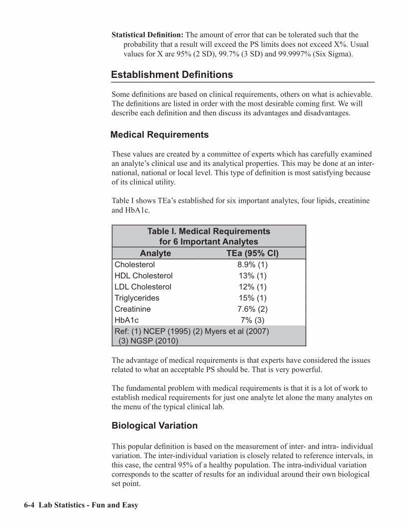
6-4 Lab Statistics - Fun and Easy
Statistical Definition: The amount of error that can be tolerated such that the probability that a result will exceed the PS limits does not exceed X%. Usual values for X are 95% (2 SD), 99.7% (3 SD) and 99.9997% (Six Sigma).
Establishment Definitions
Some definitions are based on clinical requirements, others on what is achievable. The definitions are listed in order with the most desirable coming first. We will describe each definition and then discuss its advantages and disadvantages.
Medical Requirements
These values are created by a committee of experts which has carefully examined an analyte’s clinical use and its analytical properties. This may be done at an inter-national, national or local level. This type of definition is most satisfying because of its clinical utility.
Table I shows TEa’s established for six important analytes, four lipids, creatinine and HbA1c.
Table I. Medical Requirements for 6 Important Analytes
Analyte TEa (95% CI)Cholesterol 8.9% (1)HDL Cholesterol 13% (1)LDL Cholesterol 12% (1)Triglycerides 15% (1)Creatinine 7.6% (2)HbA1c 7% (3)Ref: (1) NCEP (1995) (2) Myers et al (2007)(3) NGSP (2010)
The advantage of medical requirements is that experts have considered the issues related to what an acceptable PS should be. That is very powerful.
The fundamental problem with medical requirements is that it is a lot of work to establish medical requirements for just one analyte let alone the many analytes on the menu of the typical clinical lab.
Biological Variation
This popular definition is based on the measurement of inter- and intra- individual variation. The inter-individual variation is closely related to reference intervals, in this case, the central 95% of a healthy population. The intra-individual variation corresponds to the scatter of results for an individual around their own biological set point.

Defining Performance Standards 6-5
Two compilations of biological variation (BV) values are available, one for about 270 analytes (Ricos et al - 2004) and one for 42 analytes (Lacher - 2005). Some BV are extremely tight (i.e. sodium and calcium) while others are very relaxed (i.e. ALT). Table II shows TEa’s derived from BV for several analytes.
Table II. Biological Variation - Desirable Performance Standards
Analyte Ricos et al Lacher et alALT 32.1 33.4Albumin 3.9 4.6Total Bilirubin 31.1 32.0Calcium 2.4 4.2Cholesterol 9.0 12.7Glucose 6.9 10.6Sodium 0.9 1.6
While this approach is attractive because PS are defined by metrics which have some clinical relevance, the fundamental issues are what that clinical relevance is and then how to apply it. Fraser (2001) has shown that the clinical relevance is that given successive results for the same test on the same patient, one can estimate the probability that those results are different based on intra-individual variation. While this metric may seem to some to be valuable, a number of ques-tions both practical and theoretical can be raised which indicate that it may not be as valuable as one might initially believe.
Another major difficulty is that in a number of cases PS as determined from bio-logical variation is so tight that it is unattainable. For example, the PS for sodium is 0.9%. For many instruments, one process SD is 0.65%. Consequently, that PS is unattainable as it is less than 50% of what is achievable (about 2.7%).
In spite of these difficulties, PS as determined from biological variation remains a popular approach, particularly in certain European labs.
Reference Interval - Tonk’s Rule
This very simple approach was proposed (Tonks - 1963) as a metric for what con-stitutes an acceptable result for proficiency testing. TEa is 25% of the reference interval, expressed as a percent or 10% whichever is less.
TEa = 25% * RI.100 or 10%, whichever is less
where RI.100 = 100 * (RI range)/(mean of RI limits)
This approach seems to be very nice because it is clinically related, namely to the magnitude of the reference interval (RI). Its problem is that it works with very few tests. In many cases, TEa is not achievable especially when the lower limit of RI is near zero.

6-6 Lab Statistics - Fun and Easy
Regulatory Requirements (CLIA ’88 or EQAS)
Those regulating clinical laboratory performance in the United States and else-where have established maximum performance standards for many important analytes (Federal Register - 2003). For this, our industry should be grateful as this was the first list of PS for a significant number of analytes. Values for selected analytes are shown in Table III.
Table III. Selected PT Values from CLIA ‘88Analyte CLIA ‘88 Limits
Erythrocyte count (RBC) +/- 6%Prothrombin Time +/- 15%Calcium +/- 1.0 mg/dLALT (SGPT) +/- 20%Blood gas pO2 +/- 3 SDGlucose +/- 6 mg/dL or 10% (greater)HCG +/- 3 SDDigoxin +/- 20% or 0.2 ng/mL (greater)
The complete list of quantitative analytes is shown in Appendix A. When the regulatory requirement is expressed as target +/- 3 SD, it refers directly to the next approach “Total Achievable Error - based on Peer Group Surveys.”
There are two advantages of this PS determined using the CLIA ‘88 PT Limits:• By definition, the values are acceptable to the regulators.• With some exceptions, the values seem to be clinically responsible.
There are a number of disadvantages to these values apart from their clinical util-ity:• Values have been established for only 75 analytes.• There are many labs (i.e. outside the US) which are not required to use these
values.
It must be pointed out that other organizations and jurisdictions have established regulatory requirements for clinical labs including Australasia and Saskatchewan. These values are available on our website (www.datainnovations.com).
Total Achievable Error – Based on Peer Group Surveys
Unlike several approaches described above, this one is based on the analytical performance of which a process is capable. Peer Group Survey results may be easily obtained from PT providers such as the CAP for a large number of analytes. This approach is derived from the CLIA ’88 specification of “target +/- 3SD.”

Defining Performance Standards 6-7
This rule attempts to define for the general case, what is meant by 3 SD. In the case of the PT surveys, it is applied only to individual specimens. A simplifying approach is needed so PS can be easily defined for use across the whole reportable range.
An simple approach is related to the CLIA ‘88 PT specifications for PS as a concentration or a percent or both. The problem then is how to derive appropriate numbers. In some cases, one only needs to establish a concentration or a percent, whereas in others, one needs to establish both.
The core calculation of this approach is to calculate the median CV for enough specimens and then to multiply it by three. The CV is one form of SD. This ap-proach provides a reasonable approximation of the achievable error.
Enough specimens is defined as a minimum of 6. It is important to get results from multiple survey cycles. The minimum is six (two specimens per cycle) or ten (five specimens per cycle). Ideal is 15 to 20 specimens.
Our approach divides the reportable range into two general regions, an upper region which typically is the upper 50 - 80% of the reportable range and a lower region which is everything else. Basically one can use an error profile approach to calculate a median CV in the upper region and a median SD near the low end of the reportable range. Once you have determined an appropriate median SD or CV, then multiply it by 3 to calculate the PS.
The key issue that you need to keep in mind when using this approach is that the median fairly represents the error of your method in the applicable range. Several things to check:• Are there enough specimens in the sample from which you calculate the me-
dian?• Are there enough specimens (at least 4) in the applicable range?• Are there enough labs (at least 10) participating in the survey?
The advantage of this approach is that PT or EQAS results are readily available for more analytes. Furthermore, the calculated PS is attainable which is a major advantage.
There are a couple of disadvantages of this approach:• Various instruments have different median CV’s. Sometimes, the differences
across all the instrument groups can be as much as a factor of 2 or more. If your instrument is one of those with the higher CV, then you may want to con-sider carefully whether that relatively high PS is satisfactory in your environ-ment. A second alternative is to switch to a different method if the magnitude of the errors of the existing method are unacceptable.
• Insufficient data. If a test is not established, this approach utterly fails simply because there are no peer group data.

6-8 Lab Statistics - Fun and Easy
Total Achievable Error – CLSI:EP21
This approach defines TEa from a laboratory experiment which resembles EP9 Method Comparison. (ref. CLSI:EP21)
The advantage of this approach is that it is based on what is experimentally achievable and is not dependent on the analytical performance of other labs.
Its disadvantage is that it is a lot of work to do.
Total Achievable Error – Responsible Precision Estimate (RPE)
In this approach, PS are established using the long-term precision performance of the method. These data among other things, define the smallest PS which is consistently achievable for the method (minimum TEa). In other cases, one can establish a more realistic TEa.
Potential sources of an RPE include: • Medians of the CV’s of peer group QC results. It is preferable if the data on
which such an estimate is based comes from multiple labs over a period of many months. One may use results across multiple lots of QC materials pro-vided the concentrations are in the appropriate region of the reportable range. Similarly, one may use results from multiple brands of instruments provided the precision profiles for those instruments are similar.
• Total precision estimates from the vendor’s package insert for a process. The values used should be the vendor’s published estimate of total precision per-formed using an EP5 experiment (CLSI:EP5). The results should be calculated from one or more specimens in the range for which the TEa is being calcu-lated.
• One’s own monthly QC data. Data from this source should only be used when other precision estimates are not available such as for home-brew methods.
• Calculation processAggressive RPE TEa = 3 * RPEAchievable RPE TEa = 4 * RPE
An advantage of this statistic is that it has the potential of establishing a PS that is attainable.
The greatest danger with this approach is the potential that it is biased by results from poor QC practices. This would make the RPE much larger than it should be.
Defining Performance Standards 6-9
Deployment Definitions
Biological Variation
The algorithm used to calculate TEa uses values already calculated for the target CV and allowable bias. Fixed formula25% Rule allots 25% of TEa to systematic error. In addition, the target SD is 25%
of the TEa. There is nothing special about this rule except that it is a very easy way to allocate the total allowable error space to both random and system-atic error. One should also remember that there are cases in which it doesn’t work. An advantage of this rule is that about 3000 results out of a million will exceed TEa.
Traditional practice often allocates 50% of TEa to systematic error. The target SD is 25% of the TEa. With this approach, about 23,000 results per million will exceed TEa.
Six Sigma is similar to the 25% rule in that it also allots 25% of TEa to system-atic error. However, the target SD is 16% of TEa. With this approach, only 3 results out of a million will exceed TEa.
Relative Allocation
Allocation is based on the relative magnitudes of systematic and random error to total allowable error coupled with flexible assignation of QC rules. Refs: West-gard (2001) and Brooks (2002).
6-10 Lab Statistics - Fun and Easy
Defining PS for Established Methods
The following logic should be used to define TEa’s for established methods. These methods are those for which frequent surveys are performed, such as those circulated by the CAP, some other PT provider or an EQAS provider. This is not for “home brew” tests not performed by a limited number of laboratories. Perform the steps in the order below:• If medical requirements have been established for the analyte and are appli-
cable, use them!!• Consider values specified by regulatory bodies and those from Peer Group
Surveys. If one is significantly smaller than the other, use it.• If the value selected is derived from a Peer Group Survey, round it up or down
gently.Keep in mind that the point of the process is to define a PS which is attainable and defensible. In most cases, there is a range of possible PS’s which can be cho-sen. Use your clinical judgement to decide which value to select.
Near the end of this chapter, there are a number of worked out examples. This ap-proach has been implemented in EP Evaluator®, Release 10.
Comprehensive Approach for Defining PS
This approach can be used for methods which are: a) not widely used; b) are not present in the menu of tests from the PT or EQAS providers; or c) use of the “Es-tablished Test” approach is unsatisfactory. Keep in mind that in most cases, data from a limited number of these sources will be available.
• If clinical requirements are available, use them. If you have adequate resourc-es especially interested experts, consider establishing your own.
• If a reference interval has been established, consider Tonk’s Rule. If the refer-ence interval is near the low end of the reportable range, its usefulness will not be likely.
• Consider biological variation data if they exist. In a number of cases, such values are not achievable. However they may give you a starting point.
• Regulatory limits not necessarily from your jurisdiction.• Calculate from peer group survey results.• CLSI:EP21. Implementation of this will require the performance of a carefully
designed experiment in which results are entered for two methods, the pro-posed method and one which someone else has established.
• Responsible Precision Estimate data will almost always be available. Some of the values obtained from these sources may be so tight that they are not achievable. Others are so wide that they are indefensible. We recommend that you define minimum and maximum values for PS. The minimum value is the best your equipment can reasonably achieve (i.e. the Aggressive RPE described above). The maximum value is the regulatory limit or the Maximum TEa as de-scribed below whichever is less.

Defining Performance Standards 6-11
Low End Performance Standards
In many cases, the concentrations of the linearity specimens at the low end of the reportable range are such that the PS calculated for the upper portion of the reportable range fails. For example, suppose the defined concentration of a low end specimen is 5 for ALT (TEa=20%, typical reportable range is about 0 to 1000 U/L). The measured result is 7. In most cases, such values are good enough from a clinical perspective. The problem is that in this case, it fails accuracy because 7 is outside the acceptable range of 4 to 6 (5 +/- 20%).
The purpose is to define a concentration term for TEa. There are two ways to do it:• Multiply an SD at a concentration near the low end of the reportable range by
3. (Recommended).• Define a clinically insignificant concentration which works. The key is that the
concentration really be clinically insignificant.
Limits defined by Performance Standards
My personal feeling is that PS should rarely exceed 30%. The only exceptions that I can think of are for those analytes such as viral loads which are measured by amplification assays (i.e. PCR).
PS define upper limits for two major performance metrics. They are:• Upper limit for bias is 50% of PS.• Upper limit for a target SD is 25% of PS.One major implication of this rule is that the maximum %CV for any test should not exceed 7.5% (25% of the maximum allowable TEa of 30%).
Defining Performance Standards - Case Studies
Several examples of the process you can use to establish performance standards are shown below. There are a number of formulas involved in calculating these numbers.
Summary of Defining Performance Standards for Established Methods
Clinical Requirements Use as isRegulatory Requirements Use as isPeer Group Survey Factor*Median CV. Factor is usually 3 (default), can be
2 or 2.5 if specified by the regulators.Low end SD 3 * low end SD or value which is clinically insignificant.
The following examples are meant to illustrate the process. The numbers calcu-lated may not be applicable to your environment.

6-12 Lab Statistics - Fun and Easy
Case Study: Sodium
Starting ParametersUnits mmol/LMedical Requirements NoneRegulatory Requirements 4 units 4/140 = 2.85%Peer Group Survey Median CV
1.23% 3 * PGS = 3.7%
Low end SD n/a The instrument in this case is the fictitious Eximer 250. PGS data is from New York State PT Surveys.
Calculation Process:Medical Requirements: None• Regulatory Requirements: 2.85%• PGS Value: 3.7% -- too large (exceeds maximum of 2.85%)
Sodium is one of those tests for which its QC needs to be monitored very closely. I know of one lab which assays sodium in duplicate and then reports the mean in order to improve the precision. I recommend using the tightest feasible values which in this case corresponds to the regulatory requirements.
You have two major options: • Use TEa as defined by the regulatory requirement.• Lower the SD even more by devising a procedure to improve the precision
such as assaying each specimen in duplicate and then averaging the two re-sults.
Case Study: HDL Cholesterol
Starting ParametersUnits mg/dLMedical Requirements 13%Regulatory Requirements 30%Peer Group Survey Median CV 5.4% 16.2%
The PGS results are from the New York State PT Surveys for the Siemens Dimen-sion RXL.

Defining Performance Standards 6-13
Calculation Process:Medical Requirements: 13%PGS value: 16.2%Options:• Medical Requirements: 13%• Regulatory Requirements: 30%• PGS Survey: 16.2%
In this case, Medical Requirements have been specified. This then sets an upper limit for TEa of 13% which trumps the Regulatory Requirement of 30%.
Case Study: pO2
Starting ParametersUnits mm HgMedical Requirements NoneRegulatory Requirements 3 SDPeer Group Survey Median CV 3.9% 3 * 3.9 = 11.7%
The PGS results are from the New York State PT Surveys for the Siemens 845 instrument.
Calculation Process:• Medical Requirements: None• Regulatory requirements specify 3 SD. This translates to forcing the use of 3 *
PGS value.• PGS value: 11.7%
Options:• Regulatory Requirements (also PGS value): 11.7% rounded up to 12%.• TEa for pO2 could be set in the range of 8 to 12 mmHg.

6-14 Lab Statistics - Fun and Easy
Case Study: Free T4 (Comprehensive Approach)
Starting ParametersUnits pMol/LReportable Range (AMR) 3.9 to 77.2Reference Interval 10.3 to 24.5Medical Requirements NoneBiological Variation - TEa 9.9%Peer Group Survey Median CV
7.1% 3 * 7.1% = 21.3%
Regulatory Requirements NoneResponsible Precision Esti-mate
6%
I initially did this calculation during a trip to the Netherlands in 2005. The instru-ment was the DPC Immulite 2500. Much of the data was taken from the package insert for this instrument. The Peer Group Survey data was taken from the SKML (Dutch Clinical Chemistry Society) survey results. The Nether-lands at that time, had no regulatory requirements for any clinical laboratory tests. In the US, the CLIA requirements are +/- 3SD.
Calculation Process:• Minimum TEa (3 * RPE): 18% (while possible, difficult over long-term)• Maximum TEa: 30% (from Rhoads’ maximum TEa rule)• Medical Requirements: none• Biological Variation: 9.9% (unachievable)• PGS value: 21.3% - round to 20 or 25%• Achievable TEa from 4*RPE: 24%
Options:• Defensible range: 18 to 25%• Achievable range: 20 to 25%

Managing Quality Control 7-1
C h a p t e r
7Managing Quality Control
In This Chapter
Quality control is an important element in maintaining the quality of laboratory results. Unlike the other elements, it is used on a daily basis. QC is placed in the context of total allowable error (TEa) (i.e. Performance Standards). We discuss:• Concepts in quality control • Definition of key terms • Definition of QC rules• Tips on managing QC• In the event of QC Failure
CLIA ‘88 requires that for each instrument and analyte for which results are reported, at least two levels of QC are to be tested. This requirement is good laboratory practice because it requires the operator to demonstrate on every day of operation that the analytical system is working correctly.
Establishment of QC target val-ues is an important task because if well done, it allows the labo-ratory to set valid limits with a minimum of confusion. Also the laboratory’s results will be more consistent.
In a Levey-Jennings chart, the target mean is the central tenden-cy which is the expected result. The target SD (along with some QC rules) describes the magnitude of the region around the target mean within which the results will be acceptable.
The chart above shows an example of a well-behaved case. In this case, about 95% of the results are scattered in the 2 SD region above and below the mean.
-3.00
-2.00
-1.00
0.00
1.00
2.00
3.00
0 5 10 15 20 25
SDI
Day
Levey-Jennings Chart - Good Month
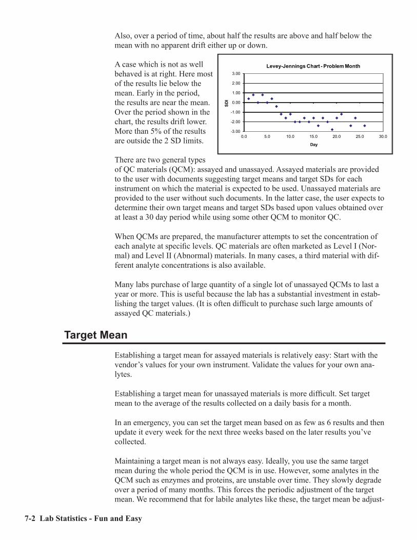
7-2 Lab Statistics - Fun and Easy
Also, over a period of time, about half the results are above and half below the mean with no apparent drift either up or down.
A case which is not as well behaved is at right. Here most of the results lie below the mean. Early in the period, the results are near the mean. Over the period shown in the chart, the results drift lower. More than 5% of the results are outside the 2 SD limits. There are two general types of QC materials (QCM): assayed and unassayed. Assayed materials are provided to the user with documents suggesting target means and target SDs for each instrument on which the material is expected to be used. Unassayed materials are provided to the user without such documents. In the latter case, the user expects to determine their own target means and target SDs based upon values obtained over at least a 30 day period while using some other QCM to monitor QC.
When QCMs are prepared, the manufacturer attempts to set the concentration of each analyte at specific levels. QC materials are often marketed as Level I (Nor-mal) and Level II (Abnormal) materials. In many cases, a third material with dif-ferent analyte concentrations is also available.
Many labs purchase of large quantity of a single lot of unassayed QCMs to last a year or more. This is useful because the lab has a substantial investment in estab-lishing the target values. (It is often difficult to purchase such large amounts of assayed QC materials.)
Target Mean
Establishing a target mean for assayed materials is relatively easy: Start with the vendor’s values for your own instrument. Validate the values for your own ana-lytes.
Establishing a target mean for unassayed materials is more difficult. Set target mean to the average of the results collected on a daily basis for a month.
In an emergency, you can set the target mean based on as few as 6 results and then update it every week for the next three weeks based on the later results you’ve collected.
Maintaining a target mean is not always easy. Ideally, you use the same target mean during the whole period the QCM is in use. However, some analytes in the QCM such as enzymes and proteins, are unstable over time. They slowly degrade over a period of many months. This forces the periodic adjustment of the target mean. We recommend that for labile analytes like these, the target mean be adjust-
-3.00
-2.00
-1.00
0.00
1.00
2.00
3.00
0.0 5.0 10.0 15.0 20.0 25.0 30.0
SDI
Day
Levey-Jennings Chart - Problem Month

Managing Quality Control 7-3
ed monthly based on a long term moving average such as a 3 month moving aver-age. For stable analytes such as electrolytes and glucose, the target mean should be adjusted only if justified by factors such as changes in calibrators.
One way changes in means are validated is to compare one’s own target values with those for other laboratories (peer group comparison) for the same analytes and instruments. One’s values should be similar to those of the other laboratories.
Target SD
There are two general approaches to establishing the target SD.
1 Base it on the SD calculated from the set of results used to calculate the target mean. This is the traditional approach.
2 Establish a value for the target SD which is somewhat larger than the SD cal-culated from the routine QC results and use it over a long period of time.
Once the target SD is established, in most cases, you can continue using it or a close equivalent even across lots of QCM as long as the mean values are similar. In other words, you can use an SD after adjustment on successive lots of Level 1 control. To use it across lots of QCM, calculate the CV from the SD of the senior lot, then for the junior lot, calculate the SD from that CV.
Given identical QC rules, the one with the larger target SD will have fewer in-stances of QC failure. Therefore it is in the laboratory’s economic best interest to use the larger target SD. If there is no significant downside in accepting a larger error, then use the larger value. If the target SD is significantly larger than the observed SD, a different set of QC rules should be considered for use.
To use the first option, calculate the mean and SD from the QC results obtained over as many months as possible (at a minimum, the previous month). Avoid as much as possible basing the target SD solely on just the previous month’s calcu-lated SD because it is too unstable to be reliable.
To use the second option, set target SD’s based on a combination of what is need-ed and what is possible for that method. If what is possible does not meet minimal Performance Standard requirements, then that method is unsatisfactory.
A target SD based on PS should be in the range of 16 (Six sigma) to 25% (25% rule) of the PS.
The next issue is how to calculate the value of the target SD based on the 25% Rule. For the 75 analytes for which CLIA has set proficiency testing (PT) limits, TEa can be considered to be the PT limit at the target mean.
For the enzyme ALT, for example, the PT limits are 20% of the target mean. If the target mean is 100 IU/L, the PT limits are 25 IU/L (25% times 100 IU/L). The target SD is then set to 25% of the PT limits or 6.3 IU/L. For many instruments, the observed process SD is about 3 or 4 IU/L. Since this is significantly smaller

7-4 Lab Statistics - Fun and Easy
than the target SD, it will be easier to operate this process since there will not be as many QC failures. Also in this case, use a QC rule such as 1-2S, certainly not 2-2S.
For sodium, the PT limits are 4 mMol/L. The ideal target SD would be 1.0 mMol/L. Since on many instruments, a value this small is hard to achieve, one may have to accept a value somewhat larger.
QC Rules
There is a long, rich and complex history to QC rules. Numerous scientific papers have been written over the last quarter century describing and analyzing many rules. The most common are known as the Westgard rules, named after James O. Westgard, Ph.D. (Westgard Website) who popularized them.
Westgard and others have defined a series of rules designed to detect when an ana-lytical system is no longer producing results which are in total control. An ideal rule would immediately detect every instance in which a system deviates from correct operation (no false negatives). Furthermore, it would produce NO false alarms (no false positives). However, there are no ideal rules. All rules ignore er-rors which are not totally egregious (at least for a while) and identify other events as QC failure even though they do not correspond to problems.
Several of the more common rules are listed below.
1-2S: If one result is more than two SDs away from the mean, QC failure is de-clared. This rule, popular in many laboratories, detects a great many problems. However, it also generates a large number of false alarms. If the SD value is calculated from the routine QC results, one would expect 5% of the values to be outside the limits. If this rule is implemented for 20 tests on an instrument, the target SDs are set to the observed SDs and the process is in control, at least one QC failure can be expected about 65% of the time. This rule is widely (and mistakenly) used in clinical laboratories.
2-2S: If two consecutive results either in the same or different QC materials are more than two SDs away from the mean, QC failure is declared. This rule is recommended in the CLSI document on internal quality control. It is much less sensitive to false alarms. This rule is recommended for most analytes.
1-3S, 1-3.5S: If one result is more than 3 or 3.5 SDs away from the mean, QC failure is declared. The purpose of this rule is to detect gross analytical prob-lems. False alarms from this rule will be relatively rare. The downside is that it will not detect developing problems at an early stage.
It turns out that not only is selection of the appropriate rules important, but that the frequency at which the QC samples are run is also important.

Managing Quality Control 7-5
Tips on Managing QC
We strongly recommend periodic reality checks (at least once every 2 months) in which you compare your means and SDs with those of other labs using the same instrument and analytes. This can be done using the results interlaboratory comparisons of QCMs and CAP surveys. Another reality test is to use Average of Normals (see next section in this chapter).
Calculate, review and file the actual means and SDs from all your QC results every month. In a system operating properly, you will not see large changes in the values. This is an important reality check. The results from each instrument will be slightly different from the next. One of your goals should be to make sure that the differences are not significant.
In the Event of QC Failure
What should a lab do if their QC fails?
One practice in many labs is that after a failure, the QC specimens are assayed repeatedly until it passes. This practice is inappropriate because it will not assure good results. For example, suppose this QC failure occurred because of a 2 SD shift in the mean with the underlying reason being that the reagents had deteriorat-ed. In this case, you would detect the failure fairly soon. However if you repeated it several times, inevitably some of the QC results would pass and then accord-ing to this practice, you would not have to determine the source of the problem. Consequently, the underlying cause of the failure would continue and the quality of patient results would be compromised.
To properly deal with the issue of QC failure, CLSI in their document on Quality Control (CLSI:C24) says it well:
“Appropriate response to an out-of-control situation is to troubleshoot the procedure, take appropriate corrective action, and then confirm successful correction by assaying QC materials. If the problem has been resolved, then results for all patients that have been assayed or reported since the last suc-cessful QC event must be evaluated for significance of the error condition on the clinical suitability of the results. Measurements for significantly affected patient results must be repeated, using properly stored samples, and corrected reports issued.” (quoted with permission)
The point of all this is to ensure patient safety. If the correctness of any results is uncertain, then immediate steps must be taken to ensure that correct results are available as soon as possible to the caregiver.

7-6 Lab Statistics - Fun and Easy
Average of Normals
Average of Normals (AON) compares median values from all the patient results from a given period with the medians of previous periods. A signifi-cant change in the median val-ue indicates that there has been a change in systematic error. This figure shows an example in which one shift occurred on May 9 and a more lasting shift started on May 16. There are several issues to understand with respect to this approach:• It makes the assumption that the mix of patients in the tested population is
relatively constant. Consequently if there is a change in the population, the ability of this approach to detect problems is compromised. This can happen in two major situations:• The patient mix on weekends is often significantly different from that on
weekdays because the workload is frequently much smaller, to say nothing about the mix of patients.
• The fact that certain clinics are held on particular days of the week can in-troduce false positives. A diabetic clinic, for example, would have a larger than usual of patients with high glucose related results. This could cause a significantly different patient mix.
• AON works best when the number of specimens (N) is large. With smaller N’s, the problems will still be detected, but it will take longer.
• AON works best when the ratio of the SD of the process is relatively large compared with the SD of the specimen population. In the best cases (analytes like sodium and calcium), problems can be detected with less than 100 speci-mens. In other cases such as triglyceride and cholesterol, it can take 1000 specimens or more to detect such problems.

Performance Validation Experiments 8-1
C h a p t e r
8Performance Validation
Experiments
In This Chapter
Most CLIA ‘88 requirements are established or verified experimentally. We dis-cuss:• The types of experiments which may be used to establish or verify each CLIA
technical requirement.• Guidelines for testing new instruments.
CLIA ‘88 technical regulations and good laboratory practices require that each laboratory should check from 3 to 7 statistical parameters for each new quantita-tive method adopted before patient results are reported.
Some individuals may believe that all these items have already been checked for each instrument by the vendor before they applied for FDA clearance. Just because a vendor has received clearance to market an instrument, does not mean that the instrument in your lab always reports correct results for all its analytes. In fact, most instrument vendors check out the operations of each instrument while it is being installed in your lab.
Question: You have just received a tool which you use to provide information to your clients. How important is it to you that the information is correct?
Question: If the instrument provides wrong answers, who do you want to know about it first?
Many of us know of occasions when a friendly physician will call the labora-tory and ask if a certain test is running high (or low). However the kindness of that physician does not excuse poor QC/QA practices.

8-2 Lab Statistics - Fun and Easy
Startup Requirements
The following parameters are a practical, systematic check of instrument per-formance. The experiments to evaluate each parameter are listed below. To the degree possible, references will be provided to the chapter which describes the experiment in detail and also to the relevant statistical module in EP Evaluator®.
Accuracy: A CLIA ‘88 requirement. Accuracy is the ability to measure the cor-rect amount of analyte present in the specimen. Evaluate this parameter using a linearity style experiment. In EP Evaluator®, the Linearity module assesses accuracy. See Chapter 10, Interpreting Linearity Experiments for discussion of this issue.
Linearity: A CAP requirement for some laboratory disciplines. There are several definitions of linearity, all of which show that a result does not differ from a straight line by an excessive amount. In EP Evaluator®, the Linearity mod-ule assesses linearity. See Chapter 10, Interpreting Linearity Experiments for discussion of this issue.
Reportable range: A CLIA ‘88 requirement. Reportable Range is the range of values over which results can be accurately measured for a given method without dilution. There are two components of the Reportable Range evalu-ation: (1) measurement of accuracy for the lowest and highest specimens, and (2) determination whether those two specimens are sufficiently close to properly test their respective reportable range limits. In EP Evaluator ®, the Linearity module assesses the reportable range. See Chapter 10, Interpreting Linearity Experiments for discussion of this issue.
Precision: A CLIA ‘88 requirement. Precision is the ability to obtain the same result upon repeated measurement of a specimen. Evaluate this parameter us-ing a precision experiment. In EP Evaluator®, three modules assess precision. They are Simple Precision and Complex Precision. See Chapter 12, Precision Experiments for discussion of this issue.
Reference range: A CLIA ‘88 requirement. Also known as normal range or reference interval. Evaluate this parameter by verifying the reference interval. In EP Evaluator®, Verification of Reference Interval verifies the range, and Establishing Reference Interval establishes it. See Chapter 13, Understanding Reference Intervals for discussion of this issue.
Comparability: A CAP requirement for some laboratory disciplines. It is used to show how the results by one method or instrument will compare with another. Evaluate this parameter using a method comparison experiment. There are two possible experiments, one is used during the adoption process, the other is used periodically after adoption to show that multiple instruments produce results which are statistically identical. See also Demonstration of Method Comparability in the section below on Recurring Requirements. Pre-adoption modules in EP Evaluator® include: Alternate Method Comparison, CLSI EP9 Method Comparison, Glucose POC Instrument Evaluation, Hema-

Performance Validation Experiments 8-3
tology Method Comparison and Qualitative Method Comparison; Post adop-tion modules in EP Evaluator® include: Multiple Instrument Comparison and Two Instrument Comparison. See Chapter 9, Interpreting Method Comparison Experiments for a discussion of these issues.
Sensitivity: A CLIA ‘88 requirement for methods which are performed differently than according to manufacturer’s directions. Sensitivity defines the lowest re-portable concentration for a method. It is of especial interest for analytes such as TSH or troponin where the low concentrations are clinically important. Evaluate this parameter using a sensitivity experiment. Three experiments are suggested, two for Limits of Blank (LOB or Analytical Sensitivity) and one for Limits of Quantitation (LOQ or Functional Sensitivity).In EP Evaluator®, the appropriate modules are Sensitivity (LOB) and Sensitivity (LOQ). See Chapter 14, Sensitivity Experiments for a discussion of these issues.
These experiments are not satisfactory for determination of the Limits ofDetection which should be used for drugs of abuse. Consult CLSI:EP17 forexperimental details.
Specificity: A CLIA ‘88 requirement for high and modified moderate complexity methods. Also known as interference, these experiments evaluate the degree to which an interfering substance modifies the measured amount of the intended analyte. Experiments to determine interference are not easy to design and execute. Therefore this requirement may be satisfied by including appropriate literature references in the package insert. It is the only requirement which can be satisfied this way. In EP Evaluator®, the Interference module assesses this parameter.
Recurring Requirements
Calibration Verification: A CLIA ‘88 requirement. The equivalent term from the CAP is Verification of AMR (Analyte Measurement Range). The purpose of the Calibration Verification experiment is to demonstrate that the method produces accurate results across the Reportable Range. Note that whether an instrument passes or not depends on whether the results produced by a method are suitably accurate and that the specimens used for the experiment adequate-ly challenge the limits of the Reportable Range.
Demonstration of Method Comparability: A CLIA ‘88 requirement under many conditions. If an institution has more than one instrument or method which is used to generate patient reportable results, it is required to show that the results for those instruments or methods are statistically identical at least once every six months. If an institution has multiple laboratories on different cam-puses AND all the results are reported on the same lab information system, then the results from all those instruments must be shown to be statistically identical.
There are two types of experiments which can be done to demonstrate method comparability, both similar. The basic design of these experiments is to assay
8-4 Lab Statistics - Fun and Easy
6 to 10 specimens for which their results cover a suitable portion of the report-able range. The results from each of the instruments is compared with the tar-get value. If the differences between the target value and the instrument result for any of the specimens exceeds performance standards, the method fails. The difference between the two experiments is whether there are only two instruments or more than two instruments. See Chapter 9, Interpreting Method Comparison Experiments for more details.
Demonstration of Accuracy: If a test is included in PT Survey results by one of the approved PT providers such as the CAP, that evaluation counts as the demonstration of accuracy. For all other tests, the lab must demonstrate on a semi-annual basis that it produces accurate results. CLIA ‘88 requirements for those analytes are not subject to PT limits. In these cases, accuracy is best demonstrated by linearity-style experiments.
When Testing a New Instrument• Be familiar with the operation of the new instrument before you start to seri-
ously collect results from it.• Know what to expect in the new instrument. The package insert sheet is
supposed to include any caveats. Some of those caveats will have analytical implications.
• For these studies, do not include results which are outside the reportable range. They can distort the statistics.
Before You Begin. . .
• Take a moment to predict your findings. After the experiment is over, com-pare your predictions with your findings. If they agree, great. If not, look further!!! The primary point of performing these experiments is to find those surprises before results are reported.One excellent source of information in many cases is the vendor’s field service representative. In most cases, these people are experienced clinical laboratory scientists who are helping to install the equipment and get the various tests up and going. Usually they have a lot of experience regarding the differences between two instruments. In most cases, they will be quite willing to share that information with you.
The point of this sharing process is to minimize the surprises.
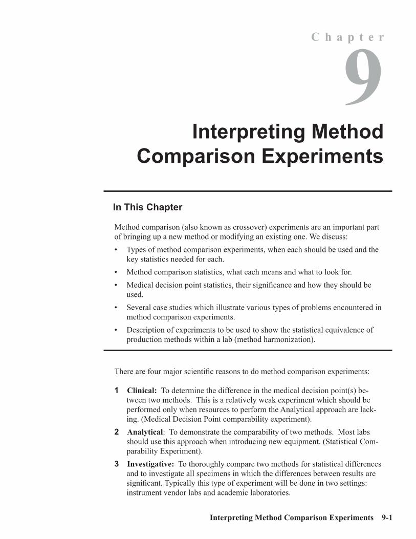
Interpreting Method Comparison Experiments 9-1
C h a p t e r
9Interpreting Method
Comparison Experiments
In This Chapter
Method comparison (also known as crossover) experiments are an important part of bringing up a new method or modifying an existing one. We discuss:• Types of method comparison experiments, when each should be used and the
key statistics needed for each.• Method comparison statistics, what each means and what to look for.• Medical decision point statistics, their significance and how they should be
used.• Several case studies which illustrate various types of problems encountered in
method comparison experiments.• Description of experiments to be used to show the statistical equivalence of
production methods within a lab (method harmonization).
There are four major scientific reasons to do method comparison experiments:
1 Clinical: To determine the difference in the medical decision point(s) be-tween two methods. This is a relatively weak experiment which should be performed only when resources to perform the Analytical approach are lack-ing. (Medical Decision Point comparability experiment).
2 Analytical: To demonstrate the comparability of two methods. Most labs should use this approach when introducing new equipment. (Statistical Com-parability Experiment).
3 Investigative: To thoroughly compare two methods for statistical differences and to investigate all specimens in which the differences between results are significant. Typically this type of experiment will be done in two settings: instrument vendor labs and academic laboratories.

9-2 Lab Statistics - Fun and Easy
4 Verification of Method Harmonization: To verify that results from multiple instruments already adopted are equivalent within a specified tolerance. This type of experiment is discussed at the very end of this chapter.
The only similarities among the first three approaches are: • Similar statistical calculations. • Assay of specimens by two or more methods.
The differences between these three approaches include: • The numbers of specimens involved• The range of specimens used • The nature of the specimens used • The quality of the X (comparative) method • The diligence used in tracking down the reasons for significant differences
between results
Interpretation of Method Comparison Results
Keep the following in mind as you design experiments or review Method Com-parison reports:• All results are relative. Unless one method is a Definitive Method (i.e. a high-
ly defined, extremely accurate and precise method), the reference (X) method will likely be imperfect. When changing methods, the new (Y) method is often better than the old (X) method.
• The specimens chosen can profoundly affect the experiment. • Specimen integrity. Unstable analyte concentrations (CPK, CO2, Na) may
compromise the results because the methods may not see the same concentra-tion.
• The concentration range of the specimens greatly influences the results. The greater the range within appropriate limits, the better the results.
• Data quality is important. Data from an out-of-control run will compromise the conclusions. Garbage in, garbage out.
Additionally, keep in mind that various statistics are indicators of two very differ-ent issues: • Quality of Data (QOD): Are the data capable of telling a reasonable
story? This indicates the care with which the experiment was performed. It includes: specimen selection leading to good range of results, freshness of specimens and the overall analytical quality of the experiment.
• Identity of Methods (IOM): What is the story that is being told by these data? These are the statistics (slope, intercept, etc.) by which the method is judged. Clearly they are strongly affected by the Quality of Data.

Interpreting Method Comparison Experiments 9-3
Point of the Experiment
One fundamental purpose of a method comparison experiment is to show that two methods are statistically equivalent. One can validly make this claim if three conditions are met:• The slope is not significantly different from 1.0 (usually).• The intercept is not significantly different from 0.0.• There is no significant difference in the medical decision points. The differences between two methods appear in one or more of the five general ways listed below.
• Constant Bias: differences between sets of results which are constant at all concentrations. (Non-zero intercept)
• Proportional Bias: differences between sets of results which are proportional to the analyte concentration. (Slope significantly different from one.)
• Random error: differences between results due to random effects. (Impreci-sion or other methodological error.)
• Patterns such as nonlinear results or outliers.• Other systematic problems such as selective interference or matrix effects.

9-4 Lab Statistics - Fun and Easy
Concepts and Definitions
The two general types of calculations done for method comparison studies are linear regression and dispersion of data around a central tendency.
The sensitivity of the major statistical parameters is shown in Table 9.1. Each of these parameters is discussed in detail. This table is derived from a similar table in Westgard and Hunt (1973).
Table 9.1Sensitivity of Statistical Parameters
to Three Classes of ErrorRandom Proportional Constant
Slope No Yes NoIntercept No No YesStd. Err. Est. Yes No NoBias No Yes YesStd. Dev. Diff Yes Yes Yest Test Yes Yes YesCorr. Coef. (R)* Yes No NoMed. Dec. Pt. No No NoPredicted Bias No Yes Yes95% Conf. Limits Yes Yes Yes
*Corr. Coef. (R) is also sensitive to the range of the results.
Concept: Data Distributions
These concepts describe the populations of the results for each method. In gen-eral, these statistics indicate the Quality of Data.
Result Ranges show the actual ranges of the results for the two methods. X Mean and SD are the average (cen-tral tendency) and SD (dispersion) of the data plotted on the X axis. In the figure at right, they correspond to the RIA data and describe the distribution of those results.
X Mean and SD are the average (cen-tral tendency) and SD (dispersion) of the data plotted on the X axis. In the figure at right, they correspond to the RIA data and describe the distribution of those results.
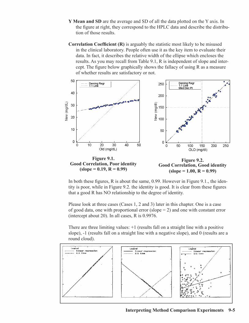
Interpreting Method Comparison Experiments 9-5
Y Mean and SD are the average and SD of all the data plotted on the Y axis. In the figure at right, they correspond to the HPLC data and describe the distribu-tion of those results.
Correlation Coefficient (R) is arguably the statistic most likely to be misused in the clinical laboratory. People often use it as the key item to evaluate their data. In fact, it describes the relative width of the ellipse which encloses the results. As you may recall from Table 9.1, R is independent of slope and inter-cept. The figure below graphically shows the fallacy of using R as a measure of whether results are satisfactory or not.
In both these figures, R is about the same, 0.99. However in Figure 9.1., the iden-tity is poor, while in Figure 9.2. the identity is good. It is clear from these figures that a good R has NO relationship to the degree of identity.
Please look at three cases (Cases 1, 2 and 3) later in this chapter. One is a case of good data, one with proportional error (slope = 2) and one with constant error (intercept about 20). In all cases, R is 0.9976.
There are three limiting values: +1 (results fall on a straight line with a positive slope), -1 (results fall on a straight line with a negative slope), and 0 (results are a round cloud).
Figure 9.1.Good Correlation, Poor identity
(slope = 0.19, R = 0.99)
Figure 9.2.Good Correlation, Good identity
(slope = 1.00, R = 0.99)

9-6 Lab Statistics - Fun and Easy
R is sensitive to random error, to the range of the data and to the sign of the slope, not the slope or intercept. R is a measure of the range of the data relative to the random error. If the SD stays constant as the range of data increases, R will increase and will gradually approach 1. Case 8: Effect of Range of Results later in this chapter illustrates the effect of range on R.
R is used to determine which type of calculation should be used for the Predicted Medical Decision point and the associated 95% Confidence Limits. If R is less than 0.90 (for the Alternate module) or 0.975 (for EP9), then these items are cal-culated using the Partitioned Bias Procedure. Otherwise they are calculated from Deming linear regression statistics.
This is a “quality of data” statistic, not the “quality of method” statistic. A high number indicates that a good range of data is present and that more weight can be placed on the experimental results.
Keep in mind that different R values are expected for each analyte. Many chemis-try analytes, such as LDH and glucose, have R values of 0.98 and higher because they have wide ranges. For other analytes with narrower ranges, such as the electrolytes, sodium and chloride, and several hematology cell differential param-eters, R values typically are much lower. For sodium, neutrophils and basophils, R values of 0.90, 0.80 and 0.30, respectively, are common.
One other aspect of R needs to be kept in mind. That is expressed by the follow-ing approximate relationship (shown in the equation below) which holds when the errors of the two methods are similar and R is greater than 0.8:
Corr. Coef (R) = Regular slope / Deming slope
One major implication of this relationship is that the Regular slope is always less than the Deming slope. In all the experiments that I have simulated, the Deming slope is a much better approximation of the target (true) slope. Consequently, the Regular slope always underestimates the true slope. The only issue is by how much.
A second implication is that if R has a value of 0.995, then the difference between the slopes (0.5%) is insignificant in most cases. In this case, it probably doesn’t matter whether the Regular or Deming slope is used. On the other hand, if R is 0.90, then the difference between the slopes (10%) probably is significant. In this case, the Deming slope must be used.

Interpreting Method Comparison Experiments 9-7
Concept: Bias
The terms listed below describe statistically the differences between pairs of re-sults i.e. yi, xi where xi and yi are the values of the ith pair results for the X and Y methods. In general, these are Quality of Method statistics.
Bias has several definitions:
• Ymean - Xmean. (best definition)• The differences between individual pairs of results (yi - xi).• A casual reference to systematic error.
Standard Deviation of the Differ-ences (SDD) is the standard devia-tion (dispersion) of the differences between pairs of results. The bias plot graphs this statistic. The SDD is represented by the envelope of dispersion lines around the bias.
t Test is calculated from an equation which has bias in the numerator and SDD in the denominator. t Probabil-ity corresponds to the number normally looked up in the t test table. It is the probability that the bias can be accounted for by the SDD. It is not meaning-ful when the slope is outside the range of 0.9 to 1.1. If the t test is used, it is significant at the 95% confidence level if the t Probability is less than 0.05. Of all the statistics presented in this module, the t test is the weakest.
A sound bite for the t test is “He who lives by the t test, dies by the t test.” In the case studies at the end of this chapter, check the number of cases in which the t test indicates problems and the number it misses.
Bias plots are useful because they show the relationships of the differences be-tween two different results. Outliers are obvious in the plot. Subtle patterns can show the presence of problems. For example, a group of results significantly removed from the others could indicate that one instrument was out of control on a certain day. Other patterns show the presence of non-linear assays (Case 5: Non-Linear Pattern), random error (Case 4: Effect of Random Error), constant bias (Case 3: Effect of Constant Error). With the default plotting approach of EP Evaluator®, a bias plot for a good case is a round cloud.
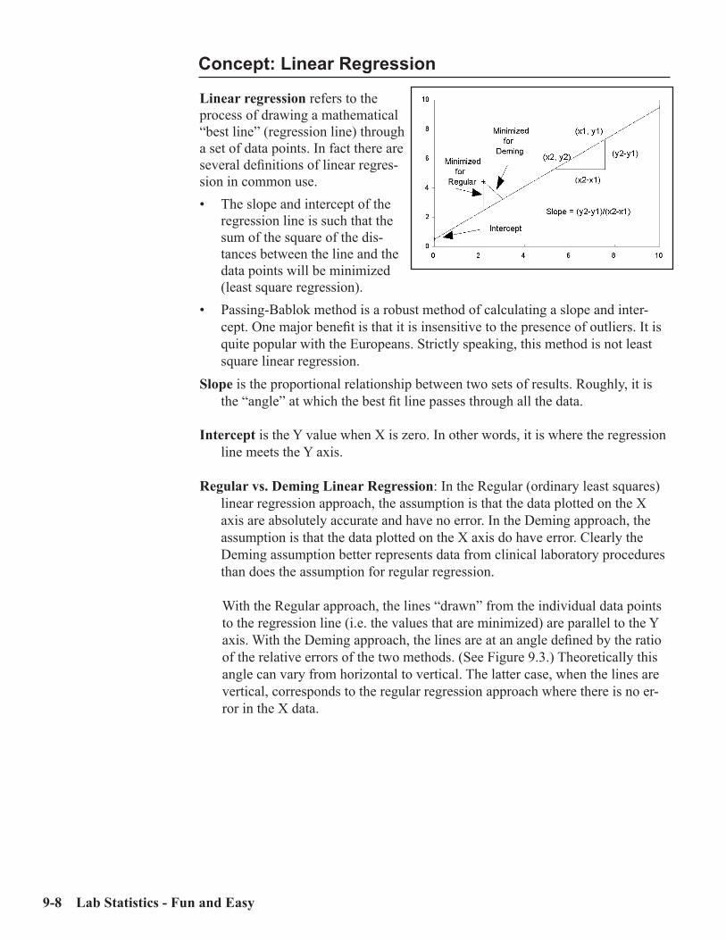
9-8 Lab Statistics - Fun and Easy
Concept: Linear Regression
Linear regression refers to the process of drawing a mathematical “best line” (regression line) through a set of data points. In fact there are several definitions of linear regres-sion in common use.• The slope and intercept of the
regression line is such that the sum of the square of the dis-tances between the line and the data points will be minimized (least square regression).
• Passing-Bablok method is a robust method of calculating a slope and inter-cept. One major benefit is that it is insensitive to the presence of outliers. It is quite popular with the Europeans. Strictly speaking, this method is not least square linear regression.
Slope is the proportional relationship between two sets of results. Roughly, it is the “angle” at which the best fit line passes through all the data.
Intercept is the Y value when X is zero. In other words, it is where the regression line meets the Y axis.
Regular vs. Deming Linear Regression: In the Regular (ordinary least squares) linear regression approach, the assumption is that the data plotted on the X axis are absolutely accurate and have no error. In the Deming approach, the assumption is that the data plotted on the X axis do have error. Clearly the Deming assumption better represents data from clinical laboratory procedures than does the assumption for regular regression.
With the Regular approach, the lines “drawn” from the individual data points to the regression line (i.e. the values that are minimized) are parallel to the Y axis. With the Deming approach, the lines are at an angle defined by the ratio of the relative errors of the two methods. (See Figure 9.3.) Theoretically this angle can vary from horizontal to vertical. The latter case, when the lines are vertical, corresponds to the regular regression approach where there is no er-ror in the X data.
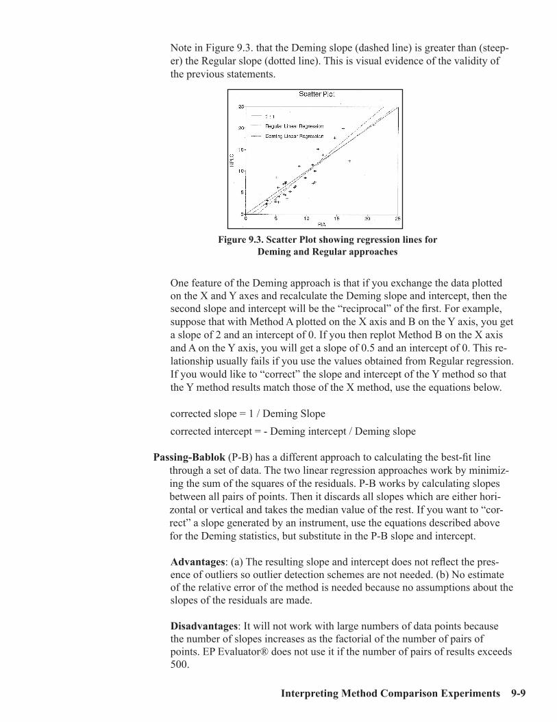
Interpreting Method Comparison Experiments 9-9
Note in Figure 9.3. that the Deming slope (dashed line) is greater than (steep-er) the Regular slope (dotted line). This is visual evidence of the validity of the previous statements.
One feature of the Deming approach is that if you exchange the data plotted on the X and Y axes and recalculate the Deming slope and intercept, then the second slope and intercept will be the “reciprocal” of the first. For example, suppose that with Method A plotted on the X axis and B on the Y axis, you get a slope of 2 and an intercept of 0. If you then replot Method B on the X axis and A on the Y axis, you will get a slope of 0.5 and an intercept of 0. This re-lationship usually fails if you use the values obtained from Regular regression. If you would like to “correct” the slope and intercept of the Y method so that the Y method results match those of the X method, use the equations below.
corrected slope = 1 / Deming Slopecorrected intercept = - Deming intercept / Deming slope
Passing-Bablok (P-B) has a different approach to calculating the best-fit line through a set of data. The two linear regression approaches work by minimiz-ing the sum of the squares of the residuals. P-B works by calculating slopes between all pairs of points. Then it discards all slopes which are either hori-zontal or vertical and takes the median value of the rest. If you want to “cor-rect” a slope generated by an instrument, use the equations described above for the Deming statistics, but substitute in the P-B slope and intercept.
Advantages: (a) The resulting slope and intercept does not reflect the pres-ence of outliers so outlier detection schemes are not needed. (b) No estimate of the relative error of the method is needed because no assumptions about the slopes of the residuals are made.
Disadvantages: It will not work with large numbers of data points because the number of slopes increases as the factorial of the number of pairs of points. EP Evaluator® does not use it if the number of pairs of results exceeds 500.
Figure 9.3. Scatter Plot showing regression lines for Deming and Regular approaches

9-10 Lab Statistics - Fun and Easy
95% Confidence Intervals are the numbers in parentheses displayed on the Re-gression Analysis report shown below following the slope and intercept values and represent the range in values that would be expected 95% of the time were a similar experiment to be performed on a similar set of specimens.
95% confidence intervals are useful because they allow a statement of statisti-cal confidence to be made. Determine if the item (i.e. slope or intercept) is within the 95% confidence limits. Since the Deming slope of 1.007 is within the interval of 0.980 to 1.034, one can make a statement that:
“The slope is statistically equivalent to 1.0 with 95% confidence.” That is a much stronger statement than looking at the Deming slope of 1.007 and saying that it looks “pretty good.”
Standard Error of the Estimate (SEE) escribes the dispersion of the x,y points around the regression line (central tendency). The smaller the SEE, the better the results correlate. The relationship of the SEE to the regression line is shown above. If the random errors for both methods are identical, the SEE will be ap-proximately 1.4 times a typical SD. SEE is a measure of dispersion. The corresponding central tendency is the regression line.
SMAD (Scaled Median Absolute Deviation) is a value similar to Standard Error of the Estimate (SEE) in that it describes the scatter around best fit line, but developed with particular relevance to the Passing-Bablok approach as it is insensitive to outliers.

Interpreting Method Comparison Experiments 9-11
Concept: Representative SD
The fundamental difference between Regular and Deming linear regression is that Regular regression assumes that there is NO error in the data plotted on the X axis. In contrast, Deming regression assumes that the X data do contain error.
The problem is how to define the magnitude of the error. The way we have chosen to do it in EP Evaluator® is with the term of Representative SD. This is a single number which represents the average error profile of this method. In general, if two relatively similar instruments are being compared, the Rep SD’s can both be set to 1.0.
Of interest is how various regression statistics change as the Rep SD varies over a wide range. Note that the Regular slope is to 3 significant figures identical with the Rep SD Ratio of 10,000.
The statistics are much more sensitive to differences in Rep SD’s when R is relatively low. In the table below, for the data with the broad range (50 to 250), the total difference in the Deming slope is about 2% (0.98 to 1.00) over a range of values exceeding 1,000,000. For the narrow range data (70 to 100), the corre-sponding difference exceeds 30% (0.84 to 1.14).
Rep SD(Ratio Y/X)
TargetRange
DemingSlope
DemingIntercept
Corr. Coef.(R)
10,000 50 to 250 0.982 1.6 0.98971 50 to 250 0.992 0.0 0.9897
0.0001 50 to 250 1.002 -1.5 0.989710,000 70 to 100 0.844 12.7 0.8591
1 70 to 100 0.980 1.0 0.85910.0001 70 to 100 1.143 -13.0 0.8591
The Regular slope was 0.982 for the first case (50 to 250) and 0.844 for the second (70 to 100).

9-12 Lab Statistics - Fun and Easy
Concept: Scatter Plot Bounds
Scatter Plot Bounds define an area between two boundaries drawn around ei-ther the regression or identity line and within which the experimental results are expected to fall most of the time. The major purpose of Scatter Plot Bounds is to show graphically which points are outliers. The three types of Scatter Plot Bounds supported in EP Evaluator® are illustrated in the figure at below.
95% Confidence Interval: This popular feature which is often applied to many quantitative analytes has two major weaknesses: a) Since it calculated from the experimental data, its shape and position change depending on the qual-ity of the data. For example, if an outlier is present, the bounds can expand dramatically. Consequently it provides little help to the user in a regulatory environment which specifies total allowable error for many analytes; b) The curve has a slightly convex shape which is closest to the regression line near the center of the results and then flares gently outwards at both ends. As a result, it often does a poor job of detecting outliers especially at the low end of the curve.
Allowable error: Its advantages are that it is independent of scatter in the experi-mental data. Consequently it allows the user to judge the quality of the data against a predefined standard. Unlike the 95% CI above, it does not change its position relative to the regression line when presented with poor data. Its shape is defined by the amount of allowable error, either concentration, per-cent concentration or both. It is plotted around the Deming regression line.
White cell differential counts. Also known as the binomial distribution: The scatter plot bounds are based on the statistical uncertainty for counting cells. More specifically, it represents the error in finding the “true” fraction in the limited population that was sampled which usually is the 100 or 200 cells that were counted manually vs. the 10,000 or so that were counted by an instru-ment. This approach is independent of the experimental data. The shape of the bounds is concave and the bounds are centered on the identity (1:1) line. One expects 5% of the points to be outside these bounds.
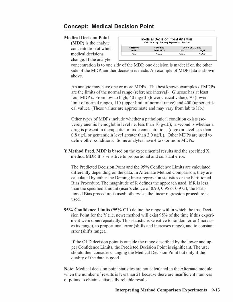
Interpreting Method Comparison Experiments 9-13
Concept: Medical Decision Point
Medical Decision Point (MDP) is the analyte concentration at which medical decisions change. If the analyte concentration is to one side of the MDP, one decision is made; if on the other side of the MDP, another decision is made. An example of MDP data is shown above.
An analyte may have one or more MDPs. The best known examples of MDPs are the limits of the normal range (reference interval). Glucose has at least four MDP’s. From low to high, 40 mg/dL (lower critical value), 70 (lower limit of normal range), 110 (upper limit of normal range) and 400 (upper criti-cal value). (These values are approximate and may vary from lab to lab.)
Other types of MDPs include whether a pathological condition exists (se-verely anemic hemoglobin level i.e. less than 10 g/dL); a second is whether a drug is present in therapeutic or toxic concentrations (digoxin level less than 0.8 ug/L or gentamicin level greater than 2.0 ug/L). Other MDPs are used to define other conditions. Some analytes have 4 to 6 or more MDPs.
Y Method Pred. MDP is based on the experimental results and the specified X method MDP. It is sensitive to proportional and constant error.
The Predicted Decision Point and the 95% Confidence Limits are calculated differently depending on the data. In Alternate Method Comparison, they are calculated by either the Deming linear regression statistics or the Partitioned Bias Procedure. The magnitude of R defines the approach used. If R is less than the specified amount (user’s choice of 0.90, 0.95 or 0.975), the Parti-tioned Bias procedure is used; otherwise, the linear regression procedure is used.
95% Confidence Limits (95% CL) define the range within which the true Deci-sion Point for the Y (i.e. new) method will exist 95% of the time if this experi-ment were done repeatedly. This statistic is sensitive to random error (increas-es its range), to proportional error (shifts and increases range), and to constant error (shifts range).
If the OLD decision point is outside the range described by the lower and up-per Confidence Limits, the Predicted Decision Point is significant. The user should then consider changing the Medical Decision Point but only if the quality of the data is good.
Note: Medical decision point statistics are not calculated in the Alternate module when the number of results is less than 21 because there are insufficient numbers of points to obtain statistically reliable results.

9-14 Lab Statistics - Fun and Easy
Types of Method Comparison Experiments
The most important statistical parameters depend on the purpose of the experi-ment.
Clinical When the purpose is clinical, generally the decision has already been made by the laboratory to adopt the method or instrument. The issue is whether the medical decision point (MDP) should be changed. The most important parameters to con-sider are the 95% CL for the MDP. They indicate whether the MDP for the new method is significantly different from that for the old method. If the OLD MDP is between the lower and upper 95% CL, this experiment does not support changing the MDP. If the OLD MDP is outside the range of the 95% CL, this is evidence that the MDP should be changed. If so, one needs to proceed cautiously and gather more information.
First one should assay a substantially larger number of specimens to confirm one’s initial results. If you do confirm that there is a significant difference between the OLD and NEW MDP’s, then you must re-establish the MDP.
Changing a medical decision point IS A BIG DEAL!!! Do not make changes lightly. If the MDP changes, the lab’s clients and physicians MUST BE NOTI-FIED when the changes become effective.
AnalyticalWhen the purpose is analytical, the issue is whether the two methods are statisti-cally equivalent. Here the slope and intercept and their 95% CIs and the 95% CL of the MDP are most important.
The 95% confidence interval for the slope and intercept is approximately the ±2 SD range. If 1.00 is between the lower and upper limits, one can say with 95% confidence that this slope is not different from a slope of 1.00.
Similarly, a 95% confidence interval can be calculated for the intercept. If 0.0 is between these two numbers, one can say with 95% confidence that this intercept is not different from an intercept of 0.0.
If two methods are calculated to be statistically equivalent, then their MDPs and reference ranges should also be statistically equivalent. If this is not the case, this discrepancy needs to be investigated.
Slope and intercept lose reliability when the correlation coefficient (R) is less than 0.95. There is too much scatter in the data to be able to draw statistically reliable conclusions from the linear regression data.
InvestigativeThe significance of the various parameters is beyond the scope of this work.

Interpreting Method Comparison Experiments 9-15
Interpretation of Results
The case studies below illustrate several types of problems which may be encoun-tered while doing method comparison studies.
Case StudiesCase 1: A Good ExampleCase 2: Effect of Proportional ErrorCase 3: Effect of Constant ErrorCase 4: Effect of Random ErrorCase 5: Non-Linear PatternCase 6: Effect of OutliersCase 7: Effect of Extreme RangeCase 8: Effect of Range of ResultsCase 9: Effect of Number of SpecimensCase 10: Effect of Poor Distribution of Results
The results used in these case studies were simulated. Unless otherwise indicated, the number of results is 50, the target slope is 1.0, the target intercept is 0.0, the target range is 50 to 250, the target CV is 2.0% and the medical decision point is 100. The calculated statistics are by the Deming method. The representative SDs were the defaults of 1.0. The Scatter Plot Bounds shown are calculated with a 6% allowable error.
How Results were Generated
The results used in these examples were obtained from a program which simulates output from a clinical laboratory instrument. The program contained a random number generator which output results in an approximate Gaussian distribution. Since the random number generator was started with the same seed in all cases, the same sequence of random numbers was generated for all cases where the num-ber of points were identical.
Input to the result generating program includes a slope and intercept, the upper and lower limits of the range of results before addition of the random error com-ponent, CVs for both the X and Y methods and the number of points to generate. The program generates a series of results at even intervals along the range. A random error component is then added to each of those results. The results for the nonlinear and outlier examples are arbitrarily “doctored” versions of the “good” set of results.
The results were then imported into EP Evaluator® through the rapid results entry facility using the Windows clipboard. Then the statistics were calculated.

9-16 Lab Statistics - Fun and Easy
Case 1: A Good Example
This case illustrates good data. An adequate number of results (50) are spread across a broad range (50 to 250). The slope is 1 and the intercept is 0 (both within 95% confidence limits). The bias is small compared to typical results. The SDD and SEE are about equal and the correlation coefficient is high (0.9976). At the MDP of 100 units, the bias is 0.2 and the 95% confidence limits for the MDPs are tight with a total range of 3.1 units.

Interpreting Method Comparison Experiments 9-17
Properties of Good Data
• Adequate number of points. A minimum of 25 points are present, preferably 40 to 80.
• Points are reasonably distributed across the range of the method.• The data fall close to a straight line. • Bias plot appears to be a round cloud and the mean bias is close to 0.0.• Number of outliers is small. In other words, this number does not exceed 2.5%
of the total number of points.• The slope is close to 1.0.
• 95% CI of the Deming slope includes the value of 1.0. In other words, 1.0 is not less than the lower limit, nor greater than the upper limit.
• The intercept is close to 0.0.• 95% CI of the Deming intercept includes the value of 0.0.
• The MDP’s for the X and Y values are not significantly different.
• The 95% CI of the MDP’s all include the X value MDP.• Almost all the results fall outside the scatter plot bounds defined by either Al-
lowable Error or Differential Cell Count whichever is appropriate.
Additional (much less important) tests:• Random error reflects what is normally observed for those methods.• Mean bias is approximately zero within 2 SDD’s.
If the above statements are all true, then you can make the powerful statement that the two methods are equivalent within 95% confidence.

9-18 Lab Statistics - Fun and Easy
Report for Good Case
Case 2: Effect of Proportional Error
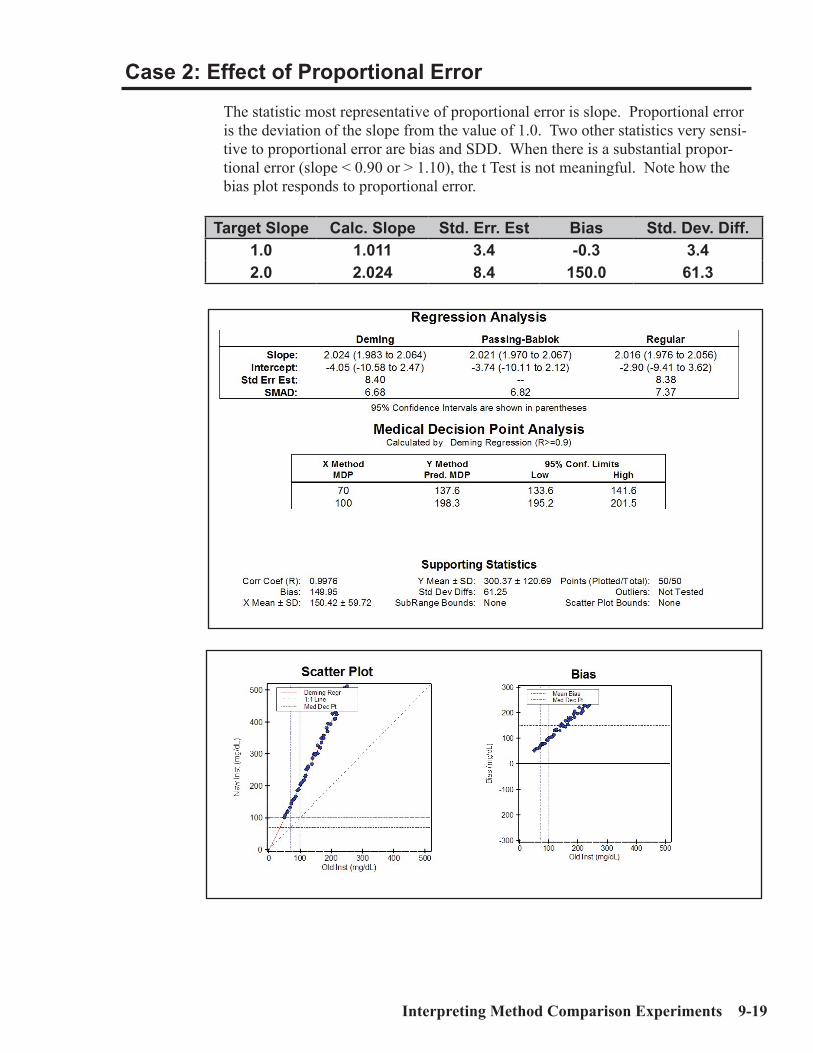
Interpreting Method Comparison Experiments 9-19
Case 2: Effect of Proportional Error
The statistic most representative of proportional error is slope. Proportional error is the deviation of the slope from the value of 1.0. Two other statistics very sensi-tive to proportional error are bias and SDD. When there is a substantial propor-tional error (slope < 0.90 or > 1.10), the t Test is not meaningful. Note how the bias plot responds to proportional error.
Target Slope Calc. Slope Std. Err. Est Bias Std. Dev. Diff.1.0 1.011 3.4 -0.3 3.42.0 2.024 8.4 150.0 61.3
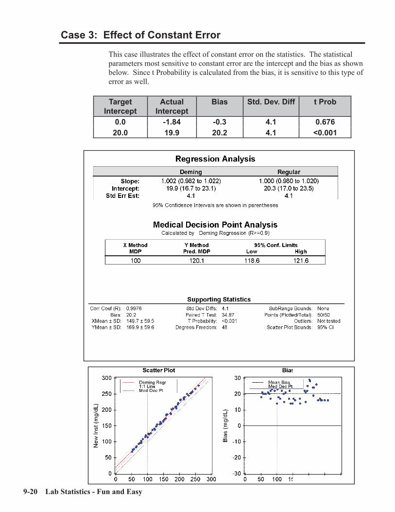
9-20 Lab Statistics - Fun and Easy
Case 3: Effect of Constant Error
This case illustrates the effect of constant error on the statistics. The statistical parameters most sensitive to constant error are the intercept and the bias as shown below. Since t Probability is calculated from the bias, it is sensitive to this type of error as well.
Target Intercept
Actual Intercept
Bias Std. Dev. Diff t Prob
0.0 -1.84 -0.3 4.1 0.67620.0 19.9 20.2 4.1 <0.001
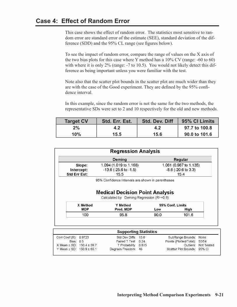
Interpreting Method Comparison Experiments 9-21
Case 4: Effect of Random Error
This case shows the effect of random error. The statistics most sensitive to ran-dom error are standard error of the estimate (SEE), standard deviation of the dif-ference (SDD) and the 95% CL range (see figures below).
To see the impact of random error, compare the range of values on the X axis of the two bias plots for this case where Y method has a 10% CV (range: -60 to 60) with where it is only 2% (range: -7 to 10.5). You would not likely detect this dif-ference as being important unless you were familiar with the test.
Note also that the scatter plot bounds in the scatter plot are much wider than they are with the case of the Good experiment. They are defined by the 95% confi-dence interval.
In this example, since the random error is not the same for the two methods, the representative SDs were set to 2 and 10 respectively for the old and new methods.
Target CV Std. Err. Est. Std. Dev. Diff 95% CI Limits2% 4.2 4.2 97.7 to 100.8
10% 15.5 15.6 90.0 to 101.6

9-22 Lab Statistics - Fun and Easy
Bias Plot - 2% CVBias Plot - 10% CV
Compare the scales!!

Interpreting Method Comparison Experiments 9-23
Case 5: Non-Linear Pattern
Non-linear patterns indicate the presence of problems. A common form is shown below where non-linearity shows up at the high end of the curve.
The easiest way to recognize non-linear systems is to look at the graphs. While it shows up on the scatter plot, it is most obvious on the bias plot. The slope in the report suggests that things aren’t quite right, but the effects there are subtle. A simple glance at the bias plot shows where the problem is immediately.
Note that if the highest value assayed had been 180 (vs. the actual 250), the non-linearity would not have been detected.

9-24 Lab Statistics - Fun and Easy
Case 6: Effect of Outliers
To understand outliers, one must realize that they can occur for many reasons such as a large random error, idiosyncratic error, or an effect caused by an inter-fering material.
When specimens are assayed in duplicate, outliers will be detected by the CLSI:EP9 protocol if a significant discrepancy occurs between duplicates. Alter-nate Method Comparison detects outliers if a residual (distance between the point and the regression line) is 10 or more times the median residual.
The effect of outliers is shown in the statistics shown below. The data is identical to that of Case 1, except that one point has been increased 50%. Blatant outliers are easy to spot on the graph. They have most effect on parameters which are indicators of random error such as SDD and SEE.
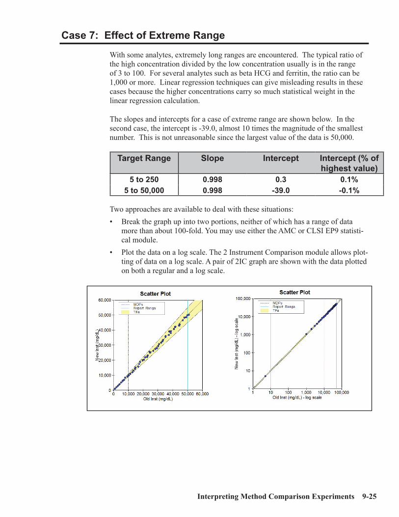
Interpreting Method Comparison Experiments 9-25
Case 7: Effect of Extreme Range
With some analytes, extremely long ranges are encountered. The typical ratio of the high concentration divided by the low concentration usually is in the range of 3 to 100. For several analytes such as beta HCG and ferritin, the ratio can be 1,000 or more. Linear regression techniques can give misleading results in these cases because the higher concentrations carry so much statistical weight in the linear regression calculation.
The slopes and intercepts for a case of extreme range are shown below. In the second case, the intercept is -39.0, almost 10 times the magnitude of the smallest number. This is not unreasonable since the largest value of the data is 50,000.
Target Range Slope Intercept Intercept (% of highest value)
5 to 250 0.998 0.3 0.1%5 to 50,000 0.998 -39.0 -0.1%
Two approaches are available to deal with these situations:• Break the graph up into two portions, neither of which has a range of data
more than about 100-fold. You may use either the AMC or CLSI EP9 statisti-cal module.
• Plot the data on a log scale. The 2 Instrument Comparison module allows plot-ting of data on a log scale. A pair of 2IC graph are shown with the data plotted on both a regular and a log scale.

9-26 Lab Statistics - Fun and Easy
Case 8: Effect of Range of Results
One common error is that the data has too narrow a range. This admittedly extreme case (see figures below) shows how poor results can get when the range is narrow (70 to 80), the number of specimens are few (12) and the SDs approxi-mates the range of the results.
The single statistic which points directly to the problems of these data is the Cor-relation Coefficient. The ONLY potentially positive item in these statistics is the bias. All statistics related to slope and intercept are worthless!!
This is an example of results which fail the Quality of Data test.
Target Range
Slope Intercept Corr. Coef Pred MDP
70-80 -1.021 151.7 -0.05 80.670-100 0.526 40.3 0.38 80.370-150 0.783 28.0 0.80 79.3
The number of results for all experiments was 12.The target CV’s for all methods were 10%.

Interpreting Method Comparison Experiments 9-27
Recommendations: • Make sure your data cover a reasonable range. The more you cover the report-
able range of your method the better. • Expand the range to improve the quality of your results. Use the bins feature
of the software to help you better judge the distribution of your data.Often it is difficult to collect results over a broad range. This may be because the patient population is almost all normal (outpatient laboratories) or the ana-lytes have a narrow range of results (sodium). In these cases, collect speci-mens with results that include the medical decision point(s). This will help make the average bias at the medical decision point more reliable. In some settings, it will be difficult to collect specimens with wide-ranging results. It may take a period of weeks or months to do this.
If the purpose of method comparison experiment is to match the output of two instruments, it is very important for the results to cover a broad analytical range. Otherwise, significant errors in the slope and intercept may occur. The user must make vigorous efforts to obtain a satisfactory set of specimens.

9-28 Lab Statistics - Fun and Easy
Case 9: Effect of Number of Specimens
The number of specimens used in the experiment is important. The problem with having too few specimens is that the usual random error affects the results sig-nificantly. The presence of larger numbers of specimens averages out the random error.
If the number of specimens is small, the quality of the statistics will be poor. The poor quality shows up as larger 95% confidence intervals for the slope and inter-cept and a larger range for the 95% confidence limits (95% CL) for the MDP.
N Slope Intercept 95% CL Range - MDP
12 0.96 (0.90 - 1.01) 4.2 (-1.4 to 9.8) 1.550 0.99 (0.97 to 1.02) 0.4 (-2.0 to 2.8) 1.4
The target range of the results in this talbe is 50 to 150.
In general, the range of the 95% CL tends to be inversely proportional to the square root of the number of specimens, assuming everything else remains con-stant. In other words, if the number of results quadruples, the 95% CL range decreases by a factor of about 2. It is each laboratory’s decision whether its 95% CL is satisfactory.
Recommendation:• The statistically rigorous and rugged CLSI EP9 protocol recommends that 40
specimens be assayed in duplicate for a total of 80 results. • For clinical laboratories, a minimum of 25 specimens should be used. Keep
in mind that a good distribution of results is more important than numbers of specimens. The quality of your experiment will be much better if you have results from 25 specimens spread over most of the reportable range than if you have 100 specimens all in the (relatively narrow) normal range.

Interpreting Method Comparison Experiments 9-29
Case 10: Effect of Poor Distribution of Results
In an extreme case, as shown below, most of the data are in the lower portion of the range. Only a single point is at the high end. The net result is that the slope and intercept of the experiment are profoundly affected by this single point. Fifty of the 51 points were in the target range of 70 to 100. The 51st point was either 400 or 500.
X Value Y Value Slope Intercept500 500 1.000 2.5500 500 0.765 3.2

9-30 Lab Statistics - Fun and Easy
Method Harmonization Experiment
This experiment is to be used to demonstrate that all methods use in a common LIS environment produce results which are clinically identical. The reason this is important is because it is virtually impossible to correctly interpret results for the same test if they are clinically different.
This type of method comparison experiment is very different from the types we have been discussing previously because it uses a different paradigm than the previous ones as shown below:
Linear Regression Approach: Purpose of experiment is to demonstrate the statistical identity of two methods. If they are different, the medical deci-sion point should be revised if this proposed method is adopted. The number of specimens preferred for this sort of experiment is 35 to 50. The statistical analysis generates the usual linear regression statistics.
Method Harmonization Approach: Purpose of experiment is to demonstrate whether two or more methods already adopted by a laboratory are clinically identical. The experiment consists of analyzing a set of specimens (Number of specimens may be from 4 to 10) covering a suitable portion of the reportable range. The differences between the individual results from each instrument and the target values are calculated. An experiment fails passes if more than 5% of those differences exceeds Total Allowable Error.
EP Evaluator® has two statistical modules for evaluating method harmonization. They are Two Instrument Comparison (2IC) and Multiple Instrument Compari-son. A key graph below from 2IC, plots the differences of the results from the two instruments versus the X results. Failure occurs when over 5% of the points are outside the colored band (i.e. those differences exceed Total Allowable Error).

Interpreting Linearity Experiments 10-1
C h a p t e r
10Interpreting Linearity Experiments
In This Chapter
Linearity-style experiments use specimens with defined concentrations of ana-lytes. We discuss:• Experiments to establish or verify accuracy, reportable range, and linearity.• Experiments to verify calibration.• CLSI EP10 experiments to do preliminary evaluation of linearity, accuracy,
precision, reportable range, carryover and drift on quantitative methods.• Interpretation of linearity-style experiments.• Definitions of terms used in conjunction with linearity-style experiments.
This chapter is provided to help you understand the information calculated using EP Evaluator®’s Linearity module. Linearity provides the facility of evaluating laboratory methods for any or all of the following:
Linearity: See definitions of linearity discussed in Linearity section below:Accuracy: The term used in the software is Percent Recovery. A method is accu-
rate if the observed means are all sufficiently close to the correct value.Reportable Range: The range of analytical results which can be reliably reported
without dilution of the specimen.Precision: A within-run precision analysis which is designed to be a quick ap-
proach to validating instrument precision.Calibration Verification: Determines whether the method is accurate (according
to the user’s specifications) throughout its reportable range.Probability of Proficiency Testing Failure allows the user to determine the
probability of failure of an analyte during proficiency testing. See Chapter 11, Understanding Proficiency Testing for details.

10-2 Lab Statistics - Fun and Easy
Definition of Some Statistical Terms
Best Fit Line is calculated in one of two ways depending on whether an allow-able error is input or not. If allowable error is defined and linearity is selected, then the best fit line is obtained using the clinical linearity algorithm; other-wise it is calculated using regular linear regression.
Slope is the angle of the best fit line through the results. The ideal slope is 1.00.Intercept is the value on the Y axis at which the best fit line intersects. The ideal
intercept is zero.Std Err Est (Standard Error of the Estimate) is a measure of the dispersion of the
data points around the linear regression line. Used only with linear regression.Observed Error is the minimum allowable error which could be defined for a
data set and still have it be linear. Used only with Clinical Linearity.Proximity Limits are the user-defined acceptable limits for the concentration of
the specimens used to test the reportable range. If that concentration is within the proximity limits, then the method passes one part of the two part test for meeting the manufacturer’s claim for the reportable range.
Residual is the difference between the best fit line and a result. For example, if the slope and intercept of a best fit line are 1.1 and +10, and a result of 55 is obtained for a specimen with a defined concentration (defConc) of 50, the residual is:
residual = result - (slope * defConc + intercept) = 55 - (1.1 * 50 + 10) = 55 - 65 = -10 Recovery is the percent difference between a measured result and the assigned
value. It is a measure of the accuracy in the analytical process. For example, if a result of 4.5 was obtained for a specimen with a value of 5.0, 90% recovery was achieved.
Allowable Error and Error Budgets are discussed in Chapter 5, Understanding Error and Performance Standards.
Linearity
One of the fundamental problems with Linearity studies at the time of this writing (Summer, 2005) is that there is no consensus within the clinical laboratory indus-try concerning either how to determine whether a set of data are linear or whether determination of linearity even is necessary. One reason for this is that until the advent of Clinical Linearity, a module unique to EP Evaluator®, no definition of linearity took allowable error into account.

Interpreting Linearity Experiments 10-3
Several definitions of linearity which have been used in the clinical laboratory industry include those below.
• A data set is linear if it looks linear. (Eyeball Definition)
• A data set is linear if a straight line can be drawn through all the points. (Pen-cil Width Definition)
• A data set is linear if the fitted polynomial curve is not significantly different from the “ideal” linear equation. Other qualifiers are also applied. (Polynomial Regression Definition) (CLSI:EP6 and CAP (1993)).
• A data set is linear if a straight line can be drawn through vertical error bars centered on the mean of the results for each specimen. The lengths of the ver-tical error bars are calculated from the user defined allowable error. (Clinical Linearity Definition) (Rhoads and Castaneda-Mendez - 1994)
We believe that the last of these definitions, that of Clinical Linearity, makes most sense in a laboratory setting because it is the only one that relates linearity to a user defined allowable error.
EP Evaluator® implements two general approaches for calculating Linearity. If Total Allowable Error (TEa) is not defined, a traditional linear regression ap-proach is used and the linearity decision is made by the user employing what-ever criteria the user deems appropriate (Traditional Linearity). If Linearity is selected, then the linearity decision is made by the software using our innovative Clinical Linearity algorithm.
Traditional (Pencil Width) Linearity
Historically, the determination of linearity has involved several steps. The first is to calculate the slope and intercept of the best fit line using least square linear regression. The second step is to look at the data and determine visually if it is acceptably linear. The third step, required if the data are not visually linear, in-volves calculation of the residuals (differences between the Y point and the linear regression line) and checking to see if they seem satisfactory.
Advantages: • Traditionally accepted in the industry; • Easy to calculate statistics (slope, intercept and standard error of the estimate
(SEE)). Disadvantages:• Unable to clearly define what constitutes linearity; • Unable to determine which points are outliers; • Unable to relate linearity to a user defined analytical goal; • Slope and intercept of best fit line may be biased if outliers are present.

10-4 Lab Statistics - Fun and Easy
Polynomial Regression Linearity
CLSI approved CLSI:EP6 in 2003. The protocol in this document is similar but not identical to that used by the CAP for their linearity surveys. In both cases, both linear and polynomial curves are fitted to the data using ordinary least squares regression. The differences arise from the way assigned concentrations for each specimen is defined, the criteria for linearity, and how non-linearity is described.
Advantages:• Approved by CLSI and CAP.• Required by the FDA for certain submissions.
Disadvantages:• Can incorrectly declare a case non-linear when Allowable Error criterion is
stated in percent and lower limit of data is near zero. (EP6A)• Non-linear descriptions are hard to understand. (CAP)• Identifies outliers, but does not exclude them. (Both)
Clinical Linearity
This is the only algorithm in commercially available software which can deter-mine whether a set of results is linear within a user defined allowable error (Ea). The functional definition of Clinical Linearity has three steps:
Entry of Allowable Error: The user enters an Ea such as CLIA PT limits for each method. Ea is expressed in units of concentration or percent of concen-tration or both.
Error Bars: Vertical error bars for each linearity specimen are calculated from the Ea. Each error bar is centered on the mean of the results for that specimen.
Determines Linearity: Our innovative algorithm attempts to draw a straight line through the error bars. If such a straight line can be drawn, then the user can claim that the data set is linear within the Ea.
Two additional steps provide additional data:• Detect and Exclude Outliers: If the system is non-linear, the program looks
for and excludes outliers one by one from the data set. The process of exclud-ing outliers continues until the remaining points are linear within the allow-able error or until results for only three specimens remain. Outliers may be anywhere in the data set including the middle points.
• Calculation of Best Fit Line: Several statistics are based on the best fit line which is calculated by iteratively adjusting an internal Ea value until only one line can be drawn through the error bars. The intrinsic error is the internal Ea of the best fit line. The slope and intercept are those of the best fit line.
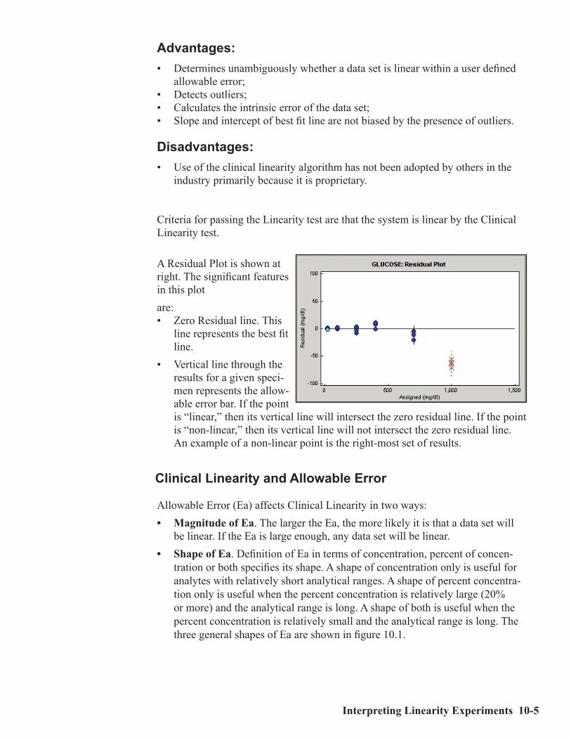
Interpreting Linearity Experiments 10-5
Advantages:• Determines unambiguously whether a data set is linear within a user defined
allowable error;• Detects outliers;• Calculates the intrinsic error of the data set;• Slope and intercept of best fit line are not biased by the presence of outliers.
Disadvantages:• Use of the clinical linearity algorithm has not been adopted by others in the
industry primarily because it is proprietary.
Criteria for passing the Linearity test are that the system is linear by the ClinicalLinearity test.
A Residual Plot is shown at right. The significant features in this plotare:• Zero Residual line. This
line represents the best fit line.
• Vertical line through the results for a given speci-men represents the allow-able error bar. If the point is “linear,” then its vertical line will intersect the zero residual line. If the point is “non-linear,” then its vertical line will not intersect the zero residual line. An example of a non-linear point is the right-most set of results.
Clinical Linearity and Allowable Error
Allowable Error (Ea) affects Clinical Linearity in two ways:• Magnitude of Ea. The larger the Ea, the more likely it is that a data set will
be linear. If the Ea is large enough, any data set will be linear.• Shape of Ea. Definition of Ea in terms of concentration, percent of concen-
tration or both specifies its shape. A shape of concentration only is useful for analytes with relatively short analytical ranges. A shape of percent concentra-tion only is useful when the percent concentration is relatively large (20% or more) and the analytical range is long. A shape of both is useful when the percent concentration is relatively small and the analytical range is long. The three general shapes of Ea are shown in figure 10.1.
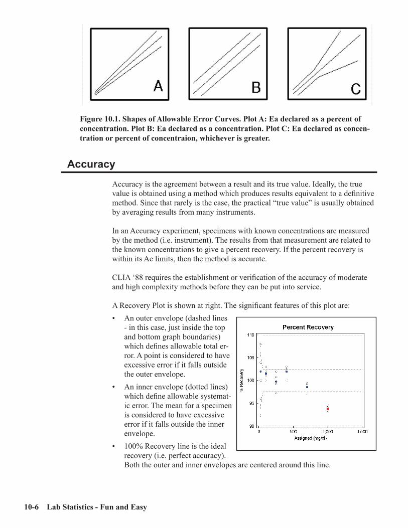
10-6 Lab Statistics - Fun and Easy
Accuracy
Accuracy is the agreement between a result and its true value. Ideally, the true value is obtained using a method which produces results equivalent to a definitive method. Since that rarely is the case, the practical “true value” is usually obtained by averaging results from many instruments.
In an Accuracy experiment, specimens with known concentrations are measured by the method (i.e. instrument). The results from that measurement are related to the known concentrations to give a percent recovery. If the percent recovery is within its Ae limits, then the method is accurate.
CLIA ‘88 requires the establishment or verification of the accuracy of moderate and high complexity methods before they can be put into service.
A Recovery Plot is shown at right. The significant features of this plot are:• An outer envelope (dashed lines
- in this case, just inside the top and bottom graph boundaries) which defines allowable total er-ror. A point is considered to have excessive error if it falls outside the outer envelope.
• An inner envelope (dotted lines) which define allowable systemat-ic error. The mean for a specimen is considered to have excessive error if it falls outside the inner envelope.
• 100% Recovery line is the ideal recovery (i.e. perfect accuracy). Both the outer and inner envelopes are centered around this line.
Figure 10.1. Shapes of Allowable Error Curves. Plot A: Ea declared as a percent of concentration. Plot B: Ea declared as a concentration. Plot C: Ea declared as concen-tration or percent of concentraion, whichever is greater.
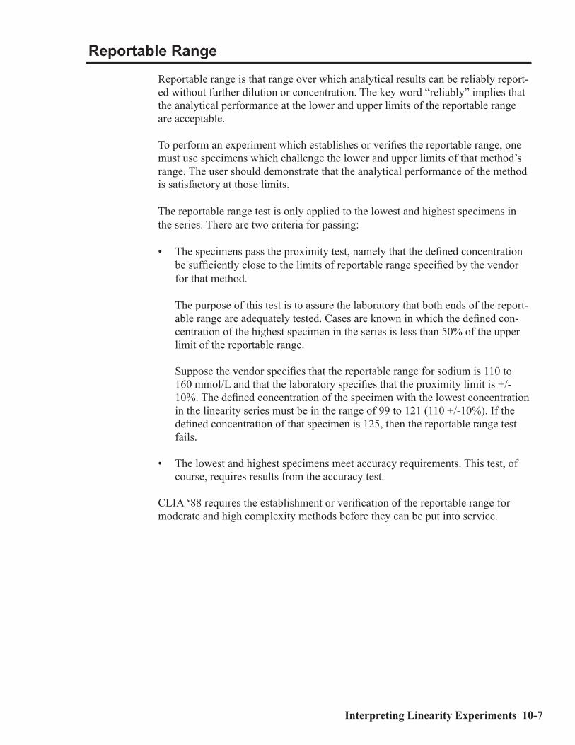
Interpreting Linearity Experiments 10-7
Reportable Range
Reportable range is that range over which analytical results can be reliably report-ed without further dilution or concentration. The key word “reliably” implies that the analytical performance at the lower and upper limits of the reportable range are acceptable.
To perform an experiment which establishes or verifies the reportable range, one must use specimens which challenge the lower and upper limits of that method’s range. The user should demonstrate that the analytical performance of the method is satisfactory at those limits.
The reportable range test is only applied to the lowest and highest specimens in the series. There are two criteria for passing:
• The specimens pass the proximity test, namely that the defined concentration be sufficiently close to the limits of reportable range specified by the vendor for that method.
The purpose of this test is to assure the laboratory that both ends of the report-able range are adequately tested. Cases are known in which the defined con-centration of the highest specimen in the series is less than 50% of the upper limit of the reportable range.
Suppose the vendor specifies that the reportable range for sodium is 110 to 160 mmol/L and that the laboratory specifies that the proximity limit is +/- 10%. The defined concentration of the specimen with the lowest concentration in the linearity series must be in the range of 99 to 121 (110 +/-10%). If the defined concentration of that specimen is 125, then the reportable range test fails.
• The lowest and highest specimens meet accuracy requirements. This test, of course, requires results from the accuracy test.
CLIA ‘88 requires the establishment or verification of the reportable range for moderate and high complexity methods before they can be put into service.

10-8 Lab Statistics - Fun and Easy
Calibration Verification
Calibration Verification is a reality check for whether a method can reliably mea-sure the concentration of the analyte throughout the reportable range. CLIA ‘88 requires that calibration verification experiments be performed at least once every six months as well as when significant maintenance events occur.
Calibration verification is defined as assaying three specimens. Two specimens must challenge the lower and upper limits of the reportable range respectively. The third should be near the mid-point.
In other words, the lab must verify the accuracy and reportable range of each method periodically. This experiment is identical to the CAP requirement of Veri-fying the Analytical Measurement Range. This current requirement represents a significant change from the regulations promulgated in 1992.
Case Studies
These cases are real linearity experiments. Results were obtained during the initial validation of an instrument. They illustrate a number of the issues that will be encountered during the method validation process.
Case 1: A Non-Linear CaseCase 2: Inaccurate ResultsCase 3: Failures Due to Inappropriate Specifications

Interpreting Linearity Experiments 10-9
Case 1: A Non-Linear Case
Results, statistical output and graphs for a Salicylate experiment are shown below. The total allowable error is 20%. Systematic error budget was 50%. To see the specifications, see the User Specifications Table below.
Case Analysis• Results are clearly non-linear.• Recovery is poor throughout the reportable range. Of the six specimens, two
are declared to be accurate. Four are considered to be linear.• If a concentration component (5 mg/dL in this case) is added to the TEa, the
accuracy and linearity problems with the lowest specimen are fixed. However those problems with the highest specimen still remain.
• Clearly there are severe systematic problems for this assay which need to be resolved.

10-10 Lab Statistics - Fun and Easy
Case 2: Inaccurate Results
This case (for Sodium) in which the results for all the specimens are significantly inaccurate is not uncommon. TEa is set to the CLIA ‘88 limits of 4 mmol/L. Sys-tematic error budget was 50%.
Case Analysis• All the results in this case seem to fall about 5 to 7 units below their assigned
values. This seems to be an example of constant error.• To fix it, one would proceed through the usual trouble-shooting process of
repeating analysis of the existing specimens, preparation of fresh linearity and calibration specimens followed by a re-calibration and re-assay of the linearity specimens. If those measures fail, then an examination of the instrument is in order.
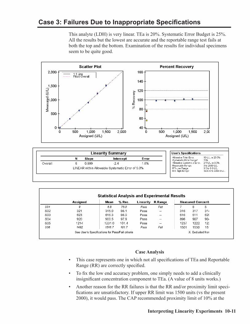
Interpreting Linearity Experiments 10-11
Case 3: Failures Due to Inappropriate Specifications
This analyte (LDH) is very linear. TEa is 20%. Systematic Error Budget is 25%. All the results but the lowest are accurate and the reportable range test fails at both the top and the bottom. Examination of the results for individual specimens seem to be quite good.
Case Analysis• This case represents one in which not all specifications of TEa and Reportable
Range (RR) are correctly specified. • To fix the low end accuracy problem, one simply needs to add a clinically
insignificant concentration component to TEa. (A value of 8 units works.)• Another reason for the RR failures is that the RR and/or proximity limit speci-
fications are unsatisfactory. If upper RR limit was 1500 units (vs the present 2000), it would pass. The CAP recommended proximity limit of 10% at the

10-12 Lab Statistics - Fun and Easy
upper end would work because assigned value of 1492 falls in the range of 1350 to 1650 units. The proximity limit fails at the low end because it is expressed only as a percent (50%). If you add a concentration component to the proximity limit, say 10 units, it would pass as the limits would then be -10 to 10 which includes the as-signed value of 9 units.

Understanding Proficiency Testing 11-1
C h a p t e r
11Understanding Proficiency
Testing
In This ChapterMost CLIA ‘88 requirements are established or verified experimentally. We dis-cuss:• The types of experiments which may be used to establish or verify each CLIA
technical requirement.• Guidelines for testing new instruments.
One of the key elements of the current CLIA ‘88 regulations is proficiency testing (PT). The intent of PT is to improve the quality of results produced by clinical laboratories. On examination, it turns out that PT is heavily statistical. Poor labs are much more likely to fail than good labs. However, the statistical nature of the process means that even though the odds are against it, very good labs can fail and likewise very poor labs can pass. This chapter has two purposes: a) to indicate ways to improve one’s odds for passing PT; and b) to understand the statistics of PT. But first, the rules. . .
Regulatory Requirements
The CLIA regulations state that at periodic intervals (at least three times per year), each laboratory must participate in proficiency testing surveys (an event) unless testing for that analyte is waived by CLIA. Five proficiency samples (challenges) for each PT analyte are to be analyzed. After the results for the five specimens are returned to the PT provider, the provider determines if the results fall within the PT limits around a target value.
A result is graded as passing if it falls within the PT limit and fails if it is outside the limits. A passing grade is obtained when 80% or at least 4 out of 5 of the results are within the limits. A grade less than 80% for an analyte, specialty or subspecialty, results in an unsatisfactory performance. An unsatis-factory perfor-mance for two of three consecutive events results in an unsuccessful performance at which point sanctions will be imposed.

11-2 Lab Statistics - Fun and Easy
The severity of the sanctions will most likely depend on the severity of the failure(s). Sanctions range from being required to undertake a directed plan of action to closing down the lab entirely. Intermediate sanctions include: notifying clients, terminating Medicare payments, on-site monitoring of the lab, and civil penalties. Regardless of which sanctions are imposed, the lab at that point will be monitored by the inspectors at the lab’s expense.
Theoretical Approach
Since PT is a statistical process, laboratorians should understand on a theoretical basis how to improve chances of passing. In simplest terms, total error should be reduced to such a level that the probability of failing PT drops to essentially zero. Total error has three major components: systematic error, random error, and idiosyncratic error. These were discussed in Chapter 5, Understanding Error and Performance Standards.
EP Evaluator® only addresses random and systematic errors. Idiosyncratic errors must be handled by each user. This program assumes that the error for any given specimen is the sum of random and systematic errors.
This figure shows how the probability of a result being outside PT limits relates to the bias and SD. Target is the mean as de-fined by the PT provider. Bias is the instrument’s systematic error. Random error is the represented by the bell-shaped curve. PT Limit is the allow-able total error as defined by the PT provider. The portion of the random er-ror bell-shaped curve that is beyond the PT limits represents the results that would fail PT.
In this example, the difference (PT Limits minus Bias) is equal to about 1 SD. The probability of that result being outside the PT limits is about 17%.

Understanding Proficiency Testing 11-3
The probability that a result will lie outside the PT Limits is shown in the figure at right. This graph shows that the more SD units can fit into the space available for random er-ror, the lower the prob-ability of failure. Once the difference is more than 3 SDs,the probability of failure becomes very small.
Note that this concept is very similar to the one discussed earlier in Chap-ter 6, Defining Perfor-mance Standards. There it was expressed in terms of total allowable error (vs. PT Limits in this chapter) and systematic error (vs. bias in this chapter).
Bias
Bias can be a serious prob-lem in proficiency testing. If not kept under control, it can “kill” you! This figure shows that the probability that a result will be outside the PT limits increases sig-nificantly as bias increases.
The X axis is the difference (PT Limit - Bias) expressed in SD units. The Y axis is the percent of results outside PT Limits.
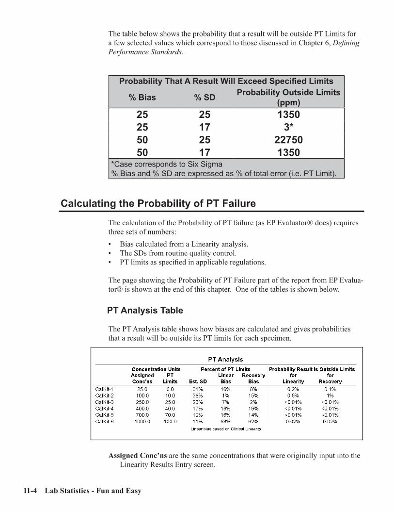
11-4 Lab Statistics - Fun and Easy
The table below shows the probability that a result will be outside PT Limits for a few selected values which correspond to those discussed in Chapter 6, Defining Performance Standards.
Probability That A Result Will Exceed Specified Limits
% Bias % SD Probability Outside Limits (ppm)
25 25 135025 17 3*50 25 2275050 17 1350
*Case corresponds to Six Sigma% Bias and % SD are expressed as % of total error (i.e. PT Limit).
Calculating the Probability of PT Failure
The calculation of the Probability of PT failure (as EP Evaluator® does) requires three sets of numbers:• Bias calculated from a Linearity analysis.• The SDs from routine quality control.• PT limits as specified in applicable regulations. The page showing the Probability of PT Failure part of the report from EP Evalua-tor® is shown at the end of this chapter. One of the tables is shown below.
PT Analysis Table
The PT Analysis table shows how biases are calculated and gives probabilities that a result will be outside its PT limits for each specimen.
Assigned Conc’ns are the same concentrations that were originally input into the Linearity Results Entry screen.
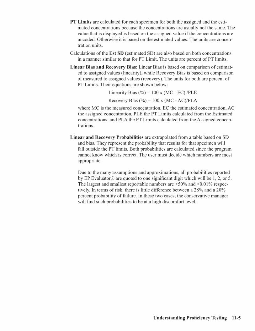
Understanding Proficiency Testing 11-5
PT Limits are calculated for each specimen for both the assigned and the esti-mated concentrations because the concentrations are usually not the same. The value that is displayed is based on the assigned value if the concentrations are uncoded. Otherwise it is based on the estimated values. The units are concen-tration units.
Calculations of the Est SD (estimated SD) are also based on both concentrations in a manner similar to that for PT Limit. The units are percent of PT limits.
Linear Bias and Recovery Bias: Linear Bias is based on comparison of estimat-ed to assigned values (linearity), while Recovery Bias is based on comparison of measured to assigned values (recovery). The units for both are percent of PT Limits. Their equations are shown below:
Linearity Bias (%) = 100 x (MC - EC) /PLERecovery Bias (%) = 100 x (MC - AC)/PLA
where MC is the measured concentration, EC the estimated concentration, AC the assigned concentration, PLE the PT Limits calculated from the Estimated concentrations, and PLA the PT Limits calculated from the Assigned concen-trations.
Linear and Recovery Probabilities are extrapolated from a table based on SD and bias. They represent the probability that results for that specimen will fall outside the PT limits. Both probabilities are calculated since the program cannot know which is correct. The user must decide which numbers are most appropriate.
Due to the many assumptions and approximations, all probabilities reported by EP Evaluator® are quoted to one significant digit which will be 1, 2, or 5. The largest and smallest reportable numbers are >50% and <0.01% respec-tively. In terms of risk, there is little difference between a 28% and a 20% percent probability of failure. In these two cases, the conservative manager will find such probabilities to be at a high discomfort level.
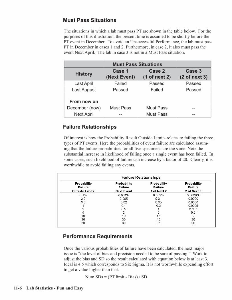
11-6 Lab Statistics - Fun and Easy
Must Pass Situations
The situations in which a lab must pass PT are shown in the table below. For the purposes of this illustration, the present time is assumed to be shortly before the PT event in December. To avoid an Unsuccessful Performance, the lab must pass PT in December in cases 1 and 2. Furthermore, in case 2, it also must pass the event Next April. The lab in case 3 is not in a Must Pass situation.
Must Pass Situations
History Case 1(Next Event)
Case 2(1 of next 2)
Case 3(2 of next 3)
Last April Failed Passed PassedLast August Passed Failed Passed
From now onDecember (now) Must Pass Must Pass --
Next April -- Must Pass --
Failure Relationships
Of interest is how the Probability Result Outside Limits relates to failing the three types of PT events. Here the probabilities of event failure are calculated assum-ing that the failure probabilities for all five specimens are the same. Note the substantial increase in likelihood of failing once a single event has been failed. In some cases, such likelihood of failure can increase by a factor of 20. Clearly, it is worthwhile to avoid failing any events.
Performance Requirements
Once the various probabilities of failure have been calculated, the next major issue is “the level of bias and precision needed to be sure of passing.” Work to adjust the bias and SD so the result calculated with equation below is at least 3. Ideal is 4.5 which corresponds to Six Sigma. It is not worthwhile expending effort to get a value higher than that.
Num SDs = (PT limit - Bias) / SD

Understanding Proficiency Testing 11-7
Statistics
Even though PT limits are designed so that careful, conscientious labs have a good chance of passing PT, there is no guarantee that they will never fail because proficiency testing is based on probabilities. Although a lab can work to reduce the odds of failure so they are close to zero, it can never reduce them completely to zero. The probability of failing the next event as a function of the probability of a result falling outside the PT limits is shown below. The important message is that once the probability of a result being outside the PT limits drops below 0.2% (which corresponds to PT - bias >= 3), then the probabilities of failure become vanish-ingly small, less than 0.01%.
There are approximately 12,000 hospital and reference laboratories in the United States. With each analyzing at least 60 PT analytes, there are a total of 720,000 opportunities for failing each PT event. If the overall probability of an unsatisfac-tory performance for this entire group is 0.01% (1 chance in 10000), then statisti-cally, one would predict 72 unsatisfactory performances in this group.
Calculating the Odds
The more PT tests a lab has on its menu, the more opportunities there are for problems. An insurance actuary would note the increase in “exposure.” If the worst case is a single test with a 1% probability of failure, the probability of pass-ing is 99%. However if 60 tests each has a 1% probability of failure, the overall probability of passing all the tests is 55%.

11-8 Lab Statistics - Fun and Easy
Since both the program and the table make many assumptions, the equations for calculating probabilities are:
• PP = (1 - FP)Overall PP = PP[1] * PP[2] * PP[3] and so on.Overall FP = 1 - Overall PP
where PP is the probability of passing and FP the probability of failing. PP[1], PP[2], etc. is the probability of passing for various analytes.
For example, suppose a lab has 5 analytes with the probabilities of failure as fol-lows: Sodium (5%), Potassium (0.1%), Glucose (5%), Chloride (1%), and BUN (0.2%). Overall probability of passing would be (after converting from percent to fractions):
PP (sodium) = 1 - 0.05 = 0.95PP (potassium) = 1 - 0.001 = 0.999PP (glucose) = 1 - 0.05 = 0.95PP (chloride) = 1 - 0.01 = 0.99PP (BUN) = 1 - 0.002 = 0.998
Overall PP = 0.95 * 0.999 * 0.95 * 0.99 * 0.998Overall PP = 0.89080 = 89%Overall FP = 100 - 89 = 11%
The calculations can be simplified by omitting failure probabilities less than the 25% of the largest probabilities because their contribution are insignificant. In the example above, if the probabilities for chloride (1%), potassium (0.1%) and BUN (0.2%) were omitted, the overall PP changes from 89.08% to 90.25%, an insignifi-cant change.

Understanding Proficiency Testing 11-9
Strategy to Pass Proficiency Testing
Labs should use the following strategy to maximize their chances of passing PT.
Instrument Quality Assurance• Start this process early to avoid surprises.
For example, a few analytes may have serious problems (PT failure probabili-ties greater than 20%), others have significant problems (probabilities of 5 and 10%), still others have minor problems (probabilities of 0.5% to 2.0%) and the rest have no problems.
• Routinely do calibration verification analyses on all analytes to determine how each is performing.
• Calculate the probabilities of PT failure on a regular basis as part of your overall QA management.
• Start work on those with most serious problems first and work down. First work to get the bias down to 25%. Then start on the SDs. If necessary, get your vendor(s) involved. They are anxious that their customers pass PT.For some analytes such as sodium or calcium, the analytical procedure may need to be changed to drop the probabilities low enough. Some labs routinely assay these specimens in duplicate and then average the results in order to reduce random error sufficiently. Remember that you are required by law to treat PT specimens as you would routine patient specimens.
Shortly before PT Survey Day
• Verify calibration on all vulnerable analytes.• Calculate the probabilities of PT failure. If any analytes are vulnerable, ana-
lyze the data carefully to determine if the problem is real or is an artifact of the calculation.
• If necessary, troubleshoot and fix your instrument.
Keep in mind that in the period when the PT results are due, other labs may be having similar problems and that the vendor’s hot line may be very busy. Consequently, keep your instrument in good condition all the time and avoid last minute repairs.

11-10 Lab Statistics - Fun and Easy
On PT Survey Day
The purpose of this exercise is to pass PT. Failing PT can jeopardize the future of your laboratory. Consequently, you should take all legally available measures to increase your odds of success. • Before PT samples are run, run your usual controls to make sure that your
instrument is “on the money.”• Then carefully prepare and analyze the PT samples as if they were patient
specimens. Remember that you cannot analyze PT samples in duplicate un-less you routinely assay patient samples in duplicate.
• Enter the results on the report form and check the entries. Get someone else to check the entries for errors. It is a shame to go through all that work to get everything working properly and then make a mistake reporting the results.

Understanding Proficiency Testing 11-11
Proficiency Testing Report

11-12 Lab Statistics - Fun and Easy

Precision Experiments 12-1
C h a p t e r
12Precision Experiments
In This ChapterPrecision experiments evaluate random error. We discuss:• Deciding which type of precision experiment to perform.• Simple Precision Experiments.• Complex Precision Experiments.• Interpretation of results from precision experiments.
One decision each lab must make is what type of precision experiment to perform. The two possible types of experiments are listed below:
Simple Precision Experiment: About 20 replicates for 2 or 3 specimens assayed all in one run. Another form in which to run this experiment is as a part of a Linearity Experiment which in EP Evaluator®, Release 9 implements Simple Precision as one component of the method validation process.
Complex Precision Experiment: For 2 or 3 specimens, assay each in dupli-cate in 2 runs per day for 3 to 20 days. The 20 day experiment is used in the CLSI:EP5 protocol.
Which experiment to do?
The simple precision experiment is a “quick and dirty” way to fulfill the letter of the precision requirement Its advantage is that it is easy to do. Its disadvantage is that it only tells you about one element of the precision performance of the instrument, namely within-run precision. It says nothing about the other types of precision (between-run, between-day, and total). If the laboratory cares about the quality of its results, we encourage them to perform the complex precision experi-ment. While it does take a little longer, the additional information is valuable.

12-2 Lab Statistics - Fun and Easy
Simple Precision Experiment
Purpose: To establish or verify within-run precision. It is also is frequently used to calculate the monthly means and SDs for QC results.
This procedure is valid for verifying manufacturer’s claims only if the manu-facturer makes within-run precision claims.
Materials: Obtain at least two or possibly three specimens for the precision study. If two specimens are used, one should be in the lower portion of the reportable range and the other should be in the upper portion.
Experiment: Assay each specimen at least 20 times in the same run.Data Required for the Calculations: You need to know an approximate concen-
tration and the results. You have conducted one simple precision experiment for each concentration of analyte. Concentrations can be entered in the form of “Low” or “20” or “Level 1” in EP Evaluator®. Optionally, TEa and the ran-dom error budget can also be entered. If these are entered, then the observed precision can be checked to see if it meets explicit precision requirements.
Calculations: In EP Evaluator®, the appropriate statistics module is Simple Pre-cision. Enter the data and calculate the results.
Key Items to Check
SD and CV: The most important numbers on the page. They should be compared with the manufacturer’s claims at similar concentrations. Keep in mind that an SD marginally larger than that claimed by the manufacturer may not be significant.
Precision Graph: Look for any significant trends in the data. An example would be all the early points being above the mean followed by a drift downward over the analysis period.
Mean: Significant only if the manufacturer’s mean is appreciably different.95% Confidence Interval: This is the range within which the mean is expected
to occur 95% of the time if this experiment were repeated.2 SD Range: This is the range within which individual results are expected to oc-
cur about 95% of the time in future experiments.Precision Graphic: Displays the observed SD complete with a 95% confidence
interval. If the observed SD exceeds the Random Allowable Error (REa), then it fails. However, if the bottom of the 95% CI is less than REa, the user may legitimately declare the experiment as having passed and override the failure declaration of the program. Keep in mind however that the magnitude of the 95% CI is also dependent on the number of results (N) included. As N increas-es, the 95% CI decreases.

Precision Experiments 12-3
Simple Precision Report (Page 1)

12-4 Lab Statistics - Fun and Easy
Complex Precision Experiment
Purpose: To establish or verify precision.This procedure is valid for verifying manufacturer’s claims only if the manu-facturer makes total and within-run precision claims.
Materials: Obtain at least two or possibly three specimens for the precision study. If two specimens are used, one should be in the lower portion of the reportable range and the other should be in the upper portion.
Experiment: The ideal experiment, the standard CLSI:EP5 experiment (not always practical) is 2 replicates per run, 2 runs per day for at least 20 days. Minimum requirements: if 1 run per day or 1 replicate per run, then there must be at least 5 days. Otherwise, at least 3 days or 6 runs whichever comes last.
Data Required for the Calculations: Approximate concentration, the results, vendor’s claimed within-run and total precision. Also of importance is the critical value (either 0.95 or 0.99).The vendor’s precision statistics are not required for the calculation. They are mandatory when verifying the vendor’s claims.
Calculations: In EP Evaluator®, Release 10, the appropriate statistics module is Complex Precision. Enter the data for each experiment and calculate the results.
Key Items to CheckWithin-run and Total SD and Calc’d Pass/Fail: These items verify the vendor’s
claims. If they pass the claims are verified. Note that the user’s SD does not have to be less than the claimed value. It may be larger and still be acceptable.
Concentration (user’s): The overall mean calculated for all the points.Graph: The data should be evenly distributed above and below the mean value
(SDI=0). No obvious trends over time should be evident.

Precision Experiments 12-5
Complex Precision Report (Page 1)
Copyright 1991-2005 David G. Rhoads Associates, Inc.
Page 1Default Printed: 14 Jun 2005 16:40:48EP Evaluator 7.0.0.99
EP Evaluator GLUCOSEClinical Laboratory -- Kennett Community Hospital Instrument: XYZ
Sample Name: HIGH
EP5 Precision
Accepted by:DateSignature
Precision Plot(Different plotting symbols represent different runs)
Standard Deviation
df % CVUser's
User's Claim Value (95%)Verification
Pass/Fail
Within run 40 1.2 2.8 2.5 2.95 PassBetween run 0.7 1.8Between day 0.6 1.4Total 65 1.5 3.6 3.4 3.88 PassMedical Req 65 1.5 3.6 -- -- --
The calculated value passes if it does not exceed the verification value.
Claim EvaluationUser's Concentration: 244.2 Claim Concentration: --
Supporting DataAnalyst Alice DoeAnalysis Date 12 May 2000 to 31 May 2000Days (total/excl) 20 / 0Runs per Day 2Reps per Run 2Critical Value 95%Reagent AA, Lot ABC 87011Calibrator BB, Lot DEF 4700Units mg/dLVerify Mode Verify Vendor ClaimAllowable Total Error --Random Error Budget --Allowable Rand Error --Comment
Outlier Rejection CriteriaSD 3.5 (calculated)Multiplier 5.5Max differencebetween duplicates 19.25
experimentdf for user's
SDwithin run
SDtotal
10 3.8 4.920 3.5 4.530 3.4 4.340 3.3 4.250 3.3 4.260 3.2 4.170 3.2 4.180 3.2 4.190 3.1 4.0100 3.1 4.0
Upper 95% tolerance limit for 95% of user estimates
This table providesdata for a manufact-urer to include inpublished materialsfor users.
Preliminary estimate of precisionMean 243.2SD 3.5
CV 1.4%N 20
Results:242 246 245 246 243242 238 238 247 239241 240 249 241 250245 246 242 243 240

12-6 Lab Statistics - Fun and Easy
Complex Precision Report (Page 2)
Copyright 1991-2005 David G. Rhoads Associates, Inc.
Page 1Default Printed: 14 Jun 2005 16:40:48EP Evaluator 7.0.0.99
EP Evaluator GLUCOSEClinical Laboratory -- Kennett Community Hospital Instrument: XYZ
Sample Name: HIGH
EP5 Precision
Date Results
12 May 2000 242 246245 246
13 May 2000 243 242238 238
14 May 2000 247 239241 240
15 May 2000 249 241250 245
16 May 2000 246 242243 240
17 May 2000 244 245251 247
18 May 2000 241 246245 247
Date Results
19 May 2000 245 245243 245
20 May 2000 243 239244 245
21 May 2000 244 246247 239
22 May 2000 252 251247 241
23 May 2000 249 248251 246
24 May 2000 242 240251 245
25 May 2000 246 249248 240
Date Results
26 May 2000 247 248245 246
27 May 2000 240 238239 242
28 May 2000 241 244245 248
29 May 2000 244 244237 242
30 May 2000 241 239247 245
31 May 2000 247 240245 242
'X' indicates an excluded run, 'O' indicates an outlier run, and 'S' indicates a day that does not have a full complement of results. In all of these cases, the entire day is excluded from the calculations.
Experimental Results
Understanding Reference Intervals 13-1
C h a p t e r
13Understanding Reference
Intervals
In This ChapterVerification or establishment of a correct reference interval is a CLIA ‘88 require-ment. We discuss:• The definition of a reference interval.• The major issues with respect to establishing or verifying a reference interval.• What experiments can be used to verify a proposed reference interval.• What experiments can be used to adjust or establish a reference interval.• Issues with respect to interpretation of results from verification of reference
interval experiments.
Key Concepts
Medical Decision Point: that value for an analyte which represents the boundary between different therapeutic approaches.
Several concepts related to medical decision points are:Normal range: a range of results between two medical decision points which cor-
respond to the central 95% of results from a healthy patient population. It is important to remember that by definition, 2.5% ((100%-95%)/2) of the results will be above the upper limit of the normal range and a similar percentage will be below the lower limit of the normal range. Several examples of normal ranges are shown below.
Note also another pun that of the word “normal”. There are two relevant defi-nitions of this term in this context: one referring to a healthy population, the second a more statistical one referring to a (hoped-for) Gaussian distribution.

13-2 Lab Statistics - Fun and Easy
Table 13.1Examples of Normal Ranges
Analyte Normal RangeAST 5 - 34 U/L
Calcium 8.6 - 10.5 mg/dL (traditional)8.9 - 10.1 mg/dL (Mayo Clinic and others)
Haptoglobin 25 - 193 mg/dLlower 90% CI: 20-33 mg/dLupper 90% CI: 175-210 mg/dL
Note in the case of Haptoglobin, that both lower and upper limits are shown as a 90% CI. The point of this is that reference intervals, just like other statis-tics, also have some uncertainty.
Reference Interval: A pair of medical decision points which frame the limits of results expected for a given condition. All normal ranges are reference inter-vals. Not all reference intervals are normal ranges.
Therapeutic range: Reference interval applied to therapeutic drugs. Establish-ment of a therapeutic range can be very difficult. One of the major problems is collecting specimens from patients who often-times are very sick. Examples are shown in below.
Examples of Therapeutic RangesAnalyte Therapeutic Range
Digoxin 0.8 to 2.0 ng/mLSalicylate <20 mg/dLTheophylline 10-20 ug/mL
Cutoff value: A medical decision point which is often defined with the use of ROC software. For example, there are two cutoff values for cholesterol of 200 and 240 mg/dL. For some analytes such as drugs of abuse, the cutoff values are established administratively.
Sources of Medical Decision Points
Medical decision points and normal ranges can be obtained from several sources:• Medical literature with documented experiments• Manufacturer’s package insert• Normal range studies• ROC curve studies• Web sitesIf a normal range is obtained from an external source, then it must be verified us-ing your laboratory’s patient population before it is put into use.

Understanding Reference Intervals 13-3
Verifying vs. Establishing vs. Neither
While the experiments involved in verifying vs. establishing a normal range seem to be very similar in nature, two fundamental differences are the number of speci-mens involved and the calculations that are performed. The differences in the calculations will be discussed at a later time.
Minimum number of specimens for Verification: 20Minimum number of specimens for Establishment: CLSI:C28 recommends a
minimum of 120 for their non-parametric approach. Fewer can be used but at a cost of a larger confidence interval around the calculated value.
There are an increasing number of tests for which medical decision points and ref-erence intervals are established by the industry. One might say that these are “cast in stone.” These are discussed in a later section.
Verifying a Normal Range
There are two ways to verify a normal range:• Perform a method comparison experiment (such as Chapter 9, Interpreting
Method Comparison Experiments) in which you show that the two methods are statistically identical and that the proposed reference intervals are statisti-cally the same as the previous ones. If the two methods are statistically identical (See Chapter 9, Interpreting Method Comparison Experiments) by all criteria (Deming slope, Deming intercept and medical decision points) then you make the case that you don’t need to perform an actual VRI experiment. The major problem in this argument is the likelihood that even though the two methods are shown to be statistically identical, there are minor differences between them, sufficiently small that they don’t show up as being statistically significant. Consequently, this transfer process can be done once. After that you must either verify or establish the reference interval.If the two methods are not statistically identical, then you must either verify or establish the reference interval.
• Perform a Verification of Reference Interval experiment.

13-4 Lab Statistics - Fun and Easy
Interpretation of VRI Experiments
A normal range is considered to be verified if 90% of the results are within the proposed normal range. This is a broader tolerance than the usual 95% central interval, so it will allow acceptance of a higher percentage of proposed reference intervals (which are assumed to be correct).Several things need to be kept in mind when reviewing the report:• You are confirming that your results are consistent with the proposed normal
range. It is very easy to confirm an inappropriate normal range, such as one which is too wide or which has minor shifts. Consider, for example, the VRI data distributed with the software. Many ref-erence intervals are consistent with these data. All the proposed ranges in the table below would be acceptable according to the verification rules. Note that the width of the narrowest is 30, the width of the widest is 60. Furthermore, the lower limit ranges from 60 to 79, the upper end from 105 to 130.
Examples of Reference Intervals which Pass for One Set of Results
Lower Limit Upper Limit Outside Limits WidthActual Range 75 115 n/a 40Proposed Range 70 110 4.3% 40Range #1 70 115 0% 45Range #2 60 120 0% 60Range #3 75 105 8.7% 30Range #4 79 130 8.7% 51
Some of the characteristics of these proposed ranges are:• Range #2: Too wide for the data.• Range #3: Both limits represent the narrowest ranges.• Range #4: This range is too wide at the high end.If the RI fails the verification process, you must change it. Changing a proposed RI from a value which has been used for a long time is a BIG DEAL!!! Do not do it lightly. You have no idea how your customers use your data.
While it is a lot of work on your part to establish a good range, there is much more effort, pain and expense on the part of your customers to do inappropriate work-ups because of falsely abnormal results produced in your laboratory. It is even more of a problem if diagnoses are missed because your results falsely indi-cated that the marker disease was not present.
Make sure that you use enough specimens to assure the statistical conclusions that you draw are reasonable. Twenty specimens is enough only to verify the RI. It is far from enough to adjust it.
Changing a proposed RI from a value which has been used for a long time is a BIG DEAL!!!

Understanding Reference Intervals 13-5
Establishing a Normal Range
A reference interval (RI), known more familiarly as a normal range, is that range within which the results of a healthy patient are expected to fall. RIs are estab-lished by assaying a large number of specimens from healthy people. Then the re-sults are ordered by value and the central 95% is used. Effectively what happens is that the bottom 2.5% and the top 2.5% are both chopped off from this ordered list.
At first blush, this seems to be simple to fulfill. However some complicating is-sues quickly arise. These come under the categories of analyte type, pre-analytical issues and approach to the calculation.
Analyte Type• If the analyte is not endogenous (i.e. it is a drug), the user may declare the
reference interval / normal range to be zero to zero. However, there is the ad-ditional problem in establishing the therapeutic range. Usually one relies on literature values and/or package inserts.
• In addition, there are many analytes for which reference intervals are inap-propriate, such as cholesterol, HbA1c and the like. Cutoff values are used for these analytes, not reference intervals. Establishing suitable cutoff values is non-trivial. ROC software can be used for this.
Pre-AnalyticalIssues here relate to the population from which the specimens are taken, the care with which they are processed, and the number of specimens.• Ideally, samples are obtained from a healthy population. Often, this require-
ment is difficult to achieve. Possible alternate specimen sources are discussed below.
• The population used to establish or verify the RI must be the same as the population to which the RI applies. For example, the population used to verify or establish the RI for PSA should be males. It should not be the usual laboratory employee population in which young women predominate.
• The number of specimens is important. At least 20 are needed to verify an RI. At least 120 are needed to establish one. Often many more are needed. The reason is that the decision point is not the center of the data but near the ends. Enough specimens must be obtained so that both ends of the curve are adequately defined.
• RIs can differ dramatically with age, gender and lifestyle. These differences need to be anticipated during the specimen collection process. Two examples: a) Hemoglobin concentrations are quite different for a pediatric population than for an adult population; b) Cholesterol concentrations are much lower for a Japanese population than for an American population.

13-6 Lab Statistics - Fun and Easy
• Specimens need to be obtained and using exactly the same approach used for your routine specimens. If you do not store your routine specimens before analysis, do not store the specimens to be used for your RI analysis.
Calculation Approach• In a great many cases, the distribution of results is not Gaussian. Therefore
the simple (un-transformed) parametric calculation of the reference interval mean +/- 2 SD will not work.
• Many additional issues with respect to RI calculations and interpretation of the results are discussed later.
WARNING:Do not calculate the Normal Range from the mean +/-2 SD unless it is very clear that the distribution really is Gaussian or unless it is clear that this approach is the best of all reasonable alternatives.
Possible Specimen Sources
• The ideal source of specimens is from a population known to be healthy.Problem: Often it is difficult to obtain an adequate number of specimens which adequately reflects the use of a particular analyte.
• Collect specimens at a community health fair.Problem: The specimens are unselected and may include some unhealthy individuals (outliers). The calculations must find a way to remove the influ-ence of outliers.Suggestion: Since each analyte is a marker for a disease, the likelihood that there will be specimens from unhealthy persons is related to the prevalence of the disease in the tested population. This means that while specimens from health fairs are poor sources of results for markers of high prevalence diseases such as glucose and lipo-proteins, they may be relatively good sources of results for markers of low prevalence diseases, such as creatinine and calcium.
• Collect a large number of unselected results from an LIS.Problem: The population of results is “contaminated” with many results from sick individuals, some of whom may be very sick. Consequently, you must find some way to remove outliers or else to minimize their influence.
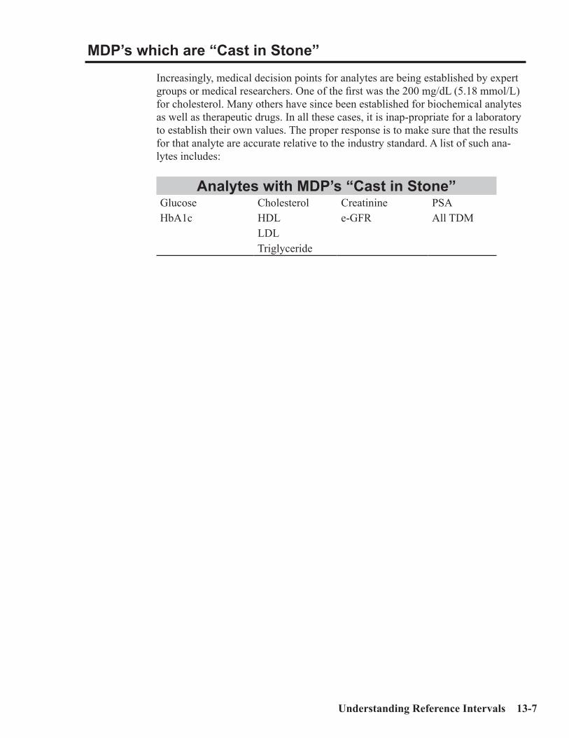
Understanding Reference Intervals 13-7
MDP’s which are “Cast in Stone” Increasingly, medical decision points for analytes are being established by expert groups or medical researchers. One of the first was the 200 mg/dL (5.18 mmol/L) for cholesterol. Many others have since been established for biochemical analytes as well as therapeutic drugs. In all these cases, it is inap-propriate for a laboratory to establish their own values. The proper response is to make sure that the results for that analyte are accurate relative to the industry standard. A list of such ana-lytes includes:
Analytes with MDP’s “Cast in Stone”Glucose Cholesterol Creatinine PSAHbA1c HDL e-GFR All TDM
LDLTriglyceride
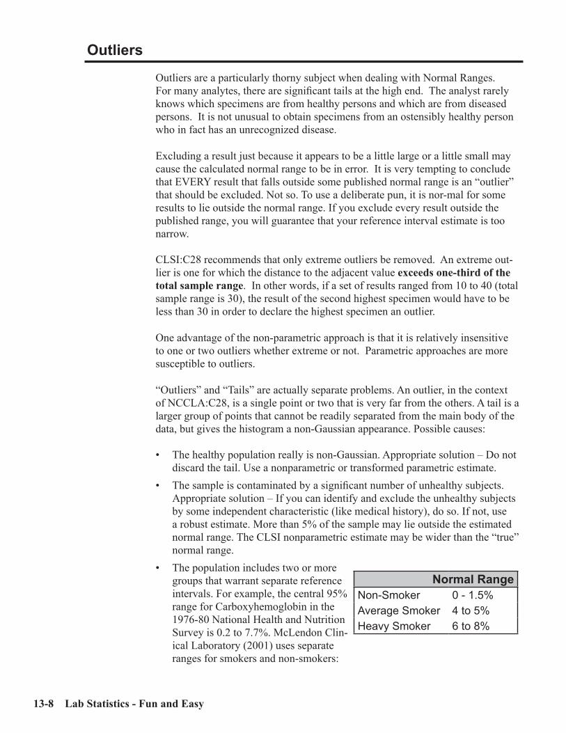
13-8 Lab Statistics - Fun and Easy
Outliers
Outliers are a particularly thorny subject when dealing with Normal Ranges. For many analytes, there are significant tails at the high end. The analyst rarely knows which specimens are from healthy persons and which are from diseased persons. It is not unusual to obtain specimens from an ostensibly healthy person who in fact has an unrecognized disease.
Excluding a result just because it appears to be a little large or a little small may cause the calculated normal range to be in error. It is very tempting to conclude that EVERY result that falls outside some published normal range is an “outlier” that should be excluded. Not so. To use a deliberate pun, it is nor-mal for some results to lie outside the normal range. If you exclude every result outside the published range, you will guarantee that your reference interval estimate is too narrow.
CLSI:C28 recommends that only extreme outliers be removed. An extreme out-lier is one for which the distance to the adjacent value exceeds one-third of the total sample range. In other words, if a set of results ranged from 10 to 40 (total sample range is 30), the result of the second highest specimen would have to be less than 30 in order to declare the highest specimen an outlier.
One advantage of the non-parametric approach is that it is relatively insensitive to one or two outliers whether extreme or not. Parametric approaches are more susceptible to outliers.
“Outliers” and “Tails” are actually separate problems. An outlier, in the context of NCCLA:C28, is a single point or two that is very far from the others. A tail is a larger group of points that cannot be readily separated from the main body of the data, but gives the histogram a non-Gaussian appearance. Possible causes:
• The healthy population really is non-Gaussian. Appropriate solution – Do not discard the tail. Use a nonparametric or transformed parametric estimate.
• The sample is contaminated by a significant number of unhealthy subjects. Appropriate solution – If you can identify and exclude the unhealthy subjects by some independent characteristic (like medical history), do so. If not, use a robust estimate. More than 5% of the sample may lie outside the estimated normal range. The CLSI nonparametric estimate may be wider than the “true” normal range.
• The population includes two or more groups that warrant separate reference intervals. For example, the central 95% range for Carboxyhemoglobin in the 1976-80 National Health and Nutrition Survey is 0.2 to 7.7%. McLendon Clin-ical Laboratory (2001) uses separate ranges for smokers and non-smokers:
Normal RangeNon-Smoker 0 - 1.5%Average Smoker 4 to 5%Heavy Smoker 6 to 8%

Understanding Reference Intervals 13-9
It is very difficult, if not impossible, to distinguish between these situations just by looking at the experimental results.
Accuracy and Precision for Normal Ranges
As part of the process of developing EP Evaluator®, we submitted many differ-ent sets of reference interval data to it. One particularly useful series were sets of patient data (with 1,500 to 20,000 specimens for each analyte) obtained from the NIH. With these data, we were able to develop and test a variety of models to determine which calculation approach would be most effective for the various types of patterns of data.
The way we did this was to make the assumption that the reference interval determined for all the results in a data set was accurate when calculated using CLSI:C28. Then we randomly sampled that data set 50 times for each trial with N ranging from 25 to 1000. We then submitted these various sets of data to our reference interval software and examined the two point estimates and the 90% confidence intervals for both.
We then evaluated the systematic and random error of the various approaches. Systematic error was the difference between the mean estimates of the lower and upper reference interval limits and the correct value. Random error was the dis-persion of the various calculated limits around those computed reference limits. Total error was calculated as the sum of systematic error plus 2 times random error.We observed that:• Random error decreases with increasing N for all approaches. If N increases
by a factor of 4, random error decreases by a factor of 2. Of the algorithms tested, the nonparametric method has the greatest random error.
• While it is somewhat affected by sample size, Systematic Error is more a function of the estimation method (i.e. parametric, nonparametric) than sam-ple size. Error performance of the algorithms is exactly reversed, as compared to random error. The nonparametric method has the least systematic error, and the parametric method has the most.
• If the results have a nice Gaussian distribution, all the approaches work well and give similar results. Both systematic error and random error are low.
• If the results have a significant tail, then there can be substantial amounts of systematic or random error or both regardless of the calculation approach. In a distressingly large number of cases, total error exceeded 20%, sometimes by a large amount, even when N was 120.
• The CLSI non-parametric approach is by far the best approach with large numbers of specimens (N>500) assuming small numbers of outliers (less than 1-2% at either end).
• Transformations can be dangerous with small numbers (<60) of results when outliers are present, since the outliers have undue weight in estimating the transformation. Trying to force a Gaussian distribution to “fit” the outlier makes the reference interval estimate less accurate rather than more accurate.
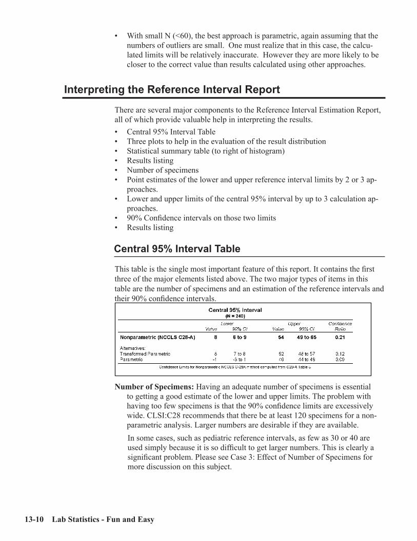
13-10 Lab Statistics - Fun and Easy
• With small N (<60), the best approach is parametric, again assuming that the numbers of outliers are small. One must realize that in this case, the calcu-lated limits will be relatively inaccurate. However they are more likely to be closer to the correct value than results calculated using other approaches.
Interpreting the Reference Interval Report
There are several major components to the Reference Interval Estimation Report, all of which provide valuable help in interpreting the results.• Central 95% Interval Table• Three plots to help in the evaluation of the result distribution• Statistical summary table (to right of histogram)• Results listing• Number of specimens• Point estimates of the lower and upper reference interval limits by 2 or 3 ap-
proaches.• Lower and upper limits of the central 95% interval by up to 3 calculation ap-
proaches.• 90% Confidence intervals on those two limits• Results listing
Central 95% Interval Table
This table is the single most important feature of this report. It contains the first three of the major elements listed above. The two major types of items in this table are the number of specimens and an estimation of the reference intervals and their 90% confidence intervals.
Number of Specimens: Having an adequate number of specimens is essential to getting a good estimate of the lower and upper limits. The problem with having too few specimens is that the 90% confidence limits are excessively wide. CLSI:C28 recommends that there be at least 120 specimens for a non-parametric analysis. Larger numbers are desirable if they are available.In some cases, such as pediatric reference intervals, as few as 30 or 40 are used simply because it is so difficult to get larger numbers. This is clearly a significant problem. Please see Case 3: Effect of Number of Specimens for more discussion on this subject.

Understanding Reference Intervals 13-11
Reference Intervals are calculated by either 2 or 3 approaches. For each ap-proach, a point estimate and a 90% confidence interval are calculated for both the lower and upper limits.
Calculation Approaches
Different types of calculations are used to Establish Reference Intervals in EP Evaluator® because several complicating issues often occur:• Distribution of results in the sample. The fundamental issue here is that in
many cases, the distribution of results is non-Gaussian. In other words the distribution may exhibit skewness and/or kurtosis. In these cases, the conse-quence is that the simple mean/standard deviation calculations, which assume a Gaussian distribution, will not accurately calculate a normal range.
• Difficulty of getting adequate numbers of results. Obtaining the required number of results can be a daunting task in some settings. One of the most difficult is obtaining an adequate number in pediatric settings. It is not easy to obtain 60 specimens from healthy children. Additional complications occur when the RI is age- and gender-related so the number of specimens for a given RI is reduced even further.
• Reducing the effects of tails and outliers. The characteristics of each of these types of calculations is described below:
CLSI:C28 - Non-parametricAdvantages: This is the industry standard. It is relatively simple to use and un-
derstand. One of its best attributes is that it makes no assumptions about the distribution of the data.
Disadvantages: A relatively large number of specimens (minimum of 120) is required.
How it works: The results are ordered by value. With 120 specimens, the lower end of the RI is the value of specimen 3. The upper end is the value of speci-men 118. The 90% confidence interval is defined by the range of several specimens, in this case specimens 1 to 7 at the lower end.
When to use it: Any time you have enough specimens (minimum of 120).
ParametricAdvantages: Easy to understand. Easy to calculate. Often the only reasonable
method for small samples.Disadvantages: Assumes a Gaussian distribution. Sensitive to tails and outliers.
May give a negative lower limit for skewed data.How it works: Simple calculation of mean ± 2 SD.When to use it: Whenever there is a Gaussian distribution of the data, or when
the sample size is very small (N<50) and there are no obvious outliers.

13-12 Lab Statistics - Fun and Easy
Transformed ParametricAdvantages: Conceptual similarities to parametric. Deals effectively with non-
Gaussian distributions. Relatively efficient calculations but not as efficient as the straight parametric approach.
Disadvantages: Relatively difficult to understand and to program. Sensitiveto outliers.How it works: Transforms results to what is hoped to be Gaussian form. Com-
pute mean ±2 SD. Then convert back to original units.When to use it: Whenever the data is transformed into a Gaussian distribution.
RobustIn an early version of EP Evaluator® robust techniques were used. After an ex-tensive study, we removed them because we felt they did not generally improve the calculated RI. While in a few cases there was an improvement, in most cases, there was none. To remove the complexity, we deleted it.
Confidence Interval
The confidence limit indicates the uncertainty of the normal range estimate. In an example shown earlier (Table 13.1), the point estimate for the lower limit of the haptoglobin normal range is 25 mg/dL and the 90% confidence limit is from 20 to 33 mg/dL. It is important to determine the uncertainty in one’s result because then there is a sense of the magnitude of the random error of the estimate of the calculated value.
For example, suppose you calculate the normal range of calcium (traditional range is 8.5 to 10.5 mg/dL) as well as the 90% confidence limits (CI). One’s conclu-sions about the quality of the data are very different if the CI is the relatively tight 8.4 to 8.6 in one case vs. a much looser 8.0 to 9.1 in another.
The major factor affecting the confidence interval is the number of specimens. The CI will tend to halve in size as the number of specimens increases by a factor of four.
A second less important factor is the calculation approach. The un-transformed parametric approach tends to produce the narrowest CI’s. The non-parametric approach tends to produce the widest CI’s. Keep in mind that the parametric ap-proach is susceptible to distribution issues which, under some circumstances, can introduce serious systematic error.
Also, do not assume that the “best” method in the reference interval report is the one with the narrowest CI. The confidence intervals for different methods are not directly comparable. This is particularly true when comparing a parametric meth-od to a non parametric method.
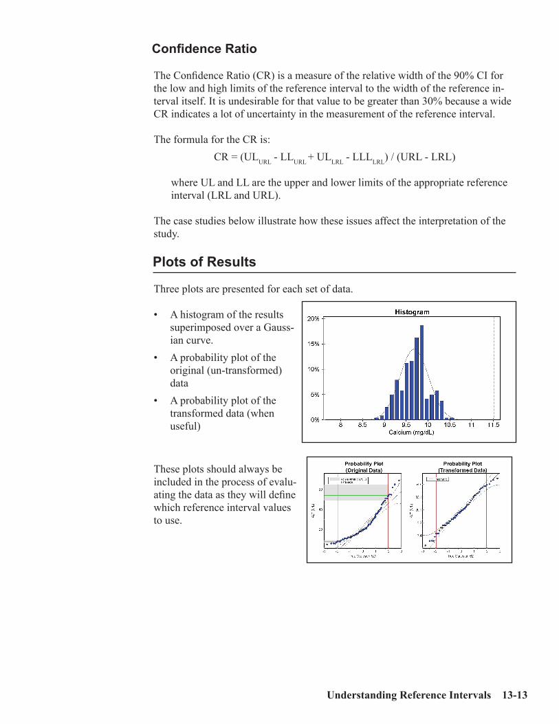
Understanding Reference Intervals 13-13
Confidence Ratio
The Confidence Ratio (CR) is a measure of the relative width of the 90% CI for the low and high limits of the reference interval to the width of the reference in-terval itself. It is undesirable for that value to be greater than 30% because a wide CR indicates a lot of uncertainty in the measurement of the reference interval.
The formula for the CR is: CR = (ULURL - LLURL + ULLRL - LLLLRL) / (URL - LRL)
where UL and LL are the upper and lower limits of the appropriate reference interval (LRL and URL).
The case studies below illustrate how these issues affect the interpretation of the study.
Plots of Results
Three plots are presented for each set of data.
• A histogram of the results superimposed over a Gauss-ian curve.
• A probability plot of the original (un-transformed) data
• A probability plot of the transformed data (when useful)
These plots should always be included in the process of evalu-ating the data as they will define which reference interval values to use.

13-14 Lab Statistics - Fun and Easy
Statistical Analysis Table
This table presents several statistics calculated from the set of results. They include:
Mean and SD
Median
Range of results (lowest and highest results)
N: Number of specimens not excluded and total num-ber of specimens.
Distinct values (the number of unique results)
Central 95% Index. These are the indices of the two values used to establish the lower and upper limits of the non-parametric approach.
Transformation Process
During the calculation process for each set of data, several transforms are automatically attempted. If the transformed data is not significantly better than the un-transformed (original) data, then transformations are not done. Otherwise the best of the transformations is used to calculate the reference interval.
The table of Normalizing Transformations shows the exponent and constant for the transformation process. Non-blank values for the exponent include 0.0 (log), 0.25, 0.5 (square root), 0.75 and 1.00. While it is possible to normalize a wide variety of data sets using a broader range of exponents, this has not been done because it is entirely possible to make absurd data seem good.
Keep in mind that significant errors can be introduced by transforming data sets with small N’s (<60).

Understanding Reference Intervals 13-15
Case 1: An Uncomplicated Example
This is an excellent study with 240 Calcium results obtained from medical stu-dents at the University of Virginia during 1987 and 1988 (Harris and Boyd - 1995). These data are included in the distribution package of EP Evaluator®as the Calcium results in the Default study.
The data has an un-skewed Gaussian distribution. Note that in the triple plots, the histogram shows a more or less even distribution of the data. The data lies nicely on the probability line in the probability plot (original data). Furthermore no transformation was found which significantly improves the fit to a Gaussian distribution. In this case, all the limits are essentially the same. This is expected when the data are Gaussian and there is no transformation.

13-16 Lab Statistics - Fun and Easy
Case 2: Skewed Data
In this study for serum ALT, obtained from the same source as Case 1, the distri-bution of the data is skewed. You can easily tell this by looking at the probability plots. Not only is the data skewed to the left in the histogram, but the data do not lie cleanly on the straight probability line in the Probability Plot with Original data. The data do lie much closer to the probability line in the Transformed Prob-ability Plot.
One major consequence is that the reference interval limits derived from un-trans-formed calculations (parametric and robust - shown in gray) are unreliable. The indicators of this are: a) evidence of skewed data in the triple plots; b) the statis-tics in the Goodness of Fit table indicate skewed data; and c) the lower limit for the parametric approach is a negative number.

Understanding Reference Intervals 13-17
Case 3: Effect of Number of Specimens
Increasing the number of speci-mens has two effects:• The reliability of the estimate of
an RI limit improves.• The size of the 90% CI range
decreases.
The top figure at left shows the estimate and 90% CI of an upper limit of an RI as N varies from 20 to 800. The center line is the estimate, the outer lines the 90% CI limits at each N.
The bottom figure shows how the magnitude of the 90% CI range decreases in size with increasing N. In this case, this range shrinks by a factor of 2 for each four-fold in-crease in the number of specimens. The rate at which the range decreas-es with increasing N also depends on the calculation approach used. It may not decrease at that rate for the non-parametric approaches.

13-18 Lab Statistics - Fun and Easy
Confidence RatioAn important statistic is the confidence ratio (CR).
CR = 0.5*(lower CI range + upper CI range)/(upper RI limit - lower RI limit)
For example with 40 specimens, the CR is about 22% (0.5*2.3/5). With 800 specimens, the CR drops to 5% (0.5*0.5/5), a 4.5-fold improvement. There are two issues in this area:• Making sure that the CR is sufficiently small so that your published RI is
meaningful in the many contexts in which it will be used.• Realizing that while it is desirable to minimize the CI range, the amount of
work involved in getting improved confidence limits will at some point ex-ceed the medical usefulness of the added precision of the measurement. This decision will be closely related to the ease with which you can get additional specimens.
Results for both men and women were included in the calculation. The values shown were calculated from Hgb data using the parametric approach. The data had a Gaussian distribution at all N’s. The first N (ranging from 20 to 800) speci-mens in the set of 905 results obtained from a health fair were used to perform the calculations. This experiment simulates the results as if a laboratory had obtained N specimens from an arbitrary source.
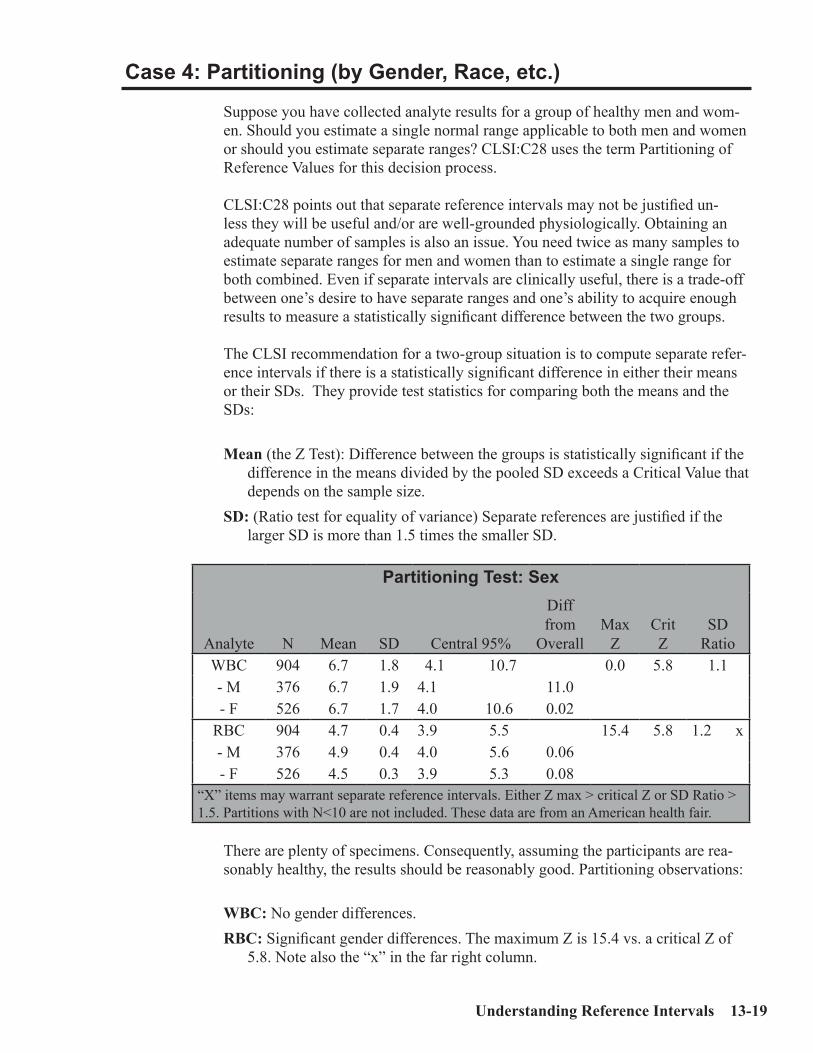
Understanding Reference Intervals 13-19
Case 4: Partitioning (by Gender, Race, etc.)
Suppose you have collected analyte results for a group of healthy men and wom-en. Should you estimate a single normal range applicable to both men and women or should you estimate separate ranges? CLSI:C28 uses the term Partitioning of Reference Values for this decision process.
CLSI:C28 points out that separate reference intervals may not be justified un-less they will be useful and/or are well-grounded physiologically. Obtaining an adequate number of samples is also an issue. You need twice as many samples to estimate separate ranges for men and women than to estimate a single range for both combined. Even if separate intervals are clinically useful, there is a trade-off between one’s desire to have separate ranges and one’s ability to acquire enough results to measure a statistically significant difference between the two groups.
The CLSI recommendation for a two-group situation is to compute separate refer-ence intervals if there is a statistically significant difference in either their means or their SDs. They provide test statistics for comparing both the means and the SDs:
Mean (the Z Test): Difference between the groups is statistically significant if the difference in the means divided by the pooled SD exceeds a Critical Value that depends on the sample size.
SD: (Ratio test for equality of variance) Separate references are justified if the larger SD is more than 1.5 times the smaller SD.
Partitioning Test: Sex
Analyte N Mean SD Central 95%
Diff from
OverallMax
ZCrit Z
SD Ratio
WBC 904 6.7 1.8 4.1 10.7 0.0 5.8 1.1- M 376 6.7 1.9 4.1 11.0- F 526 6.7 1.7 4.0 10.6 0.02
RBC 904 4.7 0.4 3.9 5.5 15.4 5.8 1.2 x- M 376 4.9 0.4 4.0 5.6 0.06- F 526 4.5 0.3 3.9 5.3 0.08
“X” items may warrant separate reference intervals. Either Z max > critical Z or SD Ratio > 1.5. Partitions with N<10 are not included. These data are from an American health fair.
There are plenty of specimens. Consequently, assuming the participants are rea-sonably healthy, the results should be reasonably good. Partitioning observations:
WBC: No gender differences.RBC: Significant gender differences. The maximum Z is 15.4 vs. a critical Z of
5.8. Note also the “x” in the far right column.

13-20 Lab Statistics - Fun and Easy
Case 5: Effect of Outliers
Tails and outliers will always be an issue because data sets which have them no longer have the Gaussian distribution we like to see. The presence of tails and outliers at only one end of the range can easily affect both ends of the RI calcu-lated using the parametric approaches, because they will affect both the mean and SD. Keep in mind that the RI is the central 95% of the healthy population. By definition, 2.5% of the results will be above the upper limit, and a similar number will be below the lower limit. As mentioned previously, outliers and tails are dif-ferent, though related, problems.
Outliers: one or at most two results widely removed from the rest of the data. True outliers may be the inclusion of specimens from one or two sick persons in the study.
Tails occur either because the data really is non-Gaussian or it has results from a mix of multiple populations. There is no clear line of demarcation between the tail and what we want to believe is the “good data.” We will discuss tails further in Case 6.
With respect to outliers, your effort should be to:• Remove the outlier if there is statistical justification.• Remove it if the patient is, in fact, diseased. Base the decision on the patient’s
medical history, NOT on the separation of the suspected outlier from the rest of the population.
• Keep it if you have no independent evidence that the patient is not healthy.
In practice, this is often difficult to do because the person’s medical history is not available to the analyst. For example, if you collect specimens at a health fair or from employee pre-employment physicals, most of the specimens will be from healthy people. Keep in mind that you rarely have assurance that allyour speci-mens are from healthy people. It doesn’t take many specimens to change the answer significantly.
While it is possible to exclude outliers--either subjectively or statistically – based on the magnitude of the result, this is risky. You never know for sure whether an excluded specimen is from a healthy or diseased person. Just because a result is outside a limit, or because it does not fit with your expec-tations for being normal is generally not a satisfactory reason for excluding a result.
CLSI:C28 is very conservative with respect to excluding outliers. It only ex-cludes outliers if the distance between the two most extreme points at one end exceeds one third of the total distance between the lowest and highest points.
With a small sample, a tail in the population may look like an outlier in the sample.

Understanding Reference Intervals 13-21
The data set in this table is for hemoglobin. (N=200) One outlier (value of 9.1 g/dL) was excluded. Notice that except for the upper limit of the non-parametric approach, all the limits increase by about 0.1 g/dL.
Hgb - Central 95% IntervalNo Exclusions w/ Exclustions
Non-parametric 12.4 to 16.7 12.5 to 16.7Parametric 12.23 to 16.90 12.38 to 16.81These data (N=200) were from specimens obtained during a health fair. The data had a Gaussian distribution. One result (Hgb of 9.1 g/dL) was excluded. Three limits (itali-cized and bolded) changed as a result of the exclusion.
By CLSI:C28 standards, there is sufficient justification for excluding this outlier as shown by the calculations below. In this case, the calculated ratio was 0.34. The minimum ratio for excluding a point is 0.33.
Illustration of Outlier DetectionHgb (g/dL)
Smallest Result 9.1Rest of results 11.9 to 17.3Ratio ratio = (11.9-9.1)/(17.3-9.1)
ratio = 2.8/8.2ratio = 0.34
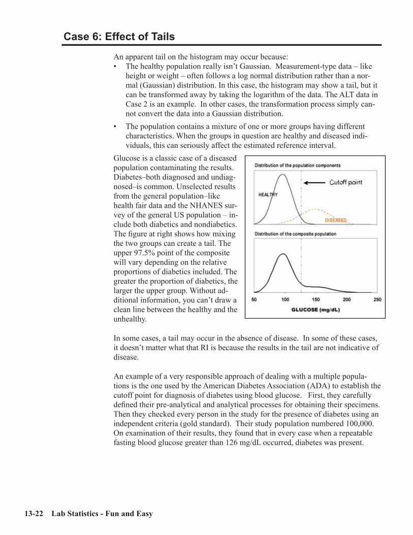
13-22 Lab Statistics - Fun and Easy
Case 6: Effect of Tails
An apparent tail on the histogram may occur because:• The healthy population really isn’t Gaussian. Measurement-type data – like
height or weight – often follows a log normal distribution rather than a nor-mal (Gaussian) distribution. In this case, the histogram may show a tail, but it can be transformed away by taking the logarithm of the data. The ALT data in Case 2 is an example. In other cases, the transformation process simply can-not convert the data into a Gaussian distribution.
• The population contains a mixture of one or more groups having different characteristics. When the groups in question are healthy and diseased indi-viduals, this can seriously affect the estimated reference interval.
Glucose is a classic case of a diseased population contaminating the results. Diabetes–both diagnosed and undiag-nosed–is common. Unselected results from the general population–like health fair data and the NHANES sur-vey of the general US population – in-clude both diabetics and nondiabetics. The figure at right shows how mixing the two groups can create a tail. The upper 97.5% point of the composite will vary depending on the relative proportions of diabetics included. The greater the proportion of diabetics, the larger the upper group. Without ad-ditional information, you can’t draw a clean line between the healthy and the unhealthy.
In some cases, a tail may occur in the absence of disease. In some of these cases, it doesn’t matter what that RI is because the results in the tail are not indicative of disease.
An example of a very responsible approach of dealing with a multiple popula-tions is the one used by the American Diabetes Association (ADA) to establish the cutoff point for diagnosis of diabetes using blood glucose. First, they carefully defined their pre-analytical and analytical processes for obtaining their specimens. Then they checked every person in the study for the presence of diabetes using an independent criteria (gold standard). Their study population numbered 100,000. On examination of their results, they found that in every case when a repeatable fasting blood glucose greater than 126 mg/dL occurred, diabetes was present.

Understanding Reference Intervals 13-23
One strategy which has been used by some investigators (Soldin et al (1999)) is to define an arbitrary cut point. This strategy is used in cases in which the speci-mens are obtained from a mixed population and the investigator is unable to deter-mine whether the individuals are healthy or diseased. The fundamental problem with this approach is that it makes the assumption that the cut point is closely associated with a meaningful and accurate medical decision point.
An example of how this might be done is shown in the experiment below for fasting plasma glucose. While we show this as an example of how this procedure works, we do NOT recommend it. In the data shown in the first set of plots, the data resembles a dog leg (2 relatively straight lines which intersect). Note that in the existing form when all the results are included, the point estimates for the upper reference limits have a poor correlation with the ADA cutoff point. Note that in the existing form when all the results are included, the point estimates for the upper reference limits have a poor correlation with the ADA cutoff point.
If the investigator sets a cut point at approximately 120 mg/dL (the intersection point of the two straight lines), then the data in the lower figure are obtained. Note also that the point estimate now is slightly less than the cut point.
Before Truncating Results
After Truncating Results above 120 mg/dL

13-24 Lab Statistics - Fun and Easy
The table below shows the reference intervals obtained from these data. When you examine these results, keep in mind that the ADA cutoff point is 126 mg/dL. The traditional glucose upper limit is 110 mg/dL.
Upper Reference Limit (mg/dL)Non-
parametric ParametricTransformedParametric
All data 181 151 146After excluding all points above cut point of 120 mg/dL
115 114 114
Data obtained from a health fair. N-904.
I am highly skeptical about the universal validity of reference intervals established after truncation of results, regardless of the truncation approach used. There may be specific cases in which truncation is valid but I will need to see a great deal of evidence before I will endorse the concept.
The point is that you just can’t take any set of patient results and get a valid refer-ence interval. You must think through the specimen acquisition process BEFORE you acquire specimens as that more than anything else will define your eventual reference interval.

Understanding Reference Intervals 13-25
ERI Report showing Effect of Tails (no Truncation)

13-26 Lab Statistics - Fun and Easy
ERI Report showing Effect of Tails (with Truncation)

Sensitivity Experiments 14-1
C h a p t e r
14Sensitivity Experiments
In This ChapterVerification or establishment of sensitivity is a CLIA ‘88 requirement. We discuss:• Several definitions of Sensitivity.• The two types of sensitivity implemented in EP Evaluator® and the situations in
which the use of each is appropriate. • Two experiments to determine Limits of Blank (analytical sensitivity)• Experiment to determine Limits of Quantitation (functional sensitivity)
With the many definitions of Sensitivity in our industry, this subject is potentially very confusing. The three major definitions are:Limits of Blank (LOB): The lowest con-
centration which is statistically signifi-cantly different from zero. Typically, this is defined as the 95% CI around zero. Consequently, some specimens with a concentration of the LOB will in fact have a zero concentration. This type of experiment is suitable for the vast ma-jority of clinical laboratory tests because the low concentrations are not important.
Limits of Detection (LOD): The lowest concentration for which it can be shown that all specimens with a concentration of LOD will be greater than zero. This espe-cially is useful in analysis of drugs of abuse because the analyst wants to be certain that the concentration of drug present in the specimen is greater than zero.
The protocol for performing such an experiment may be found in CLSI:EP17. CLSI:17 is not implemented in EP Evaluator®.
There was a name change between Releases 6 and 7 for EP Evaluator®. The module called Sensi-tivity (Limits of Detection) in Release 6 was renamed Sensitivity (Limits of Blank) in Release 7. The reason for the change was to stay current with the names that CLSI was using for the different types of sensitivity. The calculation process was unchanged.
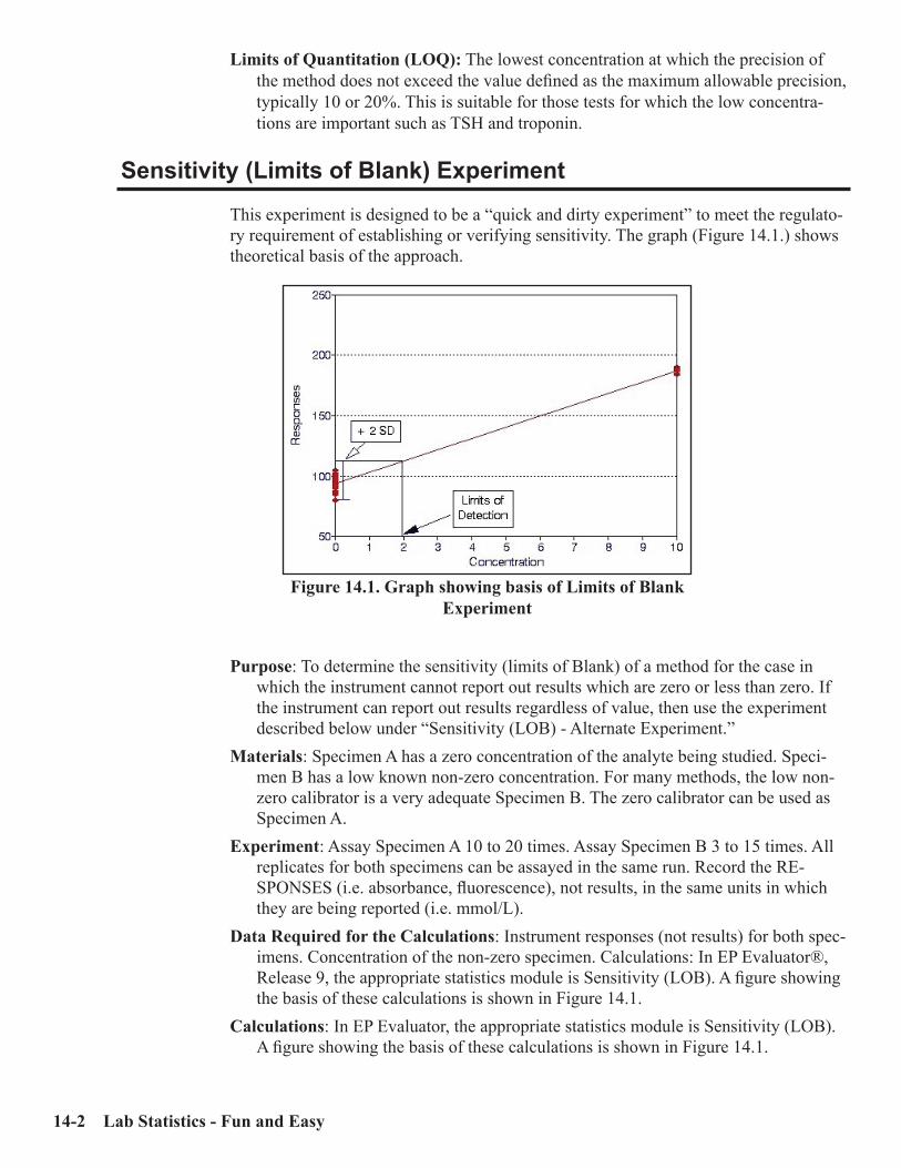
14-2 Lab Statistics - Fun and Easy
Limits of Quantitation (LOQ): The lowest concentration at which the precision of the method does not exceed the value defined as the maximum allowable precision, typically 10 or 20%. This is suitable for those tests for which the low concentra-tions are important such as TSH and troponin.
Sensitivity (Limits of Blank) Experiment
This experiment is designed to be a “quick and dirty experiment” to meet the regulato-ry requirement of establishing or verifying sensitivity. The graph (Figure 14.1.) shows theoretical basis of the approach.
Purpose: To determine the sensitivity (limits of Blank) of a method for the case in which the instrument cannot report out results which are zero or less than zero. If the instrument can report out results regardless of value, then use the experiment described below under “Sensitivity (LOB) - Alternate Experiment.”
Materials: Specimen A has a zero concentration of the analyte being studied. Speci-men B has a low known non-zero concentration. For many methods, the low non-zero calibrator is a very adequate Specimen B. The zero calibrator can be used as Specimen A.
Experiment: Assay Specimen A 10 to 20 times. Assay Specimen B 3 to 15 times. All replicates for both specimens can be assayed in the same run. Record the RE-SPONSES (i.e. absorbance, fluorescence), not results, in the same units in which they are being reported (i.e. mmol/L).
Data Required for the Calculations: Instrument responses (not results) for both spec-imens. Concentration of the non-zero specimen. Calculations: In EP Evaluator®, Release 9, the appropriate statistics module is Sensitivity (LOB). A figure showing the basis of these calculations is shown in Figure 14.1.
Calculations: In EP Evaluator, the appropriate statistics module is Sensitivity (LOB). A figure showing the basis of these calculations is shown in Figure 14.1.
Figure 14.1. Graph showing basis of Limits of Blank Experiment
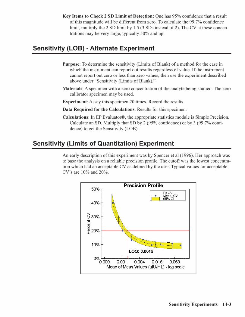
Sensitivity Experiments 14-3
Key Items to Check 2 SD Limit of Detection: One has 95% confidence that a result of this magnitude will be different from zero. To calculate the 99.7% confidence limit, multiply the 2 SD limit by 1.5 (3 SDs instead of 2). The CV at these concen-trations may be very large, typically 50% and up.
Sensitivity (LOB) - Alternate Experiment
Purpose: To determine the sensitivity (Limits of Blank) of a method for the case in which the instrument can report out results regardless of value. If the instrument cannot report out zero or less than zero values, then use the experiment described above under “Sensitivity (Limits of Blank).”
Materials: A specimen with a zero concentration of the analyte being studied. The zero calibrator specimen may be used.
Experiment: Assay this specimen 20 times. Record the results.Data Required for the Calculations: Results for this specimen.Calculations: In EP Evaluator®, the appropriate statistics module is Simple Precision.
Calculate an SD. Multiply that SD by 2 (95% confidence) or by 3 (99.7% confi-dence) to get the Sensitivity (LOB).
Sensitivity (Limits of Quantitation) Experiment
An early description of this experiment was by Spencer et al (1996). Her approach was to base the analysis on a reliable precision profile. The cutoff was the lowest concentra-tion which had an acceptable CV as defined by the user. Typical values for acceptable CV’s are 10% and 20%.

14-4 Lab Statistics - Fun and Easy
Purpose: To determine the sensitivity (Limits of Quantitation) of a method. Experimental Approach: Precision is determined for several specimens over a range
of concentrations. The Limit of Quantitation is the lowest concentration at which the specimen can be quantitated to an acceptable degree of precision, typically with a CV of 10 to 20%. Acceptable precision depends on the analyte.
Materials: A series of specimens with low known concentrations. Their concentrations should increase from one specimen to the next by a factor ranging from 2 to 10. The range of concentrations should be broad enough so that it includes the even-tual cutoff concentration. This range of concentrations may sometimes be obtained from the package insert or a literature search.
Experiment: Assay each specimen at least 10 times, one replicate per day, preferably 20-30 times over a period of several weeks.
Data Required for the Calculations: Results and concentrations for all specimens. Decide in advance what the acceptable CV is for the method.
Calculations: In EP Evaluator®, the appropriate statistics module is Sensitivity (LOD). Enter your data into the program. If your data is wellbehaved, it will deter-mine the cutoff point. This cutoff point corresponds to the concentration at which the upper 95% confidence interval crosses the line corresponding to an acceptable precision.

Published Performance Standards A-1
A p p e n d i x
APublished
Performance StandardsTwo sets of performance standards are listed here. • The first set is the proficiency testing (PT) limits were defined for quantita-
tive assays by the CLIA ‘88 regulations published February 28, 1992. Semi-quantitative or qualitative analytes are not included. In some jurisdictions, other PT limits may apply. Unless otherwise specified, the lower and upper PT limits are obtained by subtracting and adding the specified quantity to the target value.
• The second set are medical requirements as specified by national or govern-mental organizations.
We have provided these lists for your information and convenience. While we have checked them for errors, we do not guarantee that the lists are either com-plete or accurate.
General Immunology
Analyte Name PT LimitAlpha-1 antitrypsin ± 3SDAlpha-fetoprotein (tumor marker) ± 3SDComplement C3 ± 3SDIgA ± 3SDIgB ± 3SD
IgG ± 3SDIgM ± 3SD

A-2 EE User’s Manual
Chemistry
Analyte Name PT LimitAlanine aminotransferase (ALT/SGPT) ± 20%Albumin ± 10%Alkaline phosphatase ± 30%Amylase ± 30%Asparate aminotransferase (AST/SGOT) ± 20%
Bilirubin, total ± 0.4 mg/dL or 20% (greater)Blood gas pO2 ± 3 SDpCO2 ± 5 mm Hg or 8% (greater)pH ± 0.04Calcium, total ± 1.0 mg/dL
Chloride ± 5%Cholesterol, total ± 10%Cholesterol, high density lipoprotein ± 30%Creatine kinase (CPK) ± 30%Creatine kinase isoenzymes MB elevated (presence or absence) or Target value ± 3 SD
Creatinine ± 0.3 mg/dL or 15% (greater)Glucose ± 6 mg/dL or 10% (greater)(excluding glucose performed on monitoring devices cleared by FDA for home use) Iron, total ± 20%Lactate dehyrogenase (LDH) ± 20%LDH isoenzymes LDH1/LDH2 (+ or -) or Target value ±30%
Magnesium ± 25%Potassium ± 0.5 mmol/LSodium ± 4 mmol/LTotal protein ± 10%Triglycerides ± 25%
Urea nitrogen (BUN) ± 2 mg/dL or 9% (greater)Uric acid ± 17%
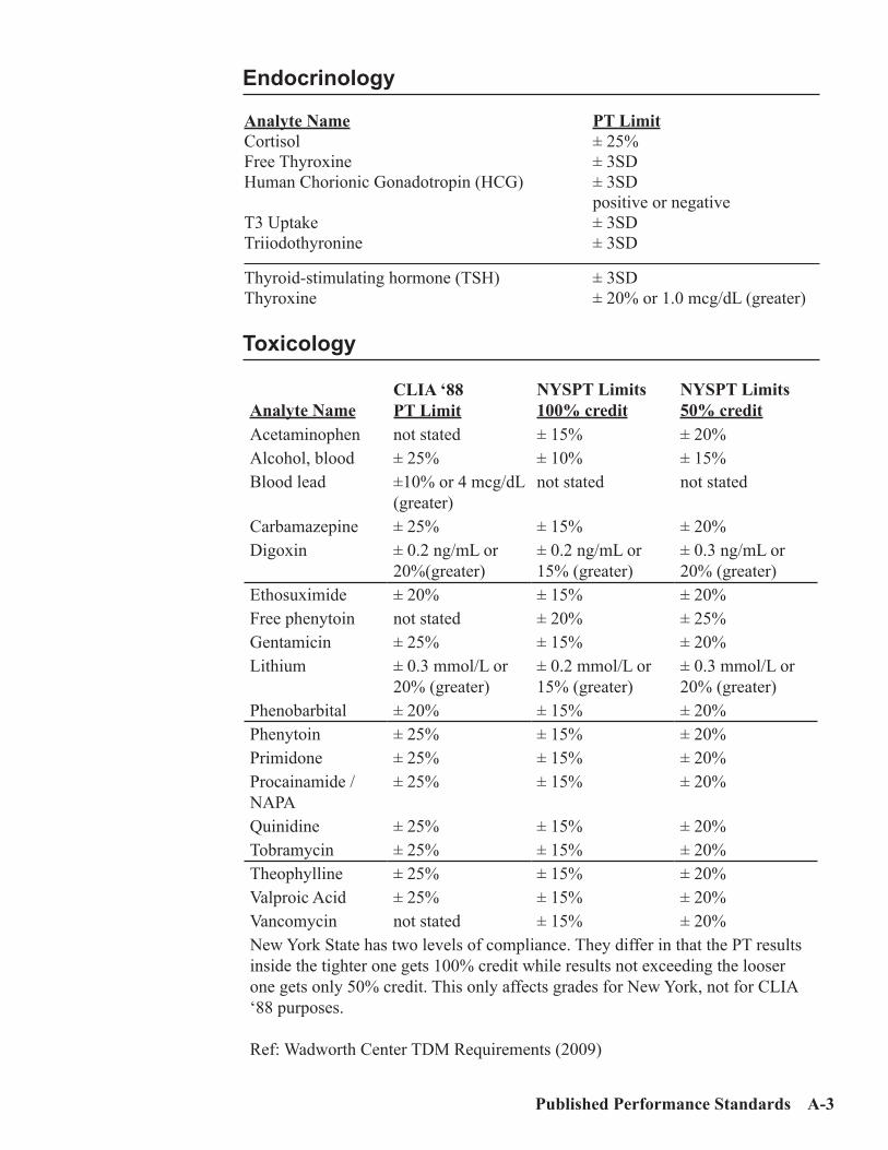
Published Performance Standards A-3
Endocrinology
Analyte Name PT LimitCortisol ± 25%Free Thyroxine ± 3SDHuman Chorionic Gonadotropin (HCG) ± 3SD positive or negativeT3 Uptake ± 3SDTriiodothyronine ± 3SD
Thyroid-stimulating hormone (TSH) ± 3SDThyroxine ± 20% or 1.0 mcg/dL (greater)
Toxicology
Analyte NameCLIA ‘88 PT Limit
NYSPT Limits100% credit
NYSPT Limits50% credit
Acetaminophen not stated ± 15% ± 20%Alcohol, blood ± 25% ± 10% ± 15%Blood lead ±10% or 4 mcg/dL
(greater)not stated not stated
Carbamazepine ± 25% ± 15% ± 20%Digoxin ± 0.2 ng/mL or
20%(greater)± 0.2 ng/mL or 15% (greater)
± 0.3 ng/mL or 20% (greater)
Ethosuximide ± 20% ± 15% ± 20%Free phenytoin not stated ± 20% ± 25%Gentamicin ± 25% ± 15% ± 20%Lithium ± 0.3 mmol/L or
20% (greater)± 0.2 mmol/L or 15% (greater)
± 0.3 mmol/L or 20% (greater)
Phenobarbital ± 20% ± 15% ± 20%Phenytoin ± 25% ± 15% ± 20%Primidone ± 25% ± 15% ± 20%Procainamide / NAPA
± 25% ± 15% ± 20%
Quinidine ± 25% ± 15% ± 20%Tobramycin ± 25% ± 15% ± 20%Theophylline ± 25% ± 15% ± 20%Valproic Acid ± 25% ± 15% ± 20%Vancomycin not stated ± 15% ± 20%New York State has two levels of compliance. They differ in that the PT results inside the tighter one gets 100% credit while results not exceeding the looser one gets only 50% credit. This only affects grades for New York, not for CLIA ‘88 purposes.
Ref: Wadworth Center TDM Requirements (2009)

A-4 EE User’s Manual
Hematology
Analyte Name PT LimitWhite blood cell differential ± 3 SD based on the percentage of dif-
ferent types of white blood cells in the samples.
Erythrocyte count ± 6%Hematocrit (excluding spun hemato-crits)
± 6%
Hemoglobin ± 7%Leukocyte count ± 15%Platelet count ± 25% Fibrinogen ± 20%Partial thromboplastin ± 15%Prothrombin time ± 15%
Medical Requirements
The following values were developed by task groups created by the NIH. In all cases, TEa is defined as bias + 2*CV.
From NCEP (NCEP - 1995).Analyte Name PT LimitCholesterol 9%HDL Cholesterol 13%LDL Cholesterol 12%Triglyceride 15%
From NKEP (Meyers et al - 2006)Analyte Name PT LimitCreatinine 7.6%
From CAP limits as reported by NGSP (2009)Analyte Name PT LimitHbA1c (for 2009B survey) 10% HbA1c (for 2010 surveys) 8%HbA1c (for 2011 surveys and beyond) 7%

Technical CLIS ‘88 Regulations B-1
A p p e n d i x
BTechnical CLIA ‘88 Regulations
from Federal Register, Vol. 68, No. 16Friday, February 24, 2003
42 CFR Pt. 493Rules and Regulations
The following are just those CLIA regulations pertaining to technical issues. The complete CLIA regs can be found at: http://www.phppo.cdc.gov/clia/regs/toc.aspxThe interpretative guidelines and probes may be found at:http://www.cms.hhs.gov/CLIA/downloads/apcsubk1.pdf
Subpart K - Quality Systems for Nonwaived Testing
493.1200 Introduction. (a) Each laboratory that performs nonwaived testing must establish and maintain written policies and procedures that implement and monitor quality systems for all phases of the total testing process (that is, preanalytic, analytic, and postanalytic) as well as general laboratory systems. (b) Each of the laboratory’s quality systems must include an assessment compo-nent that ensures continuous improvement of the laboratory’s performance and services through ongoing monitoring that identifies, evaluates and resolves prob-lems. (c) The various components of the laboratory’s quality systems are used to meet the requirements in this part and must be appropriate for the specialties and subspecialties of testing the laboratory performs, services it offers, and clients it serves.
493.1201 Condition: Bacteriology. (OMITTED)
493.1202 Condition: Mycobacteriology. (OMITTED)
493.1203 Condition: Mycology. (OMITTED)

B-2 Lab Statistics - Fun and Easy
493.1204 Condition: Parasitology. (OMITTED)
493.1205 Condition: Virology. (OMITTED)
493.1207 Condition: Syphilis serology. (OMITTED)
493.1208 Condition: General immunology. If the laboratory provides services in the subspecialty of General immunology, the laboratory must meet the requirements specified in 493.1230 through 493.1256, and 93.1281 through 493.1299.
493.1210 Condition: Routine chemistry. If the laboratory provides services in the subspecialty of Routine chemistry, the laboratory must meet the requirements specified in 493.1230 through 493.1256, 493.1267, and 493.1281 through 493.1299. 493.1211 Condition: Urinalysis. If the laboratory provides services in the subspecialty of Urinalysis, the labora-tory must meet the requirements specified in 493.1230 through 493.1256, and 493.1281 through 493.1299.
493.1212 Condition: Endocrinology. If the laboratory provides services in the subspecialty of Endocrinology, the labo-ratory must meet the requirements specified in 493.1230 through 493.1256, and 493.1281 through 493.1299.
493.1213 Condition: Toxicology. If the laboratory provides services in the subspecialty of Toxicology, the labora-tory must meet the requirements specified in 493.1230 through 493.1256, and 493.1281 through 493.1299.
493.1215 Condition: Hematology. If the laboratory provides services in the specialty of Hematology, the laboratory must meet the requirements specified in 493.1230 through 493.1256, 493.1269, and 493.1281 through 493.1299.
493.1217 Condition: Immunohematology. (OMITTED)
493.1219 Condition: Histopathology. (OMITTED)
493.1220 Condition: Oral pathology. (OMITTED)
493.1221 Condition: Cytology. (OMITTED)
Technical CLIS ‘88 Regulations B-3
493.1225 Condition: Clinical cytogenetics. (OMITTED)
493.1226 Condition: Radiobioassay. (OMITTED)
493.1227 Condition: Histocompatibility. (OMITTED)
493.1230 Condition: General laboratory systems. Each laboratory that performs nonwaived testing must meet the applicable gen-eral laboratory systems requirements in 493.1231 through 493.1236, unless HHS approves a procedure, specified in Appendix C of the State Operations Manual (CMS Pub. 7), that provides equivalent quality testing. The laboratory must moni-tor and evaluate the overall quality of the general laboratory systems and correct identified problems as specified in 493.1239 for each specialty and subspecialty of testing performed.
493.1231 Standard: Confidentiality of patient information. The laboratory must ensure confidentiality of patient information throughout all phases of the total testing process that are under the laboratory’s control.
493.1232 Standard: Specimen identification and integrity. The laboratory must establish and follow written policies and procedures that ensure positive identification and optimum integrity of a patients specimen from the time of collection or receipt of the specimen through completion of testing and reporting of results.
493.1233 Standard: Complaint investigations. The laboratory must have a system in place to ensure that it documents all com-plaints and problems reported to the laboratory. The laboratory must conduct investigations of complaints, when appropriate.
493.1234 Standard: Communications. The laboratory must have a system in place to identify and document problems that occur as a result of a breakdown in communication between the laboratory and an authorized individual who orders or receives test results.
493.1235 Standard: Personnel competency assessment policies. As specified in the personnel requirements in subpart M, the laboratory must establish and follow written policies and procedures to assess employee and, if applicable, consultant competency.

B-4 Lab Statistics - Fun and Easy
493.1236 Standard: Evaluation of proficiency testing perfor-mance. (a) The laboratory must review and evaluate the results obtained on proficiency testing performed as specified in subpart H of this part. (b) The laboratory must verify the accuracy of the following:
(1) Any analyte or subspecialty without analytes listed in subpart I of this part that is not evaluated or scored by a CMS-approved proficiency testing pro-gram.
[Note: The analytes listed in subpart I are the CLIA PT analytes. They are all listed in Appendix A.]
(2) Any analyte, specialty or subspecialty assigned a proficiency testing score that does not reflect laboratory test performance (that is, when the proficiency testing program does not obtain the agreement required for scoring as speci-fied in subpart I of this part, or the laboratory receives a zero score for nonpar-ticipation, or late return of results).
(c) At least twice annually, the laboratory must verify the accuracy of the follow-ing:
(1) Any test or procedure it performs that is not included in subpart I of this part. (2) Any test or procedure listed in subpart I of this part for which compatible proficiency testing samples are not offered by a CMS-approved proficiency testing program.
(d) All proficiency testing evaluation and verification activities must be docu-mented.
493.1239 Standard: General laboratory systems assess-ment. (a) The laboratory must establish and follow written policies and procedures for an ongoing mechanism to monitor, assess, and, when indicated, correct problems identified in the general laboratory system requirements specified at 493.1231 through 493.1236. (b) The general laboratory systems assessment must include a review of the effec-tiveness of corrective actions taken to resolve problems, revision of policies and procedures necessary to prevent recurrence of problems, and discussion of general laboratory systems assessment reviews with appropriate staff. (c) The laboratory must document all general laboratory systems assessment ac-tivities.
Preanalytic Systems
493.1240 Condition: Preanalytic systems. Each laboratory that performs nonwaived testing must meet the applicable preana-lytic system(s) requirements in 493.1241 and 493.1242, unless HHS approves a procedure, specified in Appendix C of the State Operations Manual (CMS Pub. 7),

Technical CLIS ‘88 Regulations B-5
that provides equivalent quality testing. The laboratory must monitor and evaluate the overall quality of the preanalytic systems and correct identified problems as specified in 493.1249 for each specialty and subspecialty of testing performed.
493.1241 Standard: Test request. (a) The laboratory must have a written or electronic request for patient testing from an authorized person. (b) The laboratory may accept oral requests for laboratory tests if it solicits a writ-ten or electronic authorization within 30 days of the oral request and maintains the authorization or documentation of its efforts to obtain the authorization. (c) The laboratory must ensure the test requisition solicits the following informa-tion:
(1) The name and address or other suitable identifiers of the authorized person requesting the test and, if appropriate, the individual responsible for using the test results, or the name and address of the laboratory submitting the speci-men, including, as applicable, a contact person to enable the reporting of im-minently life threatening laboratory results or panic or alert values. (2) The patients name or unique patient identifier. (3) The sex and age or date of birth of the patient. (4) The test(s) to be performed. (5) The source of the specimen, when appropriate. (6) The date and, if appropriate, time of specimen collection. (7) For Pap smears, the patients last menstrual period, and indication of whether the patient had a previous abnormal report, treatment, or biopsy.(8) Any additional information relevant and necessary for a specific test to ensure accurate and timely testing and reporting of results, including interpre-tation, if applicable.
(d) The patients chart or medical record may be used as the test requisition or authorization but must be available to the laboratory at the time of testing and available to CMS or a CMS agent upon request. (e) If the laboratory transcribes or enters test requisition or authorization informa-tion into a record system or a laboratory information system, the laboratory must ensure the information is transcribed or entered accurately.
493.1242 Standard: Specimen submission, handling, and referral. (a) The laboratory must establish and follow written policies and procedures for each of the following, if applicable:
(1) Patient preparation. (2) Specimen collection. (3) Specimen labeling, including patient name or unique patient identifier and, when appropriate, specimen source. (4) Specimen storage and preservation.

B-6 Lab Statistics - Fun and Easy
(5) Conditions for specimen transportation. (6) Specimen processing. (7) Specimen acceptability and rejection. (8) Specimen referral.
(b) The laboratory must document the date and time it receives a specimen. (c) The laboratory must refer a specimen for testing only to a CLIA certified labo-ratory or a laboratory meeting equivalent requirements as determined by CMS. (d) If the laboratory accepts a referral specimen, written instructions must be available to the laboratory’s clients and must include, as appropriate, the informa-tion specified in paragraphs (a)(1) through (a)(7) of this section.
493.1249 Standard: Preanalytic systems assessment. (a) The laboratory must establish and follow written policies and procedures for an ongoing mechanism to monitor, assess, and when indicated, correct problems identified in the preanalytic systems specified at 493.1241 through 493.1242. (b) The preanalytic systems assessment must include a review of the effectiveness of corrective actions taken to resolve problems, revision of policies and proce-dures necessary to prevent recurrence of problems, and discussion of preanalytic systems assessment reviews with appropriate staff. (c) The laboratory must document all preanalytic systems assessment activities. Analytic Systems
493.1250 Condition: Analytic systems. Each laboratory that performs nonwaived testing must meet the applicable analyt-ic systems requirements in 493.1251 through 493.1283, unless HHS approves a procedure, specified in Appendix C of the State Operations Manual (CMS Pub. 7), that provides equivalent quality testing. The laboratory must monitor and evalu-ate the overall quality of the analytic systems and correct identified problems as specified in 493.1289 for each specialty and subspecialty of testing performed.
493.1251 Standard: Procedure manual. (a) A written procedure manual for all tests, assays, and examinations performed by the laboratory must be available to, and followed by, laboratory personnel. Textbooks may supplement but not replace the laboratory’s written procedures for testing or examining specimens. (b) The procedure manual must include the following when applicable to the test procedure:
(1) Requirements for patient preparation; specimen collection, labeling, stor-age, preservation, transportation, processing, and referral; and criteria for specimen acceptability and rejection as described in 493.1242. (2) Microscopic examination, including the detection of inadequately pre-pared slides. (3) Step-by-step performance of the procedure, including test calculations and interpretation of results.

Technical CLIS ‘88 Regulations B-7
(4) Preparation of slides, solutions, calibrators, controls, reagents, stains, and other materials used in testing. (5) Calibration and calibration verification procedures. (6) The reportable range for test results for the test system as established or verified in 493.1253. (7) Control procedures. (8) Corrective action to take when calibration or control results fail to meet the laboratory’s criteria for acceptability. (9) Limitations in the test methodology, including interfering substances. (10) Reference intervals (normal values). (11) Imminently life-threatening test results or panic or alert values. (12) Pertinent literature references. (13) The laboratory’s system for entering results in the patient record and re-porting patient results including, when appropriate, the protocol for reporting imminent life threatening results, or panic, or alert values. (14) Description of the course of action to take if a test system becomes inop-erable.
(c) Manufacturers test system instructions or operator manuals may be used, when applicable, to meet the requirements of paragraphs (b)(1) through (b)(12) of this section. Any of the items under paragraphs (b)(1) through (b)(12) of this section not provided by the manufacturer must be provided by the laboratory. (d) Procedures and changes in procedures must be approved, signed, and dated by the current laboratory director before use. (e) The laboratory must maintain a copy of each procedure with the dates of initial use and discontinuance as described in 493.1105(a)(2).
493.1252 Standard: Test systems, equipment, instruments, reagents, materials, and supplies. (a) Test systems must be selected by the laboratory. The testing must be per-formed following the manufacturer’s instructions and in a manner that provides test results within the laboratory’s stated performance specifications for each test system as determined under 493.1253. (b) The laboratory must define criteria for those conditions that are essential for proper storage of reagents and specimens, accurate and reliable test system opera-tion, and test result reporting. The criteria must be consistent with the manufac-turer’s instructions, if provided. These conditions must be monitored and docu-mented and, if applicable, include the following:
(1) Water quality. (2) Temperature. (3) Humidity. (4) Protection of equipment and instruments from fluctuations and interrup-tions in electrical current that adversely affect patient test results and test
B-8 Lab Statistics - Fun and Easy
reports. (c) Reagents, solutions, culture media, control materials, calibration materials, and other supplies, as appropriate, must be labeled to indicate the following:
(1) Identity and when significant, titer, strength or concentration. (2) Storage requirements. (3) Preparation and expiration dates. (4) Other pertinent information required for proper use. (
(d) Reagents, solutions, culture media, control materials, calibration materials, and other supplies must not be used when they have exceeded their expiration date, have deteriorated, or are of substandard quality. (e) Components of reagent kits of different lot numbers must not be interchanged unless otherwise specified by the manufacturer.
493.1253 Standard: Establishment and verification of per-formance specifications. (a) Applicability. Laboratories are not required to verify or establish performance specifications for any test system used by the laboratory before April 24, 2003. (b)(1) Verification of performance specifications. Each laboratory that introducesan unmodified, FDA-cleared or approved test system must do the following be-fore reporting patient test results:
(i) Demonstrate that it can obtain performance specifications compa-rable to those established by the manufacturer for the following perfor-mance characteristics:
(A) Accuracy.(B) Precision.(C) Reportable range of test results for the test system.
(ii) Verify that the manufacturer’s reference intervals (normal values) are appropriate for the laboratory’s patient population.
(2) Establishment of performance specifications. Each laboratory that modi-fies an FDA-cleared or approved test system, or introduces a test system not subject to FDA clearance or approval (including methods developed in-house and standardized methods such as text book procedures, Gram stain, or potas-sium hydroxide preparations), or uses a test system in which performance specifications are not provided by the manufacturer must, before reporting patient test results, establish for each test system the performance specifica-tions for the following performance characteristics, as applicable:
(i) Accuracy. (ii) Precision. (iii) Analytical sensitivity. (iv) Analytical specificity to include interfering substances. (v) Reportable range of test results for the test system. (vi) Reference intervals (normal values).

Technical CLIS ‘88 Regulations B-9
(vii) Any other performance characteristic required for test perfor-mance.
(3) Determination of calibration and control procedures. The laboratory must determine the test systems calibration procedures and control procedures based upon the performance specifications verified or established under para-graph (b)(1) or (b)(2) of this section.
(c) Documentation. The laboratory must document all activities specified in this section.
493.1254 Standard: Maintenance and function checks. (a) Unmodified manufacturers equipment, instruments, or test systems. The labo-ratory must perform and document the following:
(1) Maintenance as defined by the manufacturer and with at least the frequen-cy specified by the manufacturer. (2) Function checks as defined by the manufacturer and with at least the frequency specified by the manufacturer. Function checks must be within the manufacturers established limits before patient testing is conducted.
(b) Equipment, instruments, or test systems developed in-house, commercially available and modified by the laboratory, or maintenance and function check pro-tocols are not provided by the manufacturer. The laboratory must do the follow-ing:
(1)(i) Establish a maintenance protocol that ensures equipment, instrument, and test system performance that is necessary for accurate and reliable test results and test result reporting.
(ii) Perform and document the maintenance activities specified in para-graph (b)(1)(i) of this section. (2)(i) Define a function check protocol that ensures equipment, instru-ment, and test system performance that is necessary for accurate and reliable test results and test result reporting. (ii) Perform and document the function checks, including background or baseline checks, specified in paragraph (b)(2)(i) of this section. Function checks must be within the laboratory’s established limits be-fore patient testing is conducted.
493.1255 Standard: Calibration and calibration verification procedures. Calibration and calibration verification procedures are required to substantiate the continued accuracy of the test system throughout the laboratory’s reportable range of test results for the test system. Unless otherwise specified in this subpart, for each applicable test system the laboratory must do the following: (a) Perform and document calibration procedures
(1) Following the manufacturers test system instructions, using calibration materials provided or specified, and with at least the frequency recommended by the manufacturer;
B-10 Lab Statistics - Fun and Easy
(2) Using the criteria verified or established by the laboratory as specified in 493.1253(b)(3)
(i) Using calibration materials appropriate for the test system and, if possible, traceable to a reference method or reference material of known value; and (ii) Including the number, type, and concentration of calibration materi-als, as well as acceptable limits for and the frequency of calibration; and
(3) Whenever calibration verification fails to meet the laboratory’s acceptable limits for calibration verification.
(b) Perform and document calibration verification procedures (1) Following the manufacturers calibration verification instructions; (2) Using the criteria verified or established by the laboratory under 493.1253(b)(3)
(i) Including the number, type, and concentration of the materials, as well as acceptable limits for calibration verification; and (ii) Including at least a minimal (or zero) value, a mid-point value, and a maximum value near the upper limit of the range to verify the labora-tory’s reportable range of test results for the test system; and
(3) At least once every 6 months and whenever any of the following occur: (i) A complete change of reagents for a procedure is introduced, unless the laboratory can demonstrate that changing reagent lot numbers does not affect the range used to report patient test results, and control values are not adversely affected by reagent lot number changes. (ii) There is major preventive maintenance or replacement of critical parts that may influence test performance. (iii) Control materials reflect an unusual trend or shift, or are outside of the laboratory’s acceptable limits, and other means of assessing and correcting unacceptable control values fail to identify and correct the problem. (iv) The laboratory’s established schedule for verifying the reportable range for patient test results requires more frequent calibration verifica-tion.
See section at end for Interpretative Guidelines.
493.1256 Standard: Control procedures. (a) For each test system, the laboratory is responsible for having control proce-dures that monitor the accuracy and precision of the complete analytical process. (b) The laboratory must establish the number, type, and frequency of testing control materials using, if applicable, the performance specifications verified or established by the laboratory as specified in 493.1253(b)(3). (c) The control procedures must
(1) Detect immediate errors that occur due to test system failure, adverse envi-
Technical CLIS ‘88 Regulations B-11
ronmental conditions, and operator performance. (2) Monitor over time the accuracy and precision of test performance that may be influenced by changes in test system performance and environmental conditions, and variance in operator performance.
(d) Unless CMS approves a procedure, specified in Appendix C of the State Operations Manual (CMS Pub. 7), that provides equivalent quality testing, the laboratory must
(1) Perform control procedures as defined in this section unless otherwise specified in the additional specialty and subspecialty requirements at 493.1261 through 493.1278. (2) For each test system, perform control procedures using the number and frequency specified by the manufacturer or established by the laboratory when they meet or exceed the requirements in paragraph (d)(3) of this section. (3) At least once each day patient specimens are assayed or examined perform the following for
(i) Each quantitative procedure, include two control materials of differ-ent concentrations; (ii) Each qualitative procedure, include a negative and positive control material; (iii) Test procedures producing graded or titered results, include a negative control material and a control material with graded or titered reactivity, respectively; (iv) Each test system that has an extraction phase, include two control materials, including one that is capable of detecting errors in the extrac-tion process; and (v) Each molecular amplification procedure, include two control mate-rials and, if reaction inhibition is a significant source of false negative results, a control material capable of detecting the inhibition.
(4) For thin layer chromatography (i) Spot each plate or card, as applicable, with a calibrator containing all known substances or drug groups, as appropriate, which are identified by thin layer chromatography and reported by the laboratory; and(ii) Include at least one control material on each plate or card, as ap-plicable, which must be processed through each step of patient testing, including extraction processes.
(5) For each electrophoretic procedure include, concurrent with patient speci-mens, at least one control material containing the substances being identified or measured. (6) Perform control material testing as specified in this paragraph before resuming patient testing when a complete change of reagents is introduced; major preventive maintenance is performed; or any critical part that may in-fluence test performance is replaced. (7) Over time, rotate control material testing among all operators who perform the test.
B-12 Lab Statistics - Fun and Easy
(8) Test control materials in the same manner as patient specimens. (9) When using calibration material as a control material, use calibration ma-terial from a different lot number than that used to establish a cut-off value or to calibrate the test system. (10) Establish or verify the criteria for acceptability of all control materials.
(i) When control materials providing quantitative results are used, sta-tistical parameters (for example, mean and standard deviation) for each batch and lot number of control materials must be defined and avail-able. (ii) The laboratory may use the stated value of a commercially assayed control material provided the stated value is for the methodology and instrumentation employed by the laboratory and is verified by the labo-ratory. (iii) Statistical parameters for unassayed control materials must be established over time by the laboratory through concurrent testing of control materials having previously determined statistical parameters.
(e) For reagent, media, and supply checks, the laboratory must do the following: (1) Check each batch (prepared inhouse), lot number (commercially prepared) and shipment of reagents, disks, stains, antisera, and identification systems (systems using two or more substrates or two or more reagents, or a combina-tion) when prepared or opened for positive and negative reactivity, as well as graded reactivity, if applicable. (2) Each day of use (unless otherwise specified in this subpart), test staining materials for intended reactivity to ensure predictable staining characteristics. Control materials for both positive and negative reactivity must be included, as appropriate. (3) Check fluorescent and immunohistochemical stains for positive and nega-tive reactivity each time of use. (4) Before, or concurrent with the initial use
(i) Check each batch of media for sterility if sterility is required for test-ing; (ii) Check each batch of media for its ability to support growth and, as appropriate, select or inhibit specific organisms or produce a biochemi-cal response; and (iii) Document the physical characteristics of the media when compro-mised and report any deterioration in the media to the manufacturer.
(5) Follow the manufacturers specifications for using reagents, media, and supplies and be responsible for results.
(f) Results of control materials must meet the laboratory’s and, as applicable, the manufacturers test system criteria for acceptability before reporting patient test results. (g) The laboratory must document all control procedures performed.

Technical CLIS ‘88 Regulations B-13
(h) If control materials are not available, the laboratory must have an alternative mechanism to detect immediate errors and monitor test system performance over time. The performance of alternative control procedures must be documented.
493.1261 Standard: Bacteriology. (OMITTED)
493.1262 Standard: Mycobacteriology. (OMITTED)
493.1263 Standard: Mycology. (OMITTED)
493.1264 Standard: Parasitology. (OMITTED)
493.1265 Standard: Virology. (OMITTED)
493.1267 Standard: Routine chemistry.For blood gas analyses, the laboratory must perform the following: (a) Calibrate or verify calibration according to the manufacturers specifications and with at least the frequency recommended by the manufacturer. (b) Test one sample of control material each 8 hours of testing using a combina-tion of control materials that include both low and high values on each day of testing. (c) Test one sample of control material each time specimens are tested unless au-tomated instrumentation internally verifies calibration at least every 30 minutes. (d) Document all control procedures performed, as specified in this section.
493.1269 Standard: Hematology. (a) For manual cell counts performed using a hemocytometer
(1) One control material must be tested each 8 hours of operation; and (2) Patient specimens and control materials must be tested in duplicate.
(b) For all nonmanual coagulation test systems, the laboratory must include two levels of control material each 8 hours of operation and each time a reagent is changed. (c) For manual coagulation tests
(1) Each individual performing tests must test two levels of control materials before testing patient samples and each time a reagent is changed; and(2) Patient specimens and control materials must be tested in duplicate.
(d) The laboratory must document all control procedures performed, as specified in this section.
493.1271 Standard: Immunohematology. (OMITTED)
493.1273 Standard: Histopathology. (OMITTED)

B-14 Lab Statistics - Fun and Easy
493.1274 Standard: Cytology. (OMITTED)
493.1276 Standard: Clinical cytogenetics. (OMITTED)
493.1278 Standard: Histocompatibility. (OMITTED)
493.1281 Standard: Comparison of test results. (a) If a laboratory performs the same test using different methodologies or instru-ments, or performs the same test at multiple testing sites, the laboratory must have a system that twice a year evaluates and defines the relationship between test results using the different methodologies, instruments, or testing sites. (b) The laboratory must have a system to identify and assess patient test results that appear inconsistent with the following relevant criteria, when available:
(1) Patient age. (2) Sex. (3) Diagnosis or pertinent clinical data. (4) Distribution of patient test results. (5) Relationship with other test parameters.
(c) The laboratory must document all test result comparison activities.
493.1282 Standard: Corrective actions. (a) Corrective action policies and procedures must be available and followed as necessary to maintain the laboratory’s operation for testing patient specimens in a manner that ensures accurate and reliable patient test results and reports.(b) The laboratory must document all corrective actions taken, including actions taken when any of the following occur:
(1) Test systems do not meet the laboratory’s verified or established perfor-mance specifications, as determined in 493.1253(b), which include but are not limited to
(i) Equipment or methodologies that perform outside of established operating parameters or performance specifications; (ii) Patient test values that are outside of the laboratory’s reportable range of test results for the test system; and (iii) When the laboratory determines that the reference intervals (nor-mal values) for a test procedure are inappropriate for the laboratory’s patient population.
(2) Results of control or calibration materials, or both, fail to meet the labora-tory’s established criteria for acceptability. All patient test results obtained in the unacceptable test run and since the last acceptable test run must be evalu-ated to determine if patient test results have been adversely affected. The laboratory must take the corrective action necessary to ensure the reporting of accurate and reliable patient test results. (3) The criteria for proper storage of reagents and specimens, as specified
Technical CLIS ‘88 Regulations B-15
under 493.1252(b), are not met. 493.1283 Standard: Test records. (a) The laboratory must maintain an information or record system that includes the following:
(1) The positive identification of the specimen. (2) The date and time of specimen receipt into the laboratory. (3) The condition and disposition of specimens that do not meet the labora-tory’s criteria for specimen acceptability. (4) The records and dates of all specimen testing, including the identity of the personnel who performed the test(s).
(b) Records of patient testing including, if applicable, instrument printouts, must be retained.
493.1289 Standard: Analytic systems assessment. (a) The laboratory must establish and follow written policies and procedures for an ongoing mechanism to monitor, assess, and when indicated, correct problems identified in the analytic systems specified in 493.1251 through 493.1283. (b) The analytic systems assessment must include a review of the effectiveness of corrective actions taken to resolve problems, revision of policies and procedures necessary to prevent recurrence of problems, and discussion of analytic systems assessment reviews with appropriate staff. (c) The laboratory must document all analytic systems assessment activities. Post-analytic Systems.
493.1290 Condition: Postanalytic systems. Each laboratory that performs nonwaived testing must meet the applicable postan-alytic systems requirements in 493.1291 unless HHS approves a procedure, spec-ified in Appendix C of the State Operations Manual (CMS Pub. 7) that provides equivalent quality testing. The laboratory must monitor and evaluate the overall quality of the postanalytic systems and correct identified problems as specified in 493.1299 for each specialty and subspecialty of testing performed.
493.1291 Standard: Test report. (a) The laboratory must have adequate manual or electronic systems in place to ensure test results and other patient specific data are accurately and reliably sent from the point of data entry (whether interfaced or entered manually) to final report destination, in a timely manner. This includes the following:
(1) Results reported from calculated data. (2) Results and patient-specific data electronically reported to network or interfaced systems. (3) Manually transcribed or electronically transmitted results and patient-specific information reported directly or upon receipt from outside referral laboratories, satellite or point-of-care testing locations.

B-16 Lab Statistics - Fun and Easy
(b) Test report information maintained as part of the patients chart or medical re-cord must be readily available to the laboratory and to CMS or a CMS agent upon request. (c) The test report must indicate the following:
(1) For positive patient identification, either the patients name and identifica-tion number, or an unique patient identifier and identification number. (2) The name and address of the laboratory location where the test was per-formed. (3) The test report date. (4) The test performed. (5) Specimen source, when appropriate. (6) The test result and, if applicable, the units of measurement or interpreta-tion, or both. (7) Any information regarding the condition and disposition of specimens that do not meet the laboratory’s criteria for acceptability.
(d) Pertinent reference intervals or normal values, as determined by the laboratory performing the tests, must be available to the authorized person who ordered the tests and, if applicable, the individual responsible for using the test results. (e) The laboratory must, upon request, make available to clients a list of test meth-ods employed by the laboratory and, as applicable, the performance specifications established or verified as specified in 493.1253. In addition, information that may affect the interpretation of test results, for example test interferences, must be provided upon request. Pertinent updates on testing information must be provided to clients whenever changes occur that affect the test results or interpretation of test results. (f) Test results must be released only to authorized persons and, if applicable, the individual responsible for using the test results and the laboratory that initially requested the test. (g) The laboratory must immediately alert the individual or entity requesting the test and, if applicable, the individual responsible for using the test results when any test result indicates an imminent life-threatening condition, or panic or alert values. (h) When the laboratory cannot report patient test results within its established time frames, the laboratory must determine, based on the urgency of the patient test(s) requested, the need to notify the appropriate individual(s) of the delayed testing.
(i) If a laboratory refers patient specimens for testing (1) The referring laboratory must not revise results or information directly related to the interpretation of results provided by the testing laboratory; (2) The referring laboratory may permit each testing laboratory to send the test result directly to the authorized person who initially requested the test. The referring laboratory must retain or be able to produce an exact duplicate of each testing laboratory’s report; and (3) The authorized person who orders a test must be notified by the referring

Technical CLIS ‘88 Regulations B-17
laboratory of the name and address of each laboratory location where the test was performed.
(j) All test reports or records of the information on the test reports must be main-tained by the laboratory in a manner that permits ready identification and timely accessibility.(k) When errors in the reported patient test results are detected, the laboratory must do the following: (1) Promptly notify the authorized person ordering the test and, if applicable, the individual using the test results of reporting errors.
(2) Issue corrected reports promptly to the authorized person ordering the test and, if applicable, the individual using the test results. (3) Maintain duplicates of the original report, as well as the corrected report.
493.1299 Standard: Postanalytic systems assessment. (a) The laboratory must establish and follow written policies and procedures for an ongoing mechanism to monitor, assess and, when indicated, correct problems identified in the postanalytic systems specified in 493.1291. (b) The postanalytic systems assessment must include a review of the effective-ness of corrective actions taken to resolve problems, revision of policies and procedures necessary to prevent recurrence of problems, and discussion of post-analytic systems assessment reviews with appropriate staff. (c) The laboratory must document all postanalytic systems assessment activities.
Selected Interpretative Guidelines
Interpretive Guidelines §493.1255(a) -- CalibrationThe calibration requirement does not apply to a variety of procedures, which include, but are not limited to:• Manual procedures not involving an instrument. . .;• Microscopic procedures . . .; and• Procedures involving an instrument in which calibration is not practical, e.g.,
prothrombin procedures.Laboratories performing testing with instruments that cannot be adjusted (e.g., unit use devices), must follow the manufacturer’s instructions for initial calibra-tion and perform calibration verification as required at §493.1255(b).

B-18 Lab Statistics - Fun and Easy
Interpretive Guidelines §493.1255(b) -- Calibration Verifica-tion
If the laboratory performs a calibration protocol using 3 or more levels of calibra-tion materials that include a low, mid, and high value at least every 6 months, the calibration verification requirement is met.
For kinetic enzymes, the calibration verification requirements may be met by veri-fying the procedure using a high enzyme level material such as a control, calibra-tion material, or patient specimen and diluting it to cover the reportable range.
Control activities routinely used to satisfy the requirement for §493.1256 do not satisfy the calibration verification requirements.
EXCEPTIONS:1 For automated cell counters, the calibration verification requirements are
considered met if the laboratory follows the manufacturer’s instructions for instrument operation and tests 2 levels of control materials each day of testing provided the control results meet the laboratory’s criteria for acceptability.
2 If the laboratory follows the manufacturer’s instruction for instrument opera-tion and routinely tests three levels of control materials (lowest level avail-able, mid-level, and highest level available) more than once each day of test-ing; the control material results meet the laboratory’s criteria for acceptability and the control materials are traceable to National Institute of Standards and Technology (NIST) reference materials, the calibration verification require-ments are met.
Calibration materials, proficiency testing samples with known results, or control materials with known values may be used to perform calibration verification. For these materials, the laboratory must define acceptable limits for the difference be-tween the measured value obtained, versus the actual concen-tration of the materi-als.
If reagents are obtained from a manufacturer and all of the reagents for a test are packaged together, the laboratory is not required to perform calibration verifica-tion for each package of reagents, provided the packages of reagents are received in the same shipment and contain the same lot number.. . .
Probes §493.1255(b)
If a laboratory does not perform calibration verification after a complete change of reagents, what data does the laboratory have to document that changing reagent lot numbers does not affect the reportable range of patient test results, and does not adversely affect control results?
Glossary C-1
A p p e n d i x
CGlossary
Analyte is the substance being measured. Synonyms for analyte are “tests,” “pa-rameters” (hematology) and “measurand.” Examples of analytes are glucose (chemistry), red blood cells (RBC) (hematology), prothrombin time (PT) (hemostasis), phenytoin (toxicology), TSH (endocrinology) and IgG (immu-nology) to mention just a few.
Analyte Concentration is the amount of analyte present in whatever units are be-ing measured, whether an actual concentration (mmol/L), an activity (U/L), time (seconds), cell count percentage or some other measurable quantity.
Assigned Concentrations refers to the concentration of a set of specimens as defined (or assigned) by the user and is used in the assigned concentrations for the linearity and calibration verification protocols. Eleven approaches used in EP Evaluator®, Release 9 to assign concentrations or relative concentrations. For a fuller discussion, refer to the EP Evaluator® User’s Manual Chapter on Linearity.
Bias The difference between two related numbers. There are several definitions of this term. The one frequently used by statisticians is (Ymean - Xmean). A second definition is to indicate the difference between results obtained from two different methods (Yi -Xi). A third is to indicate any difference between two experimental values.
Bias Plot is a graph of the differences between the two results for a single speci-men plotted versus the X result or in the case of the Bland-Altman plot, each difference is plotted versus the average of the X and Y results.
Bins The concept of bins is discussed in Section 3.3 of CLSI:EP9. A suggested list of bins is given in CLSI:EP9 Table I. Bins represent clinical or statistical groups into which results for a given analyte can be distributed. For example, CLSI:EP9 suggests that glucose results be divided into five groups, < 50, 51 to 110, 111 to 150, 151 to 250, and > 250 mg/dl. As the results are entered into the program, the percent in each group are counted and displayed on the data entry screen. The purpose of this concept is to encourage the users to accumu-late results from specimens over a fairly wide analytical range.
Bland-Altman Plot See Bias Plot.

C-2 Lab Statistics - Fun and Easy
Carryover occurs if a specimen or reagent used for the assay of one specimen contaminates the mixture used to assay the next specimen. Usually carryover causes the second specimen to have a falsely high value.
Case has to do with whether a name is spelled with “CAPITAL LETTERS LIKE THIS” (upper case), with “little letters like this” (lower case), or with “Both Capital And Little Letters Like This” (mixed case). (In general, you may input data in either upper or lower case. If the program cares about the case, it will make sure that it receives it in the appropriate form.).
Central Tendency is the center point of the data. Examples of central tendencies are means and medians. See Chapter 4, Statistics 101.
Clinical Linearity is an algorithm by which the linearity of a system can be evaluated against user-defined allowable error. See Chapter 10, Interpreting Linearity Experiments, for details.
CLSI is the acronym for Clinical and Laboratory Standards Institute (formerly known as National Committee for Clinical Laboratory Standards) a voluntary organization which defines standards for the clinical laboratory industry.
Coefficient of Variation (CV) is a common measure of Dispersion. It is a form of SD which has been normalized for concentration using the equation below.
CV = (SD / mean) * 100
Concentration a generic term which refers to the amount of analyte present in a specimen. It may be expressed in whatever units are appropriate to that ana-lyte. It may refer to the concentration of a material such as glucose, the activ-ity of an enzyme such as ALT, clotting time for a hemostasis analyte such as APTT, the number of cells such as neutrophils in hematology.
Confidence Interval The range of values in which results from a large fraction of similar future experiments (usually 95 or 99%) are expected to fall.
Cutoff value: A medical decision point often defined with the use of ROC soft-ware. For example, there are two cutoff values for cholesterol of 200 and 240 mg/dL. For some analytes such as drugs of abuse, the cutoff values are estab-lished administratively.
CV. See Coefficient of Variation.Defined Concentrations: See Assigned Concentrations.Degrees of Freedom is a statistical term for a corrected number of variables used
to calculate a number. Generally, a larger number of degrees of Freedom pro-vides more reliable statistics.
Deming Regression is a regression calculation made assuming that error exists in the data plotted on the X axis. See Regular Regression.
Dispersion is the scatter of data around the central tendency. One example of this would be seen in a Levey-Jennings chart in which typically the results are scattered around the mean.
Drift is the net shift in results over time, either up or down. It is an indicator of the instability of the analytical process. In EP10, it is evaluated in each run.
Experiment refers to the process used to evaluate a single analyte by a single method (i.e. instrument). In many instances, experiments are closely related.

Glossary C-3
Flags indicate a specific condition for a single result or set of results. Examples of flags are exclusion (‘X’) and outlier (‘O’) flags.
Instrument: See Method.Kurtosis refers to the relative steepness of a “bell-shaped” curve as well as the
distribution of results in the tails of the curve.Lab Information System is the computer system which obtains and stores the
laboratory results. Also known as an LIS.Limit of Detection is the lowest concentration of an analyte which is significantly
different from zero. See Chapter 14, Sensitivity Experiments for details.Limits of Quantitation is the lowest concentration of an analyte which can be
measured “accurately.” This is one type of Sensitivity. See Chapter 14, Sensi-tivity Experiments for details.
Linearity is a measure of the degree to which the line segments between a series of points approximates a straight line. There are several definitions of linearity presently used in the clinical laboratory. See Chapter 10, Interpreting Linear-ity Experiments for details.
Linear Regression is a statistical technique which draws a straight line through a population of pairs of data so that it best describes the relationship between the two subsets of data. For a linearity experiment, the two subsets of data are the theoretical (or coded) concentrations and the results obtained from one’s instrument.
LIS: See Lab Information System.Matrix Effects is the term for the case in which significantly different results
are obtained by two different methods. One classic example occurs with the VITROS thin film chemistries when compared with the more conventional wet chemistries. A typical linearity specimen for one test might give a result of 150 units by the first method vs. a result of 285 for the second. Such differenc-es are normally not seen with fresh serum. The differences occur with linearity materials because they are a highly artificial mixture designed for long-term stability and contain specific concentrations of various analytes.
Mean Bias refers to the mean difference between the concentration of an analyte as determined by one method and that determined by another. This term is in the category of Central Tendencies. The related dispersion term is Standard Deviation of the Differences. See that entry for more discussion.
Median is a form of central tendency, namely an estimate of the representative value for a series of numbers. It is calculated by ordering the numbers from low to high. The median is that value such that there are an equal count of numbers above and below it. If N is 5 (an odd number), the median will be the value of the middle number (in this case, the third) . If N is 6 (an even num-ber), the median will be the average of the two middle numbers, in this case numbers 3 and 4.
Medical Decision Point is that value for an analyte which represents the bound-ary between different therapeutic approaches.
C-4 Lab Statistics - Fun and Easy
Method refers to the process which makes measurements on a specimen. Ex-amples of methods include a chemistry instrument which determines glucose concentrations, a hematology analyzer which measures hematocrits, a RIA kit which measures estradiol, a manual microscopic process which counts yeast cells in urine and device which measures pH, pO2 and pCO2. Synonym: Instrument.
Method Comparison is a process which statistically compares two methods. The usual purpose of the comparison process is to show the statistical relationship of the methods being compared. The comparison may be either quantitative or qualitative.
NCCLS: See CLSI.Normal range is a range of results between two medical decision points which
corresponds to the central 95% of results from a healthy patient population. It is one form of a reference interval.
Parameter: 1) An item used to describe a property of a analyte such as units, total allowable error, reference interval and the like; 2) A hematology analyte.
Passing-Bablock is a robust approach to calculating the best straight line through a series of points in a method comparison study. See Chapter 9, Interpreting Method Comparison Experiments for a definition.
Performance Standards is a synonym for Allowable Error. The advantage of using this term is that it is intuitively seen as a positive term. In contrast, the term Allowable Error has negative implications. See Total Allowable Error for a discussion of the term.
POC (Point of Care) (also known as Near Patient Testing) refers to tests which are performed near the patient, as compared to the laboratory which is often at some distance.
POL is the acronym for Physician Office Lab. This is a clinical lab serving one or more physician offices and is managed by a physician.
Policy Definitions are the descriptors of the data needed to define an experiment. Policy definitions allow a user to quickly create an exper-iment, enter or cap-ture results and perform calculations. In other words, they are the non-results type data which must be entered for each experiment such as names, units and reference intervals for analytes, panels, and serial communication parameters to mention but a few.
Precision is a measure of the agreement between replicate measurements of the same specimen.
Prevalence is the frequency with which positives occur in a defined population.Predictive Value Positive is the probability that a subject with a positive result
actually has the disease. It includes prevalence.Predictive Value Negative is the probability that a subject with a negative result
actually does not have the disease.Project is a folder containing a group of experiments by one or more of EP
Evaluator®’s statistical modules. Ideally all those experiments are related; for example, the linearity, precision and method comparison experiments used to evaluate a specific new instrument.

Glossary C-5
Proximity Limits are the acceptable limits for the concentration of the specimen used to test the reportable range. If that concentration is within the proxim-ity limits, then the method passes one part of the two part test for meeting the manufacturer’s claim for the reportable range.
PT Limits (Proficiency Testing Limits) are analytical limits specified by regulato-ry bodies for surveys. The PT limit for glucose is 6 mg/dL or 10% whichever is greater. At a target concentration of 50 mg/dL, the PT limits are 44 to 56. At a target concentration of 200 mg/dL, the PT limits are 180 to 220. For a list of the PT limits specified by CLIA ‘88, see Appendix A, Published Performance Standards.
Random Error Budget is that fraction of TEa which is allocated to 1 SD. Rec-ommended range is 16% (6 SD’s per TEa) to 25% (4 SD’s per TEa). See Chapter 5, Understanding Error and Performance Standards for additional details.
Regression Line is the straight line drawn through the results which minimizes the sum of the square of the distances between each point and the line. Think of it as the “best fit” line.
Recovery is the amount of substance present in a sample that can be detected by the analytical system. Usually this term is referred to as percent recovery. A system in which there is 100% recovery is perfectly accurate.
Reference Interval. See Chapter 13, Understanding Reference Intervals.Regular Regression is a regression calculation made assuming that no error
exists in the data plotted on the X axis. This is also termed “Ordinary Linear Regression.” See also Deming Regression.
Residual is usually calculated in a linear regression environment. It refers to the vertical distance between two numbers, one calculated from a best fit line (often a linear regression line) and an experimental result.
Restore is the process of restoring data, which had previously been backed up, to the original disk. See Backup.
Sensitivity: a) The probability that a test will be positive in a population in which everyone has the disease. The ideal sensitivity is 100%. b) The lowest concen-tration that can be reported (Chapter 14, Sensitivity Experiments for details).
Specificity is the probability that a test will be negative in a population in which no one has the disease. The ideal specificity is 100%.
Skew refers to the position of the mode (highest point of the curve) of the bell shaped distribution relative to the mean. If the mode and the mean are signifi-cantly different, the curve is said to be skewed. See Kurtosis.
SMAD (Scaled Median Absolute Deviation) is a value similar to Standard Error of the Estimate (SEE) in that it describes the scatter around best fit line, but developed with particular relevance to the Passing-Bablok approach as it is insensitive to outliers.
Standard Deviation (SD) describes the degree of dispersion of data around a central value or mean. In a set of normally distributed data, the central 2 SD constitutes about 66% of the results. Similarly the central 4 SD constitutes about 95% of the results.

C-6 Lab Statistics - Fun and Easy
Standard Deviation Index (SDI) is a measure of the distance of a point to the mean described in standard deviation units. The equation for SDI is:
SDI = (result - mean) / SDStandard Deviation of the Differences (SDD) comes from comparing the X
value with the Y value in a given pair of values. It represents the statistical difference between the values of X - Y pairs. One helpful analogy is that the SDD is an “envelope” around the bias similar to the “envelope” of the SD around the mean in a Levey-Jennings chart. When using the terms of central tendency and dispersion, SDD is the dispersion component. Bias is the corre-sponding central tendency.
Standard Error of the Estimate Think of this number (SEE) as the “standard deviation” of the differences between the linear regression line and the plotted points. One helpful analogy is that the SEE is an “envelope” around the re-gression line similar to the “envelope” of the SD around the mean in a Levey-Jennings chart.
String is a line of one or more characters, typically used as a name or descriptor. An example of a string is “GLUCOSE.”
Systematic Error Budget is the fraction of TEa that is to be allocated to system-atic error. Recommended range is 25 to 50%. See Chapter 5, Understanding Error and Performance Standards for additional details.
TEa: See Total Allowable Error.Therapeutic Range is a reference interval applied to therapeutic drugs.Total Allowable Error (TEa) has many definitions. One of these is “the amount of
error that can be tolerated without invalidating the medical usefulness of the analytical result” (Carey and Garber - 1989). A more quantitative way to think of it is “This result is expected to be within X% of the true result 99.7% of the time” where X is the performance standard for this analyte. The “99.7%” may be other values such as 95% or 99.9997%. Synonym: Performance Standards. See Chapter 6, Defining Performance Standards for a substantial discussion on this issue.
Unsatisfactory Performance is defined by CLIA ‘88 regulations as that occasion when the grade during a proficiency event for an analyte is less than 80.
Unsuccessful Performance is defined by CLIA ‘88 regulations as that occasion when there have been Unsatisfactory Performances for an analyte in two of the last three consecutive PT events.
Worksheet is the RRE table into which data is entered prior to moving it into one of the EP Evaluator® statistical modules.

Bibliography D-1
A p p e n d i x
DBibliography
Aspen Conference (1976) Proceedings of the 1976 Aspen Conference on Analytic Goals in Clinical Chemistry, College of American Pathologists, Skokie, IL.
Baltimore Sun (2004) http://www.baltimoresun.com/news/local/bal-hospitalt-ests,0,7736886.storygallery?coll=bal-local-headlines. (Also http://www.westgard.com/essay64.htm#hearings). (accessed 22 August 2005).
R.N. Barnett (1968) Medical Significance of Laboratory Results, Am J Clin Pathol, 50, 671.
R.N. Barnett (1977) Analytical Goals in Clinical Chemistry, the Pathologists Viewpoint. In F.R. Elevitch, editor, Proceedings of the 1976 Aspen Conference on Analytic Goals in Clinical Chemistry, College of American Pathologists, Skokie, IL.
Z. Brooks (2001), Performance-Driven Quality Control AACC, AACC Press, Washington, DC.
CAP (1993) CAP Surveys: Set LN3-A. Calibration Verification/Linearity TDM Survey. College of American Pathologists, Skokie, IL.
C.C. Garber and R.N. Carey (2010) Clinical Chemistry: Theory, Analysis Correla-tion, ed: L.A. Kaplan and A.J. Pesce, Mosby, Inc, an affiicate of Elsevier, Inc, St. Louis.
R.N. Carey, C.C. Garber and D.D. Koch (2000) Concepts and Practices in the Evaluation of Laboratory Methods. Workshop #2103, AACC 52nd Annual Meet-ing, San Francisco, CA, July 23,2000.
K. Casteneda-Mendez (1993) Practical Linearity: A Continuous Improvement Application [Poster] CliniChem ‘93, Albany, NY, October, 1993.
D-2 Lab Statistics - Fun and Easy
CLIA Interpretative Guidelines (2003); For sections related to Calibration and Calibration Verification: http://www.cms.hhs.gov/CLIA/downloads/apcsubk1.pdf
CLSI Document C24-A3. Statistical Quality Control for Quantitative Measure-ment Procedures: Principles and Definitions; Approved Guideline - Third Edition. CLSI, 940 West Valley Road, Suite 1400, Wayne, PA 19087-1898 USA, 2006.
CLSI Document C28-A2. How to define and determine reference intervals in the clinical laboratory; Approved guideline-second edition. CLSI, 940 West Valley Road, Suite 1400, Wayne, PA 19087-1898 USA, 2000. (References to this docu-ment will be to CLSI:C28.)
CLSI Document EP5-A. Evaluation of precision performance of quantitative measurement methods; Approved guideline. CLSI, 940 West Valley Road, Suite 1400, Wayne, PA 19087-1898 USA, 1999. (References to this document will be to CLSI:EP5.)
CLSI Document EP6-A. Evaluation of the linearity of quantitative measurement procedures: a statistical approach; Approved guideline. CLSI, 940 West Valley Road, Suite 1400, Wayne, PA 19087-1898 USA, 2003. (References to this docu-ment will be to CLSI:EP6.)
CLSI Document EP7-A. Interference testing in clinical chemistry; Approved guideline. CLSI, 940 West Valley Road, Suite 1400, Wayne, PA 19087-1898 USA, 2002. (References to this document will be to CLSI:EP7.)
CLSI Document EP9-A. Method comparison and bias estimation using patient samples; Approved guideline. CLSI, 940 West Valley Road, Suite 1400, Wayne, PA 19087-1898 USA, 1995. (References to this document will be to CLSI:EP9.)
CLSI Document EP10-A. Preliminary evaluation of clinical chemistry methods; Approved guideline. CLSI, 940 West Valley Road, Suite 1400, Wayne, PA 19087-1898 USA, 1998. (References to this document will be to CLSI:EP10.)
CLSI Document EP12-A. User protocol for evaluation of qualitative test perfor-mance; Approved guideline. CLSI, 940 West Valley Road, Suite 1400, Wayne, PA 19087-1898 USA, 2002. (References to this document will be to CLSI:EP12.)
CLSI Document EP15-A2. User Verification of Performance for Precision and Trueness; Approved Guideline, second edition. CLSI, West Valley Road, Suite 1400, Wayne, PA 19087-1898 USA, 2005. (References to this document will be to CLSI:EP15.) CLSI Document EP17-A. Protocols for Determination of Limits of Detection and Limits of Quantitation: Approved Guideline. CLSI, West Valley Road, Suite 1400, Wayne, PA 19087-1898 USA, 2004. (References to this document will be to CLSI:EP17.)
Bibliography D-3
CLSI Document GP10-A. Assessment of the clinical accuracy of laboratory tests using receiver operating characteristic (ROC) plots; Approved guideline. CLSI, 940 West Valley Road, Suite 1400, Wayne, PA 19087-1898 USA, 1995. (Refer-ences to this document will be to CLSI:GP10.)
P.J. Cornbleet and N. Gochman (1979) Clin Chem, 25, 432, Incorrect Least-Squares Regression Coefficients in Method-Comparison Analysis.
E. Cotlove et al (1970) Biological and analytic components of variation in long-term studies of serum constituents in normal subjects. III. Physiological and medical implications, Clin Chem 16, 1028.
W.E. Elion-Gerritzen (1980) Analytic Precision in Clinical Chemistry and Medi-cal Decisions, Am J of Clin Pathol 73, 183.
Federal Register (1992), February 18, 1992, 42 CFR Part 405 et al. Medicaid and CLIA Programs; Regulations Implementing the Clinical Laboratory Improvement Amendments of 1988 (CLIA); (Part 493, Subparts I, K and P are relevant to this program. These are the original CLIA ‘88 regulations.)
Federal Register (2003), February 24, 2003, 42 CFR Part 493. Medicaid and CLIA Programs; Regulations Implementing the Clinical Laboratory Improvement Amendments of 1988 (CLIA); (Part 493, Subparts I, K and P are relevant to this program. This reference is the last and final set of CLIA ‘88 regulations.)
R. Forsman (1996), Clinical Chemistry, 42, 813 (1996)
R. Forsman (2004), Clinical Lab News, July 2004, p 12
C.G. Fraser (1987) Desirable standards of performance for therapeutic drug moni-toring. Clin Chem 33, 387.
C.G. Fraser (1987a) Goals for TDM: a correction, Clin Chem 33, 387.
C.G. Fraser (2001) Biological Variation: From Principles to Practice. AACC Press, Washington, DC.
R.S. Galen and S.R. Gambino (1975) Beyond Normality: the predictive value and efficiency of medical diagnoses. John Wiley and Sons, New York.
R. Gilbert (1975) Progress and analytic goals in clinical chemistry, Am J Clin Pathol 63, 960.
Eugene K. Harris and James C. Boyd (1995) Statistical Bases of Reference Values in Laboratory Medicine. Marcel Dekker, Inc., New York
McLendon Clinical Laboratory (2001), UNC Hospitals Manual of Pathology and Laboratory Medicine Clinical Services.

D-4 Lab Statistics - Fun and Easy
N. Mielczarek (2004), Mother not killer, state concedes, Tennessean, Nov. 13, 2004, at 1A (accessed 22 Aug 2005)
G. Myers et al (2006) Recommendations for Improving Serum Creatinine Mea-surement: A Report of the Laboratory Working Group of the National Kidney Disease Education Program. Clin Chem 52, 5.
NCEP (1995). National Cholesterol Education Program, Recommendations on Lipoprotein Measurement by the Working Group on Lipoprotein Measurement. (September, 1995) NIH pub: 95-3044
NGSP (2010). National GlycoProtein Standardization Project, Future Changes in CAP GH2 HbA1c Survey Grading, http://www.ngsp.org/news.asp.
National Reference System for Cholesterol, Cholesterol Reference Method Labo-ratory Network. HDL Cholesterol Certification Protocol for Manufacturers. No-vember 2002. (References to this document will be NRSC-2002 HDL).
National Health and Nutrition Survey (1976-1980). National Center for Health Statistics. National Health and Nutrition Examination Survey, 1976-80. Catalog No 5411, Version 2. U.S. Department of Health and Human Services, Public Health Service, Centers for Disease Control.
New York State PT Surveys. Summaries of these results over many years are available at: http://www.wadsworth.org/labcert/clep/PT/ptindex.html
C.S. Norton-Wenzel (2005) Clinical Chemistry, 51, 1085. EP Evaluator®, CD ROM, Release 6.
Plebani and Carrero (1997) Clinical Chemistry, 43, 1348. Mistakes in a stat labo-ratory: types and frequency
D.G. Rhoads and K. Castaneda-Mendez (1994) Implementation of a Procedure to Determine Clinical Linearity [Poster] CliniChem ‘94, Albany, NY, October, 1994.
J.W. Ross (1980) Blood gas internal quality control, Pathologist, 34, 377.
S.J. Soldin, C. Brugnara, J.M. Hicks (1999) Pediatric Reference Ranges, Third Ed., AACC Press, Washington, DC.
D. Tonks (1963) A study of the accuracy and precision in clinical chemistry deter-minations in 170 Canadian laboratories, Clin Chem 9, 217.
D. Tonks (1968) A quality control program for quantitative clinical chemistry estimations, Can J Med Technol 30, 38.
Wadworth Center TDM Requirements (2009). http://www.wadsworth.org/labcert/clep/ProgramGuide/CLRS_Program_Guide_Update_03_05_09.pdf. Page 102.

Bibliography D-5
J.O. Westgard and Hunt, M.R. (1973) Use and Interpretation of Common Statisti-cal Tests in Method-Comparison Studies. Clin Chem 19, 49.
J.O. Westgard (2002), Basic QC Practices, Second Edition, AACC Press, Wash-ington, DC. Westgard website: An excellent free source of information on setting up and main-taining good QC practices. http://westgard.com/.

D-6 Lab Statistics - Fun and Easy

Our Product Line E-1
A p p e n d i x
EOur Product Line
EP Evaluator®, Release 10
EP Evaluator®, Release 10 (EE), a product of Data Innovations, LLC. is the lead-ing method validation software package in the in-vitro diagnostics industry. It provides statistical modules which deal with all the CLIA ‘88 and CAP technical requirements such as accuracy, precision, reference intervals and reportable range. A review of EP Evaluator, Release 6 (Norton-Wenzel - 2005) had the following comment: “In summary, this software provides a comprehensive collection of statistical ap-plications guaranteed to fit the needs of most clinical laboratories. Comprehensive and professional-looking summary reports are the norm for all modules.” The versions that most hospitals and reference labs acquire have either 10 or 33 statistical modules. The 10 module package provides for all the CLIA require-ments. The 33 module package adds more refined approaches for method compar-isons, sensitivity, and reference intervals. In addition, it now has four lab man-agement modules: Cost per Test, Incident Tracking, Inventory Management and Competency Assessment. A list of the EE10 statistical modules is shown below in Table E.1.The program is offered in five major versions to satisfy the needs of different groups of users. These versions are:• CLIA Version - Low end, entry version of program. For those who need the
basic modules only. Ten statistical modules.• Vendor Version - Designed to meet the needs of field service staff for instru-
ment and reagent vendors. Same ten statistical modules as the CLIA version. However, project management and data capture from instruments are includ-ed. Available only under the subscription plan.
• Standard Version - Simplest version with all 33 statistical modules. Suitable for use in most hospitals and reference labs.
• Standard plus Data Capture Version - Similar to Standard Version but also pro-vides for data capture directly from instruments. We recommend this product for vendors who need more than the minimum ten statistical modules.

E-2 Lab Statistics - Fun and Easy
• Professional Version - Similar to the Standard plus Data Capture version except that in addition it provides network security and audit trail features that many GLP labs need. We recommend this product for: a) all networks with 10 or more concurrent users; b) GLP labs such as those which service the phar-maceutical industry.
Data Transfer FeaturesData can be readily transferred in and out EP Evaluator® by many approaches. These include:• Copy and paste from a spreadsheet.• Input data from a CSV file. (Special text file which may be easily read by
spreadsheet programs among others.)• Capture data directly from instruments. This requires a special program to
communicate with the instrument.• Output data for individual experiments into a CSV file which can then be read
by spreadsheet programs.• Extract data directly and quickly from computers which have ODBC, typi-
cally Middleware systems.
Installation OptionsEP Evaluator® can be purchased with a variety of installation options:• Single PC license. • Network for X concurrent users. Software gets installed on the server. Anyone
with access to the server can use it, but no more than X users at a time. Avail-able for 1, 5, 10 or more concurrent users.
• Site license. Software can be installed on as many PC’s as the user wants at a single street address. Available only for hospitals and academic institutions in the 50 United States and Canada.
Purchase PlansTwo general plans are available:• Perpetual Dating. This is the traditional buy once and own it forever plan. The
user gets 60 days of free telephone support, free updates within their release, and no upgrades to future releases. This plan is available only in the 50 United States and Canada.
• Subscriptions. Basically this is a software rental plan. The usual subscription is for a year. At the end of the initial subscription period, the subscription may be renewed at a 10% discount off list price. Support is provided in two major ways: • Unlimited free telephone support.• Automatic free upgrades to the next release.
Our plan for EP Evaluator® is one of progressive enhancement, namely statistical modules are added with every new release. Consequently, we have provided the subscription plan as an easy, economical mechanism for those who want to stay up to date.

Our Product Line E-3
EP Evaluator® Training WorkshopsWe provide workshops to those who would like to learn more about EP Evalua-tor®. We have given public and private workshops throughout the United States as well as in Canada, Europe and Asia. Contact us by phone or email for more details.
EP Evaluator® - WebcastsFree, live, interactive webcasts are given frequently at scheduled times either weekly or monthly on a variety of EP Evaluator® related topics. Advance signup is required. Consult our website (datainnovations.com) for topics, schedule and signup.
EP Evaluator® - OnlineSeveral statistical modules are also available from our website (datainnovations.com). These statistical modules include most of those in the CLIA version plus a module on Stability.
The user accesses the on-line facility on the website using their browser. They then have a data entry screen. After data is entered and submitted to the website, the website does the calculations and immediately returns a ready-to-print report to the user.
Reports are virtually identical in appearance to the reports generated by the desk-top version of EP Evaluator®.
The cost for most modules is about $1 per report. A block of report credits can be purchased using your credit card on-line or from us directly.
Free Trial and Purchase of EP Evaluator®You may download the desktop version of EP Evaluator® from our website (da-tainnovations.com) and install it on your desktop for a free 14-day trial. You will need administrative privileges to install it on your PC. Product information including a brochure and price list are also available on the website.

E-4 Lab Statistics - Fun and Easy
Statistical Modules in EP Evaluator®, Release 10
Module33 ModuleVersions
10 ModuleVersions
Linearity including Accuracy and Reportable RangeLinearity, Accuracy and Calibration Verification Yes YesSimple Accuracy Yes Yes
Precision (2 modules)Simple Precision Yes YesComplex Precision including CLSI EP5 Yes
Method Comparison (7 modules)Alternate (Quantitative w/ linear regression) Yes YesCLSI EP9 YesQualitative with Semi-quantitative MC Yes YesMultiple Instrument Comparison (no Linear Reg’n) YesTwo Instrument Comparison (no Linear Reg’n) Yes YesGlucose POC Instrument Evaluation YesHematology Studies Yes
Sensitivity (2 modules)Limits of Blank (Analytical) Yes YesLimits of Quantitation (Functional) Yes
Reference Interval (3 modules)Establish Reference Intervals (CLSI C20A) YesROC Plots (for establishing Med Dec Pts) YesVerification of Reference Intervals Yes Yes
Laboratory ManagementIncident Tracking (for lab errors, etc.) YesCost per Test YesInventory Management YesCompetency Assessment Yes
CoagManual INR Check Yes YesINR Geometric Mean and VRI YesPT/INR Method Comparison YesFactor Sensitivity Yes
OtherCarryover Yes YesCLSI EP 10 Preliminary Evaluation of Methods YesInterference (CLSI EP7) YesPerformance Standards YesAverage of Normals (to detect shifts in bias) YesSix Sigma Metrics YesHistogram and Descriptive Stats YesStability YesFor more information on these fine products or to inquire about custom software projects, contact us by phone at (802) 264-3470 or by email at [email protected].
Our Product Line E-5
Instrument ManagerTM
Instrument Manager™ (IM) is a powerful middleware application which initially was designed to facilitate communications between instruments and a laboratory information system (LIS). Over the last 20 years, Data Innovations has developed it into a complete laboratory workflow management system, increasing efficien-cies in pre-analytical, analytical, and post-analytical sample processing and non- analytical tasks such as equipment maintenance. Some of its major uses are:• Connectivity for use in Multi-Site, Multi-LIS, and Multi-workstation environ-
ments supported by a library of over 700 drivers to automation, instrumenta-tion, and various types of information systems.
• Rules-based decision processing via graphical interface with drop down menus which allow you to easily develop rules to support serum indices, real-time delta checking, QC integration, eGFR, reflex and anti-reflex testing and more. You define customized results review screens that support graphics, previous results, filtering and color coding using rules logic.
• Rules Packages for Autoverification specific to each laboratory discipline and including documented algorithms, parameter gathering tools, suites of test data, and validation templates. Standardized result verification enables faster, consistent turn-around time and eliminates mundane tasks whichs allows your scarce medical technologist resources to focus on “true” exceptions.
• Data mining that gives you access to critical information for improving analy-sis and operations by capturing data via a rules based data collection module or by query to the ODBC exposed database.
• Vendor, work area, and sample type independent Sample Storage and Retriev-al which simplifies and organizes your sample storage reducing time to find a sample by an average of 60%.
• Scheduling, tracking, and troubleshooting equipment maintenance tasks are quickly and easily accomplished so you can be inspection ready with Mainte-nance Manager.
Services
Installation, training, 24x7x365 support, and consulting all help you maximize your Return on Investment in IM. Four worldwide offices ensure services are available where and when you need us.
IM is FDA 510(k) cleared and Data Innovations (DI) is ISO 13485 certified.
Availability
IM is available directly from DI and from its numerous business partners. For more information, contact DI at (802) 264-3470, [email protected], or through our website at www.datainnovations.com.

E-6 Lab Statistics - Fun and Easy