SPACE PROGRAMS SUMMARY 37-52, VOL. il

J

Copyright © 1968

Jet Propulsion Laboratory

California Institute of Technology

Prepared Under Contract No. NAS 7-100

National Aeronautics & Space Administration

I_II

Preface

f

The Space Programs Summary is a bimonthly publication that presents a review

of engineering and scientific work performed, or managed, by the Jet Propulsion

Laboratory for the National Aeronautics and Space Administration during a two-

month period. Beginning with the 87-47 series, the Space Programs Summary is

composed of four volumes:

Vol. I. Flight Projects (Unclassified)

Vol. II. The Deep Space Network (Unclassified)

Vol. III. Supporting Research and Advanced Development (Unclassified)

Vol. IV. Flight Projects and Supporting Research and Advanced

Development (Confidential)

Approved by:

W. H. Pickering, Director

Jet Propulsion Laboratory

_ JPL SPACE PROGRAMS SUMMARY 37.52, VOL. II Iii

:w

±

PRICEDING_ PAGI_:Bb,_"qi__- ...... .

7

::L

!

Contents

Introduction ........................ 1

A. Description of the DSN .................... 1

B. Description of DSN Systems .................. 3

1. Command System

K. R. CarterandM. L. Yeater ................... 3

Ih Mission Support ....................... 6

A. Introduction ........................ 6

B. Planetary Flight Projects .................... 7

1. Mariner V Extended Mission Operations Support

D. J. Mudgway ....................... 7

III. Advanced Engineering .................... 11

A. Tracking and Navigational Accuracy: Analysis:

DSN Inherent Accuracy Project .................. 11

1. Introduction

T. W. Hamiltonand D. W. Trask .................. 11

2. Deep Space Station Locations and Physical Constants

Solutions of Surveyor Missions

$. K. Wong ........................ 12

3. Correlations Between Major Visible Lunar Features and Systematic

Variations in Radio-Tracking Data Obtained From

Lunar Orbiter III

w. L, Siogrenand P.M. Muller .................. 20

4. Mariner V Differenced Range-Integrated Range Rate ExperimentF. B. Winn ........................ 25

5. An Approximate Solution to the Analytical Partials of the Spacecraft's

Geocentric Range Rate During the Pre-encounter Phase of a

Planetary Mission

w. E.Bollrnan ....................... 34

6. Continuous Estimation of the State of a Distant Spacecraft During

Successive Passes of Data. Part h Single Tracking Station Results

J. F. Jordan ......................... 37

7. A Program for integrating Lifetime Orbits in Multirevoiution Steps

D. BoggsandR. K. Leavitt .................... 44

B. Communications System Research ................ 46

1. Ranging With Sequential Components46R. M. Goldslein ......................

2. Ephemeris-Controlled Oscillator Analysis

K. D. Schreder ....................... 49

JPL SPACE PROGRAMS SUMMARY 37-52, VOL. U

vi

Contents (contd)

C. Tracking and Data Acquisition Elements Research ........... 58

1. Low-Noise Receivers, Microwave Maser Development,Second-Generation Maser

R. C_ Clauss ....................... 58

2. Improved RF Calibration Techniques:Operating Noise Temperature

Calibration of a Low-Noise Receiving SystemC. T. Stefzried ....................... 61

3. Spacecraft CW Signal Power Calibration With MicrowaveNoise Standards

C. T. Stelzried and O. B. Parham .................. 68

4. Mismatch Error Analysis of Radiometric Method forLine Loss Calibrations

T. Y. Otoshl ....................... 68

5. Waveguide Flange Seal LossMeasurementsC. T. Stelzried, D. L. Mullen, and J. C. Chavez .............. 78

6. EfficientAntenna Systems: X-Band Gain Measurements, 210-ft-diam

Antenna SystemD. A. Ba_hker ....................... 78

D. Supporting Researchand Technology ............... 86

1. Primary Reflector Analysis (210-ft-diam Antenna)M. S. Katow ....................... 86

2. Antenna Structure Joint Integrity Study (Phase II)V. Lobb and F. Stolfer ..................... 92

3. Measurement of Wind Torque (210-ft-diam Antenna)H. McGinness ....................... 97

4. Analysis of Venus DSSModifications for Surface Hysteresis

V. [obb, ]. Carlucci, and F. Stoller ................. 99

IV. Development and Implementation ................ 106

A. Space Flight Operations Facility ................. 106

1. CommunicationsProcessor/7044 Redesign SystemTest Series

R. G. Polansky ....................... ] 06

B. Deep Space Instrumentation Facility ................ 111

1. Venus DSS Activities

F. B. Jackson, M. A. Gregg, and A. L. Price ............... 111

2. Monitor System (Phase I) Monitor Criteria DataR.M. Thomas ....................... 112

3. DSIF/Ground Communications Interface AssemblyE. Garcia ........................ ] 14

4. DSIF Station Control and Data Equipment

E. Bann, A. T. Burke, J, K. Woo, and P. C. Harrison ............. 115

JPL SPACE PROGRAMS SUMMARY 37-52, VOL. II

i

=

I, tl I_

Contents (contd)

5. Echo DSS ReconfigurationF. M. Schiffman ...................... 11 6

C. DSN Systems and Projects ................... 119

1. MMTS: Installation and TestingW. C. Frey ........................ 119

2. MMTS: SDA/Receiver-Exciter InterfaceJ. H. Wilcher ...................... 120

3. MMTS: Bit-SyncLoop Lock DetectorJ. W. Layland, N. A. Burow, and A. Voisnys ............... 121

4. MMTS: 10-MHz Quadrature Generator and Phase Switch

R.B. Crow ........................ 124

5. MMTS: Performance of Subcarrier Demodulator

M. H. Brockman ...................... 1 27

6. High-Rate Telemetry Project: Subcarrier Demodulator PerformanceM. H. Brockman ...................... 141

V. Operations and Systems Data Analysis .............. 144

A. Ground Communications Facility Operations ............. 144

1. Flight Project SupportF. E. Bond, Jr ........................ 144

B. DSN Systems Data Analysis .................. 145

1. Computation of the Normal Matrix for Discrete

Multidimensional ApproximationsA. C. Johnson ....................... 1 45

2. An Improved Method for Range Delay CalibrationS. C. Ward and F. Borncamp ................... 148

Vh Technical Facilities ...................... 151

A. Antennas ......................... 151

1. Woomera DSS Antenna Mechanical UpgradeW. Kissane and M. Kron .................... 151

2. Echo DSSAntenna Mechanical UpgradeR. McKee and J. Carlucci .................... 151

B. Buildings ......................... 152

1. SFOF Mariner Mars 1969 Mission Support Area

M. Salem ....................... 152

C. Utilities ......................... 152

1. Goldstone DSCC Communications Switching Center

B. G. Bridges ....................... 152

2. Air-Conditioner for Venus DSS400-kW-Transmitter Antenna

J. Caducci ........................ 154

JPL SPACE PROGRAMS SUMMARY 37-52, VOL. il vii

!

!

Itll

I. Introduction

A. Description of the DSN

The Deep Space Network (DSN), established by theNASA Office of Tracking and Data Acquisition under the

system management and technical direction of JPL, is

responsible for two-way communications with unmanned

spacecraft traveling approximately 10,000 mi from earth

to interplanetary distances. It supports, or has supported,

the following NASA deep space exploration projects:

Ranger, Surveyor, Mariner Venus 1962, Mariner Mars

1964, Mariner Venus 67, and Mariner Mars 1969 (JPL);

Lunar Orbiter (Langley Research Center); Pioneer (Ames

Research Center); and Apollo (Manned Spacecraft Center),

as backup to the Manned Space Flight Network (MSFN).The DSN is distinct from other NASA networks such as the

MSFN, which has primary responsibility for tracking

the manned spacecraft of the Apollo Project, and the

Space Tracking and Data Acquisition Network (STADAN),

which tracks earth-orbiting scientific and communicationssatellites.

The three basic functions performed by the DSN in

support of each flight project are as follows:

(1) Tracking. Accomplished by radio communication

with the spacecraft, tracking provides such metricdata as angles, radial velocity, and range (distance

from the earth to the spacecraft).

(2) Data acquisition. Using the same radio link, the

data acquisition function consists of the recoveryof information from the spacecraft in the form of

telemetry, namely, the engineering measurements

recorded by the spacecraft and the scientific data

obtained by the onboard instruments.

(3) Command. Using the same radio link, the commandfunction involves sending information to the space-

craft to initiate equipment which, for example,

operates propulsion systems for changing the tra-

jectory of the spacecraft, changes data transmission

rate to earth, or reprograms onboard computerswhich determine the sequence of spacecraft engi-

neering events.

The DSN can be characterized as a set of the following

systems: (1) telemetry, (2) tracking, (3) command, (4)

monitoring, (5) simulation, and (6) operations control.

Alternately, it can be considered as being comprised ofthree facilities: the Deep Space Instrumentation Facility

(DSIF), the Ground Communications Facility (GCF),

and the Space Flight Operations Facility (SFOF).

The DSIF is a worldwide set of deep space stations

(DSSs) that provide basic radio communications with

spacecraft. These stations and the deep space communi-

cations complexes (DSCCs) they comprise are as follows:

o

JPL SPACE PROGRAMS SUMMARY 37-52, VOL. II 1

Pioneer, Echo, and Mars DSSs (and Venus DSS, described

later), comprising the Goldstone DSCC in California;

Woomera, Tidbinbilla, and Booroomba l DSSs, compris-

ing the Canberra DSCC in Australia; Johannesburg DSS

in South Africa; and Robledo, Cebreros, and Rio Cofio 1

DSSs, comprising the Madrid DSCC in Spain. The over-

seas stations are normally staffed and operated by

government agencies of the respective countries, with

some assistance from U.S. support personnel.

In addition, the DSIF operates a compatibility test

station at Cape Kennedy, which is used for verifying

flight-spaeecraft/DSN compat!bility prior to launch, anda flight-project/tracking and data system interface lab-

oratory at JPL, which is used during the development of

the spacecraft to assure a design compatible with the

network. A spacecraft guidance and command station on

Ascension Island serves to track the spacecraft in the

latter part of the launch trajectory while the spacecraftis relatively low in altitude.

To enable continuous radio contact with spacecraft,the stations are located approximately 120 deg apart in

longitude; thus, a spacecraft in flight is always within the

field-of-view of at least one station, and for several hours

each day may be seen by two stations. Furthermore,

since most spacecraft on deep space missions travel

within 80 deg of the equatorial plane, the stations arelocated within latitudes of 45 deg north or south of the

equator.

Radio contact with a spacecraft usually begins when

the spacecraft is on the launch vehicle at Cape Kennedy,

and it is maintained throughout the mission. The early

part of the trajectory is covered by selected network

stations of the Air Force Eastern Test Range (AFETR)

and selected stations of the MSFN which are managed

by Goddard Space Flight Center. Normally, two-way

communications are established between the spacecraftand the DSN within 30 min after spacecraft injection

into lunar, interplanetary, or planetary flight. The Cape

Kennedy DSS, having supported the preflight compati-

bility tests, monitors the spacecraft continuously duringthe launch phase until it passes over the local horizon.

The deep space phase begins with acquisition by either

the Johannesburg, Woomera, or Tidbinbilla DSS. These

stations, with large antennas, low-noise phase-lock receiv-

ing systems, and high-power transmitters, provide radio

communications to the end of the flight. By international

_Not yet authorized.

agreement, the radio frequencies assigned for these func-

tions are 2290-2300 MHz for spacecraft-to-earth downlinkdata transmission and 2110-2120 MHz for earth-to-

spacecraft command and uplink data transmission.

To maintain a state-of-the-art capability, research and

advanced development work on new components and sys-

tems has been conducted continuously at JPL since the

establishment of the DSN. To support this W6rl_,

the Goldstone DSCC has a research and development _4facility designated the Venus DSS, at which the feasi-

bility of new equipment and techniques to be introducedinto the operational network is demonstrated. When a "

new piece of equipment or new technique has been

accepted for integration into the network, it is classed

as Goldstone duplicate standard (GSDS), thus standard-

izing the design and operation of identical items through- :out the network.

The GCF, using, in part, facilities of the worldwide

NASA Communications Facility (NASCOM, managed

and directed by the Goddard Space Flight Center), pro-vides voice, high-speed data, and teletype communica-tions between all stations of the network. Communications

between the Goldstone DSCC and the SFOF are pro-

vided by a microwave system leased from common car-

riers. This microwave link has made possible the

transmission, in real time, of video data received atthe Goldstone DSCC to the SFOF and then to commer-

cial TV systems, as was done during the Ranger andSurveyor missions.

=

2

The SFOF, located at JPL, receives data from all of

the tracking stations and processes that information re-

quired by the flight project to conduct flight operations.Voice and data channels are distributed throughout the

faci!itY, and the following equipment and services areprovided: (1) data-processing equipment for the real-time

handling and display of tracking and telemetry data;

(2) real-time and non-real-time telemetry processing;

(8) simulation equipment for flight projects, as well as

for network use in training of personnel; (4) monitoring

equipment for evaluation of network performance in

near-real time; (5) operations control consoles and status

and operational display facilities required for the con-

duct of flight operations; and (6) technical areas for flight

project personnel who analyze spacecraft performance,

trajectories, and generation of commands, as well as

support services required to carry out those functions,

such as internal communications by telephone, intercom,

public address, closed-circuit TV, documentation, and


1|i

reproduction of data packages. The SFOF is equipped to

support many spacecraft in flight and those under test in

preparation for flight; e.g., over a 24-h period during 1967,

as many as eight spacecraft in flight or in operational-

readiness tests for flight were supported by the SFOF.

Thus, the DSN simultaneously conducts research and

development for support of future [light projects, imple-

ments demonstrated capabilities for support of the more

immediate flight projects, and provides direct support for

the currently active missions, while accommodating dif-

ferences in the individual projects. In this and futureissues of the SPS, Vol. II, the current technical activities

of the DSN in these three general categories will be

reported under the following subject areas:

Introduction

Description of the DSN

Description of DSN Systems

Mission SupportIntroduction

Interplanetary Flight ProjectsPlanetary Flight Projects

Manned Space Flight Project

Advanced Engineering

Tracking and Navigational Accuracy Analysis

Communications System Research

Tracking and Data Acquisition Elements Research

Supporting Research and Technology

Development and Implementation

Space Flight Operations Facility

Ground Communications Facility

Deep Space Instrumentation Facility

DSN Systems and Projects

Operations and Systems Data Analysis

SFOF Operations

GCF Operations

DSIF Operations

DSN Systems Operations

DSN Systems Data Analysis

Technical Facilities

Antennas

BuildingsUtilities

In the section entitled "Description of DSN Systems,"

the status of recent developments for each of the sixDSN systems listed above will be described. The more

fundamental research carried out in support of the DSN

is reported in Vol. III of the SPS, and ]PL flight project

activities for missions supported by the DSN are reportedin Vol. I.

B. Description of DSN Systems

1. Command System, _. R.CarferandM. L.Yeater

a. Functions. The DSN command system provjdes a

medium for command generation, transmission to the

spacecraft, and verification at appropriate points, as well

as for generation of a command master data record

(MDR). The commands are generated in the SFOF,

transferred to the DSIF by means of the GCF, and trans-

mitted to the spacecraft after handling by the mission-

dependent equipment (MDE) at a DSS.

b. System elements. No standard DSN command

system configuration exists at the present time. Each

flight project uses a different system configuration, and

different sets of procedures, MDE at the DSS, and

mission-dependent software in the SFOF. A typical con-

figuration is illustrated in Fig. 1.

The subsystems and equipment at the SFOF that are

part of, or used by, a typical command system are asfollows:

(1) Data-processing subsystem (SPS 87-46, Vol. III,

pp. 164-172).

(2) Display subsystem.

(3) Computer input/output subsystem.

Those of the DSIF are:

(1) Transmitter subsystem.

(2) Recording subsystem.

(3) Telemetry and command data-handling(TCD) sub-

system (SPS 37-50, Vol. II, pp. 3--14).

(4) Project-supplied MDE.

c. System operation. A command or set of commands

is generated by the SFOF IBM 7094 computer and writ-

ten on magnetic tape, with hard copy printout by theIBM 7040 computer on the IBM 1801 disk and on cards.

A set of mission-dependent IBM 7094 user programs isavailable for each project.

Commands are delivered from the SFOF to a DSS by

one, or a combination, of the following methods:

(1) The IBM 7044 computer reads command data fromthe disk or from cards and formats the data for

JPL SPACE PROGRAMS SUMMARY 37-52, VOL. !1 3

I i

z

E

"oK:

O

EE8

Z

"6w

"_.I=-

E

r

4 JPL SPACE PROGRAMS SUMMARY 37-52, VOL. II

teletype transmission to the DSS by means of theGCF. The IBM 7044 formatting software is

mission-independent.

(2) Command data are converted from IBM 7094 digi-

tal magnetic tape to punched paper tape, which is

then mailed to the DSS for storage in a command

library for later transmission to the spacecraft.

(3) Punched paper tape is read at the SFOF and

transmitted by teletype to the DSS.

(4) Commands are transmitted by voice circuits to the

MDE operator at the DSS.

(5) Commands are sent by teletype to the DSS TCD

subsystem to be punched on paper tape or to be

transmitted directly to the MDE by way of the

TCD-subsystem/MDE interface. Using the TCD

subsystem as part of the command system requires

that mission-dependent software have command

data-handling capability. The TCD subsystem has

a communications buffer for teletype input and aset of MDE hardware interfaces.

After receipt of the commands at the DSS, the MDE

provides the modulation signals for transmission to the

spacecraft using the DSS transmitter subsystem.

The present command verification procedures are pri-

marily manual operations. At each transfer point, the dataare checked for errors and verified. The command data at

the DSS MDE is displayed and checked by the MDE

command operator. The SFOF is notified of verification

using teletype, voice, or high-speed data lines.

Some sets of MDE contain logic for b/t-by-bit com-

parison of the transmitted command with the stored

command as it is returned from the RF subsystem. This

type of equipment provides a command-inhibit capability

(manual or automatic) if an error is detected. Final

verification of the transmitted command is obtained using

analysis indicators of the spacecraft telemetry stream.

JPL SPACE PROGRAMS SUMMARY 37-52, VOL. II S

iIi

iI

It

I1

i

II. Mission Support

A. Introduction

The DSN, as part of the Tracking and Data System

(TDS) for a flight project, is normally assigned to support

the deep-space phase of each mission. Thus far, respon-

sibility for providing TDS support from ]iftoff until the

end of the mission has been assigned to the JPL Office of

Tracking and Data Acquisition. A TDS Manager, ap-pointed by the Office of Tracking and Data Acquisition

for each flight project, works with the ]PL technical staff

at the AFETR to coordinate the support of the AFETR,

MSFN, and NASCOM with certain elements of tile

DSN needed for the near-earth-phase support. A DSN

Manager and DSN Project Engineer, together withappropriate personnel from the DSIF, GCF, and SFOF,

form a design team for the planning and operational

phases of flight support. A typical functional organization

chart for operations was shown in F!g. 1, p. 16, in SPS37-50, Vol. II.

Mission operations design is accomplished in a closely

coordinated effort by the Mission Operations System

6

(MOS) and TDS Managers. Mission operations, an ac-

tivity distinct from the management element MOS, in-

cludes: (1) a data system, (2) a software system, and

(3) an operations system. The data system includes all

earth-based equipment provided by all systems of the -

flight project for the receipt, handling, transmission, pro-

cessing, any displ.ay of spacecraft data and-reiated data

during mission operations. Except for relatively small

amounts of mission-dependent equipment supplied by

the flight project, all equipment is provided and operated

by the DSN. In the near-earth phase, facilities of the

AFETR and the MSFN are included. The DSN also oper-

ates and maintains the mission-dependent equipment.

The software system includes all computer programs -and associated documentation. The mission-independent

software is provided as part of the DSN suppor t. The

mission-dependent software developed by the flight proj-

ect is operated and maintained for the project by the DSN.

The operations system includes the personnel, plans,

and procedures provided by both the MOS and TDS

JPL SPACE PROGRAMS SUMMARY 37-$2, VOL. II _

itll ¸

!

!

which are required for execution of the mission opera-

tions. The mission operations design organization is sup-

ported by the DSN in the manner shown in Fig. 2, p. 17,

in SPS 37-50, Vol. II. The DSN Project Engineer heads

a design team composed of project engineers from vari-

ous elements of the DSIF, GCF, and SFOF. This team is

primarily concerned with the data system defined above.

The designs of the other systems are the responsibilities

of the software system design team and the mission oper-

ations design team. The DSN supports these activities

through its representative, the DSN Project Engineer.

The mission operations design process which the DSN

supports was shown in Fig. 3, p. 18, in SPS 37-50, Vo]. II.

From the Project Development Plan and the Mission Plan

and Requirements are derived the guidelines for opera-

tional planning and the project requirements for TDS

support. The mission operations design team formulates

system-level functional requirements for the data, soft-

ware, and operations systems. From these requirements,

as well as from the TDS support requirements, the DSN

design team formulates the DSN configuration to be used

in support of the project. It also supports, through the

DSN Project Engineer, the activities of the software and

mission operations design teams in designing the software

and operations systems. The interface definitions are

accomplished by working groups from these design teams.

The TDS support required by the project is formulated

in the Support Instrumentation Requirements Document

(SIRD) and the Project Requirements Document (PRD).

The PRD states project requirements for support by

the U.S. Department of Defense through the AFETR. The

NASA Support Plan (NSP) responds to the SIRD in

describing the DSN, NASCOM, and MSFN support.

B. Planetary Flight Projects

1. Mariner V Extended Mission Operations Support,D. J. Mudgwa¥

Planning of DSN support for the Mariner V Extended

Mission Operations (MEMO) Project is essentially com-

plete, and implementation and testing have begun in prep-

aration for the expected reacquisition of the Mariner V

spacecraft signal about July 22, 1968.

a. Network configuration

DSIF support. The MEMO Project will be supported

by the 210-ft-antenna Mars DSS and a combination of

85-ft-antenna DSSs when communication capability

allows. The following coverage requirements will be

input to the DSN scheduling system:

Interval Required weekly coverage

July 22-Sept. 22

Sept. 22-Dec. 1

Dec. 1-7

Dec. 7-Jan. 1

Jan. 1-22

Seven 4-h passes from the Mars DSS

Seven 8-h passes from the Mars DSSand the 85-ft-antenna DSSs,

including at least one 8-h pass

from the Mars DSS for planetary

ranging purposes

Seven 8-h passes from the 85-ft-

antenna DSSs (Mars DSS being

reconfigured)

No coverage available

Seven 4-h passes from the Mars DSS

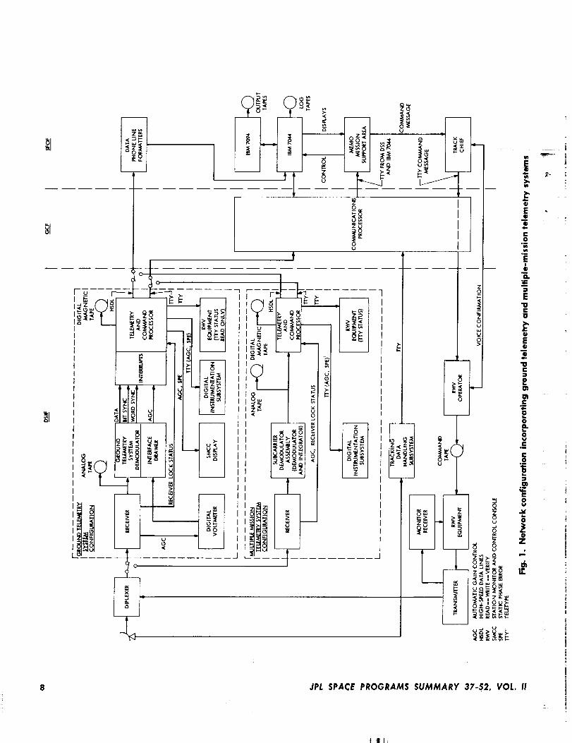
Figure 1 compares the configurations of the existing

ground telemetry system at the Mars DSS and the Robledo

DSS (the prime stations) and the newly developed

multiple-mission telemetry system at the DSSs committed

to the MEMO Proiect on a "best-effort" basis.

GCF support. The teletype data flow plan, preamble,

routing indicators, and channel assignments and the

circuit activation procedures for voice, high-speed data,

and teletype lines have been supplied to the DSSs. To

meet a Project request for real-time display of sciencedata at the Massachusetts Institute of Technology and

the Universities of Stanford, Iowa, and Colorado, tele-

type circuits with terminal machines are being provided.

SFOF support. The communications requirements for

the mission support area are defined and include a

requirement for a high-speed data switching interface to

some special mission-dependent equipment. The instal-

lation of equipment in the assigned mission support area

is essentially complete. The data processing system

input/output devices available to the MEMO Project

consist of two IBM 3070 printers, two 30 >( 80 plotters,

one input/output console, one card reader, and one

administrative printer.

The first of two software packages is the original

Mariner Venus 67 software, designated MOP. Only veri-

fication of its operational status is required. This software

package will be used at the DSSs equipped with the

Mariner Venus 67 ground telemetry system and in theSFOF.


I- <

( _i _ (_8_

.......... L

z

o

_m

0

v L

d0

_J

5_J

---I

b

r

1oE@

e.o

omIR

E

o.

E"ol=o

E@

"oi=

oO_

e,4,=

Eo

8.=.I=o

im4.

E=)

,m_4.

o_J

o

4)Z

iT.

|_

|

JPL SPACE PROGRAMS SUMMARY 37-$2, VOL. II

l|i

The second software package, designated MOPE, is

for use at the DSSs equipped with the multiple-mission

telemetry system. The operating features and output

formats of the existing MOP program are incorporated

in its design; thus, this program is entirely compatible

with the existing SFOF software. The functional relation-

ship of the existing MOP and new MOPE programs is

shown in Fig. 2.1

The hardware to be used in the monitoring area is

ready for operation. The following items are included:

two selective teletype machines, one IBM 3070 printer,

one addressable teletype machine, one Milgo Electronic

1The implementation plan and related details for the development

and testing of these programs was given in Oliver, E. F., Proiect

MEMO Software Compatibilities, April 23, 1968 (JPL internal

document).

Corp. printer and one input/output console. Residual

plot and print data will be available on a shared basis

with the Pioneer Project. Real-time monitoring opera-

tions will consist of telemetry and tracking data account-

ability and anomaly detection, telemetry data processing

update using reperforated tapes of tracking data, and

high-speed-data accountability and anomaly detection.Validation of tracking and telemetry data will be per-

formed as a non-real-time operation.

A new monitoring responsibility is the production of a

telemetry master data record (MDR), within 2 to 4 wk

of the corresponding station pass, meeting a defined setof criteria. All analog tapes, after return to the SFOF

with the corresponding digital telemetry-and-command-

processor data tapes, will be used to correct any defi-ciencies in the original data tapes. After being digitized,

the analog tapes will be validated together with the

TELEMETRY

STREAM

MULTIPLE

MISSION

TELEMETRY

MARINER 67

OPERATIONSPROGRAM

(MOP)

TELEMETRY

FRAME

SYNCSYSTEM

(MMTS)(TFS)

STATION

EQUIPMENTSTATUS

MMTS

MONITOR

OUTPUTS

(MMO)

I [ ITI

J'MOP (FROM MARl NER VENUS 67 SYSTEM)

IMMTS (FROM MARINER MARS 1969 SYSTEM)

MOPE = _MMO (FROM MARINER MARS 1969 SYSTEM

| PLUS ADDITIONAL INTERFACING)L.TFS (TO BE PROGRAMMED)

STATI O N

DISPLAYS

INPUT/OUTPUT

TYPEWRITER

IlI

II

I COMMUNICA-

I TIONS

I BUFFERIIII

I

()DIGITAL

MAGNETIC

TAPEi

AUTOMATICDATA

SWITCHING

SYSTEM

TELETYPE

LINE A

TO SFOF

TELETYPE

LINE B

HIGH-SPEED

DATA LINEt

Fig. 2. Functional relationship of MOP and MOPE programs


digital tapes, merged, reformatted (edited), and checked

prior to delivery of the master data record to the Project.

b. Validation/readiness testing and operations. Ground

telemetry system equipment integration tests and soft-

ware compatibility tests with MOP programs have been

performed at the Mars DSS and the Robledo DSS.In addition, DSIF configuration verification tests and

planetary ranging system tests were conducted at the

Mars DSS. It is expected that the ranging subsystem

will be operational when the spacecraft comes withinrange of the 210-ft antenna.

Remaining tests include MOPE software integration

tests and DSN readiness tests combined with operationalverification tests. Every effort was made to make the

design of the operations system as close to that of the

Mariner Mars I969 operations system as possible to pro-

vide some training for the subsequent Mariner Mars 1969

missions. Particular attention was devoted to the design

of the MEMO command system (Fig. 8).

Beginning in May, several attempts were made to

detect the Mariner V spacecraft signal using the 210-ft

antenna at the Mars DSS and special long-time integra-

tion techniques at the Venus DSS. Although these te_ch-

niques should have made possible the detection of signal

levels as low as -190 dBmW, the spacecraft signal wasnot detected as of June 18. It was concluded that un-

favorable polar diagrams due to the spacecraft's attitude

precluded the detection of a signal up to that time.

However, during the ensuing period, the spacecraft-earth

line would be moving rapidly around the spacecraft

antenna polar diagrams, and signal levels were expected

to increase rapidly. Efforts to detect the signal prior to

the scheduled operations on July 22 continued.

_r

VOIC

COMMAND MESSAGE

VOICE CONFIRMATION

TELETYPE

READ--WRITE--

VERIFY (RWV)EQUIPMENT

MONITORRECEIVER

TRANSMITTERRF SIGNAL

_I TRANSMITTER

Fig. 3. Command system configuration for MEMO Project


Itli

III. Advanced Engineering

A. Tracking and Navigational Accuracy Analysis:

DSN Inherent Accuracy Project

1. Introduction, r. w. Hamilton and D. W. Trask

The DSN Inherent Accuracy Project was formally

established by the DSN Executive Committee in July

1965. The objectives of the proiect are:

(1) Determination (and verification) of the inherent

accuracy of the DSN as a radio navigation instru-

ment for lunar and planetary missions.

(2) Formulation of designs and plans for refining this

accuracy to its practical limits.

Achievement of these goals is the joint responsibility of

the Telecommunications and Systems Divisions of JPL.

To this end, regular monthly meetings are held to coordi-nate and initiate relevant activities. The project leader

and his assistant (from the Systems and Telecommunica-

tions Divisions, respectively) report to the DSN Executive

Committee, and are authorized to task project members

to (1) conduct analyses of proposed experiments, (2) pre-

pare reports on current work, and (3) write descriptions

of proposed experiments. The project is further author-ized to deal directly with those flight projects using the

DSN regarding data-gathering procedures that bear on

inherent accuracy.

The various data types and tracking modes provided

by the DSIF in support of lunar and planetary missionsare discussed in SPS 37-39, Vol. III, pp. 6-8. Technical

work directly related to the Inherent Accuracy Project is

presented in SPS 37-38, Vol. III, and in subsequent Deep

Space Network SPS volumes, and is continued in the

following subsections of this volume.

Subsections 2, 3, and 4 discuss results obtained by

postflight analysis of tracking data from the Surveyor,Lunar Orbiter and Mariner V missions, respectively. Sub-

section 2 covers an intermediate stage of the post_flight

tracking data analysis for six of the seven Surveyor mis-sions. While the DSS locations obtained from the Surveyor

missions agree well with the combined Ranger solutions

(SPS 37-43, pp. 18-24), the Surveyor values are far more

consistent on a flight-to-flight basis than the Ranger

values were at a corresponding stage in the analysis. This

is probably due not only to the improvements made in

the DSIF tracking system between the Ranger and

Surveyor series of flights, but also to improvements in

both the lunar ephemeris and tropospheric refraction


model, as well as the fact that a heavy reliance was placed

on the values of GM_ and GM_ (the universal gravita-tional constants times the mass of the earth and the moon,

respectively) as determined from previous missions.

Subsection 3 discusses correlations between the major

visible lunar features and systematic variations in the

radio tracking data experienced with the Lunar Orbiter

missions. In SPS 37-51, pp. 28-37, it was demonstrated

that the variations in the doppler tracking data from theLunar Orbiter spacecraft are related to the sublunar track

of the spacecraft trajectory. This article discusses the cor-

relation of these residuals in a gross sense with major

visible features; namely, the maria and the highlands.

Data from spacecraft orbits with similar sublunar tracks

over the highland area show consistent variations with

relatively larger amplitudes than orbit tracks primarilyover maria.

An experiment designed to analyze error sources which

influence the doppler and ranging systems differently has

been previously discussed for the case of Lunar Orbiter

in SPS 37-44, pp. 28-33, SPS 37-46, pp. 23-38, and

SPS 37-48, pp. 4-7. It is envisioned that a calibration

technique can be devised to account for the effect of

charged particles in the ionosphere and space plasma,providing other error sources (such as the differential

variation in the electrical path length through the doppler

and ranging systems in the spacecraft transponder and

ground tracking station) can be independently removed

from the tracking data. However, to date this aspect of

the experiment has not been successful using either the

Lunar Orbiter data previously reported or data from

Mariner V, which is reported in Subsection 4. The

Mariner V data was obtained using the planetary ranging

system, which is an improvement over the ranging sys-tem used with Lunar Orbiter. At the same time, the

Mariner V spacecraft was in a far more stable environment

than the Lunar Orbiter, which at times passed through

the lunar shadow. However, differences between range

changes obtained by continuously counting the doppler

data and those obtained by differencing two range mea-

surements at the ends of this counting interval have been

observed which grow to 50 m over a 3-h interval. This

is far too large to be accounted for by charged particles

or any of the other effects investigated to date.

Subsections 5 and 6 are extensions of previously re-

ported work designed to gain insight into the ability to

navigate a distant spacecraft. The first of these continues

the analysis reported in SPS 37-51, pp. 37--41, which dis-

cusses the effect of target planet gravity on the estimate

of navigational accuracy for a deep space probe during

the planetary encounter phase. Approximate analytical

expressions are presented for the partial derivatives of

geocentric range rate of the spacecraft with respect to

the B-plane encounter parameters. The simplicity of

these expressions allows a quick insight into the geo-metrical properties of the spacecraft range rate prior to i

ithe planetary encounter and may be of considerable _: [value for rough calculations of navigational accuracy dur-

I

ing the planetary encounter phase. -t I|

The accuracy of the continuous minimum variance

estimate of the state of a distant space probe determined "

from a single pass of tracking data was discussed in

SPS 37-49, pp. 43--52. Subsection 6 extends this work for

several passes of data, and yields empirical formulas

which illustrate the geometrical influences on the accu-

racy of the estimates. The empirical formulas are accu-

rate for reasonable lateral velocities and are valid up to

about ten successive passes of data when the probe is

relatively free from planetary gravitational forces and

is at an appreciable distance from the sun.

The difllculty in accurately computing the long-termevolution of an orbit of an artificial satellite about a

central body and the importance of such calculations were

discussed in SPS 37-50, pp. 104-110, and an algorithm

for a numerical integration of orbital satellite "lifetime"

trajectories was reported. Subsection 7 describes a com-

puter program (IBM 7094 double-precision Fortran IV)

under development which implements this algorithm and

briefly discusses tile use and output of the program.

2. Deep Space Station Locations and Physical ConstantsSolutions of Surveyor Missions, s. K. Wong

a. Introduction. This article is concerned with an inter-

mediate stage of the post_flight analysis of the tracking

data from six of the seven Surveyor missions (Refs. 1, 2

and 3). The Surveyor II mission was omitted here because

of its incomplete flight to the moon. During the Surveyor

missions, primary tracking support was provided by the

Pioneer, Canberra, Johannesburg, and Madrid DSSs.

Some of the error sources which affect this analysis are:

(1) the limited numerical computational accuracy of the

single-precision orbit determination program (SPODP),

(2) discrepancies between the real universe and its model

in the SPODP (these include timing errors and polar mo-

tion effects; however, the polar changes for the translunar

trajectory are insignificant), (3) hardware errors, such as


I 111_

reference frequency instability and doppler counter error,

and (4) ephemeris error.

Timing errors between ephemeris time (ET, used to

locate the position of celestial bodies) and universal time

(UT.1, determined by the rotation of the earth and used

to fix the location of a DSS in space) may affect the orbit

determination process by misrepresenting the trajectory

of a probe _6th respect to the earth and other celestialbodies. Differences between UT.1 and Universal Time

Coordinated (UTC)/must also be reconciled in the orbit

determination processes, since the DSN synchronizes with

UTC and uses this time as a tag on the data received.

b. Discussion. The parameters estimated in the compu-

tations made to determine the best estimate of GM_,

GM¢ (the universal gravitational constant times the mass

of the earth and moon, respectively) arid station location

parameters for the Surveyor missions were: the spacecraft

position and velocity at an epoch; GM_; GM¢; the space-

craft accelerations [_, f._, and fa; the solar radiation con-

stant G; and two components (geocentric radius and

longitude) of station location for each tracking station.

The spacecraft nongravitational acceleration f_ is a con-

stant acceleration positive from sun to spacecraft; f: is a

constant acceleration positive in the direction normal to

the sun line with a component in the anti-Canopus direc-

tion; f_ is a constant acceleration in the direction required

to complete the right-handed orthogonal system. Only thetwo-way doppler data were used in the computations.

A priori 1-,r uncertainties of 100 m were used for station

location parameters, radius, and longitude. For GM, and

GM_, 1-_ uncertainties of 1.0 and 0.25 km'_/s 2, respec-

tively, were used. These values are approximately threetimes the 1-_r uncertainties associated with the combined

Ranger estimates.

In an effort to obtain the best estimate of the solved-for

parameters, the solution vector and its associated covari-

ance matrix, were used as a _riori information for the post-

midcourse maneuver data. The method of combining this

information is shown in Fig. 1.

q*_= q,, _ + q,, + aq.*, = best maneuver estimate

where

q,_ = nominal inflight maneuver estimate

q,,_ = U(q,)

'Broadcast by the National Bureau of Standards.

MIDCOURSEMANEUVER

BL_ 2ql ql,2 IMPACT

INJECTIO_

Fig. 1. Method of combining premidcourse and

postmldcourse phase

q2 = solution vector of estimated parameters from

block 2 (from midcourse maneuver to impact)

data only

aq_ = (A_Wa: + a-' _ ,[a_ w (o, - c_)1,21

+ a;_,=(q,,= - q_)]

and

observable in block 2

Aa = a estimated parameter

O_- Ca = residuals (i.e., observed data minus calcu-

lated data; block 2)

q_ = solution vector of estimated parameters

from block 1 (from injection to midcourse

maneuver) data only

U = matrix which maps q, to postmidcourse

epoch

W = diagonal weighting matrix on observables

A1,2 = UA1U v + A_

A,_ = covariance on maneuver (diagonal pur-

posely set to a very pessimisti c value of

100 m/s)

a, = (a,_wa, + 7,-9-'= covariance on estimated parameters from

block i data only

"A= a priori eovarianee matrix

Spacecraft orbital elements and physical constants esti-

mated from range rate (doppler) data are influenced by

tropospheric refraction. The SPODP includes an equationto correct the data for this effect, as follows:

_b = 3_ sin F + B) TM (sin C + B) _'i

JPL SPACE PROGRAMS SUMMARY 37-$2, VOL. II 13

Table 1. Station locations and parameters (referenced to 1903.0 pole)

Data source r,, km

Mariner II

Mariner IV, cruise

Mariner IV, post-encounter

Pioneer VI, Dec. 1965-June 1966

Goddard ]and survey, Aug. 1966

Surveyor I, post-tauchdown

Surveyor Ill, in flight

Surveyor IV, in flighl

Surveyor V, in flight

Surveyor VI, in flight

Surveyor Vii, in flighl

Mariner IV, cruise



Gaddard land survey, Aug. 1966

Surveyor 1, post-touchdown

5206.3357

r, 1--_ standard

deviation, m

_, 1-o" standard Geocentric

_,, deg deviation, m radius, deg

8.8 6372.0044

Surveyor 111, in flight

Surveyor IV, in flight


Surveyor VII, in flight

.3404

.3378

.3359

.3718

.3276

.3408

.3326

.3256"

3.9

Pioneer DSS

243.15058

Geocentric

latitude,

deg

.3337

.3359

10.0

37.0

9.6

29.0

2.9

29.7

41 .I

47.0

067

072

092

094

085

100

097

092

20.0

40.0

10.3

35.0

23.8

49.0

49.0

39.0

.0188

.0161

.0286

.0640

.6446

--.0230

.0129

.0043

35.208035

08144

08151

08030

08230

16317

08192

08192i

! 08192

Combined Rangers, LE 3 b

Ranger VI, LE 3

Ranger Vfl, LE 3

Ranger VIII, LE 3

Ranger IX, LE 3

Mariner IV, cruise



Goddard land survey, Aug. 1966

Surveyor I, in flight

Surveyor III, in flight

Surveyor IV, in flight

Surveyor V, in flight



_r

30.3

26.1

091

086"

43.0

-- 36.0

.0141

.0164

5205.3478

.3480

.3384

.2740

.3474

.3522

.3487

.3501

10.0

t

Tidbinbilla DSS

20.0

,qp

6371.6882148.98136

qf .3445

28.0

5.0

52.0

3.5

26,5

34.8

24.6

134

151

000

130

146 °

161

153

29.0

8.1

61.0

22.1

45.0

49.0

45.0

.6824

.6932

.7030

.6651

.6905

.6861

.6879

08182

qr 08184

--35.219410

19333

19620

20750

19123

19372

19372

19372

Lunar Orbiter II, doppler

5742.9315

.9203

.9211

.9372

.9626

.9363

.9365

.9332

.9706

.9380

.9312

.9337

.9355

.9413

Ir .9309

¶_ 1936827.1 _ r 156 35.0 _ .6807

Johannesburg DSS

6375.5072 --25.739169

40.0

11.6

39.0

38.3

35.0

39.3

44.1

25.6

32.5

3.5 27.68572

19.7 : 572

25.5 583

22.3 548

56.6 580

10.0 540

557

569

586

578

574

575

574

57O

_11' 573

Robleda DSS

22.2

69.3

61.3

85.0

49.5

20.0

38.0

12.0

43.0

41.0

46.2

46.8

31.5

43.0

36.7 I,

Lunar Orbiter II, doppler and

ranging



Surveyor Ill, in flight


4862.6067

.6118

.6063

.6059

.6054

r .6O62

9.6

3.4

14.0

8.8

24.5

27.3

355.75115

138

099

103

126

Ir 129

.4972

.4950

.5130

.5322

.5120

.5143

.5094

.5410 i

.5144 !i

.5069 ii

.5096 iI

.5116

.5180

.5062 _r

aThls number is questionable because af passible error in the station data.

bjp/ lunar ephemeris 3 (DE 15); all Surveyor in-flight solutions used JPL lunar ephemeris 4 (DE 19).

J 9215

9157i! 9159ii 8993

i 9148ii 9198

! 9176

8990

9169

9169

9169

9169

9169

9165

40.238566

38566

44.4 6369.9932

4.0 69.9999

24.0 70.0009

10.4 70.0060

47.0 70.0046

39.0 I f 70.0050

38655

38715

38701

_f 38701

, !k-


Iil

where

A -- 0.0018958

B = 0.06483

F = _ + (r/2)

G = 7 -- (r/2) -/

N_ = index of refraction of station i

-/-- elevation angle, deg

r -- doppler averaging time, s

The SPODP "canned" value of N_ is 340 for all stations.

However, improved values have been provided (A. S. Liu,

SPS 37-50, Vol. II, pp. 93-97) and used for this study.

They are:

DSS N_

Pioneer

Tidbinbilla

JohannesburgRobledo

240

310

240

300

The ephemeris used for this study was JPL develop-

ment ephemeris 19 (DE 19), which has incorporated the

updated mass ratios and Eckert's corrections (Ref. 4).

c. Results of station location solutions. The results of

these computations are presented in Table 12 in an un-

natural station coordinate system (geocentric radius, lati-

tude, and longitude) and in a natural coordinate system

(r,,),, Z), where r_ is the distance off the earth spin axisin the station meridian, )_ is the geocentric longitude, and

Z is distance along the earth spin axis. Figures 2-9:' show

the station locations obtained for Surveyor missions as

compared to other various missions. Likewise, Figs. 10-12indicate results for the relative locations. The first set of

figures show that the range of values of the station loca-

tion parameters obtained from Surveyor missions is asshown in Table 2.

If three estimates were omitted from the list (Table 1)

the range of station location parameters would be asshown in Table 3.

:Values for missions other than Surveyor were obtained from Ref. 1.

'Terms used in Figs. 2-12: REF. --- referenced; DOP. --- doppler;

CR. = cruise; COMB. = combined; PE = post-encounter; PT =

post-touchdown; LE - hmar ephemeris; LO -- Lunar Orbiter.

S-

Table 2. Range of values of station location

parameters

DS5

Pioneer

Tidbinbilla

Johannesburg

Robledo

Range of values, m

Ar, Ah

15 14

7 15

10 8

0 3

Table 3. Range of values of station location

parameters omitting three estimates

DS5

Pioneer

Tidblnbilla

Range of values, m

Ar, AX

8 9

7 8

5206.38

5206.36

5206.34

5206.32

5206.30

5206.28

m

m

I

B -

_i

U tJ t.) L) U

- _ = > > > _,

(5

d_

Ou_u

Fig. 2. Distance off spin axis (earth-fixed

system, 1903.0 pole, Pioneer DSS)


"13

uS

2(3Z

16

243.1514

243.1512

243.1510

243.1508

243.1506

243.1504

I I

_ U U U U U

- _- _ >- =

>

o_.u

Fig. 3. Geocentric longitude (earth-fixed system,

1903.0 pole, Pioneer DSS)

Fig. 5. Geocentric longitude (earth-fixed system,

1903.0 pole, Tidbinbilla DSS)

E

S-

u;cJ

(3Z

2

5205.38

5205.36

5205.34

5205.32

-B -

> _ u u u u

_ 0 > >z__

> >- >- >- >.

Fig. 4. Distance off spin axis (earth-fixed system,

1903.0 pole, Tidbinbilla DSS)

148.9820

148.9818

148.9816

148.9814

148.9812

148.9810

i

J

-Ii --

J

U U U U

o_> _ = > > >--


q

ii

5742.98

5742.96

5742.94

5742.92

5742.90

I-"I

I--

ii

Fig. 6. Distance off spin axis (earth-fixed system,1903.O pole, Johannesburg DSS)

27.6862

27.6860

-_ 27.6858

u2D

0Z

_ 27.6856

27.6854

i

i

-0 27.685 ......._ _> => => => >_ _ > =- = > > -=_ _ > >

0 _ _ _a a a a a a _z_ z _ o o._ o 8U0 _ Z _ _ >- >- ,_, >_ ,_.

D D D

0U

Fig. 7. Geocentric longitude learth-fixed system,

0903.0 pole, Johannesburg DSS)

Fig. 8. Distance off spin axis (earth-fixed system,1903.0 pole, Robledo DSS)

4862.64

4862.62

4862.60

4862.58

t-..

I I

>_

z um

_q

i

i

_J

_=_

G _

o

JPL SPACE PROGRAMS SUMMARY 37-52, VOL. Ii17

,2

D

Z

2

355. 7518

355.7516 r355. 7514 J J

355.7512

355. 7510

355. 7508

a2Z u

[]

• °

Z

_ _ >

> >"a au

_qo

Fig. 9. Geocentric longitude (earth-fixed system,1903.0 pole, Robledo DSS)

These three estimates are:

(1) r8 for Pioneer DSS; Surveyor V.

(2) X for Pioneer DSS; Surveyor VII.

(3) X for Tidbinbilla DSS; Surveyor IH.

For this study the obvious biased data or erroneous datahad been removed. The observed minus computed re-

siduals indicate possible errors in the Pioneer DSS datafor Surveyor V and VII missions. A more detailed analysisof Pioneer DSS data is required to determine this error.The estimated value of Tidbinbiiia DSS geocentric longi-tude for Surveyor III appears to be slightly low when

compared to the other Surveyor missions. This is probablydue to the removal of 7 h of Robledo DSS biased near-moon data between Tidbinbilla and Pioneer DSSs.

The range of values indicates that consistent stationlocations were obtained from the Surveyor missions. The

uZ

Ud

6

.d

94.1698

94.1696

94.1694

94.1692

94.1690

-!

m

m

_. _ d d d d> _ u t,J u u

- _ -__ >_

Z_, > >- >- >.

Fig. 10. Geocentric longitude differences (earth-

fixed system, 1903.0 pole, Pioneer DSS values

minus Tidblnbilla DSS values)

weighted mean of r, and A for Pioneer DSS differs only

by 4.8 and 4.3 m, respectively, from the combined Rangerestimates _ referenced from Echo DSS. The weighted meanof r, and X for Johannesburg DSS also differs by only 4.3and 2.4 m, respectively, from combined Ranger estimates.

d. Results of physical constant solutions. The estimates

of GMe and GM_ for the Surveyor missions are presentedin Table 4. Figures 13 and 14 show how well the GMe

and GM_ estimates obtained from the Surveyor missionscompare to the estimates obtained from other missions.The results indicate that the Surveyor missions contributelittle information to the GM_ estimate, since the 1-e uncer-tainty associated with the Surveyor GM_ estimate de-

creased from the input a priori by only a very smallamount. The values obtained for GMe range from39860i.10 to 398601.27 km3/s 2. The average GMe value(39860L16 km_/s 2) for the Surveyor missions is only0.06 km3/s 2 from the combined Rangers estimate.

_Obtained using JPL lunar ephemeris 3.

1-


II11¸

g,"o

uz

t_

0z

q

215.4656

215.4654

215.4652

215.¢650

215.4648

215.4646

7I

Nm

m

> u u u u u- _ > -_ >

°zz_S_ _

0u

Fig. 11. Geocentric longitude differences (earth-fixed

system, 1903.0 pole, Pioneer DSS values

minus Johannesburg DSS values)

e. Conclusion. The station locations and physical con-

stants obtained are consistent between Surveyor missions

and are in agreement with the estimates of other missions.However, some differences are expected between the

Surveyor estimates and estimates of other missions for

the following reasons:

(1) Surveyor used an S-band tracking system, whereas

missions such as the Rangers used an L-band track-

ing system.

(2) Surveyor estimates were computed with a new setof indices of refraction.

(3) Differences in the physical constants used in the

trajectory (SPACE) program.

(4) An improved version of the ephemeris was used in

Surveyor orbit computations.

There are no physical phenomena that justify estimat-

ing the spacecraft nongravitational accelerations [_, ]c, f_.

-10

t.)Z

m

25Z0..J

121.2962

121.2960

121.2958

121.2956

121.2954

_ddddu u u u

>--=>>N

Fig. 12. Geocentric longitude differences (earth-fixedsystem, 1903.0 pole, Tidbinbilla DSS values

minus Johannesburg DSS values)

Table 4. Physical constants and statistics

Data source

Lunar Orbiter I1"

{doppler)

Lunar Orbiter III

{doppler and

ranging)

Combined

Rangers b

Ranger VI

Ranger VII

Ranger VIII

Ranger IX

Surveyor I

Surveyor Ill

Surveyor IV

Surveyor V

Surveyor VI

Surveyor VII

GM e,kmS/s =

398600.88

398600.37

398601.22

398600.69

398601.34

398601.14

398601.42

398601.27

398601.1 I

398601.19

398601.10

398601 .! 1

398601 .I 1

GM e 1-_,Standard

deviation,

km_fs =

2.14

0.68

0.37

1.13

1.55

0.72

0.60

0.78

0.84

0.99

0.60

0.54

0.80

GM(,km_/s _

4902.6605

4902.7562

4902.6309

4902.6576

4902.5371

4902.6304

4902.7073

4902.6492

4902.6420

4902.6297

4902.6298

4902.6425

4902.6429

GM( 1-eStandard

deviation,km_/s _

0.29

0.13

0.074

0.185

0.167

0.119

0.299

0.237

0.246

O.247

0.236

0.235

0.235

• Lunar Orbiter values were obtained from SPS 37-48, Vol. II, pp. 12-22.

_'Ranger valuel were obtained from SP5 37-44, Vol. III, pp. 11-28.


eq

o

398603

398602

398601

3986OO

398599

I-1!!-

/

-I!

mm

i

J

-i

m

m

tm

m

z _@z _ _ _ _

oU

..,I .-J

Fig. 13. Comparison of GMe estimates

However, when these accelerations are estimated, the fit

on the near-moon data is significantly improved. This

seems to indicate that solving for spacecraft acceleration

compensates for the near-moon orbit-determination-

program model inadequacies. Efforts are being continued

to improve this set of estimates and publish a set of com-

bined Surveyor station locations and physical constants.

References

1. Thornton, T. H., Jr., et al., The Surveyor I and Surveyor 1I

Flight Paths and Their Determination From Tracking Data,

TR 32-1285, Jet Propulsion Laboratory, Pasadena, California

(in process).

2. O'Neil, W. J., et al., The Surveyor III and Surveyor 1V Flight

Paths and Their Determination From Tracking Data, TR 32-

1292, Jet Propulsion Laboratory, Pasadena, California (in

process).

3. Labrum, R. G., eta]., The Surveyor V, Surveyor VI, and

Surveyor VH Flight Paths and Their Determination From

Tracking Data, TR 32-1302, Jet Propulsion Laboratory, Pasa-

dena, California (in process ).

4. Eckert, W. ]., and Smith, H. F., Jr., Astronomical Papers of the

American Ephemeris, Vol. 19, Pt. II. Nautical Almanac Office,

U. S. Naval Observatory, U. S. Government Printing Office,

Washington, D. C.

(.9

4903.0

4902.9

4902.8

4902.7

4902.6

4902.5

4902.4

FI

i -

/1

_ °z _ _ z =z _ ==

0U

Fig. 14. Comparison of GM_ estimates

3. Correlations Between Major Visible Lunar Features

and Systematic Variations in Radio-Tracking Data

Obtained From Lunar Orbiter III,

W. L Sjogren and P. M. Muller

In SPS 37-51, Vol II, pp. 28-37, it was demonstrated

that the variations in the doppler tracking data from the

Lunar Orbiter HI spacecraft are indeed related to the

sublunar track of the spacecraft trajectory, and mention

was made that there was some correlation between the

tracking data and major visible lunar features. These

visible features are essentially two gross areas, namely,

the maria and the highlands; the maria being Mare

Nubium and its adjacent maria and the highlands being

the area between zero and 30 deg east longitude and

zero and 30 deg south latitude. Data from spacecraft

orbits with sublunar tracks over these areas show con-

sistent variations with relatively larger amplitudes than

i1

i


those of other orbit tracks, primarily those over certain

maria.

Such tracks are displayed in Fig. 15 where tracks a

and b are over maria and highland, and track c is pri-

marily over maria. The variations in the doppler data for

the three different tracks, after differencing with a fit to

a theoretical universe model having a triaxial moon, are

shown in Fig. 16 (i.e., residual plots). Of course, the

amplitude of the residuals is dependent on the altitude h

of the spacecraft over the features (proportional to l/h=),

but the primary correlation to note is the slope of theresidual, for it is the direct measure of the acceleration

produced by some mass distribution. A positive slope on

N80° 80°

7 " - - 70°

-70* "_-_-_--_-=_-' _ -_ %-_-'-r+_ _--0.__-70o

_80 ° ..... --__ _80 °S

Fig. 15. Lunar map showing Lunar Orbiter III orbit tracks


.J<

C)m

0c_

2.0 --

1.5

1.0

0.5 --

-0.5

-I.0

-I .5

-2.0

0

I ITRACK a

EPOCH: 8/30/67, 20: 56:32 GMT

223

-30

ALTITUDE = 153 km

LONGITUDE = 33 deg

LATITUDE = -I I degi

_r

304

-95

-8

284-75-14

-21 ......

ek

_.K.K.t(..Ik243

-44

-20

_r

t(- 1_

180

3

"18

MARE |

iF NUBIUM-_

HIGHLANDS -i

i ISEMIMAJOR AXIS = 1968 km

ECCENTRICITY= 0.06

! Hz = 65 mm/$

14647

tk

148

75

4

145

64

0

.w

.)e

L.le 'N"

10 20 30 40 50 60 70 80

TIME FROM EPOCH, rain

Fig. 16. Lunar Orbiter I1| doppler residuals


It!!

f

1.5

1.0

0.5

-0.5

-! .0

-I .5

1 ITRACK b

EPOCH: 9/18/67, 14: 36:32 GMT

240

-70

16

tl. '11"t_"Ntl"

314 --

-17

-2

N"_. "_tl6tt"

267 294 _e

ALTITUDE = 304 km

LONGITUDE = 39 deg

LATITUDE = -19 deg __

tq. II" I't_

ti-

-51 -36

10 5

-_ HIGHLANDS-_

213

101

-18

tl-

t(- tl-

269

67

,91

0 10 20 30 40 50 60 70 80

TIME FROM EPOCH, min

Fig. 16 (contd)

the residuals indicates a positive acceleration. In both

Figs. 15 and 16, particularly in the longitudes of the

tracks a and b, a definite correlation is apparent between

the slopes of the residuals when the spacecraft is passing

over a mare (negative) and when it is passing over a

highland (positive)-the highlands produce an increase

in velocity. These two tracks are representative of many

orbits over these areas; all of which display these samecharacteristics.

If the assumption is made that the disturbing mass

causing the positive acceleration in the highland area for

tracks a and b (both tracks are rather close in this area)

is the same, then an approximation to an effective mass

depth can be calculated by the relationship that the

acceleration is proportional to 1/h z, where h is the alti-

tude of the spacecraft above the mass center. The result-

ing depth is some 30 km below the mean radius of 1738,

and the corresponding mass is approximately 0.5 >( 10 6that of the entire moon.

These are gross features, since even craters like

Copernicus are averaged out in each data sample. The

data are averaged over 1 min, and in that time the space-

craft has traveled 100--120 km, the entire spread of

Copernicus. The features mentioned here cover 600-

1000 km. However, in analyzing higher sample rate data

(1/10 s), no systematic effects were seen within the noiselevel of 0.5 mm/s.

Presently data reduction is proceeding on some polarorbits. The initial review of the results shows good cor-relation between the residuals and the sublunar track.

The regions of Mare Imbrium and Mare Serenitatis dis-

play high amplitude accelerations, presumably caused by

submerged mass distributions. Analysis of the data should

give an estimate of this distribution.

JPL SPACE PROGRAMS SUMMARY 37-52, VOL. I! 23

,,=.

2.0

1.5

1.0

0.5

0

-0.5

-1.0

-I.5

0

I 1TRACK c

EPOCH: 9/5/67, 16: 40:00 GMT

137 133

-46 -23

-10 -2

tttt _ _t

t

tt

..N..,_._"!160

-72

-18

ti.

t

----- 155

11

10

tt.K-

,N-

.t

t&t

t .N.

I*t137

-11 --

2

ALTITUDE = 235 km

LONGITUDE = 67degLATITUDE

177'

29

16

t(- 1_t

tl-

2O3

19

= 21dee

-IN te

•_ .t tel.

t

t.t

tIPtt_

28_

98

19

_tl .tt

tl.

10 2O 30 40

TIME FROM EPOCH, rain

Fig. 16 (contd)

50 60 70 80

24 JPL SPACE PROGRAMS SUMMARY 37-52, VOL. I!

I]11

4. Mariner V Differenced Range-Integrated Range

Rate Experiment, F.s. Winn

a. Introduction. The doppler-ranging calibration ex-

periment was designed to analyze error signatures which

influence doppler and ranging systems differently. Under

the assumption that the ionospheric charged particle

effects constituted the preponderance of error signature,

the experiment was to provide the means to measure

charged particle effects on the data. Liu (SPS 37-48,

Vol. II, pp. 30-37) was the first to attempt to solve this

problem, utilizing Lunar Orbiters II and IV ranging and

doppler data sets. The results of that effort are similar tothe conclusions of this article. To date, the self-contained

calibration inherent to the data pair, ranging and doppler,

has been unusable, in that other unknown larger error

signatures have contaminated the data samples.

b. Analysis. Mars DSS received tracking data from the

Mariner V probe at one voltage-controlled oscillator

(VCO) setting during each of the following time periods:

GMT 1967

Pass From To

day:h:min day:h:min

27 191 :19:32 191:21:51

39 203: 21:02 203: 22:54

40 204:19:42 205:01:53

The tracking data types acquired were by research and

development planetary ranging units (PRU) (SPS 37-42,

Vol. III, pp. 52-56) and coherent two-way doppler (CC3)

(Ref. 1).

The net mean difference between PRU and CC3 for

consecutive minute intervals throughout the durations

of the three passes was computed (SPS 37-44, Vol. III,

pp. 28-33) from the following expression

5 = {R, -- R,- (K/fq) [(CC3t - CC3,) - 106 (Tt- T,,)] } C

CC3t

where

/l_ = octal range converted to decimal at initial

time (round-trip range, s)

Rt : octal range converted to decimal at time t

(round-trip range, s)

CC3_ = cumulative doppler count at initial time,

cycles

= cumulative doppler count at time t, cycles

Tt -- T_ = time interval of time t minus initial time, s

K = (240/221)

f_ = VCO frequency

C -- velocity of light, m/s

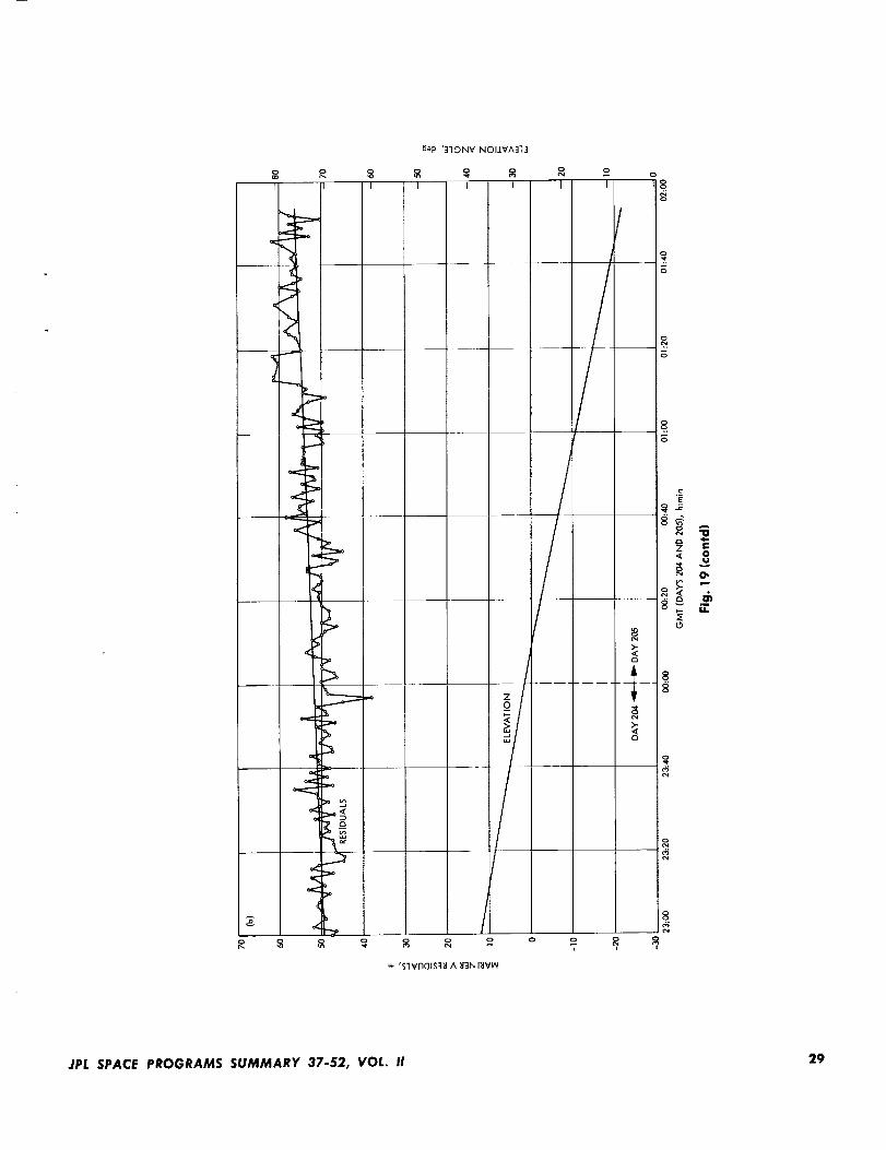
The irregular A function profiles are depicted in

Figs. 17, 18, and 192 The profiles represent the disagree-

ment in range change between the PRU and integrated

CC3 data types. The smooth curve is the probe's eleva-tion relative to the Mars DSS astronomical horizon.

c. Charged particle effects. Both data types, PRU and

CC3, are affected by the charged particle concentrations

characteristic to the space plasma and ionosphere medi-ums. Electron mediums retard the ranging signal (group

velocity) and advance the doppler signal (phase velocity)

(Ref. 2). The magnitudes of these influences on the two

data types are equal and opposite. The magnitudes of

the effects are directly dependent upon the effective num-

ber of electrons along the ray path. It was the primary

purpose of this experiment to evaluate the charged par-

ticle influences, but, as will be shown, other systematic

error sources are masking over the sought-after signature.

d. Space plasma. The total electron count to which the

data types were subjected can be ascertained. Mean inter-

planetary medium plasma electron densities at a helio-centric distance of 1 AU were found to be between 5 and

10 electrons/cm '_by plasma detectors aboard Pioneers VI

and VII (Ref. 3). If 8 electrons/cm _ is adopted as a mean

electron density, 6 the 107-km earth-probe distance for

pass 40 would produce only a 1.6-m difference betweenthe PRU and CC3 data types.

e. Ionosphere. Ionospheric electron content historiesare derived from the Stanford Radio Science Laboratory

Applied Technology Satellite Faraday rotation measure-

ments. Figs. 20 and 21 show the ionospheric electroneffective total counts for the Mars DSS Mariner V sub-

ionospheric points.

(_) Zenith slant range total electron count history.

(_) Slant range total electron count history for

Mariner V meridian passage subionospheric point.

BProgramming by R. N. Wimberly.

_Pioneer VI plasma detectors measured a mean electron density ofless than 10 electrons/cm a on Day 204 (private communicationfrom Taylor Howard, Stanford Radioscience Laboratory).


-- o__... °

cd7

cC

E

fl

v-_ u

.2

C

.E 14.

0 _0

a.

i


I|1

5O

E3O

MARS DSS

15 cycles _ 1 m

2O

>

Z

io

0

ELEVATION

-1021:00 21:20 21:40 22:2022:00

GMT (DAY 203), h: mln

22:40

70

Fig. 18. Pass 39, Day 203, 1967 A function profile

6O

20

23:00

50

40

30

(_) Slant range total electron count history for the

Mariner V acquisition subionospheric point.

(_) Slant range total electron count history for the

Mariner V termination subionospherie point.

The broken profile is the ionospheric charged particle

influence on the a function (10 _7electron = 1 m). Fig. 21

shows that a 7-m retardation of the ranging code coupled

with a 7-m advance of the doppler signal will provide a

14-m maximum magnitude for the pass 40 _ function. Not

only does the maximum magnitude as indicated by the

ionospheric study fall far short of the computed differ-

ences of the observables, but the ionospheric signature

does not resemble the a function profile. Similarly, the

pass 27 _x function does not correlate with the ionospheric

density profile. Although the ionosphere is known to be

a significant influence on the _x function, it is not the

primary influence to which the available data samples

were subjected.

f. Mariner V ranging transponder delay. Ranging tran-

sponder delay characteristics as functions of temperature,

signal-to-noise ratio, and transponder frequency offset

have been investigated. The Mariner V calibration in

conjunction with the known temporal environmental and

operational influences on the probe indicates that the

spacecraft's hardware did not induce any significant

retardation to the ranging code.

g. Temperature-dependent ranging delay. The calibra-

tion of temperature influence on the ranging transponder

shows a constant 900-ns ranging code delay through the

radio subsystem in the temperature range of 50 to 100°F.

Figure 22 shows the temperature history of the probe with

the near-constant temperatures of passes 27, 39 and 40

indicated. (These temperatures are regarded as fixed for

any of the pass intervals.) On the basis of this evidence,

transponder temperature variation is excluded as a pos-

sible cause of the differenced range-integrated range rateresiduals.

h. Ranging transponder delay-frequency-offset-

dependent. The Mars DSS has a ,spin axis distance of

5204 km, and thus the station has a 400-m/s rotation

velocity. At S-band frequencies this diurnal rotation ve-

locity amounts to a 7.4-kHz doppler shift for the pass 40

tracking period. The frequency offset-ranging tran-

sponder delay calibration (Fig. 23) indicates that the

induced transponder delay which corresponds to a fre-

quency offset is only 4.2 >( 10 -5 m/Hz.. Thus, a 7.4-kHz

offset will result in a ranging transponder delay of only0.3 m.


6_p ']IONV NOI/VA:I]:I

t

i >

7>a

xx_

1

i

IIi

7Ii

o

c

ZC

,<>

/

ac.;_ !

%:o o9_ o

_E

e_

C

0

C

O,

0

4o

>..0

0

0

_L


l|i

.o

7q

m

6ap ']IDNV NOIIVA]I]

I I I I I I

_L

/

Z

o

iw 'slvnals]_ ^ _]NI_VW

o

o

>.<r_

>.

E

0


r%

o

x

o

w¢D

UZ

3

u_

12

\

0 4 8 16 20

PST (JULY 11, 1967), h

24

Fig. 20. Ionosphere electron concentration for Mars DSSMariner V subionosphere point (Pass27, Day 191, 1967)


III

2O

ox

u3 12/z i

/

__ /

9 8 //

U

4

" PASS40 =

00 4 8 12 16 20 24

PST(JULY 24, 1967), h

Fig. 21. Ionosphere electron concentration for Mars DSS Mariner V subionosphere point (Pass 40, Day 204-205, 19671


o"

65

75

70 ........

UL

6O0 20

I

JULY 1, 1967

/_p PASS 39

ASS 40

40

tAUG 1

f

j 68

60 80

ISEPT 1

TIME FROM LAUNCH, days

100

IOCT 1

120

Fig. 22. Mariner V temperatures

140

iI

tI

t


1|1

2.0

1.5

1.0

0.5

E

0r_7

£

-0.5

-1.0

-1.5

-2.0

0

1-Hz OFFSET = 4.2 x 10-5 rn

o//

TRANSMITTED FREQUENCY V T =Vvc O x 96

100 200 300 400 500 6OO 700

VCO FREQUENCY Vvc O , Hz ABOVE 22,030,800 Hz

8OO 9OO

Fig. 23. Mariner V ranging transponder delay versus transponder frequency offset (static phase error)


i. Ranging transponder delay- signal-to-noise.

dependent. The signal to noise (S/N) level ranging-

transponder delay calibration shows an 8.4-ns delay change

in the ranging transponder circuit travel time/dBm unit

change in the S/N. This linear relationship could pro-duce the A function's 48-m bias between the PRU and

CC3 data types associated with pass 40 if the S/N varied

by 19 dBm; however, telemetry channel data shows the

S/N to vary only 0.7 dB between -118.9 and -119.6dBm. This small variation results from the attitude-control

system limit cycle, and can be viewed in Figs. 17, 18,

and 19 as small periodic excursions of the /x function

(_2-m amplitude).

i. Conclusion. All efforts to correlate the differenced

range-integrated range rate differences with the physical

phenomena investigated have failed. The difference func-

tion (a) profile and magnitude do not correlate with

ionospheric charged particle effects, transponder tem-

perature changes, signal-to-noise variation or transponder

frequency offset (static phase error). If the medium and

transponder are excluded as the primary error signature

contributors, then by exclusion the terrestrial hardware

system is the indicated source.

An investigation of the research and development

planetary ranging system hardware has revealed that

some of the system's modules are subject to phase drift, rPRU and CC3 data will be collected when Mariner V is

again within range this fall. Efforts will be made to moni-

tor the phase drift between the research and development

planetary ranging system's transmitted and received fre-

quencies; thus it should be possible to calibrate out of the

data any system-induced phase drift.

References

1. Lorell, J., Andcrson, J. D., Sjogrcn, W. L., Characteristics andFormat of the Tracking Data to Be Obtained by the NASA DeepSpace Instrumentation Facility for Lunar Orbiter, TechnicalMemorandum 33-230, Jet Propulsion Laboratory, Pasadena,Calif., June 15, 1965.

2. Stratton, J. A., Electromagnetic Theory, McGraw-Hill Book Co.,New York, 1941.

3. Koehler, R. L., Interplanetary Electron Content Measured Be-tween Earth and the Pioneer VI and VII Spacecraft Using RadioPropagation Effects, Scientific Report 1_Stanford Radio ScienceLaboratory, Stanford, Calif., May 1967.

_Private conversations with R. C. Tausworthe and R. Tappen.

34

5. An Approximate Solution to the Analytical Partials

of the Spacecraft's Geocentric Range Rate During

the Pre-encounter Phase of a Planetary Mission,W. E. Bollman

a. Introduction. The simple analytical expressions for

the planet-centered position and velocity vectors of the

spacecraft while in the vicinity of the target planet were

introduced in SPS 37-51, Vol. II, pp. 37-41. This article

will continue the analysis to show approximate analytical

expressions for the partial derivatives of geocentric range

rate of the spacecraft with respect to the encounterA Cx

parameters b- T, b" R, Te, C3, S" T, and S" t_.

b. Background. The previously mentioned SPS article

presented the target-planet-centered position and velocity

of the spacecraft to be

/', _'N A

R_/p ----R_/p [cos a S + sin _ cos 0 T + sin a sin 0 R]

(1)

t[£ A

where

/z A

+ _ (cos a -- 1) cos 0 T

(9)

/_ (cos,-- i) sin0+

b z

Voo =

0=

b _V_R_/_- (3)

_,(i +bv:_ sin.-cos.)

A

S = unit vector along the approach asymptote¢N

T = unit vector perpendicular to S and parallel to a

given reference plane (such as ecliptic) and given

byA A

^ SXP

IA

where P is along north pole of reference plane

= planet-centered angle from -S to R,/p

the miss parameter

the hyperbolic excess speed

the gravitational constant of the planet

the orientation of the trajec_ry aiming point, mea-sured clockwise from the T axis to the miss pa-rameter b.


I|i

A

S

/

LANE

A

T

Fig. 24. Hyperbolic encounter parameters

Figure 24 shows a diagram of some of the above pa-rameters.

The angle a, presented in Eqs. (1), (2), and (3) and in

Fig. 24, remains a very small angle prior to planet en-counter until the spacecraft is within an hour or so of

closest approach. This characteristic enables approximate

expressions to be easily derived for the partial derivatives

of geocentric range rate with respect to the encounter

parameters that are accurate during the pre-encounter

phase of the mission.

c. Geocentric range rate. The geocentric range rate of

the spacecraft during the planetary phase of the mission

can be expressed as

_--(Rp + R vp)"_ (4)

where

R_ _- the position vector from the center of the earth

to the planet

Rs/p = the position vector from the planet to the space-craft

Ar --- the unit vector from the center of the earth to

the spacecraftA

r = r r = (R_ + Rs/p)

Figure 25 shows a graphical explanation of some of the

above parameters.

d. Encounter parameters. The encounter parameters to

be used in this analysis are as follows:A

b.T--bcos0A

b" R -- b sin 0

Te = time of closest approach

C_ = V_A

S" T = dot product of new perturbed S vector with oldnominal T vector

A ]x /N

S • R : dot product of new perturbed S vector with oldnominal R vector


EARTH

Fig. 25. Geocentric range-rate vectors

e. Partial derivatives. Taking the partial derivative of

Eq. (4) with respect to the encounter parameter, e.g., q,yields

_q: _ + _ _ (5)

where

A A.

q = b'T,b'R, C3, etc.

The total partial deriva_ve is thus the sum of twoexpressions. When q- b" T and b" R, it is found that

the first expression of Eq. (5) is nearly a constant during

the pre-encounter phase and usually dominates the sec-

ond expression until a few hours or a few days before

closest approach, depending on the target planet and the

approach trajectory, at which time changes of the space-

craft's velocity then become more noticeable from per-

turbations of the encounter parameters. The velocity ofthe planet with respect to the earth, Rp, does not depend

on the encounter parameters and is almost constant dur-

ing the few-day period when the spacecraft approaches

the planet.

The approximate partial derivatives which are valid

when the angle a is small are

1+ v=)(_, s) (r. _)_ 1 ^ ^ /_

_b. _ = -r (/%. T) [1 - (r. Ty] (6)

A A 1%

(_" T) a 2 _ (r" S) cos 0 ( a: ba a "_2b_v_ + -b-V-= _ a_e---V

1.,, ,, ,,(R_- T) (_" T) (r. R)

+ (R.. R)[1 - (_. R)_]

tL(P- R_ az /_(P'_) sin 0 (a_ ba_'_2b 2V_ _ b V_ a-ee_ a_e" ]

(7)

-- (Rp'S + V_) [1 - (_._)z]

_ V_ + (/_.._)(_-_)(_._)

+ (h.. _) (;. _) (_. _)

/., /',

, (r" S) ,_b _ (8)

___L_(_'.b_c_ 2v_ (9)

This expression is related to the partial of V_ by

--= 2V_--_V_ _C_

/k

(_i" R.I, (II,. T) (_. _) V¢_ + _ (10)_-"ff_ _ r

• A

7g:--_- r (_'_) v= + _-V--/_ (11)

The parameter e in Eqs. (6) and (7) is the eccentricity

of the spacecraft's hyperbolic trajectory with respect to

the planet. Also, as a matter of interest, the partial deriva-

tive with respect to the gravitational constant of the

planet can be expressed as

_ b v_ (12)

¶.

ir_


1tl

Other relationships of interest when the angle a is small

are

R,,/p _ b/a _ V_ t

where t is the time before closest approach.

These approximate expressions of the partial deriva-tives have been checked with the conic program described

in the previously mentioned article in SPS 37-51, Vol. II,

and are found to agree very well. The accuracy of the

expressions becomes degraded near the two ends of the

pre-encounter phase: the time period preceding a few

days before encounter when the spacecraft's trajectory

is primarily heliocentric; and the time period starting at

about an hour or so before encounter when the approxi-

mation of a = sin a becomes invalid. Also, the expressions

become inaccurate when the miss parameter b is very

small.

[. Conclusion. The approximate analytical expressions

described may be of considerable value for rough calcu-

lations of navigational accuracy during the planetary pre-

encounter phase. The simplicity of the expressions may

allow a quick insight into the geometrical properties of

spacecraft range rate prior to the planetary encounter.A future article will discuss another set of encounter

parameters which will allow additional insight into the

geometrical properties of both earth-to-spacecraft range

and range rate prior to planetary encounter.

6. Continuous Estimation of the State of a Distant

Spacecraft During Successive Passes of Data. Part I.

Single Tracking Station Results, J. F. Jordan

a. Introduction. In SPS 37-49, Vol. II, pp. 43--52, the

accuracy of the continuous minimum variance estimate

of the state of a distant space probe was observed over

a single pass of data. Dependency of the estimation accu-

racies on the position of the probe and the variance of

the noise in the data was noted. Comparisons of the

results of Hamilton and Melbourne (SPS 37-39, Vol. III,

pp. 18-23) and Curkendall (SPS 37-47, Vol. II, pp. 15-21)

were discussed. In particular, the effects of allowing for

uncertainty in the lateral velocity of the probe werenoted.

In this article the results of SPS 37-49, Vol. II are

extended to include the behavior of state estimates dur-

ing a span of time which may include several passes of

data. In particular this presentation is concerned with

the time history of the covariance matrix of errors in the

state estimates, when the probe is being observed by a

single station over successive passes. Comparisons of the

results with those from a single pass of data are demon-strated herein.

b. Theoretical development. Consider a tracking sta-

tion located on the earth's equator observing a distant

space probe which is traveling with constant geocentricvelocity. The probe state and station location can be

specified in the coordinate system illustrated in Fig. 26

with the following definitions:

geocentric position components of probe

u=k

v=O

w--_

geocentric velocity components of probe

X8

Y,

Za

geocentric position components of station

Us ----- Os

Ws ----- ZS

geocentric velocity components of station

It should be noted that the x-axis of the coordinate sys-

tem extends from the center of the earth through the

a priori position of the probe at the end of the last com-

pleted pass of data, a known direction. The y-axis is

perpendicular to the x-axis and lies on the equatorial

plane; the z-axis completes the right-handed cartesian

coordinate system.

The station position and velocity during the pass can

be expressed in terms of geophysical constants by

xs = r8 cos 3o sin _ot

ys _ --rs cos oJt

zs = --r. sin 30 sin ,ol

Us _-- Wrs cos 80 cos cot

19s _ (or s sin cot

tt;s = --oJr_ sin 80 cos _t

(1)


NORTH z

POLE

(×o,o, o)

(x,0,_l

\\ cot\\

\\

\

\\

\\

\

Z EARTH'S

EQUATORIAL

PLANE

Fig. 26. Problem geometry

SOUTH

POLE

where

t ----the time measured from the beginning of pass

-- angular velocity of earth

ao = a priori geocentric declination of probe

rs = equatorial radius of earth

The observational data obtained by the station is

counted doppler, or integrated range-rate, contaminated

by stationary exponentially correlated noise. Hence, the

observable _ (t) can be expressed as

t(t) = h(7-)aT-+ n (t) (2)

where the station-probe range is related to the probe

state by

p2-_ (x - xsy + (y - y.)2 + (z - z,)2 (3)

and the additive noise _2(t) has the following properties:

E [7/(t)] -- 0

E [_ (t,) _ (t_)] -- cr,2_exp ( - It, - t,l/,) (4)

38

It should be noted that _ (t) satisfies the differential

equation

1(t) -- - T _ (t) + W (t) (5)

where

W (t) is gaussian white noise possessing the followingproperties:

E [w (t)] = 0

E [W(t,)W (t__)] = 2e___a (t2 - t,)7"

(_)

The information content of the data is unchanged if

the derivative of the counted doppler is regarded as theobservable. This derivative can be written as

_, (t) b (t) - 1= - n (t) + w (t) (7)7-

Thus the observable can be thought of as the station-

probe range-rate contaminated by exponentially cor-related noise (which can be estimated) and white noise.


I|l_

The analytical expression for the station-probe range

can be differentiated to obtain the range rate p, i.e.,

x--x, d (x_x,)+ y-y, db - o dt o _ (y - ys)

Z -- Z 8 d

+ (z - z,) (8)p dt

If we let r -- (x e + ye +z.,)l_, and note that p is extremely

large compared with y, z, xa, y,, and zs, we can approxi-

mate p in the denominator of the above expression with

r, and Eq. (8) can be approximated with the relation

= u -m + y - y8(v - vs) + z - z, (w - w.) (9)r 1"

It can be seen from the partials listed below in Eq. (10)

that the primary parameter that can be estimated is the

velocity component along the a priori earth-probe line u.There is also secondary estimation capability for the

lateral velocities v and w, and the lateral positions y

and z. The range x cannot be effectively estimated unless

the lateral velocity of the probe is large.

The partials of b with respect to the estimated param-eters are listed as follows:

8_ _ y - y, vt + r_ cos ,_tOv r r

8[_ _ z - z, _ wt + r, sin 80 sin _ot_w r r

_t _ (y - y.)(v - v.) _ (z - z.)(w - w,)_X r e r_

8b v -- vs v --_r8 sin _t

_y r r

8_; _ w -- w, _ w + o,r, sin 80 cos o,t8z r r

(10)

The accuracy to which the state components of the

probe and the exponentially correlated data noise is esti-

mated can be expressed in terms of the eovariance matrixof the errors in the estimates. The covariance matrix can

be written as

A = E

(u-_)' (u-_)(v-e)

(v -_)(u -a) (v -_)_

(w - _).

(x - _).

(z - _)'

(_7--

(11)

where /\ denotes the minimum variance estimate. The

square roots of the first six diagonal terms of the covari-ance matrix are taken as the rms accuracies of the indi-

vidual state components. These terms can be stated as

.. = [E [u - u]'] _

_ = [E [v - v]']',"

.,o = [E [w - tc]']'_

.. -- [E Ix - x]']'/'

av = [E [y - y]o],/,.

_, = [E [z- z]']!'_

(12)

In the original formulation of the CEP, 8 as reported in

SPS 37-48, Vol. II, pp. 23-27, the covariance matrix was

obtained as a solution to the following matrix Riccati

differential equation

;'_ = FA + AFr --AGA + H (13)

and it was shown in SPS 37-49, Vol. II that the inverse

of the covariance matrix P--A -_ obeys the following

_CEP --- Continuous Estimation Program.


Rieeati equation:

P = --Frp- PF- PHP + G (14)

It can be shown, using Ref. 1, that the elements ofF and G can be written in terms of a 6 X 1 vector of the

six partial derivatives in Eq. (10)

as

F (7 × 7) =

and

3 3 1

I O"0 ', 01............ I ........ 1" - --

I I

' 0 l0I (3 × 3) I ,........... "P ....... r---

i

p0y '0

3

6 1

! '

[ ' 1L- T ',

(15)

(16)

Since, in this presentation, no process noise is assumedto occur, the elements of H are zero.

It should be noted that when the space probe is not

being tracked, the information matrix of the state,

P' (6 X 6), obeys the following linear differential equation

t" = -- Erp ' -- PE (17)

where

3

E (6 x 6) : --

3

0

0

c. Accuracy results [rom successive passes of data.

Consider the tracking station described in Paragraph b

observing a distant spacecraft, and assume that the sta-

tion completes three successive 12-hour passes of data.

The probe is at a distance of 108 km from the earth, has

a geocentric declination of 20 deg, and is assumed to be

traveling more or less directly away from the earth. The

a priori values of the probe state accuracies are given as

a. o = m,o : a."o = 1 km/s

= = _'*0 = 10GkmO'Xo O'y o

which are large enough not to influence the accuracy

of the state estimates after the second pass of data isinitiated. The standard deviation of the noise in the

counted doppler data is taken as I m, and the correlationtime of the noise is taken as 1000 s, which is of the same

order of magnitude as the round-trip light travel time

between the earth and the probe. Plots of the time history

of the estimation accuracies of the probe state (a,, _,,, a,,,

av, a.) are given in Fig. 27. The time span in Fig. 27includes the first 12-h pass, the 12-h time span when the

station is unable to observe the probe (overnight), the

second 12-h pass, etc. The total time span is thus 60 h.

The results for pass 1 coincide with those reported in

SPS 37-49, VoI. II. It should be noted that at the end of

pass 1, high correlations (>0.95) exist between the fol-

lowing sets of state variables: u, w; u, y; u, z; w, y; w, z;

and y, z. These high correlations are the result of the

similarity of form of the partial derivatives given in

Eq. (10) and arise from the natural correlation between

the position and velocity along any coordinate. During

pass 2 the accuracies of the estimates of all the state

variables are seen to improve considerably. The improve-

ment is due primarily to the tracking station's ability to

separate the highly correlated variables above by viewing

the probe at two different times. After two passes, none

of the correlations exceed 0.85. The accuracies improve

only slightly during pass 3, due to further filtering ofthe data noise.

d. Sensitivity of the results to position of the probe.

The results of the previous section are given for a probeat a distance of l0 s km from the earth at a declination

of 20 deg. As shown in SPS 37-49, Vol. II, the parameterswhich are sensitive to the declination are w and z. After

the initiation of pass 2, w and z are seen to vary with the

factor 1/sin ao. The other state variables are not affected

by changes in the declination. It should also be noted

that the accuracies of lateral state variables v, w, y, and z

all vary linearly with the distance of the probe fromearth, r.

e. Multiple pass analysis and the sensitivity of the

results to the velocity of the probe. If the a priori covari-

ance matrix of errors in the state is assumed to be very

4O JPL SPACE PROGRAMS SUMMARY 37-52, VOL. II

ttll

"Eb _

Z

b _

10-1

10 -2

10-3

10-4

10-5

102

101

10o

10-1

t t 1

PASS

I

i

I

t

!|

I

III

PASS I PASS

1"_-2-=i 1_-3-_l I I

I I

_f

105

104

1010

PASS

Fig. 27. State uncertainty time histories, three passes of data

II II II II

2_r 3tr 4Tr 57r

wt


large and the noise in the data is assumed to be a sta-

tionary random process, then the solution to Eq. (14) can

be written at any time t during the first pass of data as

P (t) = (I,(t, to) Po + (t, to) r + f[

where

(t, ,) c (,) • (t, ,), d,

(18)

6 1

e,, = - ........ _i......

I]/,,_!

6

(19)

1

and q)(t, to) is a (7 X 7) state transition matrix which has

the following properties:

4, (t, to) = - F r (t) • (t, to)

(to, to) = t (7 x 7)(2o)

At the end of a 12-h pass of data ((ot = rr), the elements

of P' (r_/,o), the information matrix of the state variables,can be formed from the elements of P 0r/_o) by the fol-

lowing relation

P_+Pi7 i = 1, • - - ,6 (21)P'J =Pu P,7 ' j=l, • • • ,6

and the elements of P' can be inverted to yield the ele-

ments of the covariance matrix of the probe state a' (rrfio).

The (6 X 6) information matrix can be mapped forward

in time, rotated in space, and combined with the infor-

mation matrix of the second pass of data to yield the

information matrix of two successive passes by the fol-

lowing relation

(22)

where the elements of ff and A are given by

4 (6× 8) =

3 3

' ]r(axa) I-2 _(a×a)

II

0 ' I (3 X 3)!

(2a)

A (6 X 6) =0 ',a(3 X 3)

I

1 2_rv 2rrw_r (or

2_v,a (3 X 3) = 1 0

oJr

2rrw 0 1oJl'

and the elements of P' (3rrfi0) are expressed in a coordi-

nate system in which the x-axis passes through the a priori

position of the probe at the end of the second pass. By

generalizing the relation (22) the information matrix of

the state variables after N successive passes of data canbe found from

pt

N

I(2N- 1),_ _r]= _(i) A(i)P' (_)A (i) r q,r (i)i=l

(24)

where the element of ,_ (i) and A (i) are given by

4 (i) =

3 3

I(aX3) I --2(i-1) I(3×3)+

o ", I (3 X 3)

(_)

A (i) =

a_(a x 3)! 0-i-

I

0 ', ai (3 X 3)I

ai z- 2 (i - 1) ,,-v

mr

2 (i - l)y__vv 2 (i - 1) rrwo_r o_r

1 0

-- 2 (i -- 1) r,__w 0 I

The information matrix after N completed passes of

data can be inverted to yield the covariance matrix of the

errors in the state estimates A_-. Figure 28 illustrates the

dependency of the state estimate uncertainties onthe number of completed passes for various values of v,

the velocity along the right ascension direction. Curves


IIII

Fig. 28. State uncertainty time histories, ten passes of

data: (a) range rate; {b) lateral velocity, rightascension direction; icl lateral velocity, decli-

nation direction; (dl range; (el lateral

position, right ascension direction;

(f) lateral position, declinationdirection

v:0

lo-5J , j _ t L , _ , I

I I I I I I 103 _.

(b)

1001 II

" i0. I

->b

10-2

10-3 I I J I I ] I i

10 2 ]111t111

b

103

10 2

101

I I I I I I I t/

_rlllllll t

(c)

101

i0-I

10-2

v=O

I I I I i i I I3 5 7 9

N

104

103

"Nb

102

101

I I I I I I I

(r)

I I I I I I J__ I3 5 7 9

N


are shown for v = 0, 5, and 10 km/s; for these curves,

w = 0. As seen from the curves, the accuracies of esti-

mates of u, v, and y are degraded when v is nonzero,

while the accuracy of w is unchanged, and the accuracy

of z is slightly improved. Estimation of the range x is alsomade possible by a nonzero value of v. It should be noted

that considering a nonzero value of w yields a very simi-lar set of curves to those shown.

f. Summary. The results of this article are presented

in order to improve insight into the geometrical propertiesof the accuracies of state estimates of a distant spacecraft.

An examination of the figures shown and others from the

CEP yields the following empirical formulas, which illus-

trate the geometrical influences on these accuracies after

N completed passes of data (N _ 2).

_" = r _' + ,r_ m/s

_,, = (r) 0.5 × 10-" m/s

E(Ocr_= 2 _r_+ ,r_ m

_ = (r) 0.4 × 10 -_ m

(2) _'_ 1a_ = (r) _0.14 × 10 6m

where the earth-probe distance r is specified in meters,

and the lateral velocities v and w are specified in meters

per second. The formulas are accurate for reasonable

lateral velocities (between 1 and 25 km/s), and are valid

up to about ten successive passes of data. It should be

noted that the probe must be relatively free from plan-etary gravitational forces and be at an appreciable dis-

tance from the sun (>1.5 AU). Note that the lateral state

variable uncertainties vary linearly with the range of the

probe, _, is implicitly independent of the range, and _rzvaries as r_. The effects of lateral velocities are seen in

the range-rate and range estimates, a, is directly pro-

portional to the lateral velocity, while ,z is inversely

proportional. It should be noted that the entire state

information is expressed in terms of the state covariancematrix, and that none of the correlations exceed 0.85.

The empirical formulas given above should approxi-

mately represent the accuracy of state estimates of a deep

space probe being tracked by a single station over several

successive passes of data. The accuracy of state estimatesfrom data from more than one station and the effect of

ranging systems on the results will be dealt with in futurearticles.

Reference

1. Kalman, R. E., New Methods and Results in Linear Predictionand Filtering Theory, RIAS TR 61-1. Martin Marietta Corpora-tion, Research Institute for Advanced Studies, Baltimore, Mary-land, 1961.

7. A Program for Integrating Lifetime Orbits in

Multirevolution Steps, D. Boggsand R.K. Leavitt

a. Introduction. An algorithm for numerical integrationof orbital satellite lifetime trajectories was recently re-

ported (SPS 37-50, Vol. II, pp. 104-110). The difficulty

in accurately computing the long-term evolution of the

orbit of an artificial satellite about its central body and

the importance of such calculations was discussed. Themain result developed in the earlier report is reviewed

here, along with a description of the computer program

(IBM 7094 double-precision Fortran IV) under develop-

ment which implements the algorithm. Program use and

output are briefly discussed.

b. Review of algorithm. The algorithm is based on the

assumption that many-orbit trajectories can be computed

without actually integrating every revolution about the

primary. Basically, the change in the Keplerian orbital

elements during one revolution is determined by conven-

tional numerical integration. This secular change, in turn,serves as the basis for a multirevolutlon integration step.

The multirevolution integration step then advances theorbital elements m revolutions forward with the result

that only one out of m orbits is integrated with a standard

stepwise integrator. The solution to the system of non-

linear differential equations describing the motion over

a long interval of time reduces then to a two-stage algo-

rithm: an external integration (or extrapolation) with

respect to the argument k (the number of revolutions),and an internal integration using standard methods to

integrate one revolution.

The multi-orbit trajectory program LEAP (lifetime ele-

ment advancing program) uses JPL's double precision

trajectory program (DPTRAJ) 9 as its internal single-orbit

integrator. DFTRAJ is a generalized trajectory integra-

tion program which is capable of very accurate single-

orbit trajectory computations using a Gauss-Jackson

DWarner, M. R., et al., Double" Precision Orbit Determination Pro-gram, June 1967 (JPL internal document).


t|1

backward-difference method. Indeed, the existence of

DPTRAJ was a prime motivation for this developmental

effort. The accuracy of the orbit-skipping technique

clearly depends heavily upon the accuracy of this internal

single-orbit integrator. An important feature of the ap-

proach is that any change in the mathematical/physical

model incorporated into the trajectory program DPTRAJ,

is automatically incorporated into the lifetime program.

In Fig. 29 the fine grid lines indicate the beginning and

ending of successive orbits about a central body, each

mark corresponding to a perifocal passage. Thus the in-

terval between two such grids corresponds to one anom-

alistic period. The distance between the large grid lines

corresponds to the multirevolution integration step size m

(in terms of integral numbers of orbits); in this case m=5.

a,,_ = (al, a_, a3, a4, as, a6) is the orbital element state vec-

tor at the nth large integration step, and a_n+_,_ is the state

one large step later. The increment Aa in the elements

over one orbit, is the forward difference

This increment is assumed to be computed by DPTRAJ

over one revolution at the completion of each m-revolution

step. Thus it is calculated for the orbit immediately fol-

lowing each large grid.

Assume now that anm, _anm, and the increments at

large grids preceding the nm grid are known. Further,

assume that it is desired to extrapolate this information

r orbits forward (or backward) to obtain the state at the

nm+ r grid, a ....... with r any positive or negative integeror zero. The Nth order backward difference formula

derived for this purpose is

N

.....xT*,f ..... (2)anm+r = _ e 8

.q=-]

Z_a - DPTRAJ-_nm

II1lit

+

anm a(n+l )m

Fig. 29. Schematic of multirevolution

integration step

where

r(r+m)(r+2m) • • • (r+sm)

e_'r = m'(s + 1) 1

$+2

- E(l+m)(l+2m) • • • [1+(/3--1) m] e ....mt3-a fl [ s+_-t__=2

(3)

for

s:/: -1, e__,_ = m

The asterisked backward differences in Eq. (2) are de-

fined over the large grid width, so that

*fV ..... = V*(Aa..,) = aa .... -- aa_,, ,,,_ (4)

The explicit formulation for the difference coefficients in

Eq. (3) is valid for all integral values of the indicesm and r.

The use of the difference equation, Eq. (2), by LEAP is

fully described in the previous report. Its use is the core of

each of the following basic operations performed by the

program:

(1) Initialization of integration (starting procedure).

(2) Integration in one of three modes, predict only (P),

predict-pseudocorrect (P-PC), and full predict-

correct (P-C).

(3) Calculation of current trajectory time.

(4) Interpolation.

c. Use of program. The necessary data inputs to LEAP

are essentially just those necessary to run DPTRAJ. Only

five additional inputs are required:

(1) m (orbit-skipping index).

(2) N (order of external integration).

(3) Integration mode (P, P-PC, or P-C).

(4) Output frequency h (output every h orbits).

(5) Total number of orbits to be integrated.

There is no upper limit to the values of m, but the mag-

nitude of the perturbations for a particular orbiter ease

and the order of integration N used will dictate a sensible

range of values for m. In practice, m may range between1 and 100 revolutions. Core availability constrains the


range of the integration order to 1 _ N _-_ 15; an opti-

mum value for this parameter should be about 10. While

compromises in numerical accuracy and 6ffficiency be-

tween m and N are obvious, no practical rule yielding

optimum values of these parameters (for a particular orbit

case) has yet been determined. Experience with various

types of orbital trajectories may furnish such a rule.

The integration mode used should normally be predict-

pseudo correct (P-PC). The important difference in the

modes is that DPTRA] integrates one orbit per multirevo-

lution step in the P and P-PC modes, but must integrate

twice per step in the P-C mode. The expense of a

DPTRAJ integration (well over 90_ of the total computer

time required for a multirevolution step), and the rela-

tively small gain in accuracy by the use of P-C over

P-PC, should limit the use of the P-C mode.

Printed output appears once every h orbits (starting

with the first), and consists of the five osculating Kepler

elements, a, e, i, ft, ,0, the current trajectory time in Ephem-

eris Time, and the orbit number k. The sixth element, T,

is zero, since periapsis is the reference point. The refer-

ence coordinate plane for the elements is the mean earth

equator of 1950.0, the coordinate system used by DPTRAJ

in the single-orbit integration. Other standard two-body

orbital parameters, such as c, and c3, will be available.

The capability to plot individual orbital elements versusthe revolution number k will also be available as a user

option.

Restrictions in the use of LEAP are:

(i)The increments in the orbital elements over one

revolution, _a, must be sufficiently "smooth" func-tions of the revolution number k so that the func-

tions f(a,k)= _a can be adequately represented

by polynomials of fixed degree over a substantial

range of values of k. This corresponds physically

to the assumption that the perturbing forces vary

smoothly and slowly from orbit to orbit. Thus, the

technique may not adequately account for perturb-

ing forces which are not near-periodic with respectto the orbital period of the probe. Such a perturb-

ing force would be that due to tesseral harmonic

gravitational terms associated with a nonspherical

central body with a rotational period not small

compared to the orbital period of the probe.

(2) The initial conditions input to the program mustcorrespond to an elliptical orbit.

(3)

(4)

(5)

The starting procedure for the multirevolution inte-

gration is a compromise between machine time

e_ciency and numerical precision. The resulting

number of single orbits, 1, computed by DPTRAJ

(in P-PC mode) during this starting process is equal

to Ns ÷ 1, where s is the smallest integer such that

2_-1_ m. Thus for the case N = 10, m = 100, we

have ] = 81.

The interpolation procedure allows the computa-

tion of the state vector at grid points intermediate

to the large grids. Interpolation is not valid for

computing the state at time points between the

fine grids (i.e., at any point on the orbit other than

periapsis) since the functions f_,,, = Aa ..... are not

defined between fine grid points.

The computer time required for a given case de-

pends heavily on the choice of m and N, and of

course, on the total number of revolutions inte-

grated.

B. Communications System Research

1. Ranging With Sequential Components, R.M Goldste;n

a. Introduction. The JPL ranging system is being

redesigned with the goal of extending its capability to

weaker thresholds without lowering its present high level

of accuracy. Simplicity of design is also considered an

important goal.

Sequential components allow the full ranging power to

be available for each step of the search. Power does not

have to be shared among the components. A further

advantage is freedom from combinatorial restrictions; i.¢.,

the component lengths need not be relatively prime.

Square waves (sequences of length 2) have been chosen

for all of the components.

b. Method. This system has been designed so that the

RF carrier loop provides the entire tracking function. The

receiver coder is geared to the received RF so that the

coder necessarily runs at the same rate as the received

code. The time of flight measurement is then made open

loop.

Figure 30 is a functional block diagram of the system.

Here f_, a submultiple of the transmitted frequency, is the

clock for the transmitter coder. The RF doppler is multi-

plied by a fixed ratio to provide the proper frequency for

the code doppler.


I_111

fc 0

FRF

fc

TRANSMITTERCODER

RECEIVERCODER

-" TRANSMITTER

TPHASE-LOCKED

LOOP J

C I

t

lfo dt5- --"-"(71110 ----'_ x IN-PHASE CHANNEL

C2

fo tdt"--'-_O_-_ y QUADRATURE CHANNEL

Fig. 30. Functional block diagram of the ranging system

The system operates as follows: With the doppler

switch open, the two coders are synchronized. At time to

the switch is closed. Thereafter, the timing between the

receiver coder and the received code remains fixed. This

time difference (measured at leisure) represents the time-

of-flight (TOF) TM of the signal at t_.

The two receiver channels serve to measure the phase

between the received square wave and the receiver coder

square wave. This technique parallels closely the optimum

phase estimator for a sine wave signal. After t seconds, the

integrator outputs x and y are sampled. Figure 31 is a

graph of the dependence of x and y on the time dif-

ference T. It is easily shown that

y Tr - (1)

x+y 2

where T is the bit period, and (x, y) has been assumed in

the first quadrant. A similar formula holds for each

quadrant.

'°TOF at to is ambiguous unless one specifies whether it pertains to

the wave arriving at to or to the one leaving. Conventionally, we

use the former, or "backward looking," TOF.

TsV2

J_

x (r) _y (r)

/ //

/

s _ S_GNAtPOWERV V

BIT PERIOD

Fig. 31. Integrator outputs plotted as a function of the

transmitter coder-receiver coder time difference

T

There is, of course, an ambiguity in the measurement.

Since the first (and shortest) component length is 2 #s,

an unknown multiple of 2 _ts must be added to the TOF.

To resolve this, the receiver coder is switched to the next

slower square wave (the transmitter coder having been

so switched one TOF previously). This procedure is

iterated; each time the integrator outputs (xi, yi) are used

to remove part of the previous ambiguity. The process

terminates when the a priori knowledge removes the bal-

ance of the ambiguity.

c. Accuracy. In the discussion so far, noise has not been

considered. The integrator outputs are only estimates of


the noise-free case, and

Ax= x_-n

_=y+m

where n and m are independent zero mean gaussian vari-ates of variance

_, = _ = No/2t (2)

where No is the one-sided noise density, and t is the inte-

gration time.

_Ve use the simple approximation

b'

evaluated at _ = x, _ -- y and Eq. (1) to find that the vari-ance of the estimate

T7- 0e

of r is approximately

_2 = T_No/8st

where s is the power in the ranging signal.

(3)

d. Component periods. We now consider the following

problem: Should the integration time t be long so that

fewer square waves with widely spaced periods need beexamined; or should many square waves be examined so

that t may be short?

The uncertainty of the time measurement, a_, at each

step need only be small enough to remove the ambiguity

of all of the preceding steps (which equals the previous

bit time T,).

kai = T, (4)

The factor k provides a margin, or confidence level. Using

Eqs. (3) and (4), we have

48

and

T_+_/ a N{_.i'_ (a_!_= T.\ti,,/ \ti]

r. --. t./ : r° (5)

where a = kZNo/8s.

Thus after n steps the uncertainty has been reduced bythe factor

(t, t2 • " " t./a")',_ (6)

The total time required for these n steps is

t, +t._+ • • • +t. (7)

Using the Lagrange multiplier technique to maximize

Eq. (6) while holding Eq. (7) constant, for fixed n one

easily finds that all of the t_ must be equal. Then the

advantage becomes

(t"/a")'_ (8)

and the penalty becomes

nt (9)

Again, the Lagrangian technique of maximizing Eq. (8)

while holding Eq. (9) constant (assuming n a continuous

variable), shows that

t/a = e

Since the ratio of successive periods, from Eq. (5), is (t./a)'_we see that the ratio

T,/T, _ = e'_ = 1.65 • • • (10)

We choose the convenient nearby integer 2. Hence each

of the sequential components of this system has twice the

period of the previous one.

e. Probability of error. As we have seen, the first highest

speed component serves to measure the time delay with

the most precision. Each successive component then

removes half of the ambiguities left by all of the previous

components. We next consider the probability of. making

an error in any of the components 2 through n. Any sucherror would invalidate the entire TOF measurement.


1=111

sl/2

-s 1/2_

r= T

T

=0• _--Ib" X

Fig. 32. Integrator outputs plotted against each other,

with time difference as a parameter

Figure 32 shows the integrator outputs x and y plotted

against each other, with r as a parameter, in the noise-free case. If the previous measurements happen to give

r -- 0 + (multiple of T/2), the current measurement need

only distinguish between the two points (sr_,0) and

( - s_, 0). The answer will be correct if, and only if, x > 0.

This will happen with probability

1 f_"/_'o)"p (correct) -- _7_ _ e-_:dz (11)

The same result applies if the previous measurements hadshown that r = T/4, T/2 or 3T/4 + (multiple of T/2).

However, if r--7"/'8 + (multiple of T/2), the current

measurement must distinguish between the closer points

(stY�2, s_-/2) and (-s_,/2,-stY/2).

One can see from Fig. 32 that the answer will be correct

whenever y > - x. The probability of this event is

1 f (st/2No) _-

p (correct) ----rl---_] _ e _ dz (12)

A comparison with Eq. (11) shows a 3-dB loss in this case.In order to avoid this loss, the receiver coder is shifted

by the amount measured with the first component. There-

after r will always equal 0 + (multiple of 7",/2). The

ca.o)

10 -1

10 -2

10 -3

10 -4

I000 _s

13 15

m

ACQUISITION

N,N_, 000,000

\

\\

17 19 21 23

STa/N0, dB

Fig. 33. Probability of an error in resolvingthe code ambiguities

probability of at least one error is then

pe = 1 - p (correct) n-_

where n is the total number of components.

Figure 33 is a graph of the probability of error as afunction of the total acquisition energy-to-noise-density

ratio. The final component period (hence the final ambi-

guity time) is taken as a parameter.

f. Conclusions. We have described a ranging systemwhich uses sequential square wave components. The

shortest has a period of 2 es and each successive componenthas double the period of the preceding one. The entire

tracking function is performed by the RF carrier loop,

leaving the time delay measurements to be done open

loop. Formulas have been given for the precision of the

delay measurement as well as the probability of errone-

ously resolving any of the ambiguities.

As an example, suppose it were desired to range

Mariner V at encounter with this system. Suppose that

25 min were available to range to _15 m with 1 sec of

ambiguity and 0.0001 probability of error. Then with

S/N_, = 0.206, the first component would require 1 min,

and components 2 through 19 would require a total of

15 min. The round trip time was 9 min. The actual S/N,,

was 101, a margin of 27 dB.

2. Ephemeris-Controlled Oscillator Analysis, K. D.$chreder

a. Introduction. An ephemeris-controlled oscillator

(ECO) is a sampled-data phase control system in which

the output phase is controlled by the input phase. The


input phase is derived from an ephemeris computer pro-

gram (RADAR 7 and RADAR 7 PHASE) which deter-

mines the change in round-trip light time at given times

for any celestial body.

The ECO can be used as a programmed assist oscillator

to a voltage-controlled oscillator (VCO) in a phase-locked

loop receiver, or as the phase controller for an exciter

system. In the assist mode, the ECO will track the

ephemeris, and the VCO will track any remaining phase

variations. Some experiments in which ECOs can be used

to improve the results and/or operations of a phase-

coherent communication system are the following:

(1) An ECO receiver system can coherently track a

spacecraft, planet, or celestial body with an average

phase error of zero. Therefore the receiver can

maintain a tight phase lock during an entire pass.

(2) Phase-coherent switching from one spacecraft to

another spacecraft separated in frequency in a two-

way ECO communication link can be accomplished

with only one VCO. (This concept has been demon-

strated for two spacecraft in SPS 37-49, Vol. III,

pp. 67-82.)

(3) Higher precision in ranging can be achieved, be-

cause the phase error between the actual ephemeris

and the calculated ephemeris is directly obtained.

(4) The phase within a communication link between a

spacecraft or planet probe and a ground system can

be simulated using an ECO ground transmitter-

receiver system. This phase simulation uses the

ECO's capability to produce any predicted phase

profile.

b. System configuration. A block diagram of the physical

elements which comprise the ECO is shown in Fig. 34.

A general description of each block is given to clarify the

operation of the system.

Physical system. The input phase O(t) and the continuous

output phase are sampled at the same discrete times. The

digital computer forms the difference between the input

phase and the current output phase at the sample time.

The computer mathematically multiplies the phase error

by a compensation equation which ensures finite settlingtime. This differencing and multiplication operation in the

computer causes a time delay following the sampling

instant. This delay is taken into account when analyzing

the stability of the sampled-data phase control loop.

The digital-to-analog (D/A) convertor changes the

digital command from the computer to an analog voltage.

The circuit which performs this function is a zero-orderhold circuit.

The error signal from the D/A convertor drives an inte-

grating operational amplifier. The output of the integratoris the control voltage for the VCO. The bandwidth of

the integrator is smaller than the dynamic bandwidth of

the VCO control voltage input. Therefore, the VCO will

track the voltage from the integrator exactly.

Included within the VCO block is a frequency synthe-

sizer. This unit allows the initial frequency at the output

to be placed anywhere within the frequency range of the

frequency synthesizer. The derivative of the VCO output

phase (Ref. 1) is

a (t)-- .,o + Ke (t)dt

where ,ou is the output frequency, and e(t) is the control

voltage. The rate of change of the input control voltage is

determined by the digital computer.

The VCO output frequency is continuously monitored

by the counter. The output of the counter at any time t is

the phase change of the VCO from the initial starting time

_ DIGITAL ___ COMPUTER _DIGITAL/ANALOG _ _.[COMPUTER TIME DELAY CONVERTER INTEGRATORVCO

COUNTER

Fig. 34. Ephemeris-controlled oscillator block diagram


I I I

of the counter to to the sampled time, t. The instantaneous

output phase of the VCO can be expressed as follows:

A

0vco(t) = o,0t+ _,(t) + ,_o

where ,o0 is the output frequency, _(t) is the phase change

due to the changes in the control voltage, and if0 is the

starting phase. The change in phase for any interval oftime is

A _. A= - 0you(to)A0vco (t -- to) 0vco (t)

= o_o(t - to) + ¢ (t)

Therefore, the output of the counter is the change in phase

of the VCO from the starting time to the present.

Before the z-transform equation of Go (s) can be stated,

the modified z-transform of G_ (s) must be obtained.

where

Z {Go' (s)} = Z (G_ (s) [1 -- e-r']} (1)

K1K2

G1(s) - s3

and from Ref. 5:

Z {G (s) e -"_r} = z-" Z {G (s)} (2)

Substituting Eq. (2) into Eq. (1), the following is obtained:

Z {G" (s)} = (1 - z-') Z (G1 (s)}

System equations. The block diagram in Fig. 34 can be

separated into two sections, namely, a discrete sectionand a continuous section. The discrete section consists of

the digital computer, the sampler, and the summer. The

continuous section is the D/A convertor, the integrator,

the VCO, and the counter. A functional block diagram for

the ECO is shown in Fig. 35.

The open-loop gain, excluding the computer compensa-

tion equation

1- e -r8 K1 KsGo (s) ----(e-_s)

S $ $

-- G' (s) e -T'

where Go' (s) is the open-loop gain of the continuous

section, K1 is the integrator gain, K2 is the VCO gain, T is

the sample period, and r is the computer time delay.

The Laplace transform equation must be changed to

a z-transform equation before a solution can be given.

The z-transform of Go (s) can be obtained from the modi-

fied z-transform on the open-loop gain G' (s) (Refs. 2-4).

For the modified z-transform equation of G1 (s) (Ref. 2)

where the delay operator m is

and T is constrained such that 0 I- r//T, is

KIK..,T" F mz 2m + 1 2 ]Z (G_ (s)} - 2 [_z - 1 + (z -- l)-------Z + (z 1)-------_

If the sample period is normalized to 1, i.e., T = 1, then

the modified z-transform equation of Go (s) is

Go(z, 1 - 7) = Z {G'o(s) e-'.}

-K'K'_[(X-r)2z2-(2r_--2r-1)z+r*J2z(z- 1)2

(3)

Therefore the open-loop transfer response is

H(z)G,,(z) = Go(z, 1 - 7) L (z)

(4)

III

e (t) _ e(t) _ I __-_I L(z) I :I e

I

II

o-"o II

DISCRETE SECTION J

1-e s K1 __

s s 5

CONTINUOUS SECTION

Fig. 35. Functional ephemeris-controlled oscillator block diagram

_(t)

JPL SPACE PROGRAMS SUMMARY 37-52, VOL. Ii 51

And the closed-loop transfer response (Ref. 3) for the

ECO system is

_'(z) _ Co(z)0(z) 1+Co(z)

H (z) co (z, 1 - ,)L (z) + n (z) Go (z, 1 - r)

(5)

The characteristic equation for the ECO system is

L(z) + H(z) Go(z, 1 - r) = 0

or

L (z) [2z (z - 1):]

+H(z) [KI_:: {(1 -,):z_- (2,-_- 2,- 1) z +,:}] =0

(6)

c. System analysis. The system will be analyzed for two

considerations: stability and settling time. The system

must be physically realizable with finite settling time and

zero steady-state error for an input which could be either

a constant, first derivative, or second derivative of phase.

Constraints. The constraints placed upon the system

have the following meaning for the system parameters:

(1)

(_)

(3)

Physically Realizable. For a closed-loop system to

be physically realizable implies that the degree

of the denominator polynomial of the open-loop

transfer response is larger than the degree of the

numerator polynomial. Therefore from Eq. (4) the

degree of the polynomial of H (z) must be less

than, or equal to, the degree of the polynomial

of L (z).

Zero Steady-State Error. For an input function that

is either phase, frequency, or the derivative of fre-

quency, the zero steady-state error constraint im-

plies that the system must be at least a type 3

system (Ref. 6). For a type 3 system there must be

three roots of the open-loop transfer function Go (z)at z = 1. Therefore L (z) must have a zero at z = 1.

Finite Settling Time. A system has finite settling

time if a transient in the output produced by a

change in the input converges to zero in a finite

time. This is referred to as deadbeat response

(Ref. 2). A necessary condition for finite settling

time response is that the roots of the characteristic

equation (Eq. 6) coincide at the origin. Therefore,

all the coefficients of the characteristic equation

52

polynomial are set to zero except the highest degreecoefficient.

It is assumed that the minimum form for the poly-nomials for H (z) and L (z) are

H (z) = z (nz _ + pz + r)

L(z) = (z-1) I2 (z'_+ sz + t)l (7)

This above assumption will be shown to be true when

the coefficients of H (z) and L (z) are calculated. Substi-

tuting Eqs. (7) and (8) into Eq. (6) gives

z {z 5 + (s - 3 -4-K3n,) z' + (3 + t - 3s + K3ap + K3fin) z 3

+ (3s - 1- 3t + Kaar + K3flp + K3r2n) z_

+ (3t - s + K._flr + K3r_p)z + (K3r2r - t)} = 0

where

K_ = K,K_

= (1 - ,)2

/3= - (2, 2 - 2, - 1)

To satisfy the requirement for finite settling time, the

following five conditions (which are merely the lower

degree coefficients of the characteristic equation set equalto zero) must be true:

(1) (s-3+K_na)=0

(2) (3 + t- 3s + K3ap + g._fln) = 0

• 2(3) (3s-- 1 -- 3t + K:_ar + K3flp + K_r n) = 0

(4) (at - s + Kaflr + K3,2p) = 0

(5) (KSr - t) -- 0

Solving the above equations simultaneously gives

1

n = -gg2_ [9.r_ + 12, + 17]

1

P = 8K3 [4r2 + 20, + 20]

1

r = -8--_- [2,-_ + 8r + 7 ]

1

8 -- 8 [2,4 q- 8ra -- 57"2 -- 22_ -- 7]

1t =-_ [2r' + 8r _ + 7r _]


t|1

The compensation equation by which the computer multiplies the error phase each sampled time is

n(z) Z[2T _+12r+17) z 2-(4r 2+20r+20) z+ (2r 2+8r+7)]

L(z) K_(z- 1) [8z _-- (2r' + 8r 3 - 5r _ - 22r-- 7) z + 72(272 + 87 + 7)]

The open-loop transfer response (Eq. 4) becomes

K, (az 2 + flz + 7°') (nz _ + pz + r)

G0(z) = (z - 1) 3(z _ + sz + t)

where K = K1K..,/K3. The closed-loop transfer function response (Eq. 5) becomes

_ (z) K [,nz' + (_p + fin) z "_+ (at + fp + 72n) z_ + (fir + T°'p) z - t]

(9)

(10)

(11)0(z) (z- 1)*(z 2 + sz + t) + K [,nz" + (ap + fin) z 3 + (ar + fp + 72n) z _ + (fir + 72p) z- t]

and tim error closed-loop response is

(z - 1) _(z 2 + sz + t)

z +(s-3) z 4+(3-3s+t) z '_+ (3s-3t-1) z 2+(3t-s) z-t)t

_- g(.nz _ + (_p + fn)z 3 + (at + fp + 7_n)z _ + (fir + 7_p) z + 7_r)]_ (12)

Stability. The stability of a system is defined for values of open-loop gain constants. The gain of the integrator, K,, is

essentially a constant. The gain of a stable low-phase noise VCO, K__,may vary as much as -+-5g from any given__nominalvalue. Therefore the normalized gain, K, may vary ±5g, so that the range of the normalized gain is 0.95 _ K _ 1.05.

The stability of the closed-loop transfer function (Eq. 11) will be examined over the range of K. The analysis will

use the root locus technique.

The root locus is determined from the open-loop response Go (z), Eq. (10). The locations of the poles of the closed-loop transfer response are determined by the root locus plot for a value of K. From the finite settling time constraint with

K = 1.0, the closed-loop transfer response is

_'(z_____))= [anz _ + (ap + fin) z 3 + (at + fp + 7_'n) z _"+ (fir + 72p) z - t]o (z) z_

which has all its poles at the origin. As the normalized gain varies from 1.0, the poles move away from the origin. The

condition for stable operation using the z-transform technique is that all the poles must remain within the unit circle.

A complete root locus plot is shown for four values of

computer delay time 7 in Figs. 36 to 39. Since the plots

are symmetric about the real axis, only the upper half

plane is shown. Figures 40 to 43 show detailed plots of

the stable region for the same values of 7. A circle on each

of the detailed plot figures indicates the maximum devia-

tion of the closed-loop poles from the origin for a nor-

malized gain variation of -+-5g.

Settling time. The settling time determines how rapidlythe output will reach the steady-state condition, and how

rapidly the error converges to zero. Since an inverse trans-

form does not exist for the z-transform, the value of the

error function in time can only be determined at the

sample points. The equation for obtaining these points is

E(z) = _ e(nT) z-"n:o

For the case where 7 = 0, _7 = 1.0, Eq. (12) becomes

E (z) _ (z - 1)._(z + 0.875)0 (z) z'


2.0

1.0

= 2.05

-3.0 -2.0

I IK( z + I) (z - 0.588 - J 0.256)(z - 0.588 +i 0.256)

G =

(z - I) 3 (z + 0.87,5)

-1.0

K= 0.45

0 1.0 2.0

Fig. 36. Root locus plot, T = 0

2.0

1.0 --

-3.0 -2.0

i IG : _ (z + 0.002) (z + 1.21I)(z - 0.597 - j0.254) (z - 0.597 + i0.254)

(z- 1)3 (z + 0.002) (z + .012)

2-= .

JA./-R = 2.5o

0--I .,-1.0 0

Fig. 37. Root locus plot, T = 0.05

0.45

.0 2.0

54

2.0

1.0

1 I(z+ o.oo9)(z+ I._) (z-o.60s- i0.2s2)(_- 0.605+ J0.252)G=

(z - I) 3 (z + 0.009) (z+ 1.147)

__ _ /-K = 1.22

-3.0 -2.0 -1.0 0

__t =s 0.46

_,_.0

Fig. 38. Root locus plot, T ---0.1

2.0


I!;

30I2.0

1.0

0 _,

-4.0

IK,(z + 0.0312) (z + 2.0312) (z - 0.6201 - i 0.247) (z - 0.6201 + j 0.247)G =

(z- 1)3(z +0.031) (z +1.411)

0.45

-3.0 -2.0 -1.0 0 1.0 2.0

Fig. 39. Root locus plot, T ---- 0.2

0s0.6 1.3o ;

0.4 I

0.2

-1.0 -0.8 -0.6 _.4 -0.2 0 0.2 0.4 0.6 0.8

Fig. 40. Detailed root locus plot, _ ---- 0

%

1.0


1.05

O. 95I

Fig. 41. Detailed root locus plot, T -- 0.05

-1.0 -0.8

).95

-0,6

0.95

0 0.2 0,4 0.6

Fig. 42. Detailed root locus plot, _- ---- O.1


Itl

Fig. 43. Detailed root locus plot, r ----0.2

The phase error for three possible types of input phase is

(1) For a unit impulse input

E (z) = 1 - 2.125z -I + 0.375z -_ 1.625z -3 -- 0.875z-' + 0z -5 + • • •

(2) For a unit step input

E (z) -- 1 -- 1.125z -1 - 0.75z -2 + 0.875z -3 + 0z-' + • • •

(3) For a unit ramp input

E(z) = 0 + z -1 - 0.125z _ - 0.875z -3 + 0z-' + • • •

Therefore the error reaches zero steady state within five sample periods for any of the above inputs.

The conditions which result in the longest settling time occur when r = 0.2 and K" = 0.95. This is shown in Fig. 43.The error closed-loop response (Eq. 12) becomes

(z)o(z)

8z 5 - 12.4672z' -- 10.2512z 3 + 25.5568z _ - 10.4912z - 0.3472

8z 5 - 0.62336z _ -- 0.51256z "_+ 1.27784z -_- 0.52456z - 0.01736

Again using a unit step input phase, the phase error equation is

E (z) --- 1 - 0.48z l - 1.81z -_ + 1.02z -3 + 0.24z-' + 0.44z -5 -- 0.14z -6 + 0.13z -r + 0.04z -8 + • • •

Applying the final value theorem (Ref. 7) to the error closed-loop response equation with the above conditions shows that

E(z)--->O asz_l


I--

-2.0

/

OUTPUT PHASE

- INPUT PHASE

\J..,,. f-ER O PHASE

f

o I 2 3 4 5

n

Fig. 44. Settling time for ECO when T ---- 0.2, K = 0.95

A plot of the input step phase, the error phase and the

output phase as a function of the sampled time for the

longest settling time is shown in Fig. 44.

d. Conclusions. The analysis shows that the constraints

placed on the system have been completely satisfied.

Equation (9) and Figs. 40 to 43 show that the system is

physically realizable and stable for a computer time delay

up to two-tenths of a sample period. The settling time is

finite and the steady-state error is zero for phase, fre-

quency, or derivative of frequency inputs.

References

1. Viterbi, A. J., Principles o[ Coherent Communication, McGraw-

Hill Book Company, Inc., New York, 1966.

2. Jury, E. I., Sampled-Data Control Systems, John Wiley & Sons,

Inc., New York, 1958.

3. Tou, ]. T,, Digital and Sampled-Data Control Systems, McGraw-

Hill Book Company, Inc., New York, 1959.

4. Murphy, G. J., Basic Automatic Control Theory, 2nd Ed., D. Van

Nostrand Company, Inc., Princeton, New Jersey, 1966.

5. Horowitz, I. M., Synthesis of Feedback Systems, Academic Press,

New York, 1963.

6. D' Azzo, J. J., and Houpis, C. H., Feedback Control System

Analysis and Synthesis, McGraw-Hill Book Company, Inc., New

York, 1960.

7. Ragazzini, J. R., and Franklin, G. F., Sampled-Data ControlSystems, McGraw-Hill Book Company, Inc., New York, 1958.

C. Tracking and Data Acquisition ElementsResearch

1. Low-Nolse Receivers, Microwave Maser Development,

Second-Generation Maser, R. C. Clauss

a. Introduction. The performance of a traveling-wave

maser is degraded by high-level interfering signals. This

problem has been considered in relation to the diplexed

operation of an S-band maser receiving system. The

effects of power at the fundamental transmitter frequency

(2115 MHz) and the transmitter harmonics (4230 through

16,920 MHz) have been observed with the second genera-

tion maser operating in the 2270- to 2300-MHz range.

Degraded performance occurs in several ways: maser

gain is reduced, noisy oscillations occur, and mixing has

been observed at three particular frequencies. In general,


Iii

the maser should not be subjected to power levels greater

than 0.1 mW at 2115 MHz or any of the transmitterharmonics.

b. Instrumentation. The effects of microwave power at

2115 MHz are determined by monitoring maser perform-

ance from 2270 to 2300 MHz. A block diagram of the test

configuration is shown in Fig. 45. The 2115-MHz oscilla-

tor provides power to the maser input at levels up to 5 W.

A waveguide bandpass filter is used to prevent oscillator

or ambient noise from being amplified by the maser. Thenonresistive termination of the maser at 2270 to 2300 MHz

reduces the total system temperature to approximately15°K. A swept receiver used with an X-Y recorder dis-

plays the maser passband, showing changes in gain andnoise level.

Changes in maser performance caused by signals be-

tween 4 and 18 GHz have been measured, using test

equipment as shown in Fig. 46.

c. Results. The maser comb structure has a low-

frequency cutoff at 2200 MHz, and less than 10_ of the

available power at 2115 MHz is absorbed by the maser.

Trace 1 in Fig. 47 shows the maser response with test sig-

nals of approximately -137 dBmW used to indicate the

signal-to-noise ratio. A reduction of maser gain (_½ dB)

is caused by 10 mW at 2115 MHz. Noisy oscillations occur

and are observed on trace 2. The noise generation prob-

lem is unique to amplifiers using single-crystal yttrium

iron garnet isolator material. Replacement of the first

two isolator disks with polycrystalline material eliminated

this phenomena. The gain reduction is not an isolator-

O SCI LLATOR

2115 MHzISOLATOR

BAND PASS

FILTER2115 MHz

POWER

METERDIRECTIONAL

COUPLER

S-BAND

SWEEP

OSCILLATOR

MIXER AND

IF AMPLIFIER

SWEEP VOLTAGE

TO X-Y

RECORDER

TRAVELING-MASERWAVE

SIGNALGENERATOR

WAVEGUIDE Jj

DIRECTIONALCOUPLER

26 dB

WAVEGUIDE

BANDPASS

FILTER

2115 MHz

PRECISION

VARIABLEATTE NUATO R

30 MHz

AMPLIFIER

30 MHzFILTER

30 MHz

BW 0.5 MHz

AND DETECTOR

Fig. 45. Test configuration for effects of power at 2115 MHz

X-Y

RECORDER


associated problem and did not change with the replace-

ment of the single-crystal material. A power level of

60 mW at 2115 Mttz caused a 0.7-dB gain reduction;

0.1 mW at 2115 MHz caused approximately a 0.05-dB

gain reduction.

Signals at frequencies higher than the maser operating

range travel through the maser in an unpredictable man-

ner. Measurements using signals between 4 and 18 GHz,

at power levels above 0.1 roW, indicate that gain reduc-tions occur at frequencies where power is absorbed by

the maser, in a somewhat random manner. The three

traces shown in Fig. 48 are typical of data obtained while

an interfering signal is swept through the indicated range.

Figure 48 shows several gain reductions caused by a

20-mW signal sweeping from 7 to 8 GHz. As the interfer-

ing signal sweeps through 7.5 GHz, doubling and mixing

(with the pump signal) occur in the maser. The isolator

I MICROWAVESWEEP

OSCILLATOR I I IT vE 'N°-iIL°w-PAsSRF HIGH-PASS _ WAVE

FILTER MASER FILTER

SWEEPVOLTAGE

DETECTORPRECISION _. !VARIABLE RECEIVER

ATTENUATOR J 2285 MHz

_[ X-¥ RECORDER

Fig. 46. Test configuration for effects of power between 4 and 18 GHz

7

v

2

60

08jI I 1 t

TEST S

(NO INTERFERENCE)

®

SIGNALS

CAUSED BY INTERFERENCEOF 10 mW AT 2115 MHz

2270 2280 2290

FREQUENCY, MHz

Fig. 47. X-Y recording showing effect of 10 mW at 2115 MHz

2300


III

2

-I

-27

(o)

8

®

lO 11

FREQUENCY,GHz

Fig. 48. Typical test data for interfering signals sweeping from (a) 7 to 8 GHz, and (b) 10 to 11 GHz

material probably accounts for these nonlinear phe-

nomena. Traces 1 and 2 in Fig. 48 (b) are the result of

less than 0.1 and 20 mW power levels sweeping from

10 to 11 GHz. Gain reductions and mixing occur near

10.4 GHz. Signals near 10.4 GHz (the maser idle fre-

quency) should be avoided at any power level.

The use of a bandpass or a low-pass filter in the maser

input line has been considered and should reduce the sen-

sitivity of the maser to interfering signals. This technique

has been successfully used with an X-band traveling-wave

maser to reduce pump power radiation.

2. Improved RF Calibration Techniques: Operating Noise

Temperature Calibration of a Low-Noise

Receiving System, c. r. Sfelztied

a. Introduction. Low-noise receiving system operating

noise temperature calibrations (Ref. 1) using the micro-

wave ambient termination technique have been discussed

in detail (SPS 37-42, Vol. III, p. 25). The calibrations are

made by switching the maser input between the antenna

and an ambient termination. The principal advantage of

this technique is the long-term stability and reliabili W

of the ambient termination. Another advantage is that it is

not necessary to evaluate the waveguide losses when the

operating noise temperature is defined at the maser input.

This technique does depend on a previous calibration of

the maser effective input noise temperatures.

The present analysis obtains a least squares criteria

estimate of a series of power ratio differences when the

maser input is alternately switched between the antenna

and the ambient termination. This technique is superior

to the averaged method previously employed. An error

analysis with sample numerical estimates is presented

which considers both dispersion and bias errors. The

analysis has been programmed in Fortran IV and is

currently being applied to the JPL receiving systemresearch cones. Operational data are presented for the

period of February 6 to June 11, I968.


b. Analysis. The total operating noise temperature of

a receiving system can be expressed 1'

Top = TA 4- T_ (1)

where

"Ta -- antenna temperature, °K

Te = receiver effective input temperature, °K

Figure 49 shows a simplified block diagram of the

receiving system noise temperature instrumentation. The

precision attenuator is adjusted for equal output power

when the receiver input is alternately connected to theambient load and the antenna. The power ratio for an

individual measurement is

Te + T,

YAp (I) = --f--_o_(Z) (2)

where

Tp = ambient termination physical temperature, °K

Te = receiver effective input noise temperature, °K

Top (I) --- individual operating noise temperature mea-surement (on antenna), °K

The equation is valid regardless of whether the tem-

peratures are defined at the input to the first amplifier

(as assumed in this article) or at the horn input.

"IRE Standards on Electron Tubes: Definitions of Terms, 1969.

(62/RE 7.$2) Proceedings of the IEEE, March 1962, p. 434.

Tv + T,

Top (I) = -GS(I) (3)

The best estimate YAP in a least squares sense (Ref. 2)

of the difference in a series of attenuator readings YAp (I)

is obtained from an existing computer program (JPL

ID 5843000, CTS3B) used as a subroutine. The operating

noise temperature is then given by

Tp q- T_Top -- YAe (4)

The ambient termination temperature is measured and

the receiver effective input temperature (SPS 37-47,

Vol. III, p. 237) is estimated or calibrated (Ref. 3). It is

not necessary to know Te accurately if Te < < Tv. An

improved operational estimate of the receiver effective

temperature is obtained from

and

where

T, = Tu + Tr (5)

TM + Tpr,, = (6)

Yoo- 1

Tu, TF = first and second amplifier effective noise

temperatures defined at the first amplifier

input, °K

Yoo = power ratio at the receiving system outputwhen the first amplifier (connected to the

ambient termination) is alternately turned onand off

SWITCH

J AMBIENTTERMINATION

Top=TA+T e LOW-NOISEAMPLIFIER

MIXER ANDIF AMPLIFIER

PRECISIONIF ATTENUATOR

OUTPUTPOWERINDICATOR

Fig. 49. Receiving system operating noise temperature calibration system block diagram


I111

The assumption has been made that the noise temperature

at the output of the nonoperational first amplifier is small

compared to the noise temperature of the second amplifier.

An estimate of the statistical dispersion measurement

probable error (Ref. 4) of Top is given by

PEYAp

PETo, -- 1-0l--_oe (T°')

where

PEyap --- statistical measurement probable error ofYaP (dB) (obtained from output of

computer program CTS3B), dB

(7)

An estimate of the total error (assuming the various

sources of error are not correlated) found by differentiat-

ing Eq. (3) and accounting for statistical and mismatch

errors is

PETop/r = [PE_,op/D -1- PE_'o_/T I,_,+ PE_o,/r _

p 2+ E%p/rae + PE,_op/U_] 1/2

where

(8)

PE%p/re = probable error of Top due to an error in Tp

Top

-- Tp + T_ PETp

300.02

-- 295 + 5 --

PErop/ru = probable error of Top due to an error in Tu

Top

-- Tp ÷ T_ PEru

30- 295 + 5 (0.5) __ 0.05

PETop/Y A P -_ probable error of Top due to an error in Yap assuming an attenuator peak nonlinearity a2, dB/dB

1 Top5 10 iog,,e (a:) YaP dB

I 30

5 4.3429 (0.02) (10) ___0.28

probable error of Top (Ref. 5) due to antenna, ambient termination, and receiver VSWR mismatches

(Sa, Se, and St, respectively)

5 Te+T, max: 1-_\SeS,+

or [1- Se [ "Sa-+-Se--'_:s,, ks,s, + 1] ]

[1- s,,/s,,s,+

1 (s,,s, 1r"+[1--_a\ Se+l/ IT_ }

rp+[1-±( s'+- re}sA\ ]

or + - . _i-] _]

Letting Tp = 295°K, T, = 5°K, Top = 30°K, PETe = 0.2, PEr u = 0.05, az = 0.02 dB/dB, St = 1.15, Sp = 1.02, and S_ = 1.15for a sample receiving system, then the error estimates are

{[ _)-'3 [ 1 (1'15--X -1"15+1)" ] 5} _0.101 30 1.02(/1.15×1.15+ 295 + 1--_\ 1.15+1PErop/u_r -- 5 295 + 5 1 -- _ \ 1.02 × 1.15 +


A small portion of the noise radiating from the receivertoward the termination is reflected back into the receiver.

An exact analysis of this source is complicated by correla-

tion effects (Ref. 5). This effect is small with the system

analyzed above (less than 0.01°K) due to the low radiated

power of the maser (on the order of 10°K) and the well-matched termination and need not be considered. The

total error estimate (from Eq. 8 and assuming a system

dispersion measurement error for Eq. 7 of 0.02°K) is

0.30°K. The assumption is made that the receiving system

is linear from the input through to the precision attenu-

ator (no amplifier saturation, etc.). A standard test routine

has been developed to provide periodic verification of

system linearity (JPL computer program ID 5844000,

CTS22) using a standard RF signal generator. The largest

source of error for the sample receiving system (repre-

sentative of the present JPL research operational receiv-

ing systems) is due to the precision attenuator nonlinearity.

c. Operational data. Considerable operating noise tem-

perature data have been collected for various receiving

system configurations, operating frequencies and installa-

tions (on ground and on antenna). The present JPL "front

end" research cones using the ambient load calibration

technique are designated:

(1) S-band planetary radar (SPR) cone.

(2) S-band multifrequency (SMF) cone.

(3) S-band cassegrain ultra (SCU) cone.

(4) S-band cassegrain experimental (XCE) cone. Fig-ure 50 shows this cone installed on the Mars DSS

210-ft antenna.

Fig. 50. SCE cone installed on Mars DSS

2 lO-ft antenna

Table 5. Calibration parameters for Venus and Mars DSSs cassegrain cones

Cone

(SN 011Mad

SPR 01

SPR 02

SMF O0

SCU O0

SCU 01

XCE

Frequency,MHz

2295

2388

2295

2388

2297

2388

2295

2388

2295

2388

(30 8448

Maser

temperatureT,, OK

5.3

5.0

5.3

5.0

7.2

7.0

4.1

4.1

SA

1.237

1.015

1.250

!.084

1.026

1.013

1.030

5.4 !.044

5.7 !.147

13.7 1.010

VSWR"

SP

1.352

1.006

1.280

1.020

1.033

1.005

1.253

1.001

1.263

1.006

Se

1.172

1.094

1.174

1.463

1.252

1.222

1.252

1.266

1.249 _

1.020

aS,t, $p, $_ _ VSWR of antenna (r;ght circular polarized], ambient termination, and maser Input defined at maser Input, respectively.

bMaser I.

Comments

See SPS 37-40, Vol. III, p. 98

Data obtained from R. Kolbly


See SP5 37-48, Vol. II, p. 52

See SPS 37-51, Vol. II



1 | I_

These cones are operated on the antennas of the Venus

and Mars DSSs in a cassegrain configuration. The cones'

calibration parameters are summarized in Table 5.

The above analysis has been programmed 1_ in

Fortran IV (JPL program ID 5841000, CTS20B). The

'_'ByL. Busch, Sect. 314.

input data is keyed to an operator data sheet (Table 6)

to systemize the calibrations. Reflectometer readings ofthe antenna and ambient termination are included in the

operational performance data. Although not as precise as

a laboratory setup, this instrumentation (Ref. 6) allows

the system input reflectometer measurements to be made

quickly without disconnecting waveguide components.

Table 6. Operating noise temperature calibration data (typical)

(For

NOISE TEMPERATURE CALIBRATION CTS/20B

use with JPL Computer Program ID # 5841000)

5/1/68

(1) Station:

(2) cone:

(3) operator:

(h) Frequency:

(5) Time (GMT):

(6) Mission:

(7) Comments:

(8) Outside weather:

(9) Record i for yes:

1

3 8

Configuration _-J _-_

i0 ii

12

lJLq_7,., o,oi ChannelNo [a_15 22

2_ 26 29

33

Serial No. _ Mad.

6

Polarization (O, 1, 2 for

RCP, LCP, Linear)

51

Humidity (_) _ Temperature (°C) L__,_*LZ

69 71

Clear weather LU Pre-Cal L_J post-cal [ i75 76 77

I__1 Zenith [con_on_ound_I _t 30°EL78 79 (within 5 °) 80

(10) Maser off-on (db) off L._,f_ on _,.OL-Ot.g

on Ambient Load: 1 6

(11) Maser Gain (db)on Ambient Load Ref/Gain _8_L a _ Maser/Gain ___il_x @_._

Ii 16

(1_) Re flectometer (db)on Ambient Load: Maser/VSWR L.. t_A • _

26

on Antenna: MaserlGain L?,_4 *_ Masor/VS_ _,J_'_O_31 36

(13) Ambient Load y-factor _ Y-factor ¢_[Temp. (°C) start ._ Z__J end lgd_a__ZL

41 47

Noise Temperature y-factor Attenuator Readings (db):

1 8 15 22

(15) Ambient Load: __/_ _ !--_'_'BI_'_

29 36 _3

Warning: Y-factor readings must be done with the IF filter in the broadband position.If RF spur located in pass band please note in comments and perform readings

im narrow band position.


NCISE TF_fl_R_fU_r C_L[R_ATICN CTS20_

........................ ?'-i'"'_ ......................

STATIFN NC. I

CG_F TYPE xC[ SE_[AL NO. Ol NEE. DO

QPERAT_n THC

FREC.U_NCYI_'IZI £44P.CC CHANNEL NO.

TINF(CMT) YEAR _ DAY NC. 54 HOUR 22 MIN, 0

_ISSICN DAILY CFEEF

CCP,_E_ IS

CUTtlE[ W_ATHER HUN.(PCTI 2:_ TEMP.(C) 20.0.................................................

6_(II _P(I) YAP(I) TCFIII

==============================

_>.el 32._4 9.73 33.74

t/._2 %2.3C O.6R _4.t3

.... - ................ "- -__- T_-_%-_-_-i ......... "7_-?'-_- .....

SYSTEH TErlPFRATURr-S (FEE.K}

TOP 3 _. ,':, _

TE L4, _q,

TF q,q_,

PROB_LE [_Rc_S (q _ysTrN T[RPbF:ATUI_I'_-(iq-F--G_K]

pFTCPIC O. R_:6

PETCP/TP (I., 21

P[TCPITN rl.q42

PETCP/_P O. IC2

PETCP/_p (l.cl I

PETEP/T I_. 3Ih

Fig. 51. Operating noise temperature computer

program CTS20B measurement printout

for the XCE cone pointedtoward the zenith on

Feb. 23, 1968

These data add to the confidence in the operating noise

temperature data and have been invaluable as a trouble-

shooting accessory,

Figure 51 shows a computer printout appropriate to

the data sheet. These particular data were taken with the

XCE cone at the Venus DSS operating at 8448 MHz

pointed toward the zenith. Figure 52 shows the summary

sheet for this system, operational on the ground, for the

period February 6 to June 11, 1968. Operation of a cone on

the ground prior to installation on the antenna verifies the

performance and minimizes checkout time on the antenna.

A tabulation of the principal results of the operating

noise temperature calibrations for the various research

cone/antenna configurations using the ambient termina-

tion technique is presented in Table 7 for the period

February 6 to June 11, 1968. The indicated errors are thestandard deviation of the individual measurements and

of the mean. These errors do not include instrumenta-

tion bias errors, such as those due to nonlinearity, etc. The

system temperature averages were computed using onlydata with:

(1) Antenna at zenith.

(2) Clear weather.

SU_'vaRY rF rECE[VIK_ SYSTE u DAILY nAiS_Tr_ErATU_F _Ci_RAtIh'_S

.............. CODE TO FOR NO, 1 FOR YES)

STA._ CCKE CENF I::' PCI AR. DiP. ERE,:. (_HZ) MISSION

.............................................................................................................................

TIrE I_i]_. TE_'P. _FST C.L-_. 7EN. 3CONG. DCKE CN REEL. (CP) CAIN TF TOP PETOP/D PETOP/T COMMENTS

I_T) (OCT) IC} pR PC NTPR. FL GNE. A_ M_T (__91 (K) (K} (K) (K)

13 XC_/OLIeC -_ kCP R_ _44_.¢C

3_I 31,C he IC.2 C C i I h 3_.12 C.O_

1_ XCEIOLICC -O f_CP _.. RL_ R44_.OO

381 El 5 'ie 7.2 C C t t 0 1 _2.q 34._ 3_.5 1.33 32.57 C.n2 r.30

13 XCEIO[ISC -t_ RCP ELL _4_._

_II_I3C ):_ ]1.7 C C 0 1 0 I 41._ 35.0 35.? 1.16 33.74 C'O5 0.31

__/01/;C -e ___._ ...... R LL_ _4_,_O ............39/ 212C 40 lO. C C t I n I- .... _7.1 4_._, 3a,C 1.15 33.95 0.05 (ira31

13 XCQIO[/CC -0 _CP TNC _44P.00

401 4/_C _ 7.2 C C C 1 .3 I 46.2 65.C 35.5 1.14 65.61 0.12 C.37 RAINING

DAILY CHECKS

1 5I_6 _4.D 42. i I'OA _.31 CONE ON GROUND

DAILY CHECK

DAILY CHECK

DAILY CHECK

DAILY CHECK

13 XC_IOIICC -0 RCP ..... TFC 844_.0C

43/1_t3C 5C c.7 C C I t

13 XCE/OIICC -O _CPELL_444_.OQ43/1;IIC 4 _ IC.I C C 0 l

L3 XC_lOIlt_C -0 RCP T_;G 844_.0_

I3 XCEIOI/CC -0

47/171qE c5

13 XCEIOIICC -r

i3 XC_I()[/CC -_

51/231L5 _0

13 XEEIOIICC -0

52/_7t5_ _5

L3 XCRIOIICC -c

5_1221 C 25

DAILY CHECK

i 43.1 3ft.? 32.t 1.91 35.05 0.03 C.31 PREV.OAY PWR FAIl.

DAILY CHECK

0 I _l.S 37.3 _3.0 1.91 35.83 0.02 C.3I

DAILY CHECK

kCP ELL 34_E.0C

tC.C C C C i 0 I

RCP Tf_G q44Q.OO

1_.4 C _ t 1 n I

RCO RLE _44_.0C

2C.8 C C I i o I

RCP T_ _44_.DC

15._ C C I I O 1

RC a THC _4_8.00

ZC.C C C t t 0 1

46.C 4C.2 _5.5 1.17 32.86 O.OI C.30

DAILY CHECK

4_.0 _5.1 I_.C 1.08 32.67 C.01 C.30 wiPED CONE wiNDow

DAILY CHECK

44.4 3_.R 36.0 1.02 32.81 0.03 C.3O

DAILY CHECK

_4.0 45.0 3h.2 C.8g 33.03 0.15 R.34

DAILY CHECK

44.5 3=._ 36.3 I.O9 32.52 0.03 C.30

DAILY CHECK

A_._ 46.2 _7.7 C.96 33.68 O.Oq 0.32

Fig. 52. Computer program CTS20B summary printout for the XCE cone operational on the ground

for Feb. 6 to June 11, 1968


I!1

Table 7. Maser gain, follow-up contribution and operating noise temperature

parameters, Venus and Mars DSSs; February 6 to June 11, 1968

Location; Configuration"Cone installation

JPL Bldg. 238;SCU

on ground

SPR

XCE

scu

Venus DSS; on

antenna

Venus DSS; on

ground

Mars DSS; on

antenna

Frequency, Maser gain, dB Follow-up contribution, dE Operating noiseMHz temperature, °K

2295

2388

8448

2295

2295

51.2 ± 0.42/O.13

11 data points

39.O ± 0.40/0.07

29 data points

36.0 ± 2.3/0.6

13 data points

50.4 ± 3.8/0.9

19 data polnts

46.6 + 4.7/1.5

10 data points

0.039 ± 0.005/0.002

7 data points

O.717 ± O.084/0.018

21 data points

0.122 ± 0.327/0.124

7 data points

0.500 ± 0.680/0.196

12 data points

0.476 ± 0.160/0.O61

7 data points

13.1 ± 0.27/0.10

7 data points

21.1 ± 0.55/0.12

21 data points

33.5 ± 0.94/0.35

7 data points

17.4 ± 1.O9/O.31

12 data points

28.7 ± 0.62/0.23

7 data points

aO _ Maser I, R&D receiver. 5 _ Maser 2, DSIF recelvee 1.

(3) No RF spur in receiver pass band.

(4) PEr/op, less than 0.10°K (from computer program

CTS20B).

The maser gain is nominally optimized prior to each oper-

ating noise temperature calibration. Measurements are

made approximately twice a month to check for amplifier

saturation (verification of system linearity).

Considerable effort has been expended in effective

noise temperature calibrations of the various masers dur-

ing this and previous calibration periods. However, the

measurement repeatability and accuracy under field con-

ditions do not warrant changing the assigned maser effec-

tive input noise temperature from that obtained during

initial cone calibrations.

Measurements have been taken of the increase of oper-

ating noise temperature at 2295 MHz at the Mars DSS

during operation of the 2115-MHz transmitter at 10 and

20 kW. These data are summarized in Table 8 for both

the SMF and the SCU cones. The indicated 1-_ tolerance

of the mean is due to measurement dispersion only. These

noise temperature measurements were made with the

ambient termination in the SMF cone and with the gas

tube noise source in the SCU cone. It should be noted

that the increased temperatures at the higher power levels

are not significant. The problem is significantly more pro-

nounced with the SCU cone than the SMF cone. The

maser installed in the SMF cone was transferred to the

3A module (Maser 2) when the SCU cone was installed

on the anteana. This means that the two sets of data

were made with the same maser, eliminating the maser

as the principal difference. The cause for the temperature

increase is unknown; it is speculated that it might be due

to the beam noise from the transmitter at 2295 MHz, since

it seems to be independent of transmitted power level.

Table 8. Summary of operating noise temperature

increase data during transmitter operation

Cone 1968 Day no.

Increase in operating noise

temperature, OK

lO-kW

Transmitter

power

O.09 ± 0.035

3 data points

20-kW

Transmitter

power

0.11 ± 0.038

3 data points

SMF, Mad O0 53-61

SCU, Mad 01 14-161 0.56 ± 0.187 0.60 ± 0.103

6 data points 6 data points

References

1. Levy, G. S., et al., "The Ultra Cone: An Ultra Low-Noise Space

Communication Ground Radio-Frequency System," MTT Spe-

cial Issue on Noise (to be published).

2. Stelzried, C. T., Petty, S. M., "Microwave Insertion Loss Test

Set," IEEE Transactions on Microwave Theory and Techniques,

Vol. MTT-12, No. 4, July 1964, p. 475.

3. Stelzried, C. T., "Operational Perfonnance of an H-band

Coupled Cavity Transmission Maser," Microwave Journal,

Vol. 10, No. 4,° March 1967, p. 103.

4. Worthing, A. G., Geffner, J., Treatment of Experimental Data,

John Wiley and Sons, New York, 1943.

5. Otoshi, T. Y., "The Effect of Mismatched Components on Micro-wave Noise Temperature Calibrations," MTT Special Issue on

Noise (to be published).

6. Stelzried, C. T., Reflectometer for Receiver Input System, NASA

Tech Brief, B07-10657, Dec. 1967, Clearinghouse for Federal

Scientific and Technical Information, Springfield, Va.

JPL SPACE PROGRAMS SUMMARY 37-52, VOL. If 67

3. Spacecraft CW Signal Power Calibration WithMicrowave Noise Standards,C. T. Stelzried and 0. B. Parham

a. Introduction. The continuous wave (CW) power

level received from a spacecraft is an important param-

eter required for the evahmtion of a deep space commu-

nication system. A precise measurement method which

compares CW signal power with microwave noise power

was used to calibrate the Mariner IV spacecraft received

power level at Mars encounter (Ref. 1). These calibra-

tions were performed with a minimum of station instru-mentation modification. The difference between the diode

detector sensitivity to noise and CW signal power due toimperfect square law characteristics has been eliminated

by using a power meter detector (SPS 37-48, Vol. II, p. 54).

b. CW power calibration instrumentation. Precision

CW calibration equipment for instrumenting the JPL

Compatibility Test Area to support Mariner Mars 1969

testing has been made available for general DSN station

checkout. This unit, RFT 294 (part 294 from radio fre-

quency techniques group), is presently in operation atthe Pioneer DSS. In addition a unit is scheduled for the

Cape Kennedy Spacecraft Compatibility Station to be

available in August 1968 to support Mariner Mars 1969.

A simplified block diagram of the power meter detector

is shown in Fig. 53. Extensive shielding has been provided

to ensure bandwidth calibration accuracy. The power

meter detector assembly interior is shown in Fig. 54. A dc

voltage level sensor is used to give front panel indication

of the narrow-band filter oven assembly operational readi-

ness. Figure 55 shows a detailed schematic of the latest

version of the power meter detector assembly. Figure 56

shows a plot of the bandpass in the narrow-band mode

of operation. The measured average integrated noisebandwidth is 8.706 kHz for RFT unit 294.

Reference

1. Stelzried, C. T., and Reid, M. S., "'Precision Power Measure-ments of Spacecraft CW Signal Level with Microwave NoiseStandards," IEEE Trans. lnstrum. Me_., Vol. IM-15, No. 4,p. 318, Dec. 1966.

4. Mismatch Error Analysis of Radiometric Method for

Line Loss Calibrations, r. y Otoshi

a. Introduction. A previous article (SPS 37-50, Vo]. III,pp. 296-301) described a radiometric method which is

useful for calibrating the loss of antenna-feed components

that support the propagation of more than one waveguide

mode and field of polarization. The purpose of this article

is to present the calibration equation applicable to the

general case for which system components are not neces-

sarily matched. Once the general equation is derived, a

computer can be utilized to calculate the unknown lossvalue or determine tile limits of mismatch error when

required phase angle and correlation coefiqcient data arenot available.

b. Definition of symbols. Tables 9 and 10 list the sym-

bols and definitions which will be used in the present

analysis. The notation and standard definitions given in

the IRE Standards on Electron Tubes (62 IRE 7.$2). are

used as much as possible.

/

50-MHz IF _ _J IF

INPUT t._ AMPLIFIER1

NARROW

BAND

FILTER

AMPLIFIER

2

1.5-MHz ]•.o BANDPASS

FILTER

1IF

AMPLIFIER

3

I I. 5-MHzBANDPASS m

FILTER

AMPLIFIER ASSEMBLY_.]

METER NULL

Fig. 53. Power meter detector simplified block diagram

/POWERTO RECORDER

METER /


1 t i

50-MHz NARROW-BANDFILTER OVENASSEMBLY

_ IF AMPLIFIER

PQWERMETER

\\ COAXIAL SWITCHES

Q Q

Q0

Fig. 54. IF power meter detector interior assembly


Table 9. Nomenclature for noise and

physical temperatures"

Assumed Generalmatched mismatched Definitions

case case

TA

T1 II

T,,

T,,pA, T.r,u

Ta

T_

T,h

Tj_

T,u, Tr_h

Tr

T,,pe, T.1_;_

Antenna noise temperature at horn

aperture

Noise temperature of antenna input

termination at portz_

Noise temperature of ambient Ioacl .input

termination at port z_

Physical or thermo-equilibrlum temperature

of a network representing a transmission

fine section

Effective input noise temperature (of the

overall receiver) at port _ when the

receiver is connected to the antenna and

hot input terminations, respectively

Direct wave component of the effective

input noise temperature at port ./_

Noise temperature of the receiver which

radiates toward the input termination.

This noise temperature is defined at

port _'_

Operating noise temperature (of the

system) at port ./_ when the receiver

is connected to the antenna and hot

input terminations, respectively

:_AII norse temperatures given In th|$ tabte are available noise temperatures. Noise

temperatures and physical temperatures hove units of degrees Kelvin.

For mismatch error analysis, it is important to differen-

tiate between those noise temperatures which would be

calibrated if: (1) mismatch effects are neglected, and

(2) mismatch effects are accounted for. Noise tempera-

tures calibrated under conditions (1) and (2) above shall

be referred to as apparent and actual noise temperatures,

respectively. In this article the symbols used for apparent

and actual noise temperatures differ only in the noise

source description subscript. If this subscript is a capi-

talized letter, the noise temperature is apparent; if lower

case, the noise temperature is actual (Table 9).

Primes identify those network parameters and noise

temperatures of the substituted waveguide receiving

system.

c. General case calibration equation. The radiometric

method for feed component loss evaluation involves the

calibration of operating noise temperature (of the antenna

system) first with the components under evaluation in-

stalled and again after substitution by a waveguide sec-tion of known loss. As described in SPS 37-50, Vol. III,

Assumed

matched

case

Lk

Table 10. Nomenclature for voltage

and power ratios

General

mismatched

case

ra

r,o,r,,

r

T_

L_

Definitions

Scattering coefficients for the kth network

in the antenna line

Voltage reflection coefficients as seen

looking into the input and output

ports, respectively, of the kth network

in the antenna line

Voltage reflection coefficient of the

antenna noise source

Voltage reflection coefficient of antenna

and hot input terminations,

respectively

Voltage reflection coefficient of the

receiver

Mismatch loss factor at port Z_ when

the receiving system is in the antenna

and hot input termination configura-

tions, respectively

Available power gain (or loss) of the kth

antenna network

Dissipative loss factor {_ I) of the kth

antenna network when terminated

in a matched load

Coefficient expressing the degree of

correlation between the direct and

reflected wave receiver noise sources

when receiver is connected to the

antenna and hot input terminations,

respectively (Ref. 2)

this method requires knowledge of the antenna noise

temperatures at the feed-horn aperture when the system is

in the normal and substituted waveguide feed configura-

tions. These antenna temperatures are calculated by means

of an antenna pattern integration technique (Ref. 1) with

corrections made for meteorological variations and non-

uniform ground brightness temperatures.

The method used for measurement of operating noise

temperature (of a system) is described in detail in

SPS 37-42, Vol. III, pp. 25-32. The procedure consists

of switching the receiver input between the antenna and

ambient load input terminations and measuring the ratio

of the receiver output noise powers. The effective input

noise temperature of the receiver is assumed to be known

from previous calibrations by the Y-factor method whichutilizes hot and cold thermal noise standards.


t|i

]

e

F m

I r-

IIIIIIIIII_L_

I--

L

r I I

tl>

f!n

II

||f

|v

JII

|

PKEC£DlblG:_.PAG_; BI'ANK NOT .F_L_6F.._.

-5

-10

co -15-o

gI,.-

Z

-20

-25

-30

-3549.990 49. 995 50. OOO

FREQUENCY, Hz

Fig. 56. Bandwidth curve of power meter detector (RFT 294)

50. 005 50. 010


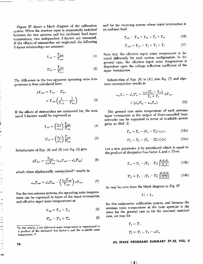
Figure 57 shows a block diagram of the calibration

system. When the receiver input is sequentially switched

between the two antenna and hot (ambient) load input

terminations, two independent Y-factors are measured.

If the effects of mismatches are neglected, the following

Y-factor relationships are assumed:

Topif

Y..t- Topa (1)

Y.'I,,- TopicT'o,,., (2)

The difference in the two apparent operating noise tem-

peratures is then calculated from

.aTol,._ = Tova -- T'os,_l

If the effects of mismatches are accounted for, the mea-

sured Y-factors would be expressed as

y,,= (a,h_ To,,h• ,,.,ol _ (4)

r';" -- \.,,,/T% (5)

Substitutions of Eqs. (4) and (5) into Eq. (3) give

_ To.. (,r,_To..-a_T'_) (6)_Tov<, alhTovl,

which when algebraically manipulated _'_results in

-- ' T' ( a,hTovh _aiaTova -- aia ova -_ ATovA (7)\ Top_ t

For the two antenna systems, the operating noise tempera-

tures can be expressed in terms of the input termination

and effective input noise temperatures as

Toga = Tia + Te_ (8)

T'ovo = T_ + T',, (9)

'qn this article, a net delivered noise temperature is represented as

a product of the mismatch loss factor a and the available noise

temperature T.

and for the receiving system whose input termination isan ambient load

Tov_ = T_h + Teh = Tp + T.s (10)

T<,r,,,= Tilt -_- T< = T,, + T< (11)

Note that the effective input noise temperature is de-

noted differently for each system configuration. In the

general case, the effective input noise temperature is

dependent upon the voltage reflection coeflqcient of theinput termination.

Substitution of Eqs. (8) to (11) into Eq. (7) and alge-

braic manipulation results in

"_h [Tp + T_,,]= triaTia + T v + Te "

o:iaTia # ' ATov i

+ [.,_T'_- re.T<.] (12)

The general case noise temperature of each antenna

input termination at the output of three-cascaded lossy

networks can be expressed in terms of available power

gains as (Ref. 2)

Tia = Tr - (T_, - T,,) r,r2r:, (13a)

T _ = Tv (Tv 2r*_) ' ' '__ -- T1T2T, _ltl(14a)

Let a new parameter fl be introduced which is equal to

the product of dissipative loss factor L and r. Then

T,, = T v - (T n -- T.) fl,fl_fl3 (13b)L,L2L_

# •1_3

T_ = Tp - (r_ - T'_) L'L'L" (14b)1 2 3

As may be seen from the block diagram in Fig. 57

L# a : L._

for this radiometric calibration system, and because the

antenna noise temperature at the horn aperture is the

same for the general case as for the assumed matched

case, we may let

ZlI _ TA

2_= T,_ = TA -- ATA


I ti

Tih = Tp

AMBIENT LOAD

INPUT TERMINATION

HORN

APERTURE

ITa -_ Z01

EXTERNAL

ENVIRONMENT

(SKY, GROUND,AND COSMIC

RADIATION)

7

(r2b)l "_ (F2b)2 "_

I1

[B1] z_ [B2]l

1L 1' Tp j L2, Tp

._j_ FEED COMPONENTSq_-----CONICAL HORN WITH UNKNOWN

LOSS L2

IiI

Z03

I

II

÷ANTENNA INPUT TERMINATION IN NORMAL WAVEGUIDE CONFIGURATION

[B3 ]

L3, Tp

WAVEGUIDESECTION

Jgl

T' ---i_a

F'a -: Fa "_ (F2b)i "_

I I

EXTERNAL

ENVIRO NME NT

II

II41--_- CONICAL HORN --_

LI , Tp

[B_]

L_, Tp

SUBSTITUTEDWAVEGUIDE

SECTION WITH

I

L3, Tp

._j___ WAVEGUIDE __

SECTION

KNOWN LOSS L_

ANTENNA INPUT TERMINATION IN SUBSTITUTED WAVEGUIDE CONFIGURATION

Fig. 57. Block diagram of radiometric loss calibration system

RECEIVER INPUTREFERENCE PORT

IF;h _1_

I__¢

II1

rla ._-_ Fr

I.LT

Z0R

iT

II

--'1

1

I--t____J

I

RECEIVER

JPL SPACE PROGRAMS SUMMARY 37-$2, VOL. II 75

Substitution of these values into Eqs. (13b) and (14b) gives

T,_ = Tp - (Tp -- Tit) fllf12/_3LILzL3

(13c)

g p

Ti_ = Tp - (Tp - Ta + _T,,) r'L'L (14c)

and final substitutions of Eqs. (13c) and (14c) into Eq. (12)

and solving for L:_,1 results in the expression

1 _ fl_/5'/3_a_ '_ (_) (1 + _XT,

- Tp - Tail "ij' \Tp + T_ )l AT°p4"

(15)

The dissipative attenuation of the line section having theunknown loss is then calculated from

A, = 10 log_o L._, (16)

Expressions for the a's and fl's are tabulated in Table 11,

and expressions for effective input noise temperatures are

given as

Te h --

×[(1[rihj2 } (17)

Tect (1-aJF,[_) { /'_,_lr,_[ 2 ),,_ T_o + \1 -- Ir,ol _ T, + 2r,°lr,o I

_ ir,ol _] ,o _ (is)

Trea -_,o lr_ol _ "y,ol ,ol

I( ?t× i --_1 T,oT, (19)

In the above, the effective input noise temperatures are

written in terms of a direct wave component T_o and

reflected wave eomponent. As was pointed out in Ref. 2,

expressions of this type are useful when noise propertiesof the individual networks in the overall receiver are

not known.

For the matched ease

(1) All a's and fl's become unity (Table 11)

(2) T_ = T_o = T_h = T_ = T'ea

and Eq. (15) becomes

1 L_[ aTA--(L'_L_L:,)ATopA]-- LiL" 1 + _-TZ-_a (20)

For small losses

F rLIL._L:, _ 1

so for the actual or assumed matched cases, the dissipa-

tive attenuation may be calculated from

Table 11. Equations for mismatch-related parameters

Parameter symbol Equation

B_

o- Ir,_PIo -lr, l_I1-r,_r,l'

c_-lr!.l'lc_- Ir, l')11- r,or,.l'

0 -lr.l') 0 - ls,,t,_l * - Irol lS.),]' 0 - [r,, I?)

0 -Ir,,I,'lO -Ib,,I/I[ I -- IF,hi, (b,,h ]' II -- lr,_ l,_)

p- Ir,.I,') 0 -Ib,,l.')I_-lr,_b(b,,)W0- Ir,,l'_

I_-Irol_0 -Ib,,l,'_0- I_,,I,'!0-Ib,,I.'_0- Ir_l'_[ [I -- (P,I (b,sh] [I -- IF,O, (bnh] [1 -- (U,_b lira,l,] [1 -- ¢,_P,] t_

NOTE: Equations for a_[a, _, fl_, and _ can be obtained by priming the reflection ¢oefflclent symbols in the corresl_.ndlnll _luatlons above. However, the Ua, (b_n).% and

Fr symbols need not be primed, since for this radlometric system, I a _ l'a, (bn)s -- (b_)z, and l_r _ Ft.

76 JPL SPACE PROGRAMS SUMMARY 37-$2, VOL. II

10log,. /' 10 lo_g,oe+ (ATo_a ATA)\ T,, - r,, /

m

(21)

The horn loss factors 1,1 and L_ do not necessarily have

the same value, because different waveguide modes can

be propagating in the horn when the system is in the

normal and substituted feed configurations.

d. Mismatch error analysis. The actual value of As can

be calculated directly from Eq. (16) if phase angles andcorrelation coefficient values are known. Note that .in

Table 11, the mismatch-related parameters contain factors

of the form I 1 - F,r,, l _which can be expressed as

Table 12. S-Band ultra cone input data

for computer program

Ambient load input termination

T_ --_Tp _ 305.9"K

Ir,_l = 0.003

Antenna Input termination in normal waveguide configuration"

T, _- TA ---- 5.410K

lr.I _ o.o

Ib,1f_ = 0.002

! b,a I = _ 0.020

I bt, 13 --_ 0.009

A] ---- 10 Iog_oLl ---- 0.0042 dB

Aa _- IOIog,oL= ---- 0.0200 dB

I r=b [t = 0.002

Ir,_l: = o.oi6

ir,.I = o.oo6

Antenna input termination in substituted wavegulde configuration

[r'l = Ir.l_o.o

Ib;,I, -- 0.002

Ib',,l, = 0.OO8

Ib',l, = Ib-1,

A't ---- 10 lag_oL'a---- 0.0034 dB

A': ---- 10 Iog_oL_-----0.0058 dB

A' = A,

Ir;_ J, = 0.002

Ir;bl, -- o.olo

Ir',,l -- o.ols

Common system parameters

Tp z 305.9"K

T, ---- 5*K

_,Ta ---- --0.37"K

ATop., = --0.234"K

T_,_ T_ ---- 50K

T_ = IO*K

Ir,l= o.loo

aSlnce part1 of thls system support prol_gation of circular polarization and two

wavegulde modes, effective reflection coefficient values wore used for Ibllll,

1_,1=, Ir,_l,, and It,hi,.

I1-r.r,,l = 1-21r=llrv Ieos( = + lr.l:lr.,l

(22)

where ,I,. and _ are, respectively, the phase angles of

1_ and r_. However, if only the magnitudes of r= and r,,

have been measured, then I1 - r,r_,l _ would be an un-

certainty which has limits of (1 ___Ir llr l) Another"

uncertainty in radiometric calibrations is usually the cor-

relation coefficient _, which has limits of ± 1.

For the present error analysis, peak mismatch errorswill be defined as the differences between the value of A_

obtained from Eq. (21) for the assumed matched case and

the maximum and minimum possible values obtained for

the actual mismatched case. Because many uncertainties

are involved in the radiometric calibration technique, it is

diJ]qcult to derive general case expressions for the error

limits. However, a numerical solution was readily ob-

tained when Eq. (16) was programmed for the IBM 1620

computer. In this program, the phases of reflection coeffi-

cients (involved in the uncertainty factors) and magni-

tudes of correlation coefficients are stepped through their

range of values in differefit possible combinations. Each

new computed value of A_ is checked against the previ-

ously computed value, and in this manner the maximumand minimum value of As can be found.

Table 12 is a tabulation of computer program input

data applicable to the S-band ultra cone. Using these

input data, the computer determined the maximum and

minimum possible values of A: to be 0.012 and - 0.004 dB,

respectively, for the most unfavorable correlated case. For

the uncorrelated (_ = 0) case, the maximum and mini-

mum possible values of A= were found to be 0.007 and

0.001 dB, respectively. These values of As may be com-

pared to the apparent Az value of 0.007 dB obtained when

neglecting the effect of mismatches. Since the results of

the uncorrelated case are believed to be the most likely,

the largest mismatch error is

EA2/ml_mateh = (A._).pp.... t - (A_),,,,

= 0.007 - 0.001 = 0.006 dB

References

I. Computer Programs for Antenna Feed System Destgn andAnalysis: Volume I. Programs and Sample Cases, TechnicalReport 32-979. Edited by A. Ludwig. Jet Propulsion Laboratory,Pasadena, Calif., Apr. 15, 1967, pp. 143-158.

2. Otoshi, T. Y., "The Effect of Mismatched Components on Micro-wave Noise Temperature Calibrations, IEEE Special Issue onNoise, to be published September 1968.


5.WaveguideFlangeSealLossMeasurements,C. T. Ste|zried, D. L. Mullen, and J. C. Chavez

Waveguide transmission line losses are an importantconsideration in the design of the DSN low-noise receiv-

ing systems, The waveguide transmission line must also

be pressure-tight, since these systems are normally oper-

ated at about 5-oz positive pressure, using nitrogen gas.

These conditions are normally satisfied by the use of

special heavy hand-lapped flanges. Figure 58 shows a -_- ....

WR 430 waveguide assembly during hand lapping.

Under some conditions it might be advantageous to usea seal which reduces the flange flatness tolerance required.

A commercial WR 430 waveguide seal (5906-430-1) TM is

available that seems to meet these requirements (Fig. 59),.

The crosshatched effect on the inner surface provided by

precision chemical etching is used to decrease ohmic con-

tact resistance. The manufacturer's reported insertion lossdetermined from RF resistance measurements for this

seal is 0.00004 dB, which is their limit of measurement

reliability. Measurements have been made at JPL with

a sample seal using the dc potentiometer insertion loss

instrumentation (Ref. 1). The loss is measured to be less

than 0.00005 dB (the present instrumentation resolution)

at 2295 MHz which is in agreement with the above.

Although this loss for the seal is negligible for most

applications, hand lapping of waveguide components is

considered to be preferable for the research low-noise

l_Parker Seal Co., Culver City, Calif.

Fig. 59. Commercial WR 430 waveguide seal

receiving systems. The seal cannot compensate for flange

faces which deviate badly in flatness. Since the inside

edge of the seal is raised, there is also a greater danger

that improper assembly could result in nonuniform flange

contact. This problem has been largly eliminated by themanufacturer with the introduction of the series-2 model.

These units have an outer ridge on the flange face which

reduces misalignment.

Reference

1. Stelzried, C. T., Reid, M. S., and Petty, S. M., "A Precision DCPotentiometer Microwave Insertion Loss Test Set," IEEE Trans.Instrum. Meas., Vol. IM-15, No. 3, September 1966, p. 98.

6. Efficient Antenna Systems: X-Band Gain

Measurements, 210-ft-diam Antenna

System/_ l). A. Bathker

a. Introduction. Late in 1966 a listen-only X-band

cassegrain experimental (XCE) feedcone was constructed

for the purpose of evaluating radio-frequency perform-

ance of the DSN ground antennas. The feedcone is com-

patible with DSN 85- and 210-ft diam reflectors and has

been operated on the Venus DSS 85-ft diam antenna on

two occasions during 1966 and 1967. RF performance

of the 85-ft diam antenna system at X-band has been

reported, using both radio astronomical (SPS 37-49, Vol. II,

pp. 65-67) and independent ground-based techniques

Fig. 58. WR 430 wavegulde assembly

hand-lapping process_WMadewith assistance from Division 33 and Bendix Field Engi-neering teams at the Mars and Venus DSSs.


1:1!

(SPS 37-50, Vol. II, pp. 49-52)? _ In February 1968 theXCE feedcone was operated on the Mars DSS 210-ft diam

antenna, at 8448 MHz.

The RF optics efficiency prediction for the 210-ft diam

antenna system is reported here. Also, reflector surface

tolerance predictions, based on structural computationsand field measurements reported in Subsection D-l, are

included to yield an overall predicted system efficiency at

_A summary of all 85-ft reflector data will appear in Technical

Report 32-1300, Radio[requency Performance of an 85-# Diam-

eter Ground Antenna: X-Band, D. A. Bathker (in process).

the maser reference flange within the XCE feedcone. A

portion of the February 1968 RF tests is shown to comparepredicted with measured results.

b. Computed RF optics efficiency. The RF optics

_lqciency for the 210-ft diam antenna system at X-band

is predicted by inputting the primary feed pattern

(Fig. 60) and the subreflector configuration (Fig. 61) to

the Rusch Scattering Program (Ref. 1). The scattered pat-

terns shown in Figs. 62 and 63 illustrate slight distortion

occurring near the edge of the paraboloid (illumination

angle 50-60 deg) caused by the optimum S-band beam-

shaping fange. As in the case of the earlier 85-ft diam

-10

-20

.<

-30

-40-108 -36 0 36

ILLUMINATION ANGLE, deg

Fig. 60. Primary-feed radiation pattern, dual mode feed

72 108


-_ 18o30 '

_/_-132.000-;n. R

13°28_ 6 _ -120. O00-1n. R

570. 000 in.

_'--- HYPERBOLOID

Fig. 61. Subreflector configuration

o

m

8O

0

-10

-20 --

-30 -

-40 _V_ _ _-_

-10_

i

-72 -36 0 36


Fig. 62. Subreflector scattered radiation patterns, E- and H-plane amplitude

72 I 0_

JPL SPACE PROGRAMS SUMMARY 37-52, VOL. Ii

! II

reflector X-band evaluation, the removal of the S-band

flange was not warranted. The scattered patterns were

then evaluated with the JPL Antenna Efficiency Program

Table 13. Feed efficiency, XCE feedcone

Parameter Value, %

Forword spillover

Rear spillover

Illumination efficiency

Cross-polarization efficiency

Phase efficiency

Subreflector blocking efficiency

7,22

0.20

86.81

99.94

96.62

96.45

Overall feed efficiency 74.86 --4-0.20

(SPS 37-26, Vol. IV, pp. 200-208). Results of that study,

as they apply to the components under consideration, aresummarized in Table 13.

An optical analysis of the 210-ft diam antenna quadri-

pod shows that the structure blocks 6.255% of the availab]e

aperture. Assuming that tile percentage of intercepted

energy equals the percentage of area, which constitutes

accepting "pie-slice" approximations of the blocked areas

in the aperture, it has been shown

'= (1 - B) _

-o

uj_

<"l-ta_

wi--

5

180

90

-90

-180- 108 -72 -36 36 72 I0_


Fig. 63. Subreflector scattered radiation patterns, E- and H-plane phase


where _;'/_ is the blocking ea_ciency, and B is the frac-

tional area blocked (SPS 37-41, Vol. III, pp. 89--90). Actu-

ally B = (rA, where a is defined as an average RF opacity

and A is the optically blocked area. Because of the large

wavelength size of the quadripod cross section at X-band,

the opacity is estimated to be 0.8 < e < 1.2. Table 14 gives

the components considered and the overall quadripod

blockage efficiency, assuming the estimated opacities rep-resent 1-a limits.

The dissipative attenuation between the antenna refer-

ence flange and the maser reference flange was previously

measured as (0.150 ± 0.0018dB), 3 _. Estimates of turn-

stile junction and horn losses are 0.025 and 0.018 dB,

respectively. Table 15 gives the components considered

and the overall waveguide efficiency.

The final value for the RF optics efficiency of the

210-ft diam antenna system, when fed with the XCE

feedcone, may be obtained from Tables 13, 14, and 15 as

7., = 0.6292-+-0.024

where the tolerance quoted is an estimated 1-a value,exclusive of surface tolerance.

c. Computed sur[ace tolerance efficiency. In Subsec-

tion D-1 the 210-ft diam reflector computed surface dis-

tortion is considered as a function of elevation angle,

augmented with measured distortions for the primary

panels, subreflector panels, and setting tolerances (Item I,

Table 19 of above-mentioned article). Figure 64 shows

the relation between gain loss and surface tolerance for

a frequency of 8448 MHz according to the methods of

Ruze (Ref. 2).

Table 14. Quadripod efficiency

Parameter

Blocked area A

Opacity o"

Value, %

6.255

80-120

Quadripod blockage efficiency t/'/r/ 87.88 4- 2.4

Table 15. Wavegulde efficiency, XCE feedcane

Component Attenuation, dB

Antenna to maser flanges 0.t50 4- 0.002

Turnstile iunctlon 0.025 4- 0.025

Feedhorn 0.018 ± 0.018

Overall waveguide efficiency 95.65 4-0.22%

o_

0

>-UZ

Ui.i.LL.LU

lOO

90--

80--

70

60

50

4O

\\\

\\

\30

G/Go: oxp 2]FREQUENCY = 8448 MHz

20 \,o

0

0 0.02 0.04 0.06 0.06 0.10 0.12 0.14 0.16 0.180.20

SURFACE TOLERANCE e, in. rms

Fig. 64. Surface efficiency as a function of

surface tolerance

d. Computed overall system efficiency and gain.

Tab]e 16 shows the computed surface tolerance, surface

tolerance e_ciency, and computed overall system effi-

ciency and gain of the 210-ft antenna system when fedwith the XCE feedcone. Table 16 surface tolerances

quoted are representative of reasonable environmental

conditions. Environmenta] effects are beyond the scopeof this reporting. Approximately 0.2-dB dissipation losswithin the XCE feedcone is included.

Table 16. Computed system efficiency and gain

Elevation Surface Surface Overall system Systemangle, tolerance, tolerance gain,

dog In. rms efficiency, % efficiency, % dB

0

15

30

45

60

75

90

0.066

0.058

0.051

0.048

0.055

0.074

0.102

70.6

76.4

81.4

83.2

78.6

64.4

43.5

44.4

48.0

51.2

52.3

49.5

40.5

27.4

71 .S

71.9

72.2

72.3

72.0

7f.1

69.4


III

e. Measured overall system efficiency. As stated in

Subsection D-I, the computed total surface tolerance

figures (Item I, Table 19 of referenced article) are repre-

sentative of a paraboloid of changing focal length as a

function of elevation angle. Item D of the same table

gives the computed focal length change required to main-

tain optimum gain as observed on the control room indi-

cator, and the computed focal length change is plotted

in Fig. 65.

Figure 65 also shows RF data which were obtained by

maximizing receive system noise temperature on source,

using the hyperboloid axial drives. Focusing was the first

step taken in the February 1968 X-band evaluation. When

found repeatable for the source ascending and descending

in elevation angle, the data in Fig. 65 were used to

manually correct the antenna focus for all following data.

The source M84 (a spherical galaxy in Virgo) was selected

as a high elevation angle calibrator.

Figure 66 shows the efficiency measurements made

using four selected sources. The assumed source fluxdensities, distributions, and beam correction factors may

be inferred from the 1003 efflciency temperature quota-

tions given. As improved values of radio astronomical flux

become available, certain corrections may be possible.

For example, the Virgo (3C274) data appear consistently

low when compared with the Venus data. It is beyond

the scope of this reporting to study the flux tolerances.

All data are plotted as measured, i.e., the effect of

die atmosphere is included in the overall system cfiqciency

concept. A first-order estimate of atmospheric attenuation

at 10 deg elevation angle is 23 in terms of e_ciency. The

measured data are seen to fit the computations remark-

ably well. Measured data were obtained on a 24-h/day

basis, i.e., no attention was given to possible thermal

effects during the bright days. Similarly, no attention

was given to possible wind distortions; however, the

maximum wind velocity was always below 20 mph.

1.2

1.0

c

z"O

0.8.,(Uia

Z

6Iu 0.6z

0

o

_ 0.4

Z0u

0 1 20

/

)0 0 ,,,,.0_0

/

30 40 50

ELEVATION, deg

• 3C273 ASCENDING

O 3C273 DESCENDING

O MB4/", PREDICTED

BASED ON PARABOLOID

BEST FITTED TO STAIR-

COMPUTED DEFLECTIONS

7"

60 70 80 90

Fig. 65. Focus as a function of elevation angle


>-zu_l

U

l--

.a,

O

7o

65

60---

55

5O

45,--

4O

35

30

25

2O

&

S-BAND 58% AT

IPREDICTEDBASEDON:

APERTUREINTEGRATION 74.9%QUADRIPOD BLOCKING 87.9°/0DISSIPATION LOSSES 95.7°/0NET RFOPTICS EFFICIENCY 62.9%SURFACETOLERANCE AT 15°, 0. 058" rms, 76.4o/0SURFACETOLERANCE AT 45°, 0.048" n_s,83.2%SURFACETOLERANCE AT 75°, 0.074" rms,64.4°/0

L

O/,

MASER REFERENCE

a a o_O

_o a Om

o

0

0

A

Z_0

o

rO

O

OE3O

--A

O

¢o

¢

O

O&O0

Q o¢

O>

o0

0

0

kD [_ o

[] Oo

> ¢0

3C123 BASEDON 10.7°K FOR I00O/O_;3C274 BASEDON 46.4°K FOR 100%?3C405 BASEDON 140°K FOR 100%zlVENUS BASEDON 600°K BLACKBODYINCLUDES ATMOSPHEREWIND VELOCITY 20 mph (MAX)

o O

gO

I0 20 30 40 50 60

ELEVATION, deg

Fig. 66. Measured overall system efficiency at maser reference flange

70 80 90


I 111

lZD

oZ0 Z

U

-o

o

Z

i

Z

"r-l--

o

I

Z

_3MOd 3AIIV73_I

e-0

oi

o

0"0

u_

"6e-

U_

,0

U.


Because of the manual focnsing as a function of eleva-

tion angle, Fig. 66 represents the best performance pres-

ently available. The possibility that the measured surface

distortion (Table 18 in Subsection D-I) rather than the

computed (Table 19 in the same article) more nearly fits

the RF data above 60 deg elevation is apparent in Fig. 66.

This would indicate the surface tolerance may approxi-

mate 0.090 in. rms near zenith.

f. Conclusions. The February 1968 X-band RF tests onthe 210-ft diam antenna system have confirmed the

previous RF optics and structural deflection computa-tions. There is some evidence that the structural com-

putations near zenith may be conservative.

The system performance is seen to be very good, with

a peak system gain of 72.3 dB and a peak system effi-

ciency of 52,_. Scans of the quasar 3C273 at 35 deg ele-

vation angle confirm the expected narrow (0.038 deg)

beamwidth. Figure 67 shows declination and hour angle

scans, respectively, for this source which produced an

increase in system temperature of 25°K. Performance of

the pointing system was found to be excellent for thenarrow beamwidth for elevation angles above 20 deg.

Possible refinement of corrections for atmospheric refrac-

tion below 20 deg elevation may be necessary,

References

1. Ruseh, W. V. T., Scattering of a Spherical Wave by an Arbi-

trury Tr_mcated Sur[ace of Revolution, Technical Report 32-434.

Jet Propulsion Laboratory, Pasadena, Calif., May 1963.

2. Ruze, J., Phy._ical Limitations on Antennas, Technical Report

248. Research Laboratory of Electronics, Massachusetts Institute

of Technology, Cambridge, Mass., Oct. 1952. (See also John

Ruze, "Antenna Tolerance Theory-A Review," Proc. IEEE,

Vol. 54, No. 4, April 1966, pp. 633---640.)

D. Supporting Research and Technology

1. Primary Reflector Analysis (210-ft-dlam Antenna),M. S. Katow

a. Introduction. This article describes the methods

used to analytically compute the distortions of the 210-ft-diam antenna's reflector structure under gravity loadings.

The deflections were output from the STAIR structural

computing program (Refs. 1 and 2), and the distortions

were evaluated by the rms of the residuals after best fit-

ting by a paraboloid using the RMS program (SPS 37-40,

Vol. IV, p. 176 and Ref. 3).

Comparisons were made to field-measured results interms of the rms of the distortions and by the computer-

organized contour plots of the residuals.

86

Finally, the total distortion of the RF pathlengths due

to the primary reflector surface errors was added to thesubreflector surface errors and to the equivalent rms

error due to its lateral offsets for every I5 deg in eleva-

tion angle. All surface panels were set and aligned with

the primary reflector positioned at an elevation angle of

45 deg.

In Chapter III-C-6, D. Bathker presents the resultsof X-band field tests on the 210-ft-diam antenna. Those

results are compared with the final total distortionsherein.

Since the best-fitting paraboloid included the focal

length as a parameter in the fitting process, the re-

focussing was accomplished in the field test by trans-

lating the subreflector in the axial direction at each

elevation angle. In normal S-band operations, refocussingis not done since the somewhat larger effective rms at the

extremes of the elevation angles results in minor loss in

efficiency.

b. Formulation of the structure. The input-data size

limitations of the STAIR program limited the structural

input to only one quadrant because of the followingfactors:

(1) The gravity loading data could only be directly

generated within the size limitations and com-

puted with minor changes of the coding, lr

(2) At least three loading conditions could be com-

puted per run.

(3) The data card count was already large (about

6000).

(4) Each computer run required ll& h initially (now

reduced to 50 min).

(5) The low-use experience of applied computer an-

alysis to antenna design did not justify the addi-tional cost and difficulties of a l_-section analysis.

Since the elevation wheel truss portion of the reflector

structure assembly was only truly symmetric about one

plane, the need arose to consider the lh section of data.

The nonsymmetry about the other plane resulted from

the open section required between the two elevation

gears for rotational clearance to the optical tower, locatedon the azimuth axis. Thus, the structural functions of

these removed cross bracings needed to be assessed as to

their effect on the deflections due to gravity loadings.

'_This limitation was increased to 1200 total joints in Ref. 2.


Iil

Considering that the main trusses which are most effec-

tive in reducing deflections were in-plane and consider-

ing the negligible effects of the cross-bracings which are

required mainly as restraints against the torsional forcesor movements between the elevation wheels, it was de-

.cided that the assumed symmetry of one quadrant data

would adequately represent the complete structure.

With one (first) quadrant of data, the computations

for gravity load deflections required two separate com-

puter runs, one with symmetric restraints on the joints

in the boundary planes and the other with antisymmetrierestraints on the joints. By use of restraints on the joints

in the boundary planes satisfying the equations of con-

dition noted in Ref. 4 and shown in Figs. 68 and 69

for the symmetric and antisymmetric |oadings, respec-

tively, the deflections for the gravity "off-on" or 1.0-g

loads were computed.

Since the gravity vector in practice changes only in its

direction to the symmetric axis of the reflector structure,

the deflections from the setting position (45-deg eleva-

tion angle) of the surface panels were easily computed

by resolving the gravity vector into two components,

the one component parallel and the other normal to the

symmetric axis of the reflector structure. As shown in

Fig. 70, the deflections at zenith look are the sum of

the changes in the above described components. The

symmetric load component increased from 0.7 to 1.0 g,

and the antisymmetric load component decreased to 0

from 0.7 g.

The deflections from the symmetric and the anti-

symmetric loading cases were actually added in the

paraboloid best-fitting computer program (Ref. 8). Therms of the residual distortions, as well as the parameters

of the best-fitting paraboloid, were output. The program

also produced, using the SC 4020 plotter connected tothe IBM 7094 computer, a contour level map of the re-

sidual distortions in terms of ½-RF pathlength errors

after best fitting.

c. Results. The results for the STAIR-computed cases

for the horizon look (0 deg) and zenith look (90 deg),

with the surface panels set to "perfect" paraboloid at

45-deg elevation angle, are shown on the left-hand sides

of Figs. 71 and 72. These contour level patterns were

duplicated as produced by the plotter except for the

enlarged numbers that show the values of the contour

levels and the increased-width zero (0.0) level lines. The

rms values in Figs. 71 and 72 refer only to the panel

support points in the reflector structure.

The technique used for the field readings is illustrated

in Fig. 78. Using as the geometric base the arc length

from a strap gage that was used to drill the panels for

the target placement holes and the computed instrument

angle O, the surface panels were adjusted to a paraboloid

shape, and the target readings were also used to measure

the deflection under the gravity loadings. The readings

were continuously measured and checked with respect

to a four-target datum reference plane at all elevation

angles. After best fitting, the results are shown on the

right-hand sides of Figs. 71 and 72.

The distortion vectors in the field data contour charts

were all assumed to be normal to the line of sight as

read by the theodolite, and conversions to vectors par-

allel to the symmetric axis of the paraboloid were made

by dividing the readings by the cosine of the instrument

angles. Although it is possible to compute the direction

of the deflection vectors from the STAIR program as afirst-order correction to obtain a more conservative re-

sult, the data was best-fitted after it was assumed that

the measured deflection vectors were parallel to the

normals to the paraboloid. The new values wererms = 0.068 in. for the zenith-look ease and rms = 0.084

in. for the horizon-look ease.

To establish the rms distortion values compatible for

RF performance calculations, it was necessary to com-

pute the surface distortion at a 45-deg-elevation panel-

setting position and add it to the distortions caused by

the gravity loading at the zenith- and horizon-look posi-

tions as a change from the 45-deg position. For the

45-deg elevation setting position, the rms distortion of

the surface-panel setting error was added as a random

error to (1) the surface-panel manufacturing error, and

(2) the subreflector manufacturing error. Since all align-

ment of the surface panels was done for the 45-deg

position, no error was assigned for any misalignment.

Table 17 gives the measured surface distortion at a

45-deg elevation angle.

Table 17. Measured surface distortion of 210-ft-diam

antenna at 45-deg elevation angle

Error source Error, in.rms

Surface-panel setting

Primary surface-panel manufacturing

Subreflector manufacturing

Total 1/2-RF-pathlength error

0.019

0.035

0.027

0.048

JPL SPACE PROGRAMS SUMMARY 37-52, VOL. !! 87

II!I

-x ---4-

I

|

I

f/

/

/

/

/

/

//

\

I

I

II

-- X.._J-i

,%

\

\

\

\

\

+y

----- LoAo" © r- © TYPICAtJOINTI V/--X_ y_ ELEVATION

/ / / _1 _, _///////_/ _ I V / / _ _ I _ (_) ELEVAT IO N

,_-r-I ' [ +x +_ ---

,, ,,_,\ ,--

" ]k I / I ).,

/ i I // _--- TYPICAL RESTRAINT

I // I //"" "/ /

-y

PLAN VIEW SIDE ELEVATION

Fig. 68. Symmetric loading--boundary restraints for first quadrant data

i/

//

/

/

/

/

t

\\

\\

\

\

1.0-g LOAD

+X +z

/

"" ® i """© TYPICAL JOINT IN

- - .... _ BOUNDARY PLANE

-y ®= Z RESTRAINT

PLAN viEW

[_ /-_ ® ELEVATION

GEAR PINION

I i ,," _ TYPICALY RESTRAINTI /

I /I /

I /I /

I /I /

l /l

SIDE ELEVATION

Fig. 69. Antisymmetrlc Ioadlng--boundary restraints for first quadrant data


1|1_

_.o.zg(HoRIzoN_\ .,d_ , 1.0g/ZENnHI

,_-0.7 g (ZENITH)

,,_ _1.0 a _ GRAVITY LOAD AT ZENITH/",,t/ _-,.u _ LOOK= 0.3(ZENITH)

/ _.__ -0.7(HOR,ZON)I / _iv _ --- - PERFECT PARABOLOID

"! _5 :_g_ SET AT 45-deg ELEVAT,ON

V_I. 0 g u__ GRAVITY LOAD AT HORIZON LOOK• (HORIZON) = -0.7 (ZENITH) +0.3 (HORIZON)

Fig. 70. Gravity loading diagram for deflection

computation

(o) (b)

O6

+0.03

+0.06

RMS: 0.040 in.FOCAL LENGTH CHANGE: -0.69 in.

Fig. 71.

-0.06

0

RMS: 0.032 in.FOCAL LENGTH CHANGE: -0.52 in.

Horizon-look contour maps of 1/2-RF-pathlength errors: (a) computed, (b) field reading after best fit


(a) (b)

10 10

00

10 -0.10

+0.10

+0.10

RMS: 0.075 in. RMS: 0.057 in.

FOCAL LENGTH CHANGE: +0.29 in. FOCAL LENGTH CHANGE: +0.181n.

Fig. 72. Zenith-look contour maps of 1/2-RF-pathlength errors: (a) computed, (b) field reading after best fit

iHILGER-WATTS

ALL ATTITUDE

THEODOLITE

VERTEX

3RAIN

FEED CONE

MEASUREMENTINSTRUMENT SECTION _ REFLECTOR SURFACE

90 deg

THEODOLITE

ADAPTER

15 in.

DATUM

REFERENCE

e INSTRUMENT

ANGLE

;ETS

STRAP GAGE

BRIDGE TOOL

Fig. 73. Surface measuring technique

i


I111

For the horizon-look and the zenith-look positions of

the primary reflector, distortions in addition to those of

the 45-deg position are: (1) the reflector structure gravity

deflections of the surface panels' supporting points, and

(2) the equivalent rms distortion from the lateral and

axial offsets of the subreflector. These equivalent rms

errors are read from Fig. 74, whose values were cam-

Table 18. Measured surface distortion of 210-ft-diam

antenna at O- and 90-deg elevation angle

Source

45-deg elevation 1/=.RF.pathrength error

Reflector structure gravity deflections

from 45-deg elevation

Subreflector lateral offset

Total T/_.RF.pathlength error

Error, in. rnls

0 deg J 90 degm

0.048

0,034 0.063

0.020 0.050

0.062 0.094

puted by the Radiation programs (Ref. 5). Table 18 givesthe field-measured results and Table 19 gives the com-

puted results.

References

1. STAIR (Structural Analysis Interpretive Routine), Lincoln Man-

ual No. 48. Lincoln Laboratory, Massachusetts Institute of Tech-

nology, Lexington, Mass., July 1962.

2. Katow, M. S., Bartos, K. P., Matsumoto, R., IPL Modified STAIR

System-Operating Procedures, Technical Memorandum 33-804.

Jet Propulsion Laboratory, Pasadena, Calif., June 1, 1968.

8. Katow, M. S., and Schmele, L., Utkn-Schmele Paraboloid RMS

Best-Fit Program, in Technical Report 32-979, Vols. I and II,

p. 75. Edited by A. Ludwig. Jet Propulsion Laboratory, Pasa-

dena, Calif., April 15, 1967.

4. Newell, J. S., "The Use of Symmetric and Anti-Symmetric Load-

ings," 1. Aeronaut. Sci., p. 285, 1939.

5. Bathker, D., Radiation Pattern Programs, in Technical Report

32-979, Vols. I and II, p. 107. Edited by A. Ludwig. Jet Propul-

sion Laboratory, Pasadena, Calif., April 15, 1967.

Table 19. Computed surface distortion of 210-ft-dlam antenna from

change in direction of gravity vector from 45-deg elevation

Source

Best-flt parabolold data

Vertex y-coordlnate, in.

Vertex z-coordlnate, in.

Rotation x-axls, rod

Focal length change, in.

Quadrlpod apex z-deflectlon, in.

Subreflector

z-deflectlon, in.

Subreflector

axial indicated position, in.

Subreflector

lateral y-dlrectlon deflection, in.

Subreflector

lateral offset equivalent error, in. rrns

axial offset equivalent error, in. rms

Best-flt paraboloid reflector structure

distortion from 45-deg, in. rms

45-deg 1/=-RF-pathlength, in. rms

Total I/z -RF-pathlength-focussed axially

distortlon, in. rms

Total 1/=-RF-pathlength-focussed only at

45 deg distortion, in. rms

1.588

0.070

0.001015

-- 0.693

-- 0.025

--0.048

--0.77

--1.1

0.019

0.058

0.040

0.065

0.085

I5

1.403

0,044

0.000894

-- 0.439

--0.015

--0.028

-- 0.48

0.5

0.008

0.036

0.032

0.058

0.068

Etevation angle, deg

3O

0.806

0.021

0.000548

--0.203

-- 0.009

--0.017

--0.22

0.1

0.001

0.017

0.018

45 60

0.0 --i.121

0.0 -- 0.016

0.0 --0.000712

0.0 0.156

0.0 0.004

0.0 0.004

0.0 0.16

0.0 0.9

0.0 0.015

0.0 0.012

0.0 0.023

0.048

(Field measured distortion used for 45-deg position)

0.051

0.054

0.048

0.048

0.055

0.057

75

-- 2.426

--0.026

-- 0.001539

0.253

0.007

0.007

0.27

1.8

0.031

0.020

0.048

0.075

0.077

9O

--3.829

--0.029

--0.002427

0.285

0.010

0.010

0.31

2.8

0.050

0.023

0.075

0.102

0.105


0.080 /

u J"

U

8

I,-

zoI--

l,--

,,z.

O.070 /

O.060 -- /

/

0.050 - LAT7

/O.040

o. 030

O.020

O.OlO

0 1 2 3

SHIFT(RFFEEDOFFSETFROMFOCUSPOINT), in.

Fig. 74. Rms (equivalent) vs feed point axial andlateral shifts for 210-ft-diam antenna

2. Antenna Structure Joint Integrity Study (Phase Ill,V. Lobb and F. Stoller

a. Introduction. Experience with antenna structures

constructed of galvanized members has shown that their

connections have a tendency to slip under long duration

loading. In these structures where deflection is a failure

criteria, this slip at connections is a serious problem. Slip

in galvanized joints has resulted in distortion of the re-

flector parabola and in tolerance degradation in other

components of the antenna. A prime problem has been

the loss of gear running clearance between the pinion

92

and bull gear for both declination and hour angle mo-

tion. These antennas are subjected to varying conditions

for a large moveable structure, such as drive and wind

vibration, rapidly varying dynamic loading, load reversal,and sustained loads.

So that a means of eliminating this problem could be

devised, a joint integrity study was started. Phase I is a

five-part bolt testing program currently in progress, the

first two parts of which have been reported in SPS 87-47,

Vol. II, pp. 135-188 and SPS 87-50, Vol. II, pp. 177-179,

respectively. Phase II is a bolted-joint study which con-

sists of a thorough testing of bolted structural assemblies

exposed to long-term static shear stress, long-term static

shear stress with a superimposed transverse vibration,

and short-term static shear stress with repetitive load

reversals. This research program studied the effect of

such variables as joint and fastener coatings, bolt design

and strength level, shear and tension stress, and balanced

design tension-shear ratio. Tests and parts of the data

resolution were performed at a subcontractor's facility.

The economics of fabricating and maintaining structural

members exposed to weathering in isolated locations

require the use of corrosion-resistant protective coatings.

While coatings on faying surfaces are known to have

definite effects on joint performance under short-term

loading, no specific information has been available as to

how they contribute to joint behavior over a prolonged

period of time.

The study of time-dependent-slip in bolted assemblies

represents a new area of consideration in the field of

mechanically fastened connections. The results are of gen-

eral interest because of the importance of dimensional

integrity in various types of connections. Reduced test

results of the Phase II activity are presented in this

article. A future JPL Technical Memorandum will present

the specifications, test data, apparatus description, etc.

b. Test results. Tests were made of 110 bolted joints.

The joints, consisting of A86 steel plates and angles,

were fastened with high-strength bearing bolts and hex

head bolts in ASTM A825 and A490 strength grades; s

Both the high-strength bearing bolts and hex head bolts

were used to assemble friction-type and bearing-type

joints.

The steady-state slip behavior of structural connectionstested in series A and B followed the general patterns

schematically illustrated in Fig. 75. Curve A represents

the behavior of bolts with very poor slip resistance. The

1"ASTM = American Society for Testing Materials.


11!

,D-

ttl

FULLBEARING

f A

I_- c

0 48

TIME, clays

Fig. 75. Typical joint slip curves (series A and B)

relative joint movement was rapid, being restrained only

when complete bearing was achieved. Curve B is repre-

sentative of the behavior of most highly loaded friction

connections. Joint extension was noticeable immediately

after loading, but after a relatively short period of time

steady behavior occurred. Curve C is typical of bolted

connections with good slip resistance. After initial ex-

tension, a very low slip rate or a zero slip rate wasobserved.

Typical examples of the three curves and their physical

properties are as follows (laying surface coating gen-

erally affected the joints' slip resistance): curve-A-type

joint slip occurred on a red-oxide-painted surface;

curve-B-type joint slip occurred on galvanized and red-

oxide-painted surfaces; curve-C-type joint slip occurred

on mill-scale and inorganic zinc-painted surfaces.

The joint deformation that occurred in the series C

load reversal tests for mill-scale laying surface is illus-

trated in Fig. 76. Several of these tests demonstrated

the same behavior under sustained load as was experi-

enced in series A and B, and this is evidenced by the

positive or negative slope of the curve during the 2-h

period. These specimens were not assembled in bearing

so that, when the load was reversed, the joint deforma-

tion returned to zero and then became negative. After

unloading, in either tension or compression, considerable

recovery of the joint deformation occurred.

The results of series C stress reversal tests on inorganic

zinc-silicate laying surfaces were radically different thanthe data generated in the series A and series B tests.

Although the general relations between joint slip and bolt-

type or joint slip and shear stress appear to be approxi-

mately the same, the maximum deflections are quite

inconsistent with the data on the effect of laying surface

condition. Under a condition of stress reversal, the

o. 004[ T

z 0 L lEST250 z0.002

._o,

19, 400-1b LOAD

T T T T T T [ r

Z

oLUU<

r_ Zoo_ z- o. oo2

oU

- O. 004

c!

II I I I I I I I I I2 4 6 B 10 12 14 16 18 20

TIME, h

Fig. 76. Deflection time graph for mill-scale laying surface


inorganic-zinc coating breaks down and frets away, caus-

ing a reduction of bolt preload, which allows increased

joint slip. This breakdown is shown on the deflection

time graph (Fig. 77). The peak deflection occurs after

several cycles and is four times that of a mill-scale layingsurface.

Figure 78, the graph for galvanized laying surfaces,shows a definite variation in the deflection behavior of

the galvanized joints after cyclic loading. After several

cycles of load reversal, these joints showed a tendency

to "lock up" or cold weld so as to reduce the amount ofdeflection occurring. However, these deflections still were

greater by a factor of two than joints with mill-scale

laying surfaces. Furthermore, under sustained load, the

slope of the deflection curves was unaffected by thisfactor.

Joint slip data of series A, B, and C show no signifi-cant effect of bolt finish on slip performance. Several

otherwise identical joint pairs, except for having gal-

vanized, mechanical zinc-coated, and inorganic zinc-

painted fasteners, show no repeatable difference in joint

slip. None of the three protective finishes provides a

substantial advantage over the others.

The effect on joint slip caused by adding a transverse

vibration to the joints (series B) was little at stresses

below i0,000 lb/in. 2 Above that level, the total joint slip

in high-strength hex head bolts was increased consid-

erably by the addition of vibration, but for the high-

strength bearing bolt (HSBB) there was no effect on the

total joint slip. However, the addition of vibration had

little or no effect for either type of bolt on the slip

rate (in./h).

When bearing bolts are used, faying surface coatings,

such as paint and galvanize, create no change in fatigue

life over a mill-scale laying surface. In service conditions

requiring friction-type joints, two high-strength bearing

__o

z

U

rn

94

O. 010

O.008

0. 006

0. 004

0.002

Z

_o0u

- 0.004

I I I

TEST 33

19, 400-1b LOAD

/

....,--"""1 1

i

Ll_m

f" _"_1I

I

I I 1

0 2 4 6 8

'rJ

I i

1 I I i

!F _ _ -'1 ¸I

r

i

I

1 110 12

TIME, h

I I I14 16 18 2u

Fig. 77. Deflection time graph for Inorganic zinc-silicate faying surface


II!!¸

o.0o6 T T T T T T T T T

O.002

0

TEST 27

19, 400-1b LOAD

2 4 6 8 10 12 14

TIME, h

-LOCKING UP

INDICATED BY

DECREASE 1NTOTAL JOINT

MOVEMENT

16 18 20

Fig. 78. Deflection time graph for hot-dip galvanize faying surface

bolts can be substituted for three hex head bolts without

causing any change in the time-dependent slip behavior

of the joint.

Figure 79 is a graph of nominal bolt shear stress versus

the logarithm of the joint slip under load (_) for the

galvanized joints in series A and B. On this semilog plot,

the value of ± increases in approximately a direct pro-

portion to the shear stress although the rate of increase

is considerably lower for the high-strength bearing boltthan it is for the hex head bolts. At shear stresses below

11,000 lb/in.% the average /x is quite similar for either

type of bolt (approximately 0.001 in.). Above 11,000 lb/in?

there is greater divergence, but at any given stress level

the high-strength bearing bolt has considerably less totalslip than does the hex head bolt.

In the high-strength bearing bolted joints, there is

relatively little difference in the magnitude of A at thevarious stress levels. There are two factors that allow

slip with these types of bolts: (1) a reduction in theamount of interference due to variations in hole size, and

(2) elongation of the bolt hole under load. Thus, the

general trend for the high-strength bearing bolted joints

follows closely the general trend of hole elongation

(shown in approximation).

hand, attempts (Fig. 80) to relate the time-dependent

slip factors with member tension stress were not as suc-

cessful. There is a qualitative relation between joint slip

and tension stress, but there is considerable scatter and

overlap in the data. The reason for this is that, with

changing tension-shear ratios, several shear stresses can

occur in any given tension stress range. Since slip be-

havior is more closely related to shear stress, comparisonsbased on tension stress are inconsistent.

The highest high-strength bearing bolt slip rate (in./h)

value recorded was only 4.86 × 10 -a. Thus, at the higher

stress allowed for bearing-type joints (22,000 lb/in. _ with

A825 bolts and 32,000 ]b/in7 with A490 bolts), and

regardless of faying surface condition, the high-strengthbearing bolt provides a slip rate lower than or equal to

that considered acceptable for friction-type joints under

current practice.

At stresses below 15,000 lb/in. 2, the laying surface

condition had no effect on total slip in the high-strength

bearing bolted joints. In high-strength bearing bolted

joints (static stress or unidirectional loading stressed

above 15,000 lb/in.2), galvanized surfaces caused some-

what more slip than did other types of laying surfaces.

The most significant influence on joint slip behavior

was the bolt shear stress level (Fig. 79). On the other

The most significant effect of faying surface condition

on joint slip occurred in the joints fastened with hex


a._Jt_

I--Z

O

100 J-_ ! T--

J BOLT

j HSBB

J HEX HEAD

I10 -I __-- rvl.L nLff_li_

T 1 r "r--

STAT IC V I BRAT I O N

A325 A490 A325

O _ C,

O _ O

V/

c / e

10 -2 O'_ ...... / HSBB_ i

HEX HEAD ,, .f./ c, ON

o/ IO -O

I HOLE ELONGATIONf (UPPER BOUND: TIS = I : 0.75)

10-4 / I ] I I

0 5 10 15 20 25 30 35

NOMINAL SHEAR STRESS, klb,/in. 2

Fig. 79. Joint slip vs shear stress

(series A and B galvanized)

head bolts. In order of increasing slip resistance (for

hex head joints under static stress or unidirectional load-

ing), these were: galvanized laying surfaces, red-oxide

primer-painted and plain mill-scale laying surfaces, and

inorganic zinc-painted laying surfaces. On reviewing the

uncorrected joint deformations, it became apparent that

the red-oxide primer joints experienced high deformation

on application of the test load. In this respect, the order

of increasing slip resistance would be: red-oxide-primer-

painted laying surfaces, galvanized laying surfaces, plainmill-scale laying surfaces, and inorganic zinc-painted

laying surfaces.

Staggering the direction of bolt insertion did not

affect the performance of the high-strength bearing bolt

joints. In the case of interference-type bolts, slip due to

plating occurs only relative to the general trend of hole

elongation if such occurs and if an interference or bear-

ing joint is actually achieved.

Bolts (ASTM A925 and A490 class) coated with in-

organic zinc silicate or mechanical zinc plating required

96

"u

ZOI-'-

klJ

O

0.14 --

0.12

0.10

0.08

0.06

0.04

0.02

I I IALL SERIES A SPECIMENS

ALL FAYING SURFACES GALVANIZED

I b IA325 HSBB O

A325 HEX HEAD Oi

9GO

I0

i

15 20 25

NET TENSION STRESS, klb/in. 2

Fig. 80. Tension stress vs joint deformation

30

5O

40 MECHANICAL ZINC

_ 30

i O,o Ai AN'Zi

ALL BOLTS 3/4 1 7/8-in. A325 HSBBx

o l 1 I l I0 2 3 4 5 6

ELONGATION, in. x 10 -3

Fig. 81. Typical calibration curves

BLACK •

,NC

additional lubrication on their respective nuts (also the

inorganic zinc bolt thread had to be chased) to reduceassembly torques to prevent bolt failures prior to reach-

ing the required minimum tension values. Figure 81

JPL SPACE PROGRAMS SUMMARY 37-52, VOL. !1

III ¸

shows the reduced elongation of these two finishes,

which was caused by the added bolt torque.

The use of inorganic zinc as a corrosion-protective

coating proved unsuitable since it produced very high

and erratic bolt torques which caused bolt failures. In

addition, the bolt threads had to be chased on a coated

bolt due to the thread beeoming filled with paint, mak-

ing it impossible to install the nut.

The effect of bolt assembly direction is not normally

a significant factor unless the bolt grips are large enough

that a disparity can exist between member thicknesses.

If the outer ply is thin, the body taper required may

cause a reduced interference fit in the thin outer ply. To

obtain full bearing it is necessary to use a thicker washer

(or washers) and longer bolts. In addition, to minimize

this effect a staggered bolt insertion is specified even

though in these tests no significant difference in slip

could be determined due to direction of bolt assembly.

3. Measurement of Wind Torque (210-ft-dlam Antennal,H. McGinness

a. Introduction. For several reasons, it is desirable to

know the magnitudes of the azimuth and elevation axis

torques acting on the 210-ft-diam antenna at the Mars

DSS. Especially, it is desirable to ascertain the follow-ing: axis torques as a function of wind velocity, an axis

torque time spectrum, and azimuth axis torque varia-

tions versus short-time intervals for the purpose of im-

proving the servo control drive system. From Fig. 82, it

may be seen that the summation of the drag link mo-

ments about the azimuth axis is approximately equal to

the applied wind torque (the applied wind torque is

slightly greater, because the vertical axis bearing con-

tributes some resistance). Therefore, if the loads in thedrag links could be measured and recorded, all of the de-

sirable objectives could be obtained without interfering

with the normal operation of the antenna.

b. Attempt at measuring drag link loads. It was be-

lieved that the drag link loads could be measured by

semiconductor strain gages attached to the drag links.

From wind tunnel model studies, it was predicted that

the azimuth axis torque in in.-lb would be approxi-

mated by:

Ta -- 2.47 (10') v 2 (1)

where v is the wind velocity in mph.

AZIMUTH DRIVE

UNIT 3/_

GEJ_d_ -_

AZI

BULL GEAR

FIXED TO

ANTENNA

DRAG LINK 1 "--' J PEDESTAL/

DRAG LINK 2"--'

Fig. 82. Configuration of azimuth driveand alidade base

In order to determine the proper strain gage location,

a quarter scale model of the drag link was made, instru-

mented with many strain gages, and statically loaded

both in tension and compression. It was determined that

a gage located as shown in Fig. 88 produced the same

absolute output value when loaded in either tension or

compression and that the stress at this point in lb/in? is

given by the following expression:

Pa= 1.2A (2)

where P is the applied axial load and A is the crosssectional area.

From Fig. 82, it may be seen that there are four azi-

muth axis drag links spaced 420 in. from the center.

Thus, the expected stress in the drag link, using Eqs. (1)

and (2) and setting A at 112 in. s, may be expressed as

T_ 2.47 104 v *= = 0.11 v _

_r = 4 (420) 1.2 (112) 4 (420) 1.2 (112)

(8)

It is desirable to detect wind velocities as low as

10 mph, and Eq. (3) shows that a stress of 11 lb/in2 must

be resolved. It was deemed that only semiconductor-

type strain gages with their high-gage factors, together

with high-quality amplifiers, could resolve such smallstresses.


AZIMUTHDRIVEUNIT

DRAG

GAGE"_ALIDADE

BASE

3

Vi

Fig. 83. Drag link showing strain gage

locations and circuitry

It was decided to instrument one drag link with four

semiconductor gages having gage factors of 56 and con-

nected into a bridge circuit (Fig. 88). The ratio between

bridge output to input voltage for this configuration is

v, f Y (4)

where )_ is the gage factor, v is Poissons ratio, and E is

the modulus of elasticity. Taking 56, 0.80, and 29 (10 _)

as respective values of [, v, and E, and substituting

Eq. (8) into (4), there is obtained,

v__= 0.138 (10-.) v, (5)V,

Even though these stresses and voltage ratios are verysmall, it was believed that the instrumentation could be

made good enough so that significant voltage outputs

would not be masked by temperature drifts to which

semiconductor gages are particularly sensitive.

In September 1966, the strain gages were attached to

one drag link. Prior to cementing on the gages, all load

was removed from the link by disconnecting the hydrau-lic drive motor at this link and then setting the drive

pinion at the middle of its backlash range. The tempera-

ture of the link, through the use of heating strips and

thermocouples, was held at a constant temperature dur-

ing the curing of the strain gage cement.

In order to temperature-compensate the bridge, the

temperature of the 1,400-1b drag link had to be heldconstant at various values as different amounts of com-

pensation were attempted. The temperature was raised

by energizing the heating strips and lowered by the

application of dry ice. Known loads were applied to

the link by use of a hydraulic jack and pressure gage

(Fig. 84). After three days of such attempts, it was

concluded that satisfactory compensation could not beobtained under these field conditions. The random drifts

observed were large in comparison to the calibration

f

,j ',

iii: It

L_ AZIMUTHDRIVEUNIT

Fig. 84. Method of calibrating strain gages

98 JPL SPACE PROGRAMS SUMMARY 37-52 VOL. II

loads. It is now believed that only by instrumenting the

drag link in a temperature-controlled room can satis-

factory bridge compensation be achieved.

It is logical to ask if an auxiliary link can be attached

to the drag link so that the deflection over the entire

length of the drag link is concentrated into a short por-

tion of the auxiliary link. An analysis will show that in

order to resolve a stress of 11 Ib/in. 2 it is necessary to

match the thermal expansion coe_cient of the auxiliary

parts to that of the drag link to within one part in 6,000,

a virtually impossible task. Therefore, these attempts at

obtaining the objectives ended in failure.

c. Auxiliary drag link method. A much less elegant

method may prove to be workable in obtaining some of

the objectives. It involves the use of two auxiliary links

connecting the alidade base structure to the bullgear

mounting flange (Fig. 82). Normally, the wind forces are

transmitted through the drag links into the drive gear

pinions which in turn bear against the teeth of the bull-

gear. If the auxiliary links are installed, and all drive

pinions set at the midpoints of their backlash ranges,

then the wind torque forces would pass through the

auxiliary links only. If the two auxiliary links are su_-

ciently preloaded one against the other, then under the

application of a wind torque the sense of the force

(tension or compression) in each link will not change.

Thus, it is possible to guarantee that each auxiliary link

will always be in tension.

By making a neck on a short section of each auxiliary

link, the stress can be made sufficiently high so that

conventional strain gages, having gage factors of 2 or 8

but being relatively free from temperature drifts, can

be used as force sensors. The problem is to keep the

overall deflection of the auxiliary links within the back-

lash range of the pinion bullgear mesh. Preliminary

calculations indicate that this barely can be done. The

use of such auxiliary links is restricted to antenna non-

operational periods, because the links have to be installed

at particular azimuth angles. Therefore, the wind torque

data collection rate would be relatively slow. It is

thought that the links could be installed and/or removedwithin an hour or less. Use of this scheme would be

limited to antenna maintenance periods not requiringazimuth rotation.

4. Analysis of Venus DSS Modifications for Surface

Hysteresis, v, tobb, J.Carlucci, andF.Stoller

a. Introduction. A severe calibration problem occurredduring X-band RF measurements on the 85-ft-diam az-el

antenna at the Venus DSS. Repeatable data could notbe achieved under identical measurement conditions.

The problem was isolated to the structural area--to sur-

face hysteresis. This hysteresis was due to loose bolting

in the dish backup and panel mount structure, and to

slippage and bepding in the pane/ mounting hardware.

The hysteresis problem was solved by using a new

bolting procedure and high-strength bolts on the dish,

new panel mounting hardware, and a new JPL-developed

surface measuring system. In addition, surface accuracy

was improved, at various elevation angles, by significantamounts.

This article gives results of an RMS Best-Fit computer

study conducted on the upgraded antenna. The surface

setting procedure used at the Venus DSS is discussed.

Results of field measurements taken of the newly set

reflector parabola are evaluated.

b. RMS Best-Fit computer program study. An engi-

neering study was conducted on the upgraded antenna

(after surface modifications and after modifying the an-

tenna to accommodate a 400-kW transmitter), using the

RMS Best-Fit computer program to determine probable

deviations from a true parabola after best fitting by focal

length change. Several runs were processed using dif-

ferent setting angles (30, 85, and 40 deg from horizon).

The rms deviation contour plot at zenith look for a setting

at 40 deg is shown in Fig. 85.

The data processed was output from the STAIR 1_ pro-

gram run on the final reflector modifications, with all

added loads. These data were run through the RMS Best-

Fit program, by first putting the sine and cosine of the

various selected setting angles in the control cards of

the SLOP z° program. This program then took the correct

vectorial deflection change for dish rotation from the

setting angle to horizon or zenith and added or sub-

tracted it from the zenith or horizon gravity "on--off"

case to correct for a perfect set parabola at the selected

setting angle. The RMS Best-Fit program then processed

these data to give the horizon or zenith rms deviations

with a perfect set parabola at a given angle.

Table 20 shows the change in rms deviation versus

elevation angle. It is apparent that the horizon and

zenith rms deviations are almost exactly equal at 40 deg;

thus, this was the selected setting angle.

_°STAIR -- Structural Analysis Interpretive Routine._SLOP _- STAIR Load Program.


90 °

C 60 °

CONTOUR DEFINITIONS

1/2 RF PATHLENGTH LABELERROR, in.

-0. O50 A

-0.040 B

-0. 030 C-0. 020 D-0.010 E

O.000 F

0.010 G

0.020 H0.030 I

0. 040 J0.050 K

B 0,060 t

B 0. 070 M

C

D

E

F

30_

J

KL

M

360 °

M

=

270 °

Fig. 85.

D

300*

F

E

I

.(

G

K

J

330 °

Contour plot of 85-ft-diam az-el antenna

zenith look (panels set at 40-deg

elevation; focal lengthfit = 0.0277 in. rms)


Table 20. Horizon or zenith rms deviation for

various elevation setting angles

Final dish Deviation,

position Elevation setting ang|e, deg in. rms

Zenilh (gravity

off-on)

Horizon (gravity

off-on)

Basic computer data

Basic computer data

0.0399

0.0354

Zenith

Horizon

Zenith

Horizon

Zenith

Horizon

30

30

35

35

40"

40

0.0295

0.0267

0.0285

0.0271

0.0277 t Correctsetting

0.0276 ) position

SSeeFig. 85.

c. Surface setting procedure, Surface setting at the

Venus DSS was different than previous station surface

setting in three ways. First, the tees of the attachment

hardware were doweled to the top chord of the reflector

trusses, and the angles which support the panels were

doweled to these tees (this was to eliminate hysteresis

effects in panel mounting hardware). The doweling was

done after the rough set of the surface was completed

and before the surface panels were placed. Second, the

actual shimming of the panels was done at a 40-deg

elevation position, not measured at this position andshimmed at zenith as was done at the other stations.

Third, the dish was shimmed quite accurately to a

parabolic contour of __+0.005 in.

Special panel attachment hardware setting tools were

developed to allow the hardware to be set to a parabola

within an % in. prior to placing of the panels. There was

some difficulty with about 10% of the clips, but overall

the attachment hardware setting worked well. The dowel

pins prevent any movement of the attachment hardware

after setting and under changing loads.

The datum plane used for setting the dish was some-what different than those at other stations because three

datum targets were used instead of four. Since the re-

flector parabola is supported by an integral square girder

structure which is supported at four points (two supports

being the elevation bearings and two being ball jack

screws) with the square girder structure cantilevered

over the ball jack screws as it supports the reflector

structure (the ball screws were checked for linearity and

found to be linear within 0.008 in.), the use of four tar-

gets neither equally spaced nor at 180 deg to each other

would make it impossible to establish a repeatable datum

plane. However, due to the antenna's construction, these

points were the true "hard points" of the structure and

should be used. One of the ball jack screws and the two

elevation bearings were selected as a datum plane. Tlais

gave a three-point datum plane which would permit the

theodolite to be repeatably set (or bucked in) to makedish measurements.

The linearity of the ball screws was well within the

working tolerance to which the reflector was being set;

so, using one point of the two was permissible. A little

experimentation was required to properly orient the footscrews of the theodolite so that the instrument could be

rapidly set to the unequally spaced datum targets.

The surface was set by using horseshoe shims 0.125-,

0.060-, 0.030-, and 0.010-in. thick. The surface wasshimmed to a tolerance of __+0.005 in. variance from the

theodolite crosshair zero. This was not too difllcult for

targets within 25 ft of the instrument, but as the distance

exceeded this, the resolutions became more difficult and

a variance would occur from night to night in panel

targets that had been zero-set on a previous night. Less

than 5% of the points exceeded 0.020 in., with only one

point exceeding 0.030 in. (when the surface was read

several days after setting and in a 15- to 18-mph wind).

d. Field measurements and hysteresis evaluation. Field

measurements were taken of the newly set reflector

parabola during early May 1968. These data were pro-

cessed on the RMS Best-Fit computer program to deter-

mine deviations from a true parabola after best fitting

focal length changes. Each point on the dish surface

was weighed in proportion to the actual surface area it

represented. The contour maps were plotted using the

SC-4020 plotter (SPS 37-40, Vol. IV, p. 176).

Six field readings were taken in sets of three on two

different nights. The first three readings determined the

40-deg rms deviation, the zenith rms deviation, and

then the hysteresis by remeasuring the 40-deg rms devi-

ation that same night. Because of the need to have the

antenna back in service, only one set of data could be

taken. Also, wind conditions were not optimum since the

winds varied from 15 mph early in the evening to 25 mph

early in the morning at the conclusion of the measure-ments.


CONTOUR DEFINITIONS


-0.090 A

-0.080 B-0.07O C

-0.060 D-0.050 E

-0. 040 F

-0. O30 G-0. 020 H

-0.010 IO.000 J0.010 K

0.020 L

0.030 M0.040 N

0.050 O0. 060 P

0. 070 QO.080 R

0.090 S

120'

90"

60 °

180°

150 °

210

30"

\

F

///

/330 °

360 °

240 °

270 =

Fig. 86. Contour plot of 85-ft-diam az-el antenna field reading 2 (zenith

position; focal length fit -- 0.0253 in. rms)

102JPL SPACE PROGRAMS SUMMARY 37-52, VOL. II

I!!

CONTOUR DEFINITIONS

I/2 RF PATHLENGTHLABEL

ERROR, in.

-0. 150 A

-0.140 B-0.130 C

-0.120 D-0.110 E

-0. 100 F

-0. 090 G-0.080 H-0. 070 I-0. 060 J-0. 050 K

-0. 040 L-0. 030 M

-0.020 N-0.010 O-0. 000 p

0.010 Q0.020 R

0.030 S

90 °

15030 °

O

180 °360"

240 ° _Q 300"

270 °

Fig. 87. Contour plot of 8S-ft-dlam az-el antenna field reading 4

(40-deg position; focal length fit ---- 0.0133 in. rms)


CONTOUR DEFINITIONS


-0.125 A

-0.100 B-0. O75 C

-0. 050 D

-0.025 E0. 000 F

0.025 GO.050 H

0.075 I

120

90 °

60 °

180 °

360 °

330 °

300°

Fig. 88.

270 °

Contour plot of 85-ft-diam az-el antenna field reading 5

(horizon position; focal length fit = 0.0263 in. rms)

104JPL SPACE PROGRAMS SUMMARY 37-52, VOL. I!

The second set of three readings was taken a few

nights later under similar conditions, except that the

horizon position was used as the intermediate conditioninstead of the zenith. Table 21 summarizes the six read-

ings. Figures 86--88 are contour plots for field readings

2, 4, and 5.

The hysteresis, as an rms value, can be evaluated by

comparing Table 21 readings 1 to 3 and 3 to 4 (hysteresis

after a two-day period) and 4 to 6. The average rms

hysteresis value is 0.0018 in. This rms hysteresis value

of 0.0018 in., compared to a previously measured rms

hysteresis (SPS 37-47, Vol. II, pp. 115--121) of 0.005 in.,

shows a reduction in the rms hysteresis value by a factorof 2.8.

A more meaningful hysteresis comparison (since it

relates directly to significant focal point movements, dish

shape, and pointing) is actual dish deflection, with each

point compared against each point. The compared aver-

age deflection is 0.007 in. (reading 1 compared to read-

ing 3) versus 0.090 in. measured in February 1967 (SPS

37-47, Vol. II, pp. 115--121). This is a hysteresis reductionfactor of almost 13.

The improvement in the rms deviation of the antenna,

comparing the 40-deg position now used to the 45-deg

position measured in the past, is 0.011 versus 0.85 in., an

improvement factor of 3. The zenith rms deviation of

0.0253 in, can be compared to the past measured zenith

rms deviation of 0.044 in., which is approximately animprovement factor of 2. The horizon rms deviation was

not measured previously.

Table 21. Field measurements of reflector

parabola focal length fit

Antenna Focal length fit, Wind velocity,Field reading

position, cleg in. rms mph

40

Zenith

40

40

Horizon

40

0.0096

0.0253

0.0114

0.0133

0.0263

0.0116

18

22

25

25

20

22

Comparing the rms deviation obtained from the com-

puter run based on a perfect parabola setting at 40-degagainst the actual field measurements obtained with an

rms-deviation setting of 0.011 in. at 40 deg gives the

following:

Position

Horizon

Zenith

Computer

value,in. rms

0.0277

0.0276

Actual

value,in. rms

0.0268

0.0253

Difference,%

5

8

The overall dish rrns deviation (including surface panel

deviation) is now 0.018 in. (rain) to 0.029 in. (max). This

will certainly improve the antenna's performance at S-

and X-band and will allow some possible K-band use.


IV. Development and Implementation

=

A. Space Flight Operations Facillty

1. Communications Processor/7044 Redesign System

Test Series, R.G.Polansky

a. Introduction. This is the third in a series of SPS

articles describing tests being conducted to document

the behavior of the communications processor (CP)/

IBM 7044R system under various conditions. (See SPS

37-50, Vol. II, pp. 150-151; SPS 87-51, Vol. II, pp. 96--98.)The third and fourth tests have been completed. The

objectives of these tests, the results obtained, and theCP statistics are documented in this article,

Test 4 will be the last test run for at least 2 too. During

this period, the 7044/CP system will be modified so that

shortcomings observed during the test series can be mini-mized or eliminated. A test on the final system configura-

tion will then be run to verify its performance.

b. Description of third test. The third test was run

using a mode 2 SFOF hardware system (7044-disk-7094

combination) and the joint Mariner Venus 67�Surveyor F

programming system. High-speed Surveyor data at rates

of 187, 550, and 1100 bits/s, in addition to Mariner data

at 88 bits/s, were input to the 7044 {rom the telemetry

processing system (TPS). The objectives of this test wereto determine:

(1) The effects of multimission processing in the 7044

on telemetry data displayed by the 7044/CP system.

(2) The effects of updating the CP's drum on 7044 andCP delays.

(8) The apportionment of total CP delay among thevarious CP activities.

(4) System behavior during recovery actions taken inthe 7044 and CP systems.

The results obtained are compared with results ob-

tained from the first two tests. Differences, if any, are

attributable to the additional load of running two mis-

sions in the 7044/CP system as opposed to the one

mission used in each of the first two tests.

c. Results of third test. No differences in system delays

were noted by processing dual-mission data in the 7044

as compared with the single-mission processing previously

done. Table 1 shows the system delays determined during

this test, The CP-in-to-CP-out and 7044-input-to-CP-out

delays shown include 2-s time bias, due to different clock

sources being used. The exact value is unknown. In the

next test, the clocks will be exactly synchronized at test

start time.

The two CP drum updates attempted, each took about

2 s. No effects on system performance were noted during

drum update. It is felt that this was not an adequate

indication of what happens during a drum update, due


Table 1. System delays determined for test 3

Data type

137 bits/s {Surveyor)

550 bits/s (Surveyor)

1100 blts/s (Surveyor)

33 blts/s {Mariner)

7044-1nput-to-7044-au! delay, $

Low

!I

4

3

IAverage _ 9.1 s for CP-ln-to-CP-out delay.

CP-in-to-CP-out delay, _ •

Av High

16.1 22

6.0 10

4.6 9

Av High

9.1 13

9.5 13

8.2 12

9.1 12

Law

7044-1nput-tc_-CP-out delay, •

Av High Low

25.3 31 19

15,4 23 11

12.6 17 9

to the relatively low volume of traffic in the system.

There were no means to exercise this function with heavytraffic.

The average delay between the time the data were

available to the CP and the time they were written ontothe CP drum was 6.47 s, which includes the 2s+ oftime bias discussed above. If we assume this time bias to

be 2.3 s (a reasonable number based on observations

made during the test), the delay is 4.17 s. This figure

includes the buffering delays in the 7044, the 7044/CP

interface delays, and a 4-s timer 1 on the CP input.

The average delay between CP drum write and CP

output is 2.52 s, once the backlog created by NASCOM

and data header printing is eliminated. This is caused

by the action of a 5-s software timer in the output inter-face of the CP. _

A backlog of data is generated on the CP drum, since

data are processed for output by the 7044 concurrent

with NASCOM header and data generation. The backlog

is equivalent in time to the time it takes the CP to outputthe NASCOM and data headers to a 100-word/min out-

put device. For Mariner headers, a maximum delay of

14 s has been observed. For Surveyor headers, a maxi-

mum delay of 21 s has been observed. This backlog

diminishes with time, assuming that the steady-state duty

1All data traffic sent from the 7044 to the CP is loaded into packareas. Each time data stops, a 4-s timer is set. If this timer expiresbefore more data is received, the data in the pack area are writtenonto the drum.

'Once a path is established to a 100-word/min output device, allavailable data on drum for that device are sequentially transmittedto the device. If all available data have been transmitted and. nomore have been received, a 5-s timer is set. When the timer hasexpired, a check is made to see if more data have been received. Ifso, the data are transmitted to the device. If not, the timer is againreset to 5 s and the procedure is repeated. The average value of thisdelay should be 2.5 s, if the system is working as designed. (Theobserved time was 2.52 s. )

cycle of the output to a given data printer is less than

100%. (It normally runs between 50 and 90%, depend-

ing on the data format being output.)

In the results of the second test (SPS 37-51, Vol. II,

pp. 96--98), 7044/CP interface delays were discussed.

The mechanics of this interface are now completely

understood and are shown in Figs. la and lb for mes-

sages sequentially generated to routing indicators JWAS,

]WBS, ..., JWGS. Tables 2 and 3 give calculated and

measured delays applicable to Figs. la and lb, respec-

tively.

During the third test, the Surveyor data rate was in-

creased to the point that Mariner data were no longer

output to the CP. This input saturation rate was 6500

bits/s, which corresponds to about 600 words/s at the

7044 input.

The first of four recovery actions attempted on the

7044/CP system was the 7044 internal restart. No unex-

pected results were observed. The sequence of eventsfollowed is listed below:

7044 operator

Data chief

Data chief

TPS operator

Data chief

Data chief

MSA • input/output

operator

CP operator

Internal restart 7044

Select subchannels 3, 4, 5, and

6 as required

Enter "process" messages

Enter data ID words

Enter administrative printermask

Enter "assign" and "enable" com-

mands as required

Re-enter all format requests

No action required

aMSA = mission support area.


I--.

..I

u<(U

ot_ c_l

v

5---1

5-"_ C'4

--'1

"1-'1

v---)

U-

uo

oI--

2

o

Z

t-

oI--

I

::3

<

ot--

-"1

5-

5---I

5--

t,r}

"-1

5-

<:

oI--

!

(',1

m

_ [',,I

z__

uJ

U

w Q.

+

t/I

£0

2_0 _"

0

13 L.

4..o.ul>, >-

_a'E• 0

8

°_

U. __

"13 ,--0

8 :E'_

U.

io

108JPL SPACE PROGRAMS SUMMARY 37-52, VOL. II

I !!

Table 2. Calculated and measured delays

applicable to Fig. la

Routing indicator

JWAS

JWBS

JWCS

JWDS

JWES

JWFS

JWGS

Delay (CPOB-_ WB), a ms

Calculated

10

10

10

37

88

139

190

Measured

10

10

10

45

90

140

190

LCPOB _ communkations processor output buffer.

WB _ wlred buffer.

The receipt of the 7044 restart block by the CP auto-

matically closed out all messages to 100-word/rain data

printers, causing a large number of simultaneous drum

input/output requests in the CP. This number was equal

to twice the number of TTY machines being driven by the

7044/CP system. The 7044 internal restart itself took

17 s, which is a representative time for such a recovery.

The second recovel'y action attempted was the 7044

cold restart. Again, the results were as expected. Thesequence of events was the same as for the internal re-

start, except that the 7044 was newly loaded. Thisrecovery took 52 s. All other observations were as notedfor the internal restart.

The third recovery attempted was the 8-2 CP recovery.

The sequence of events for this recovery is very critical,

ff 7044 data are not stopped first. Data were not stopped,

and the sequence shown below was followed:

CP operator

CP operator

CP operator

Data chief

Initiate 3-2 recovery fromconsole

Set 7044 in and on

Enable RIT

No action required

The recovery was successful and took 29 s. If the above

sequence is violated, there is a high probability that the

CP will fault. A safer way of doing the 8-2 recovery is

to stop all data going into the CP first; however, thistakes much more time, and formats and data must later

be re-entered into the system.

A highly undesirable feature of the 8-2 recovery is

the playback of up to the last 5 rain of data received by

Table 3. Calculated and measured delays

applicable to Fig. lb

Routing indicator

JWAS

JWBS

JWCS

JWDS

JWES

JWFS

JWGS

Delay (CPOB "-_ WB), a ms

Calculated

10

10

I0

10

I0

39

70

Measured

10

I0

I0

15

29

56

77

_CPOEb = communications processor output buffer.

WB = wired buffer.

the CP. For normal NASCOM traffic this is fine; how-

ever, the backlog of data from the 7044 can delay real-

time data display 5 min per restart on a permanent basis,

if the duty cycle of the data output is near 100%.

The fourth and last CP recovery attempt was the 8-1

recovery. Of three 8-1 recoveries attempted, only onewas successful. After each of the unsuccessful ones, it

was necessary to newly load the entire system from tape.

It is conjectured that the system as written onto drum at

initialization time for recovery purposes is not write/read

verified. It has been observed that 8-1 recovery attempts

have always had a low probability of success. This area

should be investigated further.

d. CP statistics from third test, The maximum of

46 drum input/output requests was made, which cor-

responded to closing out active messages to all 23 teletype

display teleprinters then being used with end-of-message

characters after a recovery. As with the second test, aminimum of three timer list entries was needed for the

CP in its idle condition. The maximum of 51 entries was

used, which corresponded to timer list entries for the

input (AA timer) and output (drum re-read timer) of

each of the 24 teletype printers being exercised plus the

three normal system timers. The maximum of 53 packareas was used.

A maximum of 18 validation queue entries was made.

This figure occurred when the 7044 discovered it had

attained false sync with the Mariner data stream. The

queue remained at a value of 16 for over 1 min until the

7044 regained true sync with the Mariner data. Thereason for this is not understood.

The average 'q3usy rate" of the CP Was 8.4% during

idle time and 80% during high-activity periods. The

maximum busy rate of 88.8% occurred during predict


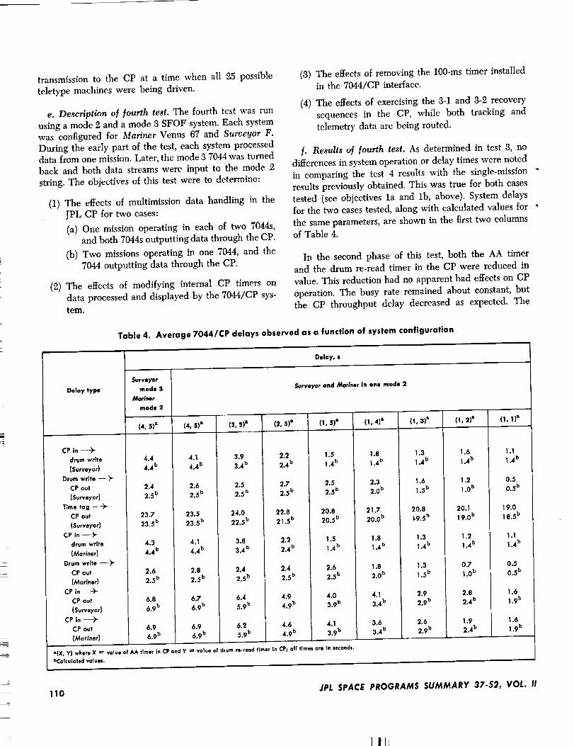
transmission to the CP at a time when all 25 possible

teletype machines were being driven,

e. Description of fourth test. The fourth test was run

using a mode 2 and a mode 8 SFOF system. Each system

was configured for Mariner Venus 67 and Surveyor F.

During the early part of the test, each system processeddata from one mission. Later, the mode 3 7044 was turned

back and both data streams were input to the mode 2

string. The objectives of this test were to determine:

(I) The effects of multimission data handling in the

JPL CP for two cases:

(a) One mission operating in each of two 7044s,

and both 7044s outputting data through the CP.

(b) Two missions operating in one 7044, and the

7044 outputting data through the CP.

(2) The effects of modifying internal CP timers on

data processed and displayed by the 7044/CP sys-tem.

(8) The effects of removing the 100-ms timer installed

in the 7044/CP interface.

(4) The effects of exercising the 8-1 and 8-2 recovery

sequences in the CP, while both tracking and

telemetry data are being routed.

[. Results o[ fourth test. As determined in test 8, no

differences in system operation or delay times were noted

in comparing the test 4 results with the single-mission

results previously obtained. This was true for both cases

tested (see objectives la and lb, above). System delays

for the two cases tested, along with calculated values for

the same parameters, are shown in the first two columnsof Table 4.

In the second phase of this test, both the AA timer

and the drum re-read timer in the CP were reduced in

value. This reduction had no apparent bad effects on CP

operation. The busy rate remained about constant, but

the CP throughput delay decreased as expected. The

Table 4. Average 7044/CP delays observed as a function of system configuration

Delay, I

Delay type Surveyor and Mariner In one mode 2

(3, 5)e (2, 5)a (1, 5)a (I, 4)s (1, 3) a (!, 2) a (!, 1)a

CP in

drum write

{SurVeyor}

Drum write

CP out

(Surveyor)

Time tag

CP out

(Surveyor)

CP In

drum write

(Mariner)

Drum write

CP out

iMariner)

CP In -_-

CP out

(Surveyor)

CP in

CP out

(Mariner)

Surveyor

mode 3

Mariner

mode 2

(4, 5) a (4, 5)B"

4.4 4.1

4.4 b 4.4 b

2.4 2.6

2.5 b 2.5 b

23.7 23.5

23.5 b 23.5 b

4.3 4.1

4.4 b 4.4 b

2.6 2.8

2.5 b 2.5 b

6.8 6.7

6.9 b 6.9 b

6.9 6.9

6.9 b 6.9 b

l(X, Y) where X ----"value of AA tlmer in CPand Y =s value of drumbCalculateclvalues.

3.9

3.4 b

2.5

2.5 b

24.0

22.5 b

3.8

3.4 b

2.4

2.5 b

6.4

5.9 b

6.2

5.9 b

2.2

2.4 b

2.7

2.5 b

22.8

21.5 b

2.2

2.4 b

2.4

2.5 b

4.9

4.9 b

4.6

4.9 b

1.5

1.4 b

2.5

2.5 b

20.8

20.5 b

1.5

1.4 b

2.6

2.5 b

4.0

3.9 b

4.1

3.9 b

1.8

1.4 b

2.3

2,0 b

21.7

20.0 b

1.8

1.4 b

1.8

2.0 b

4.1

3.4 b

3.6

3.4 b

re.read timer In CP; all times ore In seconds,

1.3

1.4 b

1.6

1.5 b

20.8

'_9.5 b

1.3

1.4 b

1.3

1.5 b

2.9

2.9 b

2.6

2.9 b

1.6

1.4b

1.2

1.0 b

20.1

19.0 u

1.2

1.4 b

0.7

1.0 b

2.8

2.4 b

1.92.4 b

1.1

1.4 b

0.5

0.5 b

19.0

18.5 b

1.1

1.4 b

0.5

0.5 b

1.6

1.9 b

1.6

1.9 b


last seven columns in Table 4 show these delays, along

with the calculated values for the same parameters.

In an abbreviated test with the 100 ms delay removed

from the 7044/CP interface, the system performed as

expected, and message segment frequency, during maxi-

mum interface activity periods, was increased by a factor

of four. The test showed that the original reason for the

delay's insertion no longer exists.

In SPS 87-51, Vol. II, pp. 96-98, it was stated that the

79-s 7044 delay of telemetry data was a worst-case con-

dition during predict transmission. This statement was

not true. In test 4, a larger block of predicts was trans-

mitted to the CP. The 7044 delay at its output interface

increased to a maximum of 14.5 s. This figure would beeven higher if the Mariner data rate had been 81_ insteadof :33_ bits/s.

Several 8-2 and 3-1 recoveries on the CP were at-

tempted on the CP. Telemetry and tracking data were

not stopped during these attempts. The following ob-servations were made:

(1) The STOP ALL message from the 7044 was not

necessary during the recoveries.

(2) During all 3-2 recovery attempts, the CP and 7044

ran into accounting problems with the tracking

data. It appeared that the CP was recycling mes-

sage numbers for these data and causing the data

to go to intercept. The program is not supposed tooperate in this manner.

(8) As before, only one of three 8-1 recoveries was

even partially successful. A reload was required in

two cases. In the partially successful recovery, the

written procedure was followed; however, the op-

erator had to perform a number of extra manual

operations to get the system completely back tooperational status.

It was observed that a given 7044 can output data to

up to 50 data sinks through the CP; however, the CP is

incapable of routing these data to more than 25 machines

due to the length of a queuing list in the machine.

g. CP statistics from fourth test. The maximum of

25 simultaneous drum input/output requests was made.

Had all the conditions been exactly wrong, this number

could have been as high as 56. The maximum of 62 timerlist entries was used. This number could have been as

high as 65 for the configuration used. The maximum of

56 pack areas was used, and the maximum of 18 vali-

dation queue entries was made.

During high-activity periods, the busy rate averaged

80%. The maximum rate of 90% occurred duringpredict transmission.

B. Deep Space Instrumentation Facility

1. Venus OSSActivities, E.B.Jackson, M. A. Gregg, and A. I. Price

a. Experimentation. The 80-ft-diam antenna continued

to be used for transmission of time synchronization sig-nals at 8.45 CHz and for radiometric observations of the

planet Venus at 28 GHz. Successful planetary radar oper-

ations were resumed with good total spectrum returns

being received from the planets Venus and Mercury in

both monostatic and bistatic modes of operation. Figure 2

illustrates the typical monostatic return, and Fig. 8 illus-

trates the typical bistatie return. The improvement in

signal-to-noise ratio generated by the additional 8-dB

gain of the 210-ft-diam antenna for receiving is clearlyseen.

Taking advantage of an opportunity which only occurs

every 19 yr, the 85-ft-diam antenna and the 450-kW trans-

mitter were used to transmit radar signals to the asteroid

Icarus. Closest approach of 6,858,270 km was predicted

to occur at approximately 2058Z on June 14, 1968. At that

time, assuming an asteroid diameter of 1 km and a radar

reflectivity at 2888 MHz of 100%, the received signal

strength, using the 210-ft-diam antenna at the Mars DSS,

would have been approximately -181 dBm. Completeresults from this mission are not available at this time.

Preliminary data indicate that the actual received signalstrength was - 187 dBm.

b. Subsystem performance. The Venus DSS S-band

2388-MHz receiver provides one phase-locked channel

and two open-loop channels. In addition, the special

455-kHz loop in the receiver can provide some phase-

locked information when operating in the open-loop

mode. The receiver still retains the capability of accept-

ing 455-kHz signals, via the microwave link, from either

of the two R&D receivers at the Mars DSS when operat-

ing in the bistatic mode.

The 8448-MHz X-band receiver continues to serve as

an X-band transmitter output and modulation monitor in

the time synchronization experiment. The operation of

the transmitter phase modulator was checked during this

reporting period. The carrier power suppression was


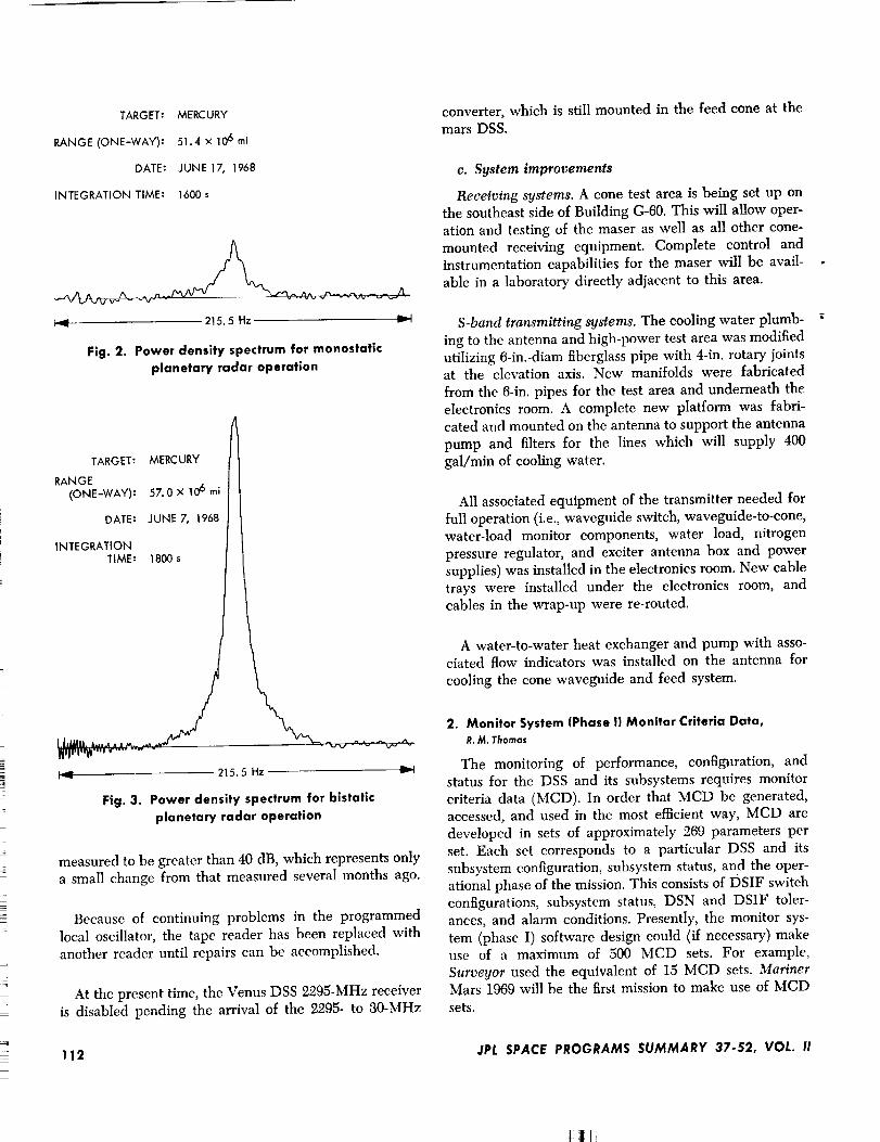
TARGET: MERCURY

RANGE (ONE-WAY): 51.4 × 106 ml

DATE: JUNE 17, 1968

INTEGRATION TIME: 1600 s

,_'_" 215.5 Hz ,._',

Fig. 2. Power density spectrum for monostatlc

planetary radar operation

TARGET:

RANGE

(O N E-WAY):

DATE:

INTEGRATION

TIME:

i_.Jl

MERC URY

57.0 × 106 mi

JUNE 7, 1968

1800 s

215.5 Hz ""_'

Fig. 3. Power density spectrum for bistatic

planetary radar operation

measured to be greater than 40 dB, which represents only

a small change from that measured several months ago.

Because of continuing problems in the programmed

local oscillator, the tape reader has been replaced with

another reader until repairs can be accomplished.

At the present time, the Venus DSS 2295-MHz receiver

is disabled pending the arrival of the 2295- to 30-MHz

converter, which is still mounted in the feed cone at themars DSS.

c. System improvements

Receiving systems. A cone test area is being set up on

the southeast side of Building G-60. This will allow oper-

ation and testing of the maser as well as all other cone-

mounted receiving equipment. Complete control and

instrumentation eapabilities for the maser will be avail-

able in a laboratory directly adjacent to this area.

S-band transmitting systems. The cooling water plumb-

ing to the antenna and high-power test area was modified

utilizing 6-in.-diam fiberglass pipe with 4-in. rotary jointsat the elevation axis. New manifolds were fabricated

from the 6-in. pipes for the test area and underneath the

electronics room. A complete new platform was fabri-

cated and mounted on the antenna to support the antenna

pump and filters for the lines which will supply 400

gal/min of cooling water.

All associated equipment of the transmitter needed for

full operation (i.e., waveguide switch, waveguide-to-eone,

water-load monitor components, water load, nitrogen

pressure regulator, and exciter antenna box and power

supplies) was installed in the electronics room. New cable

trays were installed under the electronics room, and

cables in the wrap-up were re-routed.

A water-to-water heat exchanger and pump with asso-ciated flow indicators was installed on the antenna for

cooling the cone waveguide and feed system.

2. Monitor System (Phase !) Monitor Criteria Data,R. M. Thomas

The monitoring of performance, configllration, and

status for the DSS and its subsystems requires monitor

criteria data (MCD). In order that MCD be generated,

accessed, and used in the most efficient way, MCD are

developed in sets of approximately 269 parameters per

set. Each set corresponds to a particular DSS and its

subsystem configuration, subsystem status, and the oper-

ational phase of the mission. This consists of DSIF switch

configurations, subsystem status, DSN and DSIF toler-

ances, and alarm conditions. Presently, the monitor sys-

tem (phase I) software design could (if necessary) make

use of a maximum of 500 MCD sets. For example,

Surveyor used the equivalent of 15 MCD sets. MarinerMars 1969 will be the first mission to make use of MCD

sets.

112 JPL SPACE PROGRAMS SUMMARY 37-52, VOL. !1

III

These data are generated in the SFOF and put on a

magnetic tape, which is shipped to the DSS. Upon ar-

rival at the DSS, a tape-to-tape program will take the MCD

parameters from the magnetic tape and put them on a dual

cartridge magnetic tape recorder (Mag Pak). The desired

set is then selected and called into working memory by

the DSS computer operator. Accessing any parameter(s) of

a given set is accomplished by utilizing the format dis-

cussed later in this article. Each DSS will only have onenonstandard MCD set. A nonstandard set is defined as

the set that was called into auxiliary core, modified, and

is currently being used in working core (memory). A

capability exists for changing 82 critical MCD param-eters in real time.

Either the SFOF or DSS operator can change these

82 parameters as follows, but in either case the DSS

operator must put the modified set in working core if it

is going to be used. The DSS operator will be able to:

(1) take an MCD set from the magnetic pack and put it

in working core, (2) take the MCD set in auxiliary core

and put it in working core, and (8) change any one or all

of the 32 critical MCD parameters in working core. The

SFOF will be able to do the following in real time:

(1) call an MCD set from the Mag Pak and place it in

auxiliary core and modify the MCD set, (2) modify the

existing MCD set in auxiliary core, and (3) define a new

MCD set, transmit it to the DSS, and place it in auxiliary

core. The DSS and SFOF capabilities explained above

can be represented diagramatically (Figs. 4 and 5).

When generating the MCD to be put on magnetic tape

(from the disk file) by a 7094 computer program, only

one MCD parameter is placed on each card. Hence, the

sets of desired MCD parameters are punched on cards,

read by a card reader, and placed on magnetic tape by

the 7094 program. These tapes will have a two-fold

purpose: (1) the tapes will serve as a master record

MMCD (master monitor criteria data) file, and (2) a

direct copy will be shipped to the DSS for use as pre-viously discussed.

SFOF real-time MCD updating can be accomplished

from either disk (mode 2) or magnetic tape (mode 4).

In mode 2, the 7044 requests the MCD from the 7094,which in return gets the MCD from the disk file and

gives it back to the 7044 and then to the TTY for trans-

mission to the station. Using mode 4, the 7094 puts the

MCD on tape, and the tape is physically transported to

the 7044 and peripheral equipment for accessing and

transmitting to the station by TTY via the 7044. Generally,

mode 4 wilI be used. The user (in mode 2 or 4) will ask

that a message be prepared and transmitted via the 7044

GET MCD FROM_

PUT MCD IN

WORKING

CORE

WORKING

CORE

AUXILIARY

CORE

2HANGE ANY OR ALL

OF 32 CRITICAL MCD

PARAMETERS IN

WORKING CORE

PLACE MCD FROM

AUXILIARY INTO

WORKING CORE

Fig. 4. DSS MCD capabilities

PUT MCD SET PUT NEW SFOF - J J PUT ANY MODIFIED

IN AUXILIARY' DEFINED MCD SET J J MCD SET IN

CORE IN AUXILIARY CORI I I AUXILIARY CORE

WORKING II

CORE [lAUXILIARY CORE V

MODIFYANYMCDSEtINAUXlUAR¥CORE

Fig. 5. SFOF MCD capabilities

by TTY to the digital instrumentation subsystem (DIS).

The MCD address structure aids in accessing and modi-

fying of any parameter(s) of any set. This address structure

consists of set, subset, parameter address, computer word,

bit position, parameter value, condition, and format.To change any MCD parameter, the SFOF operator would

input the set, subset, parameter address, and parametervalue.

A typical set" of MCD would consist of:

(1) Configuration (DSIF switch positions) and sub-

system status parameters for microwave, trans-

mitter, receivers 1 and 2, doppler (1-, 2-, and 8-way),

angle (hour angle and declination), ranging, sub-

carrier demodulator assembly (SDA 1, 2, 3, and 4),

telemetry and command processor (TCP 1 and 2),

and the automatic data switching systems a and/3.


(2) Tolerances and nominal (expected) values are alsocontained in each set for the transmitter receiver,

automatic gain control/static phase error, doppler

(1-, 2-, and 8-way), angle (hour angle and declina-

tion), ranging, TCP, SDA, DIS, RF, and telemetry

predicts.

3. DSIF/Ground Communications Interface Assembly,E. Garc_a

a. Introduction. Previous articles (SPS 8%50, Vol. II,

pp. 168--172, and SPS 87-51, Vol. II, pp. 100-104) have

presented the DSIF/ground communications interface

assembly (DGI) functional requirements, theory of oper-

ation, implementation plans, and a detailed descriptionof the DGI buffer cabinet assembly. This article presents

a description of the DGI buffer assembly new module

development.

Four new module types are being developed, in orderto meet functional and interface requirements of the DGI

and external interfacing subsystems. The new modules

are being constructed with enough flexibility and to thesame mechanical and electrical specifications of the Hi-Rel

module line such that they may be used in future projects.

b. Level converter. The level converter (LC-38) module

has been developed to meet the interface requirement to

drive other assemblies with bipolar signals. The LC-88module contains six identical interface circuits. Each

unit is designed to condition a unipolar logic input level

and produce a bipolar logic output level. The units are

designed by Dynamics Instrumentation Co., and usehigh reliability components that have been burned-infor 168 h.

The level converter electrical characteristics per circuit

are as follows:

Power input

Signal input

Signal output

Output impedance

Rise and fail time

Input/output logic

+12Vdc +_10% at 15mA

- 12 Vdc ___10% at 15mA

0 to + 25 Vdc maximum at 0.5 mA

or less; threshold of +4.0 ___0.5 V

+ 6 +__0.5 to - 6. ___0.5Vdc; short-

circuit proof

100 t2 or less

1 _s or less

+ 4.5 V or greater input produces

+6-V output; +3.5 V or less

produces - 6-V output

c. Signal generator. The signal generator (SG-270)

module has been developed to meet the Mariner Mars

1969 270-Hz telemetry bit rate, for use as a DGI-simulated

output data clock. The SG-270 module contains one

sealed can-type module manufactured by CTS Knight

Corp. The basic crystal oscillator is cut for a frequency

of 2.7 MHz. By use of integrated circuits, four output

frequencies are brought out. All components are burned-

in for 168 h at +125°C and are chosen from the ]PLHi-Rel Preferred Parts List.

The signal generator electrical characteristics are asfollows:

Power input

Signal output

Frequency stability

Output wave shape

+ 12 Vdc ± 10% at 2.5 mA

--12 Vdc __+10% at 2.5 mA

270,000 Hz at 0 to + 5 ±0.5 Vdc

squarewave

27,000 Hz at 0to +5 ±0.5 Vdc

squarewave2700 Hz at 0 to +5 ±0.5 Vde

squarewave270 Hz at 0 to + 12 Vdc ± 10%

squarewave

±50 parts per million; after in-

itial stabilization period, fre-

quency is 8 parts in 10_ per

day for one yr

50 ±2% duty cycle with a bitwidth distortion of ___1% or less

d. Shift register and word detector. The shift register(SR-33) and word detector (WD-33) modules have been

developed to meet the DGI requirement for a hardware

24-bit word syne detection capability. The DGI sync

word detection function is mechanized using three SR-88s,

eight bit shift register modules, and one word detector

module. The function performed is that of comparing a

serial bit stream every bit time (sample rate of 1 MHz)

to a predetermined bit pattern configuration of 24 bits. A

correlation output signal is provided out of the WD-88

module, whenever the input serial bit stream correlates

to within 0, 1, 2, or 3 preprogrammed allowable random

errors of the 24-bit pattern configuration.

These two basic-type modules are being manufactured

by Space General Corp., and make use of discrete and

integrated circuit components. All components erfiployedare chosen from the JPL Preferred Parts List and undergo

a 168-h burn at +125°C in screening tests.


Shift register. The shift register module contains an

8-bit shift register, eight clocked nand gates, and eight

wired or hand gates. The module is designed to perform

five basic functions by means of jumper wires: (1) serial

input/parallel output, (2) parallel input/serial output,

(8) serial input/clocked parallel output, (4) clocked par-

allel input/serial output, and (5) preset 8-bit word gen-erator. Its electrical characteristics are:

Input power

Parallel input

Serial input

Serial output

Ored nand output

Clock input

Parallel output

+12 Vdc __+10% at 15 mA

0 to + 12 __+3Vdc input (type I)0to +5 ±1 Vdc input (type II)

0 to + 5 __+1 Vde

0 to + 5 ± 1 Vdc

0 to +5 __+1Vdc

0 to + 5 ± 1 Vdc; squarewave upto 3 MHz

Clocked 0 to + 5 ± 1 Vdc

Direct 0 to + 5 ± I Vdc

Word detector. This module was designed as a special-

purpose module containing all logic elements required

to complement any number of SR-33 modules inter-

connected as a word pattern correlator. Thus, it contains

the necessary input data clock-sample clock synchro-

nization circuit, SR-88 shift clock amplifiers, start-stop

2-bit shift register, 3-bit decimal counter, and 8-bit deci-

mal comparator. Its uses as part of the standard Hi-Rel

line are limited; however, this limitation was acceptedin order to make the SR-33 module more versatile. The

word detector electrical characteristics are:

Power input

Data clock

input (fd)

Sample clock

input (fs)

Word detection

at = (f8 - fd)

2-bit shift register

input

8-bit decimal com-

parator input

Clock amplifier

output

+12Vdc -+-10% at 80mA

0 to + 12 ±3 Vdc squarewave;

50 ±2% duty cycle

0 to + 12 __+5Vdc squarewave;

50 ___2% duty cycle

±f minimum must equal in Hz the

number of bits in word input

plus 2 cycles for start-stop

0 to +5 ±0.5 Vdc

0 to +5 +__0.5 Vdc for each line;

only one line at +5 Vdc at a

time for correct comparison

0 to +5 -+-0.5 Vdc at 80mA

4. DSIF Station Control and Data Equipment,E. Bann, A. T. Burke, ]. K. Woo, and P. C. Harrison

a. Antenna pointing subsystem phase I. The antenna

pointing subsystem (APS) has been implemented in the

DSIF stations to provide the capability of pointing

the station antennas under computer control. Descrip-

tions of the interim APS and the APS phase I (APS-I)have been given in previous issues of SPS, Vol. II.

Acceptance testing of APS interface (API) racks is

essentially complete, and API units have been accepted

for all station commitments at the Echo, Woomera, Tid-

binbilla, Johannesburg, Robledo, and Cebreros DSSs.

Installation of APS-I is being accomplished in three

steps: (1) first the SDS 910 computer is separated from

its digital instrumentation subsystem (DIS) phase I con-

figuration and retrofitted to a standard SDS 910 com-

puter, (2) the API rack is then connected to the SDS 910

computer and an APS-I diagnostic is performed to ensure

correct operation at the unit level, and (3) finally, the

station system cables are installed and testing is com-pleted with APS-I in its operational configuration utiliz-

ing its operational program. Steps 1 and 2 have been

completed at the Echo and Johannesburg DSSs and will

be completed at the Woomera and Cebreros DSSs by the

end of July 1968. The installation at the Tidbinbilla and

Robledo DSSs does not include Step 1, since the DISs

are not being updated at this time.

b. Telemetry and command processor phase 1I. The

Telemetry and Command Processor Phase II (TCP-II)

provides the DSIF with a mission-independent telemetry

and command processing capability for real-time oper-

ation. The TCP-II is in the process of expansion (TCP-II-C) to increase the telemetry processing capability to

support the DSIF multiple-mission telemetry system.

The installation of the TCP-II-C equipment is pro-ceeding on schedule at the DSSs. Installation and check-

out has been completed at the Echo, Cape Kennedy, and

Johannesburg DSSs and is currently in process at theCebreros DSS. The TCP-II-C equipment has been

shipped to the Woomera DSS.

The necessary equipment to implement the change-

over from a 60-wpm teletype operation to a 100-wpm

operation has been supplied to all DSSs.

c. Frequency and timing subsystem phase II. The fre-

quency and timing subsystem phase II (FTS-II) was


subjected to a design review and was accepted as pre-

sented. Evaluation of the FTS-II prototype is continuing

at the contractor's facility with the resultant logic pulse

jitter maximum of 10 ns with respect to the selected

frequency source.

(4) Control room rebuilding: re-installation of new

and old cables, modification and relocation of

equipment, and addition of cable trays.

(5) Station integration testing: verification that the

station is configured and functions as specified.

Assembly of the production equipment is underwayand the preliminary testing of some of the subassemblies

has been accomplished.

5. Echo DSS Reconfiguration, F.M.$chiffman

a. Introduction. The Echo DSS is the first DSIF sta-

tion to start the engineering modification and upgrade

(reconfiguration) in support of future spacecraft missions

such as Mariner Mars 1969. The Echo DSS reconfigura-

tion was started in early February 1968 and is expectedto be completed by mid-July 1968. A series of station

integration tests are scheduled to validate system, sub-

system, and equipment reconfiguration.

b. Obiectives. The objectives of the Echo DSS recon-figuration are:

(1)

(2)

To provide required support capability for the

Mariner Mars 1969 mission (primary objective).

To implement a number of subsystem modifica-tions, other than those required for the MarinerMars 1969 mission.

(3) To perform the equipment maintenance hereto-

fore precluded by station mission support assign-ments.

(4)

(5)

To facilitate and complete subsystem transfer

agreements from engineering to operations.

To configure each of the effected stations consistent

with the Goldstone-duplicate-standard concept.

c. Modification phases. The Echo DSS reconfiguration

included five distinct modification phases, which were:

(1) Antenna teardown: removal of antenna mounted

equipment, cables, and water lines.

(2) Control room teardown: removal and inspection of

cables and equipment.

(3) Antenna rebuilding: re-installation of cables and

trays, equipment, hydraulic and water lines, and

addition of new declination room and equipment.

116

d. Subsystem modlfications.Eight subsystems required

modification during the Echo DSS reconfiguration asfollows:

Subsystem Modification

Antenna mechanical

Telemetry command

processor

Digitalinstrumentation

Receiver III-C

Demultiplexer

Simulator I

Upgrade hydraulic drive

Upgrade hour angle and decli-nation drive skids

Thicken structure of supportmembers

Rebolt

Limit polar wheel travel (-+-89

to ±105 deg)

Add new cable wrapups

Resurface and align dish

Adjust limit switch and optical

tracking aid

Add declination room

Remove existing 8k core mem-

ory and install 16k core

Add analog equipment rack andcables

Remove SDS 910 computer

Modify rate selection and pe-riod register

Increase core from 8 to 16k

Add magnetic pack

Add communications buffer

Install subcarrier demodulator

Install analog-to-digital con-verters

Install digital phase shifters

Install new demultiplexer

Install new simulator I

e. Control room layout. Figure 6 illustrates the recon-

figured Echo DSS control room layout.

JPL SPACE PROGRAMS SUMMARY 37-52, VOL. I!

tll,

_ -

_-z _ _-_

,-_ _, _ _ _,- _zz_ b_= _

0

.q

_q_.EC.EI_iNG PAGE BLANK NOT FiLJ,,'I_D.

C. DSN Systems and Projects

1. MMTS: Installation and Testing, w. c. rrer

a. Introduction. Installation of the multiple-mission

telemetry system (MMTS) includes verifying proper

operation of: (1) the subcarrier demodulator assemblies

(SDAs), two of which are required per station; (2) the

MMTS test rack; and (3) the telemetry command pro-

cessor (TCP) in the phase II-C configuration, including

the digital phase shifters. In addition, all MMTS func-tional interfaces are checked between the SDAs and the

TCP, the SDAs and the digital instrumentation subsystem

. (DIS), and between the TCP and the DIS. Functionalinterfaces are verified using MMTS project-supplied soft-

ware operating in the DIS and TCP computers.

Testing of the MMTS equipment is accomplished in

three phases: (1) checkout of the computer and digital

equipment with MMTS demonstration software; (2) test-

ing of the SDA, combined with the computer and digital

equipment, with test signals input through the SDA up-converter; and (3) checkout of the SDA combined with

the computer and digital equipment, with signals from the

receiver applied to the 10-MHz telemetry input of the

SDA.

b. Computer and digital equipment tests. In order to

evaluate the computer and digital equipment perform-

ance, the MMTS demonstration software has been

modified to operate in the TCP phase II-C equipment

configuration. The software performs the bit synchro-

nization and detection functions. The program outputs

bit error rate and an estimate of signal-to-noise ratio.

The demonstration software has been implemented as an

MMTS test program in the DSN. A test signal input of

an integrated PN data stream, with noise added, was

provided to the analog-to-digital converter input of the

TCP. The input signal-to-noise ratio was calibrated,

using the signal-to-noise ratio estimator (SNORE) pro-

gram in the TCP. The SNORE program has also been

modified to be compatible with the TCP phase II-C. The

SNORE program runs with hard-wired bit sync and

detection and provides an excellent reference for the

input signal-to-noise ratio of test signals supplied to theTCP.

The MMTS demonstration program performance was

then compared to the SNORE program. The output of

the demonstration program of bit error rate and signal-to-

noise ratio indicated performance agreement with theSNORE reference within 0.1 dB at all stations; thus,

the bit syne and detection functions performance were

verified as operating properly in the TCP phase II-C

configuration. The tests were run at STJNo of 5.2 dB at270 bits/s.

c. SDA/TCP phase II-C up.converter tests. Tests were

conducted using the baseband input (up-converter) of

the SDA to verify performance of the SDA and its oper;

ation in conjunction with the demonstration software in

the TCP phase II-C. The up-converter input consisted of

a PN data stream modulating a subcarrier, with noise

added. The performance of the system was measured by

the signal-to-noise ratio estimate of the MMTS demon-

stration software located in the TCP. The following data

were obtained for the JPL compatibility test area and are

typical for all stations:

Test

Bit Subcarrier

rate, frequency,bits/s kHz

1 270

2 270

8 66.66

4 33.33

5 8.33

84

84

84

24

24

Up-converter

inputSTJNo, dB

5.2

-1.0

5.2

5.2

5.2

Measured

STJNo bydemonstra-

tion soft-

ware, dB

4.62

- 1.48

4.61

4.48

4.32

The degradations encountered in this test mode are

primarily due to the uncertainty of the calibration of the

signal-to-noise mixer and to dynamic range limitations

of the up-converter. The test data taken at the stationsare within the + and - 1-dB tolerance allowed in set-

ting up the signal-to-noise ratio.

d. System tests. System testing involved use of the

receiver 10-MHz telemetry output as a signal source for

the MMTS equipment. The telemetry modulation inputof the test transmitter was used as input for a subcarrier

modulated with data test signal input. Signal-to-noise

ratio in the carrier tracking loop was measured for a

calibration of input STJNo.

The MMTS demonstration program was used to mea-

sure system performance. Results of these tests indicate

that MMTS performance is within specifications after

the known degradations of the receiver and the MMTS

equipment have been introduced into the resultant data.

Additional reporting on the system tests will be presentedin a future SPS article.

JPL SPACE PROGRAMS SUMMARY 37-52, VOL. il 119

e. DSS implementation. Installation and checkout of

the new MMTS have been completed on schedule at the

compatibility test area, as well as at the Echo, Cape

Kennedy, Johannesburg, Cebreros, and Woomera DSSs.Installation and checkout of the new MMTS at the Mars

DSS is scheduled to begin in early September. The

Tidbinbilla and Robledo DSSs will be provided with

MMTS in February 1969.

2. MMTS: SDA/Receiver-Exciter Interface, j. H. Wifcher

a. Introduction. The installation of the subcarrier

demodulator assemblies (SDAs) as part of the receiver-

exciter subsystem requires that portions of the receiver-exciter be modified to interface with the SDAs.

b. Receiver-exciter modifications. Each SDA requires

the following signals from the receiver-exciter subsystem:

Function Level

10-MHz reference

10-MHz IF (receiver 1)

10-MHz IF (receiver 2)

5-MHz reference

Switching

Lamp

10 dBm

- 66 dBm

- 66 dBm

10 dBm

28 Vdc

24 Vde

Since the number of SDAs which will be interfaced

with the receiver--exciter varies from one to four, the

SDA/receiver-exciter modification kits were designed tohandle four SDAs at all sites.

Four unused 10-MHz reference signals were availableat cabinet 8 of the receiver-exciter for use with the

J4

J5v

J..._2___1

120

A401

50-MHz

IF AND

SECOND

MIXER

A402

10-MHz IF

DISTRIBUTIONAMPLIFIER

A403

10-MHz FILTER

AMPLIFIER

PRESENT

J4

J2 J SDANARROW BAND TELEMETRY

J3 SDA

RANGING

J4 SDA

WIDE BAND TELEMETRY J9

MODIFICATION

A401

50-MHz

IFAND

SECOND

MIXER

J1 t A402

I 0-MHz IF

SIGNAL

DISTRIBUTION

AMPLIFIER

SDA

J--"_'_l_ NARROW BAND TELEMETRY

RANGING

WIDE BAND TELEMETRY

IIIII

Fig. 7. SDA/recelver-exclter functional interface (cabinets 5 and 8)

A403

J1

10-MHz FILTER

AMPLIFIER

JPL SPACE PROGRAMS SUMMARY 37-52, VOL. I!

I|!

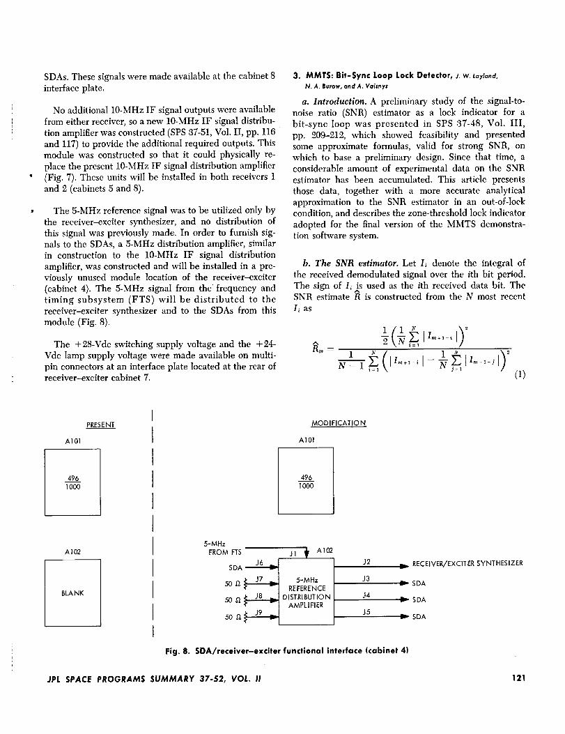
SDAs. These signals were made available at the cabinet 8

interface plate.

No additional 10-MHz IF signal outputs were available

from either receiver, so a new 10-MHz IF signal distribu-

tion amplifier was constructed (SPS 37-51, Vol. II, pp. 116

and 117) to provide the additional required outputs. Thismodule was constructed so that it could physically re-

place the present 10-MHz IF signal distribution amplifier

(Fig. 7). These units will be installed in both receivers 1

and 2 (cabinets 5 and 8).

The 5-MI-Iz reference signal was to be utilized only by

the receiver--exciter synthesizer, and no distribution of

this signal was previously made. In order to furnish sig-

nals to the SDAs, a 5-MHz distribution amplifier, similar

in construction to the 10-MHz IF signal distribution

amplifier, was constructed and will be installed in a pre-

viously unused module location of the receiver-exciter

(cabinet 4). The 5-MHz signal from the frequency and

timing subsystem (FTS) will be distributed to the

receiver-exciter synthesizer and to the SDAs from this

module (Fig. 8).

The +28-Vdc switching supply voltage and the +24-

Vdc lamp supply voltage were made available on multi-

pin connectors at an interface plate located at the rear ofreceiver-exciter cabinet 7.

3. MMTS: Bit-Sync Loop Lock Detector, j. w. tayland,N. A. Burow, and A. Vaisnys

a. Introduction. A preliminary study of the signal-to-

noise ratio (SNR) estimator as a lock indicator for a

bit-sync loop was presented in SPS 37-48, Vol. III,

pp. 209-212, which showed feasibility and presented

some approximate formulas, valid for strong SNR, on

which to base a preliminary design. Since that time, a

considerable amount of experimental data on the SNR

estimator has been accumulated. This article presents

those data, together with a more accurate analytical

approximation to the SNR estimator in an out-of-lockcondition, and describes the zone-threshold lock indicator

adopted for the final version of the MMTS demonstra-

tion software system.

b. The SNR estimator. Let If denote the integral of

the received demodulated signal over the ith bit period.

The sign of Ii is used as the ith received data bit. TheSNR estimate _ is constructed from the N most recent

I_ as

RIt_

1 1 tN-11":1 j =1

(1)

PRESENT

AI01

496

1000

A102

BLA NK

MODIFICATION

AI01

496

1000

5-MHz

FROM FTS

SDA

50D,_

50 9, ¢_..-LI_

5o 9, ¢_--I_

J1 _ A102

5-MHz

REFERENCE

DISTRIBUTION

AMPLIFIER

J2

J3

J4

J5

RECEIVER/EXCITER SYNTHESIZERv

SDA

SDA

SDA

Fig. 8. SDA/receiver-exciter functional interface (cabinet 41


where J x I denotes the absolute value of x. The averagingover N bit periods could equivalently be a digital low-

pass filter with "time constant" equal to N bit periodswith no significant change in the results. Let R be the

true SNR and assume the local bit-timing reference is

perfectly synchronized with the received signal. Then, asN grows large, the estimator R converges in probability

to the function R*(R), plotted in Fig. 9.

{R'_[1 - 2 erfc (2R) 1/_] + 7r-_ e-R} z

R*(R) - 1 + 2 (R - {Rv_[1 - 2 erfc i2R) 1/2] + _--'_ e-R) "-')

(2)

A similar result can be obtained if a bit timing offset

exists. Let that offset be 8, in fractions of a bit duration,

and assume that data sign transitions occur with proba-

bility p at each of the possible transition points. If notransition falls within the time interval of the bit integral

I_, its mean and variance are identical to what they

would have been with no timing offset. If a transition

occurs there, however, the signal amplitude is reduced

by the factor (1- 2j0 ]), while the noise variance isunaffected. Let

8

v 4

00 ! 2 3 4 5 6 7

R = ST/N 0

Fig. 9. Asymptotic value of the estimator R vs R

A(R,,O) -- p(R"_(1 -- 2J61) {1 - 2erfc [(2R) '_" (1 - 2[ _[)1} + _--_'2exp [- R(1 - 2[01)_]) )

+ (1 -- P) {R''_ [1 - 2 erfc (2R) v_] + _'-"_ e -_ }

B(R,e) = a[p(1 - 2 l e[) 2 + (1 - p)]

(3)

Then, if a static offset of 0 is maintained, it can be easily

shown that the SNR estimate R will converge in proba-

bility to

a2(a,o)a*(R,0) = i + 2[B(R,O)- A_(a,0)] (4)

Further, let

J_aA,(a) -- doA(a,o)

B,(R) = d0 B(R,0)

(_)

Then, ff the bit timing loop is slowly slipping cycles

throughout the measurement period, and enough cycles

are slipped throughout this period that the distribution

of static timing offset is essentially uniform, the SNR

estimate R will converge in probability to

A_ (R)R: (R) -- 1 + 2[B,(a) - A_ (a)] (6)

For large R, Eqs. (4) and (6) reduce to Eqs. (18) and (14)

of SPS 87-48, Vol. III, pp. 211-212, respectively. R*(R,a)

is plotted in Fig. 10 as a function of a for various values

of R. Certain special points are marked on _ach of the

lines denoting an input SNR: "+" denotes the value of

R_(R) associated with this input SNR, calculated bynumerical integration; "0" denotes the median experi-

mental value for _,(R).

c. Experimentat distribution of R. Values of R(R) and

R,(R) were obtained experimentally for input SNRs of

2.5, 5.2, 7.5, and 10.0 dB. The samples making up eachwere filtered in a bandwidth equivalent to 0.8% of the

bit rate for input values of St/No >__7.5 dB and 0.1% of

the bit rate for input values of St/No > 7.5 dB. Distribu-tions for each test contain a minimum of 10,000 inde-

pendent samples. For convenience, a bit rate of 250 bits/s


I|1

I0

103

O EXPERIMENTAL CYCLE SLIPPING

-k COMPUTED CYCLE SLIPPING

I0

1.8

1.0

0

0.25

8

Fig. 10. R*(R,_)vs_forR = 1 to 10 '_

0.Su


10

6

4

2

0

--T TBITSYNC LOOP

I I

O TRACKING

[] CYCLESLIPPING-

O

[]

0 2

0 _ PROPOSED

T6 8 I0

INPUTST/N0, dB

THRESHOLDS

oO

Fig. 11. Mean values of the experimental _ distributions

for loop in lock and cycle slipping

4. MMTS: 10-MHz Quadrature Generator and Phase

Switch, R.B.Crow

A 10-MHz quadrature generator and phase switch

has been developed for the subcarrier demodulator

assembly (SPS 37-46, Vol. III, pp. 221-230) to be used in

the multiple-mission telemetry system.

The block diagram of the quadrature generator and

phase switch (Fig. 13) illustrates that it is a small sub-

system packaged in a single module. The purpose of the

unit is to act as a signal phase switch to demodulate

(1) the subcarrier in the data channel (0-deg channel) so

that the output of the unit is 10-MHz X data, (2) the

subcarrier in the quadrature channel (270-deg channel)

so that the output of the unit is 10-MHz X data, and

(3) the product of subcarrier X data in the error channel

(90-deg channel) so that the output is a 10-MHz signal.

was arbitrarily selected. For the cycle slipping case, the

offset was 3.6% of the bit rate. The means of R(R) and

Rs(R) are plotted in Fig. 11, and the distributions are

plotted in Fig. 12.

d. Zoned lock indicator thresholds. Selection of thresh-

old for the bit-sync loop lock detector of the final MMTS

demonstration system has proceeded under the followingground-rules:

(1) As few distinct thresholds as possible should beused.

(2) The probability of false alarm when in lock at the

lowest SNR in the zone should be roughly equiva-

lent to the probability of false in-lock indication at

the highest SNR in the zone when slipping cycles,and both should be smaii.-This should result in a

good failure indicator but a relatively poor data

quality indicator. The zones and their thresholdsare as follows:

R _> 7.6 dB, out of lock if R < 6 dB

7.6 > R >_ 5.0 dB, out of lock if _ < 4.0 dB

5.0 > R _> 2.5 dB, out of lock if _ < 2.4 dB

Projection of these thresholds in Figs. 10, 11, and 12shows that they adequately differentiate the in-lock and

out-of-lock conditions of the bit timing loop. For SNR

below 2.5 dB, the variation of _ with 0 becomes so slight

as to make assignment of a zone threshold impossible

and to make use of _ as a bit-sync loop lock detector of

questionable validity, even with a threshold computedfrom the true input SNR.

124

The module has the following characteristics:

(1) The quadrature phase relationship (at the subcar-

rier frequency) between the three outputs is main-

tained to within __+0.5 deg up to a subcarrier

frequency of 250 kHz and to within approximately

__+2 deg at a subcarrier frequency of 1 MHz.

(2) The carrier suppression versus subcarrier and data

frequency is a minimum of -40 dB for the follow-ing conditions:

(a) Subcarrier frequency from dc to 1 MHz.

(b) Data frequency from dc to 250 kHz.

(c) Temperature variations over the range of 0 to+50°C.

(d) Power supply variations of ±5%.

(3) The insertion loss of each signal phase switch is a

nominal -1.5 --+0.5 dB, and the output linearity isat +3 dBm.

(4) The monitor outputs deliver ±0.7 Vdc into a 50-ftload and have a rise time of 20 ns.

This unit is unique in DSIF modules in that it uses

both linear and digital integrated circuits along with dis-

crete components mounted on a printed circuit board

(Fig. 14).

The ±1.75-V power supply (used for all the digital

integrated circuits) uses an integrated-circuit operational

amplifier and discrete transistor as a shunt regulator. This


II11¸

I I I I I i I t

ST

N% = 0dB, 2B L = 0.1%

BIT SYNC LOOP:

A CYCLE SLIPPING

B TRACKING

I I t I I I t I I

(b) I

i/

I I I

A

I I I I I

ST

N% = 2.5dB, 2B k = 0.1%

BIT SYNC LOOP:

A CYCLE SLIPPING

B TRACKING

I I l .. I I

(c) l I _1 I I I_ IS I I I t I (d) I I I I I I IST I_ I I I I

JJ IJ BITSYNC LOOP: 2BL -- 0.3% I '

H II A CYCLESLIPPING iB TRACKING BIT SYNC LOOP:

A CYCLE r

SLIPPINGB TRACKING

I II I \ I I /I _k_ I I I I I I I _ _ I I I I _

(e) I l I II I I I ! I , , ! I I , , IS (t') NO NOISE SLIP i

JJ_ _00= 10dB, 2BL = 0.3%

tl BIT SYNC LOOP: I

I t A CYCLE SLIPPING IB TRACKING

-I 0 I 2 3 4 5 6 7 8 9 10 11 12 -I 0 I 2 3 4 5 6 7 8 9 10 11 12

& dB _, dB

Fig. 12. Experimental density functions of


+15 Vdc

-15 Vdc

VOLTAGE

REGULATOR

AND

POWER

SUPPLY

4 x SUBCARRIER ._ SIGNAL JINPUT SHAPER

DATA INPUT'_--Im"

-'1_"+1.75Vdc

-1.75Vdc

+6.3 Vdc

-3.3 Vdc

+15 Vdc

-15 Vdc

SUBCARRIER

/- 270 deg

.,_ 270-deg

SW ITC H

DRIVER

,,_ 270-deg _,_MONITOR

AMPLIFIER

O-deg

SWITCH

DRIVER

I I t O-deo+ 4 : : _ MONITOR

SUBCARRIER [ AMPLIFIER/_0 deg

I SU BCARR IER

SIGNALJSHAPER DATA/-90deg __rL_ 1/2ADDER_ANDDRIvERSWITCH

Fig. 13.

"_ 10-MHz SIGNAL IN

DOUBLE

BALANCED

MIXER

L_" 10-MHz SIGNAL OUT

SUBCARRIER

270-deg MONITOR OUT

F 10-MHz SIGNAL IN

DOUBLE

BALANCED

MIXER

I_D"" 10-MHz SIGNAL OUT

, SUBCARRIER0-deg MONITOR OUT

'_ 10-MHz SIGNAL IN

DOUBLE

BALANCED

MIXER

[--"_ 10-MHz SIGNAL OUT

Block diagram of quadrature generator and phase switch

!

"1 1" "

• • _ • • • • _ _ i

Z

i2j_

i ....

Fig. 14. Quadrature generator

arrangement was chosen to minimize the RF interference

impressed on the ±15 Vdc power supply lines. The re-

quired voltage for the other integrated circuits was

established using shunt zener regulation.

126

The X4 subcarrier frequency input signal (a sine wave)

is first shaped by a Schmitt trigger and then used to drive

two flip-flops. The divide-by-four circuit is used to obtain

90- and 270-deg phase shifts. The data input is shaped


II1:

in a voltage eomparator circuit to preserve the time

symmetry of the data waveform.

The data and the subcarrier are digitally multipliedtogether in the error channel to remove all modulation

from the 10-MHz input signal. This is accomplished by

using a half-adder. A pair of nand gates is used to prop-

erly condition the data signal so that it presents the

proper input to the half-adder.

An integrated circuit buffer amplifier is used to drive

the double balanced mixer (i.e., the signal phase switch).

, There is a level adjustment in the buffer amplifier so that

the dc level of the input to the double balanced mixer

can be adjusted. This is necessary since carrier suppres-

sion is the product of both the time-asymmetry and thedc-level balance.

The data and quadrature channels (0 and 270 deg) are

identical to the error channel (90 deg) with one excep-

tion; there is no multiplication of subcarrier X data.

However, half-adders have been installed in each signal

path in order to make the time delay for all channels

equal. This is necessary in order to meet the quadrature

phase specification.

The only adjustment required for this unit is to set one

potentiometer for each channel to achieve an area bal-

ance (time-asymmetry X dc-level) of the video switching

signal to the double balanced mixers in order to optimize

the carrier suppression.

5. MMTS: Performance of Subcarrier Demodulator,M. H. Brockman

a. Introduction. This article provides theoretical per-

formance characteristics for the telemetry subcarrier

demodulator which are applicable to a wide range of

data rates for both uncoded and coded binary phase-

shift-keyed (PSK) telemetry. Application to the Mariner

Mars 1969 mission is presented to illustrate use of the

performance characteristics.

b. Telemetry subcarrier tracking loop. A functional

description of the telemetry subcarrier demodulator

shown in Fig. 15 was presented in an earlier article (SPS

37-49, Vol. I[, pp. 100-113), The upper (data) channel of

Fig. 15 was treated in SPS 37-46, Vol. III, pp. 189-202,

and in SPS 87-48, Vol. II, pp. 124-129. In the present

©_1-L

t©

Q GH FLTERHY FA2(S)

__7GPHASE

SWI TC H

(D90 deg

(_ PHASE ISHIFTER

x Ito i II +'CDS

1G 1×

@-GSOFT H

BANDPASS

LIMITER

LIMITER

SQUAREWAVEvco_ FILTERF(s) J

©Fig. 15. Telemetry subcarrler demodulator functional block diagram

OO 1_(t)

JPL SPACE PROGRAMS SUMMARY 37-52, VOL. il 127

article, the soft (finite gain) bandpass limiter is incorpo-

rated into the subcarrier tracking loop to provide the

performance characteristics developed herein for a

second-order loop. The assumptions made in SPS 87-46,

Vol. III, apply herein.

The input signal is an RF signal (at IF frequency

f., Hz or _o_ rad/s) phase-modulated with a squarewave

telemetry subcarrier _c, which is, in turn, biphase-

modulated with the data re(t). Because the modulation

waveform is binary, the signal can be written as

2"*A cos mp, cos o_t 2WA sin mp, X re(t) X cob (_,ct + 8) × sin _t + n_(t)

carrier sidebands(1)

where rap, is the peak phase modulation index in radians (due to telemetry) and re(t) is -4-1, depending on the data.

The term 8 is the input telemetry subcarrier phase, which is considered as non-time varying in this simplified analysis.

The term n._(t) represents input receiver noise (gaussian and white) for the receiver bandwidth at this point in the

system which has a double-sided noise spectral density of

N____0. No _ kXT×I_W/Hz

2 2 2

where k is Boltzmann's constant, 1.88 X 10 -23 J/°K, and T is the equivalent noise temperature of the receiving sys-

tem. Total input signal power is A 2 (an impedance of unity is assumed to simplify the expression for power), whereA<<I.

The signals obtained from the squarewave subcarrier voltage-controlled oscillator (VCO) at (_) and (_) (in Fig. 15)are

=o.[_.ct + _'(t)] (2)

and

.,. [_.ct + b'(t)] (3)

The data symbol stream estimate _n(t) biphase-modulates the squarewave sine subcarrier VCO at (_) + and - _r/2

rad, which provides

_(t) s,n [,o_ct + if(t)] (4)

The input signal, Expression (1), is multiplied in the 'lower multiplier in Fig. 15 by the squarewave sine subcarrier

signal biphase-modulated with _n(t), Expression (4) to provide

_a(t) (2)v"A cos m_, S,N [,o,ct + 8(t)] COS_o..t+ a' (2)'_A sin mp, cos [e_¢t + 8] S,N[_o,d+ _(t)] sin _02t-4-n,(t)(5)

where a' = m(t)Cil(t) (SPS 87-46, Vol. III) and where the noise term n_(t) is n._(t) in Expression (1), multiplied by

P.(t) _,. [_._t + _(t)].

Assumption: It is assumed that the relative broadening in the noisespectrum due to this multiplication is small

enough to be ignored. There[ore, the noise term of n_(t) at @ in Fig. 15 has a double-sided noise spectral density of

No/2. This is a conservative assumption. Note, also, that in the upper channel, the input noise is multiplied b.y cos

[co,_ t + if(t)], which determines _(t). In the lower channel, the input noise is multiplied by ,,m [o_,¢t + #(t)], which

provides noise which is statistically independent of _(t), which is, in turn, multiplied by _(t).


llll

After passing through the lower filter Fa2, Expression (5) becomes

Fa_ {r_(t) (2) 'a A cos mp_ s,N [_,_c t + _(t)] cos _t + a' (2) w A sin mp_ cos (_o_ct + 0) a,_ [o_,c t + _'(t)] sin o_,t} + n6(t)

(_)

The noise term n_(t) represents the receiver noise at the lower filter FA 2 output with a double-sided noise spectraldensity of n6/2. The ratio of noise powers represented by n_(t) and n2(t) is equal to the ratio of noise bandwidths at (_)

and (_) in Fig. 15. The noise term n6(t) is centered about J_. For the condition that the noise bandwidth of F..t2 is much

less than 2[,_, the first term of Expression (6) is effectively zero.

The signal plus noise [last two terms of Expression (6)] is applied to the soft bandpass limiter whose output saturates

at VL (rms amplitude). Designate the ratio v as

(7)v GzL A sin rap,

where v < 1 and Gsz is the soft limiter gain in its linear region. The output of the soft bandpass ]imiter in the frequencyinterval centered about/_z becomes

asLa'(2)'_Asinmp_, X cas(_,_ t + 0) a,N [to,_t + _'(t)] sin_ot + nsL(t ) (8)

where a._ is the soft bandpass limiter signal-voltage suppression factor. It should be noted that ctsL is a function of

both v and a', since a' affects the signal-to-noise ratio into the bandpass limiter.

The reference signal at (_) in Fig. 15 is

Assumption. It is assumed that the received

tracking loop is small enough so that it can be ignored.

(2) v_sin _t (9)

carrier power is such that the phase noise error in the RF carrier

The output of the lower coherent linear amplitude detector is the multiplication of Expression (8) by Expression (9),

which provides (ignoring double frequency terms and orthogonal terms which are filtered out):

A sin m,,, t + o) t + ÷ .,%(t) (10)

v a' A sin m_s

Ctsc=functi°n___-X_NB-_G.,_]

where

Assumption. Since it is assumed that the 0 - _(t) is much

less than _/2 tad, the portion of the product of the square-

wave cosine and sine terms centered about dc is pro-portional to

where the phase difference is expressed in radians.

The other portion of the squarewave cosine and sine

product is a double-frequency squarewave which is

filtered out by filter F(s).

As discussed previously, the error signal out of the

lower coherent amplitude detector due to the signal alone

is linearly related to the difference in phase between the

received squarewave telemetry subcarrier and the square-wave subcarrier VCO. Its value is zero when 0 and if(t) are

JPL SPACE PROGRAMS SUMMARY 37-52, VOL. !! 129

equal, positive in sign when # > _(t), and negative in sign

when # < 0"(t).

Consider next the noise term n,%(t) in Expression (10).The noise power represented by the noise term is

P.v = UsL X _-× NBW_. (11)2

which can be written

No

2

(12)

Consequently, the rms noise voltage is

No ) '_¢Nv._= Usa X T X NBW1, % rms amplitude

(lS)

where F_L (soft limiter performance factor) is the ratioof the soft bandpass limiter input signal-to-noise spectral

density to that at the bandpass limiter output (Refs. 1, 2,

and SPS 37-36, Vol. IV, pp. 242-244).

Since, in this application, the soft Iimiter operates in

its linear region at high signal levels (see Paragraph f),it does not enhance the output signal-to-noise ratio as is

the case for a hard (infinite gain) Iimiter. Consequently,FsL approaches unity as the signal level increases. The

soft bandpass limiter performance factor can be approxi-

mated by the equation

+.×(',y1 + 0.a45 x _ F_ \PT/F_FS£, _ 2 2

0.862 + 0.690 X _ '_, \-_-v/r,2 2

(14)

where the signal-to-noise ratio parameter

( P_ ) = (a" A sin mp,) _Nov_... -_- X 2NB'Wr_

2

7/"

at 0 --_(t) = _- rad

(15)

The limiter performance factor F_L is shown in Fig. 16.

The soft limiter performance factor FsL does vary some-

what with v [Expression (7)] as it (FsL) approaches unity;

but this effect, which is relatively small, has been ignoredhere.

1.16

1.14 -

1.12 -

1.I0

1.08--

1.06-

1.04-

1.02-

1.00-

0.98

-30I J I I I I

-25 -20 -15 -10 -5 0 5

.V[' Aslnmp (N0/2)2NSWF 1, d,,

A21

Fig. 16. Ratio of input signal-to-noise spectral density

to output signal-to-noise spectral density vs soft

bandpass limlter input signal-to-noise

ratio parameter

Consider for a moment the signal portion of Expres-

sion (10). Note that if 0- _(t) is equal to _-/2 rad, the

output signal power from the lower coherent amplitude

detector is (a' A sin mp,) 2, relative to the input noisespectral density into the soft bandpass limiter. Conse-

quently, conversion of the rms noise voltage to equiva-lent phase noise can be accomplished by normalizing the

noise voltage to the signal voltage. The resultant expres-

sion at the output of the lower coherent amplitudedetector is

GNV 2X rad rms

2 a' A sin mp_

or

F.V_. X -_ X a' A sin m,_ X (NBWF,)v, rad rms2

(16)

i


After passing through the filter F(s), the signal plus noise represented by Expression (10) controls the output

phase of the subcarrier VCO

F(o,) [ as,_ a' A sin m_8 { ca*, (_,,ct + 8) stu [o,_ct + _(t)]} + nloL(t) ] (17)

Since O = f_dt, the VCO functions as an integrator.

c. Linear model of the subcarrier tracking loop. The lower loop in Fig. 15 can now be treated as a linear model

of the phase-locked loop (Ref. 8) with the constraint that at minimum signal level the probability of the phase noise

error exceeding 90 deg < < 1. Figure 17 shows the resulting linear model of the subcarrier phase-tracking loop.

O(s): _ct A sin raps

(s)

1 r

Fig. 17. Linear model of subcarrier phase-tracking loop

The subcarrier squarewave VCO becomes K/s in this mathematical model, where K is the effective gain constant

of the VCO in rad/s/V. Note that the open loop gain at dc is

2asL -- K a' A sin rnps

71"

in units of 1/s (SPS 37-46, Vol. Ill). The transfer function of the subcarrier loop is

H(s) = _ =

2asL _ K a' A sin mp, )< F(s)

_r

2s + as_ m K a' A sin rap, )< F(s)

7r

(18)

The two-sided noise bandwidth of the subcarrier phase-tracking loop is

BWzeL 9M J_,_ l H(s) 12ds Hz(19)

and the variance of the phase noise at the output of the loop is (SPS _7-46, Vc,1. III)

a = FsL XO'On

NO

2

(2) a'Asinmp*) _

X BWacL tad _" (20)

Note that A sin m v, = S 1/2.

JPL SPACE PROGRAMS SUMMARY 37-52, VOL. If 131

d. Second-order subcarrier tracking loop. For a second-order loop with a passive integrator, the filter F(s) is of theform

F(s) - 1 + r:s (21)1 + *rlS

where

r_ = R_C and rl = (RI + R_)C

R1

2

T ¢

Therefore, from Expression (18), the transfer function of a second-order loop becomes

H(s) =

ctsLu K a' A sin rnp8 ×T + TlS ]

s + asL -_- K a' A sin rap, X + _'_s /

which can be rewritten as

n(s) -- 1 + r_s

1 +(r.. + 1-'!-2Ka'Asinrnp*) s+(asL7r \ aSLT'2KcdAsinmp,)s_ "*r(22)

Define a quantity r' as

and the transfer function becomes

2 2

r' = asL _ K a' A sin mp, × T2

H(,) -- I + r,s

( "1 +rz 1 + r_ r2 s2s+ 7

(24)

From Ref. 2, the two-sided noise bandwidth of the second-order subcarrier tracking loop (Expression 19) is

BWscL =r'+l

At the design point, the two-sided noise bandwidth is

BWseL o =

'+iI"o

2r2 (1 + _)

(25)

(26)

132 JPL SPACE PROGRAMS SUMMARY 37-$2, VOL. II

7

!

From Expression (20), the variance of the phase noise at the output of the second-order loop is

at the design point.

_. = FsL X X X _ X X

2r2 (1 + _)

rad" (27)

-!

Consequently, for a given ro/T_r, STay�No, symbol

rate (1/T.sr), and probability that the data symbol stream

, does switch on successive symbols, the rms phase error

_o, at design point can be calculated from Expression

(27), where % is obtained from Fig. 18 (included here

from SPS 37-46, Vo]. III for reference) and a_L from

Fig. 19.

Consider next the manner in which ,r_. varies with

ST_r/No for a given symbol rate for the second-order

loop. Expressions (25) and (26) can be rewritten as

B'W,scz : rlr' + rl (28)

2rzrl (1 + _r--7_r_)

and

BWsc% -__-_r'o+ _

2T,,_a ( 1 + _-7--roTl_")

respectively.

Since at the design point

-- function { v a" A sin raps

(29)

6

PROBABILITY DATA SYMBOL STREAM

DOES SWITCH ON SUCCESSIVE

DIGIT PERIODS

------ 0%50%

-- " _ 100%

I I I I I i__-10 -5 0 5 10 15

STsy/N0, dB

Fig. 18. Multiple-mission telemetry subcarrierdemodulator suppression factor due to data

vs ratio of signal energy per symbol

to noise spectral density

100

6

4

10_i

6

4

2

10-2

20

_ , , yff,'7//

0.5

I I

-30 -20 -I0 0 10 20

(Ct' A sin raps)2/_N0/t2)2NBWFA2_

30

, dB

Fig. 19. Signal-voltage suppression factor vs soft

bandpass limiter input signal-to-noise

ratio parameter

40


and at some other signal level For the condition that rz <<ro rl,

va'Asinmvs )as_ = functi°n \____ X" 2VB< 2 "

inspection of Expression (23) shows that

_SL

r' X r o(ISL o

Using Expression (25), Expression (28) becomes

BWscL =

FaSL X r o TI + T_(_SL o

,....(,+),flSLo r o T1

(80)

(81)

Et_Lo _ --

BWscL -- 2r2 2r2

which becomes

- • +1 + ro +1

or

BWscL = BWsc% (1 + r_ as__.__r'o + 1 '_Lo /(88)

Consequently, for the second-order loop, a change ifi"

STsy/No from the design point provides an a' from2 is recalculated fromFig. 18, asL from Fig. 19, and go,

the expression

i

%

1 + r_ ask

(1)_ (2)2 No _ azL0,,,_ = FsL X -_ X _ X X BWsc% X (r' o +1)(84)

e. Effect Of subcarrier tracking-loop phase error on demodulated STsr/No. Reduction in demodulated STsy/No

relative to the input STsr/No to the telemetry subcarrier demodulator (i.e., demodu|afion efficiency) results from rms

phase noise error in the subcarrier tracking loop and/or from the phase error due to doppler frequency shift on the

received subcarrier frequency and its attendant doppler rate. The effect of [hese phase errors on demodulated STsy/No

was developed in SPS 37-48, Vol. II, pp. 124-129. For cases of phase error ±O due to subcarrier doppler and rms

phase error _, due to gaussian receiver noise, reduction in demodulated STsr/No relative to input STsy/No is

STsy

dem°dulated "--_°S"T-s_- = [1- (2) 8/2

input No

(r,,_- (2)A8 err /. _--0- .'_-]_ ((}5)\(2)". ,,.,,]j

It should be pointed out that using the expected value of STzr/No, as developed in the above analysis, to determine

bit or word error probability from Ref. 4 will provide a good approximation to the correct error probability since the

variance on S '_ in demodulated STsr/No will be small at minimum operating condition for a given mission.

f. Soft bandpass limiter--a special application.

Approximation of characteristics. Consider the error function

y = err (x) )

- 2 f _=v2 e-z 2 dz(86)


ill

which has the characteristic that as x _ O, dy/dx = 21_r w.

Consequently, linear extrapolation of y with x provides

y = 2/7r _ at x -- 1.0. Consider this value of y as the soft

bandpass limiter output for x > 1. Consistent with asymp-

totic values, the function

y

2--" x for x < 1.071_ m

2for x > 1.0

"/r

(37)

is another approximation for the soft bandpass limiter

characteristic (Fig. 20). This approximation will be used

in the following development. Note that for x > 1.0, the

slope dy/dx = O.

Operation in telemetry subcarrier phase-locked loop.

Automatic gain control in the DSIF receiver provides a

constant input signal level to the telemetry subcarrierdemodulator. Consequently, the receiver noise into the

subcarrier demodulator varies with received signal; for

example, as the signal-to-noise spectral density ratioS/No decreases, the receiver noise level increases. The

error signal in the subcarrier tracking loop is generated

at the input to the lower channel of Fig. 15 prior to the

predetection filter Fa_ and the soft bandpass limiter. Dur-

ing normal in-lock operation, this error signal is very

small compared to 7r/2 rad. Hence, for the condition of

essentially zero receiver noise into the soft bandpass

1.2

0.B

0.4

!0'

-0.4

-0.8

-1.2

I I I I I

STRAIGHT LINE /APP

I , I I I I-3 -2 -I 0 I 2

x

Fig. 20. Soft bandpass limiter characteristic

2

SLOPE =

limiter, operation is in the linear region. As a result, dur-

ing normal operation, any nonlinear effects for this special

application result from the presence of gaussian receiver

noise at the input to the soft bandpass limiter.

The resulting problem then becomes one of determin-

ing the statistical average (expectation) of the slope of

the soft bandpass limiter for a signal-plus-noise input

with a normal probability density function.

( x2)1 exp (88)

as shown in Fig. 21.

Designate the expected slope as asL so that

2asL = ,-----g-_• probability (- 1 < signal + noise < + 1)

71"

+ 0' probability (- 1 > signal + noise > + 1)

or

asL -- -- (2_.),/_ a exp 2_ _ dx(3g)

(,)

p(x)=_.exp -

-nO" 0 no"

=i___ I(s)

-3.0

SLOPE = 0 "_

_ 2SLOPE -

I l I I I

-2.0 -I.0 0 1.0 2.0

Fig. 21. (a) Input probability density function and(b) soft limiter characteristic

3.0


This expression can be written in the form

(3t£'L = e-z_ dz

= erf . x

(40)

In order to establish a signal-to-noise ratio parameter

into the soft bandpass limiter, consider Fig. 22. Thesignal input to the limiter is

7T

2

which is a linear function of the phase error in the sub-

carrier tracking loop from 0 to ,#2 rad. The limiting level

is set so that the output of the soft bandpass limlter is

linear with slope 2/,r v_ over the input signal level range

2,rl/2

2

I I I 1 I

-3.0 -2.0 -i.0 0 1.0 2.0

x

-/ /-- FOR,,= 1.o

FOR is = O. 5

"( 8 - 8 = 7r/2)

e-_" e-_"o. o,Fig. 22. Soft Iimiter signal parameters

V2

of vS(,__:,lZ_. The rms phase noise input to the soft band-pass limiter is

Consequently, Expression (40) can now be written as

(_SL _ err • ,/. .=

X 2 NBWF,"2

which provides Fig. 19. It is interesting to note that com- *parison of Fig. 19 for v = 1.0 with the hard limiter signal =

suppression characteristics (Refs. 1 and 2) at tow signal-

to-noise conditions provides results which are in close

agreement, as would be expected.

g. Subcarrier tracking loop design and telemetry de.

modulator performance. In the following discussion, the

concept of mission dp and moc are outlined. Also, the de-

sign parameters for the telemetry subcarrier demodulator

are presented in light of equipment dp, with subsequent

development of some basic performance characteristics

that are applicable to a large range of binary PSK telem-

etry applications.

Design considerations. In the overall telecommunica-

tions system design for any given mission utilizing PSK

telemetry, a bit (or word) error rate is specified at mini-

mum operating condition (moc), which determines the

signal energy per bit to noise spectral density ratio

STJNo (moc) for any given coding. At mission moc,some loss (generally a small fraction of a dB) is allocated

to the telemetry subcarrier demodulator in the total tele-

communications link attenuation between spacecraft and

DSIF tracking station. In examining the performance of

the telemetry subcarrier demodulator, STJNo (moc)

must be transformed into STay/No (moc) (ratio of signal

energy per symbol to noise spectral density at moc). Inparticular,

ST_r l STBNo -- T X N'---_ (42)

where 1---symbols/bit. For example, for uncoded data

l = 1, while for biorthogonal block-coded data I = 2_-_/n,

where n represents bits/word. In order to examine thesubcarrier demodulator performance at Signal levels be-

low moc, the concept of mission design point (dp) is

introduced so that performance can be specified and

verified below moc. At mission dp, a 10% bit error rate


III ¸

is specified, which then determines the corresponding

STJNo (dp) and, consequently, ST,_Y/No (dp) for any

given coding.

The subcarrier-demodulator phase tracking loop is

designed as a second-order loop with three closed-loop

noise bandwidths--narrow, medium, and wide--which

have nominal two-sided values of 0.03, 0.375, and 1.5 Hz,

respectively, at the equipment dp with r_ = 2 (0.707

damping). A bandwidth of 0.15 Hz, which is used to

insure acquisition during operation in the narrow (0.03-

Hz) bandwidth, is also provided. The predetection filter

Fa z in the subcarrier tracking loop has a nominal noisebandwidth of 500 Hz, while the predemodulation filter

FA_ in the upper (data) channel of Fig. 15 has a setectablenoise bandwidth of 500 Hz, 5 kHz, 50 kHz, 500 kHz, or

3 MHz. The nominal design point parameters for the

subcarrier tracking loop are summarized in Table 5.

The design point open loop gain, shown here as G,', re-

lates to the preceding analysis as follows:

G' 2. = ctst,o -- K a' A sin mp_ (43)

Performance characteristics. Figure 15 and the ensuing

analysis reveals that the performance of the telemetry

subcarrier tracking loop is uniquely related to the signal-

to-noise spectral density ratio parameter (a') z X S/No in

the predetection filter F.t 2 for any signal level, telemetry

data rate, or coding scheme within the capabilities of the

DSIF S-band system. Consequently, a set of basic per-formance characteristics can be determined analytically

for the telemetry subcarrier demodulator by application

of the general analysis of Paragraph d, which will, in

turn, provide detailed performance for a very large.num-

ber of applications for binary PSK telemetry.

Application of the design parameters in Table 5 to the

analysis [Expression (3S)] provides Fig. 23, which shows

the two-sided, closed-loop noise bandwidth BW._cr. (nar-

row, medium, or wide) as a function of (a') 2 X S/N,

3:Z

OZ

t73

101

6

4

I0 °

6

4

10 -1

6

4

2

i0 "2 I I I I I I

-10 0 10 20 30 40 50 60

2

(a') x S/N0,. dB

Fig. 23. Telemetry subcarrier demodulator two-sidedclosed-loop noise bandwidth vs predetection

signal-to-noise spectral density

ratio parameter

from equipment dp to strong signal levels. Since, as a

conservative figure, the subcarrier tracking loop will auto-

matically acquire within its two-sided, closed-loop noise

bandwidth, the characteristic shown in Fig. 23 can be

used to provide information on the frequency uncertaintyof the received subcarrier which the telemetry subcarrier

demodulator will accommodate at any particular signal

level condition.

Table 5. Subcarrier loop design point parameters

Design point noise

bandwldlh, Hz

0.03

0.375

1.50

S

1.7

9.7

15.7

aSLo ratio

0.0244

0.061

0.123

Soft bandpass Iimlter

u ratio

0.50

0.50

0.50

FSL ratio

!.16

1.15

i.12

Go, 1/s

10

250

500

r,',, ratio

2.0

2.0

2.0

9"1, s

12500

2000

250

T2s S

50

4

I


Consider next application of the design parameters in

Table 5 to Expression (34). This provides the subcarrier

tracking loop rms phase noise error _0. (shown in Fig. 24)

as a function of (a') "°× S/No for the three noise band-

width designs represented in Fig. 23. The _r0. charac-

teristic shown in Fig. 24 is applicable to any probability

of data symbol stream switching and for any ratio of

ro/Tsr selected (Fig. 18).

0.28 .... I I I I I I

CLOSED-LOOP NOISE BANDWIDTH

l NARROW

0.24 - 2 3 2 MEDIUM -

\ 3 WIDEo. o_ \\\\1

\ \\ _ii£i \\\ i

0.04_0

-10 0 10 20 30 40 50 60

(a')2 x S//N0, dB

Fig. 24. Telemetry subcarrier demodulator rms phase

noise error vs predetection signal-to-noise

spectral density ratio parameter

Using the information on rms phase error o-_,, pre-

sented in Fig. 24, the ratio of demodulated ST_r/No to

input STsr/No (demodulation efficiency) is determined

from Expression (35) for various values of phase error

due to doppler frequency shift and/or rate. Figures 25a,

b, and c Show the resulting characteristic as a function of

(_,)2 × S/No for the three bandwidth designs which have

the same general application as Fig. 24.

The effect of subcarrier frequency offset and/or doppler

shift on subcarrier loop performance is determined from

the following relationship for phase error ±0:

_XFAO- G (44)

Application of the design parameters provides the nom-

inal characteristics shown in Figs. 26a and b, which have

the same general application as the performance char-

acteristics presented in Figs. 24 and 25.

As a convenience in using the performance character-

istics shown in Figs. 23 through 26, the data suppression

ct' curves of Fig. 18 are shown in Fig. 27 as loglo(a') z

versus STsr/No for r_/Tsr equal to 1/_and %.

h. Application to Mariner Mars 1969. The MarinerMars 1969 missions will include both uncoded and block-

coded PSK telemetry with biorthogonal coding. Applica-

tion of the telemetry subcarrier demodulator performance

characteristics in Paragraph g of this article provides the "

theoretical demodulator performance capability for thesemissions.

For Mariner Mars 1969, the uncoded telemetry data

rates are 81/_, 881/3, 66%, and 270 bits/s with a bit error

rate of 5/103 at minimum operating condition, which

corresponds to an ST_.r/No (moc) of + 5.2 dB (Ref. 4). A

10% bit error rate at mission dp corresponds to an

STJNo (dp) of -1.0 dB. Consider the data rate of81_ bits/s at STJNo =-1 dB for the case where

"ro/Tsr = 1/_ and an assumed 50% probability that the

data bit stream switches on successive bit periods (note:

T, = Tsr).

STB _ _ 1.0 dBNo

For 8% bits/s,

1-- +9.2 dB/bit

S- +8.2 dB

• " No

From Fig. 27,

P 2(a) _B - 6.2 dB

S(a')= × No - +2.0dB

For operation on narrow subcarrier loop bandwidth:

From Fig. 23,

BWseL = 0.031 Hz

From Fig. 24,

o-o,,= 0.65 rad rms


1|1

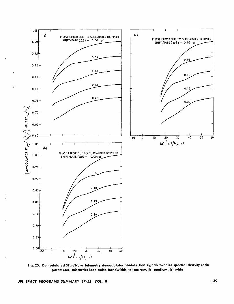
1.05

1.00

O.95

0.90

O.85

0.80

O. 75

Z

0.70

O. 65Z

_0.600

z

"_ 1.05

_ 1.017

O. 95uJ

0.90

(o)

I I I I I

PHASE ERROR DUE TO SUBCARRIER DOPPLER

SHIFT/RATE (AS) : 0.00 rod

0.05

O. 85

0,80

O. 75

O. 70

0.65

0.60-10

Fig. 25.

I

(c)

I

(b)

I ] I I I

I I I l I


SHIFT/RATE (Z_8) = 0.00 rad

I t l I I


SHIFT/RATE ( A8 ) : 0.00 rad

0.10

0.15

0.20

I ] I I t t I-10 0 I0 20 30 40 50

2 x S/N 0,(a') dB

O. 05

0.10

0.15

0.20

t I I I I I0 10 20 30 40 50 60

2 S/NO ' dB(a') ×

Demodulated ST._r/No vs telemetry demodulator predetectlon signal-to-noise spectral density ratio

parameter, subcarrier loop noise bandwidth: (a) narrow, (b) medium, it) wide

6O


2

101

10°

6

4

. I0-I-r

g 6

_ 4

• 2o

. I0-2

Z< 2

,in,

u_ 102

0

>- 6LJ

7

40

2

i01

6

4

10 0

6

4

(a) PHASE ERROR A8 = 0.20rad

0.15

0.10

0.05

1 I I I 1 I

I I I [ I I

(b) PHASE ERROR A8 = 0.20 tad

I

_. WIDE BANDWIDTHi

I

I

0.15

0.10

0.05

MEDIUM BANDWIDTH -

I0 -I I I t i I i

0 10 20 30 40 50 60

2

(a') x /S/N0' dB

7O

Fig. 26. Subcarrier frequency offset vs signal-to-noise

spectral density ratio parameter, subcarrler loop

noise bandwidth: (a] narrow,

(b) medium or wide

0 I I I _" ._ "'T - I I

-4--8-- /

/ ,_' 3D

I ,,_ sY

TSy

PROBABILITY DATA SYMBOL STREAM SWITCHES

ON SUCCESSIVE DIGIT PERIODS0%

-24 _ 50%

_-_ I00%

-28 I l . i I I I I-15 -10 -5 0 5 I0 15 20

STsy/N0, dB

Fig. 27. Telemetry subcarrier demodulator data

suppression factor vs ratio of signal energy

per symbol to noise spectral density

-12

o

-16

-20

I 0°

6

4

2a

z

_ 10 -I

OZO 6

O

2

25

1 I i-- t I I

-

662/ i331/_

I SUBCARRIERT_CKING LOOP_NDWIDTH- NARROW

b = 1/s

10_2 50% PROBABILITY DATA BIT STREAM SWITCHESI I I t 1 I

-10 0 10 20 30 40 50 60

STB/N 0, dB

Fig. 28. Mariner Mars 1969 uncoded telemetry,

telemetry demodulator two-sided closed-loop

noise bandwidth vs ratio of signal energy

per bit to noise spectral density


I|1

0.16

0.12

0.C8

0.04

-4

TI_3 bP'AiTt_,,_'$ SUBCARRIER TRACKING LOOP BANDWIDTH- NARROW

T_ = 1/3

50% PROBABILITY DATA BIT STREAM SWITCHES

I I I. I I I I

0 4 8 _2 16 20 24 28 32

STB/N0, dB

Fig. 29. Mariner Mars 1969 uncoded telemetry, telemetry demodulator rms phase noise error vs

ratio of signal energy per bit to noise spectral density

36

0.95

'_° 0.90

0.85

8 o.8o!

0.751-5

I I I I I I I

/ SUgCARRIER TRACKING LOOP

/ BANDWIDTH - NARROW

r D

TB = 1/350% PROBABILITY DATA BIT STREAM SWITCHES

,_8 _ O. OOrad

5 10 15 20 25 30 35

ST_'_,IO, dg

Fig. 30. Mariner Mars 1969 uncoded telemetry,

demodulation efficiency vs ratio of signal

energy per bit to noise spectral density

From Fig. 25 for ±0 = 0 rad,

demodulated ST,No

ST_input No

= 0.840

Proceeding in this manner, the performance character-

istics shown in Figs. 28, 29, and 30 are obtained foruncoded data rates of 81J_,331/a, 66%, and 270 bits/s.

References

1. Davenport, W. B., "Signal-to-Noise Ratios in Bandpass Limlters,"

1. Appl. Phys., Vol. 24, No. 6, pp. 720--727, June 1953.

2. Tausworthe, R. C., Theory and Practical Design of Phase-Locked

Receivers, VoL I, Technical Report 32-819. Jet Propulsion Lab-

oratory, Pasadena, Calif., Feb. 15, 1966.

8. Jaffe, R. M., and Rechtin, E., "Design and Performance of Phase-

Lock Circuits Capable of Near-Optimum Performance Over a

Wide Range of Input Signals and Noise Levels," IRE Trans.

Info. Theorg, Vol. IT-l, pp. 66--76, Mar. 1955.

4. Golomb, S. W., Baumert, L. D., Easterling, M. F., SUrlier, J'. ].,

and Viterbi, A. 3, Digital Communications. Prentice-Hall, Inc.,

Englewood Cliffs, N.J., 1964.

6. High-Rate Telemetry Project: Subcarrier DemodulatorPerformance, M. H. Brockman

This article provides information on the performance

of the telemetrT subcarrier demodulator which incorpo-

rates a soft bandpass limiter in the subcarrier tracking

loop. Reference material pertaining to the following dis-

cussion is contained in Subsection 5 of this SPS (MMTS:Performance of Subcarrier Demodulator).


For Mariner Mars 1969, the block-coded telemetrydata will have a data rate of 16.2 kbits/s with 6 bits/

word. At minimum operating condition (moc), a 1%

word-error rate is specified which corresponds to an

STJNo (moc) of very nearly +8.0 dB (Ref. 1). Since

10 I

6

Z 100

6

I--

2

10-1-5

1 t I I I I I

_-- = 1/3TSy

SUBCARRIER TRACKING LOOP IANDWIDTH - MEDIUM

DATA RATE: 16.2 kbits/s

6 blts/word

50% PROBABILITY DATA

SYMi_DL STREAM SWITCHES

t J 1 t I t I

0 S 10 15 20 25 30

ST|//N0, dB

Fig. 31. Mariner Mars i969 high-rate block-coded

telemetry, telemetry demodulator two-sidedclosed-loop noise bandwidth vs ratio of

signal energy per bit to noise

spectral density

35

I = 25/6 symbols/bit, and STsr/No = 1/l X STJNo, the

corresponding STsr/No (moc) is -4.8 dB with a symbol

rate of 86.4 ksymbols/s. At mission dp, a 10% bit-error

rate corresponds to an STJNo (dp) of very nearly

-1.0 dB, which provides an STsr/No (dp) of -8.8 dB.

Consider the case at STsy/No (dp), where ro/T_r = 1/3

and there is an assumed 50% probability that the datasymbol stream switches.

STsy- 8.3 dB

No

For 86.4 ksymbols/s,

1Tsy - +49.4 dB/symbol

S- +41.1 dB

• . No

From Fig. 27, (Subsection 5)

(a') _B = - 12.6 dB

S• • (a') z X No - +28.5dB

0.0e

0.06-

0.04-

c

0.02-

-4

I I I I I I I I I

\

\\ r DATA RATE: 16.2 kbits/s

_\ _ . 'D = 1/6 6 blts/word

50% PROBABILITY DATA SYMBOL STREAM SWITCHES

0 4 8 12 16 20 24 28 32

STB/N0, dB

36

Fig. 32. Mariner Mars 1969 high-rate block-coded telemetry, telemetry demodulator rms phase noise error vs

ratio of signal energy per bit to noise spectral density


TII

For operation on medium subcarrier loop bandwidth:

From Fig. 28,

BWscL = 2.18 Hz

From Fig. 24,

a0, = 0.062 rad rms

From Fig. 25c, for ±0 = 0 rad,

demodulated STsrNo

STsrinput No

= 0.938

Continuing in this manner, the performance character-

istics shown in Figs. 31, 32, and 33 are obtained for

?JTsr equal to 1/_and %. The transformation of STsr/No

to the corresponding ST_/No has been made in Figs. 31,

32, and 33 as a convenience in interpreting the resulting

performance.

It should be pointed out that the characteristics dis-cussed above for the block-coded phase-shift key at

16.2 kbits/s and 6 bits/word are based on the assumption

that the data symbol rate and subcarrier frequency are

incoherent (statistically independent). They are, however,coherent in this case with three subcarrier cycles per

symbol period. As a consequence, selection of ro/Tsv

,,.._ 0.115

O.llO

2

0.105

0.100

0.95 -

0.90-

uJ

_ 0.85

-5

l I I 1

SUBCARRIER TRACKING LOOP

BANDWIDTH - MEDIUM

DATA RATE: 16.2 kblts/s

6 bits/word50% PROBABILITY DATA

SYMBOL STREAM SWITCHES

I I I

f A8 = 0.00 r_l0.05

_3 rO ----- srff- -

I I t I I _l I0 5 10 15 20 25 30 35

STB/N0, dB

Fig. 33. Mariner Mars 1969 high-rate block-coded

telemetry, demodulation efficiency vs ratio of

signal energy per bit to noise spectraldensity

will, in all probability, be based on minimizing the phaseerror ±# which results from this coherence, should it be

significant (see SPS 37-51, Vol. II, pp. 136-140). Figure 88illustrates the effect of the phase error ±0 on the demod-

ulation efficiency of the telemetry subcarrier demodulator.

Reference

l. Golomb, S. W., et al., Digital Communications. Prentice-Hall,

Inc., Englewood Cliffs, N.J., 1964.


V. Operations and Systems Data Analysis

11"

A. Ground Communications Facility Operations

1. Flight Project Support, F. e. Bon_,Jr.

a. Pioneer Project. The normal complement of voice

and teletype circuits interconnecting the SFOF and theDSIF stations assigned to track the Pioneer VIIi space-

craft was provided as scheduled. Received dat a were

provided for tracking and data analysis to SFOF users, aswell as to contractor personnel at TRW in Redondo

Beach, California, and to the Ames Research Center at

Palo Alto, California, over discrete voice and teletype

circuits allocated for this purpose. All real-time DSN

communications support was provided in accordance

with existing plans.

Plans are curreritly being developed relative to the

ground communications required for the Pioneer IX mis-sion. Initial indications reveal that this mission will re-

quire communications of a somewhat more complex

nature than previous Pioneer missions, but that the total

communications support required is within the capa-bilities of the DSN/GCF.

b. Mariner V extended mission operations. The DSIF

was scheduled to reacquire the Mariner V spacecraft on

July 22, 1968, and to continue tracking until January 22,

1969. In view of this requirement, total communications

plans were developed and documented for the committed

support. As of this date, the spacecraft has not beenreacquired, but full communications support is available

when needed for telemetry, tracking, and commandactivities.

The operational simplex teletype circuit from theSFOF to Stanford University required by the Mariner V

Extended Mission Operations (MEMO) Project is in-

stalled and operational. The operational simplex teletype

circuits to the University of Iowa and the University ofColorado, both from the SFOF, and a similar circuit to

the Massachusetts Institute of Technology, from Goddard

Space Flight Center, have been installed in accordance

with MEMO requirements.

c. Mariner Mars 1969 Project. Because of the complex

communications requirements established by the Ma1_nerMars 1969 Project and the necessity for initial audio,

teletype, and video configurations in the assigned SFOF

areas, efforts are now underway to define the total

requirements and design the configurations. Subsequent

to such actions, all operational communications plans willbe documented to ensure that the required DSN/GCF

support will be eflqciently provided during the simulation,

launch, and cruise phases of the Mariner Mars 1969

spacecraft.

t|

!


I!11

d. Biosatelllte Project. Based on preliminary informa-

tion, communications plans are being developed to

receive high-speed data from the Space Tracking and

Data Acquisition Network (STADA.N) over DSN/GCF

circuits at the SFOF for further processing in SFOF

computer facilities. The original proposals for this sup-

port specify that two 30-day missions are contemplatedand that data flow will occur for approximately 10 h

each day during the scheduled missions for March and

September 1969.

B. DSN Systems Data Analysis

1. Computation of the Normal Matrix far DiscreteMultidimensional Approximations, A. c. Johnson

a. Introduction. Occasionally, it is desirable to obtain

a multidimensional linear least-squares polynomial ap-

proximation to a function whose value is known only for

a discrete or finite set of points. This problem arises, for

example, when obtaining estimates of antenna pointingerrors.

In this connection, the following questions have been

asked: "How does one form the normal equations or the

normal matrix when there are two or more variables?"

and, "Precisely how does the number of data points used

enter into the approximation problem?"

When considering two or more variables, the formu-lation of the normal matrix, while not difficult, is quite

tedious and is generally known to the mathematician

only. The number of data points used is directly related

to the approximation problem, and the answers can be

deduced from the general theory of approximations on

normed linear spaces. It will be noted that the results

presented can easily be extended to the case of anynumber of variables and is not limited to polynomial

approximations. This method is a more general and

straightforward approach to the formulation and com-

putation of the normal matrix corresponding to discrete

multidimensional approximations.

b. Abstract [ormulation of the discrete linear approxi-

mation problem. Let V denote the linear space of all

bounded functions [(x, y) defined on a given region D in

two-space.

D=(x,y), a_-_x_b, cGy<<_d

Let (xi, y_)--i = 0, 1, "- N; i = 0, 1, -.- M--be any set of

points D' in D.

D' = (xi, y_), (xl, y_) • D; i = 0, 1, "" N; i = 0, 1, "-" M

Now introduce an "equivalence" relation on V, fl _ f.-,, if,

and only if,

_1 (Xi, Yj) = f2 (Xi, Yj), (xi, y_) • D'

Let V denote the family of all equivalence classes offunctions in V. If a is a constant and ['• V, then by a7 is

meant the equivalence class of af, denoted by a['-_With

this definition of scalar product, it is easy to prove that

is a linear space. Moreover, the dimension of V is finite

and may be deduced in the following way.

The function f • V is equivalent to the function gl where

gs(x,y) =/(x, y), (x, y) • D'0, otherwise

Let

1,

y) =( O,

(x, y) = (xi, y_), i = 0, 1, "'" N

i=O, 1,...,Motherwise

Then the (N + 1) (M + 1) vectors, "_j(x, y), are linearly

independent and every gl is a linear combination of the

M N

i=o J=0

Thus, the dimension of V is (N + 1) (M + 1) [so that V is

algebraically equivalent to the vector space of (N + 1)

(M + 1)-tuples].

Next, define an "inner" product of two vectors [-_ and

in V by means of the function

N M

<_,[_> = _ _=o[_(x_,y_)f..,(xi, y,) (1)

The following relations are easily verified directly fromthe definitions

<a_, b_,> = ab <_,-[_> , aand b are constants

(2)

(3)

<7"1, fx> = 0, if, and only if, f-1 = (4)


i.e., fl is equivalent to the function which is identically

zero on D. The Relations (2), (3), and (4) show that the

inner product defined here is a positive definite, symmetricbilinear function and hence can be used to define a

"suitable" norm on V. (By a "suitable" norm or "distance"

function, one usually means a real-valued function on× V which satisfies our intuitive notions of distances

between points in space. For example, the distance be-

tween distinct_points should be positive.) By definition,the "norm" of f e V, or the "distance" of ]. from O e V, isdefined as

and the "distance" of f'l from f., is given by the equation

{ 1II - I1= (x,,yj)- f,(x,,y,/li=o J=0

Thus, one can formulate the discrete linear approxima-tion problem for functions or vectors f, which are elements

of a finite dimensional normed linear space _. Note thatw

an approximation to f E V is interpreted as an approxi-

mation to a family of functions; namely, that family

which takes on the values f(x, y) whenever (x, y) e D'.

One can now apply the following well-known theorem

concerning (least-squares) approximations on normedlinear spaces.

Theorem. If R is a subspace of a finite dimensional

normed linear space _ and if ]'is any vector in V- R, thenthere exists a unique vector fo E R such that

FlTo-ftl < I!?-_II (6)

m

for every vector _ e R -- [fo]. Moreover, if the "norm" on

V is "induced" by an inner product then

<T- f=,:> =o (7)m

for every _ _ R.

Relation (7) enables one to determine explicitly that

vector fo deviates least from a given f. For ifFk, k = 0, 1,... K

is a basis for R, then since fo E R, there exist constants aksuch that

K

]'o(x,y) = _ a_-_(_,y) (8)k=0

Moreover, since _k _ R, it follows from Relation (7) that

<f---/o,¥k) = O, k=O, 1,"'K

or

=\J, /, k =0,1,...K (9)

On substituting in Eqs. (9) the value of f-o in Eqs. (8),

K

at<'rt, Tk>=<f, Fk>, k=O, 1,...Kt=0

(10)

Equations (10) are the "normal" equations.

c. Applications to multidimensional least-squares poly-

nomial approximations. Let R be that linear subspace of

V Consisting of all polynomials of the form

r q

t=o q=0

where T < N, Q < M, and (N + 1) (M + 1) is the dimen-

sion of the space V defined above. Since T < N and

Q < M, it follows that if P_, P2 • R, then P_ _-_ P2, if, and

only if, e_ (x, y) -_ Pz (x, y), (x, y) _ D. Thus, in the state-ment of the above theorem, R may be replaced by R, and

hence there is only_one polynomial which deviates theleast from a given f _ V.

It is obvious that the functions

xtyq, t -= O, 1, " " T, q =0,1,..'Q

form a basis for R. Let f-be a given function in V withvalues

f(xi, y_), (xl, yj) _ D'

Then the normal equations corresponding to a least-

squares polynomial approximation to f-(x, y), or equiva-

lently to f(x, y), (x, y) e D', are by Relation (7) the following:

t=o q=0

r=O, 1,..- T;l =O, 1,... T (11)

=


i|1

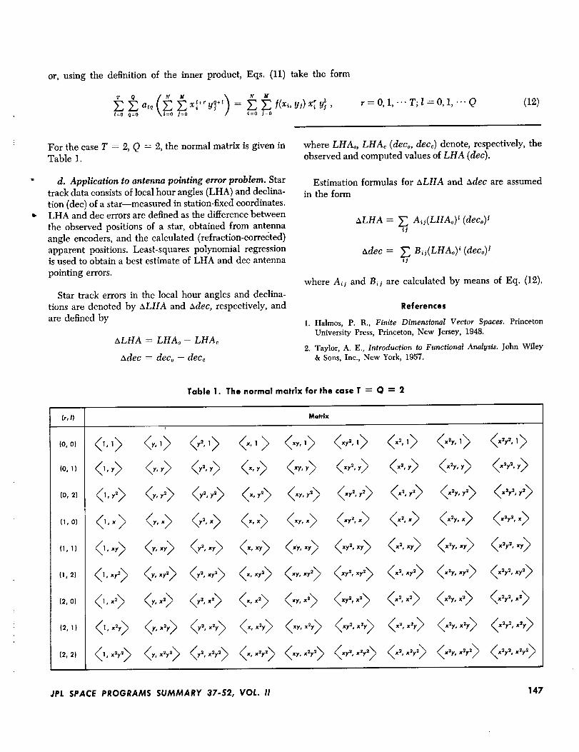
or, using the definition of the inner product, Eqs. (11) take the form

O t+r +l r__, atq x, y_ = 2 _-, [(x" y') x_ Y ,

t=o q=o i=o 1=o i=0 I=o

r=O, 1,... T;l=O, 1,'"Q (12)

For the case T = 2, Q = 2, the normal matrix is given inTable 1.

d. Application to antenna pointing error problem. Star

track data consists of local hour angles (LHA) and declina-

tion (dec) of a star--measured in station-fixed coordinates.LHA and dec errors are defined as the difference between

the observed positions of a star, obtained from antennaangle encoders, and the calculated (refraction-corrected)

apparent positions. Least-squares polynomial regressionis used to obtain a best estimate of LHA and dec antenna

pointing errors.

Star track errors in the local hour angles and declina-

tions are denoted by ±LHA and adec, respectively, and

are defined by

LxLHA = LHAo - LHAc

Adec = dec° - decc

where LHAo, LHAc (dec°, decc) denote, respectively, the

observed and computed values of LHA (dec).

Estimation formulas for hLHA and Adec are assumed

in the form

±LHA = _ A,_(LHAo)' (deco) jU

adec = _, B,j(LHAo) i (deco) siI

where Aij and B_ i are calculated by means of Eq. (12).

References

1. Halmos, P. R., Finite Dimensional Vector Spaces. PrincetonUniversity Press, Princeton, New Jersey, 1948.

2. Taylor, A. E., Introduction to Functional Analysis. John Wiley& Sons, Inc., New York, 1957.

Table 1. The normal matrix for the case T = Q = 2

{r,I) Matrix

,o.0, (,.,)

..,. (,,x,)


2. AnImprovedMethodfor RangeDelayCalibration,S. C. Ward and F. Borncamp

a. Introduction. Any RF ranging system determines

range by measuring propagation (delay) time to the target

and back. This propagation time includes delays caused

by equipment and cables as well as those caused by the

round-trip signal transit time. To make the system accu-

rate, these nonspace-caused delays must be found and

subtracted from the range. The JPL range-measuring

system con.verts accumulated phase of a pseudonoise

coded phase-modulated carrier to the spacecraft and backinto range, effectively measuring range at lunar distances

to better than 15-m accuracy.

This article suggests a revised method of measuring

the portion of the range measurement caused by delays

in the ground station equipment. The new method re-

quires significantly less man-hours to perform the cali-

bration, and it also may be used at all stations, includingthe Mars DSS. Tests were conducted at the Pioneer DSS

to compare the new method with the old, and the results

show the two methods to be of equivalent accuracy.

b. The present method. The system presently used by

the DSIF is the "big black box" concept (Fig. 1). Basically,

it involves ranging over a "known" distance with overall

ground equipment, including the tracking antenna de-

fined as a large black box. All delays outside the box are

accurately known; thus leaving the difference between

measured range and the actual range due only to the box.

Although this method of calibration is effective and

reasonably accurate, it has the following faults:

(1) A first-order survey is necessary, and the survey iscomplicated by the fact that it must be referenced

to the RF axis of the tracking antenna--a point

that is not readily accessible to the surveyor.

(2) The tracking antenna must be deflected to the

collimation tower, thus preventing calibration of

the system with the antenna at or near the positions

used during spacecraft tracking.

(3) To ensure that the calibration is performed at the

same power levels (both uplink and downlink) as

those expected during a spacecraft track, a tech-

nician must go to the spacecraft simulating equip-ment at the collimation tower to activate it and to

adjust the backside attenuators that control down-

link power. This becomes a problem at stationswhere the collimation tower is difficult to reach.

At two DSIF stations, a team of two men must be

sent; during inclement weather, the collimationtower cannot be reached at all.

(4) Stations using 210-ft-diam antennas cannot be cali-

brated because there is no collimation tower. (The

1

I 85-fl

[BIGBLACK BOX _ DISH ._,J _"1

l_

IITRANSMITTERI

tRANGE

SUBSYSTEM RECEIVER

i JI J

1 m; (AVERAGE)

100-200 fl

COLLIMATION

I TOWER

Fig. 1. Present black box method for range delay calibration

VARIABLE

ATTENUATOR

(FRONTSIDE)

ZERO DELAY

IRA NS LATOR

t81-MHz

OSCILLATOR

VARIABLE

ATTENUATOR

(BACKSIDE)

It-


IIi

required tower would have to be 11 mi in height

and located 26 mi away.)

Also contributing to the uncertainties of this method,

or limiting the flexibility, are the following conditions:

(1) Because the collimation tower antenna is from 100

to 200 ft above ground, it is difficult to measure

accurately its propagation velocity. It, therefore,

must be estimated from the manufacturer's speci-fications.

(2) The propagation velocity calibration of the 100 to

250 ft of coaxial cable varies with temperature,

condition of the dielectric (moisture, breaks), and

unverified changes in the cable or sections thereof.

To prevent damage to the translator diode, front-

side attenuators are required at uplink powerabove 100 W. The present off-the-shelf attenuators

are only good to 10 kW and, therefore, cannot be

used for calibrating at 20 kW.

c. New method. The revised method is basically the

same as the big black box method, except the turn-

around translator is mounted on the edge of the 85-ft-

diam dish. The location was chosen to minimize possible

multipath effects off the quadripod. In addition, it was

desirable to find a mounting point which would not

involve using any of the present mesh surface of the dish.

The location and suggested method of mounting is shown

in Fig. 2.

The station measured the delay, using the same tech-

niques as if they were ranging to the collimation tower.

Only a small known figure is necessary to measure back

to the reference point at the intersection of the RF axisand the centerline of the declination shaft. For the test, a

cable was run from the translator about 100 ft to the

variable attenuators and oscillator portion of the trans-

lator. Thus, only the antenna and diode were mounted

on the dish edge. This permitted the operator to vary the

downlink signal level as requested from the control room.

This proposed range-delay calibration technique elim-

inates the need for a survey and aII the uncertainties andman-hours associated with the collimation-tower tech-

nique. The off-beam location has sufficient inherent

attenuation (72 dB) to negate the need for frontside

attenuators. Because the system can be calibrated with

the tracking antenna in track position, all the uncertain-

ties due to structural deflections and changes in the

cable wrap-up are removed or greatly lessened.

Implementation of the following changes will further

lessen required manpower and shorten the calibration

procedure:

(1) Use a coherent (181-MHz) frequency for mixing at

the diode, thus providing a zero doppler signal tothe range subsystem. There are methods which can

be used if an RF doppler signal is non-zero, butthey can lead to errors and are somewhat incon-

venient for the operator. The required signal is

TRANSMITTER

i 30--210 ft

' DISH"

[ RECEIVER

RANGE I_ JSUBSYSTEM

II 181 -MHzOSCILLATOR

181-MHz I

OSCILLATOR '

AT 10 dBm

I

Fig. 2. Proposed method for range delay calibration


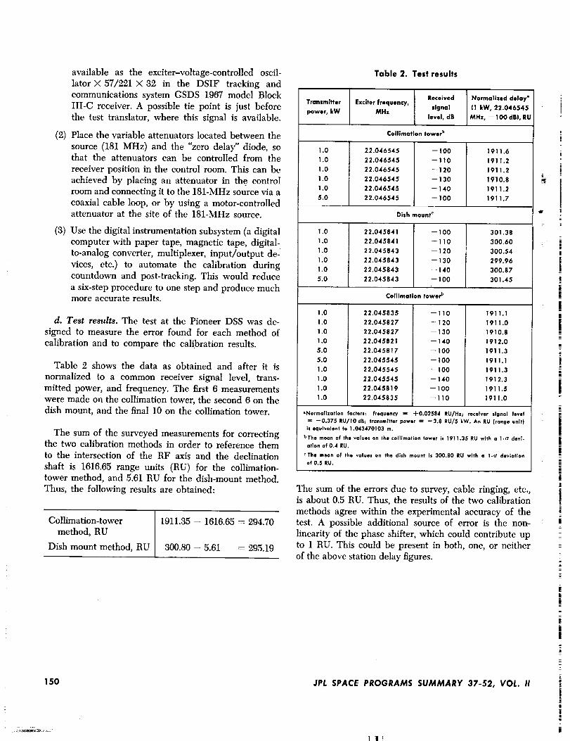
(2)

(3)

available as the exciter-voltage-controlled oscil-

lator × 57/221 × 32 in the DSIF tracking and

communications system GSDS 1967 model Block

III-C receiver. A possible tie point is just beforethe test translator, where this signal is available.

Place the variable attenuators located between the

source (181 MHz) and the "zero delay" diode, sothat the attenuators can be controlled from the

receiver position in the control room. This can be

achieved by placing an attenuator in the controlroom and connecting it to the 181-MHz source via a

coaxial cable loop, or by using a motor-controlledattenuator at the site of the 181-MHz source.

Use the digital instrumentation subsystem (a digital

computer with paper tape, magnetic tape, digital-

to-analog converter, multip/exer, input/output des

vices, ete.) to automate the calibration during

countdown and post-tracking. This would reduce

a six-step procedure to one step and produce muchmore accurate results.

d. Test results. The test at the Pioneer DSS was de-

signed to measure the error found for each method of

calibration and to compare the calibration results.

Table 2 shows the data as obtained and after it is

normalized to a common receiver signal level, trans-

mitted power, and frequency. The first 6 measurements

were made on the collimation tower, the second 6 on thedish mount, and the final 10 on the collimation tower.

The sum of the surveyed measurements for correctingthe two calibration methods in order to reference them

to the intersection of the RF axis and the declination

shaft is 1616.65 range units (RU) for the collimation-tower method, and 5.61 RU for the dish-mount method.

Thus, the following results are obtained:

Collimation-tower

method, RU

Dish mount method, RU

1911.35 - 1616.65 = 294.70

300.80 - 5.61 = 295.19

150

Table 2. Test results

Received Normalized delay"Transmitter Exciter frequency,

power, kW MHz signal (I kW, 22.046545level, dB MHz, -- I00 dB), RU

Collimation tower b

1.0

1.0

1.0

1.0

1.0

5.0

22.046545

22.046545

22.046545

22.046545

22.046545

22.046545

-- 100

--110

--120

--130

--140

-- 100

1911.6

1911.2

1911.2

1910.8

1911,2

1911.7

1.0

1.0

1.0

1.0

1.0

5.0

Dish mount _

22.045841 --100

22.045841 -- 110

22.045843 --120

22.045843 --130

22.045843 -- 140

22.045843 --100

Collimation tower b

301.38

300.60

300.54

299.96

300.87

301.45

1.0

1.0

1.0

1.0

5.0

5.0

1.0

1.0

1.0

1.0

22.045835

22.045827

22.045827

22.045821

22.045817

22.045545

22.045545

22.045545

22.045819

22.045835

--110

--120

--130

--140

-- 100

-- 100

-- 100

--140

-- 100

--110

1911.1

1911.0

1910.8

1912.0

1911.3

1911.1

1911.3

1912.3

1911.5

1911.0

"Normal;zation factors: frequency _ +0.02584 RU/Hz; receiver signal level

== --0.375 RU/IO dB; transmitter power = --3.8 RU/5 kW. An RU [range un;t)is equivalent to 1.043470103 m.

bThe mean of the values on the collimation tower is 1911.35 RU with a 1-tr devl-

ation of 0.4 RU.

The mean of the valuel an the dish mount is 300.80 RU wlth a 1.o" deviationof 0.5 RU.

The sum of the errors due to survey, cable ringing, etc.,

is about 0.5 RU. Thus, the results of the two calibration

methods agree within the experimental accuracy of thetest. A possible additional source of error is the non-

linearity of the phase shifter, which could contribute up

to 1 RU. This could be present in both, one, or neitherof the above station delay figures.


1|[

VI. Technical Facilities

A. Antennas

1. Woomera DSS Antenna Mechanical Upgrade,W. Kissane and M. Kron

The mechanical upgrade of the Woomera DSS antenna

structure and mechanical equipment (SPS 87-51, Vol. II,

p. 174) is continuing. The hour-angle and declination

gear segments were removed, and stiffening shear plateswere welded to the rim of the hour-angle wheel to help

maintain the shape of the wheel after the structure was

loaded with counterweight. Also, several main members

supporting the counterweight box were sequentially re-

placed with new members whose section properties

reflect an increase in strength of 200% to 400%. The

combined effects of the shear plates, the stronger mem-

bers, and an increased number of fasteners at each joint

connection have greatly reduced the deflection character-

istics of the hour-angle wheel. As an adjunct to the

replacement by stronger members, all joint fasteners

were replaced with high-strength interference bolts to

avoid slippage under cyclic loading conditions.

The entire structure was loaded with all of its operat-

ing dead loads, including the feed cone, and all of the

gear segments on both the hour-angle and declinationwheel were reset. The total indicated runout of the gear

teeth was checked and adjusted such that the eccentricity

error of the wheel meets specification requirements. The

clearance between the wheel rim and the back surface

of each gear segment is being filled with molten Kirksite.The new drive skids are being given a final adjustment

for gear running clearances.

Installation of the new cable wrapup systems, de-

veloped on a prototype basis at the Goldstone DSCC,and associated cable tray runs were completed, as were

preliminary measurements of the reflector surface and

installation of the primary datum plane targets. Presently

the initial data from theodolite readings are being re-

duced to determine the shim sizes to be used for the final

dish setting.

Final detail work on the structure is under way con-

currently with a review of the complete upgrade effort.

2. Echo DSS Antenna Mechanical Upgrade,

R. McKee and J. Carlucci

ModificatiOns of the 85-ft-diam HA/dec antenna at the

Echo DSS began in early February 1968. Previous report-

ing on these modifications appeared in SPS 87-51, Vol. II,

pp. 171-178.

Rebolting of the pedestal, hour angle wheel, declination

wheel, and box girder has been completed. Addition of

welded gussets in the box girder area is also complete.


Old surface panels and attachment hardware have beenremoved, and setting of new panel attachment hardware

is nearly complete. Installation of new high-performance

S-band surface panels has begun with the installation of

the inner row of panels and positioning of panels spanningtwo main rib trusses to the outer edge of the dish structure.

The upper and lower electronics rooms are nearly

complete, with some insulated wall panels yet to beinstalled.

New hour angle and declination cable wrap-ups have

been installed; installation of cable trays has begun on

the pedestal structure.

New declination drives have been installed and roughset.

The declination gear has been reset and is ready for

the final runout check and pouring of Kirksite (low-

temperature metal shim between the gear segments and

the wheel flange to create a solid metal shim). Resetting

of the hour angle gear is in progress.

B. Buildings

1. SFOF Mariner Mars 1969 Mission Support Area,ttJI. Salem

The Mariner Mars 1969 mission support area in the

SFOF has been functionally specified, and a configura-

tion determined. Detail designs for the necessary wall

modifications and the electrical distribution system within

the mission support area have been completed. As speci-

fied in the NASA Support Instrumentation Requirements

Document, the Mariner Mars 1969 mission support area

will contain the following distinct sub-areas: mission

director's room, mission control room, observation room,

spacecraft performance analysis area, conference room

(existing), space science analysis area, principal investi-

gator's area, and flight path analysis area (existing).

The physical arrangement of control and analysis areas

is based upon previous Mariner Project operations

wherein the mission control room was placed contiguous

to the spacecraft analysis areas to improve interactionand communication. The mission control room will fea-

ture one of the round, six-man conference consoles used

very successfully for the Pioneer VIII launch operations

and the Surveyor V, VI, and VII mission operations. The

mission director and his staff will be positioned such that

they can observe all operations when necessary but can

remain separated from the operations when desired. Anobservation room will permit visitors a direct view of all

mission operations from outside the immediate analysisareas.

The spacecraft performance analysis area will house

the spacecraft performance analysis and command direc-tor, an assistant director to head each of the two space-

craft teams, a test director and recorder for each team,

and 20 analysts. The data display equipment will be that

utilized for all mission operations conducted from the

SFOF since the Mariner IV mission operations in 1964.Communications within the area, as well as with the

remainder of the mission operations team, will be accom-

plished through the use of the operational voice commu-

nications subsystem networks. The television subsystem

will be utilized for time display and dissemination of

updated sequence-of-events information, as well as dis-

play of many individual elements of teletype information.

Analysts will be seated at desks or tables. The area

director, his deputy, and an assistant will utilize the area

director's consoles, which provide increased capabilityin both the television and voice communications sub-

systems. The height of these consoles is being lowered

approximately 8 in., and their top is being sloped to pro-

vide a significant improvement in forward visibility for

the operators.

C. Utilities

1. Goldstone DSCC Communications Switching

Center, B.c. Bridges

To standardize communications equipment configura-

tions throughout the DSN, it was decided to reconfigure

the DSS communications switching centers. The recon-

figuration of the center serving the entire Goldstone

DSCC (located at the Echo DSS) is expected to be com-

pleted in September; that of the centers at the Woomera,Johannesburg, and Cebreros DSSs is scheduled for com-

pletion by January. The consolidation of equipment

(tactical intercom, teletype, high-speed data, stations

communications control group, and microwave) in one

centrally located area--the primary goal of the recon-

figuration effort--will result in fewer operational per-

sonnel being required; i.e., only one technician and one

teletype operator will be required each schedule shift.

The interstation microwave switching equipment at

the Goldstone DSCC center is shown in Fig.. la. All

communications coming from the Pioneer, Echo, Venus,

and Mars DSSs are switched through to JPL. Conversely,

!


lit

1

|

Fig. I. Goldstone DSCC communications switching center equipment: Ca) interstation microwave switching

equipment, (b) Western Union microwave and multiplex equipment, (c) stations

communications control group, (d) main distributing frame


all communications coming from JPL by Western Union

microwave (most telephone communications and voice/

data) are switched, or patched, to the appropriate DSS.

The microwave and multiplex equipment leased from

Western Union is shown in Fig. lb.

Four bays of equipment, called the stations communi-

cations control group (Fig. lc), handles all routing of

voice/data, as well as teletype switching, at the Gold-

stone DSCC center. The Woomera, Johannesburg, and

Cebreros DSS centers will require only three such bays:

an attitude of 91 deg from vertical and withstand accel-

eration rates of 8 deg/s in azimuth and 2 deg/s in eleva-

tion, an air-conditioner of special design and constructionwas required.

The 7.5-ton air-conditioner, as shown in Fig. 2, was

designed as three units: two heat exchangers mounted

in the dish structure, and one chiller (with compressQr) i

mounted below the alidade in a structural area that :-:

rotates in azimuth only. _Fhe total load is 58,162 Btu. _ iInstallation, checkout, and calibration of the unit have i

two for teletype and oiae for voice/data. High-speed data been completed.equipment will be provided at these centers, but the

Goldstone DSCC center does not require it. _

All land-line communications (e.g., paging, local, tele-

phone, and teletype) are interconnected through a maindistributing frame (Fig. ld). The telephone central-

office equipment provides all telephone communicationsfor the Goldstone DSCC and all trunk lines to and from

JPL and Barstow. During relocation of the equipment,

200 lines were added, increasing the central-office capa-bility to 500 lines. The central office and all telephone

instruments at the Goldstone DSCC are JPL-owned,

whereas the Woomera, Johannesburg, and Cebreros DSSs

are served by local telephone companies.

2. Air-Conditioner for Venus DSS 400-kW-Transmitter

Antenna, j Carlu¢¢i

Operation of the modified Venus DSS 85-ft az-el

400-kW-transmitter antenna requires temperatures be-tween 60 and 85°F, with only -+-5°F variation from one

level over a 24-h period, and humidity of not more than

50% in the electronics room and cassegrain cone area.

An inherent problem with chiller compressor design isthe sensitivity of such compressors to attitude. Since a

unit for this application would have to operate within

[] i¸¸

E

Fig. 2. Air-conditioner for Venus DSS

400-kW-transmitter antenna

!


f the deep space network

Documents