Eye Tracker Accuracy:Quantitative Evaluation of the Invisible Eye Center Location

Stephan Wydera) and Philippe C. Cattinb)

Department of Biomedical Engineering, University of Basel, Allschwil, Switzerland

(Dated: May 23, 2017)

Purpose. We present a new method to evaluate the accuracy of an eye tracker basedeye localization system. Measuring the accuracy of an eye tracker’s primary intention, theestimated point of gaze, is usually done with volunteers and a set of fixation points used asground truth. However, verifying the accuracy of the location estimate of a volunteer’s eyecenter in 3D space is not easily possible. This is because the eye center is an intangible pointhidden by the iris.Methods. We evaluate the eye location accuracy by using an eye phantom instead of

eyes of volunteers. For this, we developed a testing stage with a realistic artificial eye anda corresponding kinematic model, which we trained with µCT data. This enables us toprecisely evaluate the eye location estimate of an eye tracker.Results. We show that the proposed testing stage with the corresponding kinematic

model is suitable for such a validation. Further, we evaluate a particular eye tracker basednavigation system and show that this system is able to successfully determine the eye centerwith sub-millimeter accuracy.Conclusions. We show the suitability of the evaluated eye tracker for eye interventions,

using the proposed testing stage and the corresponding kinematic model. The results furtherenable specific enhancement of the navigation system to potentially get even better results.

I. INTRODUCTION

Eye tracking devices, also known as eye- or gaze track-ers are used to monitor eye movement. An eye trackeris usually used to determine a person’s point of gaze. Inmarket research, for instance, a wearable, video basedeye tracking system can be used to uncover which prod-uct on which shelf is attracted by a test person. Cer-tainly, there exist other constructions of eye trackers (e.g.desktop or embedded devices) and many other eye track-ing applications (e.g. in usability testing or in automo-tive industry)1,2. Different physical principles might bebehind an eye tracker, depending on the application3.Video based eye trackers are the most widely used de-vices, because of their simplicity and the wide applica-bility.

In recent research, eye trackers are also used in naviga-tion systems for computer assisted eye interventions4–6.In these cases, the eye tracker is used to estimate the3D-location of the patient’s eye, that is the eye centerand orientation. We define the eye center as the centerof corneal curvature. This can be useful to align an eyefor an ophthalmic examination or treatment. Further-more, the point of gaze, estimated by the eye tracker, isautomatically monitored to interrupt an examination ortreatment in case of sudden eye motion.

Using an eye tracker for medical interventions demandshigh system accuracy. This may decide between successor failure of an intervention because of the close proximityof critical structures within the eye. For instance, an eyelocalization accuracy below 1 mm is required, when aneye tracker is used to target intraocular tumors.

The demand for accurate eye tracking systems alsoraises the need for reliable accuracy measurement meth-ods. Accuracy measurements are crucial for the develop-ment of an eye tracking system and also for the perfor-mance specification of the device.

Conventionally, eye tracker accuracy is evaluated withvolunteers, who have to focus on certain fixation pointslocated at well-known positions. The accuracy is thengiven by the deviations between the true fixation point lo-cations and the point of gaze estimates of the eye tracker.As straightforward as this evaluation can be performedon the one hand, as difficult it is to see what parts of thesystem contribute to a certain error on the other hand.Testing this way does not enable us validating the ac-curacy of an intermediate product of the eye trackingpipeline, as for instance the eye center location. Fur-thermore, this validation method obviously depends onthe cooperation of the volunteers. Hence, measuring theaccuracy with an eye phantom seems to be the ideal com-plement for a thorough eye tracker evaluation.

Already Via et al.4 used an eye phantom to asses theaccuracy of an eye tracking system. However, detailsabout the exact procedure remain partially unclear. Fur-thermore, it is not clear how realistic their eye phantomis. Also Swirski and Dodgson recognized the lack of acomprehensive evaluation method to test and improvethe individual parts of an eye tracking system. Theypropose completely synthetic eye data7 for accuracy andprecision evaluation of eye tracking algorithms.

Compared to Via et al.4, we build up our ground truthdata using µCT-measurements to get highly accurate ab-

arX

iv:1

705.

0758

9v1

[cs

.HC

] 2

2 M

ay 2

017

2

Eye tracker

Testing stage

MirrorsCamera & Lens

CorneaCenter of corneal curvatureEyeball

Eye model

Linear stagesRotation stageGoniometer

DOF Microstages

Figure 1: Eye tracker and testing stage (topdown view)

solute eye center locations. In contrast to Swirski andDodgson7, we do not only evaluate the algorithm, butwe validate the complete eye tracking system, includ-ing the whole optical path and the external referencingto a medical device. The evaluation of such an eye lo-calization system involving eye tracker hardware and itsenvironment cannot be done with rendered eye images.Neither can it be done with volunteer tests, because it isnot possible to accurately measure the 3D location of avolunteers invisible eye center.

Accurate ground truth data is required for the accu-racy evaluation of an eye localization system. We pro-pose a procedure to fill this gap by providing accurate3D-locations of the invisible and intangible eye center.

The basis is formed by a testing stage with four de-grees of freedom (4 DOF), a mounted artificial glass eye,and an attached, black and white checkerboard patternfor external referencing. The testing stage enables us tomove the whole eye forth and back and sidewards (by twolinear stages). Additionally, the testing stage enables usto rotate the eye around two axes (by a rotation stage anda goniometer), in order to simulate an arbitrary line ofsight. We built the testing stage and trained the parame-ters of its kinematic model with µCT-data (i.e. high pre-cision 3D volumetric data) acquired of the testing stagein several different configurations (i.e. eye positions andorientations). The µCT-data provides us with accurateinformation about the location and the geometry of theeye and the checkerboard. Figure 1 illustrates the twoinvolved parts, the eye tracker we want to evaluate andthe proposed testing stage to accomplish the evaluation.

Having the testing stage ready and the kinematicmodel trained, we position and orient the artificial eye inknown locations and compare this against the eye centerlocations predicted by the eye tracker. The eye center lo-cations are given by the centers of corneal curvature (i.e.center of a cornea best fit sphere). The trained kinematicmodel provides us with exactly the same point in a com-mon coordinate system (CS), which is also accessible bythe eye tracker. This enables us to compare the eye lo-cation estimates of the eye tracker with the ground truthdata, given by the testing stage model.

Eyeball

Cornea

Lens

Center of corneal curvatureand nodal point of the eye zc

Center of rotation ze

Geometrical axis

Visual axis

Fovea

Point of gaze

Figure 2: Typical eye model used by eye trackers

With the proposed testing stage, it is possible to quan-titatively evaluate the performance of any 3D modelbased eye tracker. Using this method, we show that aparticular eye tracking system6 estimates the eye centerlocation with sub-millimeter accuracy.

We describe in the following sections our proposedmethod for the accuracy evaluation and the resultsachieved when testing a particular eye tracker6.

II. METHODS

We propose a custom-built hardware testing stage andan appropriate kinematic model with its calibration, toevaluate the accuracy of the center location of the cornealcurvature, estimated by an eye tracker. This section con-sists of three parts. First, we give an insight into a typicaleye tracking model based on 3D ray tracing. Second, wepresent the testing stage hardware with its components.The testing stage hardware enables us to position and ori-ent the embedded artificial eye such that the eye trackercan perform its intended measurements. The testingstage hardware basically replaces the testing volunteer,with the advantage of having the exact position of the eye(i.e. ground truth). Third, we present the correspondingtesting stage model, which we parametrize, train and val-idate with µCT data. The kinematic model enables us todetermine the exact glass eye position in every possibletesting stage configuration with sub-millimeter accuracy.

Consequently, this enables us to test an eye trackeron the artificial eye prothesis with several different eyepositions and orientations. The 3D eye location estimateof the eye tracker can then be compared to the groundtruth data of the testing stage model, which is configuredaccording the status of the testing stage.

II.A. Eye Tracker Model

The complexity of existing eye tracking models vary.The eye is often modeled with two spheres. Figure 2 illus-trates such a typical eye model. One sphere representsthe eyeball, its center consequently corresponds to therotation center of the eye. The second sphere, the spherecap respectively, represents the cornea. The center of

3

~x(CSlin2)~x(CSlin2)

~x(CSlin1)~x(CSlin1)

~x(CSgon)~x(CSgon)

(a) Top-down view

~x(CSrot)~x(CSrot)

CScbCScb

yyxx

(b) Bird’s-eye view

Figure 3: Testing stage with the glass eye, its holderwith the checkerboard and the microstages

the corneal curvature corresponds to the nodal point ofthe eye, where the optical rays cross, before they hit theretina8.

The two sphere centers define the geometrical axis ofthe eye. Hence, the orientation of an eye in space can bedetermined by the geometrical axis. The location of theeye (i.e. eye center) is given by the center of the cornealcurvature, which lies on the mentioned, geometrical axisand is an integral part of most of the 3D model basedeye trackers.

The fovea (point of sharpest vision) is located on theretina (backside of the eyeball) but is not in line withthe geometrical axis. A point we focus on with our eyegets imaged on the fovea. That is why also the visualaxis plays an important role in such a model. The visualaxis connects the fovea with the nodal point of the eyeand the point of gaze. The angle between visual axis andgeometrical axis has to be calibrated per patient.

The eye tracker5,6 which we test with the proposedtesting stage is based on the model of E. D. Guestrinand M. Eizenman8.

II.B. Testing Stage Hardware

The testing stage we developed consists of a trans-lation stage with two axes with parameters P1 and P2

(OptoSigma TADC-652WS25-M6 ), a goniometer stagewith parameter P3 (OptoSigma GOH-65A50-M6 ), anda rotation stage with parameter P4 (OptoSigma KSW-656-M6 ). The variables P1, P2, P3, and P4 represent thevalues, which are set for the corresponding microstages.The linear stages have a vernier scale included enablingto measure with a precision of 10µm. The rotation stageand goniometer also contain a vernier scale enabling usto measure with a precision of angular minutes. To sim-ulate the human eye, we use a handcrafted eye prosthe-sis made from glass by the Swiss Institute For ArtificialEyes, Lucerne, Switzerland. To interface the artificial eyewith the stages we designed a rigid and robust eye holder.Since the eye prosthesis does a priori not have an exactly

Microstage parametersP1, P2, P3, P4

Testing stagehardware

Eye tracker

Testing stage model

zc, ze = f(θ, P1, P2, P3, P4)

Comparison

adjust microstages

feed model

measure

estimated z?c , z?e

true zc, ze

Figure 4: Concept of testing stage: Comparison of theeye center location z?c estimated by the eye tracker with

the ground truth zc

known geometry, we made a 3D scan of it with a µCTdevice (GE phoenix nanotom m). We segmented the sur-face of the eye with Fiji, an image processing package9.We afterwards used Blender, an open source 3D creationsuite (http://www.blender.org), to design a holder accu-rately interfacing the eye with the stages. The holder ad-ditionally contains a black and white checkerboard stuckon its side. The checkerboard is printed with an off-the-shelf laser printer, which contains toner visible in theµCT. The stages are serially mounted and on top ofthem is the eye holder, which was printed on a StratasysFortus 250mc 3D printer. The testing stage is shown inFigure 3.

II.C. Testing Stage Kinematic Model

The aim of the kinematic model is to determine theexact center location of the corneal curvature zc for acertain testing stage configuration (P1, P2, P3, P4) and totransform the coordinates to a common coordinate sys-tem.

The internal model parameters θ, that have to betrained, basically consist of six right-handed coordinatesystems (CS): CSvol is the common CS for all µCT -volumes, CSlin1, CSlin2, CSgon, and CSrot correspond totheir appropriate microstage and CScb is the checker-board CS. CSvol can be seen as the CS for model inputdata, whereas CScb is the CS for the output data. CScb

is accessible by the eye tracker and the testing stage. Ad-ditionally, θ contains zc and ze, the center locations andthe radii of the cornea and the eyeball, yet unaffected byP1, P2, P3, P4 (neutral position).

Figure 4 illustrates the role of the testing stage modelwithin our contribution.

The origins of the CSs and the corresponding orienta-tions are defined based on the acquired µCT data. We

4

adjust a few positions of each individual microstage andacquire a µCT volume for each configuration. This en-ables us to train the internal kinematic model parametersθ.µCT Data Acuisition. As seen in Tab. I, we ac-

quired 15 µCT-volumes, which help us to define the men-tioned internal model parameters θ. Furthermore, weused some µCT measurements to test the integrity of ourkinematic model. The table shows the number (identi-fier) of the measurement (#), the state of the individualmicrostages during a certain scan and the type of themeasurement (?).

Table I: µCT-data acquisition plan

StagesP1 P2 P3 P4

# linear 1 linear 2 gonio. rotation ?

1 0 mm 0 mm 0◦ 0◦ 1,3

2 −7.5 mm 0 mm 0◦ 0◦ 3

3 7.5 mm 0 mm 0◦ 0◦ 5

4 0 mm 0 mm 0◦ 0◦ 1,3

5 0 mm −7.5 mm 0◦ 0◦ 3

6 0 mm 7.5 mm 0◦ 0◦ 5

7 0 mm 0 mm 0◦ 0◦ 1,4

8 0 mm 0 mm −15◦ 0◦ 4

9 0 mm 0 mm 8◦ 0◦ 5

10 0 mm 0 mm 15◦ 0◦ 4

11 0 mm 0 mm 0◦ 0◦ 2,4

12 0 mm 0 mm 0◦ −30◦ 4

13 0 mm 0 mm 0◦ 15◦ 5

14 0 mm 0 mm 0◦ 30◦ 4

15 0 mm 0 mm 0◦ 0◦ 2

?1 corresponds to training scans, where the microstagesare in neutral position. For testing, we use ?2 scans,which also correspond to neutral position scans. ?3 scansare used to train the linear stages. ?4 scans are used totrain the rotation and goniometer stages. ?5 scans areused to test the kinematic model accuracy of the individ-ual degrees of freedom.

To acquire the required data, we use the GE phoenixnanotom m µCT device. In order to get a good contrastfor the glass eye surface as well as for the checkerboardpattern in the acquired µCT data, we set the voltageto 50 kV and the current to 310µA. To limit the re-quired overall acquisition time for the 15 scans, we useda so called fast scan mode, for which the specimen in thenanotom rotates continuously 360◦ during a defined time(in our case 20 min). These settings result in 1599 pro-jections (3072 px× 2400 px), exposed with 750 ms each.The isotropic voxels have the side length of 25 µm. Theresulting reconstructions (3D volumes) of the projectionsare cropped to the content of importance and have thesize of 2100 px× 1900 px× 1700 px. Additionally, we re-duce the grayscale depth from 16 bit to 8 bit by linearly

CSvol

y

x(a) Grayscale inverted slicealong z-axis: eye and 3D

printed holder

CSvol

z

y

x

(b) 3D rendering: glass eye, holderand plastic screws

Figure 5: Visualized µCT data (CSvol) acquired withGE phoenix nanotom m

c1

c2 c3

c4

y

x

Figure 6: Checkerboard corners (ck) and CScb as seenin the µCT data

mapping the grayscale-values between 23’000 and 35’000to the range between 0 and 255, such that both, the eyesurfaces as well as the checkerboards are well visible. Thewhole process of reducing the volume dimensions and thegrayscale depth is mainly required to reduce the amountof data for further processing. The size of one final vol-ume is still 6.8 GB.

Figure 5 illustrates the data acquired with the µCT.Figure 5a shows one slice perpendicular to the z-axis andFigure 5b shows a volume rendering of a µCT scan. Bothfigures illustrate also the location and orientation of theCSvol.

In order to be able to train our kinematic model withthe acquired data, we first need to segment the requiredfeatures.

µCT Data Segemention. We extract two differenttypes of features from the acquired volumes, four checker-board corners (ck, where k ∈ {1, 2, 3, 4}), as they arevisible in Figure 6, and the surface of the glass eye (theblack contour visible in Figure 5a).

To train the kinematic model we need to have the cor-ner point coordinates as they are visualized in Figure 6for all 15 data volumes. We extract the coordinates of ck

by hand using Fiji’s “Big Data Viewer”. This plugin en-

5

ables to visualize a slice with an arbitrary orientation andto show the 3D coordinates of a given voxel. This resultsin 15 ∗ 4 3D coordinates in CSvol coordinate system.

The following procedure describes the extraction of theglass eye for all volumes in neutral configuration (?1 and?2, see Tab. I). We process the volumes (thresholding andsurface extraction) again by using Fiji9. The edge of theeye is segmented by applying a threshold of 115, whichis an experimentally found value. Afterwards we extractthe surface from the segmented eye using the marchingcubes method (using the “3D Viewer” plugin). The sur-face mesh can be exported as STL file directly with thisplugin. This results in a mesh basically consisting of anouter and an inner surface of the glass eye along withsome unwanted holes and additional artifacts.

To clean up the geometry we import the mesh intoBlender. Within Blender we first create several objectsby separating the imported mesh by loose parts. All butthe biggest part (the eye) can be deleted. To save laterprocessing time, we apply a mesh decimation. We extractthe cornea and the eyeball separately to individually fit asphere afterwards. The cleaned cornea- and eyeball-meshare exported again as STL for all 5 mentioned volumes.

After µCT data acquisition and segmentation we endup with four 3D coordinates each (ck, k ∈ {1, 2, 3, 4}) forall 15 volumes. In addition we have an extracted corneaand an eyeball mesh for five of the 15 volumes (where ?1and ?2).

Kinematic Model Calibration. All data used asinput (checkerboard corner points, cornea mesh, eyeballmesh) to train the internal model parameters θ are inthe right-handed CSvol coordinate system and are givenin voxel. We also express the other coordinate systemsrelative to CSvol.

Let ckj ∈ R3 be a 3D vector in CSvol representinga checkerboard corner point, where k ∈ {1, 2, 3, 4} en-codes the checkerboard corner point number and j ∈{1, 2, 3, ..., 15} encodes the number of the measurement(#).

Let Gkp be a group of ckj , where k ∈ {1, 2, 3, 4} en-

codes the checkerboard corner point number and p ∈{1, 2, 3, 4, 5} encodes the type (?) of the scan group(Tab. I).

A coordinate system is defined using four position vec-tors expressed in CSvol. The first column vector rep-resents the origin ~o of the corresponding CS expressedin CSvol. The remaining three column vectors representthe positions where the unit vectors (basis vectors) of thecorresponding CS point to:

CS =

ox xx yx zxoy xy yy zyoz xz yz zz1 1 1 1

︸ ︷︷ ︸

Homogeneous coordinates in CSvol

.

Usually a CS is represented with a rigid 4 × 4-transformation matrix (isometry) consisting of a rotationand a translation. Our slightly different CS definition has

the advantage, that the unit vectors can directly be ex-tracted after a transformation is applied to the CS.

First, we define CSlin1 and CSlin2, which represent thelinear stage 1 and 2, the two stages at the bottom of themicrostage stack. The origins ~o of CSlin1 and CSlin2 aregiven by the median (˜ ) of three corner points, wherek = 1. These three corner points come from volumes,where the stages were in neutral position during the scan(?1 volumes):

~o(CSlin1) = ~o(CSlin2) = G11.

The x-axes of CSlin1 and CSlin2 are pointing in thepositive direction of the corresponding translational axisof the appropriate microstage. They are defined usingthe median (˜) of all four translation vectors

~x(CSlin1) = ~o(CSlin1) +~x1

‖ ~x1‖,

where ~x1 = {ck1 − ck2 |k ∈ {1, 2, 3, 4}}:

and

~x(CSlin2) = ~o(CSlin2) +~x2

‖ ~x2‖,

where ~x2 = {ck4 − ck5 |k ∈ {1, 2, 3, 4}}:

.The y-axis ~y and z-axis ~z of both systems are defined

in an arbitrary way using the cross product, such thatwe get well defined right handed CSs with orthogonalaxes. Particular orientations of ~y and ~z are not impor-tant, since we use these two CSs only for translation alongthe x-axis.

Second, we define CSgon and CSrot, which representthe goniometer and the rotation stages, the two topmoststages of the microstage stack. The origins ~o of CSgon

and CSrot are given by best fit circle centers. Because allcheckerboard corners k of the particular measurementslie in a plane perpendicular to the rotation axes of thestages, we take the median of the found circle centers.To find the appropriate circle centers we fit for all fourcorner points k a circle using three measurements per fit.The best fit circle-function (BFC)10 returns the center ofthe fitted circle:

~o(CSgon) = {BFC(ck7 , ck8 , c

k10)|k ∈ {1, 2, 3, 4}}:

,

~o(CSrot) = {BFC(ck11, ck12, c

k14)|k ∈ {1, 2, 3, 4}}:

.

To define the x-axes (rotation axes) of the two topmoststages of the microstage stack, we take the normal vec-tor perpendicular to the plane given by the appropriatecorner points:

~x(CSgon) = {(ck7 − ck8)× (ck7 − ck10)|k ∈ {1, 2, 3, 4}}:

,

~x(CSrot) = {(ck11 − ck12)× (ck11 − ck14)|k ∈ {1, 2, 3, 4}}:

,

where × denotes the cross-product. The y-axis ~y and z-axis ~z of both systems are again defined in an arbitraryway using the cross product, such that we get well definedright handed CSs with orthogonal axes.

6

Third, we determine the center of the cornea best fitsphere, as well as the center of the eyeball best fit spherebased on the prepared mesh from measurement #1. Todo so, we use the segmented and cleaned meshes and wefit a sphere in a least-square-sense10. We first rearrangethe general equation of a sphere,

(xi − x0)2 + (yi − y0)2 + (zi − z0)2 = r2,

such that we can write the expression in matrix notationand solve for the unknowns x0, y0, z0, and r, which repre-sent the center coordinates and the radius of the sphere.The variables xi, yi, and zi are the coordinates of anypoint lying on the surface of the particular sphere. Thisresults in two vectors zc for the cornea center and ze forthe eyeball center containing the best fit sphere centercoordinates and the appropriate radius.

Figure 7 illustrates zc, ze, and the vertices of themesh (gray dots) with the corresponding best fit spheres(BFS). The visualized checkerboard corners (ck) repre-sent the median of the corners, where the stages are inneutral position(?1 containing #1, #4, and #7).

The kinematic model is at this stage characterized suchthat we have defined four CSs corresponding to a mi-crostage each and the centers and radii of the cornea andthe eyeball. All these position vectors are expressed inCSvol. In order to get the true position of the sphere cen-ters (cornea or eyeball), we just have to translate zc or zealong the x-axis of linear stage CSs or rotate around thex-axis of the goniometer or rotation stage according towhat is adjusted at the testing stage hardware (i.e. themicrostages).

Using the Kinematic Model. The trained testingstage model takes four parameters (P1, P2, P3, P4). Theseare the four individual microstage position settings whichare set on the testing stage hardware while the eye trackerestimates the cornea center for the corresponding eye po-sition. P1 and P2 are in millimeters (mm). P3 and P4

are in angular degrees (◦). Processing these parameters,the trained kinematic model is able to return (expressedin the common CScb) the position of the cornea center.This position acts as ground truth for the eye trackervalidation (Figure 4). If we are adjusting a certain mi-crostage position (e.g. P1 = +6 mm on the linear stage1), then this affects not only the position of zc and ze, butalso the microstages (their CSs, respectively) above themicrostage which gets adjusted. The microstage stack isas follows (from bottom to top): CSlin1, CSlin2, CSgon,and CSrot. And on top of the stack is the eye with zcand ze.

The workflow is as follows:

1. Hardware adjustment of a microstage a (a ∈{lin1, lin2, gon, rot})

2. Basis change from CSvol to the corresponding CSa

of all remaining CSs, which are above the currentCSa in the stack

3. Basis change to CSa of the sphere centers (zc andze)

4. Application of the transformation matrix Ta (e.g.rotation of +3 ◦) to all the remaining CSs and thesphere centers

5. Basis change of the CSs and the sphere centers backto CSvol

The workflow is repeated for all microstages (for all fourparameters, respectively) beginning with the lowest one.

The individual rigid transformations Ta, which are ap-plied on the corresponding local CS look as follows (trans-lation along or rotation around x-axis):

Tlin1 =

1 0 0 P1

0 1 0 00 0 1 00 0 0 1

,Tlin2 =

1 0 0 P2

0 1 0 00 0 1 00 0 0 1

,

Tgon =

1 0 0 00 cos(P3) − sin(P3) 00 sin(P3) cos(P3) 00 0 0 1

,

Trot =

1 0 0 00 cos(P4) − sin(P4) 00 sin(P4) cos(P4) 00 0 0 1

.The rigid transformations aTvol to change the basis

from CSvol to CSa and back are defined as follows. Forthis, we use a method based on singular value decompo-sition (SVD), which is robust in terms of noise11. Themethod returns a rigid transformation aTvol (rotationand translation) when passing CSa-matrix (expressed inCSvol) and the CSvol-matrix (expressen in CSvol):

CSvol =

0 1 0 00 0 1 00 0 0 11 1 1 1

︸ ︷︷ ︸

Homogeneous coordinates in CSvol

.

Having aTvol, we change the basis of the remaining CSs(CSs above the current one in the microstage stack), zc,and ze. Afterwards, we apply the transformation Ta andchange the basis back to CSvol for all CSs b, which areabove CSa:

CS′b = ( aTvol )−1 · ( Ta · ( aTvol · CSb )).

where a represents the CS, which we adjust (e.g. CSlin1).The sphere centers are adjusted as well for each param-eter P1, P2, P3, P4:

z′e = ( aTvol )−1 · ( Ta · ( aTvol · ze )),

z′c = ( aTvol )−1 · ( Ta · ( aTvol · zc )).

Step-by-step, we apply all transformations for a certaintesting stage configuration, until we have the position zcand ze for the current microstage configuration expressedin CSvol. The last step is to change the basis of the spherecenters from CSvol to CScb, our common CS.

7

0200400600800100012001400160018002000

X [vx]

0

200

400

600

800

1000

1200

1400

1600

1800

Y [v

x]c1,2

c3,4

zcze

(a) Top-down view

0 200 400 600 800 1000 1200 1400 1600 1800

Y [vx]

0

200

400

600

800

1000

1200

1400

1600

Z [v

x]

c1

c2

c3

c4

zc

ze

(b) Lateral view

Figure 7: Testing stage model visualization

For the eye tracker tests, the tracker is rigidly mountedto a certain position, such that the checkerboard pattern(also attached to the eye holder) is completely visibleby the eye tracker camera. For the external referencingof the eye tracker (here with the testing stage) we per-form a homography estimation12 based on a checkerboardpattern5,6. This enables the eye tracker to express itsguess about the sphere centers in CScb. We configure thetesting stage (adjusting linear, rotation, and goniometerstages) such that the visibility of the checkerboard pat-tern from the eye tracker is well (sharp and completepattern). This particular stage configuration enables usto access CScb from our kinematic model. The originlies on the corner point 4, the x-axis points towards cor-ner point 1 and the y-axis points towards corner point 3(Figure 6). This CScb definition holds for both the eyetracker and the testing stage model.

The workflow described above is applied again at thevery end to transform the sphere centers to CScb accord-ing to the microstage configuration (P1, P2, P3, P4) atthe time of external referencing.

III. EXPERIMENTS

III.A. Kinematic Model consistency

To make sure that we trained our testing stage modelsufficiently accurate, we used the µCT measurementsof type ?5 and ?2 (see Tab. I) to validate the integrityof the trained x-axes of the individual CSs. We usedthe median checkerboard corner points of the measure-

ments ?2 ({G12, G

22, G

32, G

42}) to predict with our testing

stage model the new checkerboard corner locations un-der four certain configurations. We used one configura-tion (P1, P2, P3, P4) for each DOF. For this, we took thefour different configuration sets from the measurements?5. Having the new checkerboard corner locations calcu-lated, we compared the model estimates (based on mea-

surements ?2) with the checkerboard corners, which weextracted manually (measurements ?5). The mean error(corner-reprojection-error) of the four ?5-measurementstimes four checkerboard corners (16 points) was 31 µm.

Additionally, we analyzed the angles between the x-axes of the trained coordinate systems (CSlin1, CSlin2,CSgon, and CSrot). Assuming the microstages are ide-ally mounted and aligned on top of each other, we wouldhave to expect angles of 90 ◦ between the x-axes. Wefound out that we have a 89.5 ◦ angle between the linearstages, 90.9 ◦ between the linear stage 2 and the goniome-ter rotation axis and 90.2 ◦ between the rotation axes ofthe goniometer and the rotation stage.

We also performed cornea-fit-refit experiments, wherewe fitted a new sphere to all of the scans ?5. The meandeviation between the five sphere centers was ± 36 µm.

III.B. Eye tracker accuracy

Setup. We tested a video based stereo eye tracker6

with the proposed testing stage hardware and the corre-sponding kinematic model. For this, we rigidly mountedboth the testing stage and the eye tracker on an opticalbench and aligned the eye tracker such that a good visi-bility on to the artificial eye of the testing stage was given.We adjusted the focus and the aperture of the lens (partof the eye tracker) and performed a camera calibration12

to get the intrinsic camera parameters (focal length, dis-tortions). Having the camera calibrated, we adjusted thetesting stage such that the holder’s checkerboard was vis-ible by the eye tracker (P1 = +8 mm, P2 = +7 mm, P3 =8 ◦, P4 = +56 ◦). With the eye tracker we performed ahomography estimation (based on an image snapshot ofthe checkerboard) in order to be able to transform theeye tracker output, the center of the corneal curvature,to the common checkerboard coordinate system CScb

5.The camera calibration and the referencing to an exter-

8

nal system (testing stage or a medical device) is part ofthe eye tracker calibration procedure.

For the actual validation, we set 20 different eyepositions and orientations with the testing stage tomimic snapshots of a natural eye movement. To get abetter impression of the results we only adjusted onemicrostage at the same time, while the three otherstages were in neutral position. The microstages wereset to P1 = {7.5, 10, 12.5, 15, 17.5}[mm], then P2 ={7.5, 10, 12.5, 15, 17.5}[mm], P3 = {−10,−5, 0, 5, 10}[◦],and P4 = {290, 298, 307, 316, 324}[◦]. This resulted infive positions per microstage and with that in 20 eyetracker estimates of the corneal curvature location z?c .We set the same parameters on our kinematic model andgenerated the ground truth of the center location of thecorneal curvature. Figure 4 illustrates this workflow.

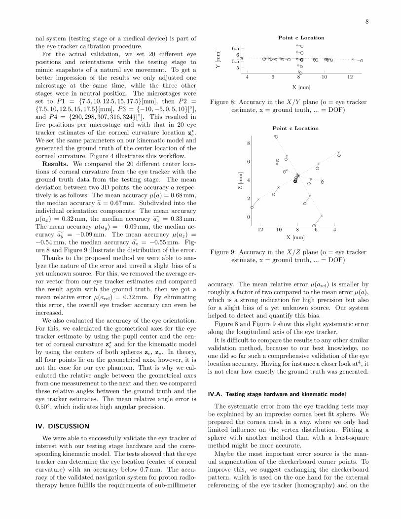
Results. We compared the 20 different center loca-tions of corneal curvature from the eye tracker with theground truth data from the testing stage. The meandeviation between two 3D points, the accuracy a respec-tively is as follows: The mean accuracy µ(a) = 0.68 mm,the median accuracy a = 0.67 mm. Subdivided into theindividual orientation components: The mean accuracyµ(ax) = 0.32 mm, the median accuracy ax = 0.33 mm.The mean accuracy µ(ay) = −0.09 mm, the median ac-curacy ay = −0.09 mm. The mean accuracy µ(az) =−0.54 mm, the median accuracy az = −0.55 mm. Fig-ure 8 and Figure 9 illustrate the distribution of the error.

Thanks to the proposed method we were able to ana-lyze the nature of the error and unveil a slight bias of ayet unknown source. For this, we removed the average er-ror vector from our eye tracker estimates and comparedthe result again with the ground truth, then we got amean relative error µ(arel) = 0.32 mm. By eliminatingthis error, the overall eye tracker accuracy can even beincreased.

We also evaluated the accuracy of the eye orientation.For this, we calculated the geometrical axes for the eyetracker estimate by using the pupil center and the cen-ter of corneal curvature z?c and for the kinematic modelby using the centers of both spheres zc, ze. In theory,all four points lie on the geometrical axis, however, it isnot the case for our eye phantom. That is why we cal-culated the relative angle between the geometrical axesfrom one measurement to the next and then we comparedthese relative angles between the ground truth and theeye tracker estimates. The mean relative angle error is0.50◦, which indicates high angular precision.

IV. DISCUSSION

We were able to successfully validate the eye tracker ofinterest with our testing stage hardware and the corre-sponding kinematic model. The tests showed that the eyetracker can determine the eye location (center of cornealcurvature) with an accuracy below 0.7 mm. The accu-racy of the validated navigation system for proton radio-therapy hence fulfills the requirements of sub-millimeter

4 6 8 10 12

55.5

66.5

X [mm]

Y[m

m]

Point c Location

Figure 8: Accuracy in the X/Y plane (o = eye trackerestimate, x = ground truth, ... = DOF)

4681012

0

2

4

6

8

X [mm]Z

[mm

]

Point c Location

Figure 9: Accuracy in the X/Z plane (o = eye trackerestimate, x = ground truth, ... = DOF)

accuracy. The mean relative error µ(arel) is smaller byroughly a factor of two compared to the mean error µ(a),which is a strong indication for high precision but alsofor a slight bias of a yet unknown source. Our systemhelped to detect and quantify this bias.

Figure 8 and Figure 9 show this slight systematic erroralong the longitudinal axis of the eye tracker.

It is difficult to compare the results to any other similarvalidation method, because to our best knowledge, noone did so far such a comprehensive validation of the eyelocation accuracy. Having for instance a closer look at4, itis not clear how exactly the ground truth was generated.

IV.A. Testing stage hardware and kinematic model

The systematic error from the eye tracking tests maybe explained by an imprecise cornea best fit sphere. Weprepared the cornea mesh in a way, where we only hadlimited influence on the vertex distribution. Fitting asphere with another method than with a least-squaremethod might be more accurate.

Maybe the most important error source is the man-ual segmentation of the checkerboard corner points. Toimprove this, we suggest exchanging the checkerboardpattern, which is used on the one hand for the externalreferencing of the eye tracker (homography) and on the

9

other hand to train and validate the whole testing stagemodel. Hence, the pattern, its segmentation respectively,is central for the validation. A better pattern might bedots in a certain arrangement (similar to the squares inthe checkerboard pattern). This pattern could easily besegmented automatically, by choosing the center of massof the circles or the ellipsoids, respectively, taking thethickness of the ink into account.

IV.B. Eye tracker

Depending on the application different levels of accu-racy are required. Our achieved sub-millimeter accuracyin determining the eye location is sufficient for our med-ical application with especially high demands. If thereshould be higher demands, the detailed validation results,for instance the distribution of the error, might providehelpful information for eye tracker improvement.

V. CONCLUSION

Using an eye tracker to localize the eye in space can po-tentially improve today’s eye interventions. For instance,when treating eye tumors with protons, our non-invasiveeye tracker based solution might some day replace thestate-of-the-art invasive navigation method.

We proposed a quantitative evaluation method withwhich we showed that our eye tracker is able to fulfill therequirements, namely, to determine the location of theeye with sub-millimeter accuracy. Our proposed evalua-tion method does not replace the eye tracker tests withvolunteers that are used nowadays, but it complementsthe validation, enabling new eye tracking applications:eye localization.

We are sure, that in the future more and more appli-cations, especially in ophthalmology, will benefit from aneye localization system.

ACKNOWLEDGMENTS

We would like to thank the members of the Biomate-rials Science Center (BMC) of the University of Baselfor their support with the data acquisition with the µCTsystem. We thank also Otto E. Martin from the SwissInstitute For Artificial Eyes for providing us a hand-crafted eye and for sharing his profound knowledge. Thework is funded by the Swiss National Science Foundation(SNSF).

REFERENCESa)stephan.wyder@unibas.chb)philippe.cattin@unibas.ch1Narcizo Fabricio Batista, Queiroz Jose Eustaquio, Gomes Her-man Martins. Remote Eye Tracking Systems: Technologies andApplications in 2013 26th Conference on Graphics, Patterns andImages Tutorials:15–22IEEE 2013.

2Hansen Dan Witzner, Ji Qiang. In the Eye of the Beholder: ASurvey of Models for Eyes and Gaze Pattern Analysis and Ma-chine Intelligence, IEEE Transactions on. 2010;32:478–500.

3Duchowski Andrew T. Eye tracking methodology - theory andpractice (2. ed.). London: Springer London 2007.

4Via Riccardo, Fassi Aurora, Fattori Giovanni, et al. Opticaleye tracking system for real-time noninvasive tumor localizationin external beam radiotherapy Medical Physics. 2015;42:2194–2202.

5Wyder Stephan, Hennings Fabian, Pezold Simon, Hrbacek Jan,Cattin Philippe C. With Gaze Tracking Toward Noninvasive EyeCancer Treatment Biomedical Engineering, IEEE Transactionson. 2016;63:1914–1924.

6Wyder Stephan, Cattin Philippe C. Stereo Eye Tracking with aSingle Camera for Ocular Tumor Therapy in Proceedings of theOphthalmic Medical Image Analysis International Workshop:81–88 2016.

7Swirski Lech, Dodgson Neil. Rendering synthetic ground truthimages for eye tracker evaluation in Proceedings of the 2014 Sym-posium on Eye-Tracking Research & Applications(New York,New York, USA):219–222ACM 2014.

8Guestrin Elias Daniel, Eizenman Moshe. General theory ofremote gaze estimation using the pupil center and cornealreflections Biomedical Engineering, IEEE Transactions on.2006;53:1124–1133.

9Schindelin Johannes, Arganda-Carreras Ignacio, Frise Erwin, etal. Fiji: an open-source platform for biological-image analysisNature Methods. 2012;9:676–682.

10Leon Steven J. Linear algebra with applications Macmillan NewYork 1980.

11Besl P J, McKay H D. A method for registration of 3-D shapesIEEE Transactions on Pattern Analysis and Machine Intelli-gence. 1992;14:239–256.

12Zhang Zhengyou. A flexible new technique for camera calibrationPattern Analysis and Machine Intelligence, IEEE Transactionson. 2000;22:1330–1334.