exports and volatility...
TRANSCRIPT

Exports and Volatility Spillovers
Sourafel Girma:Alejandro Riano;
July 29, 2016
Preliminary and Incomplete.Please do not cite without permission.
Abstract
Firms that participate in international markets, be it through exporting, importing or setting upforeign subsidiaries tend to be more volatile than their domestic counterparts. In this paper weask whether the higher volatility of stock returns of exporting firms spills over to firms that onlysell domestically. We utilize weekly data for the universe of manufacturing firms listed in theTokyo Stock Exchange over the period 2000-2015 to investigate this question. We find evidenceof substantial spillovers of volatility occurring among exporters and non-exporters. Our resultsalso show that — consistent with a workhorse model of trade with stochastic volatility — thereis an important asymmetry in volatility spillovers. The spillovers from exporters to domesticfirms are on average twice as large as the spillovers in the opposite direction.
Keywords: Volatility; Spillovers; Stock Returns; Exports; Japan.JEL classification: F36, F14, G15.
We are thankful to Ana Galvao, Marek Raczko, Costas Theodoridis and participants at the CFCM Workshopon Volatility, Uncertainty and Monetary Policy at the University of Nottingham for their helpful comments. Allremaining errors are our own.
:University of Nottingham, GEP and CFCM. [email protected];University of Nottingham, GEP, CFCM and CESifo. [email protected]

1 Introduction
As financial markets have become progressively more interdependent, the possibility that shocks
originating in far-away places spread rapidly across countries wreaking havoc in local asset markets
has become a permanent source of worry for policymakers and investors. There is indeed an
extensive body of literature devoted to identify the extent to which economic crisis are transmitted
internationally across real and financial linkages.1 At the same time, a small but growing body
of work with a more microeconomic perspective has found that internationally engaged firms are
more volatile across a range of performance measures (e.g. sales, employment, stock returns) than
firms that only sell domestically.2
In this paper we seek to bring together these two strands of the literature, and ask whether
the higher volatility that characterizes exporting firms is transmitted to domestic firms through
their inter-dependence in domestic product and factor markets. Thus, our aim is to shed light on
the domestic diffusion of international shocks. As Ehrmann et al. (2011) note, the transmission
channels through which shocks dissipate across financial markets are still not well understood.
To illustrate the mechanism we study, take the standard Melitz (2003) model of international
trade with heterogenous firms. In this model, an increase in the profitability of exporting (e.g.
due to a bilateral tariff reduction) increases the demand for labor for exporters, pushing up wages
and thereby lowering the profitability of domestic firms. Similarly, via the trade-balance market
clearing condition, the expansion of domestic exports is compensated by an increase in imports,
which intensifies the level of competition, hurting once again firms that only operate domestically.
We illustrate the existence of volatility spillovers in a standard dynamic general equilibrium
model of trade with heterogenous firms along the lines of Alessandria and Choi (2007) and Fillat and
Garetto (2015), which incorporates firm-destination-specific stochastic volatility in demand shocks,
following Arellano et al. (2011) and Fernandez-Villaverde et al. (2015). In the model exporting
entails substantial sunk entry costs (Roberts and Tybout, 1997), which result in exporting firms
being more volatile than their domestic counterparts, as shown by Riano (2011) and Fillat and
Garetto (2015). Our main contribution relative to the previous literature, is to show that in
1See e.g. Forbes and Rigobon (2002), Forbes (2004), Brooks and Del Negro (2004), Corsetti et al. (2005), Ehrmannet al. (2011), and the survey by Pericoli and Sbracia (2003), among many others.
2See Buch et al. (2009), Riano (2011), Vannoorenberghe (2012), Girma et al. (2015) and Kurz and Senses (2016).
1

general equilibrium, the higher volatility of exporters is in turn transmitted to domestic producers
in general equilibrium.
We utilize high-frequency (weekly) data on stock returns for the universe of manufacturing
firms listed in the Tokyo Stock Exchange. In previous work, Girma et al. (2015) have shown that
both exporters and multinational Japanese listed firms are more volatile than domestic firms in
terms of their stock returns. Moreover, and in line with a large body of literature in finance,
Girma et al. (2015) find strong evidence of time-variation in the volatility of firm returns. We
use the methodology developed by Diebold and Yilmaz (2009) and Diebold and Yilmaz (2012)
to measure volatility spillovers from exporters towards domestic firms. This involves estimating a
bivariate VAR model of the conditional volatility (which has been estimated in a previous stage
using a GARCH model) of returns of a value-weighted portfolio of firms constructed based on their
export status and carrying out a generalized forecast error variance decomposition (Pesaran and
Shin, 1998). We also estimate a larger VAR system including the volatility of the S&P-500 index,
as a measure of global volatility, as well as the conditional volatilities of the nominal Yen/Dollar
exchange rate and the volatility of listed banks.
Both our benchmark and augmented specifications show that volatility spillovers are substantial
at different forecast horizons. To be precise, a shock to the volatility of returns of the portfolio of
exporters in our sample accounts for between 40 to 53% of the error variance in forecasting the
volatility of returns for the portfolio of domestic firms over a month. We also find evidence of
volatility spillovers from domestic firms to exporters, although these tend to be about half of the
size of spillovers originating from exporters. Volatility spillovers from exporters dissipate over time,
but still account for 20% of the forecast error of the volatility of non-exporters after 6 months.
Estimating our model using 6 month rolling-window samples shows that the magnitude of the
spillovers has remained quite stable over time and does not appear to vary along the business cycle.
Our results are closely complementary to those of Forbes and Chinn (2004), who find that
bilateral trade are the most important determinant of cross-country linkages in stock markets. We
show that intra-industry forces such as product and factor market competition result in domestic
firms, i.e. those that only sell their output in the local market, becoming more volatile through
their interaction with globally-engaged firms in the same industry. Our results are also relevant
to inform the debate on the potential gains of international portfolio diversification (Heston and
2

Rouwenhorst, 1994; Griffin and Andrew Karolyi, 1998; Brooks and Del Negro, 2004; Bekaert et al.,
2009). If operating in international markets is associated with a higher volatility of stock returns –
as Girma et al. (2015) find for Japanese manufacturing firms – the extent to which an investor can
reduce the variance of a portfolio that combining stocks of domestic firms and exporters operating
in the same industry will be lowered if the latters volatility spills over onto the former.
The rest of the paper is organized as follows. Section 2 sketches a model that illustrates how
product market competition results in volatility spilling over from exporters towards domestic firms,
the mechanism that we analyze in the paper. Section 3 describes our data and empirical specifica-
tions. Section 4 presents our main results and robustness checks. Finally, Section 5 concludes.
2 A Simple Model of Exporting and Volatility Spillovers
The world consists of two symmetric countries, home and foreign. We denote foreign variables by
an asterisk. Each country is populated by a mass L of atomistic households, who supply one unit
of labor inelastically at the prevailing wage.
Preferences. The representative consumer maximizes the expected discounted sum of utility,
U E0
¸8
t0βtupCtq
, (1)
where Ct denotes final consumption, and β P p0, 1q is the subjective discount factor. We assume
that instantaneous utility takes the form, upCq C1γp1 γq, where γ ¡ 0 is the coefficient of
relative risk aversion.
Following Alessandria and Choi (2014), we assume there is a one-period nominal bond denom-
inated in units of the home final good — thus, the bond pays one unit of home’s final good in
the next period. Let Bt denote the bond holdings of home consumers and Qt its nominal price.
Choosing home’s final good as the numeraire, Pt 1 implies that P t 1 and Bt B
t 0 (i.e.
balanced trade), given our assumption of symmetric countries. Every period, home consumers face
the following budget constraint (foreign consumers face an analogous constraint):
Ct QtBt WtLBt1 Πt, (2)
3
where Wt is the wage prevailing at home and Πt denotes the dividend payments from home firms.
Final Good Production. The consumption good C, which is non-tradable, is produced under
perfect competition using a continuum of differentiated domestic and imported intermediate goods:
Yt
» 1
0pqdtpωqq
ε1ε dω
»ωPΩ
x
pqxtpωqqε1ε dω
εε1
, (3)
where qdtpωq and qxtpωq denote domestic and imported intermediate inputs respectively and ε ¡ 1
is the elasticity of substitution between intermediate inputs. Since trade in intermediate inputs is
costly, home’s final-good production incorporates only a subset Ωx of intermediate inputs that are
produced and exported from foreign, while utilizing the complete range of locally-produced inputs.
Intermediate input demand is given by:
qdtpωq YtPε1t rpdtpωqs
ε, (4)
qxtpωq YtPε1t rpxtpωqs
ε, (5)
where pdtpωq and pxtpωq denote respectively the price of domestic and intermediate inputs, Yt is
the total value of home’s final goods, and Pt is the ideal price index, defined as:
Pt
» 1
0ppdtpωqq
1ε dω
»ωPΩ
x
ppxtpωqq1ε dω
11ε
. (6)
Intermediate Good Production. Intermediate good producers are monopolistically-competitive,
producing their output using a 1-1 technology, with labor being the only input. These firms can
sell their output domestically (d) or export it to the rest of the world (x). We assume that all
intermediate producers have the same marginal cost of production, but are heterogeneous in terms
of their idiosyncratic destination-specific demand shocks tzjtpωqu, j P td, xu. We assume that
firm-destination specific shocks exhibit stochastic volatility, following Fernandez-Villaverde et al.
(2015):
log zjt λj log zj,t1 σjtξjt, ξjt N p0, 1q (7)
log σjt p1 ρjq log σj ρj log σj,t1 ηujt, ujt N p0, 1q. (8)
4

Export is costly. Firms need to incur a fixed sunk cost Sx when they start to export, but only need
to pay Fx, with Fx Sx, if they have exported in the previous period (Baldwin and Krugman,
1989; Roberts and Tybout, 1997; Alessandria and Choi, 2007; Fillat and Garetto, 2015). Moreover,
export sales are subject to an iceberg transport cost τ ¡ 1. Let yt P t0, 1u denote a firm’s export
status in period t, with yt 1 if a firm exports in period t and 0 otherwise. Home exporters faces
a downward-sloping demand abroad:
rxtpωq Axzxtpωqpxtpωq1ε, Ax ¡ 0. (9)
The only difference with their domestic demand (4) is that the pricing decision of Home’s interme-
diate good producers do not influence aggregate expenditure nor the price index in the rest of the
world (see Demidova and Rodrıguez-Clare, 2009, 2013).
Firms’ problem. An intermediate good producer’s state vector s consists of its previous-year
export status, y1, as well as domestic and export demand shocks and their respective variances:
s pzd, σd, zx, σxq. Intermediate good producers’ problem can be partitioned into a static and a
dynamic component. In any given period, a firm charges a constant mark-up above its marginal cost
domestically, i.e. pdtpy1, sq εε1wt, while charging the same price augmented by the transport
cost τ if it exports, pxtpy1, sq τpdtpy1, sq.
At each point in time, a firm needs to choose whether to export or not, i.e. y P t0, 1u based
on its previous-year export status y1 and the realization of demand shocks and their variances.
Thus, the dynamic programming problem of an intermediate-good producer can be expressed in
recursive form:
vpy1, sq maxyPt0,1u
"πpy1, y, sq M
»s1Pps1|sqvpy, s1qds1
*, (10)
where v is the market value of a firm, M is the stochastic discount factor, P is a transition matrix
for firm-destination-specific demand shifters and their volatilities and a firm’s dividends are given
by:
πpy1, y, sq κw1ε Adzd y
τ1εAxzx w py1Fx p1 y1qSxq
(. (11)
5

and κ pε 1qε1εε. The solution to problem (10) is an export policy rule Ypy1, sq.
General Equilibrium. A recursive stationary equilibrium is defined by an export policy rule
Ypy1, sq and a vector of prices tw, P u such that:
(i) The labor market clears at Home, and,
(ii) The current account is balanced.
Stock market returns in this model are defined as follows:
Rpy, sq πpy1, sq
vpy1, sq.
Solution and Parametrization. We solve the model using a value function iteration algorithm.
We parametrize the fixed and sunk costs in the model in order to match the share of exporters
observed in our sample (23%). We set the same persistence in the level of shocks and their variance
across destination markets, namely, we set λj 0.7 and ρj 0.1; the variance of the variance, ηj
is set to 0.01.
In order to highlight the main predictions of the model, we simulate 10,000 firms and compute
the return of a value-weighted market portfolio of firms based on their export status. As has been
pointed out before by Riano (2011) and Fillat and Garetto (2015), the existence of sunk costs asso-
ciated with a firm’s decision to start to export increase the volatility of a firm’s performance. The
hysteresis induced by the sunk costs makes managers reluctant to stop exporting when profitability
falls, because the option value of waiting for it to improve outweighes the cost of re-incurring the
entry costs again. This effect is evident in Figure 1, which displays the distribution of market-
value-weighted stock returns for exporters and non-exporters. Even though the stochastic process
governing domestic and export demand shifters have the same parameters, the volatility of stock
returns is substantially higher for exporters than for firms that only sell domestically.
We next use the methodology developed by Diebold and Yilmaz (2009) and Diebold and Yilmaz
(2012) (which is explained in more detail in the next section) in the simulated data generated by
the model. We find that volatility spillovers from exporters account for 15-20% of the forecast error
variance of the conditional volatility of non-exporters. Conversely, domestic firms exert a negligible
6

effect on the volatility of returns of exporters. In the next two sections we show that the existence
of volatility spillovers from exporters to domestic firms and the larger magnitude of these spillovers
when originating from exporters are also found in our dataset of Japanese manufacturing firms.
Figure 1: Stationary Distribution of Stock Returns by Export Status
−0.2 −0.1 0 0.1 0.2 0.3 0.4 0.50
5
10
15
Market−value−weighted returns
Den
sity
Non−ExportersExporters
3 Data and Empirical Specification
Data
We use weekly data for the universe of manufacturing firms listed in the Tokyo Stock Exchange
between 2000:w1 until 2015:w52. We construct two market-value-weighted portfolios of firms based
on their export status j P td, xu. We estimate an ARMA model for the conditional mean of excess
stock returns and a GARCH(1,1) model for the conditional volatility of each portfolio, hjt . Predicted
conditional volatilities are annualized as 100
b52 hjt
.
Table 1 presents summary statistics for each of our constructed portfolios. The main character-
istics of the two groups of firms conform to the stylized facts established in the existing literature.
Namely, exporters are larger (in terms of their market capitalization), exhibit higher returns and
are more volatile than their domestic counterparts (Bernard et al., 2007; Fillat and Garetto, 2015;
7

Table 1: Descriptive Statistics
Non-exporters Exporters
Mean Std Dev Mean Std Dev
Stock return -0.013 2.890 0.013 2.577Log volatility 2.785 0.887 2.859 0.725Log market value 11.612 3.625 13.363 3.600Log spillover term exporters 2.347 0.649 2.353 0.647Log spillover term non-exporters 2.165 0.666 2.194 0.670
Number of firms 1,858 551Observations 1,247,345 448,512
Girma et al., 2015).
Figure 2 displays the evolution of the conditional volatility of stock returns for our export-status-
based portfolios throughout our period of study. Volatility exhibits a high degree of time-series
variation and large spikes during recessions (Schwert, 1989; Bloom, 2014). Although the volatility
of returns for both types of firms show a substantial degree of comovement, it is also apparent that
the volatility of exporters has been systematically higher than that of non-exporters since 2005.
8

Figure 2: Conditional Volatility by Export Status
ExportersNon-exporters
010
2030
40C
ondi
tiona
l vol
atili
ty o
f ret
urns
2000w1 2005w1 2010w1 2015w1Time
The figure plots the conditional volatility of returns of the portfolios composed by domestic firmsand exporters. Conditional volatility is estimated using a GARCH(1,1) model using weekly datafor the period 2000w1-2015w52. Shaded areas denote recession periods in Japan identified by theOECD (series JPNRECM from St Louis Fed FRED database). Recession periods in our sample are:2001:m2-2002:m1; 2004:m3-2004:m12; 2008:m2-2009:m4; 2010:m8-2012:m9 and 2014:m1-2014:m8.
Empirical Specification
Benchmark Specification. In order to identify the existence of volatility spillovers occurring
between exporters and non-exporters, we make use of the methodology proposed by Diebold and
Yilmaz (2009) and Diebold and Yilmaz (2012). In our benchmark specification, estimate a reduced-
form bi-variate VAR model for the conditional volatility of stock returns for our export-based
portfolios, yt phxt , hdt q1:
yt ¸p
i1Φiyti εt, ε p0,Σq, (12)
where Φi are 2 2 matrices of coefficients to be estimated and εt is an error term with covariance
matrix Σ.
Volatility spillovers are recovered by conducting a τ -step ahead generalized forecast error vari-
ance decomposition (FEVD) based on the estimates of model (12), i.e. ytτ Etrytτ s. Thus, our
measure of spillovers is the fraction of the τ -step-ahead forecast error variance for the conditional
9

volatility of portfolio j that is explained by shocks to the conditional volatility of portfolio k j. We
use a generalized FEVD proposed by Pesaran and Shin (1998), which, unlike a Cholesky-identified
variance decomposition, is invariant to variable ordering:
θgjkpτq σ1jj
°τl0pe
1jAlΣekq
2°τl0 e
1jAlΣA
1lej, j, k P td, xu, (13)
where Al are the coefficients associated with the MA representation of the VAR model (12), and
ej is a unit vector that takes the value 1 in its j-th position and 0 elsewhere.
Since the generalized FEVD does not orthogonalize shocks but rather takes into account their
correlation, it follows that°k θ
gjkpτq does not sum up to 1 as in the standard Cholesky-identified
FEVD. Thus, following Diebold and Yilmaz (2012), we define the pairwise spillovers from portfolio
j to portfolio k at horizon τ as:
Sjkpτq θgjkpτq°
`Ptd,xu θgj`pτq
P r0, 1s, τ 0, 1, . . . (14)
We also utilize an unconditional measure of volatility to estimate spillovers. In this case, volatility
is estimated using the range-based method proposed by Alizadeh et al. (2002) from the underlying
daily high/low/open/close stock data to obtain a measure of weekly volatility of returns, which is
annualized in the same way described above.
Augmented Model. An important concern in our benchmark specification is that our measure of
volatility spillovers could be capturing a common global factor affecting the volatility of exporters
and non-exporters in Japan (see e.g. Kose et al., 2003). To address this issue, we augment our
simple bi-variate VAR model to include a host of factors suggested by the literature, which could
drive the conditional volatility of Japanese firms.
The new variables incorporated into our VAR model are (i) the conditional volatility of returns
for the S&P-500 index, (ii) the conditional volatility of the Japanese Yen/US Dollar exchange rate
and (iii) the conditional volatility of listed Japanese banks. The first variable controls for world-
wide changes in volatility; The volatility of the exchange rate has been shown to be an important
determinant of returns volatility (Girma et al., 2015) for listed Japanese firms, and lastly, the
10

volatility of the banking sector seeks to control for the higher intensity of use of financial services
by exporters relative to domestic firms, as documented by Amiti and Weinstein (2011), Manova
(2013) and Girma et al. (2015).
Microeconometric Specification. In our last specification, we rely on individual firm-level data,
to estimate the following linear dynamic panel for both exporters and domestic firms separately:
ln hit β0 ln hit1 γx ln Spilloverxt1 γd ln Spilloverdt1 β1 ln Market Valueit1 β2Tt fi uit,
(15)
where hit denotes the predicted conditional volatility of stock returns for firm i in week t estimated
using a GARCH(1,1) model for each individual firm, Spilloverxt1 denotes the conditional volatility
of the return of the value-weighted portfolio of exporters excluding firm i (lagged one week), and
Spilloverdt1 is the analogous measure for a portfolio of domestic firms; Market Valueit1 is firm i’s
market capitalization, Tt is a linear trend, fi denote firm-specific fixed effects and uit is the error
term. Standard errors are clustered at the firm level.
4 Results
Benchmark Model. Table 2 presents the results using our benchmark bi-variate specification.
The main message is clear — spillovers originating from exporting firms explain a substantial share
of the forecast error variance of the conditional volatility of domestic firms. Conversely — and
just as predicted by the model presented in Section 2 — the volatility of domestic firms exerts a
smaller role in the volatility of exporters; the magnitude of the spillover term from exporters to
domestic firms is approximately twice as large across different forecast horizon. In columns (3) and
(4), we augment our benchmark model with linear, quadratic and cubic trends that can flexibly
account for common factors driving the conditional volatility of our two portfolios. Reassuringly,
our results remain unchanged; we still find a remarkable asymmetry in the magnitude of volatility
spillovers occurring among groups of firms based on their export participation status. Columns (5)
and (6) replicate our benchmark exercise, but using the unconditional volatility of returns. Once
again, the results remain robust to this change in specification.
11
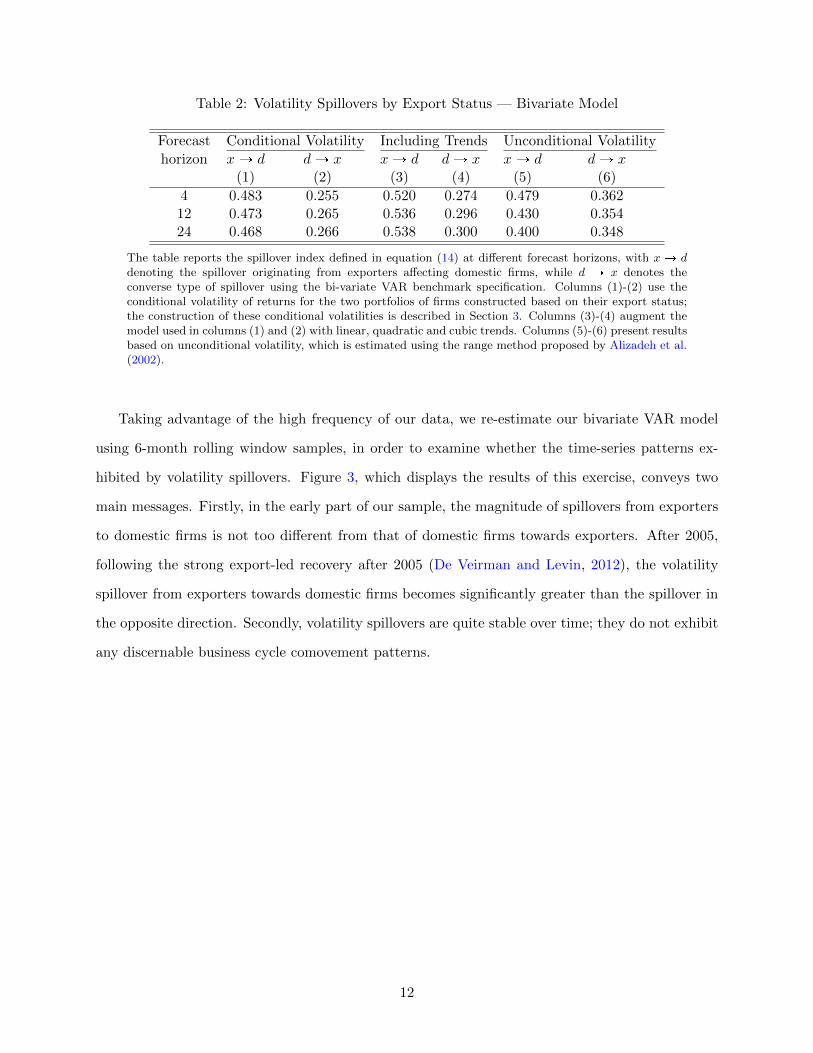
Table 2: Volatility Spillovers by Export Status — Bivariate Model
Forecast Conditional Volatility Including Trends Unconditional Volatility
horizon xÑ d dÑ x xÑ d dÑ x xÑ d dÑ x(1) (2) (3) (4) (5) (6)
4 0.483 0.255 0.520 0.274 0.479 0.36212 0.473 0.265 0.536 0.296 0.430 0.35424 0.468 0.266 0.538 0.300 0.400 0.348
The table reports the spillover index defined in equation (14) at different forecast horizons, with x Ñ ddenoting the spillover originating from exporters affecting domestic firms, while d Ñ x denotes theconverse type of spillover using the bi-variate VAR benchmark specification. Columns (1)-(2) use theconditional volatility of returns for the two portfolios of firms constructed based on their export status;the construction of these conditional volatilities is described in Section 3. Columns (3)-(4) augment themodel used in columns (1) and (2) with linear, quadratic and cubic trends. Columns (5)-(6) present resultsbased on unconditional volatility, which is estimated using the range method proposed by Alizadeh et al.(2002).
Taking advantage of the high frequency of our data, we re-estimate our bivariate VAR model
using 6-month rolling window samples, in order to examine whether the time-series patterns ex-
hibited by volatility spillovers. Figure 3, which displays the results of this exercise, conveys two
main messages. Firstly, in the early part of our sample, the magnitude of spillovers from exporters
to domestic firms is not too different from that of domestic firms towards exporters. After 2005,
following the strong export-led recovery after 2005 (De Veirman and Levin, 2012), the volatility
spillover from exporters towards domestic firms becomes significantly greater than the spillover in
the opposite direction. Secondly, volatility spillovers are quite stable over time; they do not exhibit
any discernable business cycle comovement patterns.
12

Figure 3: Volatility Spillovers over Time
0.2
.4.6
.81
Spi
llove
r ind
ex
2000h1 2005h1 2010h1 2015h1Time
From Exporters to Non-ExportersFrom Non-Exporters to Exporters
The figure plots both the spillover index from exporters towards domestic firms and from domestic firms to exportersestimated using the bivariate VAR model (12) using 6-month rolling windows. Shaded areas denote recession periodsin Japan identified by the OECD (series JPNRECM from St Louis Fed FRED database). Recession periods in oursample are: 2001:m2-2002:m1; 2004:m3-2004:m12; 2008:m2-2009:m4; 2010:m8-2012:m9 and 2014:m1-2014:m8.
Augmented Model
Table 3 presents the estimated volatility spillovers based on our augmented VAR model using 4
and 24-weeks forecast horizons. The results show that global volatility, proxied by the conditional
volatility of returns of the S&P-500 index has a moderate effect on the volatility of our export-based
portfolios, exerting a larger effect on exporters than on domestic firms. Shocks to exchange rate
volatility, on the other hand, appear to have a negligible contribution to the volatility of our two
groups of firms; lastly, the volatility of listed banks has an effect which is twice as large as that of
global shocks, and this effect is also slightly more important for exporters than for domestic firms,
in line with the findings by Amiti and Weinstein (2011) for Japanese firms.
The magnitude of volatility spillovers from exporters to domestic firms remains substantial in
the extended model. Shocks to the conditional volatility of exporters contribute to explain 40%
of the forecast error for the volatility of returns of domestic firms falls relative to our bivariate
13

Table 3: Volatility Spillovers by Export Status — Augmented Model
4-week ahead forecast
From:S&P 500 U$ Banks x d
S&P 500 0.892 0.009 0.075 0.010 0.014U$ 0.308 0.211 0.204 0.234 0.044
To: Banks 0.033 0.001 0.596 0.228 0.142x 0.061 0.002 0.142 0.621 0.174d 0.057 0.005 0.131 0.400 0.408
24-week ahead forecast
From:S&P 500 U$ Banks x d
S&P 500 0.701 0.002 0.256 0.003 0.037U$ 0.367 0.092 0.458 0.067 0.016
To: Banks 0.073 0.000 0.741 0.112 0.073x 0.118 0.001 0.378 0.391 0.112d 0.114 0.002 0.368 0.206 0.309
The table reports the spillover index defined in equation (14) at 4 and 24-weekforecast horizons. The pi, jqth entry in the table denotes the fraction of the forecastvariance of variable j (column) explained by shocks in the variable i (row). Therows of the table sum up to 1, given the definition of the spillover index. Theadditional variables included in the VAR system besides the conditional volatilityof returns for exporters and non-exporters are the conditional volatility of returnsfor the S&P-500 index estimated using a GARCH(1,1) model, the conditionalvolatility of the Japanese Yen/US Dollar nominal exchange rate estimated using aGARCH(1,1) and the conditional volatility of returns for banks listed in the TokyoStock Exchange.
14

benchmark. These spillovers are again, about twice as large as those originating in domestic firms.
The main difference with respect to our benchmark specification is that the size of spillovers de-
cline more rapidly with the forecast horizon in the extended model. Still, volatility spillovers from
exporters account for one-fifth of the variance in the conditional conditional volatility of returns of
domestic firms after 6 months.
Exports and Volatility Spillovers: A Microeconometric View. The evidence presented
regarding the existence of the volatility of exporters spilling over to domestic producers relies on
a macro-econometric approach that on the one hand allows for bidirectional spillovers to exist.
However, by aggregating firms into export-based portfolios, this approach might miss important
micro-level heterogeneity. Thus, Table 4 presents the results of using a microeconometric approach
to explore the existence of volatility spillovers.
The conditional volatility of returns for a given firm i depends on its own lagged volatility —,
since this variable is highly persistent — and on the firm’s size. Crucially, however, it also depends
on the conditional volatility of the portfolio of exporters and domestic firms that excludes firm i.
Controlling for firm fixed effects and linear trends, we find that the spillover terms have a strong and
positive effect in explaining firm-level volatility. Our results show that the volatility of exporters
has a stronger effect on firm-level volatility than the volatility of domestic firms. Moreover, the
volatility spillover for exporters has a bigger effect in the volatility of domestic firms than the
converse. All in all, spillovers originating from exporters are approximately 1.5 times larger than
spillovers from domestic firms to exporters — a similar magnitude to the one reported above.
5 Conclusions
TBA
15

Table 4: Exports and Volatility Spillovers: A Microeconometric View
Non-exporters Exporters(1) (2)
Lagged volatility 0.209*** 0.182***(0.002) (0.003)
Lagged spillover from exporters 0.071*** 0.095***(0.002) (0.003)
Lagged spillover from non-exporters 0.027*** 0.049***(0.002) (0.003)
Market value -0.003*** -0.008***(0.001) (0.001)
Time trend -0.0003*** -0.0001***(0.000) (0.000)
Firm fixed effects y yObservations 1,200,833 445,860
* p 0.10, ** p 0.05, *** p 0.01. Standard errors clustered at the firm level.
References
Alessandria, G. and H. Choi (2007): “Do Sunk Costs of Exporting Matter for Net ExportDynamics?” Quarterly Journal of Economics, 122, 289–336.
——— (2014): “Establishment heterogeneity, exporter dynamics, and the effects of trade liberal-ization,” Journal of International Economics, 94, 207–223.
Alizadeh, S., M. W. Brandt, and F. X. Diebold (2002): “Range-Based Estimation ofStochastic Volatility Models,” Journal of Finance, 57, 1047–1091.
Amiti, M. and D. E. Weinstein (2011): “Exports and Financial Shocks,” The Quarterly Journalof Economics, 126, 1841–1877.
Arellano, C., Y. Bai, and P. Kehoe (2011): “Financial Markets and Fluctuations in Uncer-tainty,” Meeting Papers 896, Society for Economic Dynamics.
Baldwin, R. and P. R. Krugman (1989): “Persistent Trade Effects of Large Exchange RateShocks,” Quarterly Journal of Economics, 104, 635–654.
Bekaert, G., R. J. Hodrick, and X. Zhang (2009): “International Stock Return Comove-ments,” Journal of Finance, 64, 2591–2626.
Bernard, A. B., J. B. Jensen, S. J. Redding, and P. K. Schott (2007): “Firms in Inter-national Trade,” Journal of Economic Perspectives, 21, 105–130.
Bloom, N. (2014): “Fluctuations in Uncertainty,” Journal of Economic Perspectives, 28, 153–76.
Brooks, R. and M. Del Negro (2004): “The rise in comovement across national stock markets:market integration or IT bubble?” Journal of Empirical Finance, 11, 659–680.
16

Buch, C. M., J. Dopke, and H. Strotmann (2009): “Does Export Openness Increase Firm-level Output Volatility?” The World Economy, 32, 531–551.
Corsetti, G., M. Pericoli, and M. Sbracia (2005): “’Some contagion, some interdependence’:More pitfalls in tests of financial contagion,” Journal of International Money and Finance, 24,1177–1199.
De Veirman, E. and A. T. Levin (2012): “When did Firms Become More Different? Time-varying Firm-specific Volatility in Japan,” Journal of the Japanese and International Economies,26, 578–601.
Demidova, S. and A. Rodrıguez-Clare (2009): “Trade Policy Under Firm-level Heterogeneityin a Small Economy,” Journal of International Economics, 78, 100–112.
——— (2013): “The simple analytics of the Melitz model in a small economy,” Journal of Inter-national Economics, 90, 266–272.
Diebold, F. X. and K. Yilmaz (2009): “Measuring Financial Asset Return and VolatilitySpillovers, with Application to Global Equity Markets,” Economic Journal, 119, 158–171.
——— (2012): “Better to give than to receive: Predictive directional measurement of volatilityspillovers,” International Journal of Forecasting, 28, 57–66.
Ehrmann, M., M. Fratzscher, and R. Rigobon (2011): “Stocks, bonds, money markets andexchange rates: measuring international financial transmission,” Journal of Applied Economet-rics, 26, 948–974.
Fernandez-Villaverde, J., P. Guerron-Quintana, and J. F. Rubio-Ramırez (2015): “Es-timating dynamic equilibrium models with stochastic volatility,” Journal of Econometrics, 185,216–229.
Fillat, J. L. and S. Garetto (2015): “Risk, Returns, and Multinational Production,” TheQuarterly Journal of Economics, 130, 2027–2073.
Forbes, K. J. (2004): “The Asian Flu and Russian Virus: The International Transmission ofCrises in Firm-level Data,” Journal of International Economics, 63, 59–92.
Forbes, K. J. and M. D. Chinn (2004): “A Decomposition of Global Linkages in FinancialMarkets Over Time,” The Review of Economics and Statistics, 86, 705–722.
Forbes, K. J. and R. Rigobon (2002): “No Contagion, Only Interdependence: Measuring StockMarket Comovements,” Journal of Finance, 57, 2223–2261.
Girma, S., S. P. Lancheros, and A. Riano (2015): “Global Engagement and Returns Volatil-ity,” CFCM Working Paper 2015/12.
Griffin, J. M. and G. Andrew Karolyi (1998): “Another look at the role of the industrialstructure of markets for international diversification strategies,” Journal of Financial Economics,50, 351–373.
Heston, S. L. and K. G. Rouwenhorst (1994): “Does industrial structure explain the benefitsof international diversification?” Journal of Financial Economics, 36, 3–27.
17

Kose, M. A., C. Otrok, and C. H. Whiteman (2003): “International Business Cycles: World,Region, and Country-Specific Factors,” American Economic Review, 93, 1216–1239.
Kurz, C. J. and M. Z. Senses (2016): “Importing, exporting, and firm-level employment volatil-ity,” Journal of International Economics, 98, 160 – 175.
Manova, K. (2013): “Credit Constraints, Heterogeneous Firms, and International Trade,” Reviewof Economic Studies, 80, 711–744.
Melitz, M. J. (2003): “The Impact of Trade on Intra-Industry Reallocations and AggregateProductivity,” Econometrica, 71, 1695–1725.
Pericoli, M. and M. Sbracia (2003): “A Primer on Financial Contagion,” Journal of EconomicSurveys, 17, 571–608.
Pesaran, H. H. and Y. Shin (1998): “Generalized impulse response analysis in linear multivariatemodels,” Economics Letters, 58, 17–29.
Riano, A. (2011): “Exports, Investment and Firm-level Sales Volatility,” Review of World Eco-nomics (Weltwirtschaftliches Archiv), 147, 643–663.
Roberts, M. J. and J. R. Tybout (1997): “The Decision to Export in Colombia: An EmpiricalModel of Entry with Sunk Costs,” American Economic Review, 87, 545–564.
Schwert, G. W. (1989): “Why Does Stock Market Volatility Change over Time?” Journal ofFinance, 44, 1115–53.
Vannoorenberghe, G. (2012): “Firm-level Volatility and Exports,” Journal of InternationalEconomics, 86, 57–67.
18