EXPLORING WHITE-COLLAR CRIME AND THE AMERICAN DREAM

By

ANDREA SCHOEPFER

A THESIS PRESENTED TO THE GRADUATE SCHOOL OF THE UNIVERSITY OF FLORIDA IN PARTIAL FULFILLMENT OF THE REQUIREMENTS FOR THE

DEGREE OF MASTER OF ARTS

UNIVERSITY OF FLORIDA

2004

Copyright 2004

by

Andrea Schoepfer

TABLE OF CONTENTS Page

LIST OF TABLES....…………………….………………………………………….…….v ABSTRACT ………………………………………………………………………….....vii CHAPTER 1 INTRODUCTION …………………………………………………….………….1 2 LITERATURE REVIEW…………………………………………………………7 Institutional Anomie Theory (IAT)….……………………………………………7 Institutional Anomie Theory Empirical Studies……........………………………10 3 DATA AND METHODS……………………………………………………..…17 Data…………………..…………………………………………………………..17

Dependent Variables…………..…………………………………………18 Independent Variables.....……….……………………………………….19

Hypotheses……………………………………………..………………………...21 Analytic Plan…………………..…………………………………………………21 4 RESULTS...………………………..………………….…………………………23 Total White-Collar Crime Rates………………….…………………………….. 23 Fraud Rates……………………………………..………………………………..26 Forgery/Counterfeiting Rates…………………..………………………………..28 Embezzlement Rates………………………….…………………………………30 Alternate Findings……………………………………….………………………32

5 DISCUSSION AND CONCLUSION……………………..…………………….39 Discussion………………………………………………..………………………39 Limitations and Future Research………………………..……………………….41

iii

APPENDIX A POISSON ESTIMATES FOR THE ALTERNATE FAMILY MEASURE…….44

B POISSON ESTIMATES FOR THE ALTERNATE ECONOMY MEASURE…48

C POISSON ESTIMATES FOR THE ALTERNATE EDUCATION

MEASURE………………………………………………………………52 REFERENCE LIST…….……………………….…………….…………………………56 BIOGRAPHICAL SKETCH…………………………………………………………… 59

iv

LIST OF TABLES Table page 1 Descriptive Statistics for 1990 – 1991 Variables………….………………..……18 2 Descriptive Statistics for 2000 Variables…………………….…..………………18 3 Institutional Anomie Theory Expected Effects..…………………………………22 4 Poisson Estimates for Total White-Collar Crime Rates 1991….………………..24 5 Poisson Estimates for Total White-Collar Crime Rates 2000 …….…………….26

6 Poisson Estimates for Fraud Rates 1991 ………..……………..………………. 27 7 Poisson Estimates for Fraud Rates 2000 ……..……………..…………………. 28 8 Poisson Estimates for Forgery/Counterfeiting Rates 1991……………..……… 29 9 Poisson Estimates for Forgery/Counterfeiting Rates 2000…..………………… 30 10 Poisson Estimates for Embezzlement Rates 1991….………….………………. 31 11 Poisson Estimates for Embezzlement Rates 2000...…...…………..……..……..32 A-1 Poisson Estimates for Total White-Collar Crime Rate 1991…………..………..44 A-2 Poisson Estimates for Fraud Rates 1991………………………………………..44 A-3 Poisson Estimates for Forgery/Counterfeiting Rates 1991.………….………….45

A-4 Poisson Estimates for Embezzlement Rates 1991....………………....…………45 A-5 Poisson Estimates for Total White-Collar Crime Rate 2000…………..….….…46

A-6 Poisson Estimates for Fraud Rates 2000...………………………...…………….46 A-7 Poisson Estimates for Forgery/Counterfeiting Rates 2000....…………………...47 A-8 Poisson Estimates for Embezzlement Rates 2000........………..……………..…47

v

B-1 Poisson Estimates for Total White-Collar Crime Rate 1991.......................……..48

B-2 Poisson Estimates for Fraud Rates 1991.…………………………..………….…48 B-3 Poisson Estimates for Forgery/Counterfeiting Rates 1991.......................……….49 B-4 Poisson Estimates for Embezzlement Rates 1991.……………..........………..…49 B-5 Poisson Estimates for Total White-Collar Crime Rate 2000...………………......50 B-6 Poisson Estimates for Fraud Rates 2000.…......…………….………….………..50 B-7 Poisson Estimates for Forgery/Counterfeiting Rates 2000.......................……….51 B-8 Poisson Estimates for Embezzlement Rates 2000...………………………..……51 C-1 Poisson Estimates for Total White-Collar Crime Rate 1991.……………….…...52 C-2 Poisson Estimates for Fraud Rates 1991..…………………………………..……52 C-3 Poisson Estimates for Forgery/Counterfeiting Rates 1991....……………..……..53 C-4 Poisson Estimates for Embezzlement Rates 1991...………………………..……53 C-5 Poisson Estimates for Total White-Collar Crime Rate 2000………………..…...54 C-6 Poisson Estimates for Fraud Rates 2000......………………………………….….54 C-7 Poisson Estimates for Forgery/Counterfeiting Rates 2000..……………………..55 C-8 Poisson Estimates for Embezzlement Rates 2000......……………………..…….55

vi

Abstract of Thesis Presented to the Graduate School of the University of Florida in Partial Fulfillment of the Requirements for the Degree of Master of Arts

EXPLORING WHITE-COLLAR CRIME AND THE AMERICAN DREAM

By

Andrea Schoepfer

May 2004

Chair: Nicole Leeper Piquro Major Department: Criminology and Law Institutional Anomie Theory (IAT) suggests that high crime rates in America can

be attributed to the commitment to the goal of material success. In this regard, particular

emphasis is placed on the motivations derived from the profit goal of economic

institutions that dominate the American culture. While IAT has been applied to property

and violent crime, it has yet to be used to explain white-collar crime. This study uses

Uniform Crime Report (UCR) and Census Bureau data to examine the applicability of

IAT to conventional forms of white-collar crime, as defined by the UCR. There are no

clear descriptions on how to operationalize the four social institutions specific to IAT

(economy, family, education, and polity). Therefore, the selection of independent

variables was dictated by variables used in previous IAT research, including alternative

operationalizations of key variables to test for sensitivity. Results provide mixed support

for IAT. Limitations and future research directions are discussed.

vii

CHAPTER 1 INTRODUCTION

Two distinct characteristics set the United States apart from other industrialized

nations. The first is the cultural emphasis on the pursuit of the American dream. The

American dream suggests that everyone in America (regardless of social-background

characteristics such as race, sex, religion, and social standing) has an equal opportunity to

become monetarily successful. This success is ultimately achieved through hard work,

dedication, and persistence. The second is that the United States has an extremely high

(and relatively consistent) level of crime.

In establishing the latter point, Messner and Rosenfeld (2001:19) used data from

the FBI’s Uniform Crime Reports (UCR), the International Criminal Police Organization

(Interpol), and the World Health Organization (WHO), to compare the 1997 robbery rates

and the 1993-1995 homicide rates of the United States and fifteen other nations. They

found that the U.S. robbery rate was roughly two and one-half times higher than the

average of the fifteen other nations, and that the U.S. homicide rate was almost three

times higher than Finland, the country ranking second highest in homicide rates. This

was not a new trend. Crime historians generally agree that the United States has far

exceeded other comparable industrialized nations in homicide rates since the beginning

of the twentieth century and possibly even as early as the mid-nineteenth century. A

similar trend is also seen in robbery rates, even though the data for U.S. robberies only

goes as far back as the 1930s (Messner and Rosenfeld, 2001).

1

2

Building on the work of Durkheim and Merton, Messner and Rosenfeld (2001)

hypothesized that there is something about the American culture (i.e., the American

dream) that leads to the country’s alarmingly higher rates of crime as compared to other

modern industrialized countries. Their theory, Institutional Anomie Theory (IAT),

suggests that the collective goal of American culture is monetary success, but contrary to

what the American Dream suggests, not everyone can achieve this goal. As Merton

(1968) discussed, the American culture specifically encourages people to seek monetary

success; and the inability to achieve this goal can lead to feelings of stress, anxiety, and

frustration, which may ultimately lead to criminal behavior.

The American dream suggests that our culture is enmeshed in the idea of

individual monetary success through competition (that is, individuals compete with

others for limited resources). Since there are not enough resources to ensure success for

everyone, it truly becomes survival or success of the fittest. The four underlying cultural

values (achievement, individualism, universalism, and materialism) are rooted in the

economic institution; and what the American culture does not strongly emphasize is the

counter-balancing importance of other institutions such as family structure, education, or

the need for society to take care of its citizens (i.e., polity). Our culture encourages us to

allow the economy to overshadow these other non-economic institutions. Messner and

Rosenfeld (2001) argue that this is why the United States’ crime rate greatly exceeds that

of other modern industrialized nations; other nations do not place such a strong emphasis

on the economy. Rather they place the emphasis on non-economic institutions (thus

creating mechanisms of social control, which leads to lower levels of crime as compared

to the United States).

3

White-Collar Crime and Institutional Anomie Theory (IAT)

Institutional Anomie Theory suggests that crime in the U.S. is driven by immense

pressures to succeed and profit monetarily, which is argued to be also one of the driving

forces of white-collar crime. Definitions of white-collar crime vary according to their

orientation; some define the offenses in terms of the offender, some define it in terms of

the offense itself, and still others define it in terms of organizational culture. However,

the most common definitions of white-collar crime include terms such as position of

power, trust, and influence; and generally refer to crimes committed by an individual

against, or on behalf of, the company/organization for which they work (Sutherland,

1940; Helmkamp et al., 1996). The actual term “white-collar crime” was first coined by

Edwin Sutherland in his 1939 American Sociological Society presidential speech (Geis et

al., 1995). Sutherland was addressing the misconception that crimes were committed by

the impoverished lower class and that “criminal behavior of business and professional

men” were often neglected in the biased samples of “conventional explanations”

(Sutherland, 1940:2). The term “white-collar crime” has expanded from Sutherland’s

(1940:1) original definition that singled out “respectable” upper class citizens to more

broad definitions that do not necessarily delineate socioeconomic status; rather they focus

on the opportunity to commit the act while in the course of an occupation. Some even

argue that the definition has become too broad, and that white-collar criminality suffers

from “loose and variable usage” (Tapan, 1947:100).

Another trend in white-collar criminology is the delineation between corporate

crimes and occupational crimes. Corporate crimes involve offenses that are committed

on behalf of an organization to increase profits and minimize costs. These offenses come

4

in forms such as price-fixing, falsifying records, or simply cutting corners (Ermann and

Lundman, 2002). Occupational offenses, on the other hand, are offenses that individuals

commit to benefit the individuals during the course of their legitimate occupation. These

offenses include embezzlement and fraud, and have a tendency to hurt, rather than

benefit, the organization for which the individual works.

The Federal Bureau of Investigation’s Uniform Crime Reporting system collects

and reports arrest data on “white-collar offenses.” For the purpose of simplifying, the

UCR’s measures of white-collar crime only take into account the offense itself (i.e.,

offense-based definitions); they do not look at corporate structure or the characteristics

and occupation of the offender. The Department of Justice’s definition of white-collar

crime is as follows:

Those illegal acts which are characterized by deceit, concealment, or violation of trust and which are not dependent upon the application or threat of physical force or violence. Individuals and organizations commit these acts to obtain money, property, or services; to avoid the payment or loss of money or services; or to secure personal or business advantage (USDOJ, 1989:3).

While this definition encompasses both organizational and occupational types of

white-collar offenses, it can be argued that the UCR only reflects white-collar offenses

that fall within the occupational offense category (e.g., embezzlement, fraud,

forgery/counterfeiting). Regardless of how it is defined, it is generally agreed that the

cost of white-collar crime greatly exceeds the cost of all other street crimes, and it has

been estimated that white-collar offenses kill and maim more people each year than

violent street crimes (Messner and Rosenfeld, 2001; Geis et al., 1995; Meier and Short,

1983).

5

It is important to note that the uses of UCR-defined white-collar crime rates are

oftentimes controversial. Steffensmeier (1989:347) argued that “UCR data have little or

nothing to do with white-collar crime” because the typical fraud and forgery offenders

commit non-occupational crimes. Embezzlement offenders on the other hand, do fit the

broad definition for white-collar offenses, but Steffensmeier (1989:348) argued that

arrests for embezzlement are so few that “the crime is relatively insignificant in terms of

overall crime patterns.” In response, Hirschi and Gottfredson (1989) admit that UCR

data may be flawed but it is not worthless as Steffensmeier suggested. Studies of UCR

quality have shown that “defects of the UCR had been grossly overstated” (Hirschi and

Gottfredson, 1989:367). Researchers continue to use UCR data for white-collar crime

studies because of the lack of other data sources that uniformly measure white-collar

crime. Even Steffensmeier (1989:354) must admit, “unfortunately, prevalence and

incidence statistics on white-collar crime are not available.”

Just as Sutherland argued that white-collar offenses were largely ignored in

criminological studies and literature, white-collar offenses have been largely ignored in

studies of IAT. To date, IAT has been successfully applied to property crime and violent

crime (Chamlin and Cochran, 1995; Messner and Rosenfeld, 1997; Piquero and Piquero,

1998; Savolainen, 2000); however, it has yet to be applied to white-collar crime.

Although previous IAT researchers (Chamlin and Cochran, 1995; Messner and

Rosenfeld, 1997; Piquero and Piquero, 1998; Messner and Rosenfeld, 2001) have

suggested applying the theory to white-collar crime, our study is the first to actually do

so.

6

Messner and Rosenfeld (1994) are clear that IAT is designed to predict and

explain those behaviors that offer monetary rewards. Institutional Anomie Theory

concerns criminal behavior as it relates to the pursuit of monetary success, “thus, both

common-law and white-collar offenses, as long as they are profit motivated, fall within

the scope” of IAT (Chamlin and Cochran, 1995:413 emphasis added). As Messner and

Rosenfeld contend, many violent crimes are similar to crimes of “high finance; they

involve a willingness to innovate… to use technically efficient but illegitimate means to

solve conventional problems” (2001:3). Interestingly enough, page one, chapter one, of

the third edition of Messner and Rosenfeld’s Crime and the American Dream begins with

the story of Michael Milken, who is perhaps one of the more notorious white-collar

criminals of our time.

The purpose of our research is to ascertain if IAT can be successfully applied to

white-collar crime. As mentioned earlier, white-collar crimes are generally motivated by

profit earnings and monetary success, which is also the general assumption of the

American Dream. If these assumptions are true, IAT should be able to explain white-

collar crime. Furthermore, successful application of IAT with other crime types (i.e.,

white-collar crime) would expand the generalizability of the theory.

CHAPTER 2 LITERATURE REVIEW

Institutional Anomie Theory

In 1994, Messner and Rosenfeld published the first edition of Crime and the

American Dream. They were interested in the exceptionally high levels of crime in the

United States and they wanted to explain this phenomenon using sociological tools and

knowledge. Believing that crime in the United States is a byproduct of societal structure

and culture, they began by looking at Durkheim’s anomie theory which focused on the

development and organization of society. As Durkheim (1965) proposed, crime is

normal; it is an inherent characteristic of societies involved in rapid social change and it

is due to the breakdown of social norms and rules. He argued that it is the function of

society to regulate human needs and economic interactions. In his book, Suicide,

Durkheim (1951) found that suicide rates (a measure of anomie) and economic conditions

were related; suicide rates drastically increased during periods of economic decline and

economic prosperity. Durkheim explained suicide in times of prosperity to the insatiable

human appetite. He argued that even when physical needs were met, it is part of human

nature to want more and society is the only mechanism able to control this desire by

creating “moral rules about what people in various social positions can reasonably expect

to acquire” (Vold et al., 2002:108).

However, this idea of inherent normlessness and chaos due to the inability of a

society to function adequately to control its members during periods of rapid social

7

8

change was not sufficient in explaining why the United States had much higher levels of

crime when compared to other modern industrialized nations. For this, Messner and

Rosenfeld (1994) looked to Merton’s strain theory and reconceptualization of anomie.

While Durkheim focused on societal changes, Merton focused on stable social

conditions associated with high crime rates, in particular, crime rates in the United States.

Merton (1968) suggested that there was something distinctive about the American society

that lead to higher levels of crime. Specifically, Merton focused on the cultural value that

all individuals have equal access and opportunity to acquire wealth and even though

some may never achieve this goal, everyone is still expected to try. Merton argued that

the American culture places more emphasis on achieving wealth and prestige than it does

on the institutionalized means (e.g.., hard work, perseverance) to gain access to the goal.

The lower class population, which is less equipped to achieve wealth, is perhaps the

group that feels the most pressure to succeed. When access to legitimate means is

blocked, many experience feelings of stress, anger, frustration, or rebellion. Merton

(1968) described these responses in terms of five modes of adaptation: conformity,

innovation, ritualism, retreatism, and rebellion in which individuals either accept or reject

cultural goals and accept or reject institutionalized means to achieve those goals.

Feelings of strain produced by limited access to legitimate means may lead to the use of

socially unacceptable means (i.e., crime) to acquire what one desires.

Messner and Rosenfeld (2001:13-14) argued that Merton’s focus on inequality to

the access of legitimate means ignored the “broader institutional structure of society” and

therefore did not “provide a fully comprehensive sociological explanation of crime in

America.” Building upon Merton’s work, Messner and Rosenfeld explored the

9

relationship and implications between culture and the “broader institutional structure” of

American society.

Institutional Anomie Theory is a macro level theory that assumes there are four

distinctive values underling the American culture. The first value, achievement, refers to

setting and accomplishing goals, being successful, and increasing personal wealth. The

second value, individualism, refers to America’s strong belief in individual rights and

freedoms and follows the idea of every person for himself/herself. The third value at the

core of American culture is universalism. Universalism, much like the American Dream,

assumes that everyone is encouraged to succeed and everyone (supposedly) has equal

opportunities to become successful. The final underlying cultural value is materialism, or

the “fetishism” of money in which success is measured by monetary rewards. In this

respect, the American Dream is never-ending; it is always possible to gain more money.

Messner and Rosenfeld (2001:64) argue that these cultural values lead to an “open,

widespread, competitive, and anomic quest for success” which ultimately creates a

cultural environment that is “highly conducive to criminal behavior.”

The key concept of IAT is the institutional balance (or imbalance) of power (e.g.,

economic vs. non-economic institutions). The idea is that when the economy dominates

all other social institutions, cultural pressures develop so that non-economic institutions

(e.g., family, education, and polity) cannot function effectively. These cultural pressures

lead to low social control, which ultimately leads to higher levels of crime.

To date, there are only four empirical studies that test institutional-anomie theory

(Chamlin and Cochran, 1995; Messner and Rosenfeld, 1997; Piquero and Piquero, 1998;

Savolainen, 2000) and these four focus solely on property crime and violent crime.

10

Institutional Anomie Theory (IAT) Empirical Studies

Chamlin and Cochran (1995) were the first to empirically examine IAT. Believing

that IAT had the “potential to make a major contribution to the understanding of

variations in the rate of crime across, and within, macro social units,” they examined the

effects of economic and non-economic measures on the 1980 property crime rates for

each of the fifty United States (1995:414).

Keeping in mind that Messner and Rosenfeld only describe the functions of

institutions and they do not describe adequate measures of each institution, researchers

are left to their own interpretation of appropriate variables. Chamlin and Cochran used

the percent of families below the poverty level as a measure of economy, explaining that

IAT focuses on the opportunity to acquire wealth rather than levels of inequality.

However, the authors do use a measure of economic inequality (as measured by the Gini

Index) and unemployment in the alternative model. Chamlin and Cochran (1995:418)

contend that disrupted families are less equipped to provide values that “serve as an

alternative to the American Dream.” Therefore, they operationalize family structure as

the yearly divorce rate to the yearly marriage rate per 1,000 population. Polity is

measured as the percent of voting aged individuals who actually voted in the 1980

congressional elections; however, the authors note that they do not have much confidence

in this measure. The alternative model operationalizes the polity as the percent who

voted in the 1980 presidential election. The authors also included church membership

rates as a measure of religion.

Chamlin and Cochran analyzed the interaction effects of economic and non-

economic measures on instrumental crime. Their findings are consistent with Messner

11

and Rosenfeld. After controlling for race and age, the authors found that higher levels of

church membership, higher levels of voting participation, and lower levels of the divorce-

marriage ratio reduce the criminogenic effects of poverty on economic crime. The

alternative model produced substantively similar results. However, higher levels of

family disruption appeared to reduce, rather than increase, the criminogenic effect of

unemployment on crime. They concluded that economic measures have no independent

effect on crime; rather it is the interplay between economic and non-economic institutions

that increases anomie and leads to higher levels of crime within a society.

Chamlin and Cochran’s study met with some opposition. For example, Jensen

(1996) claimed that Chamlin and Cochran found interactions that were contrary to their

hypothesis and to IAT. He claimed that their findings were more consistent with social

learning and routine activities theories of crime. Jensen interpreted their findings to say

that when non-economic institutions are strong, the criminogenic effects of poverty on

economic crime are reduced. This is not the case. As Chamlin and Cochran (1996:133)

review, it is an “improvement in material conditions, when coupled with strong non-

economic institutions, that is expected to decrease the rate of property crime,” again

emphasizing the interplay between economic and non-economic institutions.

Messner and Rosenfeld (1997) examined the relationship between the economy

and the polity in relation to criminal homicide rates in 45 modern industrialized nations.

They hypothesized that homicide rates and decommodification — a measure of values

and resources made available to citizens to reduce their reliance on market forces —

should vary inversely. Decommodification was operationalized using a complex scoring

system that included measures of pensions, sickness benefits, and unemployment

12

compensation. Messner and Rosenfeld also included two measures of economic

inequality, the Gini coefficient of household income distribution and economic

discrimination against social groups. As the authors note, IAT suggests that

decommodification should have an effect on crime rates independent of its relationship

with inequality.

After controlling for age, sex, urban residence, gross national product in U.S.

dollars, life expectancy, population growth, and infant mortality, Messner and Rosenfeld

found that decommodification had a significant negative effect on homicide rates; nations

with greater decommodification scores tended to have lower homicide rates. They also

found that the United States had a very low decommodification score and a very high

homicide rate. The two measures of economic inequality produced moderately positive

effects on homicide rates. However, contrary to micro-level research, Messner and

Rosenfeld found that nations with more males than females tended to have lower

homicide rates. Overall, their findings support their hypothesis and are consistent with

IAT.

One criticism of Messner and Rosenfeld’s study on homicide rates was that their

sample size of 45 nations was too small, thus subject to the possible influence of a single

case. Savolainen (2000) improved upon their sample size of 45 nations by adding a

second cross-national sample that included data from 36 additional countries, increasing

the sample size to 81. Savolainen (2000:1021) predicted that nations that insulate their

citizens from variations in market forces “appear to be immune to the homicidal effects

of economic inequality.” Consistent with IAT, the author hypothesized that male and

13

female homicide rates would be higher in nations where the economy dominated the

institutional balance of power.

Savolainen measured economic inequality using the Gini Index of income

distribution and he measured institutional balance of power as the amount of government

spending on welfare (i.e., social security and other programs) as a percentage of the total

public expenditure. After controlling for age, sex, and gross domestic product, the author

found that economic inequality was a significant predictor of homicide in societies with

weak institutions of social protection, thus supporting IAT. Savolainen also found that

nations offering the most generous welfare programs tended to have the lowest levels of

economic inequality. This is important because the author concludes that economic

inequality is one of the strongest predictors of the variation among cross-national

homicide rates.

Piquero and Piquero (1998) examined IAT in relation to property crime rates and

violent crime rates using cross-sectional data from all 50 United States and Washington

D.C. The property crime rate included burglary, larceny-theft, and motor vehicle theft.

The violent crime rate was composed of murder, forcible rape, robbery, and aggravated

assault. The data for both crime types was gathered from the 1990 Sourcebook of

Criminal Justice Statistics.

Using Census data for measures of the independent variables, Piquero and

Piquero were the first to measure the education component of IAT. They operationalized

education as the proportion of the population enrolled full-time in college. The two

alternate measures of education were the percent of high school dropouts and the

comparative salary of teachers relative to the average salary of citizens. Polity was

14

measured as the percent of the population receiving public aid, which included total

recipients of Aid to Families with Dependent Children and Federal Supplemental

Security Income. The alternate measure of polity, similar to Chamlin and Cochran

(1995), was the percent of the population who voted in the 1988 presidential election.

Family was operationalized as the percent of single parent families and the economy was

measured by the percent of persons below the poverty level.

The first set of estimations included the polity measured as the percent of the

population receiving public aid, education measured as the proportion of the population

enrolled full-time in college, and the control variable was the percent of the population

residing in urban areas. The authors found that the higher percentage of individuals

living in urban areas, the higher the property crime rates and violent crime rates. Both

high levels of poverty and single parent families increased property and violent crime

rates and the higher the percentage of public aid recipients and higher levels of college

enrollment decreased both crime types.

As Chamlin and Cochran (1995) contend, it is the interplay between economic

and non-economic institutions that is the most important. Therefore, Piquero and Piquero

tested the interaction terms “education- economy,” “family-economy,” and “polity-

economy” for both the property crime rate and the violent crime rate. The education-

economy interaction exerted a negative effect on both crime types; the higher the

percentage of individuals enrolled full-time in college, the lower the effect of poverty on

both crime types. The polity-economy interaction was not statistically significant for

property crime rates; however, it did exert a statistically significant negative effect for

15

violent crime. And the family-economy interaction failed to significantly affect both

crime types.

The additive model, which included polity as the percentage of the population

who voted in the 1988 presidential election and education as the percent of high school

dropouts, failed to significantly influence property crime rates. However, comparative

teacher salary exerted a significant positive effect on property crime. In the additive

model for violent crime, the polity and both alternate measures of education failed to

significantly affect violent crime rates.

Piquero and Piquero’s findings regarding IAT are mixed. As the authors

suggested, this may mean that certain institutions may in fact be more important in

explaining certain types of crime. For example, the polity-economy interaction

significantly reduced violent crime rates but it failed to reduce property crime rates. Their

conclusions also remind us that researchers must be extremely careful when indirectly

measuring variables because empirical tests can be very sensitive to the way key

variables are operationalized.

Other articles discussing Messner and Rosenfeld’s Institutional Anomie theory

include more of a theoretical standpoint as opposed to an empirical standpoint. For

example, Sims (1997:5) argued that Marxist criminology is the “missing link” in IAT that

can better explain social and economic inequalities. Sims suggested that Messner and

Rosenfeld’s idea of achievement, individualism, universalism, and materialism are all

results of a capitalist society in which “members are socialized to overemphasize

materialism, which quite often leads to greed.” Bernburg (2002) theoretically examined

IAT and concluded that although IAT diverges slightly from Merton’s strain theory, they

16

still compliment each other and can explain more together than separate. Bernburg

argued that Merton emphasized imbalances within a social fabric, while Messner and

Rosenfeld took a more Durkheimian approach and emphasized the nature of the social

fabric itself.

CHAPTER 3 DATA AND METHODS

Data

Messner and Rosenfeld did not describe adequate measures for each institution,

therefore researchers are left to their own interpretation for appropriate variables.

Keeping this in mind, the selection of variables was dictated by variables used in

previous IAT research. Also following extant research, a sensitivity analysis is

conducted with alternative variables. Data was collected for each of the 50 United States

plus the District of Columbia. Some may argue that because IAT is a theory of culture

and structure it should be measured at the international level rather than at the state level.

However, state level data has been used in previous IAT research, and as Piquero and

Piquero (1998) argue, culture should be regarded as a constant in regards to testing IAT

at the state level. Our data was gathered from the FBI’s Uniform Crime Reports and the

Census Bureau Statistical Abstract for the years 1990 and 2000. Missing crime data was

gathered from each state’s Statistical Analysis Center (SAC). It is important to note that

the FBI did not begin publishing data on white-collar offenses until 1991 and because the

Census is only taken every ten years, we use 1990 Census data to explain 1991 crime

rates for the first set of analysis. The second set of analysis uses 2000 data from both the

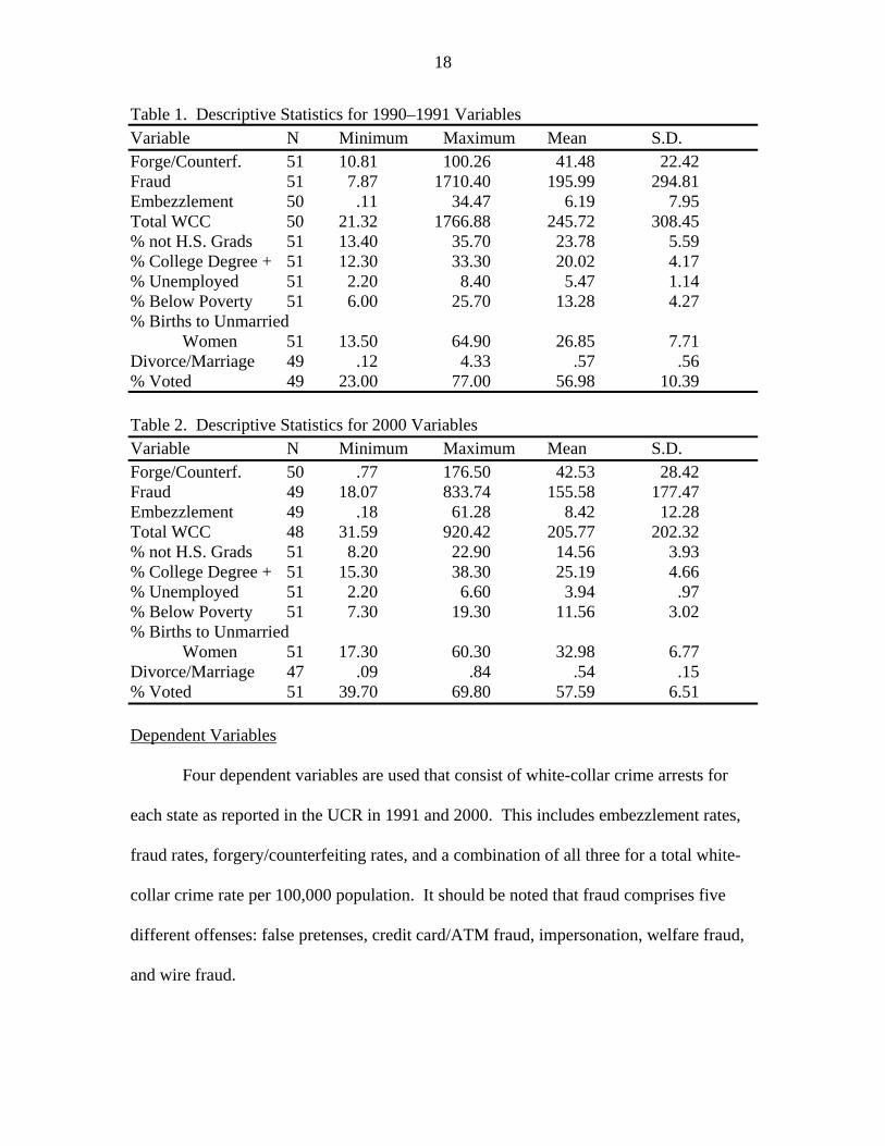
UCR and the Census. Tables 1 and 2 show descriptive statistics for the 1990–1991

variables and the 2000 variables, respectively.

17

18

Table 1. Descriptive Statistics for 1990–1991 Variables Variable N Minimum Maximum Mean S.D. Forge/Counterf. 51 10.81 100.26 41.48 22.42 Fraud 51 7.87 1710.40 195.99 294.81 Embezzlement 50 .11 34.47 6.19 7.95 Total WCC 50 21.32 1766.88 245.72 308.45 % not H.S. Grads 51 13.40 35.70 23.78 5.59 % College Degree + 51 12.30 33.30 20.02 4.17 % Unemployed 51 2.20 8.40 5.47 1.14 % Below Poverty 51 6.00 25.70 13.28 4.27 % Births to Unmarried Women 51 13.50 64.90 26.85 7.71 Divorce/Marriage 49 .12 4.33 .57 .56 % Voted 49 23.00 77.00 56.98 10.39 Table 2. Descriptive Statistics for 2000 Variables Variable N Minimum Maximum Mean S.D. Forge/Counterf. 50 .77 176.50 42.53 28.42 Fraud 49 18.07 833.74 155.58 177.47 Embezzlement 49 .18 61.28 8.42 12.28 Total WCC 48 31.59 920.42 205.77 202.32 % not H.S. Grads 51 8.20 22.90 14.56 3.93 % College Degree + 51 15.30 38.30 25.19 4.66 % Unemployed 51 2.20 6.60 3.94 .97 % Below Poverty 51 7.30 19.30 11.56 3.02 % Births to Unmarried Women 51 17.30 60.30 32.98 6.77 Divorce/Marriage 47 .09 .84 .54 .15 % Voted 51 39.70 69.80 57.59 6.51 Dependent Variables

Four dependent variables are used that consist of white-collar crime arrests for

each state as reported in the UCR in 1991 and 2000. This includes embezzlement rates,

fraud rates, forgery/counterfeiting rates, and a combination of all three for a total white-

collar crime rate per 100,000 population. It should be noted that fraud comprises five

different offenses: false pretenses, credit card/ATM fraud, impersonation, welfare fraud,

and wire fraud.

19

Independent Variables

The independent variables, gathered from the 1990 and 2000 Census Bureau’s

Statistical Abstract, measure each of the four institutions associated with IAT. Messner

and Rosenfeld are specific about the functions of each institution. For example, the

primary function of the family is to socialize and insulate its members by instilling the

values and skills that are necessary to combat the pressures created by the American

Dream; therefore, we can expect that disrupted families would be less adequate in

providing these necessary elements. Following Chamlin and Cochran (1995), family is

operationalized as the yearly divorce rate divided by the yearly marriage rate per 1,000

population (divorce/marriage ratio). Data on divorce and marriage rates were not

available in the 2000 Census Bureau’s Statistical Abstract, instead data was collected on

the 1998 divorce and marriage rates. The alternative model operationalization of family

disruption is measured as the percent of births to unmarried women. The alternative

measure of family is to ensure that the results are not sensitive to measurement decisions.

The second institution, education, functions to provide the tools necessary to

succeed later in life and to place the emphasis on knowledge rather than monetary

success. Thus, we expect that the lower the education level, the less one is equipped to

find alternative, legitimate ways to succeed. This is only the second study to ever look at

the education component of IAT. Following Piquero and Piquero (1998), education is

operationalized as the percent of the population that did not graduate from high school.

In order to be sure results are not sensitive to measurement decisions, an alternative

measure of education is utilized that examines the percent of the population with a

college degree or higher.

20

The third institution, polity, functions to maintain public safety and measures

society’s ability to take care of its members. As Messner and Rosenfeld (1997:1394)

suggest, it “reflects the quality as well as the quantity of social rights and entitlements.”

Therefore the polity is operationalized as the percent of registered voters who voted in the

1990 and 2000 elections; voting habits express citizens’ interest in society and their

ability to exercise their social rights.

Finally, IAT assumes that the American society is centered around economic

wealth and success; therefore, measures of economic deprivation would express the

inability of citizens to gain access to the American Dream through legitimate means. The

final institution, economy, is operationalized as the percent of the population that is

unemployed. Some may argue that the unemployment rate is an inadequate measure

because of the assumption that employment is a precondition of white-collar crime.

However, two points justify the use of this as a measure of economy. First, the UCR

relies upon offense-based measures of white-collar crime. Therefore, the acts defined as

white-collar crime do not rely on social status nor respectability requirements of white-

collar offenders. In other words, employment is not necessarily a pre-requisite for all

forms of white-collar crime (e.g., welfare fraud) including those used in these analyses.

Second, IAT is a macro-level theory that relies on rates as opposed to individual accounts

of behavior. Therefore, unemployment rates offer a measure of the overall economic

condition of the country. The alternative operationalization of economy is measured as

the percent of the population below the poverty level. This variable has been utilized in

previous in IAT studies by both Chamlin and Cochran (1995) and Piquero and Piquero

(1998).

21

Hypotheses

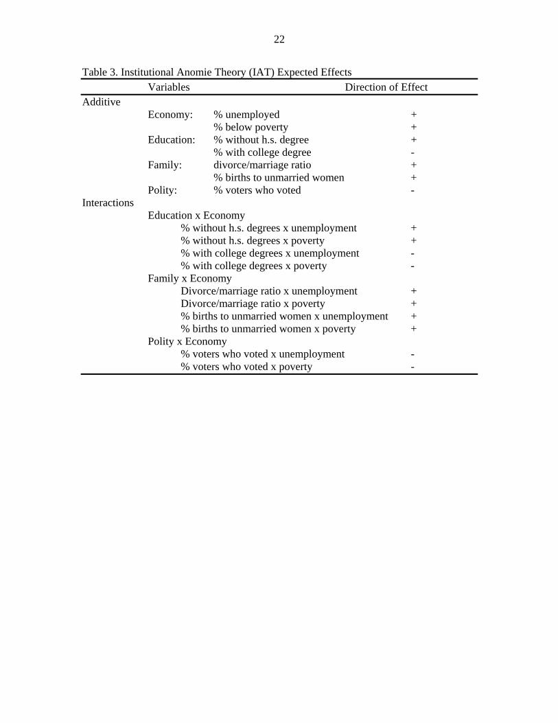
Using data gathered from the Census and FBI’s Uniform Crime Report, it is

expected that the results will be consistent with IAT predictions (Table 3). In other

words, it is expected that higher levels of voter participation (polity) will reduce the

crime rate. It is also expected that higher levels of family disruption (family), higher

levels of high school dropouts (education), and higher levels of unemployment

(economy) will increase the crime rate. Perhaps the most important characteristic of IAT

is the interaction effects of the economy with other non-economic institutions.

Consistent with IAT predictions, it is expected that lower percentages of the population

without high school degrees lessens the effect of unemployment on the white-collar crime

rate. It is also expected that lower divorce/marriage ratios (less divorces than marriages)

lessen the effect of unemployment on the white-collar crime rate. Finally, it is expected

that higher percentages of registered voters who voted lessens the effect of the economy

on white-collar crime rates. The question explored here is whether or not these same

predictions will hold for white-collar crimes.

Analytic Plan

To ascertain whether the assumptions put forth by IAT are also true in explaining

white-collar crime, a series of Poisson regressions was estimated. The out-come of

interest in the current analysis is the white-collar crime rate, defined as the number of

arrests divided by the size of the population. For many aggregate units, like states, the

offense rate is low relative to the population size, therefore the crime rate becomes less

precise and its distribution becomes skewed and discrete. To account for this problem,

Poisson based regression models are utilized in our study (Osgood, 2000).

22

Table 3. Institutional Anomie Theory (IAT) Expected Effects Variables Direction of Effect Additive Economy: % unemployed + % below poverty + Education: % without h.s. degree + % with college degree - Family: divorce/marriage ratio + % births to unmarried women + Polity: % voters who voted - Interactions Education x Economy % without h.s. degrees x unemployment + % without h.s. degrees x poverty + % with college degrees x unemployment - % with college degrees x poverty - Family x Economy Divorce/marriage ratio x unemployment + Divorce/marriage ratio x poverty + % births to unmarried women x unemployment + % births to unmarried women x poverty + Polity x Economy % voters who voted x unemployment - % voters who voted x poverty -

CHAPTER 4 RESULTS

Total White-Collar Crime Rates

In the first set of estimations, economy is measured as the percent of the

population unemployed, family is measured as the divorce/marriage ratio, polity is

measured as the percent of registered voters who voted, and education is measured as the

percent of the population without a high school degree. Estimates for the effects of the

independent variables on the total white-collar crime rate in 1991 are found in Model 1 of

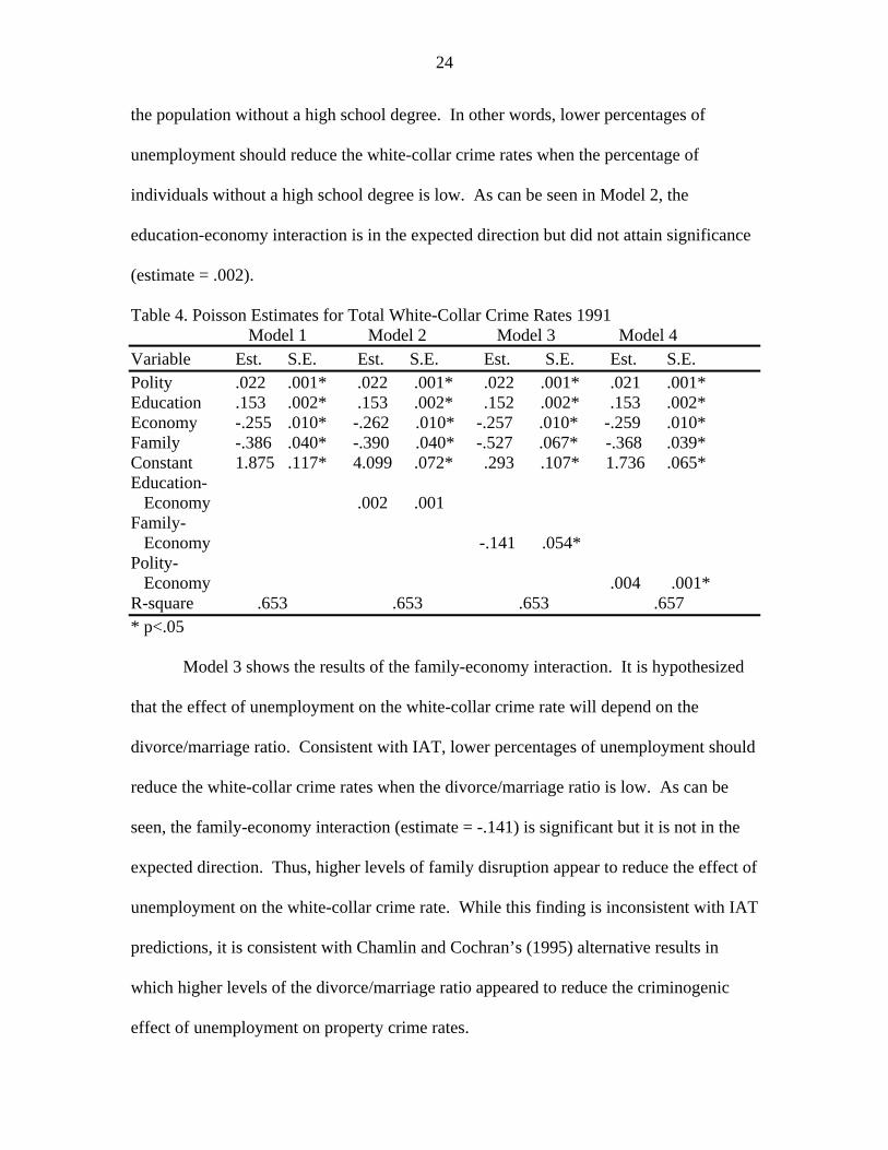
Table 4. All four independent variables attain significance; however, education is the

only variable in the expected direction. Both polity (estimate = .022) and education

(estimate = .153) exert positive effects on the total white-collar crime rate. Thus, higher

levels of voting and higher levels of the population without high school degrees, the

higher the white-collar crime rate. The economy (estimate = -.255) and family (estimate

= -.386) exert negative effects on the total white-collar crime rate; higher rates of

unemployment and higher levels of the divorce/marriage ratio (more divorces than

marriages) appear to reduce the white-collar crime rate.

Models 2 through 4 of Table 4 list the results of the interaction effects of the

economy with the other non-economic institutions. The additive effects remain

significant in all of the models with education still the only variable in the expected

direction. The first interaction term is education-economy. It is hypothesized that the

effect of unemployment on the white-collar crime rate will depend on the percentage of

23

24

the population without a high school degree. In other words, lower percentages of

unemployment should reduce the white-collar crime rates when the percentage of

individuals without a high school degree is low. As can be seen in Model 2, the

education-economy interaction is in the expected direction but did not attain significance

(estimate = .002).

Table 4. Poisson Estimates for Total White-Collar Crime Rates 1991 Model 1 Model 2 Model 3 Model 4 Variable Est. S.E. Est. S.E. Est. S.E. Est. S.E. Polity .022 .001* .022 .001* .022 .001* .021 .001* Education .153 .002* .153 .002* .152 .002* .153 .002* Economy -.255 .010* -.262 .010* -.257 .010* -.259 .010* Family -.386 .040* -.390 .040* -.527 .067* -.368 .039* Constant 1.875 .117* 4.099 .072* .293 .107* 1.736 .065* Education- Economy .002 .001 Family- Economy -.141 .054* Polity- Economy .004 .001* R-square .653 .653 .653 .657 * p<.05 Model 3 shows the results of the family-economy interaction. It is hypothesized

that the effect of unemployment on the white-collar crime rate will depend on the

divorce/marriage ratio. Consistent with IAT, lower percentages of unemployment should

reduce the white-collar crime rates when the divorce/marriage ratio is low. As can be

seen, the family-economy interaction (estimate = -.141) is significant but it is not in the

expected direction. Thus, higher levels of family disruption appear to reduce the effect of

unemployment on the white-collar crime rate. While this finding is inconsistent with IAT

predictions, it is consistent with Chamlin and Cochran’s (1995) alternative results in

which higher levels of the divorce/marriage ratio appeared to reduce the criminogenic

effect of unemployment on property crime rates.

25

Results of the polity-economy interaction can be found in Model 4. It is

hypothesized that the effect of unemployment on the white-collar crime rate will depend

on the percentage of registered voters who voted. Again, the interaction is significant but

it is not in the expected direction (estimate = .004). Inconsistent with IAT, lower levels

of voting appear to reduce the criminogenic effect of the economy on white-collar crime

rates.

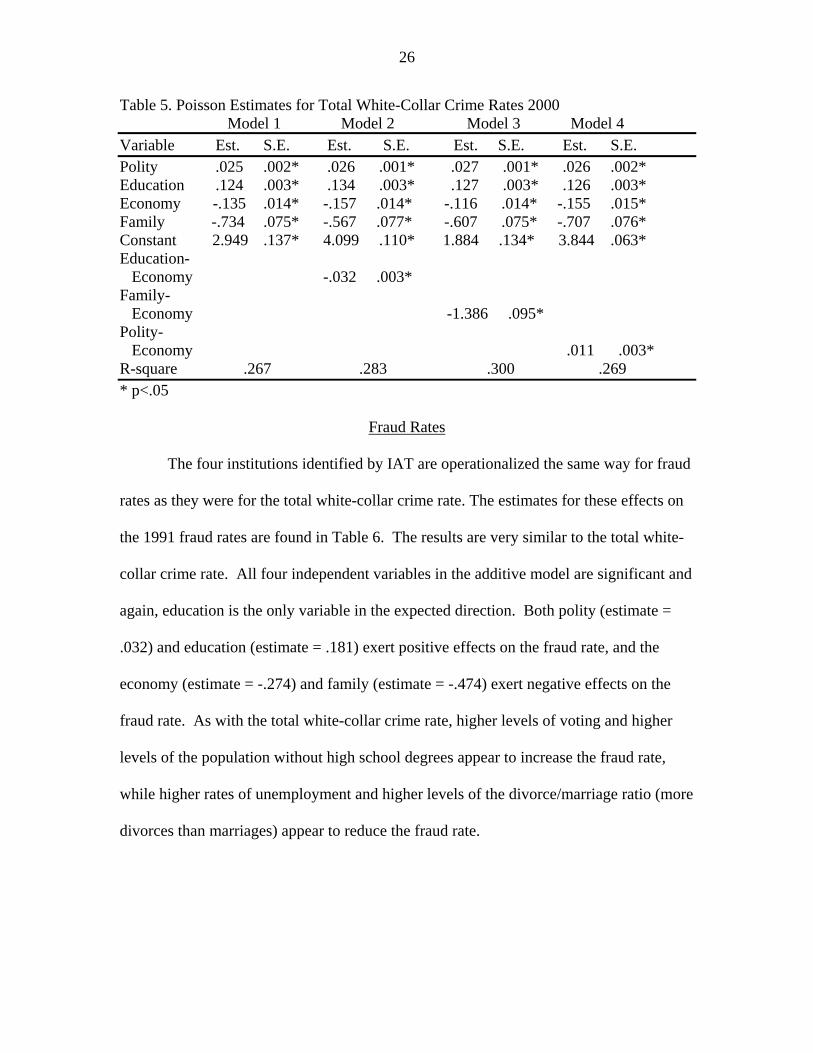
Results for the total white-collar crime rate in 2000 are similar to the results for

the 1991 crime rate (see Table 5) with regard to the additive effects. All four

independent variables in the additive model attain significance with education still the

only variable in the expected direction. Both polity (estimate = .025) and education

(estimate = .124) exert positive effects on the total white-collar crime rate, and the

economy (estimate = -.135) and family (estimate = -.734) exert negative effects on the

total white-collar crime rate. All three of the interaction terms (Models 2 through 4)

attain significance in predicting 2000 total white-collar crime rates. Family-economy

(estimate = -1.386) and polity-economy (estimate = .011) are both significant and again,

in the unexpected direction. Unlike the 1991 data, the education-economy interaction

attains significance in the 2000 data however, the sign also changes to the unexpected

direction. This suggests that higher percentages of the population without a high school

degree lessen the criminogenic effect of unemployment on the 2000 white-collar crime

rate.

26

Table 5. Poisson Estimates for Total White-Collar Crime Rates 2000 Model 1 Model 2 Model 3 Model 4 Variable Est. S.E. Est. S.E. Est. S.E. Est. S.E. Polity .025 .002* .026 .001* .027 .001* .026 .002* Education .124 .003* .134 .003* .127 .003* .126 .003* Economy -.135 .014* -.157 .014* -.116 .014* -.155 .015* Family -.734 .075* -.567 .077* -.607 .075* -.707 .076* Constant 2.949 .137* 4.099 .110* 1.884 .134* 3.844 .063* Education- Economy -.032 .003* Family- Economy -1.386 .095* Polity- Economy .011 .003* R-square .267 .283 .300 .269 * p<.05

Fraud Rates

The four institutions identified by IAT are operationalized the same way for fraud

rates as they were for the total white-collar crime rate. The estimates for these effects on

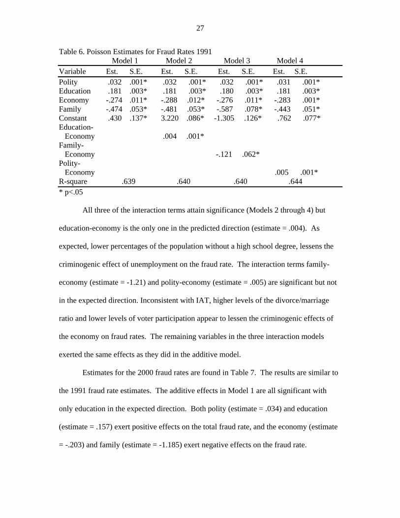
the 1991 fraud rates are found in Table 6. The results are very similar to the total white-

collar crime rate. All four independent variables in the additive model are significant and

again, education is the only variable in the expected direction. Both polity (estimate =

.032) and education (estimate = .181) exert positive effects on the fraud rate, and the

economy (estimate = -.274) and family (estimate = -.474) exert negative effects on the

fraud rate. As with the total white-collar crime rate, higher levels of voting and higher

levels of the population without high school degrees appear to increase the fraud rate,

while higher rates of unemployment and higher levels of the divorce/marriage ratio (more

divorces than marriages) appear to reduce the fraud rate.

27

Table 6. Poisson Estimates for Fraud Rates 1991 Model 1 Model 2 Model 3 Model 4 Variable Est. S.E. Est. S.E. Est. S.E. Est. S.E. Polity .032 .001* .032 .001* .032 .001* .031 .001* Education .181 .003* .181 .003* .180 .003* .181 .003* Economy -.274 .011* -.288 .012* -.276 .011* -.283 .001* Family -.474 .053* -.481 .053* -.587 .078* -.443 .051* Constant .430 .137* 3.220 .086* -1.305 .126* .762 .077* Education- Economy .004 .001* Family- Economy -.121 .062* Polity- Economy .005 .001* R-square .639 .640 .640 .644 * p<.05 All three of the interaction terms attain significance (Models 2 through 4) but

education-economy is the only one in the predicted direction (estimate = .004). As

expected, lower percentages of the population without a high school degree, lessens the

criminogenic effect of unemployment on the fraud rate. The interaction terms family-

economy (estimate = -1.21) and polity-economy (estimate = .005) are significant but not

in the expected direction. Inconsistent with IAT, higher levels of the divorce/marriage

ratio and lower levels of voter participation appear to lessen the criminogenic effects of

the economy on fraud rates. The remaining variables in the three interaction models

exerted the same effects as they did in the additive model.

Estimates for the 2000 fraud rates are found in Table 7. The results are similar to

the 1991 fraud rate estimates. The additive effects in Model 1 are all significant with

only education in the expected direction. Both polity (estimate = .034) and education

(estimate = .157) exert positive effects on the total fraud rate, and the economy (estimate

= -.203) and family (estimate = -1.185) exert negative effects on the fraud rate.

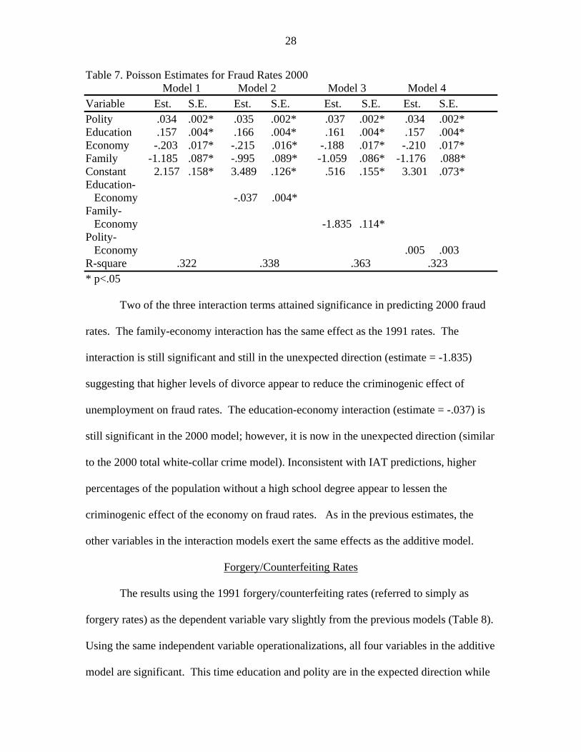
28

Table 7. Poisson Estimates for Fraud Rates 2000 Model 1 Model 2 Model 3 Model 4 Variable Est. S.E. Est. S.E. Est. S.E. Est. S.E. Polity .034 .002* .035 .002* .037 .002* .034 .002* Education .157 .004* .166 .004* .161 .004* .157 .004* Economy -.203 .017* -.215 .016* -.188 .017* -.210 .017* Family -1.185 .087* -.995 .089* -1.059 .086* -1.176 .088* Constant 2.157 .158* 3.489 .126* .516 .155* 3.301 .073* Education- Economy -.037 .004* Family- Economy -1.835 .114* Polity- Economy .005 .003 R-square .322 .338 .363 .323 * p<.05

Two of the three interaction terms attained significance in predicting 2000 fraud

rates. The family-economy interaction has the same effect as the 1991 rates. The

interaction is still significant and still in the unexpected direction (estimate = -1.835)

suggesting that higher levels of divorce appear to reduce the criminogenic effect of

unemployment on fraud rates. The education-economy interaction (estimate = -.037) is

still significant in the 2000 model; however, it is now in the unexpected direction (similar

to the 2000 total white-collar crime model). Inconsistent with IAT predictions, higher

percentages of the population without a high school degree appear to lessen the

criminogenic effect of the economy on fraud rates. As in the previous estimates, the

other variables in the interaction models exert the same effects as the additive model.

Forgery/Counterfeiting Rates

The results using the 1991 forgery/counterfeiting rates (referred to simply as

forgery rates) as the dependent variable vary slightly from the previous models (Table 8).

Using the same independent variable operationalizations, all four variables in the additive

model are significant. This time education and polity are in the expected direction while

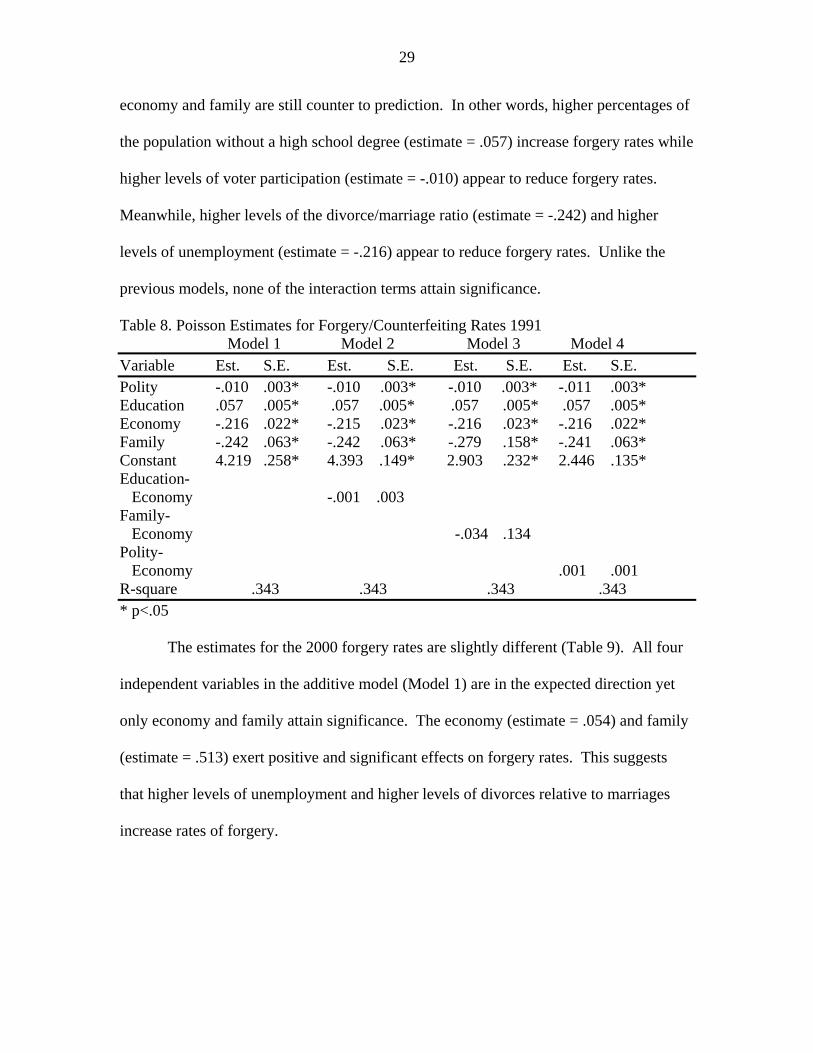
29

economy and family are still counter to prediction. In other words, higher percentages of

the population without a high school degree (estimate = .057) increase forgery rates while

higher levels of voter participation (estimate = -.010) appear to reduce forgery rates.

Meanwhile, higher levels of the divorce/marriage ratio (estimate = -.242) and higher

levels of unemployment (estimate = -.216) appear to reduce forgery rates. Unlike the

previous models, none of the interaction terms attain significance.

Table 8. Poisson Estimates for Forgery/Counterfeiting Rates 1991 Model 1 Model 2 Model 3 Model 4 Variable Est. S.E. Est. S.E. Est. S.E. Est. S.E. Polity -.010 .003* -.010 .003* -.010 .003* -.011 .003* Education .057 .005* .057 .005* .057 .005* .057 .005* Economy -.216 .022* -.215 .023* -.216 .023* -.216 .022* Family -.242 .063* -.242 .063* -.279 .158* -.241 .063* Constant 4.219 .258* 4.393 .149* 2.903 .232* 2.446 .135* Education- Economy -.001 .003 Family- Economy -.034 .134 Polity- Economy .001 .001 R-square .343 .343 .343 .343 * p<.05

The estimates for the 2000 forgery rates are slightly different (Table 9). All four

independent variables in the additive model (Model 1) are in the expected direction yet

only economy and family attain significance. The economy (estimate = .054) and family

(estimate = .513) exert positive and significant effects on forgery rates. This suggests

that higher levels of unemployment and higher levels of divorces relative to marriages

increase rates of forgery.

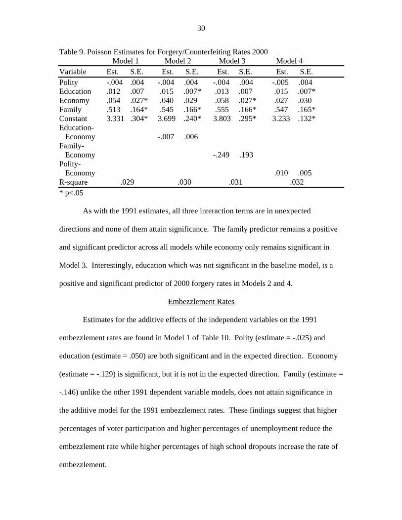
30

Table 9. Poisson Estimates for Forgery/Counterfeiting Rates 2000 Model 1 Model 2 Model 3 Model 4 Variable Est. S.E. Est. S.E. Est. S.E. Est. S.E. Polity -.004 .004 -.004 .004 -.004 .004 -.005 .004 Education .012 .007 .015 .007* .013 .007 .015 .007* Economy .054 .027* .040 .029 .058 .027* .027 .030 Family .513 .164* .545 .166* .555 .166* .547 .165* Constant 3.331 .304* 3.699 .240* 3.803 .295* 3.233 .132* Education- Economy -.007 .006 Family- Economy -.249 .193 Polity- Economy .010 .005 R-square .029 .030 .031 .032 * p<.05

As with the 1991 estimates, all three interaction terms are in unexpected

directions and none of them attain significance. The family predictor remains a positive

and significant predictor across all models while economy only remains significant in

Model 3. Interestingly, education which was not significant in the baseline model, is a

positive and significant predictor of 2000 forgery rates in Models 2 and 4.

Embezzlement Rates

Estimates for the additive effects of the independent variables on the 1991

embezzlement rates are found in Model 1 of Table 10. Polity (estimate = -.025) and

education (estimate = .050) are both significant and in the expected direction. Economy

(estimate = -.129) is significant, but it is not in the expected direction. Family (estimate =

-.146) unlike the other 1991 dependent variable models, does not attain significance in

the additive model for the 1991 embezzlement rates. These findings suggest that higher

percentages of voter participation and higher percentages of unemployment reduce the

embezzlement rate while higher percentages of high school dropouts increase the rate of

embezzlement.

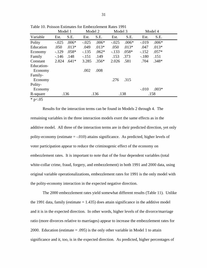
31

Table 10. Poisson Estimates for Embezzlement Rates 1991 Model 1 Model 2 Model 3 Model 4 Variable Est. S.E. Est. S.E. Est. S.E. Est. S.E. Polity -.025 .006* -.025 .006* -.025 .006* -.019 .006* Education .050 .013* .049 .013* .050 .013* .047 .013* Economy -.129 .058* -.135 .062* -.133 .058* -.152 .057* Family -.146 .148 -.151 .149 .153 .373 -.180 .151 Constant 2.824 .641* 3.285 .356* 2.026 .581 .704 .348* Education- Economy .002 .008 Family- Economy .276 .315 Polity- Economy -.010 .003* R-square .136 .136 .138 .158 * p<.05 Results for the interaction terms can be found in Models 2 through 4. The

remaining variables in the three interaction models exert the same effects as in the

additive model. All three of the interaction terms are in their predicted direction, yet only

polity-economy (estimate = -.010) attains significance. As predicted, higher levels of

voter participation appear to reduce the criminogenic effect of the economy on

embezzlement rates. It is important to note that of the four dependent variables (total

white-collar crime, fraud, forgery, and embezzlement) in both 1991 and 2000 data, using

original variable operationalizations, embezzlement rates for 1991 is the only model with

the polity-economy interaction in the expected negative direction.

The 2000 embezzlement rates yield somewhat different results (Table 11). Unlike

the 1991 data, family (estimate = 1.435) does attain significance in the additive model

and it is in the expected direction. In other words, higher levels of the divorce/marriage

ratio (more divorces relative to marriages) appear to increase the embezzlement rates for

2000. Education (estimate = .095) is the only other variable in Model 1 to attain

significance and it, too, is in the expected direction. As predicted, higher percentages of

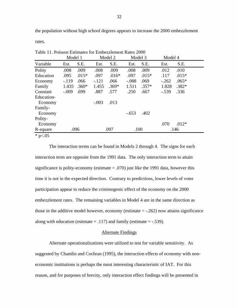
32

the population without high school degrees appears to increase the 2000 embezzlement

rates.

Table 11. Poisson Estimates for Embezzlement Rates 2000 Model 1 Model 2 Model 3 Model 4 Variable Est. S.E. Est. S.E. Est. S.E. Est. S.E. Polity .008 .009 .008 .009 .008 .009 .012 .010 Education .095 .015* .097 .016* .097 .015* .117 .015* Economy -.119 .066 -.121 .066 -.088 .069 -.262 .065* Family 1.435 .360* 1.455 .369* 1.511 .357* 1.828 .382* Constant -.009 .699 .887 .577 .250 .667 -.539 .336 Education- Economy -.003 .013 Family- Economy -.653 .402 Polity- Economy .070 .012* R-square .096 .097 .100 .146 * p<.05 The interaction terms can be found in Models 2 through 4. The signs for each

interaction term are opposite from the 1991 data. The only interaction term to attain

significance is polity-economy (estimate = .070) just like the 1991 data, however this

time it is not in the expected direction. Contrary to predictions, lower levels of voter

participation appear to reduce the criminogenic effect of the economy on the 2000

embezzlement rates. The remaining variables in Model 4 are in the same direction as

those in the additive model however, economy (estimate = -.262) now attains significance

along with education (estimate = .117) and family (estimate = -.539).

Alternate Findings

Alternate operationalizations were utilized to test for variable sensitivity. As

suggested by Chamlin and Cochran (1995), the interaction effects of economy with non-

economic institutions is perhaps the most interesting characteristic of IAT. For this

reason, and for purposes of brevity, only interaction effect findings will be presented in

33

this section. However, complete tables showing results for all models can be found in the

Appendix.

In the first alternate model, economy is measured as the percent of the population

unemployed, education is measured as the percent of the population without a high

school degree, polity is measured as the percent of registered voters who voted, and the

alternate measure of family is operationalized as the percent of births to unmarried

women. Results for 1991 are found in Tables A-1 through A-4 in the Appendix.

The family-economy interaction (estimate = -.013) exerts a negative and

significant effect on the 1991 total white-collar crime rate. Contrary to IAT, it still

appears as though higher levels of family disruption (percent of births to unmarried

women) reduce the effects of unemployment in the 1991 total white-collar crime rate.

The same results are seen when looking at the 1991 fraud rates; the alternate family-

economy interaction (estimate = -.018) continues to exert a negative and significant effect

(Table A-2).

The polity-economy interaction in the alternate family model for the 1991 total

white-collar crime rate also exerts the same effects as the original model. Again, the

interaction is significant but is not in the expected direction (estimate = .003).

Inconsistent with IAT predictions, lower levels of voting appear to reduce the

criminogenic effect of the economy on the total white-collar crime rate. The same

appears to be true for the 1991 fraud rates. Meanwhile, the polity-economy interaction in

the alternate family model changes to the expected direction for the embezzlement rate

estimates (Table A-4) suggesting that higher levels of voting appear to reduce the

criminogenic effect of the economy on 1991 embezzlement rates.

34

The alternate family estimates exert similar effects on the 2000 data as in the

original 2000 estimations. Results for the alternate family operationalizations are found

in Tables A-5 through A-8 in the Appendix. Both the education-economy interaction and

the family-economy interactions, counter to expectation, exert negative effects on all four

crime types; however, both interactions only attain significance in the 2000 total white-

collar crime rate and the 2000 fraud rate models. Thus, higher percentages of the

population without high school degrees and higher percentages of births to unmarried

women appear to reduce the criminogenic effect of the economy on both the 2000 total

white-collar crime rates and the 2000 fraud rates.

The final interaction term in the alternate family model, polity-economy is

different from the original model. The interaction exerts negative effects on both the

2000 total white-collar crime rate and the 2000 fraud rate but it only attains significance

in the 2000 fraud rate model. Consistent with IAT, higher levels of voting appear to

reduce the criminogenic effect of unemployment on the 2000 fraud rates.

The second alternate model operationalizes economy as the percent of the

population below the poverty level. Results for the 1991 are found in Table B-1 through

B-4 in the Appendix. Table B-1 presents the 1991 total white-collar crime rate estimates.

The interaction terms in the alternate economy model are consistent with the original

model except that the education-economy interaction (estimate = .002) attains

significance when economy is operationalized as the percent of the population below the

poverty level (Table B-1). As predicted, lower percentages of the population without

high school degrees appears to reduce the criminogenic effect of poverty on the 1991

total white-collar crime rate. The same results are seen in the fraud and forgery rates for

35

1991 (Tables B-2 and B-3). As with the original model, the family-economy interaction

(estimate = -.286) exerts a negative and significant effect suggesting that lower levels of

the divorce/marriage ratio appear to reduce the effect of poverty on the total white-collar

crime rate. Similar results are found for the fraud and forgery rates for 1991 (Tables B-2

and B-3). Finally, the polity-economy interaction (estimate = .002) also exerts an

unexpected, positive and significant effect indicating that lower percentages of voter

participation appear to reduce the effect of poverty on the crime rate. The same is true

for the 1991 fraud rates (Table B-2).

The polity-economy interaction for 1991 forgery rates remains significant

however, the sign changes (estimate = -.001). Consistent with IAT predictions, higher

percentages of voter participation in elections appear to reduce the criminogenic effect of

poverty on forgery rates. The same result is found in the 1991 embezzlement model.

The interaction terms for the 1991 embezzlement rates seem to have the opposite

effect as seen in the other models (Table B-4). The family-economy interaction does

however, exert a positive and significant effect suggesting that lower levels of family

disruption appear to reduce the criminogenic effect of poverty on embezzlement rates.

This finding is consistent with IAT.

Interactions for the alternate economy measure in the 2000 total white-collar

crime data are different from the 1991 data (Table B-5). While all three interactions

remain significant, the signs for education-economy and polity-economy have changed.

Using 2000 data, results indicate that lower levels of education appear to reduce the

effect of poverty on the total white-collar crime rate, higher levels of voter participation

and higher levels of family disruption also appear to reduce the effect of poverty. The

36

polity-economy interaction is the only interaction consistent with IAT predictions. The

same results are seen in the estimates for the 2000 fraud rate (Table B-6).

Just as the forgery and embezzlement estimates deviated in the 1991 data, they

deviate again in the 2000 data. In the 2000 forgery rate estimations (Table B-7), the only

interaction to attain significance is family-economy and it is in the unexpected direction

indicating that higher levels of family disruption appear to reduce the effect of poverty on

forgery rates. The interaction term, education-economy, for the 2000 embezzlement rates

is similar to the total white-collar crime rate findings; it exerts a significant, yet

unexpected negative effect on embezzlement indicating that higher percentages of the

population without high school degrees appear to reduce the effect of poverty on

embezzlement (Table B-8). Finally, the polity-economy interaction is significant but it is

in the unexpected direction. Inconsistent with IAT, it appears as though lower levels of

voter participation reduce the effect of poverty on the 2000 embezzlement rates.

The final alternate model testing for sensitivity operationalizes education as the

percent of the population with a college degree or more. Economy is still measured as

the percent of the population unemployed, family is measured as the divorce/marriage

ratio, and the polity is measured as the percent of registered voters who voted. It is

important to note that the new education variable is expected to exert the opposite effect

on the crime rates that the original measure did. In other words, IAT predicts that higher

levels of education would work to reduce crime rates, therefore, lower levels of

individuals without high school degrees (positive effect) and higher levels of individuals

with college degrees (negative effect) should both work to reduce crime rates.

37

The estimates for the 1991 total white-collar crime rates using the alternate

education variable are found in Table C-1 in the Appendix. The interaction term

education-economy (estimate = -.030) exerts a negative and significant effect. As

predicted, higher levels of education appear to reduce the criminogenic effects of the

economy on the white-collar crime rate. This finding is also present when looking at

estimates for the 1991 fraud rate (Table C-2). Counter to prediction, the education-

economy interaction exerts a positive and significant effect on the 1991 forgery rates,

indicating that lower percentages of the population with college degrees or more appear

to reduce forgery rates (Table C-3).

The next interaction term, family-economy, exerts a negative and significant

effect on the 1991 total white-collar crime rate. Contrary to predictions, it appears as

though higher levels of family disruption reduce the effects of unemployment. The same

results are found in the estimates for the 1991 fraud rates.

The final interaction term in the alternate education model, polity-economy,

exerts a positive and significant effect on the 1991 total white-collar crime rates

indicating that lower levels of voter participation appear to reduce the effects of the

economy on the white-collar crime rate. Again, this finding is reproduced in estimates

for 1991 fraud rates. Finally, the interaction exerts a negative and significant effect on

the 1991 embezzlement rate (Tables C-5 through C-8). Consistent with predictions,

higher levels of voter participation appear to reduce the effects of the economy on the

1991 embezzlement rates.

The education-economy interaction, still using the alternate measure of education,

exerts a positive and significant effect on the 2000 total white-collar crime rate (Table C-

38

5). Contrary to predictions, lower percentages of the population with college degrees or

more appear to reduce the effect of the economy in the total white-collar crime rate. This

same finding is also present in the estimates for the 2000 fraud rates and the 2000 forgery

rates (Tables C-6 and C-7). As predicted, the interaction does exert a negative and

significant effect on the 2000 embezzlement rates indicating that higher levels of

education appear to reduce the effects of the economy on embezzlement rates (Table C-

8).

The second interaction term in the alternate education model for the 2000 data is

family-economy. This interaction exerts an unexpected negative effect on all four

dependent variable estimations suggesting that higher levels of family disruption actually

reduce the crime rate. However, the interaction term is only significant in the total white-

collar crime and fraud estimates.

The final interaction term is polity-economy and it, too, exerts an unexpected

positive and significant effect on all four dependent variable models. Thus, contrary to

IAT, lower levels of voter participation appear to reduce the criminogenic effect of

unemployment on the total white-collar crime rate, forgery rate, fraud rate, and

embezzlement rate for the year 2000.

CHAPTER 5 DISCUSSION AND CONCLUSION

Discussion

This paper set out to examine the relationship between IAT and white-collar

crime, specifically UCR measures of fraud, embezzlement, forgery and counterfeiting,

and a combination of all three, the total white-collar crime rate. Using Census data to

measure key IAT variables, the results show mixed support for the theory.

In the additive fashion, education in both the original and alternate models, lends

support for all but two of the dependent variable estimations (1991 alternate family

estimates for embezzlement and the 2000 alternate family estimates for forgery). As

predicted, lower percentages of the population without high school degrees and higher

percentages of the population with college degrees or more appear to reduce white-collar

crime rates.

Mixed support is also observed in the interaction terms for both

operationalizations of education-economy. The interaction seems to receive the most

support for IAT in the 1991 alternate economy estimations. However, support from the

interaction seems to be evenly split among all dependent variable estimations.

Family, measured as the divorce/marriage ratio, shows support for IAT in the

additive models only in estimations of the 2000 data for forgery and embezzlement

(including the alternate education and alternate economy models). Contrary to IAT, the

remaining models, and all but one interaction model (1991 alternate economy

39

40

embezzlement rates), indicate that higher levels of family disruption (more divorces than

marriages) actually appear to reduce white-collar crime rates. There could be several

reasons for this contradictory finding. First, there may be other factors involved, or it

may simply be that the divorce/marriage ratio is an inadequate measure of family

disruption. In fact, divorce itself may not be the signature of family disruption; rather,

divorce could be seen as a means to an end of family disruption. Similarly, just because a

couple refrains from divorce does not mean there is no family disruption. If this were the

case, divorce could be interpreted as an end to family disruption thereby exerting a

negative rather than positive effect. Then, the data would show overwhelming support

for IAT in the family-economy interaction terms.

However, when family disruption is operationalized as the percent of births to

unmarried women, the additive results, for the most part, support IAT; as hypothesized,

lower levels of family disruption, in the form of births to unmarried women, appear to

reduce white-collar crime rates in both the 1991 and 2000 data. The family-economy

interactions in the alternate family models do not support IAT; in fact, they suggest that

higher percentages of births to unmarried women may actually work to reduce white-

collar crime rates. While it could be argued that single mothers may be more likely to

engage in white-collar crimes to acquire money to better care for their children, it could

also be argued that single mothers would be more likely to refrain from engaging in

white-collar offenses because consequences of losing their job would hinder their ability

to care for their children. Either way you look at it, support for IAT is mixed.

As with the other variables, results show mixed support for IAT when

operationalizing polity as the percent of registered voters who voted in elections. Polity

41

receives the most additive support in the 1991 alternate education models, where it is

significant and in the hypothesized direction for all four dependent variable estimations.

Therefore, in the 1991 alternate education models, it appears as though higher

percentages of voter participation reduce white-collar crime rates. Polity-economy

interaction effects are also mixed. One quarter of the estimation models appear to

support IAT; higher levels of voter participation appear to reduce the criminogenic effect

of the economy on white-collar crime rates. The remaining models do not appear to

support IAT; lower levels of voter participation appear to reduce the criminogenic effect

of the economy on white-collar crime rates.

The final variable, economy, measured as the percent of the population

unemployed, produces very little support for IAT in the additive models. For the most

part, results indicate that higher levels of unemployment appear to reduce white-collar

crime rates. However, if we accept the unemployment rate as a measure of opportunity, a

key component of white-collar offending (Coleman, 1994) rather than as an indicator of a

poor economy, the results seem to make sense. The lower the employment rate, the less

opportunities there are to engage in white-collar offending. While this finding does not

support IAT, it does however make intuitive sense. The alternate measure of economy,

the percent of the population below the poverty level also produces mixed support for the

theory.

Limitations and Future Research

As with all research, our study was not without limitations. First, IAT is a

complicated theory to test, specifically because there are no clear indicators of how to

measure the four social institutions. This being the first test of IAT and white-collar

42

crime was especially difficult. This paper used variables that had been successfully

applied in previous IAT studies on property crime and violent crime; the question raised

is whether or not these same variables could explain white-collar offending. As with the

previous studies though, results show mixed support. Also, there are no measures of

anomie or culture; our study assumes that everyone buys into the American Dream. It

has been suggested that the inclusion of cultural variables might reduce the economic and

non-economic variables to nothing more than control variables (Piquero and Piquero,

1998). However, as suggested, measuring culture and anomie is perhaps “the most

difficult problem facing researchers who are interested in testing IAT” (Piquero and

Piquero, 1998:80).

A second limitation to our study lies in the interpretation of the variables. For

purposes of our study it was assumed that divorce was a measure of family disruption

when in fact divorce could be interpreted as an end to family disruption. Even though it

is the same variable, we would expect the two interpretations to exert opposite effects on

the crime rate. The same is true when measuring economy as the unemployment rate; the

results did not necessarily support IAT, but they made sense. Perhaps unemployment is

more a measure of opportunity than it is of economic conditions when dealing with

white-collar crime variables. In other words, misinterpretation of what the variables

actually measure creates a problem when determining support, or lack thereof, for the

theory.

Finally, the measurement of the dependent variables is a limitation to our study.

As discussed earlier, there are many criticisms about using UCR data to measure white-

collar crime. Perhaps the biggest criticism is that the typical fraud and forgery offenders

43

(as measured by the UCR) commit non-occupational crimes. This is especially

troublesome because it is obvious in our study that the fraud estimates are driving the

total white-collar crime rate estimates. Embezzlement rates, on the other hand do fit the

broad definition for white-collar offenses even though arrests are few. For these reasons,

each UCR white-collar crime measure was tested separately and as a group in our study.

In all instances, support for IAT was still mixed. Even with its limitation, researchers

continue to use UCR data for white-collar crime studies because of the lack of other data

sources that measure white-collar offending so uniformly.

Future research using more accurate measures of white-collar crime is necessary

to further the scope of IAT. Successful nationwide participation in the FBI’s National

Incident-Based Reporting System (NIBRS) would help to alleviate the issue of non-

occupational and occupational offending in the current white-collar crime measures. As

opposed to the UCR’s offense-based reports, NIBRS will take into account characteristics

of the crime and the offender. Measures of corporate offending and regulatory and civil

violations should also be included in later studies. While opportunity is not specifically

measured in our study, it is indirectly touched upon through the use of unemployment

variable. Opportunity is a key component to white-collar offending and therefore future

studies should attempt to control for this measure. Future research also needs to focus

more on appropriate institutional operationalizations that limit the possible interpretations

of variables. Finally, control variables appropriate for white-collar crime also need to be

included in future studies of institutional anomie theory and white-collar crime.

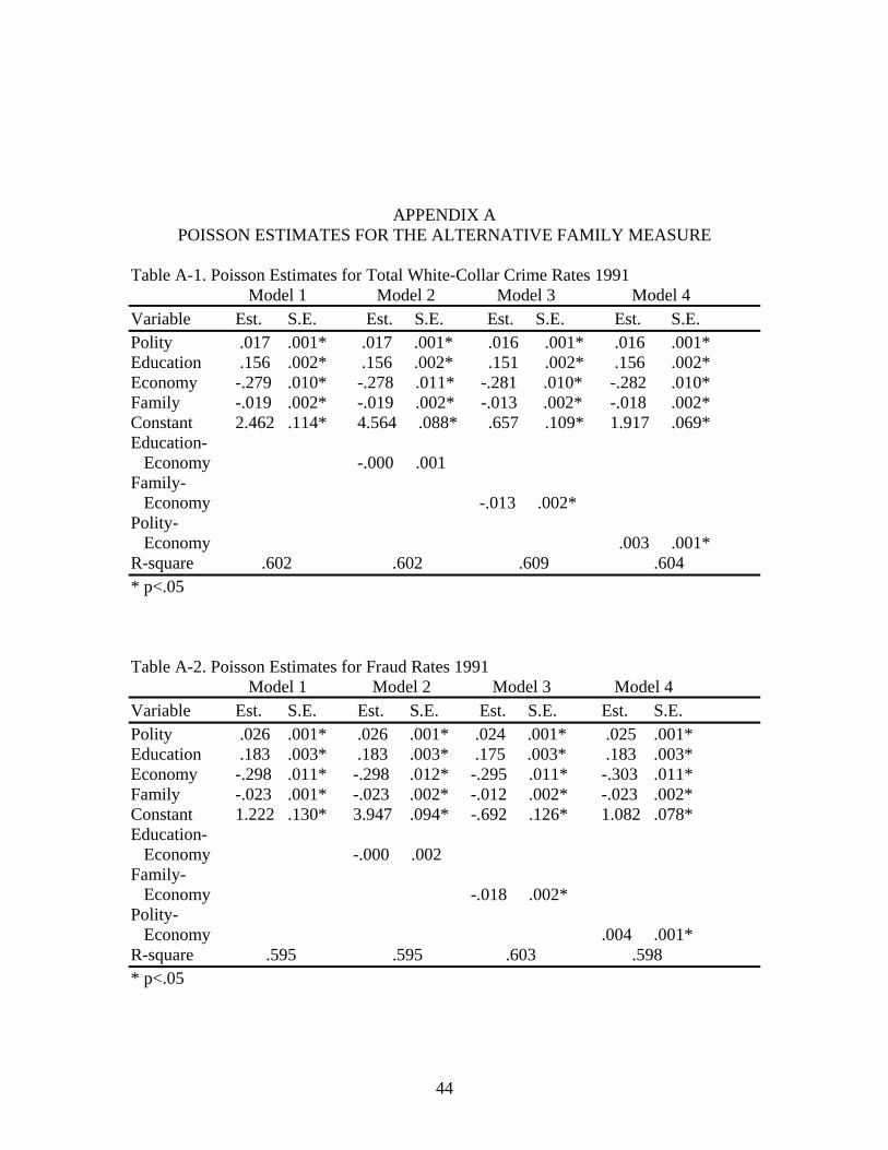
APPENDIX A POISSON ESTIMATES FOR THE ALTERNATIVE FAMILY MEASURE

Table A-1. Poisson Estimates for Total White-Collar Crime Rates 1991 Model 1 Model 2 Model 3 Model 4 Variable Est. S.E. Est. S.E. Est. S.E. Est. S.E. Polity .017 .001* .017 .001* .016 .001* .016 .001* Education .156 .002* .156 .002* .151 .002* .156 .002* Economy -.279 .010* -.278 .011* -.281 .010* -.282 .010* Family -.019 .002* -.019 .002* -.013 .002* -.018 .002* Constant 2.462 .114* 4.564 .088* .657 .109* 1.917 .069* Education- Economy -.000 .001 Family- Economy -.013 .002* Polity- Economy .003 .001* R-square .602 .602 .609 .604 * p<.05 Table A-2. Poisson Estimates for Fraud Rates 1991 Model 1 Model 2 Model 3 Model 4 Variable Est. S.E. Est. S.E. Est. S.E. Est. S.E. Polity .026 .001* .026 .001* .024 .001* .025 .001* Education .183 .003* .183 .003* .175 .003* .183 .003* Economy -.298 .011* -.298 .012* -.295 .011* -.303 .011* Family -.023 .001* -.023 .002* -.012 .002* -.023 .002* Constant 1.222 .130* 3.947 .094* -.692 .126* 1.082 .078* Education- Economy -.000 .002 Family- Economy -.018 .002* Polity- Economy .004 .001* R-square .595 .595 .603 .598 * p<.05

44

45

Table A-3. Poisson Estimates for Forgery/Counterfeiting Rates 1991 Model 1 Model 2 Model 3 Model 4 Variable Est. S.E. Est. S.E. Est. S.E. Est. S.E. Polity -.009 .002* -.009 .002* -.008 .002* -.010 .002* Education .055 .005* .055 .005* .058 .006* .056 .005* Economy -.233 .023* -.233 .023* -.229 .023* -.233 .023* Family .012 .003* .012 .003* .008 .004* .012 .003* Constant 3.803 .247* 3.845 .163* 2.750 .244* 2.005 .137* Education- Economy .000 .003 Family- Economy .004 .003 Polity- Economy .001 .001 R-square .328 .328 .330 .329 * p<.05 Table A-4. Poisson Estimates for Embezzlement Rates 1991 Model 1 Model 2 Model 3 Model 4 Variable Est. S.E. Est. S.E. Est. S.E. Est. S.E. Polity -.028 .006* -.027 .006* -.024 .006* -.022 .006* Education .025 .015 .024 .015 .030 .015 .027 .015 Economy -.166 .061* -.171 .063* -.166 .060* -.181 .059* Family .038 .013* .038 .013* .030 .014* .030 .013* Constant 2.644 .656* 2.297 .517* 2.415 .628* .285 .388 Education- Economy .002 .008 Family- Economy .012 .008 Polity- Economy -.009 .003* R-square .147 .147 .152 .162 * p<.05

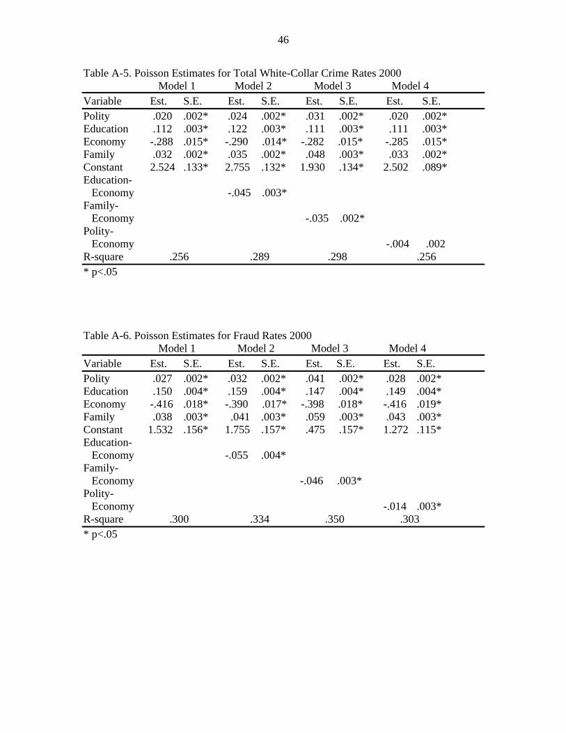
46

Table A-5. Poisson Estimates for Total White-Collar Crime Rates 2000 Model 1 Model 2 Model 3 Model 4 Variable Est. S.E. Est. S.E. Est. S.E. Est. S.E. Polity .020 .002* .024 .002* .031 .002* .020 .002* Education .112 .003* .122 .003* .111 .003* .111 .003* Economy -.288 .015* -.290 .014* -.282 .015* -.285 .015* Family .032 .002* .035 .002* .048 .003* .033 .002* Constant 2.524 .133* 2.755 .132* 1.930 .134* 2.502 .089* Education- Economy -.045 .003* Family- Economy -.035 .002* Polity- Economy -.004 .002 R-square .256 .289 .298 .256 * p<.05 Table A-6. Poisson Estimates for Fraud Rates 2000 Model 1 Model 2 Model 3 Model 4 Variable Est. S.E. Est. S.E. Est. S.E. Est. S.E. Polity .027 .002* .032 .002* .041 .002* .028 .002* Education .150 .004* .159 .004* .147 .004* .149 .004* Economy -.416 .018* -.390 .017* -.398 .018* -.416 .019* Family .038 .003* .041 .003* .059 .003* .043 .003* Constant 1.532 .156* 1.755 .157* .475 .157* 1.272 .115* Education- Economy -.055 .004* Family- Economy -.046 .003* Polity- Economy -.014 .003* R-square .300 .334 .350 .303 * p<.05

47

Table A-7. Poisson Estimates for Forgery/Counterfeiting Rates 2000 Model 1 Model 2 Model 3 Model 4 Variable Est. S.E. Est. S.E. Est. S.E. Est. S.E. Polity -.003 .004 -.002 .004 -.001 .004 -.003 .004 Education .001 .007 .004 .008 .002 .007 .003 .007 Economy .042 .026 .032 .028 .038 .026 .031 .028 Family .014 .005* .015 .005* .016 .005* .013 .005* Constant 3.228 .281* 3.388 .264* 3.802 .279* 3.248 .150* Education- Economy -.005 .006 Family- Economy -.005 .004 Polity- Economy .005 .005 R-square .024 .025 .025 .025 * p<.05 Table A-8. Poisson Estimates for Embezzlement Rates 2000 Model 1 Model 2 Model 3 Model 4 Variable Est. S.E. Est. S.E. Est. S.E. Est. S.E. Polity .006 .008 .009 .009 .008 .009 .005 .009 Education .052 .018* .054 .018* .052 .018* .052 .018* Economy -.379 .078* -.382 .076* -.372 .078* -.389 .077* Family .109 .012* .112 .012* .111 .013* .106 .012* Constant -1.221 .626 -2.175 .673* .785 .654 -2.258 .455* Education- Economy -.018 .015 Family- Economy -.005 .009 Polity- Economy .012 .012 R-square .192 .194 .192 .193 * p<.05

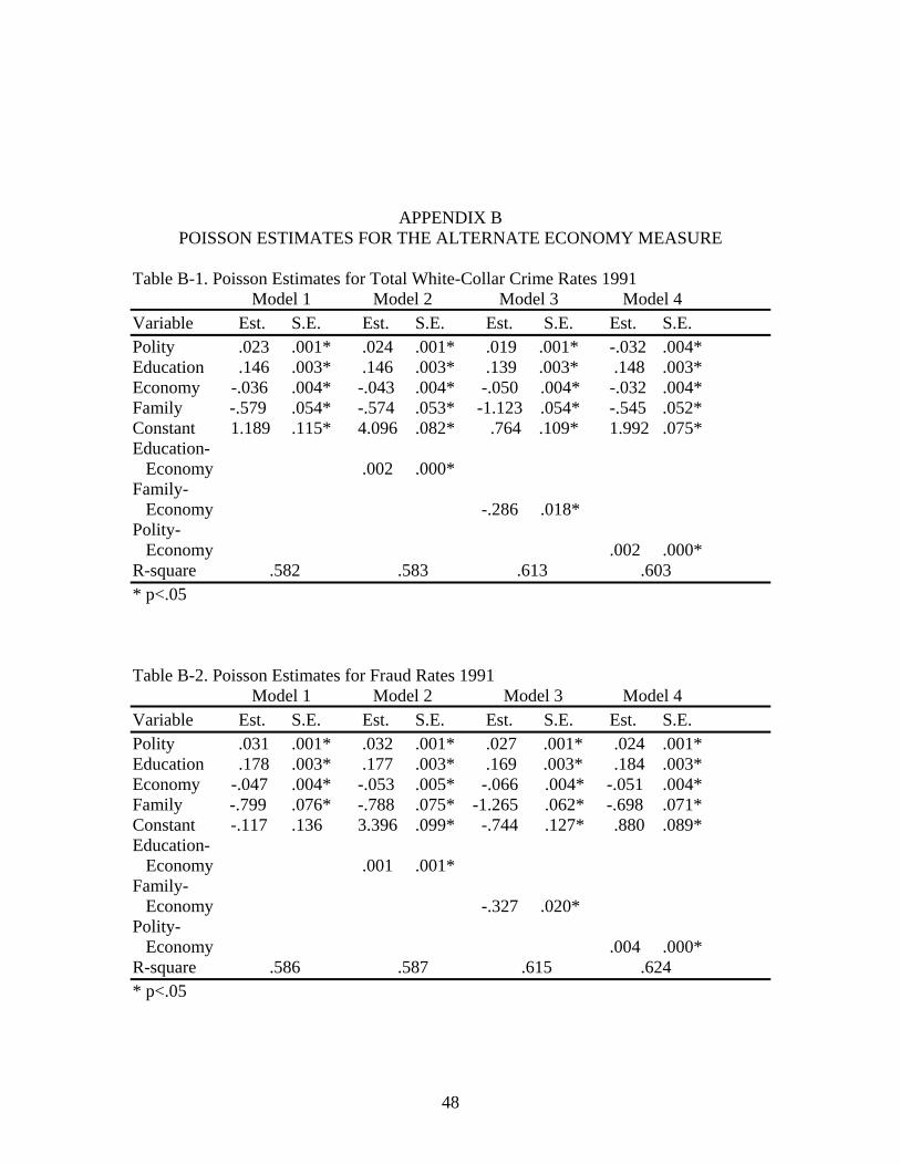
APPENDIX B POISSON ESTIMATES FOR THE ALTERNATE ECONOMY MEASURE

Table B-1. Poisson Estimates for Total White-Collar Crime Rates 1991 Model 1 Model 2 Model 3 Model 4 Variable Est. S.E. Est. S.E. Est. S.E. Est. S.E. Polity .023 .001* .024 .001* .019 .001* -.032 .004* Education .146 .003* .146 .003* .139 .003* .148 .003* Economy -.036 .004* -.043 .004* -.050 .004* -.032 .004* Family -.579 .054* -.574 .053* -1.123 .054* -.545 .052* Constant 1.189 .115* 4.096 .082* .764 .109* 1.992 .075* Education- Economy .002 .000* Family- Economy -.286 .018* Polity- Economy .002 .000* R-square .582 .583 .613 .603 * p<.05 Table B-2. Poisson Estimates for Fraud Rates 1991 Model 1 Model 2 Model 3 Model 4 Variable Est. S.E. Est. S.E. Est. S.E. Est. S.E. Polity .031 .001* .032 .001* .027 .001* .024 .001* Education .178 .003* .177 .003* .169 .003* .184 .003* Economy -.047 .004* -.053 .005* -.066 .004* -.051 .004* Family -.799 .076* -.788 .075* -1.265 .062* -.698 .071* Constant -.117 .136 3.396 .099* -.744 .127* .880 .089* Education- Economy .001 .001* Family- Economy -.327 .020* Polity- Economy .004 .000* R-square .586 .587 .615 .624 * p<.05

48

49

Table B-3. Poisson Estimates for Forgery/Counterfeiting Rates 1991 Model 1 Model 2 Model 3 Model 4 Variable Est. S.E. Est. S.E. Est. S.E. Est. S.E. Polity -.007 .003* -.004 .003 -.009 .003* -.015 .008* Education .045 .006* .045 .006* .041 .006* .045 .006* Economy -.011 .008 -.020 .008* -.015 .008 -.015 .008 Family -.293 .073* -.298 .073* -.775 .135* -.297 .073* Constant 3.318 .240* 4.050 .167* 3.214 .241* 2.747 .153* Education- Economy .003 .001* Family- Economy -.189 .046* Polity- Economy -.001 .000* R-square .233 .243 .254 .238 * p<.05 Table B-4. Poisson Estimates for Embezzlement Rates 1991 Model 1 Model 2 Model 3 Model 4 Variable Est. S.E. Est. S.E. Est. S.E. Est. S.E. Polity -.020 .006* -.022 .007* -.015 .007* -.012 .007 Education .028 .015 .027 .015 .033 .015* .033 .015* Economy .027 .020 .033 .023 .035 .020 -.001 .022 Family -.188 .167 -.184 .168 1.120 .347* -.205 .166 Constant 2.044 .608* 3.170 .411* 1.867 .594* 1.052 .399* Education- Economy -.001 .002 Family- Economy .549 .113* Polity- Economy -.002 .001* R-square .130 .131 .177 .146 * p<.05

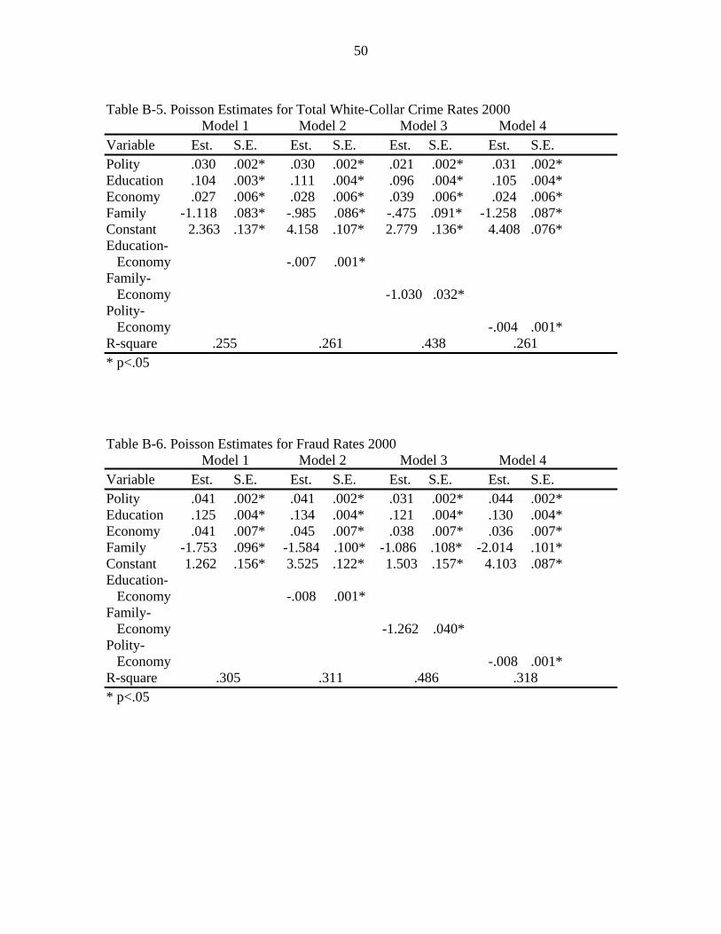
50

Table B-5. Poisson Estimates for Total White-Collar Crime Rates 2000 Model 1 Model 2 Model 3 Model 4 Variable Est. S.E. Est. S.E. Est. S.E. Est. S.E. Polity .030 .002* .030 .002* .021 .002* .031 .002* Education .104 .003* .111 .004* .096 .004* .105 .004* Economy .027 .006* .028 .006* .039 .006* .024 .006* Family -1.118 .083* -.985 .086* -.475 .091* -1.258 .087* Constant 2.363 .137* 4.158 .107* 2.779 .136* 4.408 .076* Education- Economy -.007 .001* Family- Economy -1.030 .032* Polity- Economy -.004 .001* R-square .255 .261 .438 .261 * p<.05 Table B-6. Poisson Estimates for Fraud Rates 2000 Model 1 Model 2 Model 3 Model 4 Variable Est. S.E. Est. S.E. Est. S.E. Est. S.E. Polity .041 .002* .041 .002* .031 .002* .044 .002* Education .125 .004* .134 .004* .121 .004* .130 .004* Economy .041 .007* .045 .007* .038 .007* .036 .007* Family -1.753 .096* -1.584 .100* -1.086 .108* -2.014 .101* Constant 1.262 .156* 3.525 .122* 1.503 .157* 4.103 .087* Education- Economy -.008 .001* Family- Economy -1.262 .040* Polity- Economy -.008 .001* R-square .305 .311 .486 .318 * p<.05

51

Table B-7. Poisson Estimates for Forgery/Counterfeiting Rates 2000 Model 1 Model 2 Model 3 Model 4 Variable Est. S.E. Est. S.E. Est. S.E. Est. S.E. Polity -.005 .004 -.005 .004 -.012 .004* -.005 .004 Education .016 .008* .015 .008 .006 .008 .016 .008* Economy -.002 .012 -.002 .012 .032 .013* -.002 .012 Family .600 .186* .577 .190* .998 .192* .604 .192* Constant 3.512 .307* 3.723 .241* 4.394 .300* 3.182 .169* Education- Economy .001 .002 Family- Economy -.687 .063* Polity- Economy .000 .002 R-square .025 .026 .155 .025 * p<.05 Table B-8. Poisson Estimates for Embezzlement Rates 2000 Model 1 Model 2 Model 3 Model 4 Variable Est. S.E. Est. S.E. Est. S.E. Est. S.E. Polity -.002 .010 -.001 .010 .000 .010 -.008 .010 Education .124 .017* .156 .018* .127 .017* .131 .017* Economy -.108 .028* -.099 .027* -.117 .029* -.108 .028* Family 2.077 .410* 2.564 .420* 1.966 .422* 2.956 .441* Constant .510 .714 .931 .575 .223 .695 -1.282 .405* Education- Economy -.030 .006* Family- Economy .127 .114 Polity- Economy .026 .004* R-square .114 .154 .115 .174 * p<.05

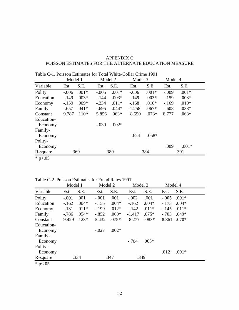
APPENDIX C POISSON ESTIMATES FOR THE ALTERNATE EDUCATION MEASURE

Table C-1. Poisson Estimates for Total White-Collar Crime 1991 Model 1 Model 2 Model 3 Model 4 Variable Est. S.E. Est. S.E. Est. S.E. Est. S.E. Polity -.006 .001* -.005 .001* -.006 .001* -.009 .001* Education -.149 .003* -.144 .003* -.149 .003* -.159 .003* Economy -.159 .009* -.234 .011* -.168 .010* -.169 .010* Family -.657 .041* -.695 .044* -1.258 .067* -.608 .038* Constant 9.787 .110* 5.856 .063* 8.550 .073* 8.777 .063* Education- Economy -.030 .002* Family- Economy -.624 .058* Polity- Economy .009 .001* R-square .369 .389 .384 .391 * p<.05 Table C-2. Poisson Estimates for Fraud Rates 1991 Model 1 Model 2 Model 3 Model 4 Variable Est. S.E. Est. S.E. Est. S.E. Est. S.E. Polity -.001 .001 -.001 .001 -.002 .001 -.005 .001* Education -.162 .004* -.155 .004* -.162 .004* -.173 .004* Economy -.131 .011* -.199 .012* -.142 .011* -.145 .011* Family -.786 .054* -.852 .060* -1.417 .075* -.703 .049* Constant 9.429 .123* 5.432 .075* 8.277 .083* 8.861 .070* Education- Economy -.027 .002* Family- Economy -.704 .065* Polity- Economy .012 .001* R-square .334 .347 .349 * p<.05

52

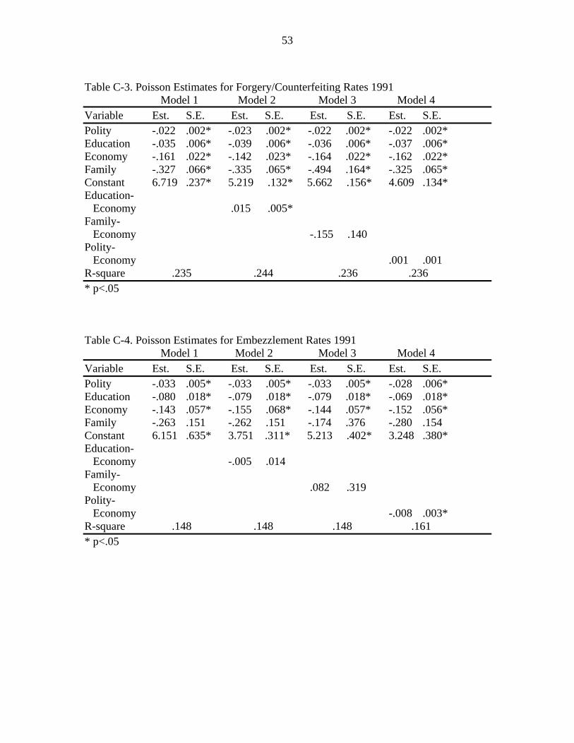
53

Table C-3. Poisson Estimates for Forgery/Counterfeiting Rates 1991 Model 1 Model 2 Model 3 Model 4 Variable Est. S.E. Est. S.E. Est. S.E. Est. S.E. Polity -.022 .002* -.023 .002* -.022 .002* -.022 .002* Education -.035 .006* -.039 .006* -.036 .006* -.037 .006* Economy -.161 .022* -.142 .023* -.164 .022* -.162 .022* Family -.327 .066* -.335 .065* -.494 .164* -.325 .065* Constant 6.719 .237* 5.219 .132* 5.662 .156* 4.609 .134* Education- Economy .015 .005* Family- Economy -.155 .140 Polity- Economy .001 .001 R-square .235 .244 .236 .236 * p<.05 Table C-4. Poisson Estimates for Embezzlement Rates 1991 Model 1 Model 2 Model 3 Model 4 Variable Est. S.E. Est. S.E. Est. S.E. Est. S.E. Polity -.033 .005* -.033 .005* -.033 .005* -.028 .006* Education -.080 .018* -.079 .018* -.079 .018* -.069 .018* Economy -.143 .057* -.155 .068* -.144 .057* -.152 .056* Family -.263 .151 -.262 .151 -.174 .376 -.280 .154 Constant 6.151 .635* 3.751 .311* 5.213 .402* 3.248 .380* Education- Economy -.005 .014 Family- Economy .082 .319 Polity- Economy -.008 .003* R-square .148 .148 .148 .161 * p<.05

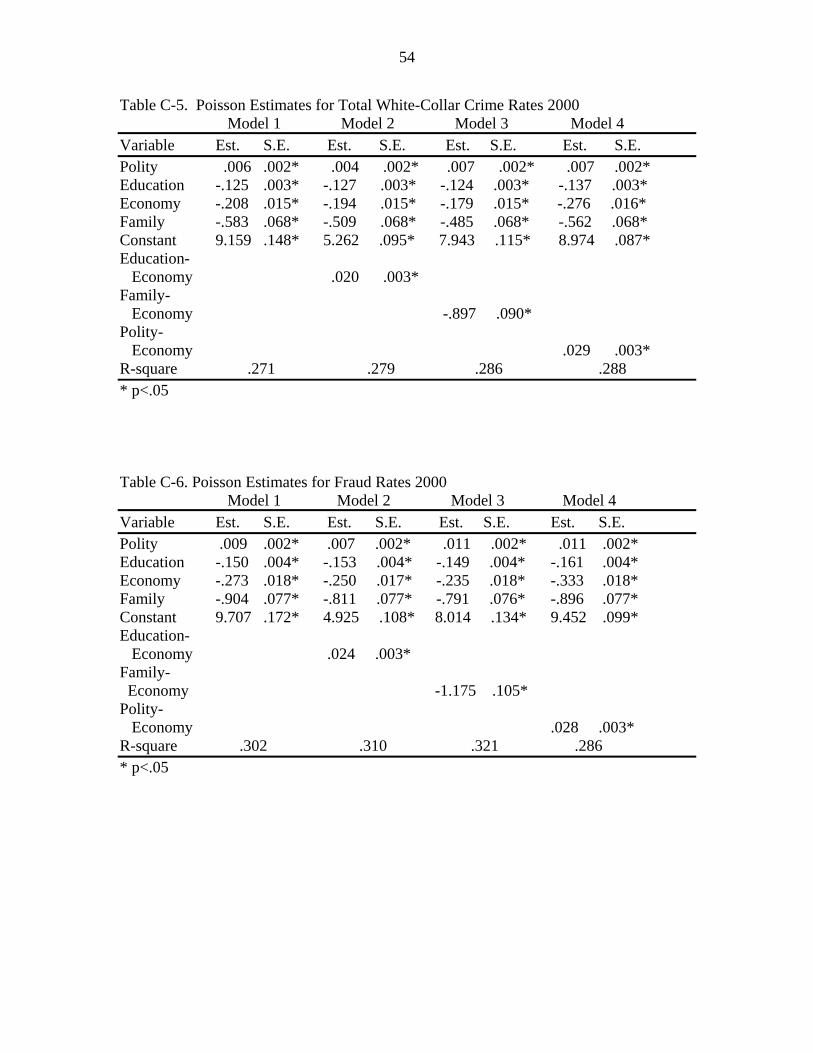
54

Table C-5. Poisson Estimates for Total White-Collar Crime Rates 2000 Model 1 Model 2 Model 3 Model 4 Variable Est. S.E. Est. S.E. Est. S.E. Est. S.E. Polity .006 .002* .004 .002* .007 .002* .007 .002* Education -.125 .003* -.127 .003* -.124 .003* -.137 .003* Economy -.208 .015* -.194 .015* -.179 .015* -.276 .016* Family -.583 .068* -.509 .068* -.485 .068* -.562 .068* Constant 9.159 .148* 5.262 .095* 7.943 .115* 8.974 .087* Education- Economy .020 .003* Family- Economy -.897 .090* Polity- Economy .029 .003* R-square .271 .279 .286 .288 * p<.05 Table C-6. Poisson Estimates for Fraud Rates 2000 Model 1 Model 2 Model 3 Model 4 Variable Est. S.E. Est. S.E. Est. S.E. Est. S.E. Polity .009 .002* .007 .002* .011 .002* .011 .002* Education -.150 .004* -.153 .004* -.149 .004* -.161 .004* Economy -.273 .018* -.250 .017* -.235 .018* -.333 .018* Family -.904 .077* -.811 .077* -.791 .076* -.896 .077* Constant 9.707 .172* 4.925 .108* 8.014 .134* 9.452 .099* Education- Economy .024 .003* Family- Economy -1.175 .105* Polity- Economy .028 .003* R-square .302 .310 .321 .286 * p<.05

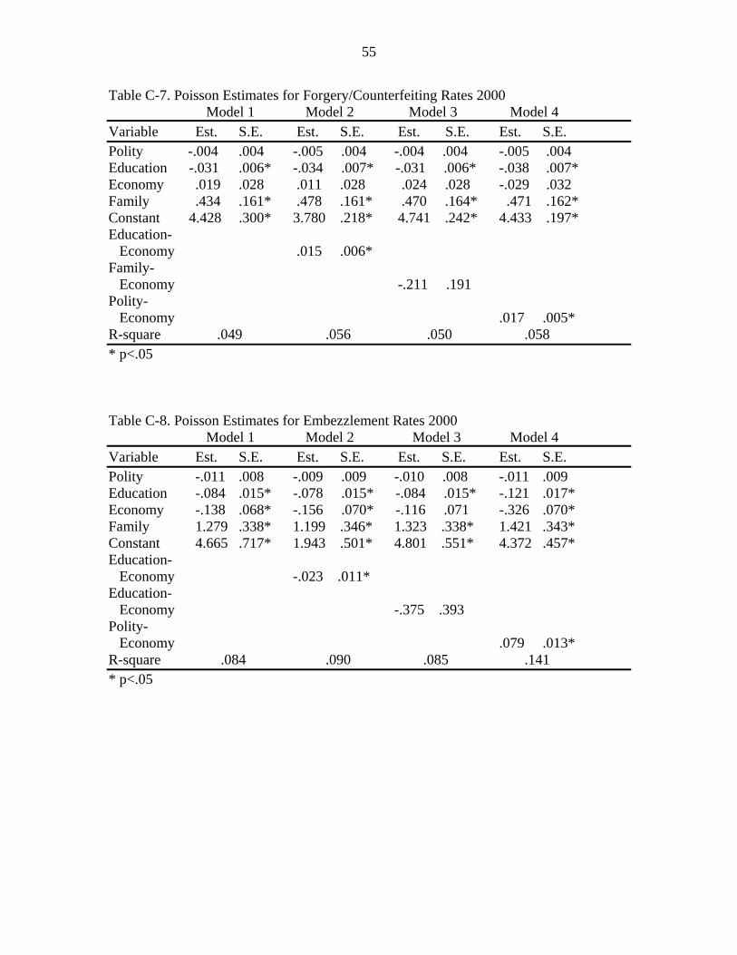
55

Table C-7. Poisson Estimates for Forgery/Counterfeiting Rates 2000 Model 1 Model 2 Model 3 Model 4 Variable Est. S.E. Est. S.E. Est. S.E. Est. S.E. Polity -.004 .004 -.005 .004 -.004 .004 -.005 .004 Education -.031 .006* -.034 .007* -.031 .006* -.038 .007* Economy .019 .028 .011 .028 .024 .028 -.029 .032 Family .434 .161* .478 .161* .470 .164* .471 .162* Constant 4.428 .300* 3.780 .218* 4.741 .242* 4.433 .197* Education- Economy .015 .006* Family- Economy -.211 .191 Polity- Economy .017 .005* R-square .049 .056 .050 .058 * p<.05 Table C-8. Poisson Estimates for Embezzlement Rates 2000 Model 1 Model 2 Model 3 Model 4 Variable Est. S.E. Est. S.E. Est. S.E. Est. S.E. Polity -.011 .008 -.009 .009 -.010 .008 -.011 .009 Education -.084 .015* -.078 .015* -.084 .015* -.121 .017* Economy -.138 .068* -.156 .070* -.116 .071 -.326 .070* Family 1.279 .338* 1.199 .346* 1.323 .338* 1.421 .343* Constant 4.665 .717* 1.943 .501* 4.801 .551* 4.372 .457* Education- Economy -.023 .011* Education- Economy -.375 .393 Polity- Economy .079 .013* R-square .084 .090 .085 .141 * p<.05

REFERENCES Bernburg, J.G. (2002). Anomie, social change and crime: A theoretical examination of institutional-anomie theory. British Journal of Criminology 42:729-742. Chamlin, M.B. and Cochran, J.K. (1995). Assessing Messner and Rosenfeld’s

institutional anomie theory: A partial test. Criminology 33:411-429. Chamlin, M.B. and Cochran, J.K. (1996). Reply to Jensen. Criminology 34:133-134.

Coleman, James W. (1994). Motivation and Opportunity: Understanding the Causes of

White-Collar Crime in White-Collar Crime: Classic and Contemporary Views. Third Edition. New York: The Free Press, 1995, pp.360-381.

Durkheim, Emile. (1951). Suicide, translated by John A. Spaulding and George Simpson,

edited by George Simpson. New York: The Free Press. Durkheim, Emile. (1965). The Division of Labor in Society, translated by George

Simpson. New York: The Free Press. Ermann, M.D. and Lundman,R. (2002). Corporate and Governmental Deviance. New

York: Oxford University Press. Geis, G., Meier, R.F., and Salinger, L.M. (1995). White-Collar Crime: Classic and

Contemporary Views. Third Edition. New York: The Free Press. Helmkamp, J, Ball, J. and Townsend, K. (1996). Definitional Dilema: Can and Should

There be a Universal Definition of White-Collar Crime? Morgantown, WV: National White-Collar Crime Center.

Hirschi, T. andGottfredson, M. (1989). The Significance of White-Collar Crime for a

General Theory of Crime. Criminology 27:359-371. Jensen, G.F. (1996). Comment on Chamlin and Cochran. Criminology 34:129-131. Meier, R. and Short, J. (1983). The Consequences of White-Collar Crime in White-Collar

Crime: Classic and Contemporary Views. Third Edition. New York: The Free Press, 1995, pp.80-104.

Merton, R.K. (1968). Social Theory and Social Structure. New York: The Free Press.

56

57

Messner, S.F. and Rosenfeld, R. (1994). Crime and the American Dream. Belmont, CA: Wadsworth.

Messner, S.F. and Rosenfeld, R. (1997). Political restraint of the market and levels of

criminal homicide: A cross-national application of institutional-anomie theory. Social Forces 75:393-416.

Messner, S.F. and Rosenfeld, R. (2001). Crime and the American Dream. Third Edition.

Belmont, CA: Wadsworth. Osgood, D.W. (2000). Poisson based regression analysis of aggregate crime rates.

Journal of Quantitative Criminology 16:21-44. Piquero, A. and Piquero, N. (1998). On testing institutional anomie theory with varying

specifications. Studies on Crime and Crime Prevention 7:61-84. Savolainen, J. (2000). Inequality, welfare state, and homicide: Further support for the

institutional anomie theory. Criminology 38:1021-1038. Sims, B. (1997). Crime, punishment, and the American Dream: Toward a Marxist

integration. Journal of Research in Crime and Delinquency 34:5-24. Steffensmeier, D. (1989). On the Causes of “White-Collar” Crime: An Assessment of

Hirschi and Gottfredson’s Claims. Criminology 27:345-358. Sutherland, E.H. (1940). White-collar criminality. American Sociological Review 5:1-12. Tapan, P.W. (1947). Who is the criminal? American Sociological Review 12:96-102. United States Bureau of Census. (1990). Statistical abstracts of the United States.

Washington, D.C.: Bureau of Census. United States Bureau of Census. (2000). Statistical abstracts of the United States.

Washington, D.C.: Bureau of Census. United States Department of Justice, Federal Bureau of Investigation. (1989). White

Collar Crime: A Report to the Public. Washington, D.C.: Government Printing Office.

United States Department of Justice, Federal Bureau of Investigation (1991). Uniform

Crime Reports. Washington, D.C.: Criminal Justice Information Services Division.

United States Department of Justice, Federal Bureau of Investigation (2000). Uniform Crime Reports. Washington, D.C.: Criminal Justice Information Services Division.

58

Vold, G., Bernard, T., and Snipes, J. (2002). Theoretical Criminology. New York: Oxford

University Press.

BIOGRAPHICAL SKETCH

Andrea Schoepfer received her Bachelor of Arts degree in Sociology from The

University of Florida in June, 2001. After taking one year off, she came back to The

University of Florida to earn her Master of Arts degree in Criminology in May, 2004.

She plans to continue her education working toward a PhD in Criminology from the

University of Florida.

59