experimental study of the quantum driven pendulum … study of the quantum driven pendulum and its...

PHYSICAL REVIEW A, VOLUME 64, 033407

Experimental study of the quantum driven pendulum and its classical analog in atom optics

W. K. Hensinger,1 A. G. Truscott,1 B. Upcroft,1 M. Hug,1 H. M. Wiseman,1,2 N. R. Heckenberg,1 and H. Rubinsztein-Dunlop1

1Centre for Laser Science, Department of Physics, The University of Queensland, Brisbane, Queensland 4072, Australia2School of Science, Griffith University, Nathan, Brisbane, Queensland 4111, Australia

~Received 30 August 2000; published 6 August 2001!

We present experimental results for the dynamics of cold atoms in a far detuned amplitude-modulatedoptical standing wave. Phase-space resonances constitute distinct peaks in the atomic momentum distributioncontaining up to 65% of all atoms resulting from a mixed quantum chaotic phase space. We characterize theatomic behavior in classical and quantum regimes and we present the applicable quantum and classical theory,which we have developed and refined. We show experimental proof that the size and the position of theresonances in phase space can be controlled by varying several parameters, such as the modulation frequency,the scaled well depth, the modulation amplitude, and the scaled Planck’s constant of the system. We have founda surprising stability against amplitude noise. We present methods to accurately control the momentum of anensemble of atoms using these phase-space resonances which could be used for efficient phase-space statepreparation.

DOI: 10.1103/PhysRevA.64.033407 PACS number~s!: 32.80.Pj, 05.45.Mt, 42.50.Vk

nmnri-tsrb

finlaeailaexaar

ifietdylaeopupbytirietun

-

ic-e

av

entlly

iesorp-of

b-

riedof

-edithaled

lleronsex-ges

tialsne-in

r totheesexi-

blethe

is

ely

ndon-

anics.nd

I. INTRODUCTION

The field of ‘‘quantum chaos’’ was born in 1917 wheAlbert Einstein tried to unravel which mechanical systecould be subjected to the Bohr-Sommerfeld-Epstein quazation rules@1#. He concluded that in the absence of invaant tori in phase space these quantization rules cannoused and that, moreover, this absence applies to mosttems. Chaos is associated with a rapid divergence of atrarily close points in phase space@2#. Strictly speaking therecan be no such thing as quantum chaos as an infinitelylevel of detail is needed to describe the trajectories of a csical chaotic system. In reality a system is bound by Heisberg’s uncertainty principle restricting the amount of detof position and momentum needed for classical chaos. Csical chaos can be described as the emergence of complon infinitely fine scales in classical phase space. In contrin quantum mechanics structure is smoothed away in anbelow the size of\ @2,3#.

During the years since the birth of quantum chaos, signcant amounts of theory have been created to give a bdescription of chaotic physical systems in a quantumnamical context. The key question is, what happens to csical chaos in the quantum world? One approach is to sgeneric features of quantum dynamics for a system whclassical description exhibits chaotic dynamics. One examof such features is dynamical localization, a quantum spression of classical diffusion, which was discoveredFishmanet al. @4# in numerical studies of the periodicallkicked quantum rotor. Conductance fluctuations in ballismicrostructures associated with complex electron trajectoconstitute another example of the occurrence of quanchaos @5#. Finally, molecular excitation experiments cashow interesting quantum features~e.g., Anderson localization, an effect related to dynamical localization! if the scaledPlanck’s constant is kept finite but exhibits chaotic dynamin the classical limit (\50) @6#. To gain a different perspective on the quantum nature of classical chaos some expments look at the manifestations of classical chaos in w

1050-2947/2001/64~3!/033407~15!/$20.00 64 0334

sti-

beys-i-

es-n-ls-ity

st,ea

-ter-s-eksele-

y

cs

m

s

ri-e

propagation. In these experiments the time-independwave equation, the Helmholtz equation, is mathematicaequivalent to the time-independent Schro¨dinger equation fora billiard system. In billiard-shaped cavities eigenfrequencand eigenfunctions can be measured by microwave abstion. In 1991 quantum scars, which are concentrationsprobability along periodic orbits, were experimentally oserved by Sridhar@7#. Experiments to study the quantumdynamics of classically chaotic systems have been carout on Rydberg atoms, measuring microwave ionizationhighly excited hydrogen atoms@8,9#. One result of these experiments is the recognition of different regimes determinby how well classical and quantum mechanics agree weach other. These regimes are characterized by the scmicrowave frequency given byV05n0V, wheren0 is theprincipal quantum number of the initial state andV the mi-crowave frequency.

It was first proposed by Graham, Schlautmann, and Zo@10# to use atom manipulation experiments to test predictiof quantum chaos. Cold atoms provide new grounds forperiments in quantum chaos which have some advantacompared to Rydberg atom experiments. First, the potenthat are used are extremely well approximated as odimensional potentials. In contrast, the potentials involvedthe Rydberg-atom ionization experiments are much hardeapproximate by one-dimensional potentials. At presentthree-dimensional quantum simulations needed for thhighly excited atoms are not feasible without severe appromations @9#. Second, in atom optics there is consideracontrol over the potentials. In the Rydberg-atom caseCoulomb potential dictates the dynamics and the systemcomplicated due to electron-electron interactions~the chaotictrajectory of the outer electron in a Rydberg atom can closapproach the shell of inner electrons!. In atom optics one cantailor the potentials to match the theoretical description aindeed achieve simple nonlinear potentials such as the nlinear pendulum which we consider in this study. We calso achieve a considerable variety of modulation dynamFinally, atom-optical systems are far less dissipative a

©2001 The American Physical Society07-1

linm

ia

kn

aot

t-li

ull-acdn

andind

cesiscin

od

zedlela-eceren

tomlleren

-sep

toit

tet

tuicnt

thealsoreso-ingtrolfordy-ofeffi-the

ve amill.

oldicalngof-

-

ing

auseen

l re-on-

it isand

W. K. HENSINGERet al. PHYSICAL REVIEW A 64 033407

noisy than Rydberg-atom experiments due to laser cooand the ability to operate far off resonance. Hence atooptical systems can be well approximated by Hamiltondynamics.

Moore et al. @11# and Ammannet al. @12# showed thatcold atoms can be used to simulate the quantum delta kicrotor ~Q-DKR!. Raizen’s group also reported the experimetal observation of dynamic localization in cold atoms@13#which is the quantum suppression of chaotic diffusion. It cbe roughly understood by considering that classical chapaths can interfere destructively. Decoherence will tendsuppress this quantum behavior and leads to classicaldynamics.

Our group has recently demonstrated the existencephase space resonances for the quantum driven pend~QDP! in cold atoms that we report on in this paper. Athough it is probably the first time that such phase-spresonances have been observed for the QDP, Raizen anworkers had previously observed momentum distributiothat are due to atoms being trapped in a first-order resonin the dynamics of cold atoms in a phase-modulated stanwave @14#. This particular first-order resonance corresponto the central elliptic fixed point at the origin of phase spaIn contrast we are investigating second-order resonancethe QDP, which are distinct features in the momentum dtribution of cold atoms traveling with a nonzero mean veloity on top of a background of atoms moving chaoticallyphase space.

Phase-space resonances have also been seen inphysical systems. For example, they have been reporteplasma physics. Sinclair, Hosea, and Sheffield@15# mapped atoroidal magnetic field in a stellarator using phase stabilielectrons. Islands of stability emerged in the phase-spacenamics of the electrons. In fluid flow experiments particmotion in the fluid was shown to have chaotic and reguphase-space regions@16#. In experiments on microwave ionization of Rydberg atoms strong classical resonance effin the final-bound-state quantum number distribution wfound by Bayfield and Sokol@17#. These peaks cannot bassociated with any quantum-mechanical resonance tration @9#.

Atom-optics experiments provide a good opportunityexamine the transition between classical and quantumchanics. Dyrting and co-workers@18# made a theoreticastudy of cold atoms which are subjected to a singfrequency amplitude-modulated standing wave. They pdicted quantum tunneling between phase-space resonafor this system. Hug and Milburn@19# showed that quantummechanical velocity predictions for second-order phaspace resonances disagree by up to 20% with classicaldictions in the quantum driven pendulum@20#.

We analyze in this study the phase-space resonanceswe found in the dynamics of the experimental realizationthe quantum driven pendulum and its classical analog wcold atoms and test theoretical predictions. The sysshows either classical or quantum behavior, depending onparameters chosen for the system. In the context of this swe mean by quantum behavior a situation where a classsimulation cannot predict some of the observed experime

03340

g-

n

ed-

nicoke

ofum

eco-sceg

s.

for--

therin

dy-

r

tse

si-

e-

--

ces

-re-

hatfhmhedyalal

features while a quantum simulation can. This constitutesimportance of the system for quantum chaos studies. Weanalyze here the observed second-order phase-spacenances in detail. We present experimental findings showhow they can be manipulated and how to momentum conthem. We give an overview of the resonance dynamicsdifferent parameter regimes to characterize the atomicnamics qualitatively and quantitatively. A surprising rangedynamics arises. Furthermore, we present methods forcient momentum phase-space state preparation utilizingquantum chaotic phase space of the QDP. This could havariety of applications in atom optics, for example beasplitters and atomic interferometry. Furthermore, we wshow introductory results on how noise affects the system

II. DESCRIPTION OF THE QUANTUM DRIVENPENDULUM AND ITS CLASSICAL ANALOG

Our QDP experiments have been carried out using crubidium atoms that are positioned in a far detuned optstanding wave. Modulation of the intensity of the standiwave leads to an effective Hamiltonian for the center-mass motion~as shown in the Appendix! given by

H5px

2

2m1

\Veff

4~122« sinvt !sin2~kx!, ~1!

where the effective Rabi frequency isVeff5V2/d, V5GAI /I sat is the resonant Rabi frequency,« is the modula-tion parameter,v is the modulation angular frequency,G isthe inverse spontaneous lifetime,d is the detuning of thestanding wave,t is the time, andpx the momentum component of the atom along the standing wave. HereI is thespatial mean of the intensity of the unmodulated standwave ~which is half of the peak intensity soV5GAI peak/2I sat) and I sat is the saturation intensity. Usingscaled variables@11# the Hamiltonian is given by

H5p2/212k~122« sint!sin2~q/2!, ~2!

whereH5(4k2/mv2)H, q52kx, p5(2k/mv)px and k isthe wave number. The driving amplitude is given by

k5v rVeff /v25

\k2Veff

2v2m, ~3!

wherev r5\k2/2m is the recoil frequency andt5tv is thescaled time variable. The commutator is given by

@p,q#5 i -k, ~4!

where the scaled Planck’s constant is-k58v r /v. This systemcan be seen to be equivalent to a driven pendulum, becthe Hamiltonian is equivalent to that of an amplitude-drivpendulum@18#.

The system exhibits classical and quantum-mechanicagimes determined by the value of the scaled Planck’s c

stant-k @10#. To understand the nature of the resonancesbest to estimate first when they can be treated classically

7-2

thn

enardth

t

ofemistycad

m

da

nilth

d

d

de-n

tiong

er

i-dto

n

tedn-

in

ht

alsee

dia-e-ifyebid

EXPERIMENTAL STUDY OF THE QUANTUM DRIVEN . . . PHYSICAL REVIEW A64 033407

when one has to use a full quantum simulation to predictdynamics of the system. The scaled Planck’s constant carewritten as

-k54\k2

vm54\

4p2

l2v54\p2S 1

l

2 S l

2TmD D 5

4\p2

2pI 05

h

I 0,

~5!

whereT is the modulation period,\ is Planck’s constant,l isthe wavelength, andI 0 is the action of a free particle over thdistancel/2 in the timeT. Our one-dimensional system cabe described in the corresponding two-dimensional phspace which is spanned by momentum and position coonates. The position coordinate axis is orientated alongstanding wave. The action of the system, multiplied by 2p,is given by the area in phase space, which is encircled by

trajectory of a particle.-k can be interpreted as the ratioPlanck’s constant to the action of a particle in the systdescribed. Now if the phase-space area of a resonancethe same order as\ we know that Heisenberg’s uncertainrelation forbids simulation of the dynamics using classitrajectories but it rather requires the atoms to be treate

wave packets. Thus-k will indicate in which regime the ex-periment is carried out. Therefore we know there is so

minimum order of magnitude of-k which must be exceedebefore we expect to see differences between quantumclassical dynamics on a given time scale.

Quantum effects can be observed only if the decohereis kept to a minimum. The magnitude of the detuning wdetermine the amount of decoherence introduced intosystem because the less the standing wave is detunemore incoherent transitions~e.g., spontaneous emission! willoccur. We now describe the full quantum dynamics, incluing spontaneous emission.

A. The quantum master equation

Quantum mechanically, the state of the system isscribed by a density operatorr. In order to describe spontaneous emission as well as the motion induced by the staing wave it is necessary to use a quantum master equaConsidering only motion in the direction of the standiwave, and working in the interaction picture, this is

r52i

\@H,r#1GL1r. ~6!

HereH is the Hamiltonian for the center-of-mass and intnal state of the atom, given by

H5px

2

2m2\ds†s2

\

2@V~x,t !s†1V†~x,t !s#. ~7!

Here V(x,t) is the position and time-dependent Rabfrequency operator for the atom in the standing wave andis the detuning of the standing wave. The atomic operaare defined in terms ofs5ua&^bu, whereua& and ub& corre-spond to ground and excited states, respectively.

03340

ebe

sei-e

he

on

las

e

nd

celethe

-

-

d-n.

-

rs

The superoperatorL describes the incoherent evolutiodue to the coupling to the vacuum field modes at rateG andis given by

L15E d2nW f~nW !D@eiknxxs#. ~8!

Here k is the wave number of the spontaneously emitlight, nW is a unit vector describing the direction of the spotaneously emitted photon, andf(nW ) is the dipole radiationdistribution for this direction

f~nW !53

8p S 12~dW •nW !2

dW •dWD , ~9!

wheredW is the atomic dipole vector. The superoperatorD isdefined for arbitrary operatorsA andB by

D@A#B[ABA†2~A†AB1BA†A!/2. ~10!

Only thex componentnx appears in the superoperatorEq. ~8! because we are only interested in motion in thexdirection. This is the direction of propagation of the ligbeams, so the dipole vector~which is parallel to the polar-ization vector of the light! is perpendicular to thex direction.This enables the integral in Eq.~8! to be simplified to

L15E du W~u!D@eikuxs#, ~11!

where

W~u!5H 3

8~11u2! for uuu<1

0 for uuu.1.

~12!

Note thatu can be interpreted as thex component of themomentum kick to the atom, in units of\k.

The evolution described by the master equation~6! is notobviously related to that generated by the Hamiltonian~1!.For a start, the real particle is an atom with two internstates whereas the ideal particle has no internal states. Tothe relation between the two models it is necessary to abatically eliminate the upper level of the atom. This procdure is outlined in the Appendix where we also quantsome of the approximations involved. It is valid only if thdetuningd is much greater than the maximum of the Rafrequency V(x,t). In the experiment the modulatestanding-wave Rabi frequency has the form

V~x,t !5VA122« sinvt sinkx, ~13!

which gives the master equation

r52i

\@H,r#1lL2r. ~14!

Here the Hamiltonian is

7-3

oh

nentic. Tnt

-di

siohes

etioe

iteahe7

mre

eby

.

m

kick

ua-

nvi-

bu-lof

.are

a-he


H5px

2

2m1

\Veff

4~122« sinvt !sin2~kx!, ~15!

which is the same as in Eq.~1!, with Veff5V2/d. The effec-tive damping rate isl5G(V/2d)2 and the superoperatorL2is

lL25lE du W~u!D @eikuxA122« sinvt sinkx#

~16!

5G

d

Veff

4~122« sinvt !E du W~u!D@eik(u11)x

2eik(u21)x#. ~17!

B. Simulation methods

To obtain reliable theoretical data we have utilized twdifferent methods to obtain our quantum simulations. Tdynamics are modeled using either the master equatioquantum trajectories. These methods are inherently differBoth have been tested and found to give essentially idenresults, strengthening the validity of the presented theoryallow a comparison with classical physics we also presemethod to obtain classical simulations. This will be of importance for future decoherence and quantum chaos stu

1. Simulations using the master equation

Since the Hamiltonian~15! is periodic inx, it would benatural to consider using the momentum states as a basisimulating the evolution. However, as the final express~17! for L2 indicates, spontaneous emission following tabsorption of a photon from the standing wave enabletransfer of momentum of any amount between22\k and12\k ~because the momentum kick is projected onto thxaxis!. This means that an exact one-dimensional simulaof the master equation would require a dense set of momtum states.

In practice, this dense set is not necessary as the inconditions have a finite momentum spread which will smout any fine structure. In fact, the initial conditions from texperimental setup have a momentum spread of order\kwhich means that features of order\k are not resolvable. Ittherefore makes sense to approximate the continuousmentum transfer due to spontaneous emission by discmomentum transfer in units of\k in order to take advantagof the symmetry of the Hamiltonian. This is achievedreplacingL2 by

L35~122« sinvt ! (u521,0,1

V~u!D @eik(u11)x2eik(u21)x#,

~18!

where V(u) is a discrete approximation toW(u). This issimilar to the approach of Ref.@21# but is more rigorous.

ApproximatingW(u) by V(u) is not a unique procedureHere we adopt the method of choosingV(u) such that thezeroth, first, and second moments agree. That is,

03340

eort.aloa

es.

forn

a

nn-

ialr

o-te

E W~u! du515V~21!1V~0!1V~1!, ~19!

E W~u!u du5052V~21!1V~1!, ~20!

E W~u!u2 du5 25 5V~21!1V~1!. ~21!

The first condition here is just thatV is normalized. Thesecond is thatV reproduces the correct mean momentukick ^Dp& in spontaneous emission~i.e., zero!. The third isthat V reproduces the correct mean squared momentum^(Dp)2&5(2/5)(\k)2. The three conditions imply

V~21!5 15 , V~0!5 3

5 , V~1!5 15 . ~22!

Under this approximation, we can write the master eqtion in the momentum basis as

r52i

\@H,r#1lL3r, ~23!

where

H51

2m (n

~p01\kn!2un&^nu

1\Veff

16~122« sinvt !~R21L222I !, ~24!

whereun& is the momentum stateup01\kn& ~wherep0 is anarbitrary momentum! and

L35 15 ~122« sinvt !$D@R22I #12D@R2L#1D@ I 2L2#%.

~25!

HereR is a unitary operator~corresponding toe2 ikx) whichraises the momentum by\k, andL ~corresponding toeikx)similarly lowers it by\k,

R5L215L†5(n

un11&^nu, ~26!

and I 5(nun&^nu.Since all of the operators in the master equation~23! can

be represented by matrices in theun& basis, it is a simplematter to solve the equation using a suitable numerical eronment such asMATLAB . The initial state matrixnur(0)un&is found by assuming a Gaussian initial momentum distrition of 1/e half width of 6.5\k which forms the diagonaelements ofr(0). To obtain smoother results a new setmomentum states is chosen, still spaced by\k, but shifted inmomentum by fractions of\k compared to the original setThe different density matrices are evolved and the resultscombined to gain a more accurate result.

2. Simulations using quantum trajectories

Without making the approximations of adiabatic elimintion of the upper level of the atom, and discretizing t

7-4

ac

toaktatb

arum

na

a

xstone

m

inica

x

r

tor

ay.nly

part

ep-f

cta-pec-

-y

othave

t ofdd to.rly

l astri-ex-e


spontaneous-emission recoil, it would be numerically intrtable to solve the initial master equation~6!. That is becauseof the size of the state matrix. However, it is possiblesimulate the evolution of that equation stochastically, by ting a large ensemble of quantum trajectories for the svector. This can be done as the number of elements ofstate vector is roughly equal to the square root of the numof elements of the state matrix.

The theory of quantum trajectories@22# shows that it ispossible to simulate incoherent transitions using Monte Cmethods@23#, so this was done to obtain our second quantmechanical simulations. A stochastic Schro¨dinger equationdeveloped for atom optics by Dum, Zoller, and Ritsch@24#and Mo” lmer, Castin, and Dalibard@25# is used to includeincoherent transitions.

Rather than simulate the exact dynamics of the origimaster equation~6! we follow Dyrting and Milburn@23# insimulating an approximate master equation. The approximmaster equation is similar to that of Eq.~14! in that the atomsees a potential. However, it is potentially a better appromation than that equation because we retain the excitedof the atomub&. We derive this approximate master equatias Eqs.~A7! and ~A8! in the Appendix, as a step along throute to deriving the master equation~14! used above. Themethod we use is related to, but uses different approxitions from, that of Dyrting and Milburn@23#.

In the quantum jump simulations the atom is alwaysstateub& or ua&, and the potential it sees depends on whstate it is in. Thus the atom has a quantum center-of-mstateuc& and an internal state which can be eithera or b butnot a superposition of both. The advantage of this appromation over the full master equation~6! is that it has a clearclassical analog, as will be discussed in Sec. II B 3.

In the scaled units of Eq.~2!, the stochastic equation fothe state vectoruc& is

duc&52i

-kdtKuc&1dN1~t!

3S A~122« sint!sin~q/2!

^cu@A~122« sint! sin~q/2!#2uc&21D uc&

1dN2~t!S exp~ ipq/-k!

A^cuc&21D uc&. ~27!

Here the non-Hermitian effective HamiltonianK depends onthe internal states5a,b of the atom

K5H p2/212k~122« sint!sin2~q/2!/n* for s5a

p2/222k~122« sint!sin2~q/2!/n for s5b~28!

with

n512iG

2d. ~29!

03340

-

-teheer

lo

l

te

i-ate

a-

hss

i-

The imaginary part ofn makesK non-Hermitian. The non-Hermitian part corresponds exactly to the anticommuta~the second term in the curly brackets! in Eqs. ~A7! and~A8!. It causes the modulus of the wave function to decThis is because the smooth evolution takes into account owhat happens when there are no jumps. The Hermitianof K corresponds exactly to the commutator~the first term inthe curly brackets! in Eqs.~A7! and~A8!. The Hermitian partof Ka ~for the ground state! also corresponds exactly to thHamiltonian which appears in the final equation of the Apendix, Eq.~A12!, which corresponds to the Hamiltonian oEq. ~14! in the experimentally relevant limit ofG!d (n'1).

The point process incrementsdN1(t) anddN2(t) are, inany infinitesimal time incrementdt, equal to either zero orone. The probabilities for the latter are equal to the expetion values of these stochastic processes and are, restively,

E@dN1#5h^cu~122« sint!sin2~q/2!uc&

^cuc&dt, ~30!

E@dN2#5~G/v!dt, ~31!

with

h5GV2

4vd2unu25

l

vunu2523Im

2k

-kn*. ~32!

The jumps~whendN151 or dN251) cause a discontinuous change inuc& given by Eq.~27!, and are accompanied ba change in the internal state of the atom as follows:

a →dN151

b absorption,

b →dN151

a stimulated emission, ~33!

b →dN251

a spontaneous emission.

It is the absence of the first jump process in the smoevolution which causes the decay in the modulus of the wfunction referred to above, and from Eq.~32! it is clear thatthe rate of these jumps is related to the non-Hermitian parthe effective HamiltonianK. When the modulus squaredrops below a preset random number, a jump is assumeoccur anddN1(t)51. This is explained in detail in Ref@24#. These jumps correspond to the third term in the cubrackets in Eqs.~A7! and ~A8!.

The second jump process~spontaneous emission! canonly occur when the atom is in the excited stateb. For aslong as the atom is in the excited state, the time untispontaneous emission has an exponential waiting time dibution with meanv/G, which is simple enough to calculatindependently of the wave function modulus. This is eplained in detail in Ref.@23#. These jumps correspond to thfirst term in Eqs.~A7! and ~A8!, proportional simply toG.

7-5

e

ofe

-

-

cereitiidt os-

e

-rm

f

isWe-

ror.of

onsiantion

e

in-od

ionys-l

eenlo-

ovenal

ory


When a spontaneous emission occurs, the atom receivrandom momentum kick represented byp in Eq. ~27!. It isgiven by @23#

p5-k sinf sinu, ~34!

where f and u are the Euler angles for the directionspontaneous emission relative to the atomic dipole mom~which is orthogonal to the direction of motionx). They aregenerated as follows:fP@0,2p) is a random angle with uniform distribution andu is given by

u5arccosF2 cosS arccos~2y21!14p

3 D G , ~35!

whereyP@0,1# is a random number with uniform distribution.

For the initial states we used squeezed minimum untainty wave packets with a momentum width which corsponds to the experimental spread in momentum of the incloud. The wave packets are initially equally spaced insone well of the standing wave. The smooth evolution parthe stochastic Schro¨dinger equation is solved numerically uing the split-operator method@26#. In this method the non-unitary Schro¨dinger equation

i -kd

dtuc&5Kuc& ~36!

has as a solution~for dt short enough to neglect the timdependence ofK) equal to

uc~t1dt!&5expS 2i~T1V!dt

-kD uc~t!&, ~37!

where T5p2/2 depends only onp and V5K2T dependsonly on q. Using the approximation

expS 2i ~T1V!dt

-kD 'exp~2 iTdt/2-k!exp~2 iVdt/-k!

3exp~2 iTdt/2-k!, ~38!

which is correct to order (dt)2; the evolution can be simulated very fast by using fast Fourier transforms to transfobetween the momentump and positionq bases. An adaptivetime stepsize method@27# is used to control the stepsize othe method. Once every§ steps the relative errorw is calcu-lated as

w5i uca&2ucb&i

i uc&i , ~39!

where

uca&5exp~2 iTdt/2-k!exp~2 iVdt/-k!exp~2 iTdt/2-k!uc&,~40!

ucb&5exp~2 iVdt/2-k!exp~2 iTdt/-k!exp~2 iVdt/2-k!uc&.

03340

s a

nt

r--alef

If the error lies above a specified tolerance the simulationrestarted§ steps before and the step size is decreased.have found§530 to work well. This method is used to prevent unphysical behavior due to a too large relative erFigure 1 shows a graphic representation of the methodquantum trajectories for our system.

3. Classical simulations

In the classical regime one can use Hamiltons’s equatito calculate the dynamics of the system. The Hamiltonevolution of a system preserves the Poisson bracket relabetween the position variableq and the momentum variablp @28#

$q~ t !,p~ t !%q,p51. ~41!

To prevent unphysical behavior when using a numericaltegration routine we used a symplectic integrator methwhich intrinsically preserves the Poisson bracket relat@29#. It was slightly changed to include time-dependent stems@33#. The Hamiltonian~which depends on the internastate of the atom! is given by

Hs5H p2/212k~122« sint!sin2~q/2! for s5a

p2/222k~122« sint!sin2~q/2! for s5b.~42!

This is identical to the non-Hermitian HamiltonianKs withn set to unity.

To gain a realistic model incoherent transitions have bincluded in the classical simulation. This can be done anagously to the quantum trajectory simulations described abusing a Monte Carlo simulation. The atom swaps interstatesa andb when a jump occurs as described in Eqs.~33!.The probabilities for the point process incrementsdN1 anddN2 are now given by

E@dN1#5h~122« cost!sin2~q/2!dt, ~43!

E@dN2#5~G/v!dt. ~44!

FIG. 1. Graphic representation of the quantum trajectmethod.

7-6

ren

man

ethna

totopt-otoin

ticisn

paossiorioumthailtuio

ono

rawg-

thg-hth

onthileinno

asthe-sm-in-ullythe

of

iths-

g toe of.es

rstMgh aedlec-

int-

ten-

ralhtuent

fibere

ro-


When a transition takes place the position of the atommains unchanged and the momentum is changed. Wheabsorption or stimulated emission takes place (dN251) mo-mentum of the atom changes by61 recoil. In case of aspontaneous emission the atom receives a random motum kick p calculated in exactly the same way as the qutum case.

4. Other theoretical considerations

The methods presented above lead to an atomic momtum distribution resulting from the interaction of atoms wia modulated optical standing wave which is turned off aon instantaneously. To obtain more accurate results we hadded into our numerical simulations the interaction duefinite turn-on and turn-off time of the standing wave duethe experimental restrictions when using an acousto-omodulator. The shape and length of the turn-on and turnwere measured using a 280 MHz bandwidth photodetecWe have also found that it is important to match the begning and end phase of the standing wave in our theoresimulations exactly with the experimental conditions. Thwas also accomplished using the photodetector mentioabove.

The experimentally measured data consists of atomicsition distributions after 10 ms ballistic expansion timedescribed in the section below. To obtain a theoretical ption distribution after 10 ms, we evolve the theoretical potion distribution after the standing-wave interaction f10 ms using a propagator method. The position distributafter 10 ms turns out to be very similar to the momentdistribution straight after the standing-wave interaction asfree evolution effectively transfers all the momentum fetures into the position distribution. Because of this we wsometimes refer to the experimental results as momendistributions, although they are, strictly speaking, positdistributions.

Finally one needs to consider the finite position widththe initial cloud, which will contribute to the final positiodistribution. Therefore we convolute the final theoretical psition distribution with the initial position distribution~be-fore the standing-wave interaction! to obtain our final theo-retical prediction.

III. EXPERIMENTAL SETUP

For our experiments a standard magneto-optic t~MOT! was used. The pressure in the vacuum chamberaround 1029 Torr. The magnetic field coils produced a manetic field gradient of 1021 T/m in an anti-Helmholtz con-figuration. The Earth’s magnetic field was zeroed usingHanle effect@30#. When applying a magnetic field the manitude of absorption of the laser beams changes sligwhen the laser is at resonance with the atomic vapor. Tcan be used to zero the magnetic field with high precisiAn injection-locking scheme was utilized to decreaselinewidth of the trapping diode laser down to 100 kHz, whallowing all the power of the laser to be used in the trappexperiment. Around 106 rubidium atoms were polarizatiogradient cooled for 10 ms. This brought the atoms down t

03340

-an

en--

n-

dvea

icffr.-al

ed

o-si--

n

e-lm

n

f

-

pas

e

lyis.

e

g

a

temperature of around 8mK. This corresponds to a 1/e mo-mentum spread of 13 recoil momenta. Then the MOT wturned off but the repumping beam was left on so thatatoms accumulated in theF53 ground state. After a repumping period of 500ms the optical standing wave waturned on. It was left on for a time corresponding to a nuber of periods of the modulation frequency. Both the begning and end phases of the modulation have to be carefchosen to ensure the visibility of the resonances. Afterstanding wave is switched off, the atoms undergo a periodballistic expansion~typically 10 ms for values of-k,0.1 andup to 16 ms for larger values of-k). Then an image of thecloud is taken using the freezing molasses method@11,31#. Inthis technique the optical molasses is turned on again wthe magnetic field still turned off and the resulting fluorecence is viewed with a 16 bit charge-coupled-device~CCD!camera. The CCD array of the camera was cooled, leadina quantum efficiency of around 80% and a rms read nois6.7 electrons. The experimental setup is shown in Fig. 2

A frequency stabilized titanium sapphire laser producup to 2.2 W of light at 780 nm with a linewidth of 1 MHzand a frequency drift of 50 MHz per hour. This beam is fipassed through an 80-MHz acousto-optic modulator (AO1as seen in Fig. 2! and then into a polarization-preservinsingle-mode optical fiber. The output beam goes througpolarizing beam-splitter cube and part of the light is fthrough a polarizer to a photodetector, which gives an etronic feedback signal to the AOM1 on the other end of thefiber. This reduces the standing-wave intensity noise, poing instability and polarization noise to less than 1%. AOM2modulates the amplitude of this beam and produces an insity modulation of the formI o(122« sinvt). High beamquality ~Gaussian profile! after the AOM2 is ensured bymonitoring the beam in the far field. To test the spectpurity of our modulated standing wave the modulated ligwave was observed on a fast photodetector and subseq

FIG. 2. Experimental setup used for our experiment.L1 , L2 arelenses used to couple the laser beam in and out of the opticalwhich is utilized to optimize the pointing stability and to improvthe quality of the laser beam. AOM1 stabilizes the light intensity.AOM2 produces the intensity modulation which is needed to pduce an amplitude-modulated standing wave.

7-7

r-en

its

-e.d.

e.eon


FIG. 3. The position of theresonances for loading and obsevation in phase space can be sein ~a!. To be able to resolve theresonances using a CCD camerais important that the resonancehave maximum velocity. Therefore they should be located on thmomentum axis for observationFor loading the resonances neeto be located on the position axisPart ~b! shows the initial distribu-tion of the atoms in phase spacThe pictures illustrates that thresonances need to be placedthe position axis for effectiveloading to occur.

o

ghdcaretheh

diurn

f tt

wim

,ipaeth

ninnn

teorepaadnde.

hecanute

reso-aosnack-

pro-o-

l re-ry

ksace

tofeseom

of

twothe

ical

uesnced

Fourier analysis of this signal indicated a spectral impurityabout one part in a thousand. The light after AOM2 is colli-mated to a 1/e width of 2.85 mm. The beam passes throuthe vacuum chamber and through the atomic cloud anretroreflected to form the one-dimensional periodic optipotential. The alignment of the retroreflection was measuto be good to approximately 0.02°. There is a variation ofscaled well depthk over the extent of the atomic cloud duto the Gaussian profile of our standing-wave beam. Tamounts to approximately 2%. The final maximum irraance of the standing wave in the region of the atomic clowas 36.461 W/cm2. The whole experiment is computecontrolled using the Labview programming environment aa general purpose interface bus~GPIB! interface.

IV. LOADING AND OBSERVATION OF RESONANCES

Poincare´ sections~stroboscopic phase-space maps! pro-vide an easy way to understand the classical dynamics osystem. Atoms that start in a phase-space resonance rotaphase space in time. Figure 3~a! shows the position of theresonances in phase space when they are loaded andthey are observed. The term ‘‘phase-space resonance’’plies that the resonances rotate with an angular velocitythat they have the same phase-space position after multof the modulation period. Therefore one cycle is definedone modulation period. Furthermore, it also implies that throtate with the same angular frequency as they would inunmodulated case in phase space~for a period 1 resonance!@18#. The resonances are loaded when they are located oposition axis in phase space. This is easy to understand sthen they overlap with the initial atomic distribution showin Fig. 3~b!. To observe the resonance experimentally ohas to wait for at least a quarter cycle~period 1 resonance!,so that the resonances turn 90° and are positioned onmomentum axis. When they are positioned on the momtum axis the standing wave is turned off. After a periodfree evolution the momentum distribution can now besolved experimentally by taking a picture of the atomic stial distribution. Exact velocity measurements can be mby taking pictures of the distribution after different times acalculating the distance they have moved during that tim

03340

f

islde

is-d

d

hee in

hen-

solessye

thece

e

hen-f--e

One needs to wait for approximately 4.25 cycles for tdynamics of the system to settle so that the resonancesbe observed. Chaotic motion needs some time to distribatoms, which are positioned in phase space between thenances initially, to other phase space regions where chpersists~sea of chaos, inside the region of bounded motio!.If this has occurred resonances can emerge from the bground of the chaotic region.

V. PHASE-SPACE CHARACTERIZATION UTILIZING THEMODULATION PARAMETER « AND THE DRIVING

AMPLITUDE k

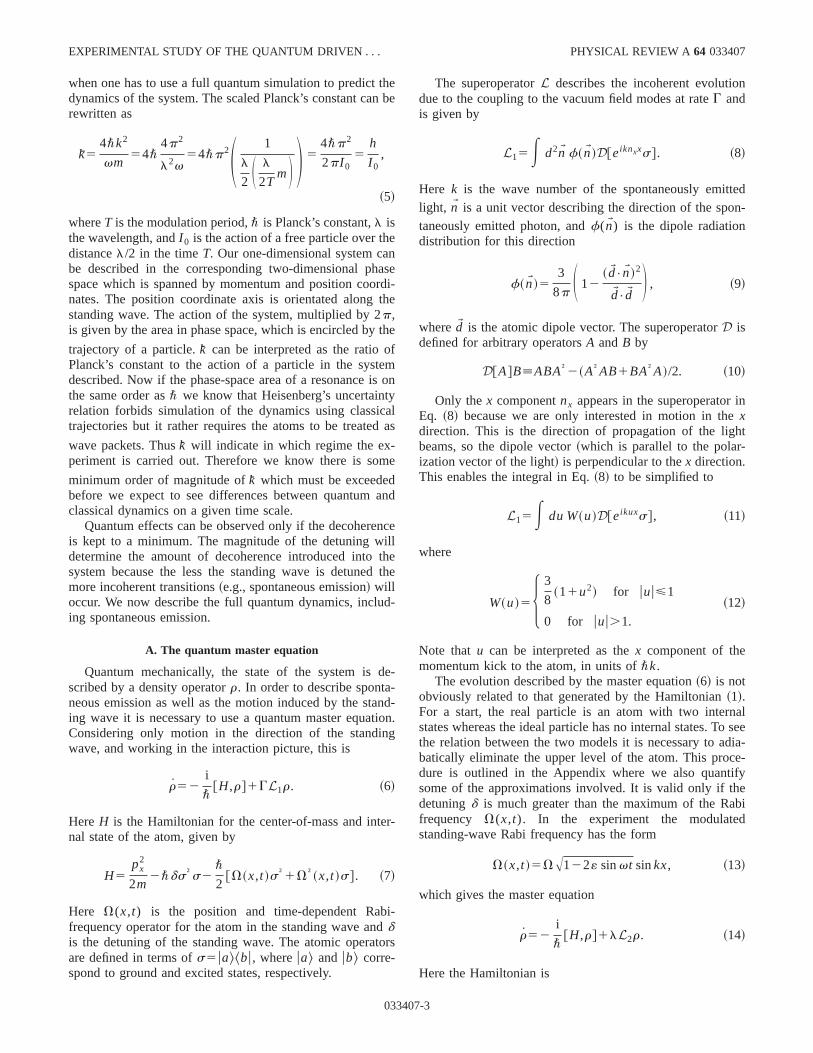
Using the techniques described above we are able tovide detailed experimental analysis of size, position, and mmentum of these resonances and compare experimentasults with the applicable theory. For this introductodiscussion we concentrate on experiments with-k50.1~modulation frequencyv/2p5300 kHz), being close to thequantum regime, when the modulation parameter« is variedand the scaled well depthk is held constant (k51.15). Theupper part of Figure 4 shows experimental results~solid line!as well as a quantum trajectory simulations~dotted line! forthe resulting atomic momentum distributions. Distinct peain the momentum distribution correspond to phase-spresonances. Below the experimental data, Poincare´ sectionsfor different values of the modulation parameter« illustratethe classical phase space. The Poincare´ sections are taken an11/4 periods of the modulation frequency. Two islandsstability can be seen, encircled by a sea of chaos. Thresult from second-order resonances, which bifurcate frthe origin atk51. The resonance width is proportional to«.However, the islands of stability break up for larger values« and therefore do not scale with«. It can be seen that thesize and the shape of the center resonance and thesecond-order resonances are strongly dependent onmodulation parameter. Figure 4~a! shows the unmodulatedcase. The region of bound motion is bound by the classseparatrix. The motion of all atoms is regular. In Fig. 4~b!two second-order resonances have emerged for«50.22. Theonset of chaotic motion can be seen. With increasing valof « the second-order resonances become more pronou

7-8

nter

t

otd

ohefinuula

sl

-b-

e-

t-

are

theer.

g

rr asa

la-or-mheos-ent.een

the

eterus

e-in

tiontemn-yoftheofchria-

dingnces

rethethendted.gherure-

mo-r

-


as can be seen in the experimental data and the quasimulations. The region of regular motion centered at zmomentum becomes smaller and eventually disappears insea of chaos as can be seen in Figs. 4~d!–4~f!. The smallregions of regular motion positioned close to the regionunbound motion~librations! do not rotate. This means thathey cannot be observed in the experiment as they neecross the position axis to be loaded as illustrated in Fig. 3~a!.

Due to the small initial momentum width, atoms are nloaded into the region of regular unbound motion. Nevertless, chaos leads to a homogeneous spread which is conby the region of regular unbound motion. The small shoders visible in both experimental data and quantum simtions result from this chaotic redistribution.

We have examined the phase space for different valuethe scaled driving amplitudek. Figure 5 shows experimenta

FIG. 4. The upper section shows the experimental atomicmentum distributions~solid line! together with a quantum simulation ~dotted line! using the trajectory method of Sec. II B 2 fodifferent values of the modulation amplitude«. The lower part il-lustrates the corresponding Poincare´ sections. The size of the resonances is strongly dependent on the modulation amplitude«.

03340

umohe

f

to

t-ed

l--

of

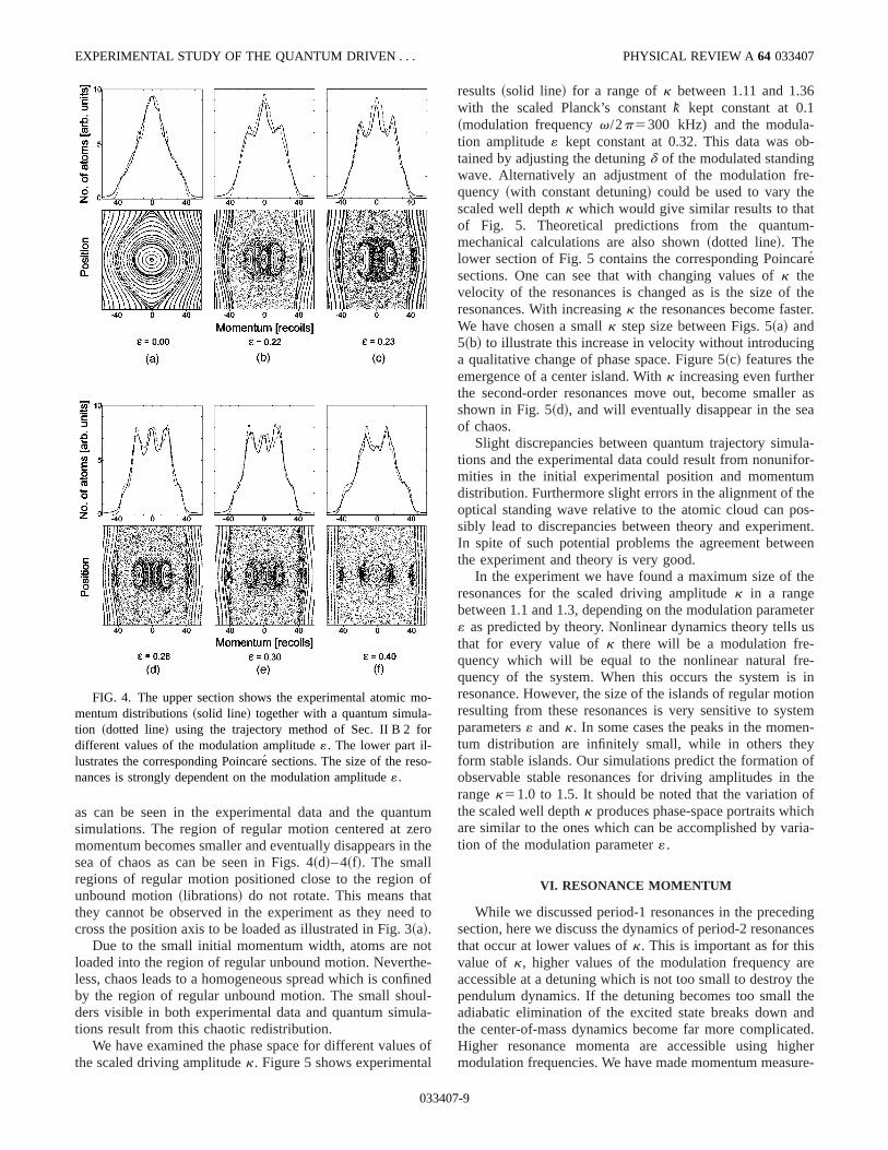
results~solid line! for a range ofk between 1.11 and 1.36with the scaled Planck’s constant-k kept constant at 0.1~modulation frequencyv/2p5300 kHz) and the modulation amplitude« kept constant at 0.32. This data was otained by adjusting the detuningd of the modulated standingwave. Alternatively an adjustment of the modulation frquency~with constant detuning! could be used to vary thescaled well depthk which would give similar results to thaof Fig. 5. Theoretical predictions from the quantummechanical calculations are also shown~dotted line!. Thelower section of Fig. 5 contains the corresponding Poinc´sections. One can see that with changing values ofk thevelocity of the resonances is changed as is the size ofresonances. With increasingk the resonances become fastWe have chosen a smallk step size between Figs. 5~a! and5~b! to illustrate this increase in velocity without introducina qualitative change of phase space. Figure 5~c! features theemergence of a center island. Withk increasing even furthethe second-order resonances move out, become smalleshown in Fig. 5~d!, and will eventually disappear in the seof chaos.

Slight discrepancies between quantum trajectory simutions and the experimental data could result from nonunifmities in the initial experimental position and momentudistribution. Furthermore slight errors in the alignment of toptical standing wave relative to the atomic cloud can psibly lead to discrepancies between theory and experimIn spite of such potential problems the agreement betwthe experiment and theory is very good.

In the experiment we have found a maximum size ofresonances for the scaled driving amplitudek in a rangebetween 1.1 and 1.3, depending on the modulation param« as predicted by theory. Nonlinear dynamics theory tellsthat for every value ofk there will be a modulation fre-quency which will be equal to the nonlinear natural frquency of the system. When this occurs the system isresonance. However, the size of the islands of regular moresulting from these resonances is very sensitive to sysparameters« andk. In some cases the peaks in the mometum distribution are infinitely small, while in others theform stable islands. Our simulations predict the formationobservable stable resonances for driving amplitudes inrangek51.0 to 1.5. It should be noted that the variationthe scaled well depthk produces phase-space portraits whiare similar to the ones which can be accomplished by vation of the modulation parameter«.

VI. RESONANCE MOMENTUM

While we discussed period-1 resonances in the precesection, here we discuss the dynamics of period-2 resonathat occur at lower values ofk. This is important as for thisvalue of k, higher values of the modulation frequency aaccessible at a detuning which is not too small to destroypendulum dynamics. If the detuning becomes too smalladiabatic elimination of the excited state breaks down athe center-of-mass dynamics become far more complicaHigher resonance momenta are accessible using himodulation frequencies. We have made momentum meas

-

7-9

e

arl


FIG. 5. Experimental data~solid line! and quantum trajectorysimulation ~dotted line! showingresonances as a function of thscaled driving amplitudek. Onecan see that the islands of regulmotion appear only for a smalrange ofk. The momentum of theresonances changes withk. Thecorresponding Poincare´ sectionsare shown below.

ee

ca

enc

deeo

aslsthhefr

d by

ntalri-bles.iqueo-ils

emre-e to

ch-

ments of the resonances for a range of modulation frequcies keepingk and« constant. The system can be describby the Hamiltonian given in Eq.~2!. As long ask and« arekept constant, the resonances will appear at the same smomentum. The measured momentumpx of the resonancesis proportional to the scaled momentump multiplied with themodulation frequencyv. Therefore, the momentum of thresonances should scale linearly with modulation freque

For different values of the modulation frequencyv, thedetuning was adjusted to obtain the same value of the molation parameterk. Then the momentum of the resonancwas measured using ballistic expansion. A graph of theperimental results is shown in Fig. 6. The resonance mmenta and their errors shown are obtained from a lesquares analysis of time-of-flight data. The error bars ainclude the momentum error resulting from the finite widof the resonances as well as slight asymmetries in tshape. There is a linear relation between the modulation

03340

n-d

led

y.

u-sx--t-o

ire-

quency and the momentum of the resonances as predictetheory.

In fact these results can be interpreted as the experimeproof for the mapping of several different physical expements into one unique theoretical case using scaled variaThe scaled quantum and classical theories produce a unresult for « and k kept constant, while the resonance mmentum can be varied experimentally from 0 to many recoby adjusting the modulation frequencyv while compensat-ing with the detuningd.

VII. EFFECTS OF SMALL NOISE AMPLITUDESON THE SYSTEM

Exploring the effects of noise on an atom-optical systis of importance as the mechanisms involved are closelylated to decoherence, which is an intense area of study duits importance for the development of new quantum te

f

-

FIG. 6. Momentum of theresonances for different values othe modulation frequencyv/2p.The modulation amplitudee andthe scaled well depthk are heldconstant. Results fore50.32 areshown. A linear fit is well withinthe error bars. This mechanismcould be used for effective velocity control of atoms.

7-10

tioic

a

tsvedueeth

ltd

eea

s isaree.ctsbe

atemi-to

tiontumeveuesorp-peri-ter-

the

or-d-

eadl to

en-ula-n-

nge

s aseseam-the

sod


nologies. Goetsch and Graham have undertaken a theorestudy where they analyzed the influence of spontaneemission on the dynamical localization in atommomentum-transfer experiments@34#. Experiments explor-ing the effects of noise and dissipation on dynamical locization were carried out by Klappaufet al. @35# and Ammannet al. @12,21#. We have studied how intensity noise affecthe stability and the loading of the resonances of the dripendulum. To implement this we added noise to the molated standing wave by adding a random number betwe21 and 1 multiplied by both the full modulation amplitudk and the noise factor between 0 and 1 to every point ofmodulation signal. This corresponds to adding white noisethe modulation signal. Figure 7 shows experimental resuFigure 7~a! shows the atomic distribution with no addenoise. In Fig. 7~b!, 10% amplitude noise~noise factor: 0.1!was added to the standing wave. Although the ratio betwthe height of the center resonance and the period 1 reson

FIG. 7. Amplitude noise is introduced to the system. The renances are remarkably stable. While there was no noise addepart~a!, 10% amplitude noise was added to obtain part~b!. The datawas obtained ate50.26.

03340

calus

l-

n-

n

etos.

nnce

changes slightly, the difference between the two casenearly negligible. It is remarkable that the resonancesfairly stable even with quite significant amounts of noisFurther experimental and theoretical studies of the effewhen stronger noise is introduced are under way and willreported in a future paper.

VIII. ATOMIC MOMENTUM STATE PREPARATION

For many experiments in atom optics momentum stpreparation is of significance. We have conducted prelinary experiments to achieve this goal. The final goal isefficiently prepare atomic wave packets at a certain posiin phase space with adjustable position and momenspread. Furthermore, it might also be desirable to achithis with a large-scaled Planck’s constant and at high valof detuning to prevent decoherence due to incoherent abstion and spontaneous-emission processes. We have exmentally shown that the momentum of resonances is demined by the value of the modulation frequency whenmodulation amplitude« and the modulation parameterk arekept constant as shown in Sec. VI. This provides the opptunity for rough momentum selection. Note that one disavantage of this method is the fact that the momentum sprof the atoms contained in the resonances is proportionathe modulation frequency.

Furthermore, the scaled theory predicts that the momtum of the resonances is slightly dependent on the modtion amplitude« as shown in Fig. 4. The resonance mometum is also strongly dependent on the scaled well depthk ascan be seen in Fig. 5. The disadvantage of trying to chathe resonance momentum by means of changing either« ork is that the amount of atoms contained in the resonancewell as the size change dramatically when changing thtwo parameters. Therefore changing either of these pareters does not represent an efficient solution to controlmomentum of an atomic ensemble.

-in

enben-a

on

FIG. 8. Resonances of the quantum-drivpendulum. Up to around 65% of the atoms canloaded into the resonances for effective mometum preparation. This data was obtained atmodulation parameter of 0.27 and a modulatifrequencyv/2p of 900 kHz.

7-11

hempa

isurod

bininctotioWo

thaltio.3

ehiioyc

thd

hae.

and

ofin

eters. Wepli-fre-

andro-bil-so-ibed

theedsethe

ces.hisre-vesave

his

ticef-pre-try,of a. Wean

th

e

2

so-ave.du-ula-of


We have found a far more efficient way to control tmomentum of an atomic ensemble while preserving atocoherence. Choosing the right parameters one can load u65% of all atoms into the resonances. Figure 8 showsexperimental atomic position distribution after 10-ms balltic expansion time. Here the two resonances were measto move with a momentum of 30.25 recoils. This methdoes not rely on changing any of the parametersk, -k, or «.The velocity of the resonances can be well controlledchanging the end phase of the modulation of the standwave. In this method we stop the modulation of the standwave at different times, not necessarily when the resonanare positioned on the momentum axis. This correspondsrotation of the resonances by up to 45° from the observaposition on the momentum axis as can be seen in Fig. 9.have achieved a velocity range of 35 recoils with this methwhich could be even further extended by increasingmodulation frequency. Figure 10 shows the experimentobtained velocities for different end phases of the modulasignal. The curve is approximately symmetric around 6cycles at which the resonances are positioned on the momtum axis. We have included a sinusoidal fit to show that tvelocity control mechanism can be explained by the rotatof the resonances in phase space. Note the two-cycle smetry of this experiment, due to the fact that the resonanwhich are utilized are period-2 resonances.

IX. CONCLUSION

Atom optics is an ideal experimental setting to explorequantum driven pendulum and its classical analog. Thenamics are best understood from a quantum chaotic pspace or the classical analog, depending at which valuthe scaled Planck’s constant-k the experiment is performed

FIG. 9. Rather than turning the standing wave off whenresonances are positioned on the momentum axis~position 3!, thestanding wave can be turned off slightly before or after that timThis corresponds to a rotation of the resonances by up to 45°~po-sitions 1,2,4,5! in phase space. Note the symmetry of positionsand 4, 1 and 5.

03340

icton

-ed

yggesane

delyn7n-

snm-es

ey-seof

In this paper we have presented experimental resultstheoretical techniques pertaining to this system.

We have given a thorough experimental investigationthe quantum chaotic phase space of the driven pendulumatom optics. We have characterized parts of the paramspace that determine the observed phase-space dynamicpresented experimental evidence for how the size and amtude of these resonances depend on the modulationquency, the scaled well depth, the modulation amplitudethe scaled Planck’s constant of the system. With the apppriate choice of parameters even the central island of staity can be eliminated while retaining the second-order renances. We have given experimental proof that the descrexperimental system used can be accurately modeled bytheory which we have provided here. We have developtwo experimental methods in which the momentum of theresonances can be controlled very accurately. One ofmethods allows us to fine tune the momentum of resonanExperimental evidence for the accuracy and efficiency of tmethod is given. In contrast to changing the modulation fquency as a means for momentum control this method leathe momentum width of the resonances unchanged. We hinvestigated the effect of small-noise amplitudes on tquantum chaotic system and found surprising stability.

In addition we have shown that the quantum chaomixed phase space provides a range of possibilities forfective quantum phase-space preparation. The resultssented here are likely to be useful for atom interferomeBragg scattering, and perhaps even the coherent splittingBose-Einstein condensate and other areas of atom opticshave shown that up to approximately 65% of all atoms c

e

. FIG. 10. Experimental data showing the momentum of the renances for different end phases of the modulated standing w6.37 cycles correspond to turning off the standing wave at a molation minimum. The data shown here were obtained at a modtion frequencyv/2p of 900 kHz and a modulation parameter0.27. A sinusoidal fit is within the error bars.

7-12

ve

exanlue

pere

tuic

kfues.Withtra

ila

tiongqu

tra

om

ed

lye

i-

thanthe

gy-


be loaded into the resonances, allowing efficient atomiclocity control.

Due to the control of the scaled Planck constant thisperiment provides an ideal environment for studies of qutum chaos and decoherence. Analyzing the driven penduin atom optics is an effective means to explore the bordland between quantum and classical physics as the exments illustrate that one needs to consider the wave natuatoms to accurately explain the atomic dynamics.

Further investigation is in progress addressing quanphenomena which can occur in this system, some of whare predicted by Dyrting, Milburn, and Holmes@18# andSanders and Milburn@32#.

ACKNOWLEDGMENTS

The corresponding author W.K.H. would like to thanGerard Milburn and Cathy Holmes for some very helpdiscussions as well as Howard Carmichael for some intering discussions concerning quantum trajectories. H.Mwould like to acknowledge enlightening discussions wPrahlad Warszawski. This work is supported by the Auslian Research Council.

APPENDIX: ADIABATIC ELIMINATION OF THEUPPER STATE

The adiabatic elimination technique we use here is simto that introduced by Graham, Schlautmann, and Zoller@10#for the same system, but we give a more complete derivaincluding justifications for the approximations made usithe parameters of the experiment. We also relate the etions to those of Dyrting and Milburn@23#, derived using adifferent technique, which are the basis for the quantumjectory simulations of this paper.

We can write the master equation for the two-level atin a light field as

r5GS Bsrs†21

2$s†s,r% D2

i

2@V~x,t !s†1sV†~x,t !,r#

2 id@s†s,r#2i

2\m@p2,r#, ~A1!

where for an arbitrary operatorR

BR5E d2nW f~nW !eiknxxRe2 iknxx. ~A2!

Explicitly using the internal state basisa,b we have

raa5GBrbb2i

2@V†~x,t !rba2rabV~x,t !#

2i

2\m@p2,raa#, ~A3!

03340

-

--mr-ri-of

mh

lt-.

-

r

n

a-

-

rab52G

2rab2

i

2@V†~x,t !rbb2raaV

†~x,t !#

1 idrab2i

2\m@p2,rab#, ~A4!

rbb52Grbb2i

2@V~x,t !rab2rbaV

†~x,t !#

2i

2\m@p2,rbb#. ~A5!

Now in the experimentuV(x,t)u&V'4.653109 s21,and d'7 GHz (d'443109 s21). Thus we are always inthe well-detuned regime whereV!d. As a result, most ofthe time the atom will be in the ground state withrbb;(V/d)2, as we will show. As long as we are not interestin evolution faster than the time scaleG21, we can then slaverab andrbb to raa . Specifically, we see from Eq.~A4! thatrab will quickly come to equilibrium~at rateG/2) with re-spect to the value ofraa , which evolves slowly. Settingrab50 thus gives

rab.i@raaV

†~x,t !2V†~x,t !rbb#

G22id. ~A6!

SinceV(x,t) is time dependent, this expression can onbe valid if the rate of decay,G/2, is much greater than thrate of variation of V(x,t). In the experimentG/2.193106 s21 while the angular modulation frequency is typcally an order of magnitude smaller. In deriving Eq.~A6! wehave also assumed that the kinetic energy is much less\d and\G and so can be ignored compared to them. Inexperimentd'443109 s21, G.3.83107 s21, and the re-coil frequency is 3.83103 s21. Since the 1/e momentumhalf-width is of order 7 recoil momenta, the kinetic enerdivided by \ is of order 105 s21. Thus the above assumptions are justified.

Substituting Eq.~A6! into Eq.~A5! and Eq.~A3! give thefollowing coupled equations:

raa5GBrbb11

G214d2$ id@V†~x,t !V~x,t !,raa#

2G$V†~x,t !V~x,t !,raa%/21GV†~x,t !rbbV~x,t !%

2i

2\m@p2,raa#, ~A7!

rbb52Grbb11

G214d2$2 id@V~x,t !V†~x,t !,rbb#

2G$V~x,t !V†~x,t !,rbb%/21GV~x,t !raaV†~x,t !%

2i

2\m@p2,rbb#. ~A8!

7-13

tu

lly

te

iv

-di

angate

i-a-la-final

-


These are the equations which are simulated by the quantrajectories in Sec. II B 2.

We can simplify the system still further by adiabatica

eliminating the upper staterbb , by settingrbb50. This re-quires that the damping rateG be much greater than the raof variation ofV(x,t) and the kinetic energy divided by\.These are the same approximations as used above in derEq. ~A6!. Strictly, this technique also requires thatG bemuch greater thanV2/d, which is not satisfied for our system. It can be shown that a more rigorous approach to a

the

sfyhrmi

los

ing

e

s

e

03340

m

ing

a-

batic elimination@36# removes this requirement, and givesslightly different result in the end. This is based on moviinto the interaction picture with respect to the ground-stpotentialH05(\/4d)V(x,t)V†(x,t) ~which results from theadiabatic elimination! before beginning the adiabatic elimnation. It does not yield the above Dyrting-Milburn equtions which are the basis for our quantum trajectory simutions. For this reason, and because the correction to ourmaster equation is small, we will continue to follow the simpler procedure we have used so far.

Slavingrbb to raa by settingrbb50 gives

rbb1$V~x,t !V†~x,t !,rbb%/21 i ~d/G!@V~x,t !V†~x,t !,rbb#

G214d2.

V~x,t !raaV†~x,t !

G214d2. ~A9!

tion

anisrm

The first correction term on the left-hand side~LHS! ~theanticommutator! scales likeV2/4d2, which is, as we haveshown above, negligible. The second correction term onLHS ~the commutator! cannot be removed so simply, sinc~as noted above! the experimental parameters do not satiG@V2/d. In the more sophisticated treatment of making tadiabatic approximation in an interaction picture, this tedoes not appear. Knowing this, we can justify droppinghere. Thus we arrive at the simple expression

rbb.V†~x,t !raaV~x,t !

G214d2, ~A10!

which scales as (V/d)2 as claimed.The reduced density operator for the center-of-mass a

is given by the partial trace over the internal atomic state

rcom5Trintr5raa1rbb ~A11!

e

e

t

ne:

Denoting rcom simply asr, the above scaling implies thar.raa . Using this, and substituting the above expressfor rbb into Eq. ~A3! gives finally

r5G

G214d2 S BV†~x,t !rV~x,t !21

2$V~x,t !V†~x,t !,r% D

2 id

G214d2@V~x,t !V†~x,t !,r#2

i

2\m@p2,r#. ~A12!

For d@G this is identical to Eq.~14!. The more sophisticatedadiabatic elimination would produce an extra Hamiltoniterm scaling asV4/d3. For the experimental parameters, this only about 1% as large as the dominant Hamiltonian tescaling asV2/d, and can thus be safely ignored.

and

en,

nd

.A.ys.

In-

oc.

@1# A. Einstein, Verh. Dtsch. Phys. Ges.19, 82 ~1917!.@2# M.V. Berry. Proc. R. Soc. London, Ser. A413, 183 ~1987!.@3# K. Nakamura,Quantum versus Chaos. Questions Emerg

from Mesoscopic Cosmos~Kluwer Academic, Dordrecht,1997!.

@4# S. Fishman, D.R. Grempel, and R.E. Prange, Phys. Rev. L49, 509 ~1982!.

@5# C.M. Marcus, A.J. Rimberg, R.M. Westervelt, P.F. Hopkinand A.C. Gossard, Phys. Rev. Lett.69, 506 ~1992!.

@6# R. Blumel, S. Fishman, and U. Smilansky, J. Chem. Phys.84,2604 ~1986!.

@7# S. Sridhar. Phys. Rev. Lett.67, 785 ~1991!.@8# J.E. Bayfield and P.M. Koch, Phys. Rev. Lett.33, 258 ~1974!.@9# R.V. Jensen, S.M. Susskind, and M.M. Sanders, Phys. R

201, 1 ~1991!.@10# R. Graham, M. Schlautmann, and P. Zoller, Phys. Rev. A45,

R19 ~1992!.

tt.

,

p.

@11# F.L. Moore, J.C. Robinson, C.F. Bharucha, B. Sundaram,M.G. Raizen, Phys. Rev. Lett.75, 4598~1995!.

@12# H. Ammann, R. Gray, I. Shvarchuck, and N. ChristensPhys. Rev. Lett.80, 4111~1998!.

@13# F. L. Moore, J. C. Robinson, C. Bharucha, P. E. Williams, aM. G. Raizen, Phys. Rev. Lett.73, 2974~1994!.

@14# J.C. Robinson, C. Bharucha, F.L. Moore, R. Jahnke, GGeorgakis, Q. Niu, M.G. Raizen, and Bala Sundaram, PhRev. Lett.74, 3963~1995!.

@15# R.M. Sinclair, J.C. Hosea, and G.V. Sheffield, Rev. Sci.strum.41, 1552~1970!.

@16# J. Chaiken, R. Chevray, M. Tabor, and Q.M. Tan, Proc. R. SLondon, Ser. A408, 165 ~1986!.

@17# J.E. Bayfield and David S. Sokol, Phys. Rev. Lett.61, 2007~1988!.

@18# S. Dyrting, G.J. Milburn, and C.A. Holmes, Phys. Rev. E48,969 ~1993!.

7-14

J.

m

ys.

H.

94.

n,


@19# M. Hug and G.J. Milburn, Phys. Rev. A63, 023413~2001!.@20# W. Chen, S. Dyrting, G.J. Milburn, Aust. J. Phys.49, 777

~1996!.@21# G.H. Ball, K.M.D. Vant, H. Ammann, and N.L. Christensen,

Opt. B: Quantum Semiclassical Opt.1, 357 ~1999!.@22# H.J. Charmichael,An Open Systems Approach to Quantu

Optics ~Springer-Verlag, Berlin, 1993!.@23# S. Dyrting and G.J. Milburn, Phys. Rev. A51, 3136~1995!.@24# R. Dum, P. Zoller, and H. Ritch, Phys. Rev. A45, 4879~1992!.@25# K. Mo” lmer, Y. Castin and J. Dalibard, J. Opt. Soc. Am. B10,

524 ~1993!.@26# M.D. Feit, J.A. Fleck, Jr., and A. Steiger, J. Comput. Phys.47,

412 ~1982!.@27# S.M. Tan and D.F. Walls, J. Phys. II4, 1897~1994!.

03340

@28# R.D. Ruth, IEEE Trans. Nucl. Sci.NS-30, 2669~1983!.@29# E. Forest and M. Berz, inLie Methods in Optics II, edited by

K.B. Wolf ~Springer-Verlag, Berlin, 1989!, p. 47.@30# J. Dupont-Roc, S. Haroche, and C. Cohen-Tannoudji, Ph

Lett. A 28A, 638 ~1969!.@31# A.G. Truscott, D. Baleva, N.R. Heckenberg, and

Rubinsztein-Dunlop, Opt. Commun.145, 81 ~1998!.@32# B.C. Sanders and G.J. Milburn, Z. Phys. B:77, 497 ~1989!.@33# S. Dyrting, Ph.D. thesis, The University of Queensland, 19@34# P. Goetsch and R. Graham, Phys. Rev. A54, 5345~1996!.@35# B. G. Klappauf, W. H. Oskay, D. A. Steck, and M. G. Raize

Phys. Rev. Lett.81, 1203~1998!.@36# P. Warszawksi and H.M. Wiseman, Phys. Rev. A63, 013803

~2000!.

7-15

experimental study of the quantum driven pendulum … study of the quantum driven pendulum and its...

Documents