experimental study of router buffer sizing - high performance
TRANSCRIPT

Experimental Study of Router Buffer Sizing� y
Neda BeheshtiDepartment of ElectricalEngineering, Stanford
University, Stanford, CA, [email protected]
Yashar GanjaliDepartment of Computer
Science, University of Toronto,Toronto, ON, Canada
Monia GhobadiDepartment of Computer
Science, University of Toronto,Toronto, ON, Canada
Nick McKeownDepartment of ElectricalEngineering, Stanford
University, Stanford, CA, [email protected]
Geoff SalmonDepartment of Computer
Science, University of Toronto,Toronto, ON, Canada
ABSTRACT
During the past four years, several papers have proposedrules for sizing buffers in Internet core routers. Appenzelleret al. suggest that a link needs a buffer of size O(C=
pN),
where C is the capacity of the link, and N is the number offlows sharing the link. If correct, buffers could be reducedby 99% in a typical backbone router today without loss inthroughput. Enachecsu et al., and Raina et al. suggest thatbuffers can be reduced even further to 20-50 packets if weare willing to sacrifice a fraction of link capacities, and ifthere is a large ratio between the speed of core and accesslinks. If correct, this is a five orders of magnitude reduc-tion in buffer sizes. Each proposal is based on theoreticalanalysis and validated using simulations. Given the poten-tial benefits (and the risk of getting it wrong!) it is worthasking if these results hold in real operational networks. Inthis paper, we report buffer-sizing experiments performedon real networks - either laboratory networks with commer-cial routers as well as customized switching and monitoringequipment (UW Madison, Sprint ATL, and University ofToronto), or operational backbone networks (Level 3 Com-munications backbone network, Internet2, and Stanford).The good news: Subject to the limited scenarios we cancreate, the buffer sizing results appear to hold. While weare confident that the O(C=
pN) will hold quite generally
for backbone routers, the 20-50 packet rule should be ap-
�This work was supported under DARPA/MTO DOD-N award no. W911NF-04-0001/KK4118 (LASORPROJECT), and the Buffer Sizing Grant no. W911NF-05-1-0224 and W911NF-07-1-0024. University of Toronto’swork was supported by NSERC Discovery, NSERC RTI aswell as a grant from Cisco Systems.yThe experiments’ data is available online at:http://sysweb.cs.toronto.edu/bsizing/
Permission to make digital or hard copies of all or part of this work forpersonal or classroom use is granted without fee provided that copies arenot made or distributed for profit or commercial advantage and that copiesbear this notice and the full citation on the first page. To copy otherwise, torepublish, to post on servers or to redistribute to lists, requires prior specificpermission and/or a fee.IMC’08, October 20–22, 2008, Vouliagmeni, Greece.Copyright 2008 ACM 978-1-60558-334-1/08/10 ...$5.00.
plied with extra caution to ensure that network componentssatisfy the underlying assumptions.
Categories and Subject Descriptors
C.2 [Computer-Communication Networks]: Internet-working
General Terms
Experimentation, Measurement, Performance
Keywords
NetFPGA, Network Test-beds, Router Buffer Size, TCP
1. MOTIVATION AND INTRODUCTIONMost routers in the backbone of the Internet have a band-
width delay product worth of buffering for each link; i.e.B = 2T � C, where C is the bottleneck link capacity, and2T is the effective two-way propagation delay (RTT) of TCPflows through the core router [16, 17, 27]. This value is rec-ommended by Internet RFCs [6], architectural guidelines,and network operators.
On the other hand, several recent papers propose con-siderably reducing the buffers in backbone routers [4, 9, 23].For example, Appenzeller et al. [4] propose that the buffers
can be reduced to 2T � C=pN , where N is the number
of long-lived flows sharing the link. Throughout the paperwe will refer to this as the small buffer model. The basicidea follows from the observation that the buffer size is, inpart, determined by the sawtooth window size process ofthe TCP flows. The bigger the sawtooth, the bigger thebuffers need to be in order to guarantee 100% throughput.As the number of flows increases, variations in the aggregatewindow size process (the sum of all the congestion windowsize processes for each flow) decrease, following the centrallimit theorem. The result relies on several assumptions: (1)that flows are sufficiently independent of each other to bedesynchronized, (2) that the buffer size is dominated by thelong-lived flows, and, perhaps most importantly, (3) thatthere are no other significant unmodeled reasons for buffer-ing more packets. If the result is correct, then a backbonelink carrying 10,000 long-lived flows could have its buffersize reduced by a factor of 100 without loss in throughput.
If, though, the result is wrong, then the consequences ofreducing the buffer sizes in a router, or in an operationalcommercial network, could be quite severe. The problem is,how to decide if the result is correct, without trying it inan operational network? But who would reduce buffers inan operational network, and risk losing customers’ traffic,before knowing if the result is correct?
It is, therefore, not surprising that, apart from the re-sults we present here, we are not aware of any backbonecommercial network in which the buffers have been reducedto anywhere close to 2T � C=
pN . So the first goal of our
work is to experiment with small buffers in laboratory andoperational networks.
More recently, Enachescu et al. [9] and Raina et al. [23]propose reducing buffers much further to O(logW ) pack-ets in backbone routers, where W is the congestion windowsize. This translates to a few dozen packets for present-daywindow sizes [9]. We will refer to this as the tiny buffermodel. In [9], the authors reach their conclusion by consid-ering the tradeoff between reducing buffers and losing somethroughput – assumed to be 10-20%. In other words, whencongested, links behave as if they run at 80-90% of theirnominal rates. This could be an interesting assumption innetworks with abundant link capacity, or in future opticalnetworks where link capacity might be cheaper than buffers.The results depend on the network traffic being non-bursty,which they propose can happen in two ways: (1) if the corelinks run much faster than the access links (which they dotoday), then the packets from a source are spread out andbursts are broken, or (2) TCP sources are changed so as topace the delivery of packets. If the results are correct, andrelevant, then a backbone link could reduce its buffers byfive orders of magnitude.
Again, it is difficult to validate these results in an oper-ational network, and we are not aware of any other com-prehensive laboratory or network experiments to test theO(logW ) results. So it is the second goal of our work toexperiment with tiny buffers in laboratory and operationalnetworks.
In the remainder of this paper we describe a number of lab-oratory and network experiments performed between 2003and 2008. The laboratory experiments were performed inthe WAIL laboratory at University of Wisconsin Madison,in the Sprint Advanced Technology Laboratory, and in Uni-versity of Toronto’s Advanced Packet Switch and Network-ing Laboratory. Experiments were also performed on thefollowing operational networks: Level 3 Communications’operational backbone network, Internet2 and a the Stan-ford University dormitory network. We should make clearthat our results are necessarily limited; while a laboratorynetwork can use commercial backbone routers and accurateTCP sources, it is not the same as a real operational back-bone network with millions of real users. On the other hand,experiments on an operational network are inevitably lim-ited by the ability to control and observe the experiments.Commercial routers do not offer accurate ways to set thebuffer size and do not collect real-time data on the occu-pancy of their queues. Real network experiments are not re-peatable for different buffer sizes, making apples-with-applescomparisons difficult.
In laboratory experiments, we generate live TCP traffic(ftp, telnet, or http) using a cluster of PCs or commercialtraffic generators. We measure the performance from either
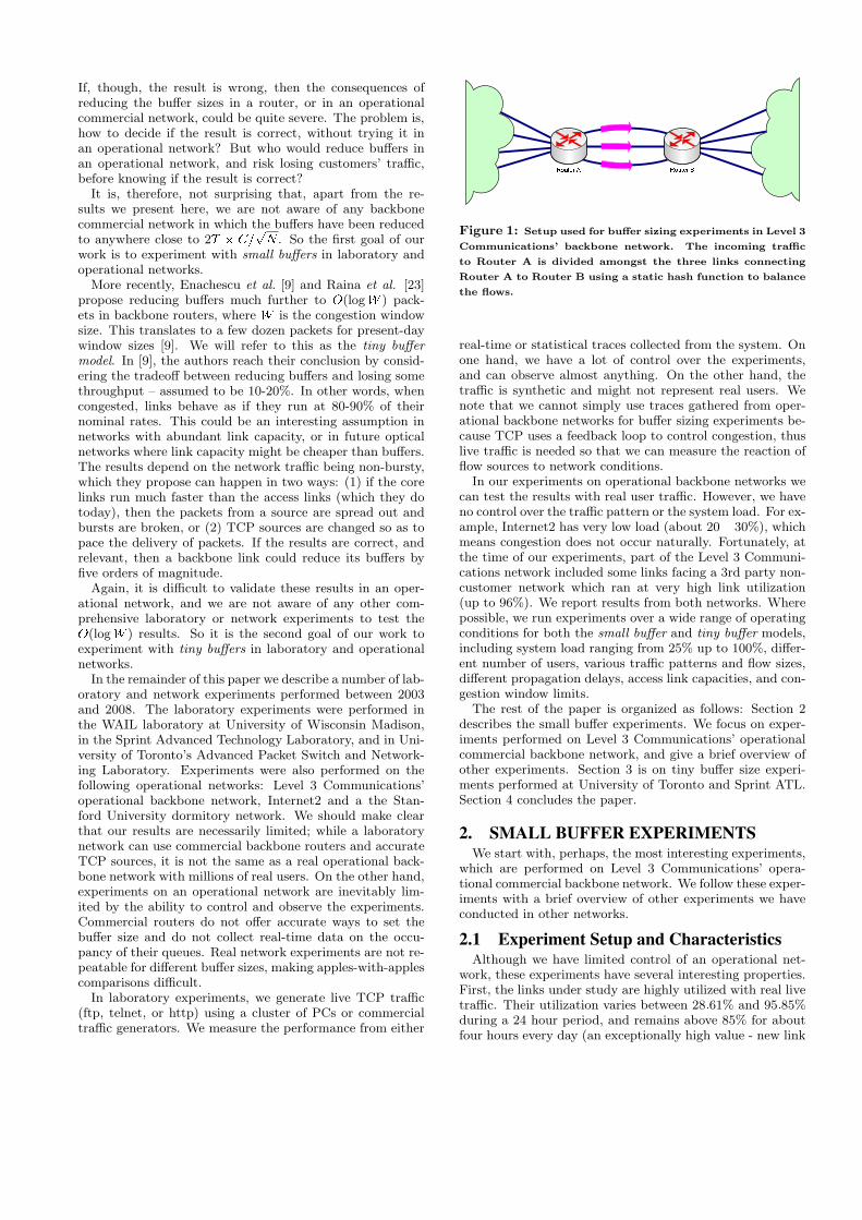
Figure 1: Setup used for buffer sizing experiments in Level 3
Communications’ backbone network. The incoming traffic
to Router A is divided amongst the three links connecting
Router A to Router B using a static hash function to balance
the flows.
real-time or statistical traces collected from the system. Onone hand, we have a lot of control over the experiments,and can observe almost anything. On the other hand, thetraffic is synthetic and might not represent real users. Wenote that we cannot simply use traces gathered from oper-ational backbone networks for buffer sizing experiments be-cause TCP uses a feedback loop to control congestion, thuslive traffic is needed so that we can measure the reaction offlow sources to network conditions.
In our experiments on operational backbone networks wecan test the results with real user traffic. However, we haveno control over the traffic pattern or the system load. For ex-ample, Internet2 has very low load (about 20� 30%), whichmeans congestion does not occur naturally. Fortunately, atthe time of our experiments, part of the Level 3 Communi-cations network included some links facing a 3rd party non-customer network which ran at very high link utilization(up to 96%). We report results from both networks. Wherepossible, we run experiments over a wide range of operatingconditions for both the small buffer and tiny buffer models,including system load ranging from 25% up to 100%, differ-ent number of users, various traffic patterns and flow sizes,different propagation delays, access link capacities, and con-gestion window limits.
The rest of the paper is organized as follows: Section 2describes the small buffer experiments. We focus on exper-iments performed on Level 3 Communications’ operationalcommercial backbone network, and give a brief overview ofother experiments. Section 3 is on tiny buffer size experi-ments performed at University of Toronto and Sprint ATL.Section 4 concludes the paper.
2. SMALL BUFFER EXPERIMENTSWe start with, perhaps, the most interesting experiments,
which are performed on Level 3 Communications’ opera-tional commercial backbone network. We follow these exper-iments with a brief overview of other experiments we haveconducted in other networks.
2.1 Experiment Setup and CharacteristicsAlthough we have limited control of an operational net-
work, these experiments have several interesting properties.First, the links under study are highly utilized with real livetraffic. Their utilization varies between 28:61% and 95:85%during a 24 hour period, and remains above 85% for aboutfour hours every day (an exceptionally high value - new link

capacity was added right after the experiments were com-pleted).
The link under study consists of three physical, load-balanced links (Figure 1). Traffic at the upstream routeris divided equally among the three physical links. Each in-coming flow is assigned to one of the three links using astatic hash function based on the source-destination IP andport numbers of the flow. Ideally, there is equal traffic oneach link (particularly as there are thousands of flows)1. Ifwe give each physical link a different amount of buffering,we can perform an apples-with-apples comparison betweendifferent buffer sizes under almost identical conditions.
The three physical links are OC-48 (2.5Gbps) links facinga 3rd party non-customer network, carrying Internet mixtraffic with an emphasis toward high speed consumer ac-cess. Assuming an average rate of 250Kbps per flow, eachlink carries about 10,000 flows when highly utilized2. Thedefault buffer size is 190ms per-link (60MB or 125,000 pack-ets assuming an average packet size of 500B). We reducethe buffer sizes to 10ms (about 3MB or 6,000 packets), 5ms(1.5MB or 3,000 packets), 2.5ms (750KB or 1,500 packets)and 1ms (300KB or 600 packets). Based on the small buffersize model, we can expect to need a buffer size of about2-6ms (depending on the actual value of N).
The buffer sizes are set for 5 days, so they capture theimpact of daily and weekly changes in traffic. The wholeexperiment lasts two weeks and was performed in March,2005. We gather link throughput and packet drop statisticswhich are collected by the router every 30 seconds from eachof the three links. It would be preferable to capture allpackets and recreate the time series of the buffer occupancyin the router, but the network does not have the facility todo this. Still, we are able to infer some interesting results.
We also actively inject test flows, measuring the through-put and drops, and compare the performance of the flowsgoing through different links to find out the impact of buffersize reduction. The amount of test flow traffic is kept small.It is worth noting that the network does not use traffic shap-ing at the edges or in the core. The routers do not use RED,and packets are dropped from the tail of the queue.
2.2 Experiment ResultsDuring the course of the experiments, we always keep the
buffer size on one link at its original size of 190ms and re-duce the buffer size on the other two links. Figure 2 showsthe packet drop rate as a function of system load for variousbuffer sizes. As explained before, both the load and droprates are measured in time intervals of 30 seconds, and eachdot in the graph represents one such interval. Figure 2(a)shows that we do not see a single packet drop using a buffersize of 190ms. Similarly, we observe no drops using either10ms or 5ms of buffering during the course of the experi-ments, which last more than 10 days for the 190ms buffersize, and about 5 days for each of the 10ms and 5ms buffersizes.
It is quite surprising that the buffer size can be reducedby a factor of forty without dropping packets even thoughthe utilization frequently exceeds 95%. It suggests thatthe backbone traffic is very smooth. Others also report
1In this case, the load balancing was not ideal, as we willexplain later.2This assumption is arbitrary based on what we assume tobe the average end-user bandwidth.
smoothness in traffic in core networks [13,14], despite some-what older results which show self-similarity in core traf-fic [10, 11, 24]. Whether this is a result of a shift in trafficpattern and network characteristics over time, or simply theconsequence of huge amounts of multiplexing, remains tobe determined. We find traffic to be extremely smooth inlaboratory and backbone networks when there are a largenumber of flows.
Figure 2(b) shows the drop rate as a function of load,when the buffer sizes is reduced to 2.5ms. This is in thelower part of the range defined by the small buffer sizingmodel, and, as expected, we start to observe some packetdrops. However, packet drops are still rare; less than 0.02%for the majority of samples. In two samples over five days,we see a packet drop rate between 0.02% and 0.04% and inone sample the drop rate is close to 0.09% 3.
Figure 2(c) shows what happens when we reduce the buffersize to 1ms. Here there are a lot more packet drops, which weexpect because the the buffer size is now about half the valuesuggested by the small buffer sizing model. It is interestingto note that almost all of the drops occur when the load isabove 90%, even though the load value is averaged over aperiod of 30 seconds. The instantaneous load is presumablyhigher, and the link must be the bottleneck for some of theflows. We conclude that having some packet drops does notlead to a reduction in available throughput; it appears thatTCP’s congestion control algorithms are functioning well.
Next we take a closer look at link utilizations over time.Figure 3(a) compares the link utilization for the links with190ms and 1ms of buffering, over three days, by plottingtheir ratio (i.e. relative utilization) as a function of time.Ideally, the utilization on both links would be equal at alltimes. However, the differences are not symmetric. The linkwith 1ms buffering has a slightly higher utilization for themajority of the time.
To further investigate the cause of this asymmetry, we plotlink utilizations as a function of time in Figure 3(b). By com-paring this graph with Figure 3(a) we observe that duringthe periods when the overall load of the system is high, thelink with 1ms has a slightly higher utilization than the linkwith 190ms. Figure 3(c) suggests the same, in a differentyet more precise way. Each dot in this figure, represents theutilization of the two links in a period of 30 seconds. We cansee that the majority of the dots fall below the 45 degree linein the graph, which suggests the link with 1 ms of bufferinghas a higher utilization.
The higher utilization with smaller buffers can be attributedto one of the following two reasons: (1) It might be due tohigher loads on the link with 1ms of buffering. Since we havemore drops on this link, sources need to send duplicates ofthe dropped packets, and that might be why we see a higherload. Or, (2) the load balancing scheme might be skewedand might divide the traffic somewhat unevenly among thethree links, thus directing more traffic to one of the links.
The question is which of the two reasons is the cause ofhigher link utilization on one of the two links? The easiestway to answer this question would be swapping the buffersizes on the two links under study. Unfortunately, immedi-
3It would be very interesting to take a closer look at howpacket drops are distributed over time. Unfortunately, givenour limited measurement capabilities in a commercial infra-structure, we cannot study the distribution of packet dropsover time granularities finer than 30 seconds.

0
0.04
0.08
0.12
0.16
0.2
0 20 40 60 80 100
Load (%)
Pa
ck
et
Dro
p R
ate
(%
)
0
0.04
0.08
0.12
0.16
0.2
0 20 40 60 80 100
Load (%)
Pa
ck
et
Dro
p R
ate
(%
)
0
0.04
0.08
0.12
0.16
0.2
0 20 40 60 80 100
Load (%)
Pa
ck
et
Dro
p R
ate
(%
)
(a) (b) (c)
Figure 2: Packet drop rate as a function of load for different buffer sizes. (a) For a buffer size of 190ms we observe no packet
drops. Although not shown here, there is also no drops with either 10ms or 5ms of buffering. (b) For a buffer size of 2.5ms
packet drops occur in only a handful of cases. (c) When the buffer size is set to 1ms we observe packet drops during high
utilization time periods.
0.90
0.95
1.00
1.05
1.10
1.15
1.20
Time
Re
lati
ve
Uti
liza
tio
n
Day 1 Day 3Day 220
30
40
50
60
70
80
90
100
Time
Uti
liza
tio
n (
%)
Buffer 1ms Buffer 190ms
Day 1 Day 3Day 2 20
40
60
80
100
20 40 60 80 100
Utilization (%) - link with 1ms buffer
Uti
liza
tio
n (
%)
- lin
k w
ith
19
0m
s b
uff
er
(a) (b) (c)
Figure 3: Comparing the utilization of the links with 1ms and 190ms of buffering. (a) Link utilization using 1ms buffering
relative to 190ms buffering. (b) Individual link utilizations over time. (c) Utilization of 1ms buffer link vs. the utilization of
the 190ms buffer link.
ately after our experiments, Level 3 upgraded the networkand added extra capacity to reduce the load on the links wewere studying, which means we could not repeat the exper-iment with the same conditions.
Interestingly, we see the same phenomena (higher utiliza-tion in one link than the others) when the buffer sizes areset to 190ms, and 5ms on two links. Since we do not haveany packet drops in these cases, buffer occupancies in bothlinks cannot be affected by packet drops, the RTT of flowsmust be the same in both links, and therefore (1) cannot bethe reason here, i.e. any difference in utilization is mostprobably not a result of the reaction of TCP sources topacket drops4. In other words, we associate these slight dif-ferences between link utilizations with imperfections in theload balancing scheme deployed in the system, rather thanthe changes in buffer sizes. We conclude that reducing buffersizes in this network does not have a significant impact onthe performance.
4Based on our experiment results, the load balancing schemeused in this system was changed to one which is believed tobe more fair in distributing the load.
2.3 Other Small Buffer ExperimentsOther than the experiments on Level 3 Communications’
backbone network, we have also conducted some other ex-periments with the small buffer sizing model. These experi-ments include University of Wisconsin Madison’s AdvancedInternet Laboratory (WAIL), and Stanford University’s dor-mitory network.
In the WAIL experiment, already reported by Appenzelleret al. [4], a cluster of PCs is used to generate up to 400 liveTCP flows, and the traffic is directed to a Cisco GSR router.The buffer sizes on the router is reduced by a factor of 10-20, which does not result in any degradation in the systemthroughput.
In the Stanford University experiment, we use a CiscoVXR 7200 which connects the dormitories to the Internetvia a 100Mbps link. Traffic is from a mix of different appli-cations including web, ftp, games, peer-to-peer, streamingand others, and we have 400-1900 flows at any given time.The buffer sizes on the router are reduced by a factor of 20with no impact on network throughput. We omit the de-tails of these experiments due to limited space and refer theinterested reader to [15] for more details. All of these ex-periments are inline with the small buffers theory, which isbased on loose assumptions on the number of flows and their

independence. We are fairly confident that the O(C=pN)
will hold quite generally for backbone routers.
3. TINY BUFFER EXPERIMENTSIn this section we describe our experiments performed in
the context of the tiny buffer model: i.e. we consider a singlepoint of congestion, assume core links run much faster thanthe access links, and expect a 10-20% reduction in networkthroughput. Without a guarantee that these conditions holdin an operational backbone network, it is not feasible to testthe tiny buffer model, and, therefore, we have to contentourselves to laboratory experiments. We understand this isa limiting factor, and view our work as a first pass in a morecomprehensive experimental study of the tiny buffer sizingmodel by us and others.
3.1 University of Toronto ExperimentsWe perform an extensive set of experiments on tiny buffer
sizing at University of Toronto’s Advanced Packet Switchand Networking Laboratory. The goal is to study the impactof tiny buffers on network performance and to identify con-ditions under which tiny buffers are sufficient. During thecourse of our experiments, we vary several network parame-ters such as buffer size in routers, packet injection times, andhardware level parameters. The performance metrics thatwe study are link utilization, an important factor from Inter-net Service Providers’ point of view, as well as loss and flowcompletion times, which are major concerns of end-users.
3.1.1 Experiment Setup
Performing time-sensitive network experiments is extremelydifficult, especially in the context of tiny buffers, mainly be-cause creating a network with a topology that is representa-tive of a real backbone network requires significant resources.During the course of our experiments, we encounter sev-eral challenges, including generating realistic network traffic,emulating delay, approximating large topologies, collectinghigh-resolution packet-level measurements, and accountingfor scaling approximations. In general, these factors, alongwith hardware/software configuration and limitations, canhave a large influence on an experiment’s outcome. In [5]we study the challenges associated with performing time-sensitive network experiments in a test-bed. We provideguidelines for setting up test-beds, paying particular atten-tion to those factors that may affect the accuracy of exper-imental results, and describe obstacles encountered duringour own experiments. Below we summarize the importantfactors for our tiny buffers experiments.
Traffic Generation: As mentioned above, generatingrealistic traffic is one of the key challenges in modeling anetwork. Experiments in a laboratory setup often use mul-tiple hosts as traffic generators. However, creating a largenumber of connections, in order to model traffic in networkscloser to the core of the Internet, with thousands of flows,is not a trivial task. In our experiments, the traffic is gen-erated using the open-source Harpoon traffic generator [25].We use a closed-loop version [22] of Harpoon, modified byresearchers at the Georgia Institute of Technology. It isshown in [21] that most Internet traffic (60-80%) conformsto a closed-loop flow arrival model. In this model, a givennumber of users (running at the client hosts) perform suc-cessive TCP requests from the servers. The size of eachTCP transfer follows a specified random distribution. Af-
ter each download, the user stays idle for a thinking periodwhich follows another distribution. We also made severalfurther modifications to the closed-loop Harpoon: each TCPconnection is immediately closed once the transfer is com-plete, the thinking period delay is more accurately timed,and client threads with only one TCP socket use blocking in-stead of non-blocking sockets. For the transfer sizes, we usea Pareto distribution with mean 80KB and shape parameter1.5. These values are realistic, based on comparisons withactual packet traces [22]. The think periods follow an expo-nential distribution with a mean duration of one second. Weperform extensive experiments to evaluate Harpoon’s TCPtraffic; the results are provided in the Appendix.
Switching and Routing: One of the major problemswe encountered while performing buffer sizing experimentsis that commercial routers do not allow precise adjustmentof their buffer sizes. Moreover, they are not able to providea precise buffer occupancy time-series, which is essential forstudying buffer sizing. To address these issues, we use aprogrammable network component called NetFPGA [2] asthe core element of our test-bed. NetFPGA is a PCI formfactor board that contains reprogrammable FPGA elementsand four Gigabit Ethernet interfaces. Incoming packets toa NetFPGA board can be processed, possibly modified, andsent out on any of the four interfaces. Using a NetFPGA asa router allows us to precisely set the buffer sizes to a specificnumber of either bytes or packets, and the openness of theNetFPGA platform avoids the dangers of hidden buffers thatmay exist in commercial routers.
Traffic Monitoring: Obtaining the exact queue occu-pancy, the packet loss rate and the bottleneck link utiliza-tion over time is vital for experiments involving small packetbuffers, which are extremely sensitive to packet timings. Un-fortunately, to the best of our knowledge, no commercialrouter provides these metrics today. However, we added amodule to the NetFPGA-based router that records an eventeach time a packet is written to, read from or dropped byan output queue [5]. Each event includes the packet sizeand the precise time that it occurred, with an 8 nanosecondgranularity. These events are gathered together into eventpackets, which can be received and analyzed by the com-puter hosting the NetFPGA board or another computer onthe network. The event packets contain enough informationto reconstruct the exact queue occupancy over time and todetermine the packet loss rate and bottleneck link utiliza-tion. The resulting data is at a previously unobtainable levelof precision, which is invaluable for our experiments.
Packet Pacing: The tiny buffer model assumes networktraffic is paced. This happens naturally if we have slowaccess links. As packets of a TCP flow cross the boundariesof slow access links (usually operating at a few Mbps) tohigh capacity core links (operating at tens of Gbps) they areautomatically spaced out. However, if access links are fast,sources need to implement Paced TCP [23], which spacesout packets as they leave the source.
To study the necessity of the pacing assumption in the tinybuffer model, we perform experiments with paced and non-paced traffic. We use the Precise Software Pacer (PSPacer) [26]package to create the paced traffic by emulating multipleslower access links at each server. The PSPacer package isinstalled as a loadable kernel module for the Linux platformand provides precise network bandwidth control and trafficsmoothing. In the non-paced experiments, we make no ef-

Servers Clients
Delay emulator GigE switch
1 Gbps
bottleneck
NetFPGA router
Servers
Bottleneck router
Clients
(1)
(2)
(1)
(2)
(3)
(4)
(3)
(4)
Delay emulatorsNetFPGA routers GigE switches
(a) (b)
Figure 4: Topologies of the network used in our experiments. The capacity of all links is 1Gbps.
fort to pace the traffic. Both experiments use an unmodifiedversion of TCP, as implemented by the Linux network stack.
Packet Delay: To emulate the long Internet paths ina test-bed it is necessary to artificially delay every packet.We route all traffic through a host running NISTNet [7], anetwork emulator, to introduce propagation delays in thepackets that flow from the clients to the servers. The NIST-Net host is neither a client nor a server in the experiment.
The traffic at the delay emulator machine is monitoredusing tcpdump, which captures the headers of every packet.In some circumstances, under high-load tcpdump may notcapture a packet, however we observe that the number ofsuch missed packets is negligible: less than 0.1% of the totalpackets. We use these packet traces to measure the flowcompletion times and per-flow packet interarrival times.
Topologies: Due to limitations in a laboratory environ-ments, we have to content ourselves with a limited set oftopologies. Our experiments are conducted in two differenttopologies. In the first one, shown in Figure 4(a), a singlepoint of congestion is formed, where packets from multipleTCP flows go through the NetFPGA router, and share abottleneck link toward their destinations. Throughout dif-ferent sets of experiments, we change the size of the outputbuffer in the NetFPGA router, and study how the buffer sizeaffects the utilization and loss rate of the bottleneck link aswell as the flow completion times. As mentioned before,the necessity of smooth traffic is investigated by changingthe bandwidth of access links in the network. Our secondtopology is illustrated in Figure 4(b), where the main traf-fic (traffic on the bottleneck link) is mixed with some crosstraffic, and is separated from the cross traffic before goingthrough the bottleneck link. The goal is to determine howthe main traffic is affected by the cross-cut traffic.
In our experiments, we mostly use the dumb-bell shapedtopology. This is typical in the congestion control literaturefor two main reasons. First, there is a very small chance ofhaving more than one point of congestion along any source-destination path. Once a link on the path is congested,flows on that path are limited in rate, and thus cannot in-crease to congest another link along the path. Second, theclient/server nodes and the links connecting them to the bot-tleneck link in the dumb-bell shaped topology can represent
a path connecting source nodes to the bottleneck link in areal topology. Based on these two reasons, as well as the dif-ficulties associated with performing accurate time-sensitivenetwork experiments, we mainly consider dumb-bell shapedtopology as a representative of more generic networks. How-ever, we understand the limitations of this approach andthat it may suffer from problems such as those noted in [12].We hope to study the impact of other topologies with mul-tiple points of congestion in the future.
Host Setup: In all sets of the experiments, we use TCPNew Reno with the maximum advertised TCP window sizeset to 20MB, so that data transferring is never limited by thewindow size. The path MTU is 1500 bytes and the serverssend maximum-sized segments. The aggregated traffic goesto the NetFPGA router over the access links, and from therouter to the client network over the 1Gbps bottleneck link.The Linux end-hosts and the delay emulator machines areDell Power Edge 2950 servers running Debian GNU/Linux4.0r3 (codename Etch) and use Intel Pro/1000 Dual-portGigabit network cards.
3.1.2 Experiment Results
In this section, we provide the results of our experimentalstudies on tiny buffers. We report network performance,including utilization of the bottleneck link, loss rate, andflow completion times for TCP traffic.
To study the impact of tiny buffers on performance, werun two sets of experiments, paced and non-paced, using thetopology shown in Figure 4(a) with various router output-buffer sizes. Slower access network bandwidths are emulatedusing PSPacer with flows on a single machine grouped intoclasses. All flows belonging to the same class share a singlequeue with a service rate set to 200 Mbps. The size ofthe queue is chosen to be large enough (5000 packets) thatthere are no drops at these queues. Because the router’sinput/output links are 1Gbps, the emulated slow access linksspread out the bursts in the router’s aggregate ingress traffic.Initially, we observed an increased RTT during the pacedexperiments because our method of pacing forces packetsto wait in queues which are serviced at a slower rate. Tomake the two cases more comparable we increase the delayintroduced by NISTNet in the non-paced case so that the

�.3
0.4
0.5
0.6
0.7
0.8
0.9
1
0 50 100 150 200 250 300 350 400
Buffer size (pkts)
Lin
k U
tilizati
on
1200 Flows-paced
1200 Flows-nonpaced
2400 Flows-paced
2400 Flows-nonpaced0
1
2
3
4
5
6
0 50 100 150 200 250 300 350 400
Buffer size (pkts)
Lo
ss r
ate
(%
)
1200 Flows-paced
1200 Flows-nonpaced
2400 Flows-paced
2400 Flows-nonpaced
(a) (b)
0.5
0.6
0.7
0.8
0.9
1
1.1
1.2
1.3
1.4
1.5
0 50 100 150 200 250 300 350 400
Buffer size (pkts)
Av
era
ge
flo
w c
om
ple
tio
n t
ime
fo
r .
sh
ort
flo
ws
(s
ec
)
1200 Flows-paced
1200 Flows-nonpaced
2400 Flows-paced
2400 Flows-nonpaced
0
2
4
6
8
10
12
14
16
0 50 100 150 200 250 300 350 400
Buffer size (pkts)
Avera
ge f
low
co
mp
leti
on
tim
e f
or
lon
g f
low
s (
sec)
1200 Flows-paced
1200 Flows-nonpaced
2400 Flows-paced
2400 Flows-nonpaced
(c) (d)
Figure 5: (a) Link utilization as a function of buffer size for paced and non-paced experiments. (b) Loss rate as a function
of buffer size for paced and non-paced experiments. (c) Average flow completion times for short-lived flows. (d) Average flow
completion times for long-lived flows.
RTT is roughly 130 ms in both cases. The results shownin Figure 5 and analyzed in the following sections are theaverage of ten runs. The run time for each experiment is twominutes. To avoid transient effects, we analyze the collecttraces after a warm-up period of one minute.
For each experiment we change the size of the outputbuffer in the NetFPGA router and investigate how the buffersize affects both the utilization and loss rate of the bottle-neck link as well as the flow completion times.
Performance: Figure 5(a) shows the effect of changingthe buffer size on the average utilization of the bottlenecklink. The total number of flows sharing the bottleneck link is1200 and 2400. In both cases, pacing results in significantlylarger utilization when the buffer size is very small – smallerthan 10-50 packets. For example, with 1200 flows, pacingincreases the utilization from about 45% to 65% when thebuffer size is only 10 packets and it increases the utilizationfrom about 65% to 80% when we have 2400 flows in thesystem (The improvement is roughly 20% in both cases).This difference gets smaller as the buffer size increases.
Note that with 1200 flows, in both paced and non-pacedcases the link utilization does not achieve higher than 65%.This is the maximum offered load to the link since in thiscase the think time and file size distribution parameters donot create enough active users to saturate the bottleneck link(we observed that the number of active users is roughly halfthe total users). Most of these active users are setting up
many short connections which have very small throughput(almost about 6 packets per RTT) and thus they cannotnecessarily saturate the link. Assuming that the averagetransmission rate is 6 packets per RTT, the total utilizationwould be roughly 600 (active) � 6 (packets) � 1500 � 8(MTU) / 0.130 (RTT) which is only about 330 Mbps. Theplot shows larger amount (about 650 Mbps) because not allof the flows are this small and hence there are some flowsthat are sending at a higher rate.
Another interesting observation is that with paced traffic,the link utilization appears to be independent of the buffersize while this is not the case for non-paced traffic. Thus,with paced traffic, there is no need to increase the bufferingto achieve a certain link utilization.
Interestingly, we observe that in the 2400 flows case, in-creasing the buffer size makes the paced traffic’s link uti-lization lower than the non-paced traffic’s. This has alreadybeen observed and reported in [3] and [28]. The main rea-son is the trade-off between fairness and throughput. In thecase where there are many paced flows and the buffer size islarge, at the point where the buffer is almost full, each flowis sending paced packets at each RTT. These packets getmixed with other flows in a paced manner before arriving atthe bottleneck router, and, if the buffer is already full andnumber of flows in the network is large, many of flows willexperience a loss event and reduce their congestion windowby half. Although it seems fair that the packet drops should
be spread among many flows, it may cause the bottlenecklink’s utilization to drop. However, with non-paced traffic,since packets arrive at the bottleneck link in large bursts, asmaller number of unlucky flows will hit the full buffer, willexperience the loss event, and will reduce their rate. Thisis unfair for the few flows that reduce their rate, but it willkeep the link utilization high.
Figure 5(b) compares the loss rate as a function of buffersize for paced and non-paced traffic. We can see that similarto link utilization, for paced traffic the loss rate is almost in-dependent of buffer size, whereas it decreases exponentiallywith non-paced traffic. For tiny buffers, there is a notablereduction in the loss rate for both 1200 and 2400 flow cases.With 1200 flows, the link is not saturated and hence theloss rate for paced traffic is always less than 0.01%. How-ever, with tiny buffers, non-paced traffic experienced around2% drop in average.
Flow Completion Time: To address the question ofhow tiny buffers may affect an individual flow’s completiontime, we collect the start and finish times of all the flowsgoing through the bottleneck link, and find the average com-pletion time separately for short and long-lived flows. Wedefine a short-lived flow to be a flow which never exits theslow-start mode. Long-lived flows are those which enter thecongestion avoidance mode. We consider flows smaller than50 KB (roughly 33 packets) as short-lived flows and flowslarger than 1000 KB (roughly 600 packets) as long-livedflows. If there is no loss, it takes less than 6 RTTs for theshort flows to be completed.
Figures 5(c) and 5(d) show the average flow completiontimes for short-lived and long-lived flows, respectively. Asthe plots show, with 1200 paced flows, the flow completiontime is independent of the buffer size for both short andlong-lived flows, whereas with non-paced traffic, increasingthe buffer size reduces the flow completion times. In thiscase, the flow completion time of the paced traffic is alwayssmaller than that of the non-paced traffic (for both short-and long-lived flows) and there is a notable difference be-tween flow completion times for long-lived flows with tinybuffers. With 2400 flows, the average flow completion timeof the paced traffic is always less than that of the non-pacedtraffic in the tiny buffers region and they are almost equalwith buffers larger than 50 packets.
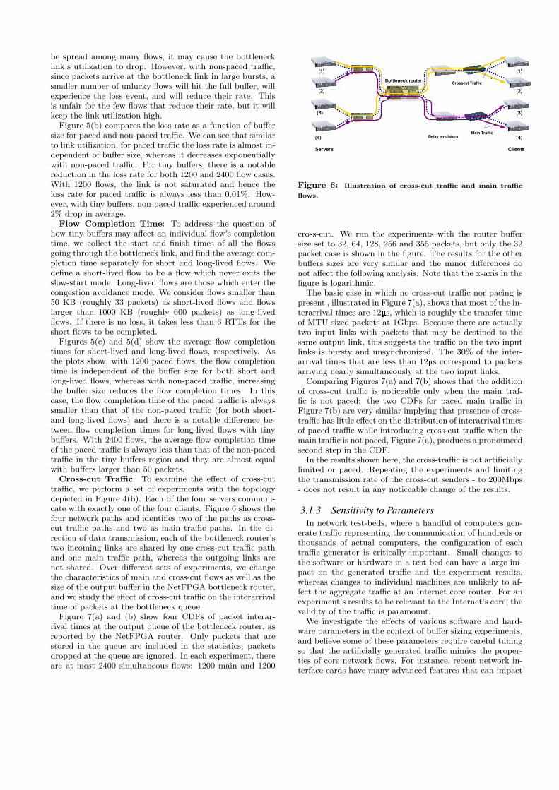
Cross-cut Traffic: To examine the effect of cross-cuttraffic, we perform a set of experiments with the topologydepicted in Figure 4(b). Each of the four servers communi-cate with exactly one of the four clients. Figure 6 shows thefour network paths and identifies two of the paths as cross-cut traffic paths and two as main traffic paths. In the di-rection of data transmission, each of the bottleneck router’stwo incoming links are shared by one cross-cut traffic pathand one main traffic path, whereas the outgoing links arenot shared. Over different sets of experiments, we changethe characteristics of main and cross-cut flows as well as thesize of the output buffer in the NetFPGA bottleneck router,and we study the effect of cross-cut traffic on the interarrivaltime of packets at the bottleneck queue.
Figure 7(a) and (b) show four CDFs of packet interar-rival times at the output queue of the bottleneck router, asreported by the NetFPGA router. Only packets that arestored in the queue are included in the statistics; packetsdropped at the queue are ignored. In each experiment, thereare at most 2400 simultaneous flows: 1200 main and 1200
Servers
Bottleneck router
Clients
(1)
(2)
(1)
(2)
(3)
(4)
(3)
(4)
Crosscut Traffic
Main TrafficDelay emulators
Figure 6: Illustration of cross-cut traffic and main traffic
flows.
cross-cut. We run the experiments with the router buffersize set to 32, 64, 128, 256 and 355 packets, but only the 32packet case is shown in the figure. The results for the otherbuffers sizes are very similar and the minor differences donot affect the following analysis. Note that the x-axis in thefigure is logarithmic.
The basic case in which no cross-cut traffic nor pacing ispresent , illustrated in Figure 7(a), shows that most of the in-terarrival times are 12µs, which is roughly the transfer timeof MTU sized packets at 1Gbps. Because there are actuallytwo input links with packets that may be destined to thesame output link, this suggests the traffic on the two inputlinks is bursty and unsynchronized. The 30% of the inter-arrival times that are less than 12µs correspond to packetsarriving nearly simultaneously at the two input links.
Comparing Figures 7(a) and 7(b) shows that the additionof cross-cut traffic is noticeable only when the main traf-fic is not paced: the two CDFs for paced main traffic inFigure 7(b) are very similar implying that presence of cross-traffic has little effect on the distribution of interarrival timesof paced traffic while introducing cross-cut traffic when themain traffic is not paced, Figure 7(a), produces a pronouncedsecond step in the CDF.
In the results shown here, the cross-traffic is not artificiallylimited or paced. Repeating the experiments and limitingthe transmission rate of the cross-cut senders - to 200Mbps- does not result in any noticeable change of the results.
3.1.3 Sensitivity to Parameters
In network test-beds, where a handful of computers gen-erate traffic representing the communication of hundreds orthousands of actual computers, the configuration of eachtraffic generator is critically important. Small changes tothe software or hardware in a test-bed can have a large im-pact on the generated traffic and the experiment results,whereas changes to individual machines are unlikely to af-fect the aggregate traffic at an Internet core router. For anexperiment’s results to be relevant to the Internet’s core, thevalidity of the traffic is paramount.
We investigate the effects of various software and hard-ware parameters in the context of buffer sizing experiments,and believe some of these parameters require careful tuningso that the artificially generated traffic mimics the proper-ties of core network flows. For instance, recent network in-terface cards have many advanced features that can impact

0
0.2
0.4
0.6
0.8
1
1000 10000 100000
Interarrival Time (nanosecond)
CD
F
Non-paced main with cross-cut
Non-paced main without cross-cut
0
0.2
0.4
0.6
0.8
1
1000 10000 100000
Interarrival Time (nanosecond)
CD
F
Paced main with cross-cut
Paced main without cross-cut
(a) (b)
Figure 7: CDF of interarrival times at the output queue of the bottleneck router in cross-cut topology: (a) main traffic is
non-paced, b) main traffic is paced.
the shape of the output traffic, or measurement of variousperformance metrics. Due to space limitations we describeonly two such parameters here, which we believe have thehighest impact on our results, and refer the interested readerto [5].
TCP Segmentation Offload (TSO): With TSO en-abled, the task of chopping big segments of data into packetsis done on the network card, rather than in software by theOperating System. The card sends out the group of packetsthat it receives from the kernel back to back, creating burstyand un-mixed traffic. Clearly, this makes the traffic burstyand highly impacts the results of buffer sizing experimentsin a test-bed. Also, TSO must be disabled if packets are be-ing paced in software. When TSO was enabled during ourexperiments, the gaps between packets added by PSPacer,described in Section 3.1.1, were only added between the largegroups of packets sent to the network card, and the resultingtraffic on the wire did not have a gap between each packet.Instead, it contained a group of packets back to back fol-lowed by a small gap, which was drastically different fromthe intended traffic pattern.
Interrupt Coalescing (IC): To lower the CPU’s inter-rupt servicing overhead, network cards can coalesce the in-terrupts caused by multiple events into a single interrupt.With receiver IC enabled, the interarrival time of packetsare changed. The network card will delay delivering packetsto the operating system while waiting for subsequent packetsto arrive. Not only does this affect packet timing measure-ments, but, due to the feedback in network protocols likeTCP, it can also change the traffic’s shape [19].
3.2 Sprint ATL ExperimentsOur second set of tiny buffers experiments is conducted
in collaboration with Sprint ATL. Figure 8 shows the topol-ogy of the emulated network, which is similar to the settingconsidered in tiny buffer sizing model [9]. The core of the ex-periments is a Juniper T640 router, whose buffers are modi-fied throughout the study5. The router is connected to fourdifferent networks through four Gigabit Ethernet interfaces.
5We tried several other routers including Cisco GSR 12000,and Juniper M160. For the buffer sizes we were interestedin this experiment, Juniper T640 seemed to be the mostsuitable choice (for details see [15]).
Each cloud in Figure 8 represents one of these networks. Thecloud on the left contains all the users/clients, and the threeclouds on the right hold the servers. Each server belongsto one of the 99 different subnets (33 for each of the threeserver networks). The capacity of the access link connectingeach server to the rest of the network is set to 15Mbps bydefault. The requests for file downloads flow from left toright (from clients to servers), and the actual files are sentback from right to left. In this direction, the router has threeingress and one egress line, which means by increasing theload we are able to create congestion on the link connectionT640 router to the client network.
In practice, the clients and servers are emulated by twodifferent boxes: Spirent Communications’ Avalanche boxplays the role of clients, and the Reflector box plays therole of servers (Figure 9). Each box has four Gigabit Eth-ernet Interfaces. Obviously, we use only one interface fromthe Avalanche box, and three interfaces from the Reflectorbox to connect the boxes to the T640 router. These linkscorrespond to core links, and the link connecting the routerto the Avalanche box is the target link. The access links areemulated by the Reflector box, which allows us to changethe access link capacity to any desired value6. The delayassociated with each access link is also emulated by the Re-flector box. Since all other link delays are negligible, we cancontrol the two-way propagation delay of packets by modi-fying these values. In the Appendix, we explain the resultsof evaluation tests on Avalanche’s TCP traffic
Throughout the experiments, we use IPMon systems [1] tocapture the headers of all the packets which go through thelinks connecting the router to the Avalanche and Reflectorboxes. These headers are recorded along with high preci-sion time-stamps. By matching the packet traces on ingressand egress lines of the router, we can measure the time eachpacket has spent inside the router, and thus, we can cal-culate the time-series representing the queue occupancy ofthe router. This also helps us identify any undocumented
6In the Internet, access links are slow on client side. Wefound out Avalanche does not enforce rate limitations forincoming traffic, and had to push slow accesses to the serverside in this experiment so that we can emulate the impactof slow access links. Avalanche has some other minor timingissues which are described in the Appendix.

1Gb/s
1Gb/s
1Gb/s
Subnet 1
Subnet 33
1Gb/sSubnet 34
Subnet 66
Subnet 67
Subnet 99
Juniper T640 Router
Clients
Servers
15Mb/s
Figure 8: Topology of the network used in experiments.
The capacity of core links is 1Gbps, and the capacity of access
links is 15Mbps.
Figure 9: Sprint ATL’s tiny buffer experiment setup.
buffers inside the router. Such buffers could be fixed-delaybuffers (e.g. part of a pipeline, or staging buffers), or couldbe additional FIFO queues.
3.2.1 Experiment Results
In this section we study the impact of changing buffersizes on network performance. When allowed by our testingequipment, we also study the effect of changing some othernetwork properties (like traffic patterns, access link proper-ties, number of flows, and others) on buffer sizing results.Due to lack of space, we review some of our results here,and refer the interested reader to [15] for details.
Performance: We reduce the buffer sizes on the routerfrom 8500 packets to just 50 packets, and measure the through-put, drop rate, and delay observed by individual packets asperformance metrics. At 1Gbps line speed, and an RTTof 50ms, 8500 packets is about twice the bandwidth-delayproduct, and 50 packets lies in the range of the tiny buffersizing model.
In this experiment we increase the number of users from 0to 600 during a period of 50 seconds, and keep the number ofusers at 600 for 5 minutes, measuring throughput, delay, anddrop rate during this time interval7. Each user downloadsa 1MB file from an ftp server. Once the file download iscompleted the user immediately starts downloading another
7The number 600 of users is chosen so that the effective loadof the system is about 100%.
file. The average RTT of the system is 50ms (more precisely15 +U [0; 20] on each of the forward and reverse paths), andthe capacity of access links connecting servers to the systemis 15Mbps. Both the server and clients have an advertisedcongestion window size of 16KB.
Figure 10(a) illustrates throughput as a function of timefor various buffer sizes, and Figure 10(b) represents the av-erage throughput for different buffer sizes. If we considerthe overhead of packet headers, the maximum throughputwe can get is about 950Mbps. We can see that a buffer sizebetween 8500 and 922 packets, gives a throughput of about100%. This is the range between the rule-of-thumb and thesmall buffer model. When we push the buffer size to 192,63, and 50 packets, which is in the range of tiny buffersmodel, the throughput goes down by 10%, as predicted the-oretically. The average level of throughput is maintainedvery smoothly throughout the experiments, as seen in Fig-ure 10(a).
Figure 10(c) shows that on average packets go through adelay of 155�s to 4.5ms (equivalent to 13 and 375 packets)for buffer sizes between 50 and 8500 packets. The aver-age packet delay is considerably smaller than the maximumbuffer size when it is set to 8500 packets. This is very similarto what we observed in Level 3 Communications’ network.The average delay increases as the buffer size is increasedfrom 50 to 1017 packets, and is slightly reduced for 8500packets. Since the packet drop rate is close to zero whenbuffer size is set to 1017 or 8500 packets, we expect these twoto have similar average delays, and the observed reductionin average delay might be a result of activation/deactivationof some hidden buffer inside the router.
For buffer sizes between 922 and 8500 packets, the droprate is very close to zero (Figure 10(d)). As expected, inthese cases utilization is close to 100%. For smaller bufferswe see a packet drop rate of up to 0.75%; only 0.25% morethan a M/D/1 queue of similar size and arrival rate, con-firming once more the smoothness of traffic going throughthe router.
The impact of increasing network load: In the previ-ous experiment, parameters were chosen so that the effectivesystem load is very close to 100%. What happens if we keepincreasing the load? Does the throughput of the networkcollapse as a result of congestion? This is a valid concern,and to find out the answer we perform another set of exper-iments. This time, we vary the potential load of the systembetween 25% and 150% 8. We control the system load bylimiting the access link rates and advertised congestion win-dow, and by changing the number of end users from 150 to1200.
Figure 11(a) plots the throughput of the system as a func-tion of load and various buffer sizes in this scenario. For anygiven buffer size increasing the potential load monotonicallyincreases the throughput. For large buffers, the throughputreaches 100% (950Mbps) when the potential load is 100%,and remains at that level for increased potential load. Forsmaller buffers, the throughput reaches 90%-95% as we in-crease the potential load from 25% to 100%, and remainsalmost fixed beyond that point. This is good news in the
8The potential load of the system is defined as the utilizationachieved when the bottleneck link capacity is increased toinfinity, and when the throughput is limited by other factors(like the maximum congestion window size, RTT, and accesslink capacities)

0
100
200
300
400
500
600
700
800
900
1000
0 50 100 150 200 250 300 350 400
Time (sec)
Thro
ughput
(Mb/s
)
50 Pkts 63 Pkts 192 Pkts 922 Pkts 8500 Pkts
85
90
95
100
50 63 192 922 1017 8500
Buffer Size (Packets)
Avera
ge T
hro
ug
hp
ut
(%)
950
902.
855
807.
Avera
ge T
hro
ug
hp
ut
(Mb
/s)
(a) (b)
0
1
2
3
4
5
6
50 63 192 922 1017 8500
Buffer Size (Packets)
Dela
y (
Mill
isecond)
0
0.1
0.2
0.3
0.4
0.5
0.6
0.7
0.8
0.9
1
50 63 192 922 1017 8500
Buffer Size (Packets)
Dro
p R
ate
(%
)
(c) (d)
Figure 10: (a) Throughput vs. time for various buffer sizes. (b) Average throughput vs. buffer size. (c) Delay statistics vs.
the buffer size. The red square represents the average delay and the bar represents the standard deviation. (d) Drop rate vs.
buffer size.
sense that we do not see a collapse in throughput as a resultof increased congestion. For a core network a potential loadbeyond 100% is very unlikely given that core networks areusually highly over-provisioned.
Performance as a function of the number of flows:We would like to see whether the number of flows affectsthe performance of the system. We cannot simply modifythe number of flows, since the potential load to the systemchanges with the number of flows. To fix this problem, weadjust the maximum congestion window size to keep thepotential load fixed, when modifying the number of flows inthe network. For 150 flows, the maximum congestion win-dow size is set to 64KB. As we increase the number of flowsto 300, 600, and 1200, we reduce the maximum congestionwindow size accordingly (to 32KB, 16KB, and 8KB). Thebuffer size is set to 85 packets in all these experiments.
Figure 11(b) illustrates the changes in network through-put as we increase the number of flows. When the numberof flows is very low (i.e. 150-300) the system throughputis significantly less than 100%. Even when we increase thecongestion window size (to increase the potential load), thesystem throughput is not significantly increased. This canbe explained by tiny buffer sizing model as follows: when thenumber of flows is low, we will not have a natural pacing asa result of multiplexing, and therefore, the throughput willnot reach 100%9. When the number of flows is large (i.e.
9This problem can be fixed by modifying traffic sources to
600-1200), the system throughput easily reaches 90-95%, in-dependent of the number of flows.
Increasing the number of flows beyond a few thousand canresult in a significant reduction in throughput, as the aver-age congestion window size becomes very small (2-3 packetsor even less), resulting in a very high drop rate and poor per-formance [8, 18]. This problem is not associated with tinybuffers, and unless we significantly increase the buffer sizeseven more than the rule-of-thumb it would not be resolved.We believe this is a result of poor network design and in-creasing the buffer sizes is not the right way to address suchissues.
We also conducted experiments to study the impact oftiny buffers on performance in the presence of different flowsizes, various access link capacities, and different distribu-tions of RTTs. Our results show the performance of a routerwith tiny buffers is not highly impacted by changes in theseparameters. For the sake of space, we omit the details andrefer the interested reader to [15].
3.3 Other Tiny Buffer ExperimentsOur tiny buffer experiments have been verified indepen-
dently in other test-beds at Alcatel-Lucent Technologies andVerizon Communications. The only operational network ex-
use Paced TCP. Here we do not have the tools to test this.The commercial traffic generator which we use does not sup-port Paced TCP.

0
100
200
300
400
500
600
700
800
900
1000
0 20 40 60 80 100 120 140
Potential Load (%)
Thro
ughput
(Mb/s
)
50 Pkts 63 Pkts 85 Pkts 192 Pkts 922 Pkts
1017 Pkts 8500 Pkts
0
10
20
30
40
50
60
70
80
90
100
0 200 400 600 800 1000 1200
Number of Flows
Th
rou
gh
pu
t (%
)
(a) (b)
Figure 11: (a) Throughput vs. potential load for different buffer sizes. (b) Throughput vs. the number of flows.
periment we have done is performed in collaboration withInternet2. We reduced the buffer size of a core router downto 50 packets, while measuring the performance through ac-tive flow injections and passive monitoring tools. Our mea-surements of throughput and packet drops did not show anydegradation. We note that Internet2 operates its network atvery low utilization (20-30%); not an ideal setup for buffersizing experiments. For more details on these experiments,we refer the reader to [15].
Again, all these experiments seem to agree with the tinybuffer sizing model. Clearly, this model has more strictassumptions compared to the small buffer model, and oneshould be extremely careful to make sure the assumptionshold in an operational network. As discussed in theory, in anetwork with slow access links the assumptions seem to besatisfied. However, not all backbone traffic comes from slowaccess links. We conclude that tiny buffer results hold aslong as traffic injected to the network is not overly bursty.
4. CONCLUSIONSThe small buffer model (O(C=
pN)) appears to hold in
laboratory and operational backbone networks – subject tothe limited number of scenarios we can create. We are suf-ficiently confident in the O(C=
pN) result to conclude that
it is probably time, and safe, to reduce buffers in backbonerouters, at least for the sake of experimenting more fullyin an operational backbone network. The tiny buffer sizeexperiments are also consistent with the theory. One pointthat we should emphasize is the importance of the pacingconstraint in tiny buffers experiments. As indicated by the-ory, pacing can happen as a result of slow access links or bymodifying sources so as to pace the traffic injected to thenetwork. We find that as long as this constraint is satisfied,we get a good performance. We also find that some net-work components (like network interfaces cards) might havefeatures that reduce pacing along the path. Therefore, oneshould be very careful and aware of such details if tiny buffersizing result is to be applied in practice.
Acknowledgements
We would like to thank Jean Bolot, Ed Kress, Kosol Jintaser-anee, James Schneider, and Tao Ye from Sprint Advanced
Technology Lab, Stanislav Shalunov from Internet2, ShaneAmante, Kevin Epperson, Nasser El-Aawar, Joe Lawrence,and Darren Loher from Level 3 Communications, T.V. Lak-shman, Marina Thottan from Alcatel-Lucent, Pat Kush, andTom Wilkes from Verizon communications for helping uswith these experiments. We would also like to thank GuidoAppenzeller, Sara Bolouki, and Amin Tootoonchian for dis-cussions and help.
5. REFERENCES
[1] IP monitoring project. http://ipmon.sprint.com/.
[2] NetFPGA project.http://yuba.stanford.edu/NetFPGA/.
[3] A. Aggarwal, S. Savage, and T. Anderson.Understanding the performance of TCP pacing. InProceedings of the IEEE INFOCOM, pages 1157–1165,Tel-Aviv, Israel, March 2000.
[4] G. Appenzeller, I. Keslassy, and N. McKeown. Sizingrouter buffers. In SIGCOMM ’04, pages 281–292, NewYork, NY, USA, 2004. ACM Press.
[5] N. Beheshti, Y. Ganjali, M. Ghobadi, N. McKeown,J. Naous, and G. Salmon. Time-sensitive networkexperiments. Technical Report TR08-SN-UT-04-08-00,University of Toronto, April 2008.
[6] R. Bush and D. Meyer. Rfc 3439: Some Internetarchitectural guidelines and philosophy, December2002.
[7] M. Carson and D. Santay. Nist net: a linux-basednetwork emulation tool. SIGCOMM Comput.Commun. Rev., 33(3):111–126, July 2003.
[8] A. Dhamdhere and C. Dovrolis. Open issues in routerbuffer sizing. ACM Sigcomm ComputerCommunication Review, 36(1):87–92, January 2006.
[9] M. Enachescu, Y. Ganjali, A. Goel, N. McKeown, andT. Roughgarden. Routers with very small buffers. InProceedings of the IEEE Infocom, Barcelona, Spain,April 2006.
[10] A. Erramilli, O. Narayan, A. Neidhardt, and I. Saniee.Performance impacts of multi-scaling in wide areaTCP/IP traffic,. In Proceedings of the IEEE Infocom,

Tel-Aviv, Isreal, March 2000.
[11] A. Feldmann, A. Gilbert, P. Huang, and W. Willinger.Dynamics of IP traffic: A study of the role ofvariability and the impact of control. In Proceedings ofthe ACM Sigcomm, Cambridge, Massachusetts,August 1999.
[12] S. Floyd and E. Kohler. Internet research needs bettermodels. In Proceedings of HorNets–I, October 2002.
[13] C. Fraleigh, F. Tobagi, and C. Diot. Provisioning IPbackbone networks to support latency sensitive traffic.In Proceedings of the IEEE Infocom, San Francisco,California, April 2003.
[14] C. J. Fraleigh. Provisioning Internet BackboneNetworks to Support Latency Sensitive Applications.PhD thesis, Stanford University, Department ofElectrical Engineering, June 2002.
[15] Y. Ganjali. Buffer Sizing in Internet Routers. PhDthesis, Stanford University, Department of ElectricalEngineering, March 2007.
[16] V. Jacobson. [e2e] re: Latest TCP measurementsthoughts. Posting to the end-to-end mailing list,March 7, 1988.
[17] V. Jacobson. Congestion avoidance and control. ACMComputer Communications Review, pages 314–329,Aug. 1988.
[18] R. Morris. TCP behavior with many flows. InProceedings of the IEEE International Conference onNetwork Protocols, Atlanta, Georgia, October 1997.
[19] R. Prasad, M. Jain, and C. Dovrolis. Effects ofinterrupt coalescence on network measurements.Passive and Active Measurements (PAM) conference,April 2004.
[20] R. Prasad and M. K. Thottan. Inconsistencies withspirent’s tcp implementation, 2007.
[21] R. S. Prasad and C. Dovrolis. Measuring thecongestion responsiveness of internet traffic. PAM,2007.
[22] R. S. Prasad, C. Dovrolis, and M. Thottan. Routerbuffer sizing revisited: the role of the output/inputcapacity ratio. In CoNEXT ’07: Proceedings of the2007 ACM CoNEXT conference, pages 1–12, NewYork, NY, USA, 2007. ACM.
[23] G. Raina and D. Wischik. Buffer sizes for largemultiplexers: TCP queueing theory and instabilityanalysis. http://www.cs.ucl.ac.uk/staff/D.Wischik/Talks/tcptheory.html.
[24] V. Ribeiro, R. Riedi, M. Crouse, and R. Baraniuk.Multiscale queuing analysis of long-range dependentnetwork traffic. In Proceedings of the IEEE Infocom,Tel-Aviv, Isreal, March 2000.
[25] J. Sommers and P. Barford. Self-configuring networktraffic generation. In Proceedings of the ACMSIGCOMM Internet Measurement Conference,Taormina, Italy, October 2004.
[26] R. Takano, T. Kudoh, Y. Kodama, M. Matsuda,H. Tezuka, and Y. Ishikawa. Design and evaluation ofprecise software pacing mechanisms for fastlong-distance networks. 3rd Intl. Workshop onProtocols for Fast Long-Distance Networks(PFLDnet), 2005.
[27] C. Villamizar and C. Song. High performance TCP in
ANSNET. ACM Computer Communications Review,24(5):45–60, 1994.
[28] M. Wang and Y. Ganjali. The effects of fairness inbuffer sizing. In Networking, pages 867–878, 2007.
APPENDIX
Harpoon Traffic Generation Evaluation: We have runa large set of experiments to evaluate Harpoon’s TCP traf-fic. Mainly, we want to verify whether Harpoon’s traffic– which is generated on a limited number of physical ma-chines in our test-bed – can model the traffic coming froma large number of individual TCP sources. If that is thecase, then we should expect to see the same traffic patternwhen a fixed number of flows are generated on one singlemachine as when the same number of flows are generated onmultiple physical machines. In particular we want to knowhow the flows are intermixed, if a few physical machines aregenerating them. Our results show that the aggregate traf-fic becomes less mixed as the number of physical machinesbecomes smaller.
Figure 12 shows the topology of an experiment run to com-pare the traffic generated by four machines versus the trafficgenerated by two machines. In these experiments, a numberof connections are created between each pair of physical ma-chines (denoted by the same numbers in the figure). In thefirst set of experiments, we create a total number of flows(connections) on four pairs of source-destination machines.In the second set, we repeat this experiment by creatingthe same total number of flows on only two pairs of source-destination machines (machines numbered 1 and 4 in figure12), which requires doubling the number of flows generatedby each single machine. The goal is to see how alike thetraffic of the two experiments are. In this setup all links runat 1Gbps bandwidth, and 100ms delay is added by NISTNetto the ack packets. All packets are eventually mixed on onesingle link (connecting the NetFPGA router to the NISTNetmachine). We do our measurements on this shared link.
Figure 13 compares the percentage of successive packets(in the aggregate traffic) which belong to the same flow. Thered (darker) bars correspond to the two-source experiment,and the blue (lighter) bars correspond to the four-sourceexperiment. The plot shows the results for four differentsettings: Buffer size at the shared link being set to 16 and350 packets, and maximum TCP window size being set to64KB, and 20MB.
As it can be seen, in all cases packets of individual flowsare less likely to appear successively in the aggregate traffic
1 Data�Packets1
22
1Ethernet�
Switch
33 NISTNetNetFPGA
Router
Harpoon�Servers Harpoon�Clients
44
Figure 12: Harpoon Evaluation Topology

20 100 200 400 8000
0.1
0.2
0.3
0.4
0.5
0.6
0.7
0.8
0.9
1
Perc
enta
ge o
f S
uccessiv
e P
ackets
TCP Window Size = 20MBBottleneck Buffer Size = 350 pkt
Number of Flows20 100 200 400 800
0
0.1
0.2
0.3
0.4
0.5
0.6
0.7
0.8
0.9
1
Perc
enta
ge o
f S
uccessiv
e P
ackets
TCP Window Size = 20 MBBottleneck Buffer Size = 16 pkt
Number of flows
20 100 200 400 8000
0.1
0.2
0.3
0.4
0.5
0.6
0.7
0.8
0.9
1
Number of Flows
Perc
enta
ge o
f S
uccessiv
e P
ackets
TCP Window Size = 64 KBBottleneck Buffer Size = 350 pkt
20 100 200 400 8000
0.1
0.2
0.3
0.4
0.5
0.6
0.7
0.8
0.9
1
Perc
enta
ge o
f S
uccessiv
e P
ackets
TCP Window Size = 64 KBBottleneck Buffer Size = 16 pkt
Number of Flows
Figure 13: Fraction of successive packets that belong to the same flow versus the total number of flows. Red (darker) bars
correspond to the 2-source experiment, and blue (lighter) bars correspond to the 4-source experiment.
when they are generated by four machines. The differencebetween the red and the blue bars grows larger as the num-ber of total emulated connections increases. The same resultholds when we change the RTT to 50ms and to 150ms.
In most of our buffer sizing experiments with Harpoongenerated traffic, we emulated only a few hundred activeusers on a single machine. This traffic would have been bet-ter mixed (and consequently less bursty), had it come fromindividual TCP sources. Nevertheless, we do not see a negli-gible difference in the drop rate of packets at the bottlenecklink when we change the number of physical machines gen-erating the traffic.
Avalanche Traffic Generator Evaluation: In [20],Prasad et al. show some discrepancies with Spirent’s TCPimplementation. The differences they observe are betweenflows generated by Spirent’s traffic generator and those byNewReno TCP with SACK implemented in Linux 2.6.15.The main problems documented in [20] are the followings:Firstly, it has been observed that Spirent’s TCP does not dofast retransmit when the receiver window size is larger thana certain value. Secondly, TCP implementation of Spirenthas implemented SACK or NewReno modifications. Andfinally, the RTO estimation is not consistent and does notseem to confirm to RFC 2988.
We evaluated the Avalanche/Reflector boxes to see if theygenerate accurate TCP Reno traffic. We started with a sin-gle TCP flow, then changed several parameters (link capac-ity, delay, congestion window size, packet drop rate, etc.)and manually studied the generated traffic. We concludedthat packet injection times are accurate, except for a differ-ence of up to 120�s (which can be attributed to processingtimes and queueing delays in the traffic generators). We alsocompared the traffic patterns generated by the Avalanche/Reflector boxes with patterns generated by the ns-2 simu-
lator in carefully designed scenarios. While ns-2 is known tohave problems of its own, we wanted to identify differencesbetween experimental results and simulation. We found mi-nor differences between ns-2 and Avalanche output traffic.However, we believe these differences do not have any im-pact on buffer sizing experiments10.
10These difference were reported to Spirent Communications,and some of them have been resolved in their current sys-tems. We are working with them to resolve the remainingissues.