expected mean squares for model effects in the two
TRANSCRIPT

*Corresponding author
Email address: [email protected]
Songklanakarin J. Sci. Technol.
43 (1), 57-71, Jan. - Feb. 2021
Original Article
Expected mean squares for model effects in the two-way
ANOVA model when sampling from finite populations
Chawanee Suphirat1, Boonorm Chomtee2*, and John J. Borkowski3
1 Department of Statistics, Faculty of Science,
Kasetsart University, Chatuchak, Bangkok, 10900 Thailand
2 Department of Statistics, Faculty of Science,
Kasetsart University, Chatuchak, Bangkok, 10900, Thailand
3 Department of Mathematical Science, Montana State University,
Bozeman, Montana, 59717 United States of America
Received: 11 July 2019; Revised: 30 September 2019; Accepted: 7 November 2019
Abstract
The expected mean squares (EMS) for the effects in a two-way ANOVA model are derived when sampling from a
finite population, for factors A and B. The A-effects and B-effects are represented by i and j , respectively, in the model.
Model effects are studied for the random and mixed effects models. Thus, in terms of hypothesis testing, we are interested in the
expected mean square formulas when the random effects are sampled from finite populations. For balanced data, the EMS for the
A, B and AB interaction effects when the effects are sampled from a finite population are the same as the EMS for an infinite
population. For unbalanced data, the EMS when the effects are sampled from a finite population in factors A, B and the AB
interaction, the EMS are not the same as for an infinite population because the values that multiply the variance components
differ.
Keywords: expected mean square, factorial design, finite population, mixed effect model, variance components
1. Introduction
Analysis of variance (ANOVA) is a statistical tech-
nique used in many fields of research, with applications in
industry, economics, education, natural and biological
sciences, and agriculture. A frequently-used experimental
design is the factorial design, which can allow investigating
multiple factors that may influence the response variable ( )y .
The data are often analyzed with a multifactor ANOVA
model, which can be associated with a fixed, random or mixed
effects model (Montgomery, 2013). In the design of
experiments, we must consider the suitability of the data
related to the proposed statistical analysis and the model
effects of interest to ensure appropriate statistical inferences.
For example, suppose a company has 50 machines
that make cardboard cartons for canned goods, and they want
to understand the variation in strength of the cartons. They
choose 10 machines at random from the 50 machines. In
addition to variation due to the machines, variation in
operators may also influence the strength of the cartons. Thus,
the manufacturer also chooses 10 operators at random. Each
operator will produce 4 cartons for each machine, with the
cardboard feedstock assigned at random to the machine-
operator combinations. We now have a two-way factorial
treatment structure with both factors being random and
completely randomized assignment of treatments to units
(Oehlert, 2010).

58 C. Suphirat et al. / Songklanakarin J. Sci. Technol. 43 (1), 57-71, 2021
In general, it is assumed that the levels of the factor
(e.g., machines and machine operators) are randomly selected
from an infinite population. This assumption is violated in this
example because the factor levels are selected from finite
populations. When the population size is large relative to the
sample size for each factor, it may be reasonable to assume
the population size infinite (Searle, Casella & McCulloch,
2009). In many cases, however, the population size is not
large relative to the sample sizes, and then the finite size can
affect the estimation of variance components of random
effects.
In introductory statistics courses, the variance of the
sample mean is given as 2
ˆ( )Var yn
which is appropriate
if the random sample was taken from an infinite or extremely
large population. To deal with a finite population, we have to
adjust variance formulas by N n
N
, which is called “the finite
population correction (FPC) ” . In this finite population case, 2 2
ˆ( ) 1SRS
N n nVar y
N n N n
will be the variance
of the sample mean. The ratio n
N is called “ the sampling
fraction of the population”. If n
N is small, the FPC is close
to 1, then the population size has negligible effect on the
estimated variance of the sample mean. In practice, it is
recommended that the FPC can be ignored when the sampling
fraction does not exceed 5% or 10% (Cochran, 1977).
Many researchers were interested in finite popu-
lation effects for variance component estimation, including
Tukey who in 1956 studied the variances of variance com-
ponent estimation for balanced data under the assumptions of
independence and normality. However, if we sampled from
finite populations, the finite population correction would be
related to the estimation of variances. Next, Cornfield and
Tukey (1956) considered the expected values of mean squares
in experiments with balanced data. They used a model of
sufficient generality and flexibility to define the formulas for
crossed and nested classifications. Moreover, for unbalanced
data, Tukey (1957) discussed the variance components for
one-way classification, while Searle and Henderson (1961)
dealt with the two-way classification model with one fixed
factor. Subsequently, Hartley (1967) developed a general
procedure for directly yielding the numerical values of the
coefficients in the formulas of expected mean squares (EMS)
with random and mixed models for one-way and two-way
classifications with unequal numbers when sampling from an
infinite population. It was useful to obtain mathematical
formulas for the numerical coefficients used to produce the
variance and covariance formulas for expected mean squares.
After that, Searle and Fawcett (1970) studied the EMS in
variance component models with random effects which are
assumed to be sampled from finite populations. They deve-
loped a rule for converting expectations under infinite popu-
lation models to finite population models. In addition, it can
be applied to balanced and unbalanced data, and used for
nested and cross classifications when it is assumed the set
levels for each factor is finite. Accordingly, Simmachan,
Borkowski, and Budsaba (2012) determined the EMS of
treatments and error for random effects in only the one-way
ANOVA model assuming a finite population, but with normal
errors.
In this research, we focus on the random effects in
the two-way ANOVA model, in other words, the two-factor
factorial model. We consider the case where the population of
the model effects are sampled from a finite population. We
apply the guidelines given in Searle and Fawcett (1970) who
assumed the model error is also sampled from a finite popu-
lation, to models with random effects but adjust the random
error to be normally distributed, which will affect expected
mean squares.
Finally, we derive the expected mean square
formulas for the two-factor factorial with random effects and
mixed effects models when the random effects are sampled
from a finite population. In this article, Section 2 contains the
research methodology. In Section 3, the results of this
research are presented. Conclusions are summarized in
Section 4.
2. Materials and Methods
In this section, we describe the methodology for
finding the expected mean squares in the model effects of the
two-factor factorial design.
2.1 The model effects of the two-factor factorial
design
A factorial design can be very efficient for studying
the effects of two or more factors. In this research only, the
two-factor factorial design is studied. If we assume that
factors A and B have a large number of population levels such
that the number of levels for each factor is assumed to be
infinite, then the two-factor factorial model is:
( )ij i j ij ijky , (1)
where is the mean, i and
j are the thi and
thj level
effects of factors A and B with 1,2,...,i a and
1,2,...,j b , ( )ij is the interaction effect of the ( , )i j
combination, and random error ijk 2(0, )N . Whether the
i and j effects in the model are fixed or random effects
depends on the research problem.
Consider the case when the numbers of randomly
selected factor levels ( and )a b are small relative to the
population sizes ( and )a bN N . That is, the sampling fractions
anda b
a b
N N are small and are related to the finite population
corrections ( FPCs) a
a
N a
N
and b
b
N b
N
. It is assumed that
sampling from the finite populations is done without
replacement.

C. Suphirat et al. / Songklanakarin J. Sci. Technol. 43 (1), 57-71, 2021 59
For factors A and B, let G and G
be the finite
distributions of the i and
j effects from populations of
effect of sizes aN and
bN , respectively.
Case 1: Factors A and B are random with a and
b sampled levels, respectively. Thus i ,
j , ( )ij , and
ijk are random effects. We take a simple random sample
)SRS( of i from 2(0, )G and a SRS of
j from
2(0, )G .
Case 2: Factor A is fixed with a levels and factor
B is random with b sampled levels. Thus, the i are fixed
effects and j , ( )ij , and ijk are random effects. We take
a SRS of j from 2(0, )G .
Both Case 1 and 2 differ from Searle and Fawcett
(1970) because the random error is assumed to be
normally distributed (and not finite).
2.2 The expected mean squares assuming a finite
population
Derivation of the expected mean squares when
sampling is from a finite population will differ from the
expected mean squares when sampling from an infinite
population. Gaylor and Hartwell (1969) assumed that the
mean of each population is zero, so that the population
variance can be defined as follows:
For factor A:
1
0aN
i
i
and 2 2
1
1
1
aN
i
iaN
. (2)
Consequently,
2
2
*
1 1 *
0a a a aN N N N
i i i i
i i i i
and
2 2
1
1aN
i a
i
N
.
Thus,
2
*
*
1a aN N
i i a
i i
N
. (3)
For factor B :
1
0bN
j
j
and 2 2
1
1
1
bN
j
jbN
. (4)
Consequently,
2
2
*
1 1 *
0b b b bN N N N
j j j j
j j j j
and
2 2
1
1bN
j b
j
N
.
Thus,
2
*
*
1b bN N
j j b
j j
N
. (5)
If i is a randomly sampled effect then using equation (2) we
get
1
10
aN
i i
ia
EN
and
22 2 2
1
11 aN
ai i i i
ia a
NVar E E
N N
. (6)
For two sampled values i and *i by (3) we get
2
* * *
*
1 1,
( 1)
a aN N
i i i i i i
i ia a a
Cov EN N N
.
(7)
If j is a randomly sampled effect then using equation (4)
we get
1
10
bN
j j
jb
EN
and
2
2 2 2
1
11 bN
bj j j j
jb b
NVar E E
N N
. (8)
For two sampled values j and
*j by (5) we get
2
* * *
*
1 1,
( 1)
b bN N
j j j j j j
j jb b b
Cov EN N N
.
(9)
Furthermore, the population of interaction effects is defined in
the same way:
1 1
( ) 0a bN N
ij
i j
and the variance is defined as

60 C. Suphirat et al. / Songklanakarin J. Sci. Technol. 43 (1), 57-71, 2021
2
1 12
( 1)
a bN N
iji j
abN
,
ab a bN N N . (10)
Extensions of the procedures in equations (6) to (10) were
derived which lead to
* * * *
,ij i j ij i j
Cov E
2
2
1, * and *
1,otherwise ,
ab
ab
ab
Ni i j j
N
N
(11)
where, ij
and * *i j
are two sampled values of the
interaction effects.
For infinite populations, the values of (2) and (3) are 2
and 0, respectively, and the values of (4) and (5) are 2
and 0, respectively. There will be changes in the expected
values of the mean square in finite population models. The
expected mean squares are linear functions of the variance
components. The coefficients were determined for finite
population models, and the expected values of mean squares
will not be the same as those assuming an infinite population
model.
2.3 Quadratic form for deriving the expected mean
square
Suppose y is a vector of random variables, A is a
symmetric matrix of real numbers, μ is the vector of means,
and V is the covariance matrix for the random vector y .
Each mean square can be written as a quadratic form yΑy
in y . From the properties of quadratic forms, the expected
value is
E tr y Ay AV μ Aμ , (12)
where the sums of each row in matrix A are zero; i.e. A1 0
and 1 is a vector of ones. Moreover, in random effects models
μ 1 , and μAμ μA1 0 in (12). Consequently,
the expected values of mean squares can be written as:
E tr y Ay AV .
Because matrix A is the same in the cases of
sampling from finite and infinite populations of random
effects, the results can be applied to models with either finite
or infinite populations of random effects. That is,
E tr y Ay AV and F FE tr y Ay AV , (13)
where V and
FV represent the covariance matrix when
sampling from infinite and finite populations, respectively.
From ( 13) , the only difference between the expected mean
squares is in choice of FV and
V . Thus, the difference
between the corresponding forms of the covariance matrices is
determined by looking at the way V gets altered to
becomeFV .
2.3.1 The matrices of the quadratic forms
For each projection matrix P on a component
subspace, there is an appropriate decomposition to a matrix C
such that C C = P and CC = I , and I is an identity
matrix of order equal to the dimension of the projection space
(Clarke, 2008). Suitable choices for C are as follows:
M
1 1 1ab abn
ab n abn C 1 1 ,
A
1 1 1a b n a bn
b n bn C I 1 1 I 1 ,
B
1 1 1a b n a b n
a n an C 1 I 1 1 I 1 ,
AB
1 1a b n a b n
n n C I I 1 I I 1 ,
where, the dimension of these matrices are 1 abn for MC ,
a abn for AC , b abn for
BC , ab abn for ABC ,
anda bI I are the identity matrices, and denotes a
Kronecker product.
The sum of squares ( SS) in a two-factor factorial
design is derived from the following quadratic forms,
The correction term M My C C y .
The total SS
T(SS ) T T M My C C y y C C y
1abn abn
abn
y I J y .
Note that: T abnC I then
T T abn abn abn C C I I I .
The SS for A
A(SS ) A A M My C C y y C C y
1 1
a a bna bn
y I J J y .

C. Suphirat et al. / Songklanakarin J. Sci. Technol. 43 (1), 57-71, 2021 61
The SS for B
B(SS ) B B M My C C y y C C y
1 1 1a b b n
a b n
y J I J J y .
The interaction SS AB(SS )
AB AB A A B B M My C C y y C C y y C C y y C C y
1 1 1a a b b n
a b n
y I J I J J y ,
and the error SS E(SS )
T A B ABSS SS SS SS
1ab n n
n
y I I J y .
From these results, we get the following matrices
; 1,2,3,4i iA for the quadratic forms:
1
1 1a a bn
a bn
A I J J for
ASS ,
2
1 1 1a b b n
a b n
A J I J J for
BSS ,
3
1 1 1a a b b n
a b n
A I J I J J for
ABSS ,
and 4
1ab n n
n
A I I J for
ESS .
2.3.2 Variances and covariance in the random
effects model
For the random effects model, the i ,
j , ( )ij ,
and ijk are random effects sampled from infinite populations
(Hocking, 1985). Then:
2 2 2 2
* * *
2 2 2
2
2
( ) ,
, *, *, *
*, *, *
*, *
*, *
0, *, *.
ijk
ijk i j k
E y
Cov y y i i j j k k
i i j j k k
i i j j
i i j j
i i j j
In this research, the covariance may be different from the infinite case. We take a SRS of i from 2(0, )G and a
SRS of j from 2(0, )G . Then, 21
1i
a
VarN
and *
2
,i ia
CovN
, and 211j
b
VarN
and
*
2
,j jb
CovN
. Because G
and G are finite,
ij is finite too. That is, ( )ij 2(0, )G then
21( ) 1ij
ab
VarN
and
2
* *( ) , ( )ij i j
ab
CovN
for all , , * andi j i j* with ab a bN N N .
Since i and
j are selected from finite populations, then the variance and covariance for Case 1 is,
2 2 2 2
* * *
2 2 2
2 2 2
1 1 1, 1 1 1 *, *, *
1 1 11 1 1 *, *, *
1 1 11 *, *
1
F ijk i j k
a b ab
a b ab
a b ab
a
Cov y y i i j j k kN N N
i i j j k kN N N
i i j jN N N
N
2 2 2
2 2 2
1 11 *, *
1 1 1, *, *.
b ab
a b ab
i i j jN N
i i j jN N N

62 C. Suphirat et al. / Songklanakarin J. Sci. Technol. 43 (1), 57-71, 2021
Thus, 1F
V represents * * *,F ijk i j kCov y y and has matrix form: 1f *
1 1F F
V 11 V , where
2 2 2
1
1 1 1
a b ab
fN N N
and 1f *
1 1F F
V 11 V is formed as follows:
2 2 2 2
2 2 2
2
2
, *, *, *
, *, *, *
, *, *
, *, *
0 , *, *.
i i j j k k
i i j j k k
i i j j
i i j j
i i j j
*1
11F
12
13
14
15
V V
V
V
V
V
(14)
2.3.3 Variances and covariance for the mixed effects model
For the mixed effects model, i are fixed effects and
j , ( )ij and ijk are random effects sampled from infinite
populations (Hocking, 1985). Then,
2 2 2
* * *
2 2
2
( ) ,
, *, *, *
*, *, *
*, *
0, *.
ijk i
ijk i j k
E y
Cov y y i i j j k k
i i j j k k
i i j j
j j
The i are fixed effects which correspond to 2 0 . We take a SRS of
j from 2(0, )G . Then,
211j
b
VarN
and *
2
,j jb
CovN
.
The ( )ij interactions are sampled from 2(0, )G . Then, 21( ) 1ij
ab
VarN
and
2
* *( ) , ( )ij i j
ab
CovN
for all , , * andi j i j* with ab bN a N .
For this case, the mean is ( )F ijk iE y , Therefore , the variance and covariance in Case 2 is,
2 2 2
* * *
2 2
2 2
2 2
1 1, 1 1 *, *, *
1 11 1 *, *, *
1 11 *, *
1 1*
F ijk i j k
b ab
b ab
b ab
b ab
Cov y y i i j j k kN N
i i j j k kN N
i i j jN N
j jN N
Thus, 2F
V represents * * *,F ijk i j kCov y y and has the matrix form 2f *
2 2F F
V 11 V , where
2 2
2
1 1
b ab
fN N
and *2F
V is formed as follows:

C. Suphirat et al. / Songklanakarin J. Sci. Technol. 43 (1), 57-71, 2021 63
2 2 2
2 2
2
, *, *, *
, *, *, *
, *, *
0 , *.
i i j j k k
i i j j k k
i i j j
j j
*2
21F
22
23
24
V V
V
V
V
(15)
3. Results and Discussion
In this section, we present the expected mean squares when sampling from finite distributions of effects by using the
quadratic forms and variance-covariance matrices previously mentioned.
In this research, expected mean squares are derived for both balanced and unbalanced data for any finite distribution
using matrix notation in linear models. We begin with the matrices which are in the quadratic forms of the two-factor factorial
design:ASS = ,
1y A y B 2SS = ,y A yAB 3SS = ,y A y and
E 4SS = y A y then, we compute the covariance matrices for the
random and mixed effects cases. Next, we multiply iA by its covariance matrix in each case to find the expected sum of squares
by applying the property of quadratic forms: E( ) tr( ) y Ay AV +μAμ . Finally, we divide the result by the degree of freedom
of each factor to get the expected mean squares.
3.1 Expected mean squares for balanced data
Case 1: ( The random effects model)i ,
j and ( )ij are random effects. We now derive the expected sum of
squares for the effects in Case 1 by taking the product of a row from matrix A and the corresponding column in matrix *1F
V
given in (14). The product will be the same for each of the abn row and column pairs.
For example: Row 1 of the matrix 1A is
1 1 1 1 1 1 1 1 11 1 ... 1 ... ... ...
a a a a a a a a a
and column 1 of the variance covariance matrix is
2 2 2 2 2 2
1 2 2M M ... M ... ... 0 ... 0 ... ... 0 ... 0 ,
where 2 2 2 2
1M and 2 2 2
2M .
For factor A, the expected sum of squares is
ASSF FE E tr 11 1 Fy A y A V
1
1 1a a bntr f
a bn
*1F
I J J 11 V ; 1A 1 0
2 2 2 2
2 2 2 2 2
11
1 1 1 1 1 .
abn aabn
a n a b n a n
bn bn bn
bn n-1 n(b-1) 1 bn
bn

64 C. Suphirat et al. / Songklanakarin J. Sci. Technol. 43 (1), 57-71, 2021
Then, the expected mean square is F A 2 2 2
F A τ
A
SSMS σ
df
EE bn n .
For factor B, the expected sum of squares is
F B F 2 2SSE E tr 1Fy A y A V
1
1 1 1a b b ntr f
a b n
*1F
J I J J 11 V ; 2A 1 0
2
11 +
1 1 1 1 1
abn babn
b n b n a b n
2 2 2
τ1 1 1 σb an b b n .
Then, the expected mean square is F B 2 2 2
F B τ
B
SSMS σ
df
EE an n .
For the AB interaction, the expected sum of squares is
F AB F 3 3SSE E tr 1Fy A y A V
1
1 1 1a a b b ntr f
a b n
*1F
I J I J J 11 V ; 3A 1 0
2 2 2 2
2 2 2 2
2
11 1
1 1 1 1 1
1 1
abn a babn
a b n a b n
a b n
2 21 1 1 1a b a b n .
Then, the expected mean square is F AB 2 2
F AB τ
AB
SSMS σ
df
EE n ,
and for the error, the expected sum of squares is
F E F 4 4SSE E tr 1Fy A y A V
1
1ab n ntr f
n
*1F
I I J 11 V ; 4A 1 0
2 2 2 2 2 2 211 1abn n n
n
21 σab n .
Then, the expected mean square is F E 2
F E
E
SSMS
df
EE .
The EMS for A, B, AB interaction and error when sampling effects from finite populations are as same as the EMS
when sampling from infinite populations (Sahai & Ojeda, 2003). They differ, however, in the values of the variance components 2
, 2
and 2
in each population. For Case1, the 2
, 2
and 2
represent finite population variance components that
include a FPC, while for the infinite case, 2
, 2
and 2
represent the variance components that do not get adjusted by a FPC.
Case 2: (The mixed effects model) i are fixed effects and
j , ( )ij , and ijk are random effects. The variance and
covariance of this case depend on *2F
V given in (15) . From the properties of quadratic forms, Case 2 is slightly different from
Case 1 for μAμ which does not equal zero because μ τ .

C. Suphirat et al. / Songklanakarin J. Sci. Technol. 43 (1), 57-71, 2021 65
Since μ=0 , then 1 1( ) ( ) μ τ A μ τ τ A τ ; 1 2
1... a bn
bn τ 1 , so
1 1 1
1
,..., ... ,...,i i a i a i
abn
bn bn bn bnbn bn bn bn
a a a a
τ A .
Assuming 0i , then 1 1 1 2 2 1,..., ,..., ... ,...,a a abn
bn
τ A and 2
1
1
a
i
i
bn
τ A τ .
For factor A, the expected sum of squares is
F A FSSE E tr 21 1 1 F 1y A y μ A μ A V μ A μ
2 1
1 1a a bntr f
a bn
*2F
I J J 11 V μ τ A μ τ
2
1 1a a bn 1tr f
a bn
*2F
I J J 11 V τ A τ
a
2 2 2
i
i=1
1 1a n a bn .
Then, the expected mean square is F A 2 2 2
F A
1A
SSMS
df -1
a
i
i
E bnE n
a
.
For factor B, the expected sum of squares is
F B F 2 2SSE E tr 2Fy A y A V
2
1 1 1a b b ntr f
a b n
*2F
J I J J 11 V , 2A 1 0
2 2 2
τβ1 1 1 σb an b n b .
Then, the expected mean square is F B 2 2 2
F B τβ
B
SSMS σ
df
EE an n .
For the AB interaction, the expected sum of squares is
F AB F 3 3SSE E tr 2Fy A y A V
2
1 1 1a a b b ntr f
a b n
*2F
I J I J J 11 V ; 3 A 1 0
2 21 1 1 1a b a b n .
Then, the expected mean square F AB 2 2
F AB
AB
SSMS
df
EE n ,
and for the error, the expected sum of squares is
F E F 4 4SSE E tr 2Fy A y A V
2
1ab n ntr f
n
*2F
I I J 11 V ; 4A 1 0
21ab n .
Then, the expected mean square F E 2
F E
E
SSMS
df
EE .
Like in Case 1, the EMS when sampling effects from finite populations in Case 2 are same as these when sampling
from infinite populations. The only difference in the inclusion of FPCs is in the 2
and 2
variance components.

66 C. Suphirat et al. / Songklanakarin J. Sci. Technol. 43 (1), 57-71, 2021
3.2 Expected mean squares for unbalanced data
The effects model for the unbalanced two-factor factorial design is:
1,2,...,
( ) ; 1, 2,...,
1, 2,...,
ijk i j ij ijk
ij
i a
y j b
k n
, (16)
where the difference between equations (16) and (1) is that equation (16) has unequal replication.
The expected mean squares for unbalanced data are found by applying the method for finding expected mean squares
for balanced data but modifying matrices ; = 1,2,3,4p pA to account for unequal ijn . Since the variance and covariances for
unbalanced data are the same as for balanced data, then the expected value of quadratic form y Ay is still
E tr y Ay AV μ Aμ .
Case 1: Since i and
j are selected from finite populations, then the variance and covariance in Case 1 can be
written in matrix form as 1f *
1 1F F
V 11 V where 2 2 2
1
1 1 1
a b ab
fN N N
and *1F
V is given in (14).
We now show how to find expected mean squares of Case 1. The components that are used to determine
F A F B F ABSS , SS , SSE E E and F ESSE in the unbalanced data are shown in Table 1.
Table 1. The components used in determination of F ASSE , F BSSE , F ABSSE , and F ESSE for Case 1 for unbalanced data.
*1
(c)F
V is the component of *1F
V for Case c.
Case Freq
The first row of Matrix pA
*1
( )cF
V
1A 2A 3A 4A
1; *, *, *c i i j j k k 1
1
1 11
n a
1
1 11
n b
11
1 1 11 1
n a b
11
11
n
11V
2; *, *, *c i i j j k k
11 1n
1
1 11
n a
1
1 11
n b
11
1 1 11 1
n a b
11
1
n
12V
3; *, *c i i j j 1 11n n
1
1 11
n a
1
1 1
n b
11
1 1 11
n a b
0 13V
4; *, *c i i j j
1 1 11
2
a
i
i
n n n
1
1 1
n a
1
1 11
n b
11
1 1 11
n a b
0 14V
5; *, *c i i j j
1
2
1 1 11
a
i i
i
n n
n n n n
1
1 1
n a
1
1 1
n b
11
1 1 1
n a b
0 15 0V
Note that “c” is the case of variance component in *1F
V from equation (14) where c = 1, 2, …, 5.
In Table 1, the first column presents the possible cases of the ( , )i j treatment combination for the thk replication.
The second column shows the frequency of each c which is in the first row of the matrix ; = 1,2,3, 4p pA . The *1F
V
components in the variance and covariance matrix are in the last column. Note that:
1 1
a b
i j
i j
N n n
and define

C. Suphirat et al. / Songklanakarin J. Sci. Technol. 43 (1), 57-71, 2021 67
2
1
1 1
a bij
i j i
nC
n
and
2
2
1 1
a bij
i j j
nC
n
.
The EMS can be modified by multiplication of each column in this table as follows:
For factor A, *1
F A 1SSE trF
A V
*1
5
1 1
1
Freq value ( ) Dimensionc
c
c
F
A V A
11 12 13 14
1 1
1 1 1 11 1 1 1
a bij
ij i ij j ij
i j i
nn n n n n
n a a a a
V V V V
2
11 12
1 1
2 2
13 14
1 1 1 1 1 1 1
11 1
1 11
a bij
i j i
a a b a b a bij ij j ij
i
i i j i j i ji i i
na a
n a
n n n nn
n a n n a
V V
V V
111 12 1 13 1 14
1 1
1 11 1
1
a bij j
i j i
n nCa N C C
a a a a n
V V V V .
Then, the expected mean square is
1F A 11 12 1 13 1 14
1 1
1 1MS 1 .
1
a bij j
i j i
n nCE N C C
a a a a n
V V V V
For factor B, *1
F B 2SSE trF
A V
*1
5
2 2
1
Freq value ( ) Dimensionc
c
c
F
A V A
11 12 13 14
1 1
1 1 1 11 1 1 1
a bij
ij i ij j ij
i j j
nn n n n n
n b b b b
V V V V
11 2 12 2 13 2 14
1 1
1 111
a bij i
i j j
n nb bb C b C N C
b n b b
V V V V
211 12 2 13 2 14
1 1
1 11 1
1
a bij i
i j j
n nCb C N C
b b b n b
V V V V .
Then, the expected mean square is
2F B 11 12 2 13 2 14
1 1
1 1MS 1
1
a bij j
i j j
n nCE C N C
b b b n b
V V V V .
For the AB interaction, *1
F AB 3SSE trF
A V
*1
5
3 3
1
Freq value ( ) Dimensionc
c
c
F
A V A
11 12
1 1
13 14
1 1 1 11 1 1 1 1
1 1 1 11 1
a b
ij
i j
i ij j ij
na b a b
n n n na b a b
V V
V V
68 C. Suphirat et al. / Songklanakarin J. Sci. Technol. 43 (1), 57-71, 2021
11 12 13 141 1 1 1 1 1 1 1N ab N N
a b a b a b a bab ab ab
V V V V
11 12 13 141 1 1N N N
a bab ab ab
V V V V .
Then, the expected mean square F AB 11 12 13 14MS 1N N N
Eab ab ab
V V V V ,
and for the error, *1
F E 4SSE trF
A V
*1
5
4 4
1
Freq value ( ) Dimensionc
c
c
F
A V A
11 12
1 1
11 1
a b
ij ij
i j ij
n nn
V V
11 11 12 12N ab N ab V V V V
11 12N ab V V .
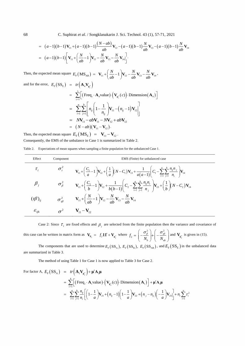
Then, the expected mean square F E 11 12MSE V V .
Consequently, the EMS of the unbalance in Case 1 is summarized in Table 2.
Table 2. Expectations of mean squares when sampling a finite population for the unbalanced Case 1.
Effect Component EMS (Finite) for unbalanced case
i
j
( )ij
ijk
2
2
2
2
111 12 1 13 1 14
1 1
1 11
1
a bij j
i j i
n nCN C C
a a a a n
V V V V
2
11 12 2 13 2 14
1 1
1 11
1
a bij i
i j j
n nCC N C
b b b n b
V V V V
11 12 13 141N N N
ab ab ab
V V V V
11 12V V
Case 2: Since i are fixed effects and
j are selected from the finite population then the variance and covariance of
this case can be written in matrix form as *
2 22f F F
V 11 V where
2 2
2
b ab
fN N
and *2F
V is given in (15).
The components that are used to determine F A F BSS , SS ,E E F ABSSE , and F ESSE in the unbalanced data
are summarized in Table 3.
The method of using Table 1 for Case 1 is now applied to Table 3 for Case 2.
For factor A, *2
F A 1 1SSE tr F
A V μ A μ
*2
4
1 1 1
1
Freq value ( ) Dimensionc
c
c
F
A V A μ A μ
2
21 22 23
1 1 1
1 1 11 1 1
a b aij
ij j ij i i
i j ii
nn n n n
n a a a
V V V
C. Suphirat et al. / Songklanakarin J. Sci. Technol. 43 (1), 57-71, 2021 69
2 2
2
21 22 23
1 1 1 1 1 1 1
1 11 1
a b a b a b aij ij j ij
i i
i j i j i j ii i i
n n n na a n
n a n n a
V V V
2121 22 1 23
1 1 1
11 1
1 1
a b aij j i
i
i j ii
n n nCa C
a a a n a
V V V .
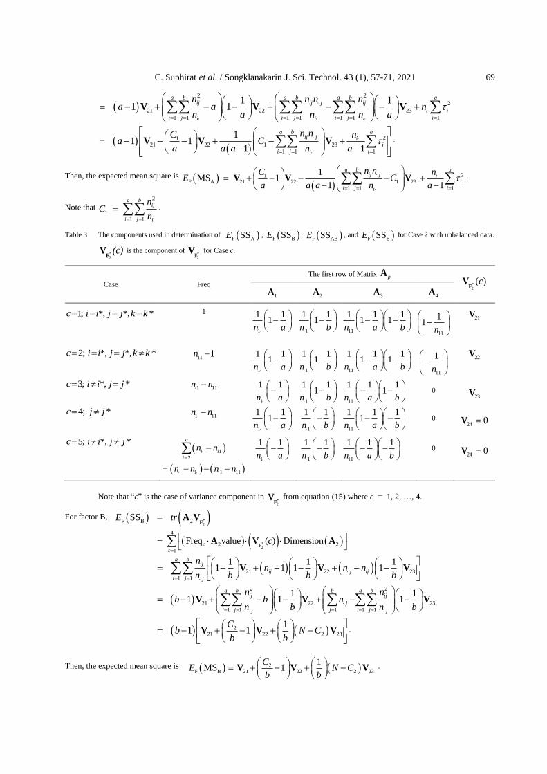
Then, the expected mean square is
21F A 21 22 1 23
1 1 1
1MS 1
1 1
a b aij j i
i
i j ii
n n nCE C
a a a n a
V V V .
Note that
2
1
1 1
a bij
i j i
nC
n
.
Table 3. The components used in determination of F ASSE , F BSSE , F ABSSE , and F ESSE for Case 2 with unbalanced data.
*2
(c)F
V is the component of *2F
V for Case c.
Case Freq
The first row of Matrix pA
*2
( )cF
V
1A 2A 3A 4A
1; *, *, *c i i j j k k 1
1
1 11
n a
1
1 11
n b
11
1 1 11 1
n a b
11
11
n
21V
2; *, *, *c i i j j k k
11 1n
1
1 11
n a
1
1 11
n b
11
1 1 11 1
n a b
11
1
n
22V
3; *, *c i i j j 1 11n n
1
1 1
n a
1
1 11
n b
11
1 1 11
n a b
0
23V
4; *c j j
1 11n n
1
1 11
n a
1
1 1
n b
11
1 1 11
n a b
0
24 0V
5; *, *c i i j j
1
2
1 1 11
a
i i
i
n n
n n n n
1
1 1
n a
1
1 1
n b
11
1 1 1
n a b
0
24 0V
Note that “c” is the case of variance component in 2*F
V from equation (15) where c = 1, 2, …, 4.
For factor B, *2
F B 2SSE trF
A V
*2
4
2 2
1
Freq value ( ) Dimensionc
c
c
F
A V A
21 22 23
1 1
1 1 11 1 1 1
a bij
ij j ij
i j j
nn n n
n b b b
V V V
2 2
21 22 23
1 1 1 1 1
1 11 1 1
a b b a bij ij
j
i j j i jj j
n nb b n
n b n b
V V V
221 22 2 23
11 1
Cb N C
b b
V V V .
Then, the expected mean square is 2F B 21 22 2 23
1MS 1
CE N C
b b
V V V .

70 C. Suphirat et al. / Songklanakarin J. Sci. Technol. 43 (1), 57-71, 2021
Note that:
1
b
j
j
N n
and
2
2
1 1
a bij
i j j
nC
n
.
For the AB interaction, *2
F AB 3SSE trF
A V
*2
4
3 3
1
Freq value ( ) Dimensionc
c
c
F
A V A
21 22 23
1 1
1 1 1 1 1 11 1 1 1 1 1
a b
ij j ij
i j
n n na b a b a b
V V V
21 22 23
1 1 1 1
1 1 1 11 1 1 1 1
a b a b
j ij
i j i j
a b N ab n na b a b
V V V
21 22 231 1 1N N
a bab ab
V V V .
Then, the expected mean square is F AB 21 22 23MS 1N N
Eab ab
V V V
and for the error, *2
F E 4SSE trF
A V
*2
4
4 4
1
Freq value ( ) Dimensionc
c
c
F
A V A
a b
ij 21 ij 22
i 1 j 1 ij
1n 1 n 1
n
V V
21 21 22 22N ab N ab V V V V
21 22N ab V V .
Then, the expected mean square is F E 21 22MSE V V .
Consequently, the EMS of the unbalanced in Case 2 is summarized in Table 4.
Table 4. Expectations of mean squares when sampling a finite population for the unbalanced Case 2.
Effect Component EMS (Finite) for unbalanced case
i
j
( )ij
ijk
2
1
1a
i
i
a
2
2
2
21
21 22 1 23
1 1 1
11
1 1
a b aij j i
i
i j ii
n n nCC
a a a n a
V V V
221 22 2 23
11
CN C
b b
V V V
21 22 231N N
ab ab
V V V
21 22V V
The EMS when sampling from a finite population
will be different from the EMS for an infinite population
( Sahai & Ojeda, 2004) . In particular, the multipliers of the
variance components for each model effect are not the same
when the random effects are sampled from a finite population.
4. Conclusions
In this research, we have determined the expected
mean squares for the random effects in the random and mixed
effects models in two-factor factorial model assuming finite
C. Suphirat et al. / Songklanakarin J. Sci. Technol. 43 (1), 57-71, 2021 71
populations for A, B, and AB interaction effects. The error,
however, is assumed to be 2N(0, ) .
For the case of balanced data, the expected mean
square formulas for factors A, B, and the AB interaction when
the random effects are sampled from finite populations are the
same as the infinite population case. However, the primary
differences are the values of the variance components. In the
infinite case, 2 , 2 , and 2
are assumed to follow nor-
mal distributions, while in the finite case they are the va-
riances of finite populations.
For an unbalanced case, the expected mean square
of error for finite population is equal to the expected mean
square for an infinite population. For the expected value of
mean square in factor A, B, and the AB interaction will not be
the same, because they depend on the multiplier values of the
population variances. Also, for the infinite case, 2 , 2 , and
2
are the variances of normally distributed random varia-
bles. For the finite case, they are the variances of finite popu-
lations.
Acknowledgements
The authors are thankful for the financial support by
the Department of Statistics, Faculty of Science, Kasetsart
University.
References
Clarke, B. R. (2008). Linear models: the theory and appli-
cation of analysis of variance. New Jersey, NJ: John
Wiley and Sons.
Cochran, W. G. (1977). Sampling techniques. New York, NY:
John Wiley and Sons.
Cornfield, J., & Tukey, J. W. (1956). Average values of mean
squares in factorials. The Annals of Mathematical
Statistics, 27(4), 907-949.
Gaylor, D. W., & Hartwell, T. D. (1969). Expected mean
squares for nested classifications. Biometrics, 427-
430.
Hartley, H. O. (1967). Expectations, variances and cova-
riances of ANOVA mean squares by synthe-
sis. Biometrics, 105-114.
Hocking, R. R. (1985). The analysis of linear models.
California, CA: Brooks/Cole Publishing.
Montgomery, D. C. (2013). Design and analysis of experi-
ments. New York, NJ: John Wiley and Sons.
Oehlert, G. W. (2010). A first course in design and analysis of
experiments. Retrieved from https://hdl.handle.net/
11299/168002.
Sahai, H., & Ojeda, M. M. (2003). Analysis of variance for
random models, Volume 1: Balanced data: Theory,
methods, applications, and data analysis. Berlin,
Germany: Springer Science and Business Media.
Sahai, H., & Ojeda, M. M. (2004). Analysis of variance for
random models, Volume 2: Unbalanced data:
Theory, methods, applications, and data analysis.
Berlin, Germany: Springer Science and Business
Media.
Searle, S. R., Casella, G., & McCulloch, C. E. (2009). Va-
riance components. New Jersey, NJ: John Wiley
and Sons.
Searle, S. R., & Fawcett, R. F. (1970). Expected mean squares
in variance components models having finite popu-
lations. Biometrics, 243-254.
Searle, S. R., & Henderson, C. R. (1961). Computing proce-
dures for estimating components of variance in the
two-way classification, mixed model. Biometrics, 17
(4), 607-616.
Simmachan, T., Borkowski, J. J., & Budsaba, K. (2012).
Expected mean squares for the random effects one-
way ANOVA model when sampling from a finite
population. Thailand Statistician, 10(1), 121-128.
Tukey, J. W. (1956). Variances of variance components: I.
Balanced designs. The Annals of Mathematical Sta-
tistics, 27(3), 722-736.
Tukey, J. W. (1957). Variances of variance components: II.
The unbalanced single classification. The Annals of
Mathematical Statistics, 28(1), 43-56.