expected mean squares fixed vs. random effects
TRANSCRIPT

1
EXPECTED MEAN SQUARES Fixed vs. Random Effects • The choice of labeling a factor as a fixed or random effect will affect how you will make the F-test.
• This will become more important later in the course when we discuss interactions. Fixed Effect • All treatments of interest are included in your experiment. • You cannot make inferences to a larger experiment. Example 1: An experiment is conducted at Fargo and Grand Forks, ND. If location is considered a fixed effect, you cannot make inferences toward a larger area (e.g. the central Red River Valley). Example 2: An experiment is conducted using four rates (e.g. ½ X, X, 1.5 X, 2 X) of a herbicide to determine its efficacy to control weeds. If rate is considered a fixed effect, you cannot make inferences about what may have occurred at any rates not used in the experiment (e.g. ¼ x, 1.25 X, etc.). Random Effect • Treatments are a sample of the population to which you can make inferences. • You can make inferences toward a larger population using the information from the analyses. Example 1: An experiment is conducted at Fargo and Grand Forks, ND. If location is considered a random effect, you can make inferences toward a larger area (e.g. you could use the results to state what might be expected to occur in the central Red River Valley). Example 2: An experiment is conducted using four rates (e.g. ½ X, X, 1.5 X, 2 X) of an herbicide to determine its efficacy to control weeds. If rate is considered a random effect, you can make inferences about what may have occurred at rates not used in the experiment (e.g. ¼ x, 1.25 X, etc.).

2
Why Do We Need To Learn How to Write Expected Mean Squares?
• So far in class we have assumed that treatments are always a fixed effect.
• If some or all factors in an experiment are considered random effects, we need to be concerned about the denominator of the F-test because it may not be the Error MS.
• To determine the appropriate denominator of the F-test, we need to know how to write
the Expected Mean Squares for all sources of variation. All Random Model Each source of variation will consist of a linear combination of 2σ plus variance components whose subscript matches at least one letter in the source of variation. The coefficients for the identified variance components will be the letters not found in the subscript of the variance components. Example – RCBD with a 3x4 Factorial Arrangement Sources of variation 2σ 2
ABrσ 2Braσ 2
Arbσ 2Rabσ
Rep 22Rabσσ +
A 222AAB rbr σσσ ++
B 222BAB rar σσσ ++
AxB 22ABrσσ +
Error 2σ Step 1. Write the list of variance components across the top of the table.
- There will be one variance component for each source of variation except Total. - The subscript for each variance component will correspond to each source of variation. - The variance component for error receives no subscript.
Sources of variation 2σ 2
ABσ 2Bσ 2
Aσ 2Rσ
Rep A B AxB Error
3
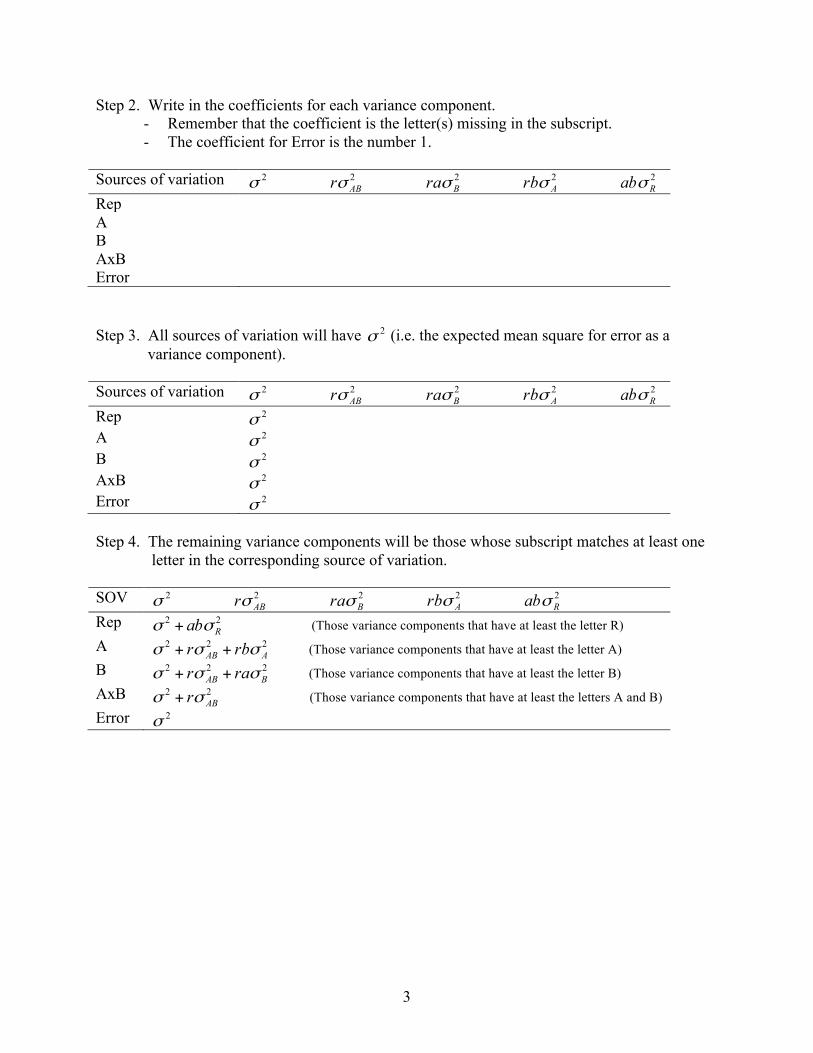
Step 2. Write in the coefficients for each variance component. - Remember that the coefficient is the letter(s) missing in the subscript. - The coefficient for Error is the number 1.
Sources of variation 2σ 2
ABrσ 2Braσ 2
Arbσ 2Rabσ
Rep A B AxB Error Step 3. All sources of variation will have 2σ (i.e. the expected mean square for error as a
variance component). Sources of variation 2σ 2
ABrσ 2Braσ 2
Arbσ 2Rabσ
Rep 2σ A 2σ B 2σ AxB 2σ Error 2σ Step 4. The remaining variance components will be those whose subscript matches at least one
letter in the corresponding source of variation.
SOV 2σ 2ABrσ 2
Braσ 2Arbσ 2
Rabσ Rep 22
Rabσσ + (Those variance components that have at least the letter R) A 222
AAB rbr σσσ ++ (Those variance components that have at least the letter A) B 222
BAB rar σσσ ++ (Those variance components that have at least the letter B) AxB 22
ABrσσ + (Those variance components that have at least the letters A and B) Error 2σ

4
Example – CRD with a 4x3x2 Factorial Arrangement Sources of variation 2σ 2
ABCrσ 2BCraσ 2
ACrbσ 2ABrcσ 2
Crabσ 2Bracσ 2
Arbcσ A 22222
AABACABC rbcrcrbr σσσσσ ++++ B 22222
BABBCABC racrcrar σσσσσ ++++ C 22222
CACBCABC rabrbrar σσσσσ ++++ AxB 222
ABABC rcr σσσ ++ AxC 222
ACABC rbr σσσ ++ BxC 222
BCABC rar σσσ ++ AxBxC 22
ABCrσσ + Error 2σ Step 1. Write the list of variance components across the top of the table.
- There will be one variance component for each source of variation except Total. - The subscript for each variance component will correspond to each source of variation. - The variance component for error receives no subscript.
Sources of variation 2σ 2ABCσ 2
BCσ 2ACσ 2
ABσ 2Cσ 2
Bσ 2Aσ
A B C AxB AxC BxC AxBxC Error

5
Step 2. Write in the coefficients for each variance component. - Remember that the coefficient is the letter(s) missing in the subscript. - The coefficient for Error is the number 1.
Sources of variation 2σ 2
ABCrσ 2BCraσ 2
ACrbσ 2ABrcσ 2
Crabσ 2Bracσ 2
Arbcσ A B C AxB AxC BxC AxBxC Error Step 3. All sources of variation will have 2σ (i.e. the expected mean square for error as a
variance component). Sources of variation 2σ 2
ABCrσ 2BCraσ 2
ACrbσ 2ABrcσ 2
Crabσ 2Bracσ 2
Arbcσ A 2σ B 2σ C 2σ AxB 2σ AxC 2σ BxC 2σ AxBxC 2σ Error 2σ Step 4. The remaining variance components will be those whose subscript matches at least one
letter in the corresponding source of variation. SOV 2σ 2
ABCrσ 2BCraσ 2
ACrbσ 2ABrcσ 2
Crabσ 2Bracσ 2
Arbcσ A 22222
AABACABC rbcrcrbr σσσσσ ++++ (Those variance components that have at least the letters A) B 22222
BABBCABC racrcrar σσσσσ ++++ (Those variance components that have at least the letter B) C 22222
CACBCABC rabrbrar σσσσσ ++++ (Those variance components that have at least the letter C) AxB 222
ABABC rcr σσσ ++ (Those variance components that have at least the letters A and B) AxC 222
ACABC rbr σσσ ++ (Those variance components that have at least the letters A and C) BxC 222
BCABC rar σσσ ++ (Those variance components that have at least the letters B and C) AxBxC 22
ABCrσσ + (Those variance components that have at least the letters A, B and C) Error 2σ
6
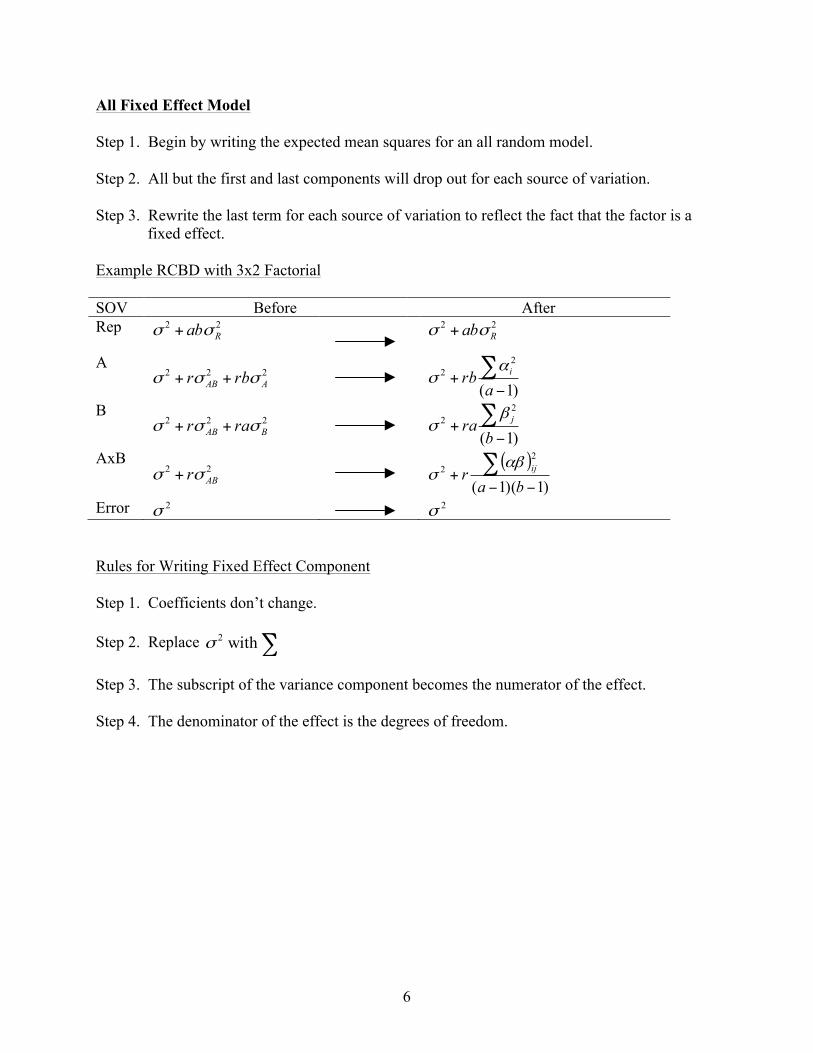
All Fixed Effect Model Step 1. Begin by writing the expected mean squares for an all random model. Step 2. All but the first and last components will drop out for each source of variation. Step 3. Rewrite the last term for each source of variation to reflect the fact that the factor is a fixed effect. Example RCBD with 3x2 Factorial SOV Before After Rep 22
Rabσσ + 22Rabσσ +
A 222AAB rbr σσσ ++
)1(
22
−+ ∑
arb iασ
B 222BAB rar σσσ ++
)1(
22
−+ ∑
bra jβσ
AxB 22ABrσσ +
( ))1)(1(
22
−−+ ∑
bar ijαβ
σ
Error 2σ 2σ Rules for Writing Fixed Effect Component Step 1. Coefficients don’t change. Step 2. Replace ∑ with 2σ Step 3. The subscript of the variance component becomes the numerator of the effect. Step 4. The denominator of the effect is the degrees of freedom.
7
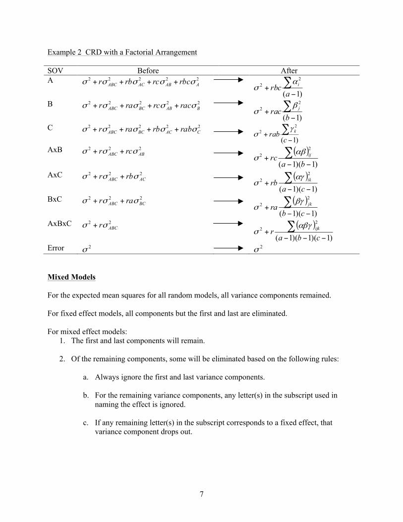
Example 2 CRD with a Factorial Arrangement SOV Before After A 22222
AABACABC rbcrcrbr σσσσσ ++++
)1(
22
−+ ∑
arbc iασ
B 22222BABBCABC racrcrar σσσσσ ++++
)1(
22
−+ ∑
brac jβσ
C 22222CACBCABC rabrbrar σσσσσ ++++
)1(
22
−+ ∑
crab kγσ
AxB 222ABABC rcr σσσ ++ ( )
)1)(1(
22
−−+ ∑
barc ijαβ
σ
AxC 222ACABC rbr σσσ ++ ( )
)1)(1(
22
−−+ ∑
carb ikαγ
σ
BxC 222BCABC rar σσσ ++ ( )
)1)(1(
22
−−+ ∑
cbra jkβγ
σ
AxBxC 22ABCrσσ + ( )
)1)(1)(1(
22
−−−+ ∑
cbar ijkαβγ
σ
Error 2σ 2σ Mixed Models For the expected mean squares for all random models, all variance components remained. For fixed effect models, all components but the first and last are eliminated. For mixed effect models:
1. The first and last components will remain. 2. Of the remaining components, some will be eliminated based on the following rules:
a. Always ignore the first and last variance components. b. For the remaining variance components, any letter(s) in the subscript used in
naming the effect is ignored.
c. If any remaining letter(s) in the subscript corresponds to a fixed effect, that variance component drops out.
8
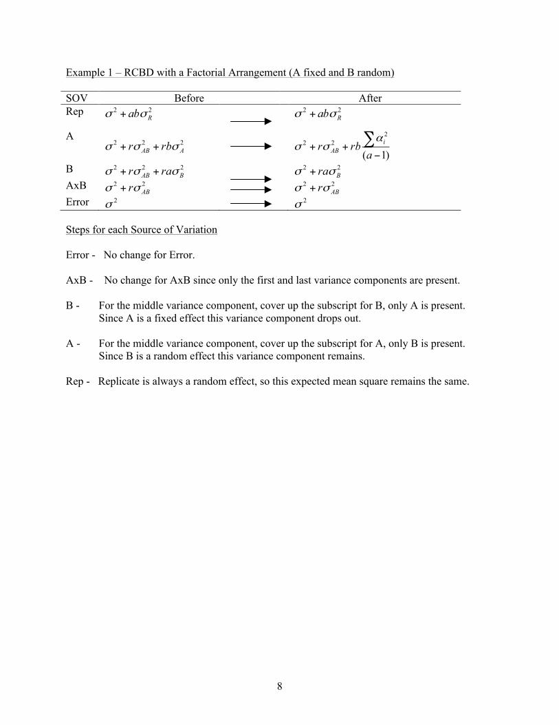
Example 1 – RCBD with a Factorial Arrangement (A fixed and B random) SOV Before After Rep 22
Rabσσ + 22Rabσσ +
A 222AAB rbr σσσ ++
)1(
222
−++ ∑
arbr i
AB
ασσ
B 222BAB rar σσσ ++ 22
Braσσ + AxB 22
ABrσσ + 22ABrσσ +
Error 2σ 2σ Steps for each Source of Variation Error - No change for Error. AxB - No change for AxB since only the first and last variance components are present. B - For the middle variance component, cover up the subscript for B, only A is present. Since A is a fixed effect this variance component drops out. A - For the middle variance component, cover up the subscript for A, only B is present.
Since B is a random effect this variance component remains. Rep - Replicate is always a random effect, so this expected mean square remains the same.

9
Example 2 CRD with a Factorial Arrangement (A fixed, B and C random) SOV Before After A 22222
AABACABC rbcrcrbr σσσσσ ++++
)1(
22222
−++++ ∑
arbcrcrbr i
ABACABC
ασσσσ
B 22222BABBCABC racrcrar σσσσσ ++++ 222
BBC racra σσσ ++ C 22222
CACBCABC rabrbrar σσσσσ ++++ 222CBC rabra σσσ ++
AxB 222ABABC rcr σσσ ++ 222
ABABC rcr σσσ ++ AxC 222
ACABC rbr σσσ ++ 222ACABC rbr σσσ ++
BxC 222BCABC rar σσσ ++ 22
BCraσσ + AxBxC 22
ABCrσσ + 22ABCrσσ +
Error 2σ 2σ Steps for Each Source of Variation Error - Error remains the same. AxBxC - The error mean square for AxBxC remains the same since there are only first and last terms. BxC - Cover up the B and C in the subscript, A remains and corresponds to a fixed effect.
Therefore the term drops out. AxC - Cover up the A and C in the subscript, B remains and corresponds to a random effect.
Therefore the term remains. AxB - Cover up the A and B in the subscript, C remains and corresponds to a random effect.
Therefore the term remains. C - ABC term - Cover up the C term in the subscript, A and B remain. A corresponds to a fixed effect and B corresponds to a random effect. Since one of the terms corresponds to a fixed effect, the variance component drops out. BC term - Cover up the C term in the subscript, B remains. B corresponds to a random effect. Since B is a random effect, the variance component remains. AC term - Cover up the C term in the subscript, A remains. A corresponds to a fixed effect. Since A is a fixed effect, the variance component drops out. B - ABC term - Cover up the B term in the subscript, A and C remain. A corresponds to a fixed effect and C corresponds to a random effect. Since one of the terms corresponds to a fixed effect, the variance component drops out.

10
BC term - Cover up the B term in the subscript, C remains. C corresponds to a random effect. Since B is a random effect, the variance component remains. AB term - Cover up the B term in the subscript, A remains. A corresponds to a fixed effect. Since A is a fixed effect, the variance component drops out. A - ABC term - Cover up the A term in the subscript, B and C remain. B and C correspond
to a random effect. Since none of the terms correspond to a fixed effect, the variance component remains.
AC term - Cover up the A term in the subscript, C remains. C corresponds to a random effect. Since C is a random effect, the variance component remains. AB term - Cover up the A term in the subscript, B remains. B corresponds to a random effect. Since B is a random effect, the variance component remains. Deciding What to Use as the Denominator of Your F-test For an all fixed model the Error MS is the denominator of all F-tests. For an all random or mix model,
1. Ignore the last component of the expected mean square. 2. Look for the expected mean square that now looks this expected mean square.
3. The mean square associated with this expected mean square will be the denominator of
the F-test.
4. If you can’t find an expected mean square that matches the one mentioned above, then you need to develop a Synthetic Error Term.
Example 1 – RCBD with a Factorial Arrangement (A fixed and B random) SOV Expected mean square MS F-test Rep 22
Rabσσ + 1 F = MS 1/MS 5
A
)1(
222
−++ ∑
arbr i
AB
ασσ 2 F = MS 2/MS 4
B 22Braσσ + 3 F = MS 3/MS 5
AxB 22ABrσσ + 4 F = MS 4/MS 5
Error 2σ 5
11
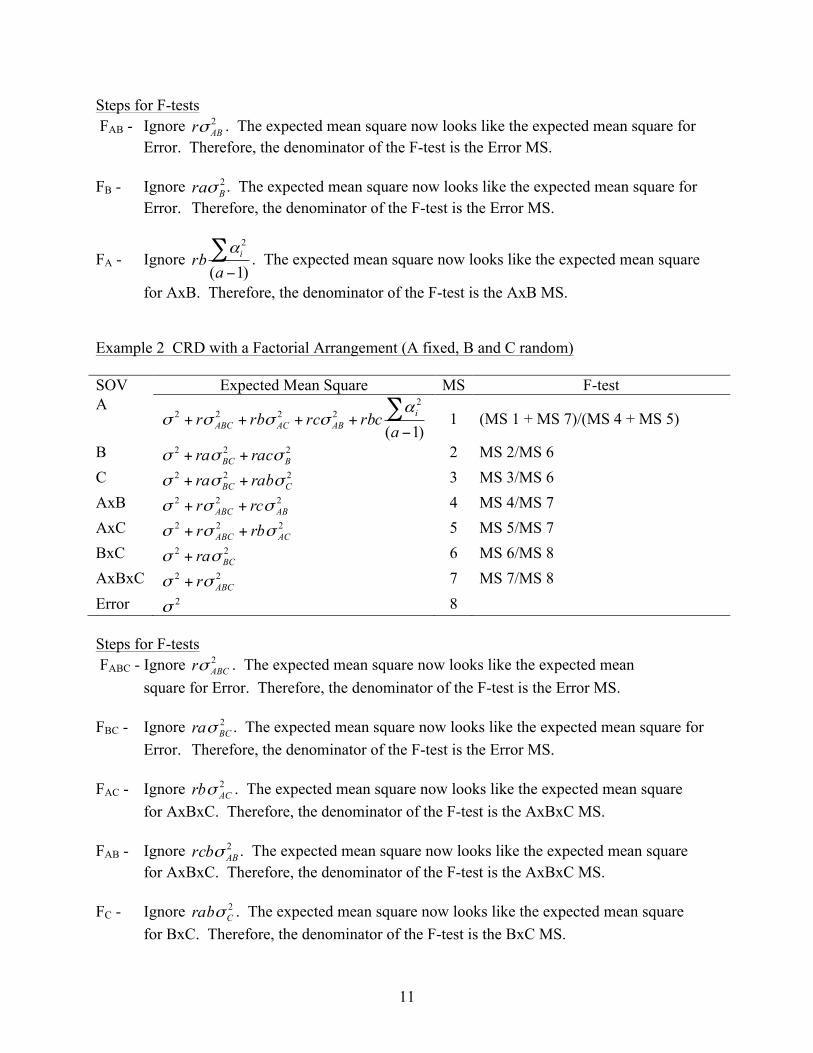
Steps for F-tests FAB - Ignore 2
ABrσ . The expected mean square now looks like the expected mean square for Error. Therefore, the denominator of the F-test is the Error MS. FB - Ignore 2
Braσ . The expected mean square now looks like the expected mean square for Error. Therefore, the denominator of the F-test is the Error MS.
FA - Ignore )1(
2
−∑a
rb iα . The expected mean square now looks like the expected mean square
for AxB. Therefore, the denominator of the F-test is the AxB MS. Example 2 CRD with a Factorial Arrangement (A fixed, B and C random) SOV Expected Mean Square MS F-test A
)1(
22222
−++++ ∑
arbcrcrbr i
ABACABC
ασσσσ 1 (MS 1 + MS 7)/(MS 4 + MS 5)
B 222BBC racra σσσ ++ 2 MS 2/MS 6
C 222CBC rabra σσσ ++ 3 MS 3/MS 6
AxB 222ABABC rcr σσσ ++ 4 MS 4/MS 7
AxC 222ACABC rbr σσσ ++ 5 MS 5/MS 7
BxC 22BCraσσ + 6 MS 6/MS 8
AxBxC 22ABCrσσ + 7 MS 7/MS 8
Error 2σ 8 Steps for F-tests FABC - Ignore 2
ABCrσ . The expected mean square now looks like the expected mean square for Error. Therefore, the denominator of the F-test is the Error MS. FBC - Ignore 2
BCraσ . The expected mean square now looks like the expected mean square for Error. Therefore, the denominator of the F-test is the Error MS. FAC - Ignore 2
ACrbσ . The expected mean square now looks like the expected mean square for AxBxC. Therefore, the denominator of the F-test is the AxBxC MS. FAB - Ignore 2
ABrcbσ . The expected mean square now looks like the expected mean square for AxBxC. Therefore, the denominator of the F-test is the AxBxC MS. FC - Ignore 2
Crabσ . The expected mean square now looks like the expected mean square for BxC. Therefore, the denominator of the F-test is the BxC MS.
12
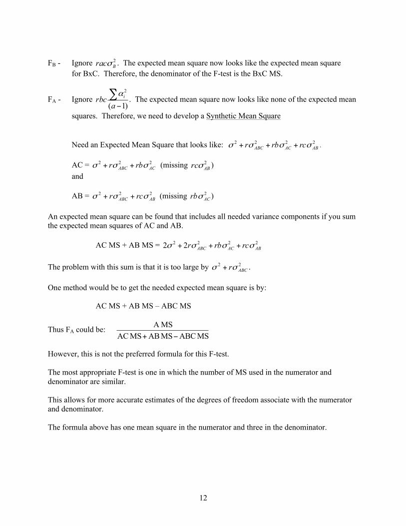
FB - Ignore 2
Bracσ . The expected mean square now looks like the expected mean square for BxC. Therefore, the denominator of the F-test is the BxC MS.
FA - Ignore )1(
2
−∑a
rbc iα . The expected mean square now looks like none of the expected mean
squares. Therefore, we need to develop a Synthetic Mean Square Need an Expected Mean Square that looks like: 2222
ABACABC rcrbr σσσσ +++ .
AC = 222ACABC rbr σσσ ++ (missing 2
ABrcσ ) and
AB = 222
ABABC rcr σσσ ++ (missing 2ACrbσ )
An expected mean square can be found that includes all needed variance components if you sum the expected mean squares of AC and AB.
AC MS + AB MS = 2222 22 ABACABC rcrbr σσσσ +++
The problem with this sum is that it is too large by 22
ABCrσσ + . One method would be to get the needed expected mean square is by:
AC MS + AB MS – ABC MS
Thus FA could be: MS ABCMS ABMS AC
MSA −+
However, this is not the preferred formula for this F-test. The most appropriate F-test is one in which the number of MS used in the numerator and denominator are similar. This allows for more accurate estimates of the degrees of freedom associate with the numerator and denominator. The formula above has one mean square in the numerator and three in the denominator.

13
The formula for FA that is most appropriate is
MS ABMS ACMS ABC MSA
++
The numerator and the denominator then become: 2222 22 ABACABC rcrbr σσσσ +++ . Calculation of Estimated Degrees of Freedom Calculation of degrees of freedom for the numerator and denominator of the F-test cannot be calculated by adding together the degrees of freedom for the associated mean squares.
For the F-test: FA = MS ABMS ACMS ABC MSA
++
The numerator degrees of freedom = ( )
⎥⎦
⎤⎢⎣
⎡+
+
df ABCMS) ABC(
dfA MS)A (
MS ABC MSA 22
2
The denominator degrees of freedom = ( )
⎥⎦
⎤⎢⎣
⎡+
+
df ABMS) AB(
df ACMS) AC(
MS AB MS AC22
2
Calculation of LSD Values – CRD with a Factorial Arrangement (A fixed, B and C Random)
LSDABC (0.05) = r
MS2Error t dfError 0.05/2;
LSDBC (0.05) = ra
MS2Error t dfError 0.05/2;
LSDAC (0.05) = rb
MS) 2(ABCt df ABC 0.05/2;
LSDAB (0.05) = rc
MS) 2(ABCt df ABC 0.05/2;
14
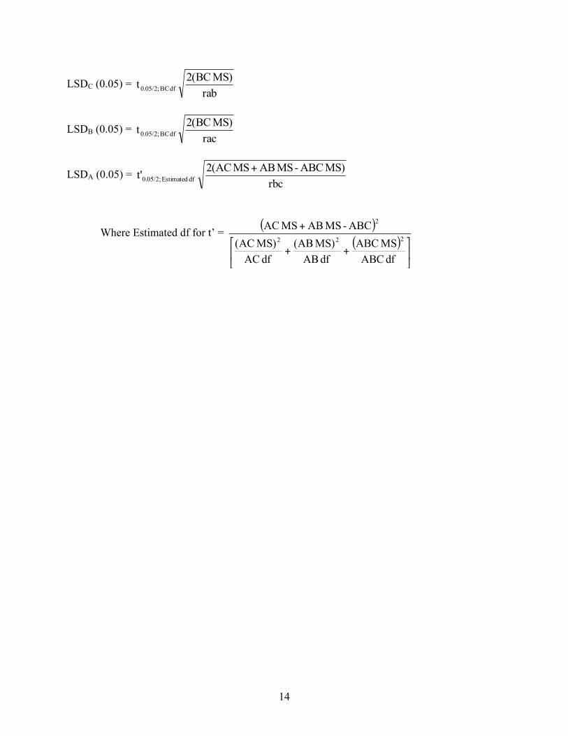
LSDC (0.05) = rab
MS) 2(BCt df BC 0.05/2;
LSDB (0.05) = rac
MS) 2(BCt df BC 0.05/2;
LSDA (0.05) = rbc
MS) ABC - MS AB MS 2(ACt' df Estimated 0.05/2;+
Where Estimated df for t’ = ( )( )
⎥⎦
⎤⎢⎣
⎡++
+
df ABCMS ABC
df ABMS) AB(
df ACMS) AC(
ABC - MS AB MS AC222
2
288
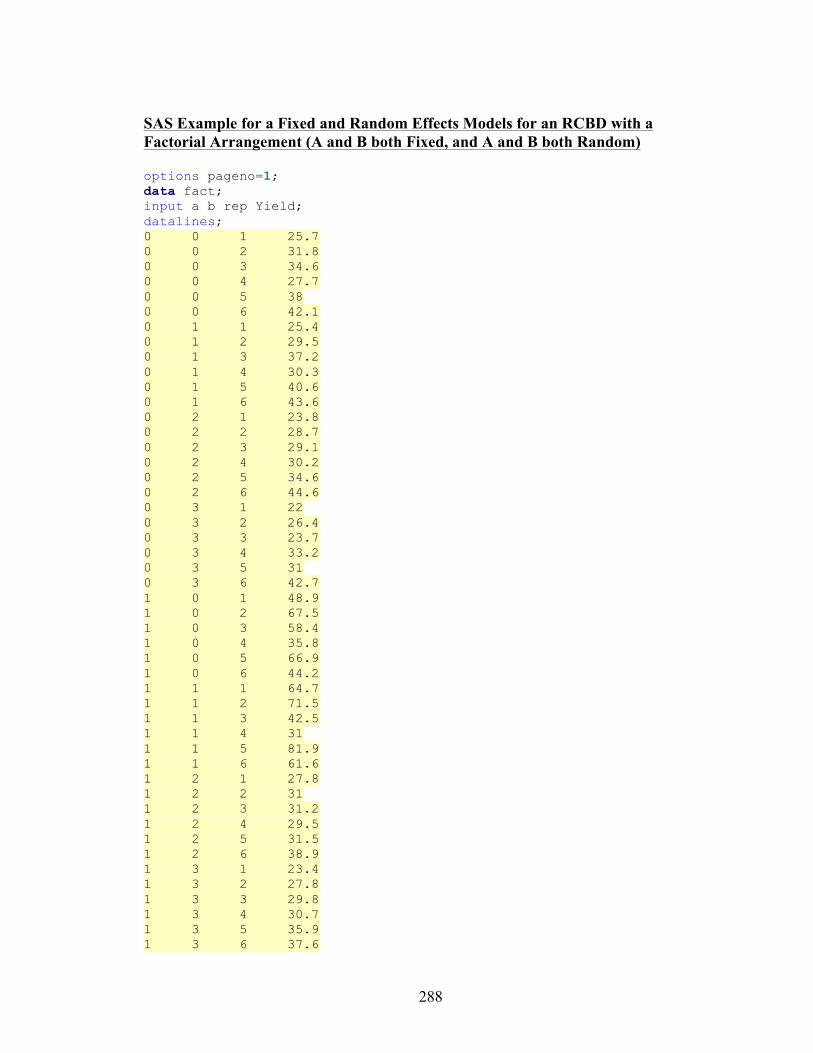
SAS Example for a Fixed and Random Effects Models for an RCBD with a Factorial Arrangement (A and B both Fixed, and A and B both Random) options pageno=1; data fact; input a b rep Yield; datalines; 0 0 1 25.7 0 0 2 31.8 0 0 3 34.6 0 0 4 27.7 0 0 5 38 0 0 6 42.1 0 1 1 25.4 0 1 2 29.5 0 1 3 37.2 0 1 4 30.3 0 1 5 40.6 0 1 6 43.6 0 2 1 23.8 0 2 2 28.7 0 2 3 29.1 0 2 4 30.2 0 2 5 34.6 0 2 6 44.6 0 3 1 22 0 3 2 26.4 0 3 3 23.7 0 3 4 33.2 0 3 5 31 0 3 6 42.7 1 0 1 48.9 1 0 2 67.5 1 0 3 58.4 1 0 4 35.8 1 0 5 66.9 1 0 6 44.2 1 1 1 64.7 1 1 2 71.5 1 1 3 42.5 1 1 4 31 1 1 5 81.9 1 1 6 61.6 1 2 1 27.8 1 2 2 31 1 2 3 31.2 1 2 4 29.5 1 2 5 31.5 1 2 6 38.9 1 3 1 23.4 1 3 2 27.8 1 3 3 29.8 1 3 4 30.7 1 3 5 35.9 1 3 6 37.6
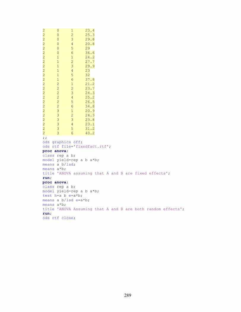
289
2 0 1 23.4 2 0 2 25.3 2 0 3 29.8 2 0 4 20.8 2 0 5 29 2 0 6 36.6 2 1 1 24.2 2 1 2 27.7 2 1 3 29.9 2 1 4 23 2 1 5 32 2 1 6 37.8 2 2 1 21.2 2 2 2 23.7 2 2 3 24.3 2 2 4 25.2 2 2 5 26.5 2 2 6 34.8 2 3 1 20.9 2 3 2 24.3 2 3 3 23.8 2 3 4 23.1 2 3 5 31.2 2 3 6 40.2 ;; ods graphics off; ods rtf file='fixedfact.rtf'; proc anova; class rep a b; model yield=rep a b a*b; means a b/lsd; means a*b; title 'ANOVA assuming that A and B are fixed effects'; run; proc anova; class rep a b; model yield=rep a b a*b; test h=a b e=a*b; means a b/lsd e=a*b; means a*b; title 'ANOVA Assuming that A and B are both random effects'; run; ods rtf close;
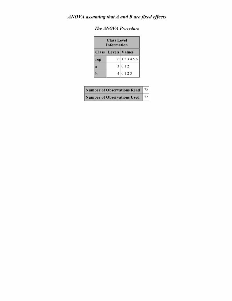
ANOVA assuming that A and B are fixed effects
The ANOVA Procedure
Class Level Information
Class Levels Values
rep 6 1 2 3 4 5 6
a 3 0 1 2
b 4 0 1 2 3
Number of Observations Read 72
Number of Observations Used 72
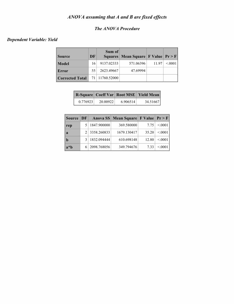
ANOVA assuming that A and B are fixed effects
The ANOVA Procedure Dependent Variable: Yield
Source DF Sum of
Squares Mean Square F Value Pr > F
Model 16 9137.02333 571.06396 11.97 <.0001
Error 55 2623.49667 47.69994
Corrected Total 71 11760.52000
R-Square Coeff Var Root MSE Yield Mean
0.776923 20.00922 6.906514 34.51667
Source DF Anova SS Mean Square F Value Pr > F
rep 5 1847.900000 369.580000 7.75 <.0001
a 2 3358.260833 1679.130417 35.20 <.0001
b 3 1832.094444 610.698148 12.80 <.0001
a*b 6 2098.768056 349.794676 7.33 <.0001

ANOVA assuming that A and B are fixed effects
The ANOVA Procedure
t Tests (LSD) for Yield
Note: This test controls the Type I comparisonwise error rate, not the experimentwise error rate.
Alpha 0.05
Error Degrees of Freedom 55
Error Mean Square 47.69994
Critical Value of t 2.00404
Least Significant Difference 3.9955
Means with the same letter are not significantly
different.
t Grouping Mean N a
A 43.750 24 1
B 32.354 24 0
C 27.446 24 2

ANOVA assuming that A and B are fixed effects
The ANOVA Procedure
t Tests (LSD) for Yield
Note: This test controls the Type I comparisonwise error rate, not the experimentwise error rate.
Alpha 0.05
Error Degrees of Freedom 55
Error Mean Square 47.69994
Critical Value of t 2.00404
Least Significant Difference 4.6137
Means with the same letter are not significantly
different.
t Grouping Mean N b
A 40.800 18 1
A
A 38.139 18 0
B 29.811 18 2
B
B 29.317 18 3
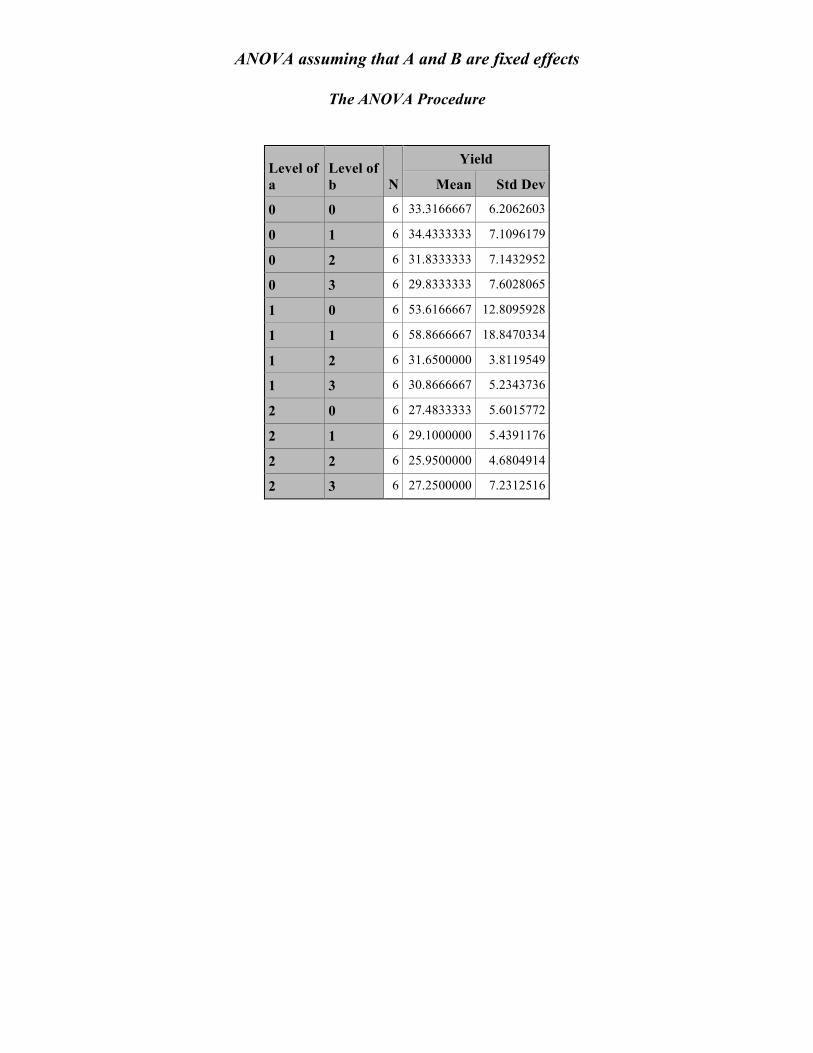
ANOVA assuming that A and B are fixed effects
The ANOVA Procedure
Level of a
Level of b N
Yield
Mean Std Dev
0 0 6 33.3166667 6.2062603
0 1 6 34.4333333 7.1096179
0 2 6 31.8333333 7.1432952
0 3 6 29.8333333 7.6028065
1 0 6 53.6166667 12.8095928
1 1 6 58.8666667 18.8470334
1 2 6 31.6500000 3.8119549
1 3 6 30.8666667 5.2343736
2 0 6 27.4833333 5.6015772
2 1 6 29.1000000 5.4391176
2 2 6 25.9500000 4.6804914
2 3 6 27.2500000 7.2312516
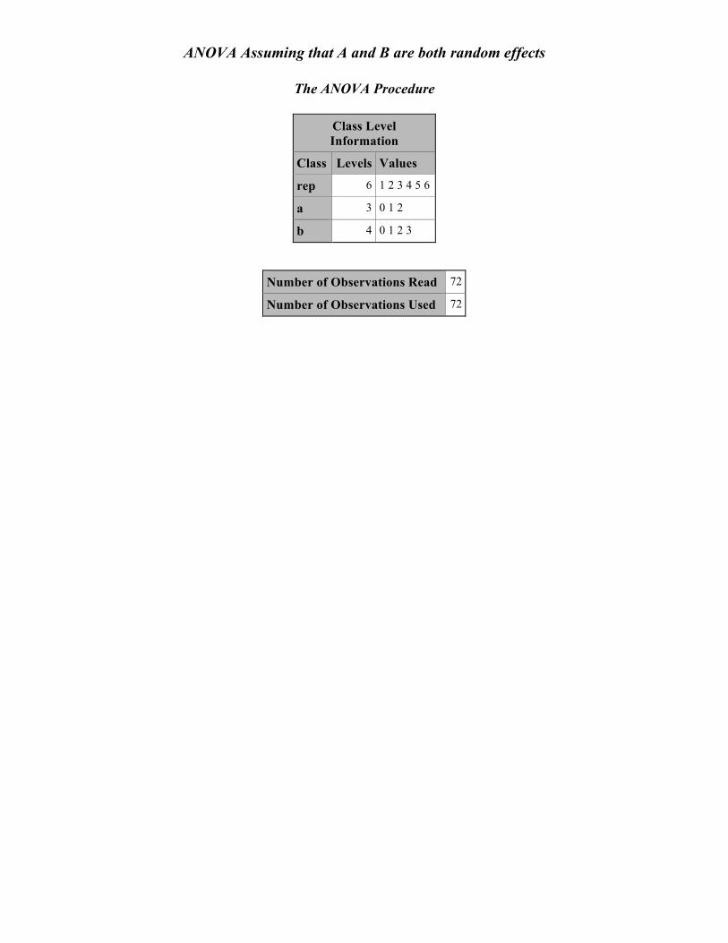
ANOVA Assuming that A and B are both random effects
The ANOVA Procedure
Class Level Information
Class Levels Values
rep 6 1 2 3 4 5 6
a 3 0 1 2
b 4 0 1 2 3
Number of Observations Read 72
Number of Observations Used 72

ANOVA Assuming that A and B are both random effects
The ANOVA Procedure Dependent Variable: Yield
Source DF Sum of
Squares Mean Square F Value Pr > F
Model 16 9137.02333 571.06396 11.97 <.0001
Error 55 2623.49667 47.69994
Corrected Total 71 11760.52000
R-Square Coeff Var Root MSE Yield Mean
0.776923 20.00922 6.906514 34.51667
Source DF Anova SS Mean Square F Value Pr > F
rep 5 1847.900000 369.580000 7.75 <.0001
a 2 3358.260833 1679.130417 35.20 <.0001
b 3 1832.094444 610.698148 12.80 <.0001
a*b 6 2098.768056 349.794676 7.33 <.0001
Tests of Hypotheses Using the Anova MS for a*b as an Error Term
Source DF Anova SS Mean Square F Value Pr > F
a 2 3358.260833 1679.130417 4.80 0.0569
b 3 1832.094444 610.698148 1.75 0.2569

ANOVA Assuming that A and B are both random effects
The ANOVA Procedure
t Tests (LSD) for Yield
Note: This test controls the Type I comparisonwise error rate, not the experimentwise error rate.
Alpha 0.05
Error Degrees of Freedom 6
Error Mean Square 349.7947
Critical Value of t 2.44691
Least Significant Difference 13.211
Means with the same letter are not significantly
different.
t Grouping Mean N a
A 43.750 24 1
A
B A 32.354 24 0
B
B 27.446 24 2
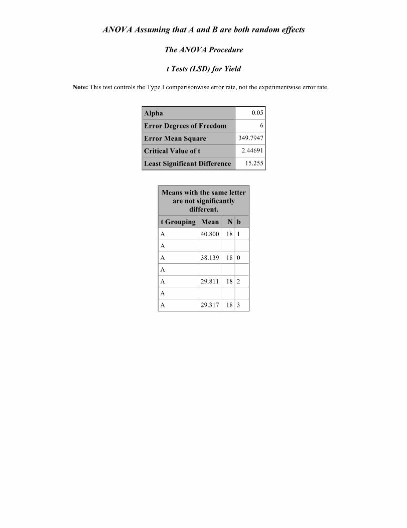
ANOVA Assuming that A and B are both random effects
The ANOVA Procedure
t Tests (LSD) for Yield
Note: This test controls the Type I comparisonwise error rate, not the experimentwise error rate.
Alpha 0.05
Error Degrees of Freedom 6
Error Mean Square 349.7947
Critical Value of t 2.44691
Least Significant Difference 15.255
Means with the same letter are not significantly
different.
t Grouping Mean N b
A 40.800 18 1
A
A 38.139 18 0
A
A 29.811 18 2
A
A 29.317 18 3

ANOVA Assuming that A and B are both random effects
The ANOVA Procedure
t Tests (LSD) for Yield
Level of a
Level of b N
Yield
Mean Std Dev
0 0 6 33.3166667 6.2062603
0 1 6 34.4333333 7.1096179
0 2 6 31.8333333 7.1432952
0 3 6 29.8333333 7.6028065
1 0 6 53.6166667 12.8095928
1 1 6 58.8666667 18.8470334
1 2 6 31.6500000 3.8119549
1 3 6 30.8666667 5.2343736
2 0 6 27.4833333 5.6015772
2 1 6 29.1000000 5.4391176
2 2 6 25.9500000 4.6804914
2 3 6 27.2500000 7.2312516