exchange rate volatility and the mixture of distribution hypothesis

DOI 10.1007/s00181-005-0005-x

ORIGINAL ARTICLE

Luc Bauwens . Dagfinn Rime . Genaro Sucarrat

Exchange rate volatility and the mixtureof distribution hypothesis

Published online: 26 October 2005© Springer-Verlag 2005

Abstract This study sheds new light on the mixture of distribution hypothesis bymeans of a study of the weekly exchange rate volatility of the Norwegian krone. Inline with other studies we find that the impact of information arrival on exchangerate volatility is positive and statistically significant, and that the hypothesis that anincrease in the number of traders reduces exchange rate volatility is not supported.The novelties of our study consist in documenting that the positive impact ofinformation arrival on volatility is relatively stable across three different exchangerate regimes, and in that the impact is relatively similar for both weekly volatilityand weekly realised volatility. It is not given that the former should be the casesince exchange rate stabilisation was actively pursued by the central bank in partsof the study period. We also report a case in which undesirable residual propertiesattained within traditional frameworks are easily removed by applying the log-transformation on volatilities.

Keywords Exchange rate volatility . Mixture of distribution hypothesis

JEL Classification F31

1 Introduction

If exchange rates walk randomly and if the number of steps depends positively onthe number of information events, then exchange rate volatility over a given period

L. Bauwens . G. Sucarrat (*)CORE and Department of Economics, Université catholique de Louvain,Louvain-la-Nueve, BelgiumE-mail: [email protected], [email protected],URL: http://www.core.ucl.ac.be/˜sucarrat/index.html

D. RimeNorges Bank, Oslo, NorwayE-mail: [email protected]

Empirical Economics 30:889–911 (2006)

should increase with the number of information events in that period. This chain ofreasoning is the essence of the so-called “mixture of distribution hypothesis”(MDH) associated with Clark (1973) and others. Several versions of the MDH havebeen put forward, including one that suggests the size of the steps dependsnegatively on the number of traders, see for example Tauchen and Pitts (1983). Inother words, an increase in the number of traders, a measure of liquidity, shoulddecrease the size of the steps and thus volatility. Exchange rate volatility may ofcourse depend on other factors too, including country-specific institutional factors,market conditions and economic fundamentals. Bringing such factors together in ageneral framework and trying to disentangle their distinct effects on exchange ratevolatility leads to economic or explanatory volatility modelling as opposed to“pure” forecast modelling, which may remain silent about the economic reasons forvariation in volatility.

When Karpoff (1987) surveyed the relationship between financial volatility andtrading volume (a measure of information intensity) during the mid-eighties, onlyone out of the 19 studies he cited was on exchange rates. The increased availabilityof data brought by the nineties has changed this, and currently we are aware of tenstudies that directly or indirectly investigate the relationship between exchange ratevolatility and information intensity. The ten studies are summarised in Table 1 andour study of Norwegian weekly exchange rate volatility from 1993 to 2003 adds tothis literature in several ways. First, our study spans more than a decade coveringthree different exchange rate regimes. Second, not only do we find that the impactof changes in the number of information events on exchange rate volatility ispositive and statistically significant, recursive parameter analysis suggests theimpact is relatively stable across the different exchange rate regimes. Finally, ourresults do not support the hypothesis that an increase in the number of tradersreduces exchange rate volatility.

Another contribution of our study concerns the economic modelling of ex-change rate volatility as such. We report a case in which undesirable residualproperties are easily removed by applying the logarithmic transformation onvolatilities. In particular, we show that OLS-regressions of the logarithm of vol-atility on its own lags and on several economic variables can produce uncorrelatedand homoscedastic residuals. Moreover, in the log of realised volatility case theresiduals are also normal. When Geweke (1986), Pantula (1986) and Nelson (1991)proposed that volatilities should be analysed in logs it was first and foremost inorder to ensure non-negativity. In our case the motivation stems from unsatis-factory residual properties and fragile inference results. Without the log-trans-formation we do not generally produce uncorrelated residuals, and when we do theresults are very sensitive to small changes in specification.

The rest of this paper contains three sections. In Section 2, we review the linkbetween exchange rate volatility and the MDH hypothesis, and discuss mea-surement issues. We also present our data and other economic variables that webelieve may impact on the volatility of the Norwegian exchange rate. In Section 3,we present the models we use and the empirical results. We conclude in thelast section, whereas an Appendix provides the details of the data sources andtransformations.

890 L. Bauwens et al.

2 Exchange rate volatility and economic determinants

The purpose of this section is to motivate and describe our exchange rate volatilitymeasures, and the economic determinants that we use in our empirical study. InSubsection 2.1, we define our volatility measures and present the Norwegianexchange rate data. We make a distinction between period volatility on the onehand and within or intra-period volatility on the other, arguing that analysis of bothis desirable since level-expectations may have an impact. In Subsection 2.2, wereview the link between volatility and the MDH, and after presenting our quotefrequency data we explain how we use them to construct the explanatory variableswe include in our volatility equations. In Subsection 2.3, we motivate and describethe other economic determinants of volatility which we include as explanatoryvariables in the empirical part.

2.1 Period vs. intra-period volatility measures

Conceptually we may distinguish between period volatility on the one hand andwithin or intra-period volatility on the other. If {S0,S1,...,Sn,..., SN−1,SN} denotes asequence of exchange rates between two currencies at times {0,1,...,N}, then thesquared (period) return [log(SN/S0)]

2 is an example of a period measure of observ-

Table 1 Summary of empirical studies that investigate the impact of information intensity onexchange rate volatility

Publication Data Period Supportiveof MDH?

Grammatikos andSaunders (1986)

Daily currency futures contracts (DEM, CHF,GBP, CAD and JPY) denominated in USD

1978–1983 Yes

Goodhart (1991) Intradaily quotes (USD against GBP, DEM,CHF, JPY, FRF, NLG, ITL, ECU) and Reuters’news-headline page

14/9–15/91987

No

Goodhart (2000) Intradaily quotes (USD against GBP, DEM, JPY,FRF, AUD) and Reuters’ news-headline pages

9/4-19/61989

No

Bollerslev andDomowitz (1993)

Intradaily USD/DEM quotes and quotingfrequency

9/4–30/61989

No

Demos andGoodhart (1996)

Intradaily DEM/USD and JPY/USD quotesand quoting frequency

5 weeks in1989

Yes

Jorion (1996) Daily DEM/USD futures and options Jan. 1985–Feb. 1992

Yes

Melvin and Xixi(2000)

Intradaily DEM/USD and JPY/USD quotes,quoting frequency and Reuters’ headline-newsscreen

1/12 1993–26/4 1995

Yes

Galati (2003) Daily quotes (USD against JPY and sevenemerging market currencies) and trading volume

1/1 1998–30/6 1999

Yes

Bauwens et al.(2005)

Intradaily EUR/USD quotes, quoting frequencyand Reuters’ news-alert screens

15/5 2001–14/11 2001

Yes

Bjønnes et al.(2005)

Daily SEK/EUR quotes and transaction volume 1995–2002 Yes

Exchange rate volatility and the mixture of distribution hypothesis 891

able volatility, and realised volatilityPN

n¼1 log Sn=Sn�1ð Þ½ �2 is an example of awithin-period measure of volatility. (Another example of a within-period measureof volatility is high–low.) It has been showed that realised volatility is an unbiasedand consistent measure of integrated volatility under certain assumptions, seeAndersen et al. (2001). The reader should be aware though that nowhere do we relyon such assumptions. Rather, our focus is on the formula of realised volatility. Themain difference between period volatility and realised volatility is that in additionto time 0 to time N variation the latter is also capable of capturing variation between0 and N. For example, if Sn fluctuates considerably between 0 and N but ends upclose to S0 at N, then the two measures may produce substantially different results.Essentially this can be due to one of two reasons. If the random walk modelprovides a decent description of how exchange rates behave, then it is due tochance. On the other hand, if there are strong level-effects present among marketparticipants, then the return back to the level of S0 might be due to market ex-pectations rather than chance. Although market participants’ views on exchangerate level clearly matter, we believe most observers would agree that such level-effects are relatively small or infrequent on a day-to-day basis for most exchangerates. Differently put, at very short horizons the random walk model provides areasonably good description of exchange rate increments. However, the two mea-sures are still qualitatively different, so that any eventual differences in theirrelation with (say) the rate of information arrival should be investigated, inparticular for weekly data where level-expectations is more likely to play a role.

Our period measure will be referred to as “weekly volatility” whereas ourwithin-period measure will be referred to as “within-weekly volatility” or “realisedvolatility.”Weekly volatility is just the squared return from the end of one week tothe end of the subsequent week. More precisely, if SN(t) denotes the closing value inthe last day of trading in week t and SN(t−1) denotes the closing value in the last dayof trading in the previous week, then weekly volatility recorded in week t isdenoted by Vt

w and defined as

Vwt ¼ log SN tð Þ

�SN t�1ð Þ

� �� 2: (1)

On the other hand, realised volatility in week t, denoted by Vtr, is the sum of

squared returns of the sequence {SN(t−1), S1(t), S2(t),.., SN(t)}, that is,

Vrt ¼

XN tð Þ

n¼1 tð Þlog Sn=Sn�1ð Þ½ �2; (2)

where 1(t)−1≔N(t−1). It should be noted though that we use only a small sub-set ofthe within-week observations in the construction of realised volatility (typically tenobservations per week).

In order to distinguish between volatilities and logs of volatilities we use lowerand upper case letters. So vt

w=log Vwt and vt

r=log Vtr. Our data set span the period

from 8 January 1993 to 26 December 2003, a total of 573 observations, and before1 January 1999 we use the BID NOK/DEM exchange rate converted to euro-equivalents with the official conversion rate 1.95583 DEM=1 EURO. After 1January 1999 we use the BID NOK/EUR rate.


The main characteristics of the two measures are contained in Table 2 and inFig. 1. At least three attributes of the graphs should be noted. First, although thetwo measures of volatility are similar level-wise, that is, if plotted in the samediagram they would be “on top of each other,” the sample correlation between thelog of weekly volatility and the log of realised volatility is only 0.55. In otherwords, the two measures differ considerably and one of the differences is that therealised volatility measure is less variable. Second, sustained increases in volatilityaround 1 January 1999 and 29 March 2001 are absent or at least seemingly so. Onthe first date the current central bank governor assumed the job and reinterpretedthe guidelines, which in practice entailed a switch from exchange rate stabilisationto “partial” inflation targeting. On the second date the Norwegian central bank wasinstructed by the Ministry of Finance to pursue an inflation target of 2.5% as mainpolicy objective. One might have expected that both of these changes would haveresulted in shifts upwards in volatility. However, if this is the case then this is notevident by just looking at the graphs. Alternatively, the apparent absence of shiftsin volatility might be due to the fact that the markets had expected these changesand already adapted to them. A third interesting feature is that there is a marked andlasting increase in volatility around late 1996 or in the beginning of 1997. This ispartly in line with Giot (2003) whose study supports the view that the Asian crisisin the second half of 1997 brought about a sustained increase in the volatility offinancial markets in general. In the case of Norwegian exchange rate volatility,however, the shift upwards seems to have taken place earlier, namely towards theend of 1996 or in the beginning of 1997. This may be attributed to the appreciatorypressure on the Norwegian krone in late 1996 and early 1997.

Table 2 Descriptive statistics of selected variables

St Δ st ∣Δ st∣ Vtw vt

w Vtr vt

r qt

Mean 8.208 0.000 0.005 0.578 −2.489 0.488 −1.659 7.5115Median 8.224 0.000 0.003 0.120 −2.121 0.209 −1.567 7.5192Max. 9.063 0.044 0.044 19.365 2.963 16.033 2.775 9.1363Min. 7.244 −0.035 0.000 0.000 −10.757 0.004 −5.497 5.6131St. dev. 0.352 0.008 0.006 1.679 2.447 1.035 1.413 0.5739Skew. 0.025 0.774 2.886 7.036 −0.845 8.418 −0.102 −0.3287Kurt. 2.174 9.399 14.991 65.150 3.884 107.193 2.793 3.4512Obs. 573 572 572 573 573 573 573 573

Δ qt ∣Δ qt∣ Mt Δ mt ∣Δ mt∣ mtw ft

a ftb

Mean 0.004 0.226 1.115 0.000 0.011 −0.556 0.007 0.010Median −0.003 0.145 1.124 −0.001 0.009 −0.190 0.000 0.000Max. 2.141 2.141 1.429 0.047 0.053 3.325 0.500 1.000Min. −1.278 0.000 0.838 −0.053 0.000 −9.150 0.000 0.000St.dev. 0.339 0.252 0.150 0.014 0.009 2.018 0.057 0.081Skew. 0.530 2.722 0.025 0.099 1.228 −1.015 8.271 9.136Kurt. 9.008 14.119 2.174 3.377 5.023 4.181 70.632 94.602Obs. 572 572 573 572 572 573 573 573

Some zero-values are due to rounding, and the variables are explained in Subsection 2.3 and inthe Appendix


2.2 MDH and quote frequency

If exchange rates follow a random walk and if the number of steps dependspositively on the number of information events, then exchange rate volatility over agiven period should increase with the number of information events in that period.This chain of reasoning is the essence of the MDH, an acronym which is due to the

Fig. 1 Weekly and realised NOK/EUR volatilities from 8 January 1993 to 26 December 2003(NOK/DEM before 1 January 1999) in the upper graph, log of weekly and realised volatilities inthe middle graph, and a scatter plot of the log-volatilities


statistical setup used by Clark (1973). Formally, focusing on the economic contentof the hypothesis, the MDH can also be formulated as

�st ¼XN tð Þ

n¼1

�sn; n ¼ 1; . . . ;N tð Þ; s0 ¼ sN t�1ð Þ; (3)

�snf gIID; �sn � N 0; 1ð Þ; (4)

@E N tð Þ �tj½ �@�t

> 0: (5)

where st=log St. The first line Eq. (3) states that the price increment of period t isequal to the sum of the intra-period increments, Eq. (4) is a random walkhypothesis (any “random walk” hypothesis would do), and Eq. (5) states that themean of the number of intra-period increments N(t) conditioned on the number ofinformation events vt in period t is strictly increasing in νt. Several variations of theMDH have been formulated, but for our purposes it is the economic content ofTauchen and Pitts (1983) that is of most relevance. In a nutshell, they argue that anincrease in the number of traders reduces the size of the intra-period increments.Here this is akin to replacing Eq. (4) with (say)

�sn ¼ �n �nð Þzn; �0n < 0; znf gIID; zn � N 0; 1ð Þ; (6)

where ηn denotes the number of traders at time n and where σ0n is the derivative. Butmarkets differ and theoretical models thus have to be adjusted accordingly. Inparticular, in a comparatively small currency market like the Norwegian anincrease in the number of currency traders is also likely to increase substantially thenumber of increments per period, that is, N(t), resulting in two counteractingeffects. One effect would tend to reduce period-volatility through the negativeimpact on the size of the intra-period increments, whereas the other effect wouldtend to increase period-volatility by increasing the number of increments. So it isnot known beforehand what the overall effect will be. Replacing Eq. (5) with

@E N tð Þ �t;j �t½ �@�t

> 0;@E N tð Þ �t;j �t½ �

@�t> 0; (7)

means the conditional mean of the number of increments N(t) is strictly increasingin both the number of information events νt and the number of traders ηt. TakingEq. (7) together with Eqs. (3) and (6) as our starting point we may formulate ournull hypotheses as

@Var �st �t�tjð Þ@�t

> 0 (8)

@Var �st �t; �tjð Þ@�t

< 0: (9)

In words, the first hypothesis states that an increase in the number ofinformation events given the number of traders increases period volatility, whereas


the second holds that an increase in the number of traders without changes in theinformation intensity reduces volatility. That Eq. (8) is the case is generallysuggested by Table 1, whereas Eq. (9) is suggested by Tauchen and Pitts (1983).However, it should be noted that the empirical results of Jorion (1996) and Bjønneset al. (2005) do not support the hypothesis that an increase in the number of tradersreduces volatility.

The most commonly used indicators of information arrival are selected samplesfrom the news-screens of Reuters or Telerate, quoting frequency, the number oftransacted contracts and transaction volume. The former is laborious to constructand at any rate not exhaustive with respect to the range of information events thatmight induce price revision, and the latter two are not readily available in foreignexchange markets. So quote frequency is our indicator of information arrival. Moreprecisely, before 1 January 1999 our quote series consists of the number of BIDNOK/DEM quotes per week, and after 1 January 1999 it consists of the number ofBID NOK/EUR quotes per week. We denote the log of the number of quotes inweek t by qt, but it should be noted that we have adjusted the series for two changesin the underlying data collection methodology, see the data Appendix for details.Graphs of qt and Δqt are contained in Fig. 2. In empirical analysis it is commonto distinguish between “expected” and “unexpected” activity, see amongst othersBessembinder and Seguin (1992), Jorion (1996) and Bjønnes et al. (2005). Ex-pected activity is supposed to reflect “normal” or “everyday” quoting or tradingactivity by traders, and should thus be negatively associated with volatilityaccording to Eq. (9) since this essentially reflects the number of active traders.Unexpected activity on the other hand refers to changes in the rate at which relevantinformation arrives to the market and should increase volatility. The strategy that isused in order to obtain the expected and unexpected components is to interpret thefitted values of an ARMA–GARCH model as the expected component and theresidual as the unexpected. In our case an ARMA(1,1) specification of Δqt with aGARCH(1,1) structure on the error terms suffices in order to obtain uncorrelatedstandardised residuals and uncorrelated squared standardised residuals. The modeland estimation output is contained in Table 3. The expected values are thencomputed by generating fitted values of qt (not of Δqt) and are denoted bqt . Theunexpected values are defined as qt � bqt . It has been argued that such a strategymight result in a so-called “generated regressor bias”-see for example Pagan(1984), so we opt for an alternative strategy which yields virtually identical results.As it turns out using qt directly instead of bqt , and Δqt instead of the residual, hasvirtually no effect on the estimates in Section 3. The reason can be deduced bylooking at the bottom graph of Fig. 2. For statistical purposes qt is virtuallyidentical to bqt , andΔqt is virtually identical to the residual (the sample correlationsare 0.85 and 0.94, respectively). Summarised, then, we use qt as our measure of thenumber of active traders and Δqt as our measure of changes in the rate at whichinformation arrives to the market. Both variables serve as explanatory variables inthe modelling of volatility in Section 3.

2.3 Other impact variables

Other economic variables may also influence the level of volatility and should becontrolled for in empirical models. In line with the conventions introduced above


lower-case means the log-transformation is applied, and upper-case means it is not.The only exceptions are the interest-rate variables, a Russian moratorium dummyidt equal to 1 in one of the weeks following the Russian moratorium (the weekcontaining Friday 28 August 1998 to be more precise) and 0 elsewhere, and a stepdummy sdt equal to 0 before 1997 and 1 after.

Fig. 2 The log of weekly number of BID NOK/EUR quotes (BID NOK/DEM before 1999) in theupper graph, the log-difference of weekly quoting in the middle graph, and scatter plots of qt vs.bqt and Δqt vs. residual in the bottom graph


The first economic variable is a measure of general currency market turbulenceand is measured through EUR/USD-volatility. If mt=log (EUR/USD)t, then Δmt

denotes the weekly return of EUR/USD, Mtw stands for weekly volatility, mt

w is itslog-counterpart, Mt

r is realised volatility and mtr is its log-counterpart. The pe-

troleum sector plays a major role in the Norwegian economy, so it makes sense toalso include a measure of oilprice volatility. If the log of the oilprice is denoted ot,then the weekly return isΔot, weekly volatility isOt

wwith otw as its log-counterpart,

and realised volatilities are denoted Otr and ot

r, respectively. We proceed similarlyfor the Norwegian and US stock market variables. If xt denotes the log of the mainindex of the Oslo stock exchange, then the associated variables areΔxt, Xt

w, xtw, Xt

r

and xtr. In the US case ut is the log of the New York stock exchange (NYSE) index

and the associated variables are Δut, Utw, ut

w, Utr and ut

r.The interest-rate variables that are included are constructed using the main

policy interest rate variable of the Norwegian central bank. We do not use marketinterest-rates because this produces interest-rate based measures that are sub-stantially intercorrelated with qt and sdt, with the consequence that inference resultsare affected. The interest-rate variables reflect two important regime changes thattook place over the period in question. As the current central bank governorassumed the position in 1999, the bank switched from exchange rate stabilisation to“partial” inflation targeting. However, a full mandate to target inflation was notgiven before 29 march 2001, when the Ministry of Finance instructed the bank totarget an inflation of 2.5%. So an interesting question is whether policy interest ratechanges contributed differently to exchange rate volatility in the partial and fullinflation targeting periods, respectively.1 This motivates the construction of ourinterest rate variables. Let Ft denote the main policy interest rate in percentages and

Table 3 ARMA–GARCH model of Δ qt :�qt ¼ b0 þ b1�qt�1 þ b2et�1 þ et;

et ¼ �tzt; �2t ¼ �0 þ �1e2t�1 þ �1�

2t�1

Parameter Diagnostics

Est. Pval. Est. Pval.

b0 0.004 0.13 R2 0.19b1 0.569 0.00 Log L -103.27b2 −0.910 0.00 Q(10) 11.03 0.20α0 0.034 0.02 ARCH1−10 0.29 0.98α1 0.299 0.00 JB 691.45 0.00β1 0.368 0.06 Obs. 571

Computations are in EViews 5.1 and estimates are ML with heteroscedasticity consistent standarderrors of the Bollerslev and Wooldridge (1992) type. Pval stands for p-value and corresponds to atwo-sided test with zero as null, Log L stands for log-likelihood, AR1−10 is the Ljung and Box(1979) test for serial correlation in the standardised residuals up to lag 10, ARCH1−10 is theF-form of the Lagrange-mulitplier test for serial correlation in the squared standardised residualsup to lag 10, Skew. is the skewness of the standardised residuals, Kurt. is the kurtosis of thestandardised residuals, and JB is the Jarque and Bera (1980) test for non-normality of thestandardised residuals

1 Prior to 1999 central bank interest rates were very stable, at least from late 1993 until late 1996,and it was less clear to the market what role the interest rate actually had.


let ΔFt denote the change from the end of 1 week to the end of the next.Furthermore, let Ia denote an indicator function equal to 1 in the period 1 January1999–Friday 30 March 2001 and 0 otherwise, and let Ib denote an indicatorfunction equal to 1 after 30 March 2001 and 0 before. Then ΔFt

a=ΔFt×Ia andΔFt

b=ΔFt×Ib, respectively, and fta and ft

b stand for |ΔFta| and |ΔFt

b|, respectively.

3 Models and empirical results

In this section, we present the econometric models of volatility and their estimatedversions, together with interpretations. In Subsection 3.1 we use linear regressionmodels for the log of our volatility measures defined in Subsection 2.1, hence theexpression “log–linear analysis.” In Subsection 3.2 we use EGARCH models. Ofthese two our main focus is on the results of the log–linear analysis, and themotivation for the EGARCH analysis is that it serves as a point of comparisonsince both frameworks model volatility in logs.

3.1 Log–linear analysis

In this part we report the estimates of six specifications:

vwt ¼ b0 þ b1vwt�1 þ b2v

wt�2 þ b3v

wt�3 þ b14idt þ b15sdt þ et (10)


wt�2 þ b3v

wt�3 þ b6qt þ b7�qt

þ b14idt þ b15sdt þ et(11)


wt�2 þ b3v

wt�3 þ b6qt þ b7�qt þ b8m

wt þ b9o

wt

þ b10xwt þ b11u

wt þ b12f

at þ b13f

bt þ b14idt þ b15sdt þ et

(12)

vrt ¼ b0 þ b1vrt�1 þ b2v

rt�2 þ b3v

rt�3 þ b4v

rt�4 þ b5v

rt�5 ð13Þ

þ b14idt þ b15sdt þ b16et�1 þ et


rt�2 þ b3v

rt�3 þ b4v

rt�4 þ b5v

rt�5 þ b6qt ð14Þ

þb7�qt þ b14idt þ b15sdt þ b16et�1 þ et


rt�2 þ b3v

rt�3 þ b4v

rt�4 þ b5v

rt�5 þ b6qt þ b7�qt

þ b8mrt þ b9o

rt þ b10x

rt þ b11u

rt þ b12f

at þ b13f

bt þ b14idt

þ b15sdt þ b16et�1 þ et:

(15)


The first three have log of weekly volatility vtw as left-side variable and the latter

three have log of realised volatility vtr as left-side variable. In each triple the first

specification consists of an autoregression augmented with the Russian mora-torium dummy idt and the step dummy sdt for the lasting shift upwards involatility in 1997. In the realised case a moving average (MA) term et−1 is alsoadded for reasons to be explained below. The second specification in each tripleconsists of the first together with the quote variables, and the third specification isan autoregression augmented by all the economic variables. The estimates of thefirst triple is contained in Table 4, whereas the estimates of the second triple iscontained in Table 5. The results can be summarised in five points.

1. Information arrival. The estimated impacts of changes in the rate at whichinformation arrives to the market Δqt carry the hypothesised positive sign and aresignificant at all conventional levels. In the weekly case the estimates are virtuallyidentical and equal to about 1, whereas in the realised case the coefficient dropsfrom 0.88 to 0.73 as other variables are added. Summarised, then, the results

Table 4 Regressions of log of weekly NOK/EUR volatility

(10) (11) (12)

Est. Pval. Est. Pval. Est. Pval.

Const. −2.917 0.00 −3.887 0.01 −0.660 0.67vt−1w 0.019 0.64 0.023 0.59 0.007 0.87vt−2w 0.077 0.04 0.078 0.04 0.076 0.05vt−3w 0.096 0.03 0.105 0.02 0.099 0.02qt 0.141 0.46 0.029 0.88Δqt 0.995 0.00 0.986 0.00mtw 0.139 0.00

otw 0.015 0.74xtw 0.123 0.01utw 0.112 0.01fta −0.116 0.92ftb 3.545 0.00id 4.745 0.00 4.400 0.00 3.563 0.00sdt 1.396 0.00 1.306 0.00 1.037 0.00R2 0.14 0.16 0.21AR1−10 0.34 0.97 0.81 0.62 0.32 0.98ARCH1-10 0.99 0.45 0.78 0.64 0.56 0.84Het. 9.42 0.31 13.40 0.34 24.81 0.42Hetero. 21.89 0.08 45.40 0.01 79.22 0.63JB 120.94 0.00 117.12 0.00 146.16 0.00Obs. 570 570 570

Computations are in EViews 5.1 and estimates are OLS with heteroscedasticity consistentstandard errors of the White (1980) type. Pval stands for p-value and corresponds to a two-sidedtest with zero as null, AR1−10 is the F-form of the Lagrange-multiplier test for serially correlatedresiduals up to lag 10, ARCH1−10 is the F-form of the Lagrange-multiplier test for seriallycorrelated squared residuals up to lag 10, Het. and Hetero. are White’s (1980) heteroscedasticitytests without and with cross products, respectively, Skew. is the skewness of the residuals, Kurt. isthe kurtosis of the residuals, and JB is the Jarque and Bera (1980) test for non-normality in theresiduals


support the idea that exchange rate variability increases with the number of in-formation events, and the results suggest the impact is higher for weekly than forrealised volatility. There might be a small caveat in the realised case though. TheMA(1) term et−1 is needed in Eqs. (14) and (15) in order to account for residualserial correlation at lag 1 induced by the inclusion of Δqt. We have been un-successful so far in identifying why Δqt induces this serial correlation, and ex-cluding Δqt from (15) also removes the signs of heteroscedasticity indicated byWhite’s (1980) test with cross products in the sense that the p-value increases from10% to 24%.

2. Number of traders. The hypothesised effect of an increase in the number oftraders as measured by qt is negative, but in all the four specifications in which it isincluded it comes out positive. Moreover, it is significantly positive at 5% inboth realised specifications. Figure 3 aims at throwing light on why we obtain theseunanticipated results and contains recursive OLS estimates of the impact of qt withapproximate 95% confidence bands. In the weekly case the value starts out neg-ative, but then turns positive and stays so for the rest of the sample. However, itdescends steadily towards the end. In the realised case, the value is positive all the

Table 5 Regressions of log of realised NOK/EUR volatility

(3) (14) (15)


Const. −1.012 0.00 −1.690 0.00 −1.916 0.02vt−1r 0.405 0.05 0.643 0.00 0.483 0.00

vt−2r 0.078 0.29 0.014 0.81 0.047 0.36

vt−3r 0.104 0.04 0.086 0.07 0.085 0.05

vt−4r −0.059 0.25 −0.065 0.16 −0.050 0.28

vt−5r 0.122 0.00 0.087 0.03 0.069 0.08

qt 0.139 0.03 0.173 0.02Δ qt 0.876 0.00 0.725 0.00mt

r 0.194 0.00otr −0.021 0.62

xtr 0.070 0.08

utr −0.007 0.85

fta −0.256 0.63ftb 1.403 0.00id 4.275 0.00 3.777 0.00 3.985 0.00sdt 0.659 0.00 0.382 0.00 0.532 0.00et−1 −0.130 0.53 −0.380 0.00 −0.238 0.03R2 0.53 0.57 0.60AR1−10 0.86 0.57 1.17 0.31 0.81 0.62ARCH1−10 0.44 0.93 1.34 0.20 1.15 0.32Het. 6.16 0.91 10.91 0.82 33.69 0.21Hetero. 30.94 0.27 50.15 0.24 128.63 0.10JB 3.15 0.52 0.44 0.80 0.47 0.79Obs. 568 568 568

See Table 4 for details


time but for a short interval in the beginning, and exhibits the same downwardstendency towards the end as in the weekly case. The recursive estimates are morestable here though than in the weekly case. All in all, then, the recursive graphssuggest the impact of qt over the sample is positive rather than negative, and thismay be explained in one of two ways: Either our measure of number of traders isfaulty, or the impact of number of traders is positive rather than negative.

3. Volatility persistence. The autoregressions Eqs. (10) and (13) were con-structed according to a simple-to-general philosophy. The starting equation wasvolatility regressed on a constant, volatility lagged once, the step dummy sdt andthe impulse dummy idt, and then lags of volatility were added until two propertieswere satisfied in the following order of importance: (1) Residuals and squaredresiduals were serially uncorrelated, and (2) the coefficient in question was sig-nificantly different from zero at 5%. Interestingly such simple autoregressions arecapable of producing uncorrelated and almost homoscedastic residuals in the week-ly case, and uncorrelated, homoscedastic and normal residuals in the realised case.One might suggest that normality in the log-realised specifications comes as nosurprise since Andersen et al. (2001) have shown that taking the log of realisedexchange rate volatility produces variables close to the normal. In our data, how-ever, the Russian moratorium dummy idt is necessary for residual normality. The

Fig. 3 Stability analysis of the impact of qt in the general unrestricted specification (12) and inthe parsimonious specification (17). Computations in PcGive 10.4 with OLS and initialisation atobservation number 50


step dummy sdt is necessary for uncorrelatedness in all six specifications, but notthe impulse dummy idt. The MA(1) term in Eq. (13) is not needed for any of theresidual properties but is included for comparison with Eqs. (14) and (15).However, it does influence the coefficient estimates and the inference results of thelag-structure in all three specifications. Most importantly vt−2

r would be significantif the MA(1) term were not included. Finally, when the lag coefficients aresignificant at the 10% level, then they are relatively similar across the spec-ifications in both the weekly and realised cases. The only possible exception is thecoefficient of the first lag in the realised case, which ranges from 0.41 to 0.64across the three specifications.

4. Policy interest rate changes. One would expect that policy interest ratechanges in the full inflation targeting period – as measured by ft

b – increasecontemporaneous volatility, whereas the hypothesised contemporaneous effect inthe partial inflation period–as measured by ft

a – is lower or at least uncertain. Theresults in both Eqs. (12) and (15) support this since they suggest a negative butinsignificant contemporaneous impact in the partial inflation targeting period, and apositive, significant and substantially larger contemporaneous impact (in absolutevalue) in the full inflation targeting period.

5. Other. The effect of general currency market volatility, as measured by mtw

and mtr, is positive as expected, significant in both Eqs. (12) and (15), but a little bit

higher in the latter specification. The effect of oilprice volatility, as measured by otw

and otr, is estimated to be positive in the first case and negative in the second, but

the coefficients are not significant in either specification. This might come as asurprise since Norway is a major oil-exporting economy, currently third after Saudi-Arabia and Russia, and since the petroleum sector plays a big part in the Norwegianeconomy. A possible reason for this is that the impact of oilprice volatility is non-linear in ways not captured by our measure, see Akram (2000). With respect tothe effects of Norwegian and US stock market volatility the two equations differnoteworthy. In the weekly case both xt

w and utw are estimated to have an almost

identical, positive impact on volatility, and both are significant at 1%. In therealised case on the other hand everything differs. Norwegian stock market vol-atility xt

r is estimated to have a positive and significant (at 10%) impact albeitsomewhat smaller than in the weekly case, whereas US stock market volatility ut

r isestimated to have an insignificant negative impact.

In order to study the evolution of the impact of Δqt free from any influenceof (statistically) redundant regressors, we employ a general-to-specific (GETS)approach to derive more parsimonious specifications. In this way we reduce thepossible reasons for changes in the evolution of the estimates. In a nutshell GETSproceeds in three steps. First, formulate a general model. Second, simplify thegeneral model sequentially while tracking the residual properties at each step.Finally, test the resulting model against the general starting model. See Hendry(1995), Hendry and Krolzig (2001), Mizon (1995) and Gilbert (1986) for moreextensive and rigorous expositions of the GETS approach. In our case we positedEqs. (12) and (15) without the MA(1) term as general models, and it should benoted that a GETS “purist” would probably oppose to the use of the secondspecification as a starting model, since it exhibits residual serial correlation. Thenwe tested hypotheses regarding the parameters sequentially with a Wald-test (these


tests are not reported), where at each step the simpler model was posited as null. Inthe weekly case we used heteroscedasticity consistent standard errors of the White(1980) type, and in the realised case we used heteroscedasticity and autocorrelationconsistent standard errors of the Newey andWest (1987) type. Our final models arenot rejected in favour of the general starting models when all the restrictions aretested jointly, their estimates are contained in Table 6, and their specifications are

bvwt ¼ b2 vwt�2 þ vwt�3

� �þ b7�qt þ b8mwt þ b10 xwt þ uwt

� �þ b13fbt

þ b14idt þ b15sdt

(16)

bv rt ¼ b1v

rt�1 þ b2 vrt�2 þ vrt�3 þ vrt�5

� �þ b7�qt þ b8mrt þ b13f

bt þ b14idt þ b15sdt:

(17)

In both cases the estimates of the impact of Δqt in the parsimonious spec-ifications are close to those of the general starting specifications. In the weekly casethe estimates are equal to 0.99 in the general specification and 1.00 in the specific,whereas in the realised case the estimate changes from 0.57 in the general spec-ification Eq. (15) without the MA(1) term (not reported) to 0.56 in the par-simonious specification Eq. (17). Figure 4 contains recursive OLS estimates of thecoefficients of Δqt in the parsimonious specifications. They are relatively stableover the sample, but admittedly we do not test this formally. Also, the estimatesseems to be more stable in the realised case than in the weekly, in the sense that thedifference between the maximum and minimum values is larger in the weekly case

Table 6 Parsimonious log–linear specifications obtained by GETS analysis

vtw vt

r

Est. Pval. Est. Pval.

Const. −2.526 0.00vt−2w +vt−3

w 0.095 0.00 3 vt−1r + vt−2

r + vt−3r + vt−5

r 0.091 0.00qt 0.256 0.00

Δ qt 0.998 0.00 Δ qt 0.561 0.00mt

w 0.141 0.00 mtr 0.206 0.00

xtw+ut

w 0.143 0.00 xtr 0.075 0.07

ftb 3.529 0.00 ft

b 1.635 0.00idt 3.445 0.00 idt 3.878 0.00sdt 0.951 0.00 sdt 0.628 0.00R2 0.21 0.60AR1−10 0.39 0.95 0.81 0.62ARCH1−10 0.56 0.85 1.07 0.38Het. 12.93 0.37 18.20 0.20Hetero. 20.23 0.78 50.19 0.04JB. 143.16 0.00 0.57 0.75Obs. 570 568



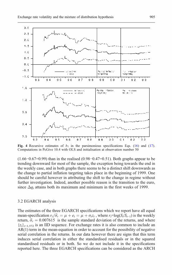
(1.66−0.67=0.99) than in the realised (0.98−0.47=0.51). Both graphs appear to betrending downward for most of the sample, the exception being towards the end inthe weekly case, and in both graphs there seems to be a distinct shift downwards asthe change to partial inflation targeting takes place in the beginning of 1999. Oneshould be careful however in attributing the shift to the change in regime withoutfurther investigation. Indeed, another possible reason is the transition to the euro,since Δqt attains both its maximum and minimum in the first weeks of 1999.

3.2 EGARCH analysis

The estimates of the three EGARCH specifications which we report have all equalmean-specification rt=b�r ¼ �þ et ¼ �þ �tzt , where rt=log(St/St−1) is the weeklyreturn, b�r ¼ 0:007615 is the sample standard deviation of the returns, and where{zt}t=1,572 is an IID sequence. For exchange rates it is also common to include anAR(1) term in the mean-equation in order to account for the possibility of negativeserial correlation in the returns. In our data however there are signs that this terminduces serial correlation in either the standardised residuals or in the squaredstandardised residuals or in both. So we do not include it in the specificationsreported here. The three EGARCH specifications can be considered as the ARCH

Fig. 4 Recursive estimates of b7 in the parsimonious specifications Eqs. (16) and (17).Computations in PcGive 10.4 with OLS and initialisation at observation number 50


counterparts of the weekly log–linear equations, that is, Eqs. (10)–(12), and theirlog-variance specifications are

log �2t ¼ �0 þ �1

et�1

�t�1

��þ �1

et�1

�t�1þ �1 log �

2t�1 þ c11idt þ c12sdt (18)

log �2t ¼ �0 þ �1

et�1

�t�1

��þ �1

et�1

�t�1þ �1 log �

2t�1 þ c1q

�t þ c2�q �

t ð19Þ

þc11 idt þ c12 sdt

log �2t ¼ �0 þ �1

et�1

�t�1

��þ �1

et�1

�t�1þ �1 log �

2t�1 þ c1q

�t þ c2�q �

t

þc3mf �t þ c4o

f �t þ c5x

f �t þ c6u

f �t þ c7f

at þ c8f

at�1 þ c9f

bt

þc10fbt�1 þ c11 idt þ c12 sdt

:

(20)

Specification Eq. (18) is an EGARCH(1,1) with the Russian moratoriumdummy idt and the step dummy sdt as only regressors, Eq. (19) is an EGARCH(1,1)augmented with the quote variables and the dummies, and Eq. (20) is an EGARCH(1,1) with all the economic variables as regressors. Note that * as superscript meansthe variable has been divided by its sample standard deviation. Specifications Eqs.(18)–(20) are analogous to the ARCH-specifications in Lamoureux and Lastrapes(1990), but note that our results are not directly comparable to theirs since ourmeasure of information intensity Δqt does not exhibit strong positive serialcorrelation (in fact, our measure Δqt exhibits weak negative serial correlation).Strong positive serial correlation is an important assumption for their conclusions.

The estimates of Eqs. (18)–(20) are contained in Table 7 and are relativelysimilar significance-wise to the results of the weekly log–linear analysis above, thatis, to the estimates of Eqs. (10)–(12). Note however that the magnitudes of thecoefficient estimates are not directly comparable since the variables are scaleddifferently. The most important similarity is that the coefficient of Δqt

* is positiveand significant in both Eqs. (19) and (20), and that the coefficient estimates arealmost identical in Eqs. (19) and (20). Another important similarity is that themeasure of number of traders qt

* is insignificant in the two EGARCH specificationsin which it is included. There are three minor differences in the inference resultscompared with the weekly log–linear analysis. The first is that the measure of USstock market volatility ut

* is significant at 9% in the EGARCH specificationEq. (20) containing all the variables, whereas it is significant at 1% in the weeklylog–linear counterpart Eq. (12). The second minor difference is that in theEGARCH case the impacts of xt

w* and utw* respectively are not so similar as in the

weekly case. Finally, the step dummy sdt is not significant in the EGARCH spec-ification that only contains the dummies as economic variables, whereas it is in itsweekly counterpart.

There are also some parameters particular to the EGARCH setup that meritattention. The news term et�1=�t�1j j is estimated to be positive as expected and


reasonably similar across the three specifications, but its significance is at theborderline since the two-sided p-values range from 7 to 11%. The impact of theasymmetry term et�1=�t�1 is not significant in any of the equations at conventionalsignificance levels, which suggest no (detectable) asymmetry as is usually foundfor exchange rate data. Persistence is high as suggested by the estimated impact ofthe autoregressive term log σt−1

2 since it is 0.91 in Eq. (18), but it drops to 0.79when the quote variables are included, and then to 0.59 when the rest of theeconomic variables are included, though it remains quite significant in all cases.Finally, the standardised residuals are substantially closer to the normal distributionin Eq. (20) compared with the other two EGARCH specifications.

4 Conclusions

Our study of weekly Norwegian exchange rate volatility sheds new light on themixture of distribution hypothesis in several ways. We find that the impact ofchanges in the number of information events is positive and statistically significantwithin two different frameworks, that the impact is relatively stable across threedifferent exchange rate regimes for both weekly and realised volatility, and that theestimated impacts are relatively similar in both cases. One might have expected thatthe effect of changes in the number of information events would increase with ashift in regime from exchange rate stabilisation to partial inflation targeting, and

Table 7 EGARCH-analysis of NOK/EUR return volatility

(18) (19) (20)


Const. (mean) −0.025 0.37 −0.054 0.05 −0.065 0.01Const. (var.) −0.303 0.11 −0.994 0.13 0.343 0.70∣et−1/σt−1∣ 0.230 0.09 0.247 0.07 0.169 0.11et−1/σt−1 0.005 0.95 0.085 0.21 0.084 0.18log (σt−1

2) 0.906 0.00 0.789 0.00 0.587 0.00qt* 0.038 0.38 0.037 0.49Δqt* 0.373 0.00 0.356 0.00mt

w* 0.148 0.03otw* −0.057 0.29

xtw* 0.312 0.00

utw* 0.098 0.09

fta −0.352 0.71ftb 1.611 0.00idt 3.002 0.00 2.665 0.00 0.441 0.00sdt 0.151 0.19 0.329 0.03 1.552 0.01Log L. −710.16 −687.85 −656.38Q(10) 11.88 0.29 10.95 0.36 11.91 0.29ARCH1−10 0.88 0.55 11.69 0.31 12.46 0.26JB 161.00 0.00 119.73 0.00 20.65 0.00Obs. 572 572 572



then to full inflation targeting, since the Norwegian central bank actively sought tostabilise the exchange rate previous to the full inflation targeting regime. In ourdata however there are no clear breaks, shifts upwards nor trends following thepoints of regime change. Moreover, our results do not support the hypothesis thatan increase in the number of traders reduces volatility. Finally, we have shown thatsimply applying the log of volatility can improve inference and remove undesirableresidual properties. In particular, OLS-estimated autoregressions of the log of vol-atility are capable of producing uncorrelated and (almost) homoscedastic residuals,and in the log of realised volatility case the residuals are also Gaussian.

Our study suggests at least two avenues for future research. First, our resultssuggest there is no impact of the number of traders on exchange rate volatility, butthis might be due to our measure being unsatisfactory. So the first avenue of re-search is to reconsider the hypothesis with a different approach. The second ave-nue of future research is to uncover why applying the log works so well. Pantula(1986), Geweke (1986) and Nelson (1991) proposed that volatility should beanalysed in logs in order to ensure nonnegativity. In our case the motivation stemsfrom unsatisfactory residual properties and fragile inference-results. Before weswitched to the log–linear framework we struggled only to obtain uncorrelatedresiduals within the ARCH, ARMA and linear frameworks, and when we did attainsatisfactory residual properties the results turned out to be very sensitive to smallchanges in the specification. With the log-transformation, however, results are ro-bust across a number of specifications. So the second avenue of further researchconsists of understanding better why the log works. Is it due to particularities in ourdata? For example, is it due to our in financial contexts relatively small sample of573 observations? Is it due to influential observations? Is it due to both? Or is it justdue to the simple fact that applying the log is believed to lead to faster convergencetowards the asymptotic theory which our residual tests rely upon? Further ap-plication of log–linear analysis is necessary in order to answer these questions, andto verify the possible usefulness of the log–linear framework more generally.

Acknowledgements We are indebted to various people for useful comments and suggestions atdifferent stages, including Farooq Akram, Sébastien Laurent, an anonymous referee, participantsat the JAE conference in Venice June 2005, participants at the poster session following the jointCORE-ECARES-KUL seminar in Brussels April 2005, participants at the MICFINMA sum-mer school in Konstanz in June 2004, and participants at the bi-annual doctoral workshop ineconomics at Université catolique de Louvain (Louvain la Neuve) in May 2004. The usual dis-claimer about remaining errors and interpretations being our own applies of course. This work wassupported by the European Community’s Human Potential Programme under contract HPRN-CT-2002-00232, Microstructure of Financial Markets in Europe, and by the Belgian Program onInteruniversity Poles of Attraction initiated by the Belgian State, Prime Minister’s Office, SciencePolicy Programming. The third author would like to thank Finansmarkedsfondet (the NorwegianFinancial Market Fund) and Lånekassen (the Norwegian government’s student funding scheme)for financial support at different stages, and the hospitality of the Department of Economics at theUniversity of Oslo and the Norwegian Central Bank in which part of the research was carried out.


Appendix: Data sources and transformations

The data transformations were undertaken in Ox 3.4 and EViews 5.1.

Sn(t) n(t)=1(t), 2(t),.., N(t), where S1(t) is the first BID NOK/1EUR opening exchange rate ofweek t, S2(t) is the first closing rate, S3(t) is the second opening rate, and so on, with SN(t)denoting the last closing rate of week t. Before 1.1.1999 the BID NOK/1EUR rate isobtained by the formula BID NOK/100DEM×0.0195583, where 0.0195583 is the officialDEM/1EUR conversion rate 1.95583 DEM=1 EUR divided by 100. The first untrans-formed observation is the opening value of BID NOK/100DEM on Wednesday 6.1.1993and the last is the BID NOK/1EUR closing value on Friday 26.12.2003. The source of theBID NOK/100DEM series is Olsen and the source of the BID NOK/1EUR series is Reuters.

St SN(t), the last closing value of week trt log St−log St−1Vt

w {{log[St+I(St=St−1)×0.0009]−log(St−1)} ×100}2. I(St=St−1) is an indicator function equal to1 if St=St−1 and 0 otherwise, and St=St−1 occurs for t=10/6/1994, t=19/8/1994 andt=17/2/2000.

vtw log Vt

w

Vtr Σn [log(Sn/Sn−1)×100]

2, where n=1(t), 2(t),..., N(t) and 1(t)−1≔N(t−1)vtr log Vt

r

Mn(t) n(t)=1(t), 2(t),.., N(t), where M1(t) is the first BID USD/EUR opening exchange rate ofweek t, M2(t) is the first closing rate, M3(t) is the second opening rate, and so on, with MN(t)denoting the last closing rate of week t. Before 1.1.1999 the BID USD/EUR rate is obtainedwith the formula 1.95583/(BID DEM/USD). The first untransformed observation is theopening value of BID DEM/USD on Wednesday 6.1.1993 and the last is the closing valueon Friday 30.12.2003. The source of the BID DEM/USD and BID USD/EUR series isReuters.

Mt MN(t), the last closing value of week tmt log Mt

Mtw {{log[Mt+I(Mt=Mt-1)×kt]−log(Mt-1)}×100}

2. I(Mt=Mt−1) is an indicator function equal to 1if Mt=Mt−1 and 0 otherwise, and kt is a positive number that ensures the log-transformationis not performed on a zero-value. Mt=Mt−1 occurs for t=23/2/1996, t=19/12/1997 andt=20/2/1998, and the value of kt was set on a case to case basis depending on the number ofdecimals in the original, untransformed data series. Specifically the values of kt were set to0.00009, 0.0009 and 0.00009, respectively.

mtw log Mt

w

Mtr Σn [log(Mn/Mn−1)×100]

2, where n =1(t), 2(t),.., N(t) and 1(t)−1≔N(t−1)mt

r log Mtr

Qt Weekly number of NOK/EUR quotes (NOK/100DEM before 1.1.1999). The underlyingdata is a daily series from Olsen Financial Technologies, and the weekly values are obtainedby summing the values of the week.

qt log Qt. Note that this series is “synthetic” in that it has been adjusted for changes in theunderlying quote-collection methodology at Olsen Financial Technologies. More preciselyqt has been generated under the assumption that Δqt was equal to zero in the weekscontaining Friday 17 August 2001 and Friday 5 September 2003, respectively. In the firstweek the underlying feed was changed from Reuters to Tenfore, and on the second a feedfrom Oanda was added.

On(t) n(t)=2(t), 4(t),.., N(t), whereO2(t) is the first closing value of the Brent Blend spot oilprice inUSD per barrel in week t, O4(t) is the second closing value of week t, and so on, with On(t)

denoting the last closing value of week t. The untransformed series is Bank of Norwaydatabase series D2001712, which is based on Telerate page 8891 at 16.00.

Ot ON(t), the last closing value in week tot log Ot

Otw {log[Ot+I(Ot=Ot−1)×0.009]−log(Ot−1) }

2. I(Ot=Ot−1) is an indicator function equal to 1 ifOt=Ot−1 and 0 otherwise, and Ot=Ot−1 occurs three times, for t=1/7/1994, t=13/10/1995 andt=25/7/1997.


otw log Ot

w

Otr Σn [log(On/On−2)]

2, where n=2(t), 4(t),.., N(t) and 2(t)−2≔N(t−1)otr log Ot

r

Xn(t) n(t)=2(t), 4(t),.., N(t), where X2(t) is the first closing value of the main index of theNorwegian Stock Exchange (TOTX) in week t, X4(t) is the second closing value, and so on,with XN(t) denoting the last closing value of week t. The source of the daily untransformedseries is EcoWin series ew:nor15565.

Xt XN(t), the last closing value in week txt log XtXt

w [log (Xt/Xt−1)]2. Xt=Xt−1 does not occur for this series.

xtw log Xt

w

Xtr Σn [log(Xn/Xn−2)]

2, where n=2(t), 4(t),.., N(t) and 2(t)−2≔N(t−1)xtr log Xt

r

Un(t) n(t)=2(t), 4(t),.., N(t), where U2(t) is the first closing value in USD of the composite index ofthe New York Stock Exchange (the NYSE index) in week t, U4(t) is the second closingvalue, and so on, withUN(t) denoting the last closing value of week t. The source of the dailyuntransformed series is EcoWin series ew:usa15540.

Ut UN(t), the last closing value in week tUt

w [log (Ut/Ut-1)]2. Ut=Ut-1 does not occur for this series.

utw log Ut

w

Utr Σn [log(Un/Un−2)]

2, where n=2(t), 4(t),.., N(t) and 2(t)−2≔N(t−1)utr log Ut

r

Ft The Norwegian central bank's main policy interest-rate, the so-called “folio”, at the end ofthe last trading day of week t. The source of the untransformed daily series is Bank ofNorway's web-pages.

fta |Δ Ft|×Ia, where Ia is an indicator function equal to 1 in the period 1 January 1999–Friday

30 March 2001 and 0 elsewhereftb |Δ Ft|×Ib, where Ib is an indicator function equal to 1 after Friday 30 March 2001 and 0

beforeidt Russian moratorium impulse dummy, equal to 1 in the week containing Friday 28 August

1998 and 0 elsewhere.sdt Step dummy, equal to 0 before 1997 and 1 thereafter.

References

Akram QF (2000) When does the oil price affect the Norwegian exchange rate? Working Paper2000/8. The Central Bank of Norway, Oslo

Andersen TG, Bollerslev T, Diebold FS, Labys P(2001) The distribution of realized exchange ratevolatility. J Am Stat Assoc 96:42–55

Bauwens L, Ben Omrane W, Giot P (2005) News announcements, market activity and volatilityin the euro/dollar foreign exchange market. J Int Money Financ, Forthcoming

Bessembinder H, Seguin P (1992) Futures-trading activity and stock price volatility. J Financ47:2015–2034

Bjønnes G, Rime D, Solheim H (2005) Volume and volatility in the FX market: does it matterwho you are? In: De Grauwe P (ed) Exchange rate modelling: where do we stand? MIT Press,Cambridge, MA

Bollerslev T, Wooldridge J (1992) Quasi-maximum likelihood estimation and inference in dy-namic models with time varying covariances. Econ Rev 11:143–172

Bollerslev T, Domowitz I (1993) Trading patterns and prices in the interbank foreign exchangemarket. J Financ 4:1421–1443

Clark P (1973) A subordinated stochastic process model with finite variance for speculativeprices. Econometrica 41:135–155

Demos A, Goodhart CA (1996) The interaction between the frequency of market quotations,spreads and volatility in the foreign exchange market. Appl Econ 28:377–386

Galati (2003) Trading volume, volatility and spreads in foreign exchange markets: evidence fromemerging market countries. BIS Working Paper


Geweke J (1986)Modelling the persistence of conditional variance: a comment. Econ Rev 5:57–61Gilbert CL (1986) Professor Hendry’s econometric methodology. Oxf Bull Econ Stat 48:283–307Giot P (2003) The Asian financial crisis: the start of a regime switch in volatility. CORE

Discussion Paper 2003/78Goodhart C (1991) Every minute counts in financial markets. J Int Money Financ Mark 10:23–52Goodhart C (2000) News and the foreign exchange market. In: Goodhart C (ed) The foreign

exchange market. MacMillan, LondonGrammatikos T, Saunders A (1986) Futures price variability: a test of maturity and volume

effects. J Bus 59:319–330Hendry DF (1995) Dynamic econometrics. Oxford University Press, OxfordHendry DF, Krolzig H-M (2001) Automatic econometric model selection using PcGets.

Timberlake Consultants, LondonJarque C, Bera A (1980) Efficient tests for normality, homoskedasticity, and serial independence

of regression residuals. Econ Lett 6:255–259Jorion P (1996) Risk and turnover in the foreign exchange market. In: Frankel J et al (ed) The

microstructure of foreign exchange markets. University of Chicago Press, ChicagoKarpoff J (1987) The relation between price changes and trading volume: a survey. J Financ

Quant Anal 22:109–126Lamoureux CG, Lastrapes WD (1990) Heteroscedasticity in stock return data: volume versus

GARCH Effects. J Financ, pp 221–229Ljung G, Box G (1979) On a measure of lack of fit in time series models. Biometrika 66:265–270Melvin M, Xixi Y (2000) Public information arrival, exchange rate volatility, and quote

frequency. Econ J 110:644–661Mizon G (1995) Progressive modeling of macroeconomic time series: the LSE methodology. In:

Hoover KD (ed) Macroeconometrics. Developments, tensions and prospects. KluwerNelson DB (1991) Conditional heteroscedasticity in asset returns: a new approach. Econometrica

51:485–505Newey W, West K (1987) A simple positive semi-definite, heteroskedasticity and autocorrelation

consistent covariance matrix. Econometrica 55:703–708Pagan A (1984) Econometric issues in the analysis of regressions with generated regressors. Int

Econ Rev 25:221–247Pantula S (1986) Modelling the persistence of conditional variance: a comment. Econ Rev 5:71–

73Tauchen G, Pitts M (1983) The price variability–volume relationship on speculative markets.

Econometrica 51:485–505White H (1980) A heteroskedasticity-consistent covariance matrix and a direct test for het-

eroskedasticity. Econometrica 48:817–838


exchange rate volatility and the mixture of distribution hypothesis

Documents