exceptionally stable bakelite-type polymers for efficient ... · exceptionally stable bakelite-type...
TRANSCRIPT

Supporting Information for
Exceptionally Stable Bakelite-type Polymers for Efficient
Pre-Combustion CO2 Capture and H2 Purification
Shyamapada Nandi,a Jens Rother,
c Debanjan Chakraborty,
a Rahul Maity,
a Ulrike Werner-
Zwanziger,d Ramanathan Vaidhyanathan
ab*
a Department of Chemistry, Indian Institute of Science Education and Research, Pune, Dr. Homi Bhabha Rd.,
Pashan, Pune, MH, India, 411008. b Centre for Research in Energy and Sustainable Materials, Centre for Energy Science, Indian Institute of Science
Education and Research, Pune, Dr. Homi Bhabha Rd., Pashan, Pune, MH, India, 411008. c Rubolab GmbH, Neckarstr. 27, 40219 Düsseldorf, Germany.
d Department of Chemistry, IRM, NMR-3, Dalhousie University, 6274 Coburg Road, PO BOX 15000, Halifax, NS
B3H4R2, Canada.
E-mail: [email protected]
Table of contents:
1. Materials and methods
2. Analytical characterizations: Powder diffraction, TGA studies, IR-spectra and Solid State
NMR
3. Adsorption studies
4. Heat of adsorption for CO2 from Virial and NLDFT models
5. Selectivity Calculation; Ideal Adsorption Solution Theory(IAST):
6. Contact angle measurement
7. TGA cycling experiments (CO2 adsorption-desorption)
8. Steam conditioning experiments:
9. Rate of adsorption studies- self-diffusion coefficients calculations and analysis
10. Stability study
11. Breakthrough (Mixed Gas) Analysis
12. Computational details
Electronic Supplementary Material (ESI) for Journal of Materials Chemistry A.This journal is © The Royal Society of Chemistry 2017
1. Materials and Methods:
All the organic chemicals were purchased from sigma aldrich. 4,4',4''-(1,3,5-triazine-
2,4,6-triyl)tris(benzene-1,3-diol) and 4,4',4''-(1,3,5-triazine-2,4,6-triyl)tris(benzene-1,3,5-triol)
was synthesized according to previously reported procedure(S1and 50).
S1: Nandi et al., Adv. Mater. Interfaces 2015, 2, 1500301.
Synthesis of HPF-3:
A solvothermal reaction between 4,4',4''-(1,3,5-triazine-2,4,6-triyl)tris(benzene-1,3,5-
triol) (0.228g; 0.5mmol) and 4-(4-Formylphenoxy)benzaldehyde (0.170g; 0.75mmol) in a
solution containing 5ml 1,4-dioxane + 5ml tetrahydrofuran (THF) and 0.25 ml of acetic acid was
carried out at 200oC for 72hrs. Yellowish red colored powder was isolated by filtration and was
washed with Dimethylformamide (DMF) (20ml), THF(50ml) and finally with plenty of
methanol and acetone. The dried sample gave a yield of ~79%. CHN analysis (calculated values
within brackets): C: 67.96 (68.29); H: 3.49 (3.27); N: 5.95 (5.69)%. Note: Before the CHN
analyses, the samples were washed with hot DMF, exchanged with methanol and then dried
under vacuum. Some discrepancies between the calculated and observed values can be attributed
to the presence of few unreacted terminal aldehydes, this is consistent with our observations
from NMR and IR.
Synthesis of HPF-4:
A solvothermal reaction between 4,4',4''-(1,3,5-triazine-2,4,6-triyl)tris(benzene-1,3-diol)
(0.203g; 0.5mmol) and 4-(4-Formylphenoxy)benzaldehyde (0.170g; 0.75mmol) in a solution
containing 5ml 1,4-dioxane + 5ml tetrahydrofuran (THF) and 0.25 ml of acetic acid was carried
out at 200oC for 72hrs. Bright yellowish colored powder was isolated by filtration and was
washed with Dimethylformamide (DMF) (20ml), THF (50ml) and finally with plenty of
methanol and acetone. The dried sample gave a yield of ~82%. CHN analysis (calculated values
within brackets): C: 76.72 (76.59); H: 3.67 (3.67); N: 6.45 (6.38)%.
Synthesis of HPF-5:
A solvothermal reaction between 2,2′,4,4′-Tetrahydroxybenzophenone (0.246g;
1.0mmol) and 4-(4-Formylphenoxy)benzaldehyde (0.226g; 1.0mmol) in a solution containing
5ml 1,4-dioxane + 5ml tetrahydrofuran (THF) and 0.25 ml of acetic acid was carried out at
200oC for 72hrs. Bright red colored powder was isolated by filtration and was washed with
Dimethylformamide (DMF) (20ml), THF (50ml) and finally with plenty of methanol and
acetone. The dried sample gave a yield of ~86%. CHN analysis (calculated values within
brackets): C: 73.96 (74.31); H: 3.65 (3.70)%.
Note: All three polymers were subjected to a soxhlation as a cleaning procedure.
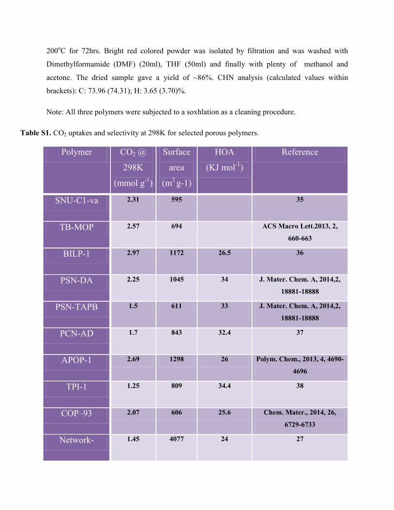
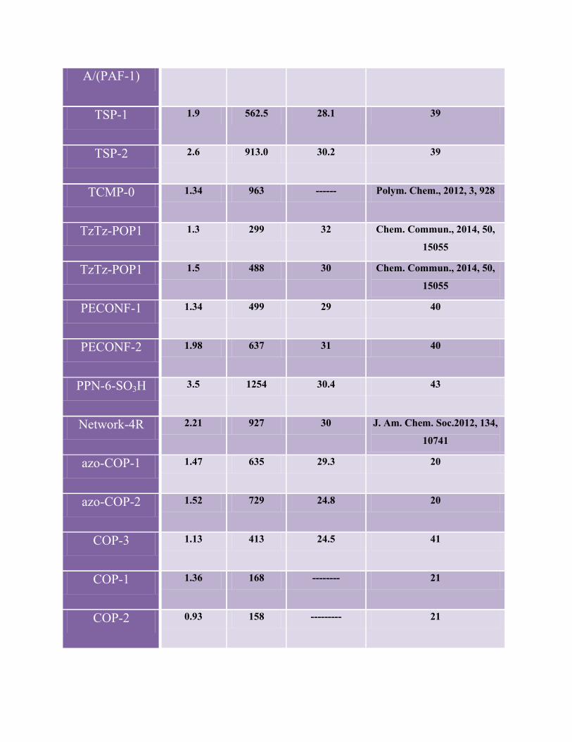
Table S1. CO2 uptakes and selectivity at 298K for selected porous polymers.
Polymer CO2 @
298K
(mmol g-1
)
Surface
area
(m2 g-1)
HOA
(KJ mol-1
)
Reference
SNU-C1-va 2.31 595 35
TB-MOP 2.57 694 ACS Macro Lett.2013, 2,
660-663
BILP-1 2.97 1172 26.5 36
PSN-DA 2.25 1045 34 J. Mater. Chem. A, 2014,2,
18881-18888
PSN-TAPB 1.5 611 33 J. Mater. Chem. A, 2014,2,
18881-18888
PCN-AD 1.7 843 32.4 37
APOP-1 2.69 1298 26 Polym. Chem., 2013, 4, 4690-
4696
TPI-1 1.25 809 34.4 38
COP–93 2.07 606 25.6 Chem. Mater., 2014, 26,
6729-6733
Network- 1.45 4077 24 27
A/(PAF-1)
TSP-1 1.9 562.5 28.1 39
TSP-2 2.6 913.0 30.2 39
TCMP-0 1.34 963 ------ Polym. Chem., 2012, 3, 928
TzTz-POP1 1.3 299 32 Chem. Commun., 2014, 50,
15055
TzTz-POP1 1.5 488 30 Chem. Commun., 2014, 50,
15055
PECONF-1 1.34 499 29 40
PECONF-2 1.98 637 31 40
PPN-6-SO3H 3.5 1254 30.4 43
Network-4R 2.21 927 30 J. Am. Chem. Soc.2012, 134,
10741
azo-COP-1 1.47 635 29.3 20
azo-COP-2 1.52 729 24.8 20
COP-3 1.13 413 24.5 41
COP-1 1.36 168 -------- 21
COP-2 0.93 158 --------- 21
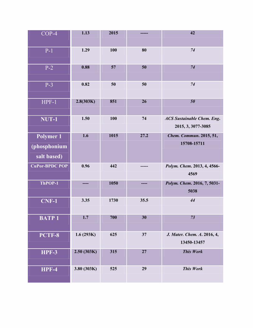
COP-4 1.13 2015 ----- 42
P-1 1.29 100 80 74
P-2 0.88 57 50 74
P-3 0.82 50 50 74
HPF-1 2.8(303K) 851 26 50
NUT-1 1.50 100 74 ACS Sustainable Chem. Eng.
2015, 3, 3077-3085
Polymer 1
(phosphonium
salt based)
1.6 1015 27.2 Chem. Commun. 2015, 51,
15708-15711
CuPor-BPDC POP 0.96 442 ----- Polym. Chem. 2013, 4, 4566-
4569
ThPOP-1 ---- 1050 ---- Polym. Chem. 2016, 7, 5031-
5038
CNF-1 3.35 1730 35.5 44
BATP 1 1.7 700 30 73
PCTF-8 1.6 (293K) 625 37 J. Mater. Chem. A. 2016, 4,
13450-13457
HPF-3 2.50 (303K) 315 27 This Work
HPF-4 3.80 (303K) 525 29 This Work

HPF-5 3.01 (303K) 516 32 This Work
------- = Data not available.
2. Analytical Characterizations:
Powder X-ray diffraction:
Powder XRDs were carried out using a Rigaku Miniflex-600 instrument and processed
using PDXL software.
Thermogravimetric Analysis (TGA):
Thermogravimetry was carried out on NETSZCH TGA-DSC system. The conventional
TGA experiments were done under N2 gas flow (20 ml min-1
) (purge + protective) and samples
were heated from RT to 550oC at 2 K min
-1.
Infrared Spectroscopy:
IR spectra were obtained using a Nicolet ID5 attenuated total reflectance IR spectrometer
operating at ambient temperature. The anhydrous KBr pellets were used.
Solid State NMR Spectroscopy:
All NMR experiments were carried out on a Bruker Advance NMR spectrometer with a
9.4T magnet (400.24 MHz proton Larmor frequency, 100.64MHz 13
C Larmor frequency) using
our probe head for rotors of 4 mm diameter. The parameters for the 13
C CP/MAS experiments
with TPPM proton decoupling were optimized on glycine, whose carbonyl resonance also served
as external, secondary chemical shift standard at 176.06 ppm. For the final 13
C CP/MAS NMR
spectra up to 600 scans were acquired at 3.1 s recycle delay. The sample was spun at 7.0, 8.0,
and 13.3 kHz rotation frequencies to separate isotropic shift peaks and spinning sidebands.
Spinning sidebands were separated from the isotropic shift peak by a multiple of the rotation
frequency. The cross-polarization contact time was chosen to be 2.6 ms, to obtain a good balance
between detecting carbons with directly bonded protons and other carbons, for which protons are
further removed.
Field Emission-SEM:
Field Emission Scanning Electron Microscope with integral charge compensator and
embedded EsB and AsB detectors. Oxford X-max instruments 80mm2. (Carl Zeiss NTS, Gmbh),
Imagin conditions: 3kV, WD= 2mm, 200kX, SE lens detector. For SEM images sample was

grind nicely and soaked in THF for 12 hrs. Then filtered and dried in hot oven at 90oC. The fine
powder was spread over carbon paper and SEM images were taken at different range.
Figure S1. Powder X-ray diffraction patterns of HPF-3 indicating its amorphous character. The big hump
at around 2 = 20o is from the polymer and is not from the glass substrate. Plenty of sample was used
during the experiment.
Figure S2. Powder X-ray diffraction patterns of HPF-4 showing its amorphous character.

Figure S3. Powder X-ray diffraction patterns of HPF-5 showing the amorphous nature of the sample.
Figure S4. FE-SEM images of (A) HPF-3, (B) HPF-4, (C) HPF-5 microspheres indicating high
homogeneity as well as purity of the sample. The sizes of the microspheres are distributed between 0.3 to
5microns.
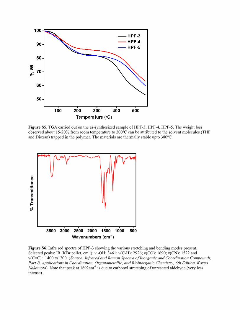
Figure S5. TGA carried out on the as-synthesized sample of HPF-3, HPF-4, HPF-5. The weight loss
observed about 15-20% from room temperature to 200oC can be attributed to the solvent molecules (THF
and Dioxan) trapped in the polymer. The materials are thermally stable upto 380ºC.
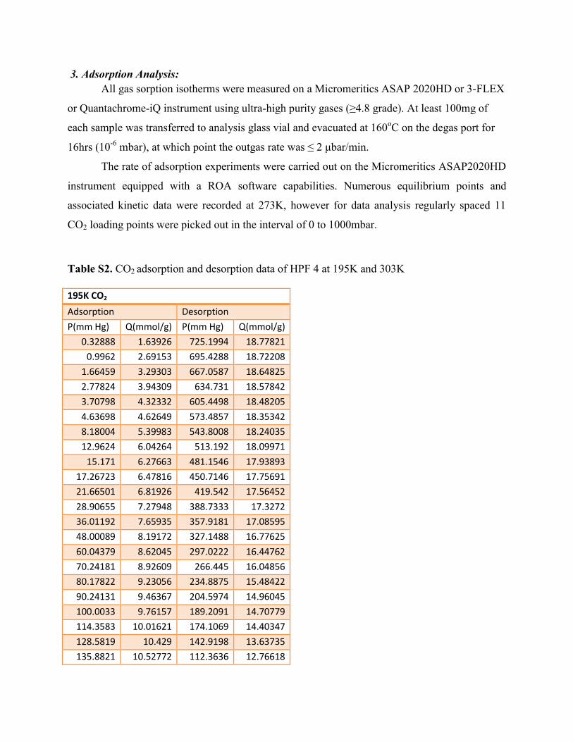
Figure S6. Infra red spectra of HPF-3 showing the various stretching and bending modes present.
Selected peaks: IR (KBr pellet, cm-1
): ν -OH: 3461; ν(C-H): 2926; ν(CO): 1690; ν(CN): 1522 and
v(C=C): 1400 to1200. (Source: Infrared and Raman Spectra of Inorganic and Coordination Compounds,
Part B, Applications in Coordination, Organometallic, and Bioinorganic Chemistry, 6th Edition, Kazuo
Nakamoto). Note that peak at 1692cm-1
is due to carbonyl stretching of unreacted aldehyde (very less
intense).

Figure S7. Infra red spectra of HPF-4 showing the various stretching and bending modes present.
Selected peaks: IR (KBr pellet, cm-1
): ν(O-H)solvent and -OH: 3472; ν(C-H): 2922; ν(CO): 1684; ν(CN):
1522 and v(C=C): 1400 to1200. (Source: Infrared and Raman Spectra of Inorganic and Coordination
Compounds, Part B, Applications in Coordination, Organometallic, and Bioinorganic Chemistry, 6th
Edition, Kazuo Nakamoto). Note that peak at 1692cm-1
is due to carbonyl stretching of unreacted
aldehyde (very less intense).
Figure S8. Infra red spectra of HPF-5 showing the various stretching and bending modes present.
Selected peaks: IR (KBr pellet, cm-1
): ν(O-H)solvent and -OH: 3486; ν(C-H): 2921; ν(CO): 1652; ν(CN):
1520 and v(C=C): 1400 to1200. (Source: Infrared and Raman Spectra of Inorganic and Coordination
Compounds, Part B, Applications in Coordination, Organometallic, and Bioinorganic Chemistry, 6th
Edition, Kazuo Nakamoto). Note that peak at 1692cm-1
is due to carbonyl stretching of unreacted
aldehyde (very less intense).
3. Adsorption Analysis:
All gas sorption isotherms were measured on a Micromeritics ASAP 2020HD or 3-FLEX
or Quantachrome-iQ instrument using ultra-high purity gases (≥4.8 grade). At least 100mg of
each sample was transferred to analysis glass vial and evacuated at 160oC on the degas port for
16hrs (10-6
mbar), at which point the outgas rate was ≤ 2 μbar/min.
The rate of adsorption experiments were carried out on the Micromeritics ASAP2020HD
instrument equipped with a ROA software capabilities. Numerous equilibrium points and
associated kinetic data were recorded at 273K, however for data analysis regularly spaced 11
CO2 loading points were picked out in the interval of 0 to 1000mbar.
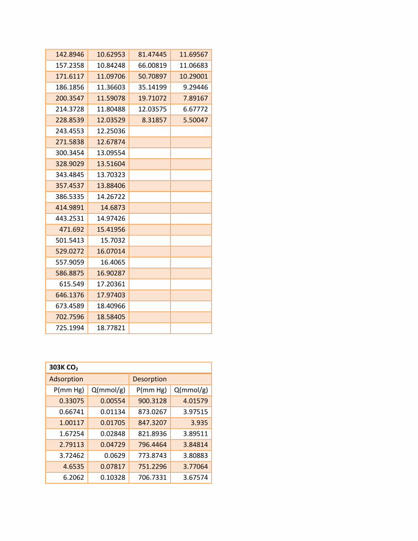
Table S2. CO2 adsorption and desorption data of HPF 4 at 195K and 303K
195K CO2
Adsorption Desorption
P(mm Hg) Q(mmol/g) P(mm Hg) Q(mmol/g)
0.32888 1.63926 725.1994 18.77821
0.9962 2.69153 695.4288 18.72208
1.66459 3.29303 667.0587 18.64825
2.77824 3.94309 634.731 18.57842
3.70798 4.32332 605.4498 18.48205
4.63698 4.62649 573.4857 18.35342
8.18004 5.39983 543.8008 18.24035
12.9624 6.04264 513.192 18.09971
15.171 6.27663 481.1546 17.93893
17.26723 6.47816 450.7146 17.75691
21.66501 6.81926 419.542 17.56452
28.90655 7.27948 388.7333 17.3272
36.01192 7.65935 357.9181 17.08595
48.00089 8.19172 327.1488 16.77625
60.04379 8.62045 297.0222 16.44762
70.24181 8.92609 266.445 16.04856
80.17822 9.23056 234.8875 15.48422
90.24131 9.46367 204.5974 14.96045
100.0033 9.76157 189.2091 14.70779
114.3583 10.01621 174.1069 14.40347
128.5819 10.429 142.9198 13.63735
135.8821 10.52772 112.3636 12.76618
142.8946 10.62953 81.47445 11.69567
157.2358 10.84248 66.00819 11.06683
171.6117 11.09706 50.70897 10.29001
186.1856 11.36603 35.14199 9.29446
200.3547 11.59078 19.71072 7.89167
214.3728 11.80488 12.03575 6.67772
228.8539 12.03529 8.31857 5.50047
243.4553 12.25036
271.5838 12.67874
300.3454 13.09554
328.9029 13.51604
343.4845 13.70323
357.4537 13.88406
386.5335 14.26722
414.9891 14.6873
443.2531 14.97426
471.692 15.41956
501.5413 15.7032
529.0272 16.07014
557.9059 16.4065
586.8875 16.90287
615.549 17.20361
646.1376 17.97403
673.4589 18.40966
702.7596 18.58405
725.1994 18.77821
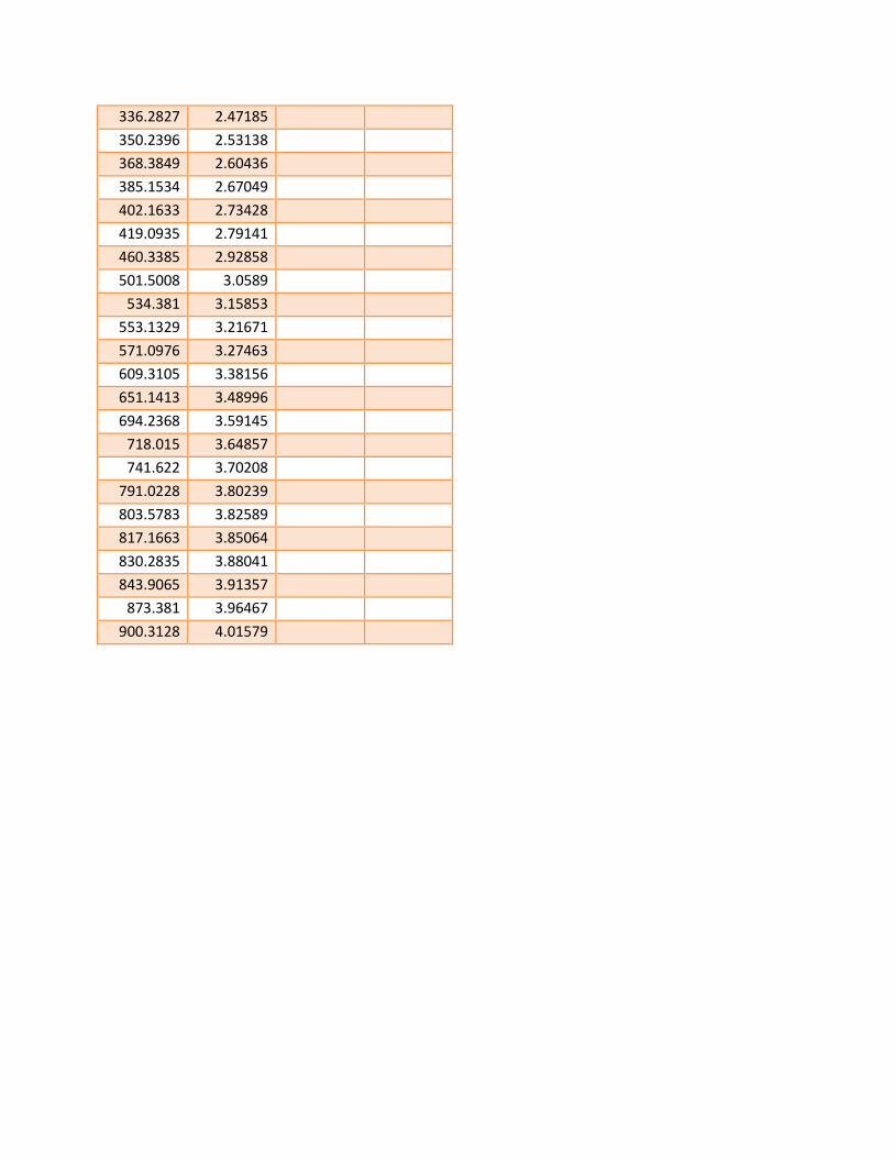
303K CO2
Adsorption Desorption
P(mm Hg) Q(mmol/g) P(mm Hg) Q(mmol/g)
0.33075 0.00554 900.3128 4.01579
0.66741 0.01134 873.0267 3.97515
1.00117 0.01705 847.3207 3.935
1.67254 0.02848 821.8936 3.89511
2.79113 0.04729 796.4464 3.84814
3.72462 0.0629 773.8743 3.80883
4.6535 0.07817 751.2296 3.77064
6.2062 0.10328 706.7331 3.67574

7.76351 0.13002 626.2682 3.49958
10.33902 0.15753 590.2872 3.40473
13.09543 0.19436 555.0627 3.30978
15.34408 0.22445 492.1578 3.13274
17.49938 0.25366 436.0129 2.953
19.64794 0.28155 386.6693 2.77102
21.76053 0.31033 342.3257 2.59696
25.51796 0.35593 303.583 2.43304
29.0541 0.39634 269.2248 2.26963
32.60812 0.43514 238.4738 2.113
36.23187 0.47699 211.4889 1.9631
42.23356 0.54833 187.4097 1.81748
48.2729 0.61576 166.2157 1.68153
51.14283 0.6466 147.2541 1.54985
54.1335 0.67924 130.6826 1.42726
60.20168 0.74281 115.8427 1.311
65.40663 0.7948 102.6561 1.20645
70.31162 0.83974 91.00278 1.10643
75.31184 0.8857 80.66891 1.01123
80.3195 0.93222 71.52169 0.92491
90.25084 1.01914 63.36257 0.84436
100.464 1.10495 56.17084 0.76606
110.3869 1.18389 49.77603 0.6941
120.1214 1.25753 18.5325 0.324
131.9006 1.34513 7.0748 0.16173
143.6 1.42847 2.65575 0.07423
157.5587 1.5254 1.00295 0.03021
171.495 1.62267
188.497 1.7292
196.5463 1.77831
204.7115 1.82664
215.0884 1.88397
225.1633 1.93762
234.8855 1.98934
244.8702 2.04157
256.926 2.10459
280.7437 2.21862
292.8107 2.27112
307.571 2.33997
321.7351 2.40347
336.2827 2.47185
350.2396 2.53138
368.3849 2.60436
385.1534 2.67049
402.1633 2.73428
419.0935 2.79141
460.3385 2.92858
501.5008 3.0589
534.381 3.15853
553.1329 3.21671
571.0976 3.27463
609.3105 3.38156
651.1413 3.48996
694.2368 3.59145
718.015 3.64857
741.622 3.70208
791.0228 3.80239
803.5783 3.82589
817.1663 3.85064
830.2835 3.88041
843.9065 3.91357
873.381 3.96467
900.3128 4.01579
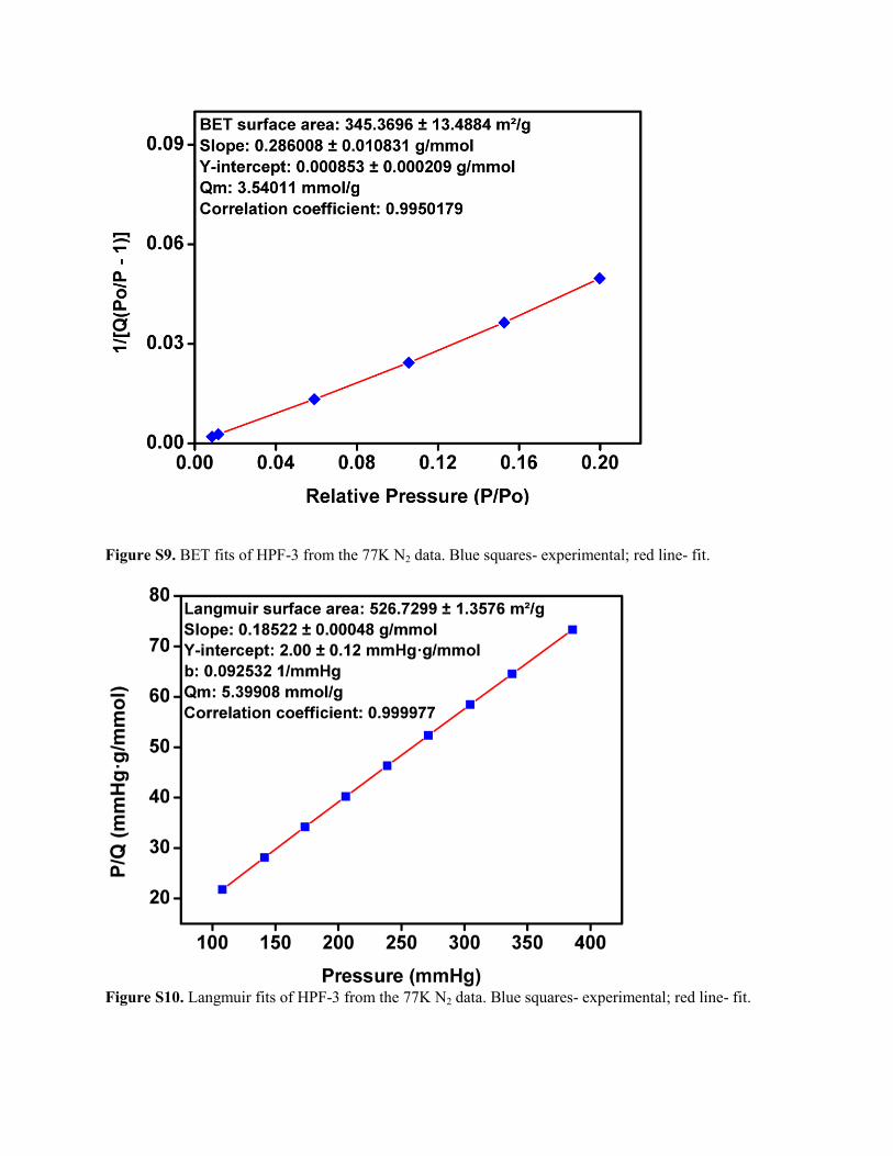
Figure S9. BET fits of HPF-3 from the 77K N2 data. Blue squares- experimental; red line- fit.
Figure S10. Langmuir fits of HPF-3 from the 77K N2 data. Blue squares- experimental; red line- fit.
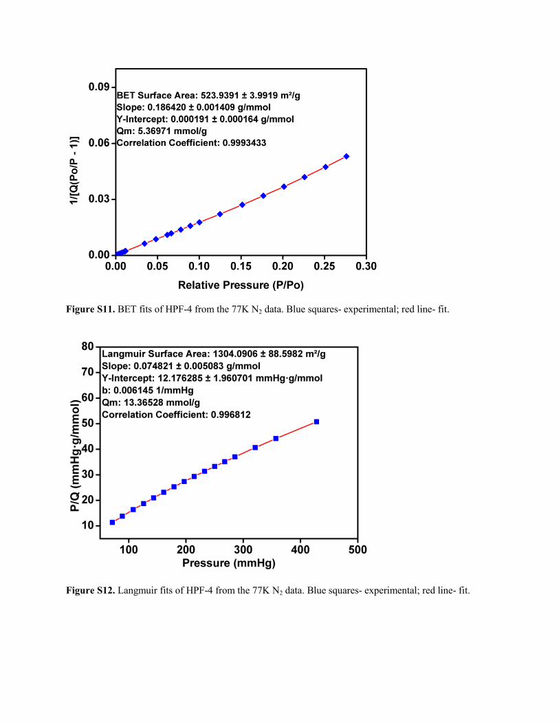
Figure S11. BET fits of HPF-4 from the 77K N2 data. Blue squares- experimental; red line- fit.
Figure S12. Langmuir fits of HPF-4 from the 77K N2 data. Blue squares- experimental; red line- fit.
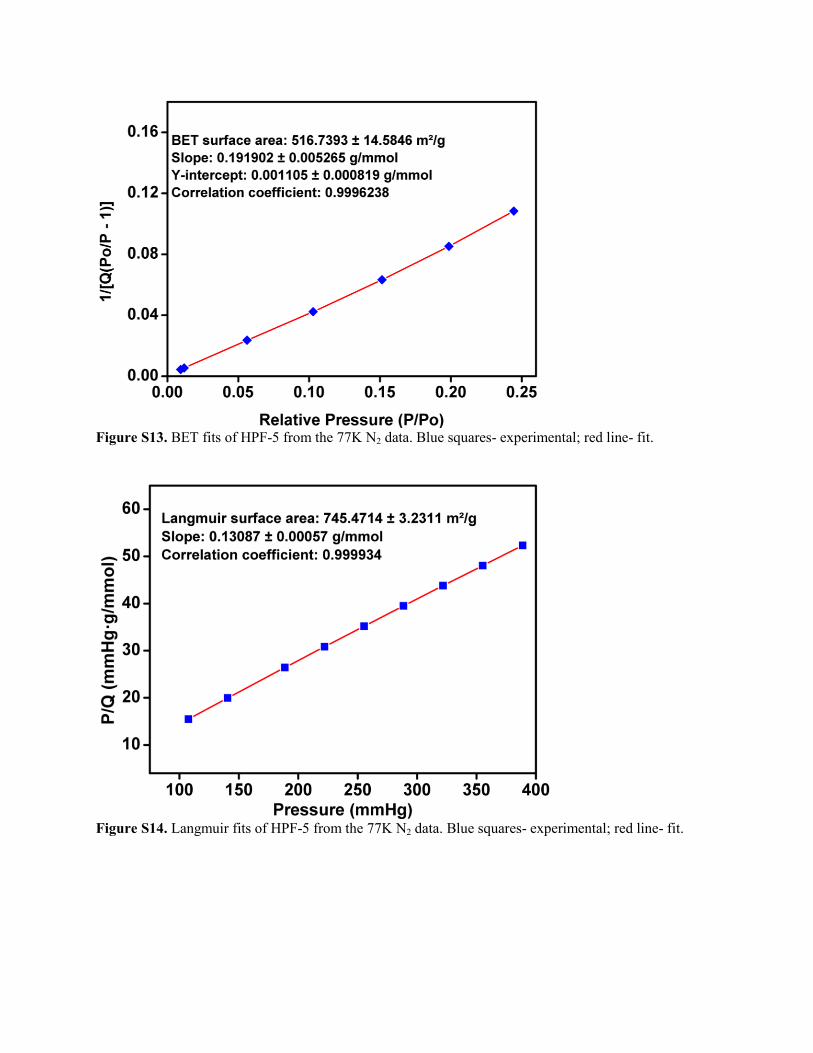
Figure S13. BET fits of HPF-5 from the 77K N2 data. Blue squares- experimental; red line- fit.
Figure S14. Langmuir fits of HPF-5 from the 77K N2 data. Blue squares- experimental; red line- fit.

Figure S15. QSDFT fits for the 273K CO2 and 77K N2 isotherms obtained using a Carbon
model.
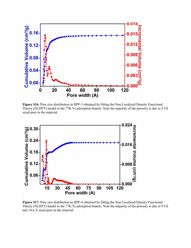
Figure S16. Pore size distribution in HPF-3 obtained by fitting the Non Localized Density Functional
Theory (NLDFT) model to the 77K N2 adsorption branch. Note the majority of the porosity is due to 5.5Å
sized pore in the material.
.
Figure S17. Pore size distribution in HPF-4 obtained by fitting the Non Localized Density Functional
Theory (NLDFT) model to the 77K N2 adsorption branch. Note the majority of the porosity is due to 9.5Å
and 14.6 Å sized pore in the material.
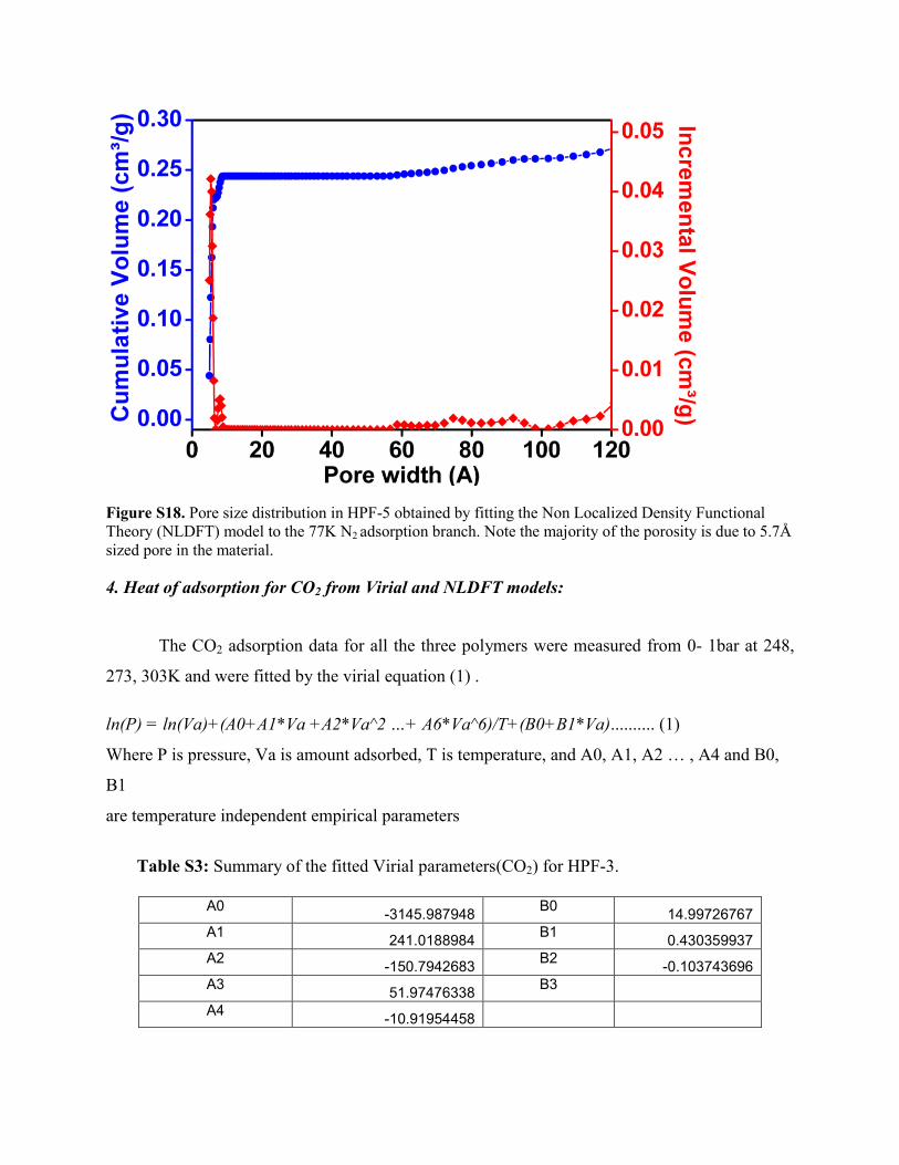
Figure S18. Pore size distribution in HPF-5 obtained by fitting the Non Localized Density Functional
Theory (NLDFT) model to the 77K N2 adsorption branch. Note the majority of the porosity is due to 5.7Å
sized pore in the material.
4. Heat of adsorption for CO2 from Virial and NLDFT models:
The CO2 adsorption data for all the three polymers were measured from 0- 1bar at 248,
273, 303K and were fitted by the virial equation (1) .
ln(P) = ln(Va)+(A0+A1*Va +A2*Va^2 …+ A6*Va^6)/T+(B0+B1*Va).......... (1)
Where P is pressure, Va is amount adsorbed, T is temperature, and A0, A1, A2 … , A4 and B0,
B1
are temperature independent empirical parameters
Table S3: Summary of the fitted Virial parameters(CO2) for HPF-3.
A0
-3145.987948 B0
14.99726767
A1 241.0188984
B1 0.430359937
A2 -150.7942683
B2 -0.103743696
A3 51.97476338
B3
A4 -10.91954458
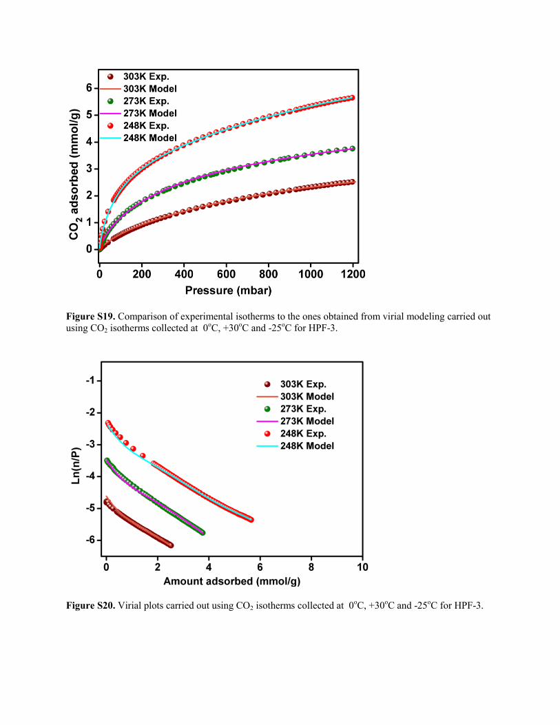
Figure S19. Comparison of experimental isotherms to the ones obtained from virial modeling carried out
using CO2 isotherms collected at 0oC, +30
oC and -25
oC for HPF-3.
Figure S20. Virial plots carried out using CO2 isotherms collected at 0
oC, +30
oC and -25
oC for HPF-3.
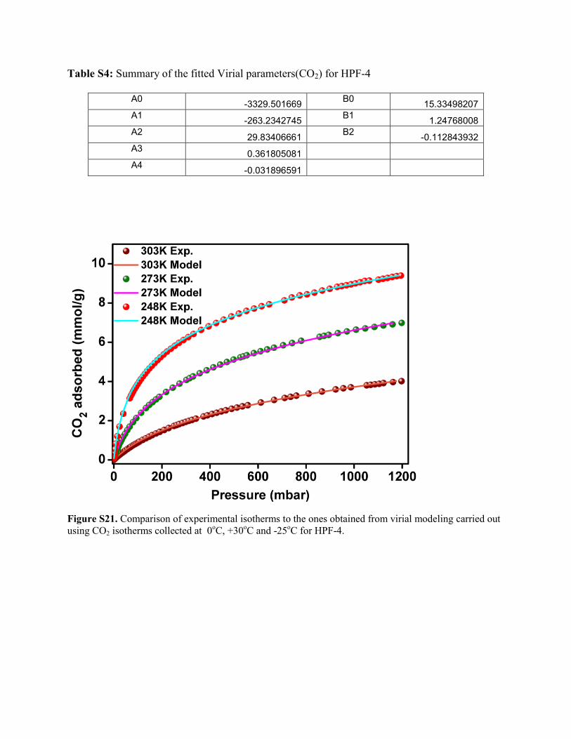
Table S4: Summary of the fitted Virial parameters(CO2) for HPF-4
A0
-3329.501669 B0
15.33498207
A1 -263.2342745
B1 1.24768008
A2 29.83406661
B2 -0.112843932
A3 0.361805081
A4 -0.031896591
Figure S21. Comparison of experimental isotherms to the ones obtained from virial modeling carried out
using CO2 isotherms collected at 0oC, +30
oC and -25
oC for HPF-4.
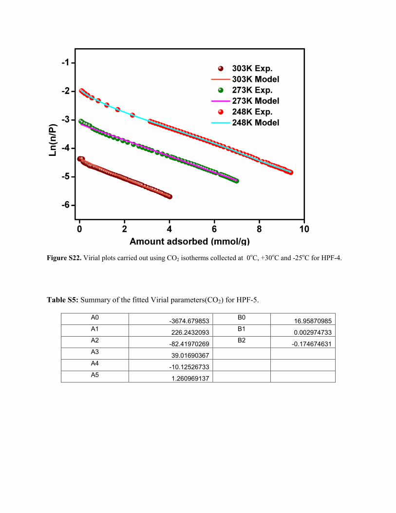
Figure S22. Virial plots carried out using CO2 isotherms collected at 0oC, +30
oC and -25
oC for HPF-4.
Table S5: Summary of the fitted Virial parameters(CO2) for HPF-5.
A0
-3674.679853 B0
16.95870985
A1 226.2432093
B1 0.002974733
A2 -82.41970269
B2 -0.174674631
A3 39.01690367
A4 -10.12526733
A5 1.260969137
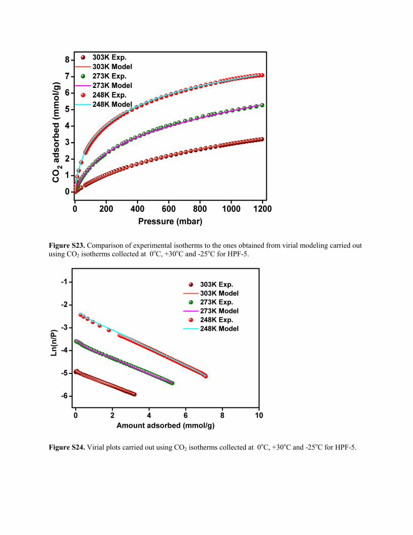
Figure S23. Comparison of experimental isotherms to the ones obtained from virial modeling carried out
using CO2 isotherms collected at 0oC, +30
oC and -25
oC for HPF-5.
Figure S24. Virial plots carried out using CO2 isotherms collected at 0oC, +30
oC and -25
oC for HPF-5.

Table S6: Summary of the fitted Virial parameters(toluene) for HPF-3
A0
-10431.88245 B0
28.77813374
A1 3521.322573
B1 -2.637644719
A2 -773.2662505
B2 -1.990529606
A3 211.0338766
B3 0.465026047
A4 -35.95388903
A5 2.298304647
Figure S25. Virial plots carried out using water isotherms collected at +25
oC and +35
oC for HPF-3.

Table S7: Summary of the fitted Virial parameters(toluene) for HPF-4
A0
-10402.19379 B0
27.89899548
A1 379.6048987
B1 2.738091842
A2 261.3025532
B2 -1.703546217
A3 -11.91991164
B3 0.125615738
A4 -1.307962347
A5 ----
Figure S26. Virial plots carried out using water isotherms collected at +25
oC and +35
oC for HPF-4.

Table S8: Summary of the fitted Virial parameters(toluene) for HPF-5
A0
-9169.517361 B0
23.3334306
A1 684.5924201
B1 2.505867035
A2 97.84135297
B2 -1.5126849
A3 12.76732157
B3 0.112948228
A4 -3.202179048
A5 ----
Figure S27. Virial plots carried out using water isotherms collected at +25
oC and +35
oC for HPF-5.

Table S9: Summary of the fitted Virial parameters(Water) for HPF-3
A0
-5557.334612 B0
17.90471422
A1 106.0990556
B1 2.851214141
A2 -61.98277468
B2 -2.446088567
A3 18.80785699
B3 0.985661022
A4 -29.51765718
A5 6.642661404
Figure S28. Virial plots carried out using water isotherms collected at +25oC and +35
oC for HPF-3.
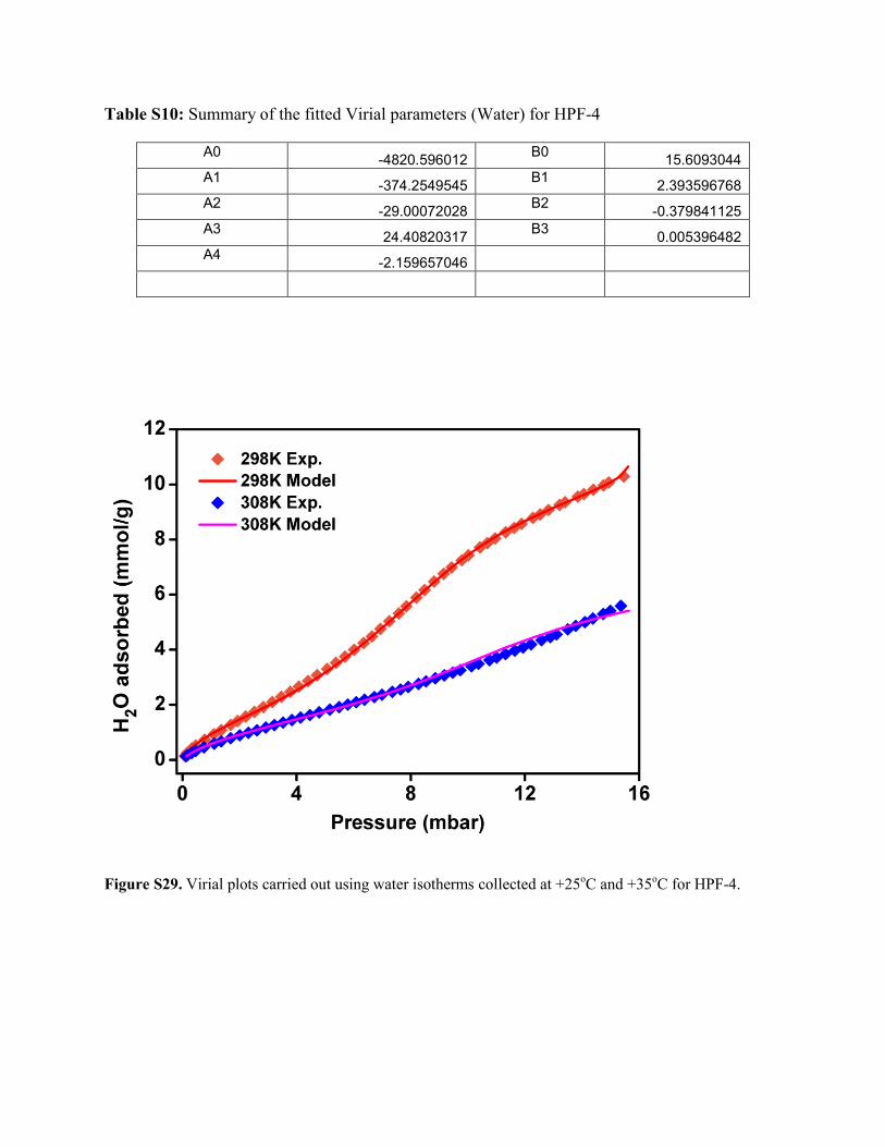
Table S10: Summary of the fitted Virial parameters (Water) for HPF-4
A0 -4820.596012
B0 15.6093044
A1 -374.2549545
B1 2.393596768
A2 -29.00072028
B2 -0.379841125
A3 24.40820317
B3 0.005396482
A4 -2.159657046
Figure S29. Virial plots carried out using water isotherms collected at +25oC and +35
oC for HPF-4.

Table S11: Summary of the fitted Virial parameters (Water) for HPF-5
A0
-7150.906388 B0
23.11851189
A1 603.4940537
B1 -0.471299064
A2 -7.320758651
B2 -0.677172212
A3 7.528813204
B3 0.135519672
A4 -6.08168734
A5 0.405792751
Figure S30. Virial plots carried out using water isotherms collected at +25oC and +35
oC for HPF-5.
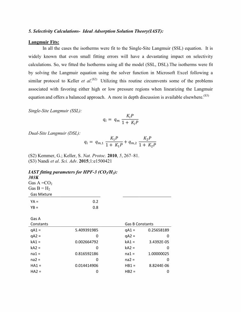
5. Selectivity Calculations- Ideal Adsorption Solution Theory(IAST):
Langmuir Fits:
In all the cases the isotherms were fit to the Single-Site Langmuir (SSL) equation. It is
widely known that even small fitting errors will have a devastating impact on selectivity
calculations. So, we fitted the Isotherms using all the model (SSL, DSL).The isotherms were fit
by solving the Langmuir equation using the solver function in Microsoft Excel following a
similar protocol to Keller et al.(S2)
Utilizing this routine circumvents some of the problems
associated with favoring either high or low pressure regions when linearizing the Langmuir
equation and offers a balanced approach. A more in depth discussion is available elsewhere.
(S3)
Single-Site Langmuir (SSL):
Dual-Site Langmuir (DSL):
(S2) Kemmer, G.; Keller, S. Nat. Protoc. 2010, 5, 267–81.
(S3) Nandi et al. Sci. Adv. 2015;1:e1500421
IAST fitting parameters for HPF-3 (CO2/H2):
303K
Gas A =CO2
Gas B = H2
Gas Mixture YA = 0.2 YB = 0.8
Gas A Constants Gas B Constants
qA1 = 5.409391985
qA1 = 0.25658189 qA2 = 0
qA2 = 0
kA1 = 0.002664792
kA1 = 3.4392E-05 kA2 = 0
kA2 = 0
na1 = 0.816592186
na1 = 1.00000025 na2 = 0
na2 = 0
HA1 = 0.014414906
HB1 = 8.8244E-06 HA2 = 0
HB2 = 0
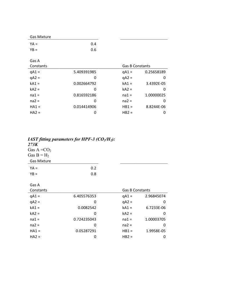
Gas Mixture YA = 0.4 YB = 0.6
Gas A Constants Gas B Constants
qA1 = 5.409391985
qA1 = 0.25658189 qA2 = 0
qA2 = 0
kA1 = 0.002664792
kA1 = 3.4392E-05 kA2 = 0
kA2 = 0
na1 = 0.816592186
na1 = 1.00000025
na2 = 0
na2 = 0 HA1 = 0.014414906
HB1 = 8.8244E-06
HA2 = 0
HB2 = 0
IAST fitting parameters for HPF-3 (CO2/H2):
273K
Gas A =CO2
Gas B = H2
Gas Mixture YA = 0.2 YB = 0.8
Gas A Constants Gas B Constants
qA1 = 6.405576353
qA1 = 2.96845074
qA2 = 0
qA2 = 0 kA1 = 0.0082542
kA1 = 6.7233E-06
kA2 = 0
kA2 = 0 na1 = 0.724235043
na1 = 1.00003705
na2 = 0
na2 = 0 HA1 = 0.05287291
HB1 = 1.9958E-05
HA2 = 0
HB2 = 0
Gas Mixture YA = 0.4 YB = 0.6
Gas A Constants Gas B Constants
qA1 = 6.405576353
qA1 = 2.96845074 qA2 = 0
qA2 = 0
kA1 = 0.0082542
kA1 = 6.7233E-06 kA2 = 0
kA2 = 0
na1 = 0.724235043
na1 = 1.00003705 na2 = 0
na2 = 0
HA1 = 0.05287291
HB1 = 1.9958E-05 HA2 = 0
HB2 = 0
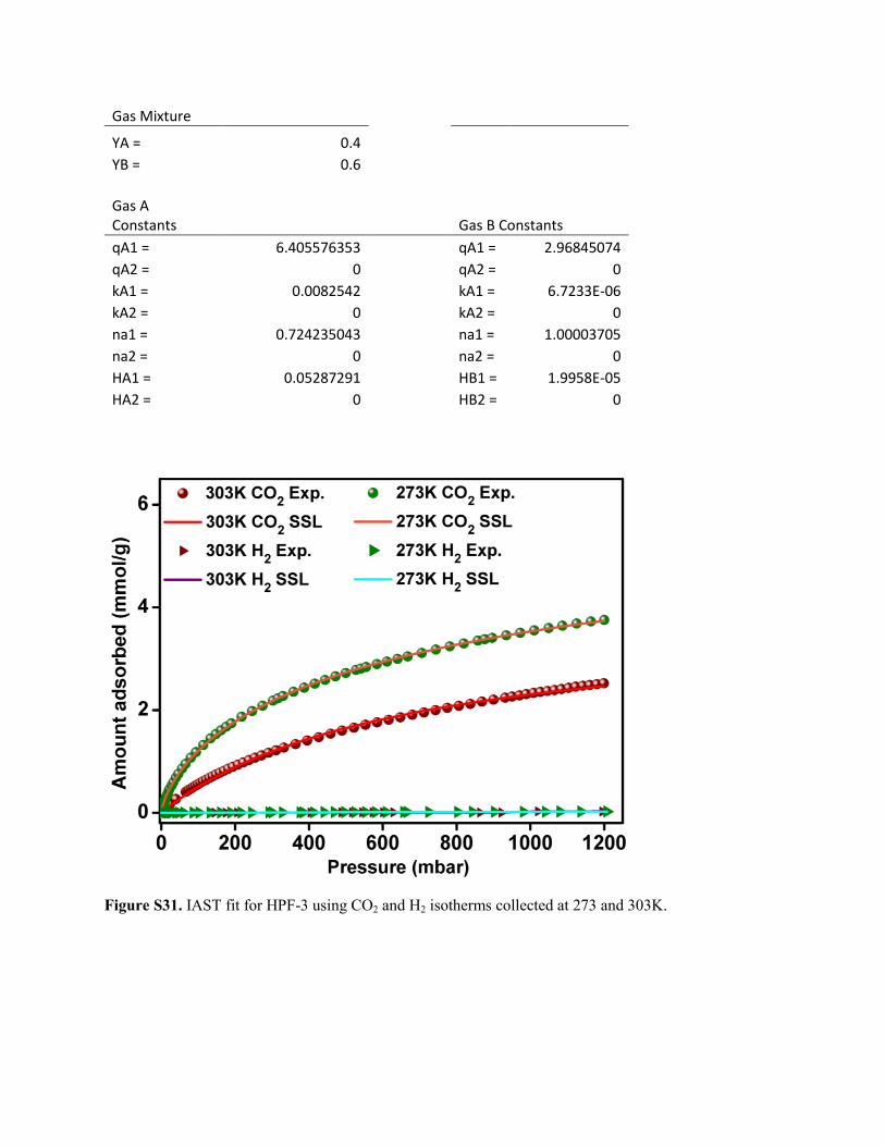
Figure S31. IAST fit for HPF-3 using CO2 and H2 isotherms collected at 273 and 303K.
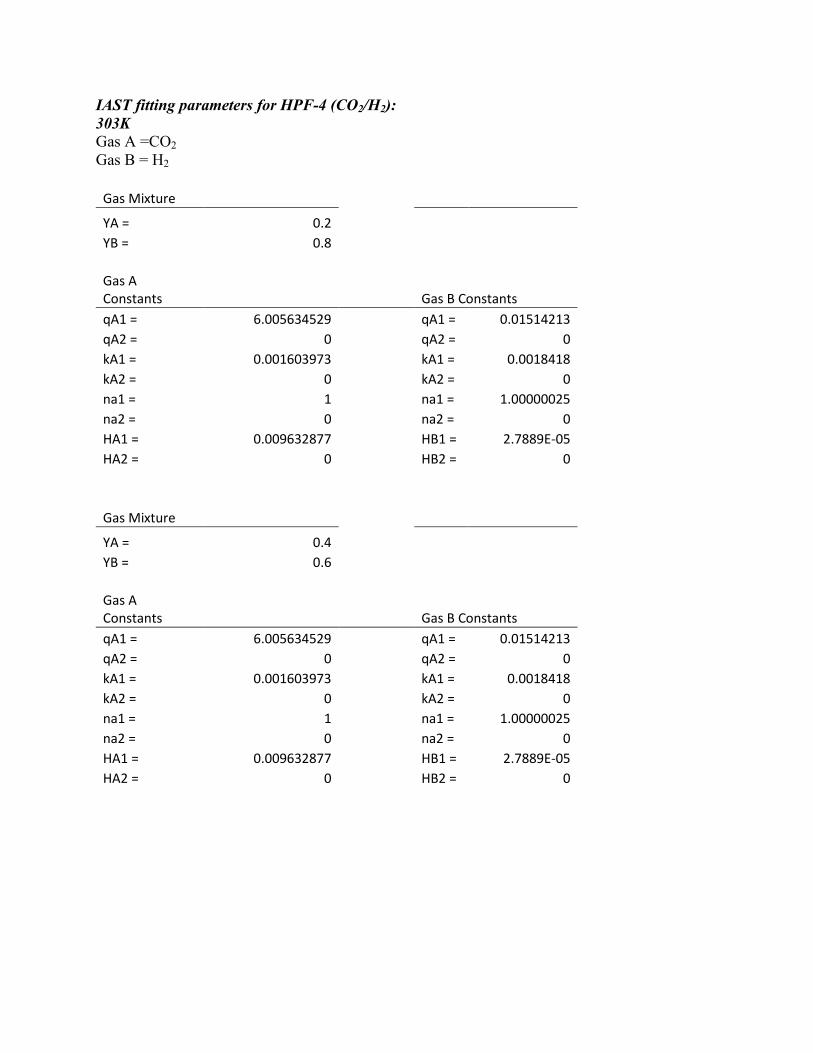
IAST fitting parameters for HPF-4 (CO2/H2):
303K
Gas A =CO2
Gas B = H2
Gas Mixture YA = 0.2 YB = 0.8
Gas A Constants Gas B Constants
qA1 = 6.005634529
qA1 = 0.01514213 qA2 = 0
qA2 = 0
kA1 = 0.001603973
kA1 = 0.0018418 kA2 = 0
kA2 = 0
na1 = 1
na1 = 1.00000025 na2 = 0
na2 = 0
HA1 = 0.009632877
HB1 = 2.7889E-05 HA2 = 0
HB2 = 0
Gas Mixture YA = 0.4 YB = 0.6
Gas A Constants Gas B Constants
qA1 = 6.005634529
qA1 = 0.01514213 qA2 = 0
qA2 = 0
kA1 = 0.001603973
kA1 = 0.0018418 kA2 = 0
kA2 = 0
na1 = 1
na1 = 1.00000025 na2 = 0
na2 = 0
HA1 = 0.009632877
HB1 = 2.7889E-05 HA2 = 0
HB2 = 0
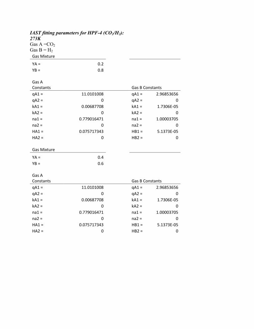
IAST fitting parameters for HPF-4 (CO2/H2):
273K
Gas A =CO2
Gas B = H2
Gas Mixture YA = 0.2 YB = 0.8
Gas A Constants Gas B Constants
qA1 = 11.0101008
qA1 = 2.96853656 qA2 = 0
qA2 = 0
kA1 = 0.00687708
kA1 = 1.7306E-05 kA2 = 0
kA2 = 0
na1 = 0.779016471
na1 = 1.00003705 na2 = 0
na2 = 0
HA1 = 0.075717343
HB1 = 5.1373E-05 HA2 = 0
HB2 = 0
Gas Mixture YA = 0.4 YB = 0.6
Gas A Constants Gas B Constants
qA1 = 11.0101008
qA1 = 2.96853656 qA2 = 0
qA2 = 0
kA1 = 0.00687708
kA1 = 1.7306E-05 kA2 = 0
kA2 = 0
na1 = 0.779016471
na1 = 1.00003705 na2 = 0
na2 = 0
HA1 = 0.075717343
HB1 = 5.1373E-05 HA2 = 0
HB2 = 0
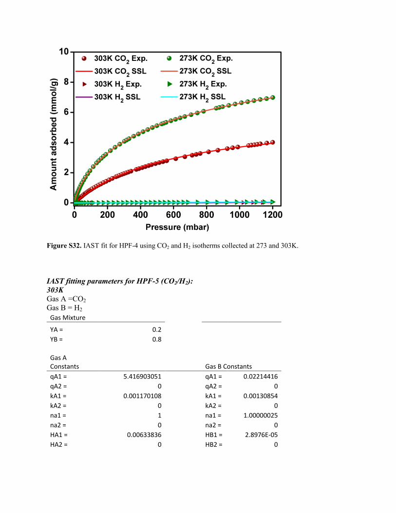
Figure S32. IAST fit for HPF-4 using CO2 and H2 isotherms collected at 273 and 303K.
IAST fitting parameters for HPF-5 (CO2/H2):
303K
Gas A =CO2
Gas B = H2
Gas Mixture YA = 0.2 YB = 0.8
Gas A Constants Gas B Constants
qA1 = 5.416903051
qA1 = 0.02214416 qA2 = 0
qA2 = 0
kA1 = 0.001170108
kA1 = 0.00130854 kA2 = 0
kA2 = 0
na1 = 1
na1 = 1.00000025 na2 = 0
na2 = 0
HA1 = 0.00633836
HB1 = 2.8976E-05 HA2 = 0
HB2 = 0

Gas Mixture YA = 0.4 YB = 0.6
Gas A Constants Gas B Constants
qA1 = 5.416903051
qA1 = 0.02214416 qA2 = 0
qA2 = 0
kA1 = 0.001170108
kA1 = 0.00130854 kA2 = 0
kA2 = 0
na1 = 1
na1 = 1.00000025 na2 = 0
na2 = 0
HA1 = 0.00633836
HB1 = 2.8976E-05 HA2 = 0
HB2 = 0
IAST fitting parameters for HPF-5 (CO2/H2):
273K
Gas A =CO2
Gas B = H2
Gas Mixture YA = 0.2 YB = 0.8
Gas A Constants Gas B Constants
qA1 = 8.596375223
qA1 = 2.96854993
qA2 = 0
qA2 = 0 kA1 = 0.00529283
kA1 = 1.5007E-05
kA2 = 0
kA2 = 0 na1 = 0.801439785
na1 = 1.00003705
na2 = 0
na2 = 0 HA1 = 0.045499155
HB1 = 4.4548E-05
HA2 = 0
HB2 = 0
Gas Mixture YA = 0.4 YB = 0.6
Gas A Constants Gas B Constants
qA1 = 8.596375223
qA1 = 2.96854993 qA2 = 0
qA2 = 0
kA1 = 0.00529283
kA1 = 1.5007E-05 kA2 = 0
kA2 = 0
na1 = 0.801439785
na1 = 1.00003705
na2 = 0
na2 = 0 HA1 = 0.045499155
HB1 = 4.4548E-05
HA2 = 0
HB2 = 0
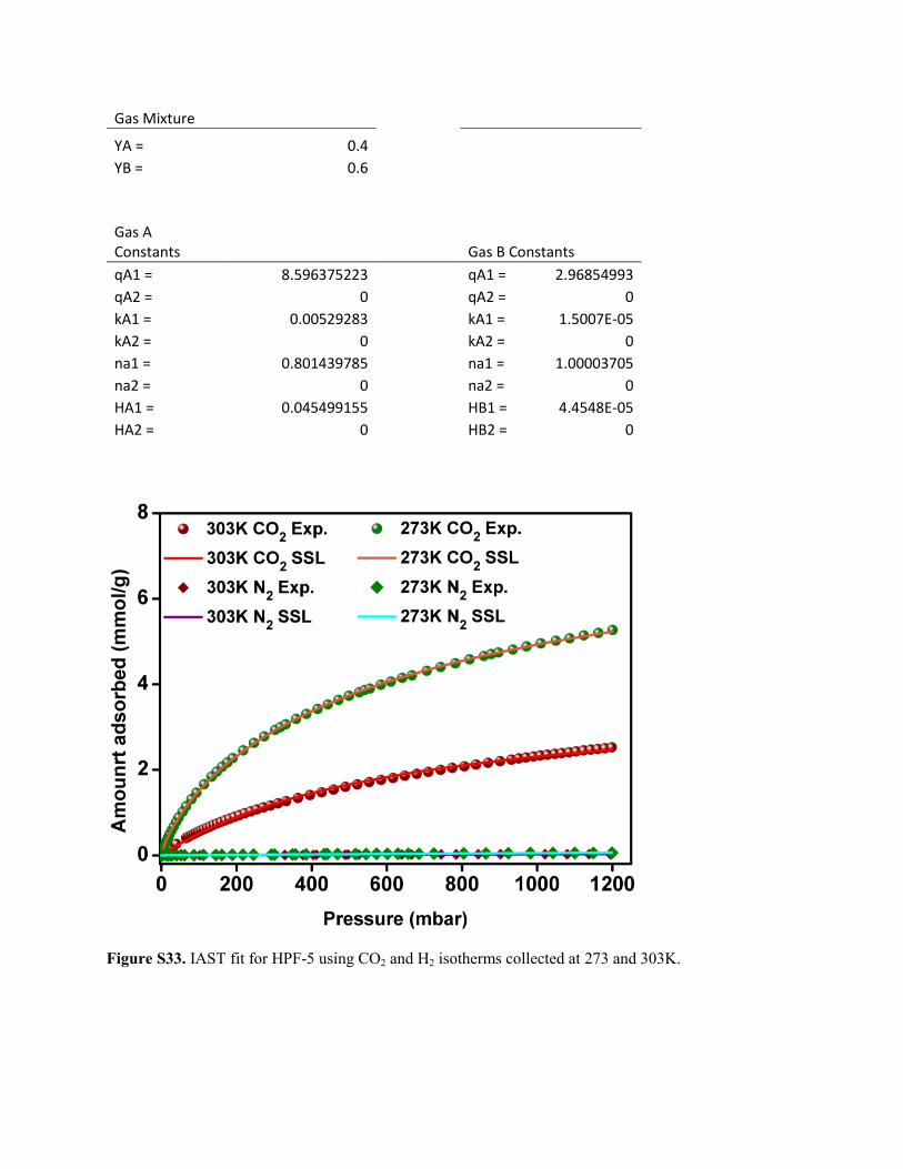
Figure S33. IAST fit for HPF-5 using CO2 and H2 isotherms collected at 273 and 303K.
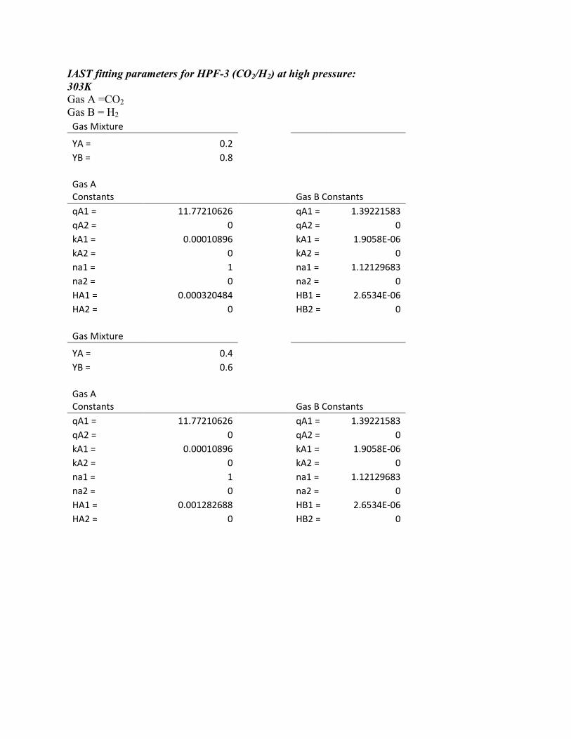
IAST fitting parameters for HPF-3 (CO2/H2) at high pressure:
303K
Gas A =CO2
Gas B = H2
Gas Mixture YA = 0.2 YB = 0.8
Gas A Constants Gas B Constants
qA1 = 11.77210626
qA1 = 1.39221583 qA2 = 0
qA2 = 0
kA1 = 0.00010896
kA1 = 1.9058E-06 kA2 = 0
kA2 = 0
na1 = 1
na1 = 1.12129683 na2 = 0
na2 = 0
HA1 = 0.000320484
HB1 = 2.6534E-06 HA2 = 0
HB2 = 0
Gas Mixture YA = 0.4 YB = 0.6
Gas A Constants Gas B Constants
qA1 = 11.77210626
qA1 = 1.39221583 qA2 = 0
qA2 = 0
kA1 = 0.00010896
kA1 = 1.9058E-06 kA2 = 0
kA2 = 0
na1 = 1
na1 = 1.12129683 na2 = 0
na2 = 0
HA1 = 0.001282688
HB1 = 2.6534E-06 HA2 = 0
HB2 = 0
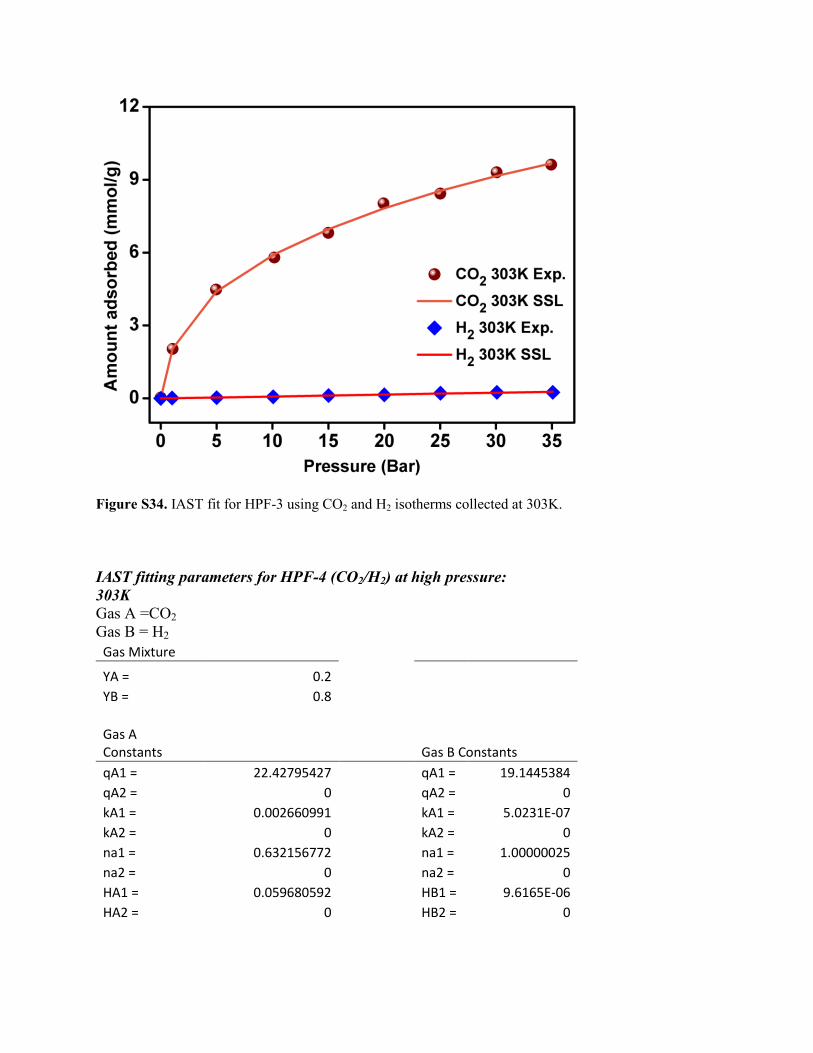
Figure S34. IAST fit for HPF-3 using CO2 and H2 isotherms collected at 303K.
IAST fitting parameters for HPF-4 (CO2/H2) at high pressure:
303K
Gas A =CO2
Gas B = H2
Gas Mixture YA = 0.2 YB = 0.8
Gas A Constants Gas B Constants
qA1 = 22.42795427
qA1 = 19.1445384 qA2 = 0
qA2 = 0
kA1 = 0.002660991
kA1 = 5.0231E-07 kA2 = 0
kA2 = 0
na1 = 0.632156772
na1 = 1.00000025 na2 = 0
na2 = 0
HA1 = 0.059680592
HB1 = 9.6165E-06 HA2 = 0
HB2 = 0

Gas Mixture YA = 0.4 YB = 0.6
Gas A Constants Gas B Constants
qA1 = 22.42795427
qA1 = 19.1445384 qA2 = 0
qA2 = 0
kA1 = 0.002660991
kA1 = 5.0231E-07 kA2 = 0
kA2 = 0
na1 = 0.632156772
na1 = 1.00000025 na2 = 0
na2 = 0
HA1 = 0.059680592
HB1 = 9.6165E-06 HA2 = 0
HB2 = 0
Figure S35. IAST fit for HPF-4 using CO2 and H2 isotherms collected at 303K.
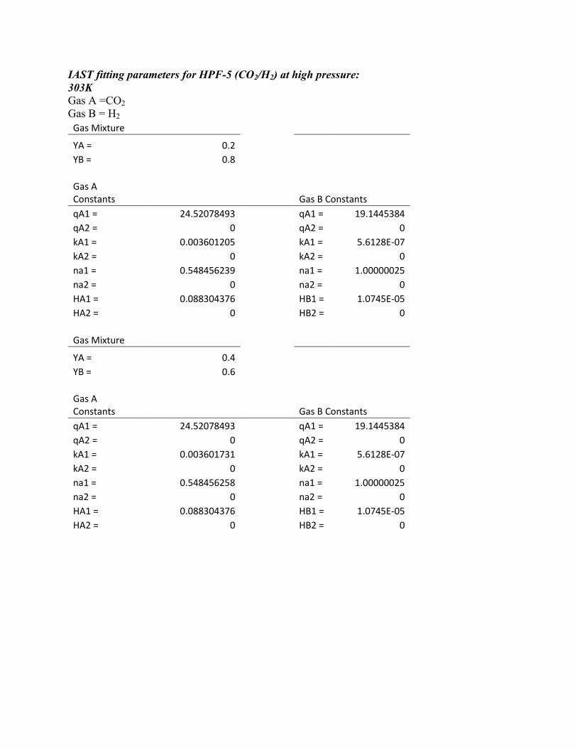
IAST fitting parameters for HPF-5 (CO2/H2) at high pressure:
303K
Gas A =CO2
Gas B = H2
Gas Mixture YA = 0.2 YB = 0.8
Gas A Constants Gas B Constants
qA1 = 24.52078493
qA1 = 19.1445384 qA2 = 0
qA2 = 0
kA1 = 0.003601205
kA1 = 5.6128E-07 kA2 = 0
kA2 = 0
na1 = 0.548456239
na1 = 1.00000025 na2 = 0
na2 = 0
HA1 = 0.088304376
HB1 = 1.0745E-05 HA2 = 0
HB2 = 0
Gas Mixture YA = 0.4 YB = 0.6
Gas A Constants Gas B Constants
qA1 = 24.52078493
qA1 = 19.1445384 qA2 = 0
qA2 = 0
kA1 = 0.003601731
kA1 = 5.6128E-07 kA2 = 0
kA2 = 0
na1 = 0.548456258
na1 = 1.00000025 na2 = 0
na2 = 0
HA1 = 0.088304376
HB1 = 1.0745E-05 HA2 = 0
HB2 = 0

Figure S36. IAST fit for HPF-5 using CO2 and H2 isotherms collected at 303K.
6. Contact angle measurement:
Contact angles were measured on the polymers surfaces using computerized camera
technique and processed with ImageJ software.
For the measurement the polymer powder was spreaded homogeniously on the glass
slide. Then droplet of water slowly placed on the top of the polymer surface with a syringe
needle. The camera was focused to the particular region and images were recorded. Note: The
surface hydrophobicity of the sample is sensitive to the reaction condition and this is because of
the texture of the final product. However, the intrinsic hydrophobicity remains the same even
when the synthesis conditions (time 3 days vs. 4 days, or solvent amounts) are varied. This is
confirmed from the solvent sorption experiments.
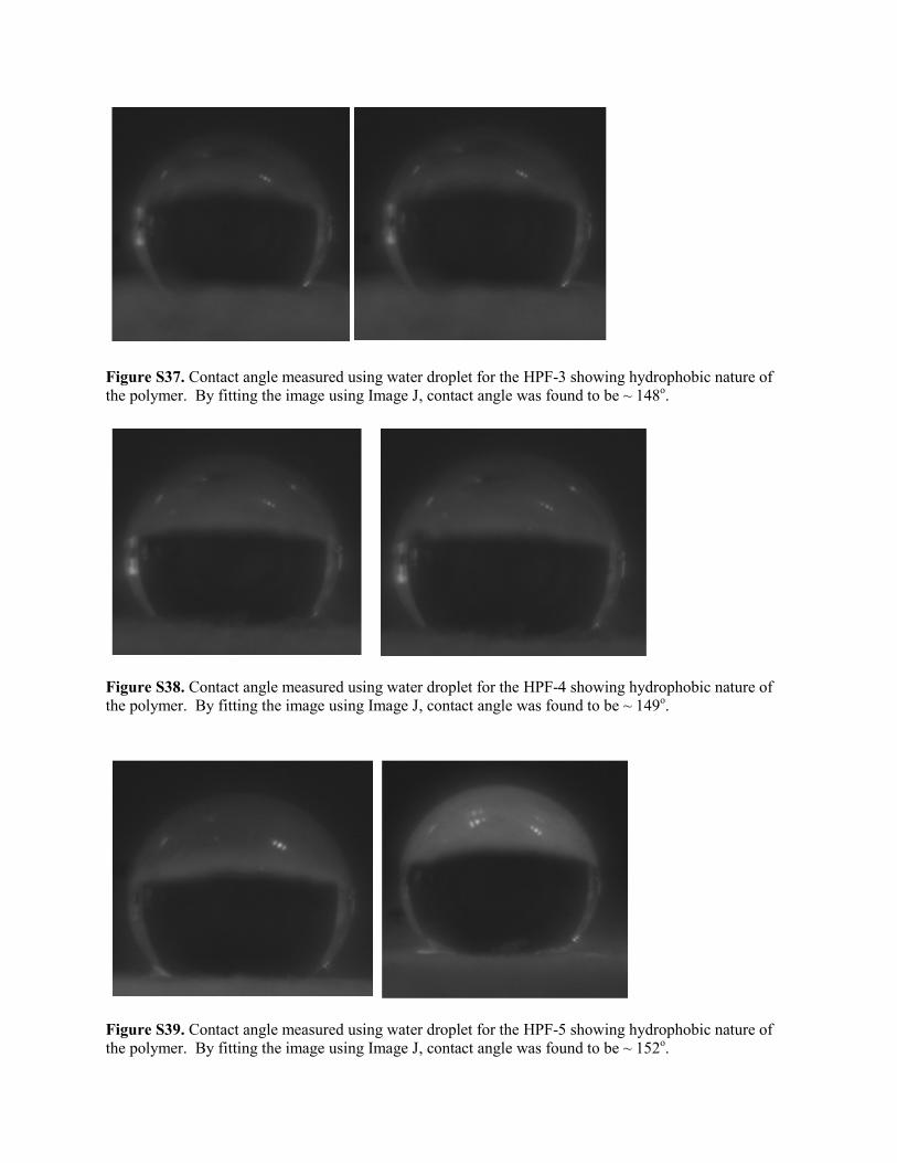
Figure S37. Contact angle measured using water droplet for the HPF-3 showing hydrophobic nature of
the polymer. By fitting the image using Image J, contact angle was found to be ~ 148o.
Figure S38. Contact angle measured using water droplet for the HPF-4 showing hydrophobic nature of
the polymer. By fitting the image using Image J, contact angle was found to be ~ 149o.
Figure S39. Contact angle measured using water droplet for the HPF-5 showing hydrophobic nature of
the polymer. By fitting the image using Image J, contact angle was found to be ~ 152o.
7. TGA Cycling Experiment:
For the cycling experiments, no protective gas was used, and the gas flows were
systematically switched between CO2 and He on the purge lines. The methanol exchanged and
activated (150oC, 6 hrs) sample of HPF-3, HPF-4 and HPF-5 were loaded on to the Pt pans and
evacuated for 6hrs prior to the runs. TGA and DSC calibration and corrections runs were done
prior to carrying out the cycling experiments.
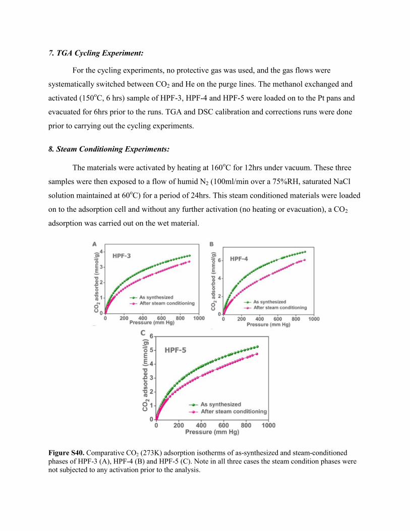
8. Steam Conditioning Experiments:
The materials were activated by heating at 160oC for 12hrs under vacuum. These three
samples were then exposed to a flow of humid N2 (100ml/min over a 75%RH, saturated NaCl
solution maintained at 60oC) for a period of 24hrs. This steam conditioned materials were loaded
on to the adsorption cell and without any further activation (no heating or evacuation), a CO2
adsorption was carried out on the wet material.
Figure S40. Comparative CO2 (273K) adsorption isotherms of as-synthesized and steam-conditioned
phases of HPF-3 (A), HPF-4 (B) and HPF-5 (C). Note in all three cases the steam condition phases were
not subjected to any activation prior to the analysis.
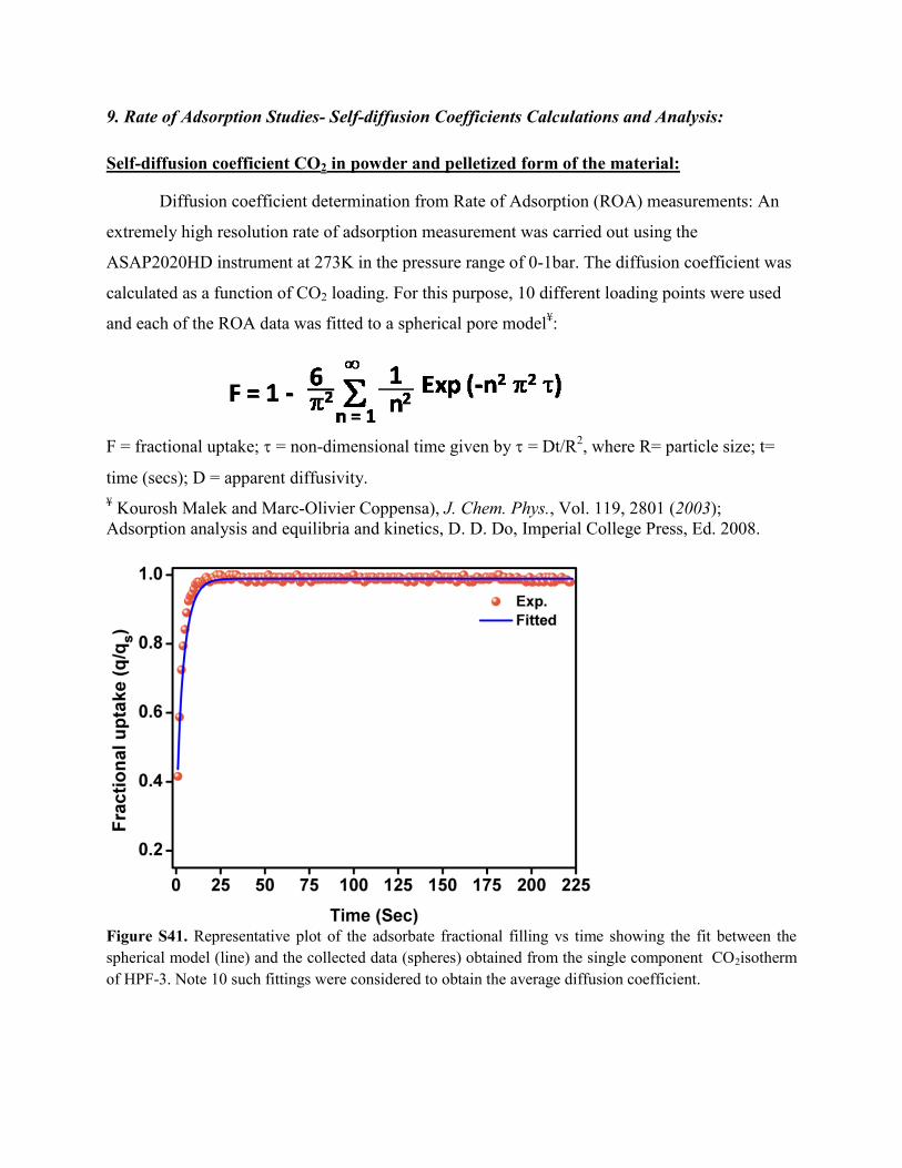
9. Rate of Adsorption Studies- Self-diffusion Coefficients Calculations and Analysis:
Self-diffusion coefficient CO2 in powder and pelletized form of the material:
Diffusion coefficient determination from Rate of Adsorption (ROA) measurements: An
extremely high resolution rate of adsorption measurement was carried out using the
ASAP2020HD instrument at 273K in the pressure range of 0-1bar. The diffusion coefficient was
calculated as a function of CO2 loading. For this purpose, 10 different loading points were used
and each of the ROA data was fitted to a spherical pore model¥:
F = fractional uptake; = non-dimensional time given by = Dt/R
2, where R= particle size; t=
time (secs); D = apparent diffusivity.
¥ Kourosh Malek and Marc-Olivier Coppensa), J. Chem. Phys., Vol. 119, 2801 (2003);
Adsorption analysis and equilibria and kinetics, D. D. Do, Imperial College Press, Ed. 2008.
Figure S41. Representative plot of the adsorbate fractional filling vs time showing the fit between the
spherical model (line) and the collected data (spheres) obtained from the single component CO2isotherm
of HPF-3. Note 10 such fittings were considered to obtain the average diffusion coefficient.

Figure S42. Representative plot of the adsorbate fractional filling vs time showing the fit between the
spherical model (line) and the collected data (spheres) obtained from the single component CO2 isotherm
of HPF-4. Note 10 such fittings were considered to obtain the average diffusion coefficient.
Figure S43. A plot of the adsorbate fractional filling vs time showing the fit between the spherical model
(line) and the collected data (spheres) obtained from the single component CO2 isotherm of HPF-5. Note
10 such fittings were considered to obtain the average diffusion coefficient.
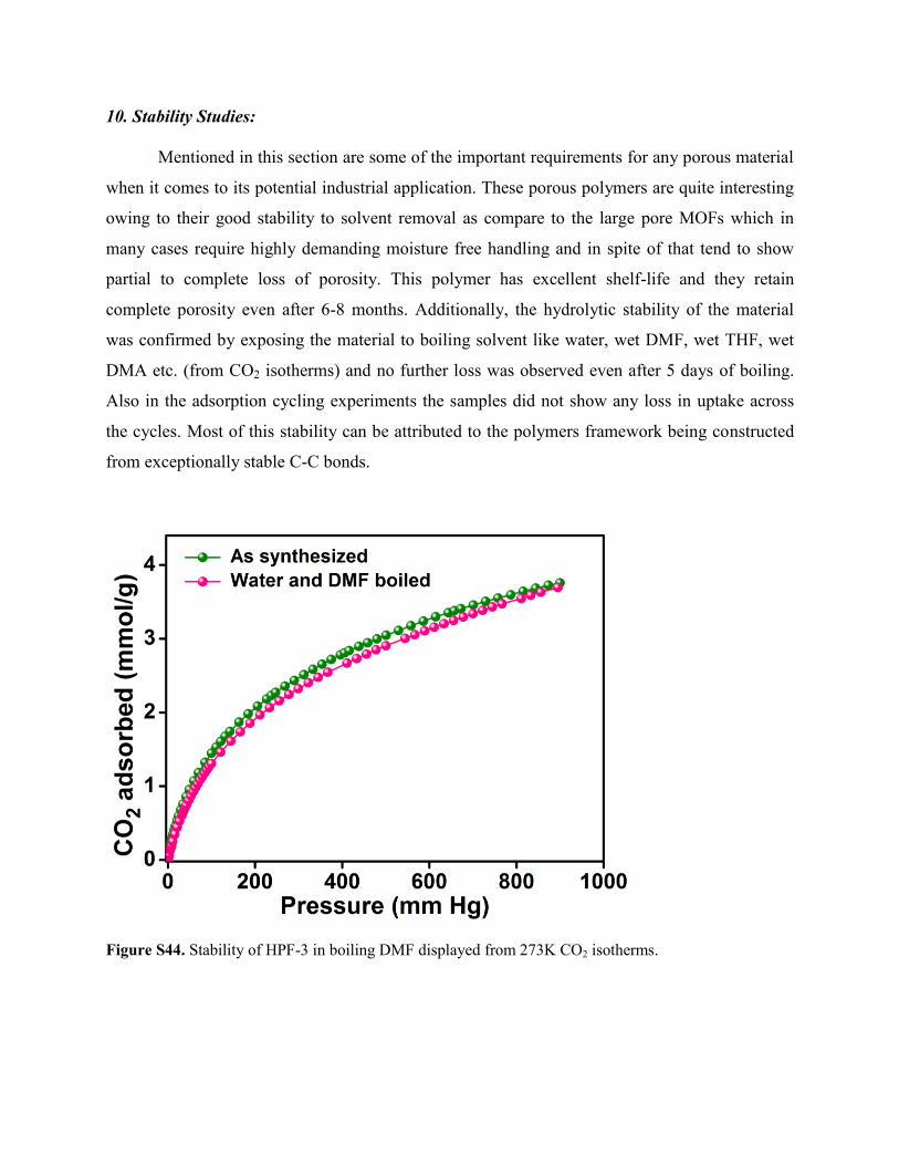
10. Stability Studies:
Mentioned in this section are some of the important requirements for any porous material
when it comes to its potential industrial application. These porous polymers are quite interesting
owing to their good stability to solvent removal as compare to the large pore MOFs which in
many cases require highly demanding moisture free handling and in spite of that tend to show
partial to complete loss of porosity. This polymer has excellent shelf-life and they retain
complete porosity even after 6-8 months. Additionally, the hydrolytic stability of the material
was confirmed by exposing the material to boiling solvent like water, wet DMF, wet THF, wet
DMA etc. (from CO2 isotherms) and no further loss was observed even after 5 days of boiling.
Also in the adsorption cycling experiments the samples did not show any loss in uptake across
the cycles. Most of this stability can be attributed to the polymers framework being constructed
from exceptionally stable C-C bonds.
Figure S44. Stability of HPF-3 in boiling DMF displayed from 273K CO2 isotherms.
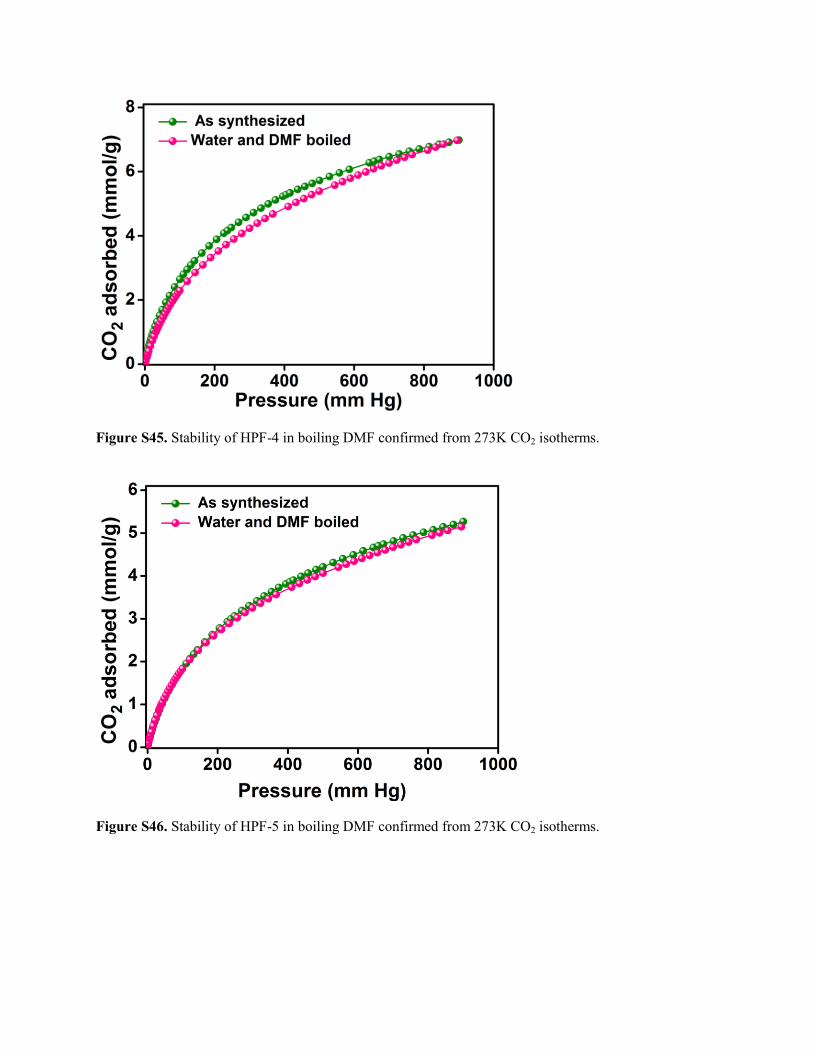
Figure S45. Stability of HPF-4 in boiling DMF confirmed from 273K CO2 isotherms.
Figure S46. Stability of HPF-5 in boiling DMF confirmed from 273K CO2 isotherms.

Acid stability study: about 250 mg of each polymer was dispersed in 3ml of H2O and 0.5 ml of
MeOH were taken in three different small vials. In three different bigger vials a mixture of
ClSO3H (2ml) and HNO3 (2ml) was taken. Now the smaller vials containing the dispersions of
different polymers were kept inside the bigger vials and screw capped in such a way that enough
of acidic vapours goes in to the smaller vials but the acid did not directly touch the polymers.
These vial-in-a-vial set-ups were placed at ~50oC. After 6 hrs the smaller vials containing the
polymers were taken out and pH of the solution was found to be in between 2 to 2.5. The
polymer samples were filtered and washed thoroughly with water, methanol and finally with
plenty of THF. These polymers were then dried under vacuum and used for gas adsorption
analysis. Only <2% drops in CO2 capacity was observed in each case after this treatment.
Figure S47. Comparison of the pore sizes between the as-made and the acid treated samples. Note: The
pore sizes are estimated from the 273K CO2 adsorption isotherms.

Stability of the pelletized material: About 250 mg of powder HPF-4 was subjected to 15 ton of
pressure for 30 minutes using a hydraulic pelletizer. After that the pellet was subjected to pre
treatment prior to gas adsorption under similar conditions employed for the powder samples. The
thickness of the pellet before and after gas adsorption remains unchanged (Figures S48). This
lack of swolling in a polymer is highly desirable for practical gas separation applications.
Figure S48. (A) Photographic image of HPF-4 in powder and pellet form. Thickness of the pellet before
(B) and after(C) the adsorption study.
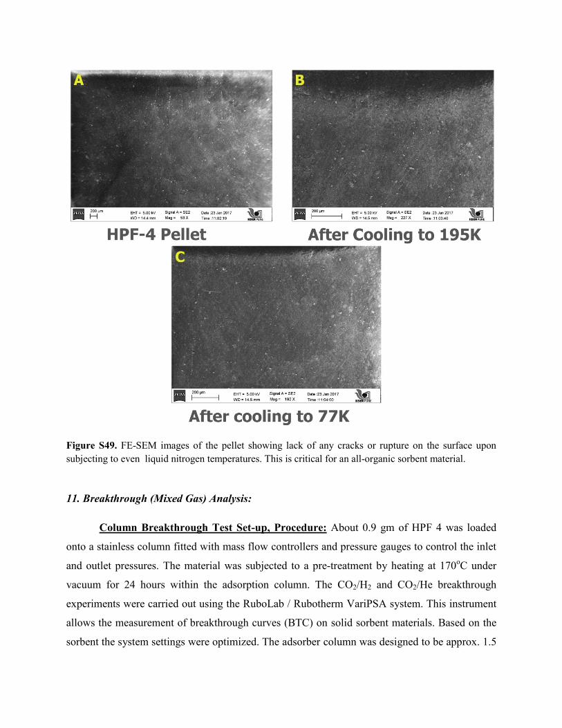
Figure S49. FE-SEM images of the pellet showing lack of any cracks or rupture on the surface upon
subjecting to even liquid nitrogen temperatures. This is critical for an all-organic sorbent material.
11. Breakthrough (Mixed Gas) Analysis:
Column Breakthrough Test Set-up, Procedure: About 0.9 gm of HPF 4 was loaded
onto a stainless column fitted with mass flow controllers and pressure gauges to control the inlet
and outlet pressures. The material was subjected to a pre-treatment by heating at 170oC under
vacuum for 24 hours within the adsorption column. The CO2/H2 and CO2/He breakthrough
experiments were carried out using the RuboLab / Rubotherm VariPSA system. This instrument
allows the measurement of breakthrough curves (BTC) on solid sorbent materials. Based on the
sorbent the system settings were optimized. The adsorber column was designed to be approx. 1.5
ml in volume. To measure the sorption based temperature (adsorption front), three temperature
sensors were integrated to measure the temperature at two/three different positions within the
adsorber bed. (Thermocouple type K, 3 mm diameter of temperature sensor). The gas flow
across the column was controlled using a micro-metering valve. All measurements were
performed by using a gas flow of 50 or 100 ml/min. While the adsorption of CO2 was indicated
by its retention time on the column, the complete breakthrough of CO2 was indicated by the
downstream gas composition reaching that of the feed gas. Using the formula,
Number of mole adsorbed, n = F * Ci * t,
Where F = molar flow, Ci = concentration of ith
component and t = retention time.
The CO2 uptake was calculated to be 2.48mmol/g for the 20CO2/80He mixture and this
uptake closely matched with the uptake obtained for the 20CO2/80H2 (2.42 mmol/g) mixture.
This suggest almost negligible amount of H2 is being adsorbed by the polymer. Similarly CO2
uptake was calculated to be 3.52 mmol/g for 40CO2/60H2 mixture.
12. Computational and Molecular Modelling Details:
Structure solution: In our study HPF-4 is the best performing one. We considered only HPF-4
for all the simulation studies. For structure solution we have adopted our earlier reported
strategies.(ref. 50 maintext) In the first step, we created few small oligomers of different length
by combining the monomers in a 2:3 ratio and minimized its structure using DFT methods
(CASTEP routine) with Materials Studio. Random polymerization of these oligomers yielded
longer linear oligomer. These polymers took different configurations depending on the small
differences in the geometry of the initial energy minimized smaller oligomers. Three low energy
oligomers were chosen based on the energy. These oligomers were then polymerized randomly
with branch point at different parts of them. With the lowest energy conformer, amorphous cell
was constructed.
Again this amorphous cell was energy and geometry optimized using the tight-binding DFT
methods (DFT-TB). This yielded a structure with a triclinic unit cell: P1; a = 48.7804A, b
=49.8932A, c = 47.0560A, α = 89.2961 (2)º; β = 90.3408 (4)º, and γ = 90.8990 (4)º. During the
entire process complete rotational and torsional freedom was maintained.
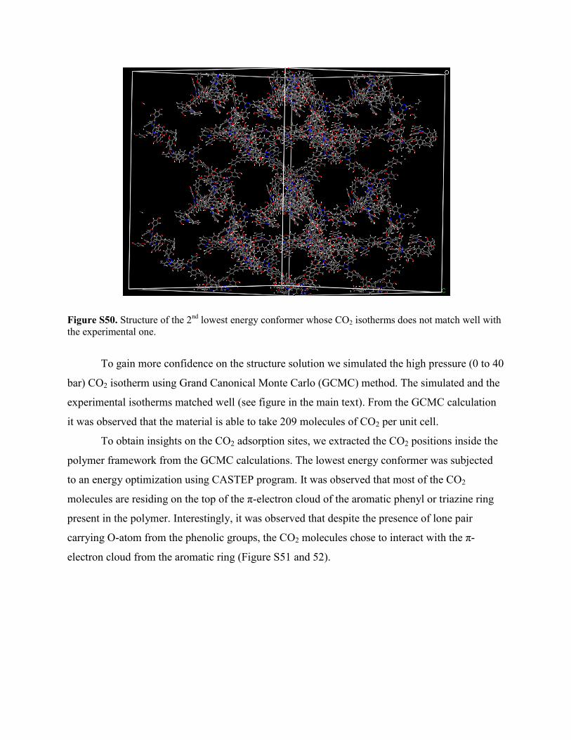
Figure S50. Structure of the 2nd
lowest energy conformer whose CO2 isotherms does not match well with
the experimental one.
To gain more confidence on the structure solution we simulated the high pressure (0 to 40
bar) CO2 isotherm using Grand Canonical Monte Carlo (GCMC) method. The simulated and the
experimental isotherms matched well (see figure in the main text). From the GCMC calculation
it was observed that the material is able to take 209 molecules of CO2 per unit cell.
To obtain insights on the CO2 adsorption sites, we extracted the CO2 positions inside the
polymer framework from the GCMC calculations. The lowest energy conformer was subjected
to an energy optimization using CASTEP program. It was observed that most of the CO2
molecules are residing on the top of the π-electron cloud of the aromatic phenyl or triazine ring
present in the polymer. Interestingly, it was observed that despite the presence of lone pair
carrying O-atom from the phenolic groups, the CO2 molecules chose to interact with the π-
electron cloud from the aromatic ring (Figure S51 and 52).
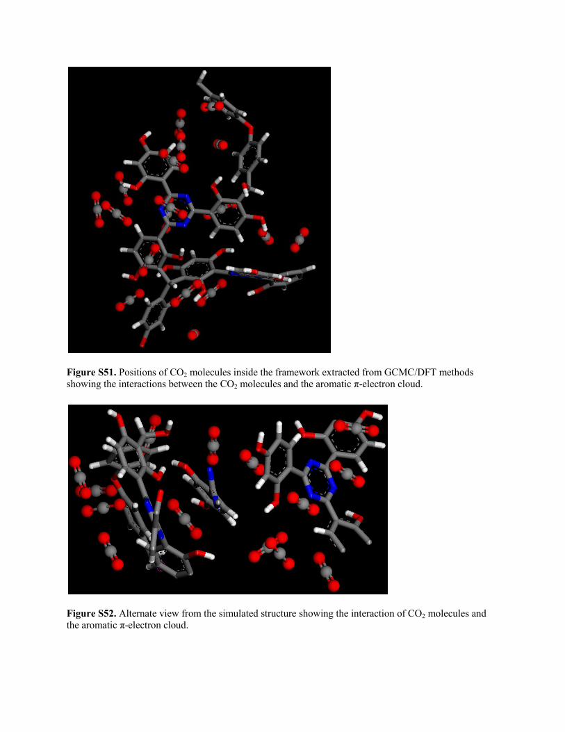
Figure S51. Positions of CO2 molecules inside the framework extracted from GCMC/DFT methods
showing the interactions between the CO2 molecules and the aromatic π-electron cloud.
Figure S52. Alternate view from the simulated structure showing the interaction of CO2 molecules and
the aromatic π-electron cloud.