examining the relationship between teacher preparation
TRANSCRIPT

Georgia State University Georgia State University
ScholarWorks @ Georgia State University ScholarWorks @ Georgia State University
Educational Policy Studies Dissertations Department of Educational Policy Studies
Spring 5-17-2019
Examining the Relationship Between Teacher Preparation Examining the Relationship Between Teacher Preparation
Program Quality and Beginning Teacher Retention Program Quality and Beginning Teacher Retention
Brittany Cunningham
Follow this and additional works at: https://scholarworks.gsu.edu/eps_diss
Recommended Citation Recommended Citation Cunningham, Brittany, "Examining the Relationship Between Teacher Preparation Program Quality and Beginning Teacher Retention." Dissertation, Georgia State University, 2019. https://scholarworks.gsu.edu/eps_diss/204
This Dissertation is brought to you for free and open access by the Department of Educational Policy Studies at ScholarWorks @ Georgia State University. It has been accepted for inclusion in Educational Policy Studies Dissertations by an authorized administrator of ScholarWorks @ Georgia State University. For more information, please contact [email protected].

ACCEPTANCE
This dissertation, EXAMINING THE RELATIONSHIP BETWEEN TEACHER
PREPARATION PROGRAMS AND BEGINNING TEACHER RETENTION, by BRITTANY
CUNNINGHAM, was prepared under the direction of the candidate’s Dissertation Advisory
Committee. It is accepted by the committee members in partial fulfillment of the requirements
for the degree, Doctor of Philosophy, in the College of Education & Human Development,
Georgia State University.
The Dissertation Advisory Committee and the student’s Department Chairperson, as
representatives of the faculty, certify that this dissertation has met all standards of excellence and
scholarship as determined by the faculty. The Dean of the College of Education & Human
Development concurs.
__________________________________
William Curlette, Ph.D.
Committee Chair
__________________________________ __________________________________
Chris Oshima, Ph.D. Hongli Li, Ph.D.
Committee Member Committee Member
__________________________________
Robert Hendrick, Ph.D.
Committee Member
__________________________________
Date
__________________________________
William Curlette, Ph.D.
Chairperson, Department of Educational Policy Studies
__________________________________
Paul Alberto, Ph.D.
Dean, College of Education & Human Development

AUTHOR’S STATEMENT
By presenting this dissertation as partial fulfillment of the requirements for the advanced degree
from Georgia State University, I agree that the library of Georgia State University shall make it
available for inspection and circulation in accordance with its regulations governing materials of
this type. I agree that permission to quote, copy from, or to publish this dissertation may be
granted by professor under whose direction it was written, by the College of Education and
Human Development’s Director of Graduate Studies, or by me. Such quoting, copying, or
publishing that any copying from or publication of this dissertation which involves potential
financial gain will not be allowed without my written permission.
_______________________________________
Brittany Cunningham

NOTICE TO BORROWERS
All dissertations deposited in the Georgia State University library must be used in accordance with
the stipulations prescribed by the author in the preceding statement. The author of this dissertation
is:
Brittany Nichole Cunningham
PO Box 33842
Decatur, GA 30033
The director of this dissertation is:
William Curlette, Ph.D.
Department of Educational Policy Studies
College of Education & Human Development
Georgia State University
Atlanta, GA 30303

CURRICULUM VITAE
Brittany Cunningham
ADDRESS: PO Box 33842
Decatur, GA 30033
EDUCATION:
Ph.D. 2019 Georgia State University
Educational Policy Studies
M.S. 2003 Georgia State University
Managerial Sciences
B.B.A. 1997 Emory University
Accounting and Finance
PROFESSIONAL EXPERIENCE:
2017-present Director, Testing + Assessment
Atlanta Public Schools
2013-2017 Principal, Druid Hills High School
DeKalb County School District
2009-2013 Principal, Sequoyah Middle School
DeKalb County School District
2006-2009 Assistant Principal, Sequoyah Middle
DeKalb County School District
2004-2006 Teacher, Sequoyah Middle School
DeKalb County School District
2001-2004 Teacher, River Trail Middle School
Fulton County School District
1999-2001 Teacher, Cole Visual and Performing Arts
Oakland Unified School District
1997-1999 Treasury and Risk Management Analyst
Hitachi Data Systems

PRESENTATIONS AND PUBLICATIONS
Cunningham, Brittany, Nunez, Sandra, & Hall, Evelyn. (2009, September). A passion for
English language learners: An administrator’s perspective. For presentation at Southeast
Regional TESOL Conference, Atlanta, GA.
Cunningham, Brittany & Duckett, Skye. (2018, September). APS moving forward through
prevention, practice, and policy. For presentation at Georgia Professional Standards
Commission Ethics Symposium, Macon, Georgia.
Cunningham, Brittany & Duckett, Skye. (2018, October). APS moving forward through
prevention, practice, and policy. For presentation at National Association of State Directors of
Teacher Education and Certification Professional Practices Institute, Portland, Maine.
PROFESSIONAL SOCIETIES AND ORGANIZATIONS
2003-present Beta Gamma Sigma
2008-present American Educational Research Association
2011-present Pi Lambda Theta
2018-present Georgia Association of Educational Leaders
2019-present Georgia Assessment and Accountability Professionals

EXAMINING THE RELATIONSHIP BETWEEN TEACHER PREPARATION PROGRAM
QUALITY AND BEGINNING TEACHER RETENTION
by
BRITTANY CUNNINGHAM
Under the Direction of Dr. William Curlette
ABSTRACT
In order to provide equal access to a high-quality education that prepares students for
global competitiveness, local education agencies are constantly working to recruit bright new
educators and engage in practices that support teacher development and retention. The purpose
of this study is to examine how teacher preparation program quality and the impact of various
individual and school-level characteristics relate to beginning teacher attrition. Propensity score
matching, specifically optimal full matching, was used to match teachers who participated in two
post-baccalaureate teacher preparation programs with year-long residencies on eight variables.
The study supported the hypothesis that program participants had significantly higher average
treatment effect and average treatment effect of the treated, indicating higher one- and five-year
retention rates than non-participants who began teaching the same school year. The average
treatment effect models had a moderate effect size, with the year five average treatment effect of
the treated model having a small effect size. The significant findings may indicate that the

signature components of CREST-Ed and Net-Q programs, such as the year-long residency and
TIP-AAR, have a long-term impact on teacher quality. Results of the multilevel logistic
regression and average treatment effect models confirmed that factors such as teacher age,
teacher race/ethnicity, school socioeconomic composition, school performance and subject
taught were significant predictors of teacher retention. However, teacher race/ethnicity was the
only significant variable found in all average treatment effect models, suggesting that the factors
influencing teacher retention are dynamic over time and change as teachers gain classroom
experience. The study contributes to scholarly knowledge in the design of teacher residency
programs and on factors associated with beginning teacher retention. The findings from this
study may assist local education agencies and educator preparation providers in understanding
ways to support pre-service and beginning teachers. Suggestions for future research and
implications for policies addressing pre-service teacher support and teacher retention are
discussed.
INDEX WORDS: teacher attrition, pre-service teacher residencies, propensity score matching

EXAMINING THE RELATIONSHIP BETWEEN TEACHER PREPARATION PROGRAM
QUALITY AND BEGINNING TEACHER RETENTION
by
BRITTANY CUNNINGHAM
A Dissertation
Presented in Partial Fulfillment of Requirements for the
Degree of
Doctor of Philosophy
in
Educational Policy Studies
in
Research, Measurement, and Statistics
in
the College of Education & Human Development
Georgia State University
Atlanta, GA
2019

Copyright by
Brittany N. Cunningham
2019

ii
ACKNOWLEGEMENT
First, I must give honor to God, who has carried me through this journey, which proved
to be a lengthy lesson in resilience, patience, and faith. It takes a village to carry a doctoral
student from first day of classes to their hooding ceremony, and I have been blessed beyond
measure to have the support of so many people. A heartfelt thank you goes to all the following:
To my husband, Everett Patrick, who has been a major source of love, encouragement
and support for nine of the years I have been on this doctoral journey.
To my parents, Janet Cunningham, Gerald Cunningham, Sandra Cunningham, and
brother, Phillip Cunningham, who have patiently waited for me to complete this voyage.
Through it all, they knew beyond a shadow of a doubt that somehow, I would find the courage
and strength to finish.
To my parents and siblings through marriage, Dr. James and Ethel Patrick, Mark and
Ursula Carter, Jennifer Cunningham, Elliot Patrick and Dr. Mesha Ramsey-Patrick, many of
whom have served as inspiration through their distinguished service and leadership in K-12
education and/or post-secondary academia.
To my niece, Isabella, nephew, John Phillip, and godson, Warren, whom my desire to
model what I preached was, at times, the only reason I could find to persevere.
To my Dissertation Committee, Dr. William Curlette, Dr. Chris Oshima, Dr. Hongli Li,
and Dr. Robert Hendrick, many of whom I have known for ten years, for their patience,
guidance, feedback, and support.
To my sisters by choice, whose love, laughter, prodding, and tears paved a pathway
throughout this maze: Dr. Kia Billingsley, Venessa Bines-Truitt, Dr. Maria Dixon, Dr. Keisha
Hancock, Termerion Lakes-McCrary, Katrina Massey, Dr. Marguerite McClinton-Stoglin, Sonja
Tobler, Dr. Rosalyn Washington, and Dr. Nakiesha Sprull.
To the members of Sun in My Soul and Summer Vacation Club, all of whom have filled
me with food, fellowship, laughter, support, and a welcome respite from my research.
To my supervisors and team members at DeKalb County School District and Atlanta
Public Schools, all of whom have provided empathy, encouragement, patience, and support
during this trek. There are too many champions to name, but here are the some of my strongest
supporters: Trenton Arnold, Samantha Clay, Beth Heckman, Dr. Tiffany Hogan, Michael
Lamont, Dr. Knox Phillips, Dr. Katelyn Plescow, Dr. Angela Pringle, Dr. Eva Van de Water.
To Dr. Comfort Afolabi, who not only provided key datasets, but also advice,
encouragement, and motivation to finally complete this.
To Dr. Phill Gagne, who took me in as an advisee when I needed one, challenged me to
think big even when I felt insignificant, and took me to task when I could give more of myself.
To Dr. Janice Fournillier, for being a role model and a quiet but steady motivator. In my
times of severe doubt, God always planted you in the EPS hallway to keep me grounded and
focused.
To those I have not formally recognized but deserve appreciation, please charge it to my
head and not my heart.
“Do not judge me by my success, judge me by how many times I fell down and got back
up again.” --Nelson Mandela

iii
TABLE OF CONTENTS
Contents
LIST OF TABLES .......................................................................................................................... iv
LIST OF FIGURES ........................................................................................................................ vi
LIST OF ABBREVIATIONS ........................................................................................................ vii
1 BACKGROUND ...................................................................................................................... 1
Guiding Questions ....................................................................................................................... 1
Review ......................................................................................................................................... 2
Summary .................................................................................................................................... 58
References .................................................................................................................................. 59
2 METHODOLOGY, FINDINGS, AND DISCUSSION .......................................................... 78
Methodology .............................................................................................................................. 78
Results and Discussion .............................................................................................................. 93
Conclusion ............................................................................................................................... 109
References ................................................................................................................................ 116
APPENDICES ............................................................................................................................. 120

iv
LIST OF TABLES
Table Page
1 Percentage distribution of why public school teachers left the profession: 2012-
2013. . . . . . . . . . . . . . . . . . . . . . . . . . . . . . . . . . . . . . . . . . . . . . . . . . . . . . . . . . . .
7
2 Percentage distribution of current occupation status of public school teachers
who left the profession: 2012-2013. . . . . . . . . . . . . . . . . . . . . . . . . . . . . . . . . . . .
7
3 Reasons why first-year teachers left the profession: 2007-2008. . . . . . . . . . . . . 8
4 Percentage distribution of public school teachers with five years or less
teaching experience, by how well prepared they were to handle the following in
the first year of teaching . . . . . . . . . . . . . . . . . . . . . . . . . . . . . . . . . . . . . . . . . . . .
9
5 2018 CCRPI Indicator Weights . . . . . . . . . . . . . . . . . . . . . . . . . . . . . . . . . . . . . . 18
6 SGP Growth Levels . . . . . . . . . . . . . . . . . . . . . . . . . . . . . . . . . . . . . . . . . . . . . . . 19
7 Weighted Suspension Rate . . . . . . . . . . . . . . . . . . . . . . . . . . . . . . . . . . . . . . . . . . 22
8 NCATE Unit Standards . . . . . . . . . . . . . . . . . . . . . . . . . . . . . . . . . . . . . . . . . . . . 24
9 Most important proposals for improving teacher preparation programs . . . . . . . 37
10 Teacher Demographics of Treatment Sample . . . . . . . . . . . . . . . . . . . . . . . . . . . . 82
11 Teacher Demographics of Treatment Sample – Year 1. . . . . . . . . . . . . . . . . . . . . 83
12 Teacher Demographics of Treatment Sample – Year 3. . . . . . . . . . . . . . . . . . . . . 84
13 Teacher Demographics of Treatment Sample – Year 5. . . . . . . . . . . . . . . . . . . . 84
14 Teacher Demographics of Control Sample - Year 1 . . . . . . . . . . . . . . . . . . . . . . . 85
15 Teacher Demographics of Control Sample - Year 3 . . . . . . . . . . . . . . . . . . . . . . . 85
16
17
18
Teacher Demographics of Control Sample - Year 5 . . . . . . . . . . . . . . . . . . . . . . .
Percentage of Retained Teachers . . . . . . . . . . . . . . . . . . . . . . . . . . . . . . . . . . . . .
School Composition . . . . . . . . . . . . . . . . . . . . . . . . . . . . . . . . . . . . . . . . . . . . . . .
86
86
87
19 Missing Data Analysis . . . . . . . . . . . . . . . . . . . . . . . . . . . . . . . . . . . . . . . . . . . . . 89

v
20 Missing Data Analysis Breakdown by Case . . . . . . . . . . . . . . . . . . . . . . . . . . . . . 89
21 Multilevel Logistic Analysis – Year One . . . . . . . . . . . . . . . . . . . . . . . . . . . . . . . 96
22 Multilevel Logistic Analysis – Year Three. . . . . . . . . . . . . . . . . . . . . . . . . . . . . . 96
23
24
Multilevel Logistic Analysis – Year Five . . . . . . . . . . . . . . . . . . . . . . . . . . . . . . .
Distribution of Propensity Scores . . . . . . . . . . . . . . . . . . . . . . . . . . . . . . . . . . . . .
97
98
25 Model Fit Statistics . . . . . . . . . . . . . . . . . . . . . . . . . . . . . . . . . . . . . . . . . . . . . . . . 100
26 Standardized Mean Difference . . . . . . . . . . . . . . . . . . . . . . . . . . . . . . . . . . . . . . . 101
27 Average Effect of the Treatment on the Treated . . . . . . . . . . . . . . . . . . . . . . . . . . 106
28 Chi-Square and Effect Size Calculations . . . . . . . . . . . . . . . . . . . . . . . . . . . . . . . 106
29 Effect Size and Power Calculations . . . . . . . . . . . . . . . . . . . . . . . . . . . . . . . . . . . 106
30 Average Treatment Effect – Year One . . . . . . . . . . . . . . . . . . . . . . . . . . . . . . . . . 107
31 Average Treatment Effect – Year Three . . . . . . . . . . . . . . . . . . . . . . . . . . . . . . . .
.
108
32 Average Treatment Effect – Year Five . . . . . . . . . . . . . . . . . . . . . . . . . . . . . . . . . 110

vi
LIST OF FIGURES
Figure Page
1 Evaluation of Common Support – Year One Model . . . . . . . . . . . . . . . . . . . . . . 99
2 Evaluation of Common Support – Year Three Model . . . . . . . . . . . . . . . . . . . . . 99
3 Evaluation of Common Support – Year Five Model . . . . . . . . . . . . . . . . . . . . . . 99
4 Year One QQ Plots . . . . . . . . . . . . . . . . . . . . . . . . . . . . . . . . . . . . . . . . . . . . . . . 102
5 Year Three QQ Plots . . . . . . . . . . . . . . . . . . . . . . . . . . . . . . . . . . . . . . . . . . . . . . 103
6 Year Five QQ Plots . . . . . . . . . . . . . . . . . . . . . . . . . . . . . . . . . . . . . . . . . . . . . . . 105

vii
LIST OF ABBREVIATIONS
AATC American Association of Teachers Colleges
AACTE American Association of Colleges for Teacher Education
AIC Akaike’s Information Criterion
ANOVA Analysis of Variance
ATE Average Treatment Effect
ATT Average Treatment Effect in the Treated
BIC Bayesian Information Criterion
CAEP Council for the Accreditation of Educator Preparation
CCRPI College and Career Ready Performance Index
CPI Certified/Classified Personnel Information Report
CREST-Ed Collaboration and Resources for Encouraging and Supporting
Transformations in Education
CSSO Council of Chief State School Officers
edTPA Education Teacher Performance Assessment
ELL English Language Learner
EPP Educator Preparation Provider
ESSA Every Student Succeeds Act
GACE Georgia Assessments for the Certification of Educators
GaDOE Georgia Department of Education
GaPSC Georgia Professional Standards Commission
GSU Georgia State University
HEOA Higher Education Opportunity Act

viii
ICC Intraclass Correlation Coefficient
IES Institute of Education Sciences
INTASC Interstate New Teacher Assessment and Support Consortium
InTASC Interstate Teacher Assessment and Support Consortium
LEA Local Education Agency
NCATE National Council for the Accreditation of Teacher Education
NCTAF National Commission on Teaching and America’s Future
NEA National Education Association
NET-Q Network for Enhancing Teacher Quality
NSLP National School Lunch Program
PDS2 Professional Development School Partnerships Deliver Success Project
PSA Propensity Score Analysis
PSM Propensity Score Matching
QQ Plot Quantile-Quantile Plot
RESA Regional Educational Service Agency
SEA State Education Agency
SGP Student Growth Percentile
SPSS IBM Statistical Package for the Social Sciences
SUTVA Stable Unit Treatment Value Assumption
SWD Students with Disabilities
TEAC Teacher Education Accreditation Council
TIP-AAR Teacher-Intern-Professor model with Anchor Action Research
TKES Teacher Keys Evaluation System

ix
TPPEM Teacher Preparation Program Effectiveness Measures
USDOE United States Department of Education

1
1 BACKGROUND
Guiding Questions
The purpose of this study is to examine how pre-service teachers’ participation in year-
long residency programs relates to their retention upon being hired as a teacher. Additionally, the
study will examine the impact of various individual and school-level characteristics on retention
of beginning teachers. The study contributes to scholarly knowledge in the area of teacher
residency programs, by examining factors associated with beginning teacher retention. This
research also serves to inform how the NET-Q and CREST-Ed grants awarded to GSU by
USDOE are performing relative to their goals, such as increasing the quality and number of
highly qualified teachers committed to Georgia high needs schools and ensuring new teachers
receive the support to remain in the classroom.
The following research questions will guide the study:
1. How do attrition rates of NET-Q and CREST-Ed program participants vary from other
beginning teachers after their first, third, and fifth years of teaching?
2. How are individual and school-level characteristics associated with beginning teacher
attrition rates?

2
Review
The goal of the United States public school system is to provide a high-quality education
that prepares students for global competitiveness. In order to provide equal access to such an
education, local education agencies are constantly working to recruit bright new educators and to
engage in practices that support teacher development and retention. (Guarino, Santibanez, &
Daley, 2006).
Teacher quality is regarded by many education professionals as the most powerful
school-based factor in student achievement, outweighing the impact of students’ demographics
and socioeconomic background (Alliance for Excellent Education 2014; Clotfelter, Ladd, and
Vigdor, 2007, Darling-Hammond and Youngs, 2002; Ferguson, 1991, National Commission on
Teaching & America’s Future, 1996; Rockoff, 2004; Rivkin, Hanushek, and Kain, 2005;
Wenglinsky, 2002; National Council for Accreditation of Teacher Education & Teacher
Education Accreditation Council, 2010). In their meta-analysis on the factors impacting student
achievement, Greenwald, Hedges, and Lane (1996) found that resource variables describing
teacher quality, such as ability, education level, and experience demonstrated a strong positive
relationship with student performance outcomes. Additionally, longitudinal research reveals
significant cumulative teacher effects on student learning. Successive years of quality teaching
results in significantly higher achievement levels and can overcome learning deficits (Nye,
Konstantopoulos, & Hedges, 2004; Sanders & Horn, 1994; Sanders & Rivers, 1996; Wright,
Horn, & Sanders, 1997). Hanushek, Kain, and Rivkin (2004) found an effective teacher for four
or five consecutive years could close the mathematics achievement between found between
socio-economically diverse students. Hahnel and Jackson (2012) found that highly effective

3
teachers generate five more months of student learning in English and four months in math than
their low-performing counterparts. As a result, there is agreement within the education
community on the need to make certain teachers possess the knowledge and skills necessary to
ensure all children can learn and master curricular standards.
The challenges of the education labor market, such as attracting, developing, retaining,
and supporting high-quality educators, have remained the same over the past thirty years (NEA,
2014). During the 1980s, a series of reports created a sense of urgency at the national level on the
possibilities of severe public school teacher shortages, brought on by increasing student
enrollment and teacher attrition, primarily caused by teacher retirements (Boe & Guilford, 1992;
Darling-Hammond, 1984; Haggstrom, Darling-Hammond, & Grissmer, 1988; National Academy
of Science, 1987; National Commission on Excellence in Education, 1983). Broughman and
Rollefson (2000) identify several factors making monitoring teacher supply and demand
important to schooling:
• increased demand due to increases in student enrollment;
• fewer teacher candidates coming out of university education programs;
• increased demand due to class size policy initiatives;
• unknown size and character of the reserve pool for new hires;
• entry level salaries have increased but have not caught up with entry level salaries in
other professions, impacting the ability to attract high caliber college graduates.
For instance, in UCLA’s Cooperative Institutional Research Program’s annual national
survey of college freshman, the percentage of freshman in 2016 identifying education as their
likely major (4.2%) was at its lowest point in 45 years, compared to 5.9% and 9.5% five and ten
years ago respectively (Ariaga, 2017). The reports predicted the teacher shortage would result in

4
LEAs lowering hiring standards to fill the positions, with the increase in underqualified new
teachers leading to lower student achievement (Ingersoll, 2001).
Broughman and Rollefson (2000) identify four types of newly-hired teachers:
• newly-prepared teacher: first-year teacher coming directly out of college;
• delayed entrant: first-year teacher whose main activity in the prior year was not
attending college or teaching and had received their highest degree more than one
year prior;
• transfer: teacher with previous teaching experience who was teaching at another
school the prior year;
• re-entrant: teacher with previous teaching experience who is returning to teaching
after a break from teaching.
This research will focus on Broughman and Rollefson’s definitions of newly-prepared and
delayed entrant teachers.
As of the 2014-2015 school year, 418,573 prospective teachers were enrolled in 27,557
programs offered by 2,140 providers. Approximately 172,139 completed a teacher preparation
program (USDOE, 2018). Georgia has thirty-nine traditional EPPs and 20 alternative EPPs
offering 587 programs. Four of the alternative EPPs are LEAs, or school districts, and twelve
are RESAs, agencies who assist the GaDOE in promoting initiatives, gathering program
research, and sharing services among a region of LEAs. Approximately 3,959 prospective
teachers completed a GaPSC-approved educator preparation program in 2016, with 89% of
teacher candidates completing a traditional program (Georgia Professional Standards
Commission, 2016a).

5
Approximately ten percent of 3.1 million public school teachers in 2011-2012 had less
than two years of teaching experience (seven percent in Georgia) with 6.1% being new hires
(USDOE, IES, 2017). Of the new hires (6.1% of the total public teaching population in 2011-
2012), 41.2% were teaching for the first time, with 29.6% being classified as newly-prepared.
Only 15.7% of newly-prepared hires entered teaching through an alternative certification route
(USDOE, IES, 2016a). According to Darling-Hammond (1996), 12% of new hired teachers
enter the field with no training, with another 14% entering without fully meeting state
certification standards.
Teacher Retention
For many teachers, the decision to continue teaching has its basis in the economic notion
of opportunity costs. Specifically, teachers will continue in the professional if, among all
available alternative career paths, teaching remains the most attractive in terms of compensation,
working conditions, and intrinsic rewards (Guarino, Santibanez, & Daley, 2006).
Some degree of employee turnover is “normal, inevitable, and can be efficacious for individuals,
for organizations, and for the economic system,” as turnover reduces stagnancy by bringing in
people with new energy and ideas to promote innovation (Ingersoll, Merrill, & Stuckey, 2014).
However, high levels of attrition can serve as a symptom of underlying systemic and
organizational issues. Moreover, there are indirect and direct costs associated with the transition
that occurs as experienced people leave. Turnover leads to issues with staffing schools with
highly-qualified teachers throughout the year, resulting in costs to recruit and train new teachers.
When teachers leave within the first couple of years, students do not benefit from the significant
increases in effectiveness gained by teachers as they develop their skills over time (Henry,
Fortner & Bastian, 2012; Kane, Rockoff, & Staiger, 2006; McCaffrey, Koretz, Lockwood, and

6
Hamilton, 2003; Rivkin, Hanushek, & Kain, 2005; Skolnik et al., 2002). Ronfeldt. Loeb, and
Wyckoff (2013) found teacher turnover to have a significant negative impact on mathematics
and language arts performance, with an impact on achievement in schools with populations of
low-performing and Black students. The study also suggested that turnover impacts collegiality
or institutional knowledge among faculty.
For policy makers to be able to influence supply and demand balances, and for schools to
have access to and retain highly qualified teachers, a better understanding of the factors that
impact beginning teachers’ decisions, especially those of new hires, to remain in the teaching
profession is needed (Broughman and Rollefson, 2000). There has been a lot of focus on teacher
turnover, defined by Ingersoll and Strong (2011) as the departure of teachers from their current
teaching jobs. Reasons for teacher turnover include:
• firing;
• voluntary or involuntary reassignment;
• promotion or placement in a non-classroom position;
• resignation; and
• retirement.
Teacher turnover is not necessarily synonymous with teacher attrition, as attrition is the
loss of teachers from the teaching profession altogether (Cooper & Alvarado, 2006; Guarino,
Santibanez, & Daley, 2006; Raue & Gray, 2015). Mobility is defined as educators who remain
in the teaching profession but move to another school or are placed in or promoted to a non-
classroom, certified position (Afolabi, 2012; Goldring, Taie, Riddles, & Owens, 2014). Ingersoll
(2001) noted that teacher mobility has many of the same effects at the school-level as does
attrition.

7
Nearly eight percent of the American workforce of 3.1 million public school (K-12)
teachers in 2011-2012 left the teaching profession at the end of the school year (USDOE, IES,
2015). Tables 1 and 2 show the reasons why the teachers left the profession, and their
occupational status during the 2012-2013 school year.
Table 1
Percentage distribution of why public school teachers left the profession: 2012-2013
Reason for leaving Percent
Left teaching involuntarily 9.7
Personal life factors 38.4
Assignment and classroom 2.4
Salary/ job benefits 6.8
Career factors 13.0
School factors 6.3
Student performance factors 3.1
Other factors 20.5
(Golding, Taie, Riddles, & Owens, 2014)
Table 2
Percentage distribution of current occupation status of public school teachers who left the
profession: 2012-2013
Occupation status Percent
Working in school or district but not as a classroom teacher 29.3
Working in K-12 education but not in a school/district 1.1
Working in pre-K or postsecondary education 2.2
Working outside of the education field 7.7
College or University student 1.9
Caring for family member(s) 9.4
Retired 38.3
Unemployed 5.8
(Golding, Taie, Riddles, & Owens, 2014)
Attrition is high for young teachers (Guarino, Santibanez, and Daley, 2006). Overall,
30% of new teachers leave the profession within five years, with the turnover rate around 50% in
urban and high-poverty schools (Darling-Hammond & Sykes, 2003; Hanushek, Kain, & Rivkin,
1999; Ingersoll, 2001; Ronfeldt, Loeb, & Wycoff, 2013). Ingersoll (2003) estimates the

8
percentage of new teachers leaving teaching after five years ranges between 40 to 50% and
identified a U-shaped pattern of attrition versus age and experience. Perda (2013) found that
more than 41% of new teachers leave within five years of entry. In a study of Texas teachers,
Hanushek, Kain, & Rivkin (2004) found attrition among teachers with two years or less
experience to be twice as high as that of their colleagues with 11-30 years of teaching
experience.
Ingersoll, Merrill, and Stuckey (2014) examined the reasons first year teachers during the
2007-2008 provided for their attrition. The results are listed in Table 3.
Table 3
Reasons why first-year teachers left the profession: 2007-2008.
Reason Percent
School staffing action (lay-off, termination) 20.8
Family or personal 35.4
To pursue other job/further education 38.9
Dissatisfaction with school and/or working conditions 45.3
The 2011-2012 Schools and Staffing Survey surveyed public and private K–12 schools,
principals, and teachers nationwide to collect information that provides a detailed picture of
schools and their staff. Table 4 shows concerning trending regarding whether beginning teachers
felt prepared to handle various aspects of their job during their first year of teaching.
Research has shown mixed results regarding significant differences in turnover rates by
gender (Barnes, Crowe, and Schaefer, 2007; Guarino, Santibanez, Daley, & Brewer, 2004;
Stinebrickner, 2001; Tio, 2017). While Ingersoll (2001) found that males had lower retention
rates than females, minority teachers had lower retention rates than Caucasian, and special
education teachers had higher retention rates than general education teachers, only the difference
in retention rate between special education and general education teachers was significant, which
supported prior findings by Afolabi, Eads, & Nweke (2007).

9
Table 4
Percentage distribution of public school teachers with five years or less teaching experience, by
how well prepared they were to handle the following in the first year of teaching.
Situation Not at all Somewhat Well Very well
prepared prepared prepared prepared
Classroom management or 4.9 39.4 36.5 19.1
discipline situations
Use a variety of instructional 2.6 29 45.4 23
methods
Teach subject matter 1.7 17.3 43.6 37.4
Assessing students 2.8 30.3 47.6 19.3
Differentiate instruction 6.6 35.5 40.2 17.8
Use of assessment data to inform 8.2 38.4 37.8 15.6
instruction
Prepared to meet state content 2.5 22 44 31
Standards
(USDOE, IES, 2013)
Swanson (2010) found significantly high attrition levels for foreign language educators while
Hanke, Zahn, and Carroll (2001) found higher attrition rates for teachers who had majored in
math, science, or engineering. Guarino, Santibanez, Daley, and Brewer’s (2004) research did
conflict with Ingersoll’s study, finding minority teachers had higher retention rates than their
White counterparts. Research found higher attrition rates in high school than in other grade
bands (Hanke, Zahn, and Carroll, 2001; Stephens, Hall, McCampbell, 2015). While Guarino,
Santibanez, Daley, and Brewer (2004) found teachers with higher ability, as measured by college
and graduate entrance exams, having a higher attrition rate, some of the studies reviewed noted
insignificant findings. Research also shows higher attrition rates for teachers in urban schools
than in suburban schools (Boyd, Grossman, Lankford, Loeb, & Wyckoff, 2008). Because all the
program residents were hired in schools within the Atlanta metropolitan area, control members
will also be selected from the same geographic area. There was a limited amount of research
with mixed findings regarding the relationship between teacher age at entry into teaching and

10
teacher retention (Boe, Bobbitt, Cook, 1997; Watlington, Shockley, Earley, Huie, Morris, &
Lieberman, 2004; Tai, Liu, & Fan, 2007; Donaldson, 2012).
While Georgia schools employed 5,824 first year teachers during the 2012-13 school
year, 78% percent remained employed in Georgia within three years, with 67% still serving as
classroom teachers at the end of the 2016-2017 school year. This was consistent with the three-
year (79%) and five-year (66%) state averages for beginning teacher attrition between 2008 and
2015 (GaPSC, 2017a).
The Department of Labor estimates attrition costs as at least 30% of the leaving
employee’s salary. With the average teacher salaries of $58,064 in 2016 respectively, the cost to
districts for departing teachers is approximately $17,419 per teacher (Mulhere, 2017). The
Alliance for Excellence in Education (2005) estimates $4.9 billion as a national annual cost for
teacher attrition, with state estimates ranging from $8.5 million in North Dakota to half a billion
dollars in Texas. The estimates do not include signing bonuses, content area stipends, or special
recruiting costs for hard-to-fill teaching assignments. Barnes, Crowe, and Schaefer (2007)
identified eight cost categories that must be accounted for when computing turnover costs to
districts and schools:
• recruitment and advertising;
• special incentives;
• administrative process of new hires and employee separation;
• new hire training;
• induction programs;
• training for all teachers;
• learning curve;

11
• transfer costs for teachers who leave during the school year.
Working in partnership with NCTAF, Barnes, Crowe, and Schaefer (2007), completed a
pilot study to develop tools for estimating turnover costs of five school districts: Chicago Public
Schools, Milwaukee Public Schools, Granville County Schools (NC) Jemez Valley Public
Schools (NM), and Santa Rosa Public Schools (NM). Based on the resulting Teacher Turnover
Cost Calculator (NCTAF, 2018), school-level costs for turnover at approximately $8,400 per
teacher in urban school districts and $3,600 in non-urban school districts. District turnover costs
are approximately $8,760 for urban school districts and $6,250 for non-urban districts.
The solutions for addressing teacher shortfalls triggered by increased student enrollments
and teachers retiring should not be completely addressed by increasing the quantity of teachers
supplied or decreasing the quantity demanded (Ingersoll & Smith, 2003). Simply hiring new
teachers to replace the teachers who have left the system will not address shortfalls in the long-
term if those teachers are not prepared to handle the demands of their new jobs. Waiving class-
size maximums or removing course offerings in order to decrease the number of teachers needed
can have significant impacts on school climate, job satisfaction, and student achievement.
Federal and State Regulations on Teacher Preparation
The Elementary and Secondary Education Act was initially passed in 1965 with its most
recent reauthorization, ESSA, in 2015. The Act made funds available to states for professional
development, instructional materials, and parental involvement, while emphasizing equal access
to education, regardless of race and/or socioeconomic status, and the establishment of
benchmarks to measure the progress of students and monitor the achievement gap (Laws.com,
2015). The 2011 reauthorization of Elementary and Secondary Education Act in 2001, named
No Child Left Behind, placed greater policy attention on teacher quality, as federal programs

12
such as Race to the Top and the Teacher Incentive Fund triggered national conversation that has
resulted in state and local policy changes. Perhaps the most defining mandate involving teacher
preparation and quality was the requirement that every student be taught by a highly qualified
teacher by the 2005-2006 school year. Highly qualified teachers satisfied three characteristics:
• bachelor's degree;
• full state certification or licensure;
• subject-matter competency, as defined as a major (or equivalent credit units) in the
taught subject; advanced state certification, in-field graduate degree, or passage of a
state subject test (USDOE, 2004).
Title I Part A of ESSA requires LEAs to produce, on parental request, information
regarding the professional qualifications of their student’s classroom teachers, which include
whether the teacher has met state licensing requirements for the grade and subject they are
teaching, the type of certification, degrees and/or certification received by the educator. LEAs
are required to provide parental notification that the student has been taught for four or more
consecutive weeks by an educator who is not highly qualified. Title IA Section 1119 of ESSA
requires SEAs and LEAs receiving funding to ensure all teachers are highly qualified. Title II
Part A of ESSA provides grants to state and local educational agencies, state agencies for higher
education, and eligible partnerships to increase student achievement through strategies such as
improving teacher quality and the number of highly qualified teachers in the classroom (USDOE,
2014). Allowable activities include reforming teacher certification requirements to ensure
teachers have the necessary subject matter and pedagogical knowledge and alignment to support
students in meeting state academic content standards. Section 2313 identifies activities such as
providing internships and high-quality preservice coursework as effective strategies in recruiting

13
and retaining teachers. Additionally, the section recognizes the importance of SEA and higher
education collaboration in developing programs that facilitate teacher recruitment and retention.
Entities that receive funding for teacher recruitment and retention are required to conduct
program evaluations after three and five years that measure the extent to which the goals stated
in the applications have been met.
Under Title I A Section 1202, SEAs can spend up to 65% of the funds for early literacy
initiatives such as
• reviewing preservice courses for early elementary (K-3) education to ensure the
courses teach current research-based reading strategies;
• submitting recommendations to state licensing programs regarding reading standards.
Section 3131 awards grants to colleges and universities to develop and/or implement
curricula, resources, and programs focusing on effective instruction and assessment methods for
teaching English Language Learners. Colleges and universities can also utilize the funding to
support teacher recruitment by offering fellowships for educators interested in working with
ELLs. Section 9101 of ESSA defines a beginning teacher as one who has been teaching in a
public school for less than three complete school years (USDOE, 2005).
The Higher Education Act, initially authorized in 1965, oversees the relationship between
the federal government, colleges and universities, and students. Part of President Lyndon
Johnson’s Great Society domestic agenda, the act increased financial resources given to colleges
and universities, established a National Teachers Corps, and provided financial assistance to
students. Its latest reauthorization was approved in 2008 through the HEOA, but it has been
extended since 2013. HEOA focuses on accountability for teacher preparation programs in
addition to teacher development and grants designed to increase the number of teachers in high

14
need content areas, federally-protected services, and urban and rural schools. Section 123
includes provisions to provide information to the public about diploma mills and to ensure
collaboration with other federal entities to “prevent, identify, and prosecute diploma mills”
(USDOE, 2010). Diploma mills are defined as unaccredited entities that offer degrees or
certification that are used to convey completion of post-secondary training or education. While
the candidates pay for the program, they are required to complete minimal coursework to obtain
the degree or certification. Title II Part A of HEOA provides funding for programs focusing on
improving teacher preparation programs, measures addressing accountability for teacher
education programs, and teacher recruitment. Grant funds are available to schools to implement
reforms on post-baccalaureate or fifth-year teacher preparation programs:
• changes that improve and assess development of research-based teaching skills;
• use of student data to improve classroom instruction;
• differentiation strategies, with a focus on meeting the learning needs of ELL, SWD,
gifted, and struggling readers;
• literacy instruction;
• partnerships with other university departments to ensure teacher content area
knowledge for general-level, Advanced Placement, and International Baccalaureate
courses;
• working with LEAs to develop and implement an induction program;
• working with LEAs to develop strategies for recruiting teachers from under-
represented populations and teacher shortage areas (Hegji, 2017).

15
Teacher preparation programs can also receive funding for developing and refining pre-service
clinical education programs. The USDOE requires clinical programs to have the following
characteristics:
• clinical learning and training in high-need schools and/or fields, ideally where the
teacher will find employment;
• closely supervised, multi-leveled interaction between pre-service teacher, LEA
faculty, and administration;
• integration of pedagogical knowledge and practice;
• teacher mentoring;
• alignment with teacher preparation program coursework and state academic
standards;
• support (i.e. workload credit or stipend) and training for mentoring teachers.
HEOA Part A also requires states and higher education offering teacher preparation
programs and receiving federal funding to annually report on the pass rates of their graduates on
state certification assessments and other program data. States are required to report information
on the following:
• state certification assessments;
• student enrollment in teacher preparation programs disaggregated by gender, race,
and ethnicity;
• pass rates on state assessments, disaggregated and ranked;
• criteria for identifying low-performing schools of education (Hegji, 2017).

16
In 2016, the USDOE increased the accountability of teacher preparation providers by building on
the state reporting requirements of the HEOA. By the 2018-19 school year (using 2017-18 as a
pilot year), states must report annually at the program level:
• placement and retention rates of program graduates in their first three years of
teaching;
• feedback from graduates and schools on program effectiveness;
• student learning outcomes;
• other program characteristics (i.e. specialized accreditation, rigorous program exit
requirements).
Furthermore, states are required to categorize program effectiveness using at least three levels of
performance (effective, at-risk, and low-performing) and provide support to low-performing
programs (USDOE, 2016).
Although federal mandates such as ESSA and HEOA address teacher quality and
preparation programs, states have the primary responsibility in establishing policies regarding
teaching and learning. Specifically, states are responsible for establishing teacher standards,
requirements and pathways for certification and for EPP accreditation and approval (National
Academy of Sciences 2010). However, the policies and procedures regarding certification and
accreditation vary significantly amongst states. Pathways may vary by admission requirements,
program duration, platform for course instruction, subject matter offerings, institutional
partnerships, graduation requirements, and approaches toward teaching and learning.
Georgia Accountability Measures
The body of research on teacher retention has found that teachers at low-performing
schools are more likely to leave during their first three years of teaching than teachers of high-

17
performing students (Boyd, Grossman, Lankford, Loeb, & Wyckoff, 2008). The Georgia
Milestones Assessment System measures how well students have mastered the knowledge and
skills outlined in the state-adopted content standards in English Language Arts, mathematics,
science, and social studies for grades 3-12. All elementary and middle school students in the
tested grade levels take End of Grade assessments in English Language Arts and Mathematics,
while grades 5 and 8 are also assessed in science and social studies. High school students take
End of Course assessments in the following subjects:
• English/Language Arts: 9th Grade Literature and American Literature
• mathematics: Algebra/Coordinate Algebra and Geometry/Analytic Geometry
• science: Biology and Physical Science
• social studies: United States History and Economics
School performance in this study is measured by the school’s 2018 CCRPI score. CCRPI is the
statewide accountability system for schools and districts that measures content mastery,
readiness for the next educational level (i.e. middle school, high school, college and career),
graduation rate, student progress, and performance of key student subgroups. Georgia public
schools receive a score from 1 to 100 based on their performance as measured by four
components: content mastery, progress, closing gaps, readiness, and graduation rates (high
schools only). The corresponding indicators for each of the components are in Appendix A.
Table 5 lists the weights for each component.
GaDOE has established four achievement levels to describe content mastery on the
Georgia Milestones:

18
• beginning learners do not yet demonstrate proficiency in the knowledge and skills
necessary at the assessed grade level/course of learning, as specified in Georgia’s
content standards.
• developing learners demonstrate partial proficiency;
• proficient learners demonstrate proficiency;
• distinguished learners demonstrate advanced proficiency. (GaDOE, 2017b)
Table 5
2018 CCRPI Indicator Weights
Elementary School Middle School High School
Content Mastery 30% 30% 30%
Progress 35% 35% 30%
Closing Gaps 15% 15% 10%
Graduation Rate 10% (GaDOE, 2018b)
The weighted percent is derived using the following weighting system based on student
achievement level:
• beginning: 0
• developing: 0.5
• proficient: 1
• distinguished: 1.5
SGPs are utilized to measure student growth relative to academically-similar students (GaDOE,
2018b). Schools and districts receive points for the percentage of students who show typical
and/or high growth between past and current content assessments. Growth is measured by
comparing the current student performance versus the performance of their academic peers,
students across Georgia with similar assessment histories. Table 6 shows the progress weights
awarded based on the SGP ranges.

19
Table 6
SGP Growth Levels
SGP Range Weight
1-29 0.0
30-40 0.5
41-65 1.0
66-99 1.5
Growth is also calculated by the growth English Learners are making toward language
proficiency, as measured by students moving from one state-determined performance band to
another on the ACCESS for ELLs 2.0 assessment (GaDOE, 2018b).
Closing gaps assess the extent to which historically underperforming subgroups, as
defined by race/ethnicity, socio-economic status, English Learner status, and students with
disabilities status, are showing performance improvement. Improvement targets were calculated
for each subgroup and content area as three percent of the 2017 performance. Zero points are
earned if there was no improvement for each improvement target, 0.5 points are earned if there
was improvement, 1.0 if the improvement target is met, and 1.5 if the subgroup achieved a six
percent improvement from the 2017 performance (GaDOE 2018b).
Readiness is determined by the involvement in activities at each grade band that
preparing students for success for the next level. All grade bands assess literacy, attendance, and
enrollment in enrichment courses. Appendix A lists the indicators for each grade band. The
graduation rate is calculated as the number of students who graduate in either four or five years
divided by the number of students who comprise the cohort for the graduating class, whether by
entering the school as a first-time 9th grade student or transferring into the school. The
denominator is adjusted by the number of cohort students who transfer to another high school,
move to a foreign county, transition to homeschooling, or pass away.

20
Research has also shown that teacher attrition may be influenced by certain teacher and
student characteristics. Teachers are more likely to remain at schools with smaller populations of
students on free and/or reduced lunch, smaller minority populations, and with smaller
populations of significant behavior incidences (Tio, 2017). Teacher characteristics such as
individual performance on certifications exams, and certification status may inform attrition
rates. (Boyd, Grossman, Lankford, Loeb, & Wyckoff, 2008). Additionally, the choice to leave a
school can also be contributed to job dissatisfaction brought on by a combination of workload,
lack of resources, low compensation, lack of support and/or recognition from school
administration, and limited faculty input into decision-making at both the classroom and school
level (Ingersoll, 2004; Alliance for Excellence in Education, 2005).
While not a component of the overall score, CCRPI also reports school climate as a
diagnostic tool to assess whether a school has the components and experiences essential for
school improvement and sustained student performance. The School Climate Star Rating draws
from stakeholder surveys, discipline data, and student and staff attendance records to measure
four components: stakeholder survey, student discipline, safe and substance-free learning
environment, and attendance. Schools receive a rating of one to five stars, with five stars
indicating an excellent school climate (GaDOE, 2018a). The survey component of the School
Climate Star Rating is comprised of three surveys: Georgia Student Health Survey 2.0, Georgia
School Personnel Survey, and Georgia Parent Survey. Appendices E through G list the survey
questions of the Georgia School Personnel, Georgia Student Health, and Georgia Parent surveys
respectively. The Georgia Student Health Survey 2.0 is an anonymous, statewide survey
instrument administered annually. Public schools are required to administer the survey; 75% of
students in each grade level must participate for the school to receive a School Climate Star

21
Rating. The elementary school survey covers school safety and climate; the middle and high
school survey also covers graduation, school dropouts, alcohol and drug use, bullying and
harassment, suicide, nutrition, and sedentary behaviors (GaDOE 2018a).
Teacher perception data is derived from the Georgia School Personnel Survey, which is
administered annually to staff members working at least half-time in a Georgia public school.
Schools are expected to maintain a minimum 75% participation rate and the responses are
anonymous and sent directly to GaDOE for analysis. The surveys all utilize a four point Likert
Scale using the following ratings:
• 1 = Strongly Agree
• 2 = Agree
• 3 = Disagree
• 4 = Strongly Disagree (GaDOE, 2017a).
In order to obtain a final survey score, the data is first recoded (from 1 to 4 to 0 to 3) and the sum
of individual values for answered questions is calculated and divided by the total number of
questions answered. The response score is then calculated by dividing the survey average by the
number of surveys completed by the school. The response score is a part of the calculation of
the CCRPI School Climate rating.
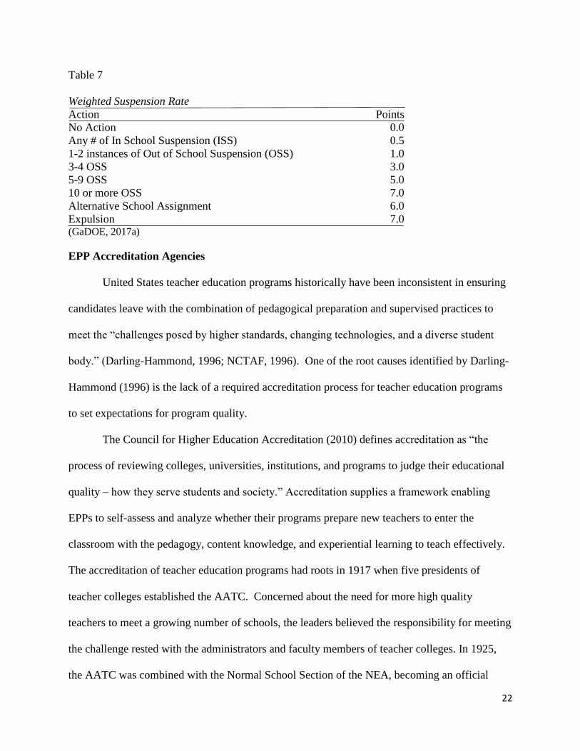
Student suspension data was obtained from the weighted suspension rates located in the
School Climate portion of the 2017 CCRPI. The data is uploaded to GaDOE from the school
district student information systems. Student-level data is then weighted based on Table 7. The
sum of the individual suspension weights is then divided by the total number of enrolled
students.
22
Table 7
Weighted Suspension Rate
Action Points
No Action 0.0
Any # of In School Suspension (ISS) 0.5
1-2 instances of Out of School Suspension (OSS) 1.0
3-4 OSS 3.0
5-9 OSS 5.0
10 or more OSS 7.0
Alternative School Assignment 6.0
Expulsion 7.0 (GaDOE, 2017a)
EPP Accreditation Agencies
United States teacher education programs historically have been inconsistent in ensuring
candidates leave with the combination of pedagogical preparation and supervised practices to
meet the “challenges posed by higher standards, changing technologies, and a diverse student
body.” (Darling-Hammond, 1996; NCTAF, 1996). One of the root causes identified by Darling-
Hammond (1996) is the lack of a required accreditation process for teacher education programs
to set expectations for program quality.
The Council for Higher Education Accreditation (2010) defines accreditation as “the
process of reviewing colleges, universities, institutions, and programs to judge their educational
quality – how they serve students and society.” Accreditation supplies a framework enabling
EPPs to self-assess and analyze whether their programs prepare new teachers to enter the
classroom with the pedagogy, content knowledge, and experiential learning to teach effectively.
The accreditation of teacher education programs had roots in 1917 when five presidents of
teacher colleges established the AATC. Concerned about the need for more high quality
teachers to meet a growing number of schools, the leaders believed the responsibility for meeting
the challenge rested with the administrators and faculty members of teacher colleges. In 1925,
the AATC was combined with the Normal School Section of the NEA, becoming an official

23
department with complete autonomy (Ducharme & Ducharme, 1998). The organizational
constitution and bylaws established a committee on accrediting and classification. In 1947, the
AATC merged with the National Association of Colleges Departments of Education and the
National Association of Teacher Education Institutions in Metropolitan Districts to form the
AACTE. One of the charges for the newly created organization, as articulated by Charles Hunt,
a pivotal leader in AATC and AACTE, was to strengthen the work of the Accrediting Committee
(Popham, 2015).
AACTE published Revised Standards and Policies for Accrediting Colleges for Teacher
Education in 1950, the first of several standards for accreditation. After years of balancing the
desire to serve as both a professional association for diverse institutions, ranging from small
teacher colleges to schools of education situated within large institutions, and an accrediting
body, the NCATE was created in 1954. The goals of the NCATE were to “establish rigorous
standards for teacher education programs” and hold accredited institutions accountable for
maintaining articulated standards. Additionally, NCATE hoped to encourage unaccredited
schools to utilize the NCATE’s standards to ensure program quality (NCATE, 2014). NCATE
required schools of education seeking education to complete a conceptual framework, or “shared
vision of the unit’s efforts in preparing educators to work in P-12 schools,” in addition to
addressing their efforts to meet that six overarching NCATE unit standards and the standards
associated with the corresponding specialized professional association, or NCATE subgroup. In
the 1980’s, Arkansas, North Carolina, and West Virginia required NCATE accreditation for all
schools of education (NCATE, 2014). Table 8 lists the NCATE’s six unit standards. (Popham,
2015).

24
Table 8
NCATE Unit Standards
Standard Standard Name Number of
Number Critical Elements
1 Candidate Knowledge, Skills, & Professional Disposition 7
2 Assessment System and Unit Evaluation 3
3 Field Experience and Clinical Practice 3
4 Diversity 4
5 Faculty Qualifications, Performance, and Development 6
6 Unit Governance and Resources 5
The CSSO established the INTASC in 1987 to foster collaboration among states
interested in enhancing extant teacher preparation, induction, and initial licensing standards. In
1992, INTASC published Model Standards for Beginning Teacher Licensing, Assessment, and
Development: A Resource for State Dialogue. The Standards were developed by practitioners
and representatives from seventeen state agencies to move the needle on the discussion of “the
knowledge, dispositions, and performances” that demonstrate teacher quality for all teachers,
regardless of content area and grade level (CSSO, 1992). They formed a template for what
beginning teachers should continuously practice and reflect upon in order to improve their
effectiveness and prepare them for National Board Certification, the most respected professional
certification granted to exemplary veteran teachers. Additionally, INTASC sought to encourage
all state agencies to rethink current training and licensing standards and identify opportunities for
continuous improvement. Renamed InTASC, to reflect the organization’s commitment to
supporting teachers throughout the development continuum, the Standards were updated in 2011
to reflect a move towards documenting how practice standards are demonstrated at varying
career developmental stages as well as aligning the Standards with recently published national
and state standards documents.

25
In 1997, TEAC was created as an alternative of NCATE, criticized by some for having
minimal standards and a time-consuming accreditation process (Popham, 2015). TEAC’s
overriding goal is to advance P-12 student learning by supporting the preparation of competent,
caring, and qualified professional educators through recognizing, assuring, and promoting high
quality teacher education programs (TEAC, 2013).
In 2009, organizations such as the AACTE, CSSO, NCATE, and TEAC advocated to
develop a “model unified accrediting system” that not only combined the strengths of NCATE
and TEAC but raised the stature of the teaching profession through heightened quality assurance
of teacher preparation programs (Brittingham et al., 2010). In 2010, NCATE’s Blue Ribbon
Panel on Clinical Preparation and Partnerships for Improved Student Learning published their
recommendations on principles and strategies for creating programs “grounded in clinical
practice and interwoven with academic content and professional courses (NCATE and TEAC,
2010).”
NCATE and TEAC merged in 2013 to create CAEP. CAEP’s mission was to “advance
equity and excellence in educator preparation through evidence-based accreditation that assures
quality and supports continuous improvement to strengthen P-12 student learning” (CAEP,
2015b). The five CAEP standards are derived from the beliefs that quality educator preparation
programs produce competent, caring graduates and are comprised of faculty who create “a
culture of evidence” and utilize it to ensure the quality of program offerings (CAEP, 2015a).
Georgia Professional Standards Commission
The GaPSC is one of twelve independent state standards boards that regulate licensure,
teacher preparation program standards and approval, and professional conduct (National
Association of State Directors of Teacher Education and Certification, 2010). Created by the

26
Georgia General Assembly in 1991, GaPSC aims “to build the best prepared, best qualified and
most ethical educator workforce in the nation.” (GaPSC, 2015). The GaPSC is responsible for
the preparation, certification, and professional conduct for public school-based certified
personnel, such as administrators, teachers, and paraprofessionals. Georgia has a tiered teacher
certification system, which fosters teacher growth by recognizing the professional learning needs
and contributions of teachers at different career stages. The certification tiers are as follows:
• Pre-service;
• Induction;
• Professional;
• Advanced Professional;
• Lead Professional. (GaPSC, 2016b).
Pre-Service candidates are those admitted to state-approved educator preparation
programs. Certificate holders are cleared to participate in program activities culminating in
supervised field experience, clinical practice, student teaching, or residency work. The GaPSC
sets the following requirements for the attainment of the Pre-Service certificate:
• admittance to state-approved educator programs that lead to the Induction teaching
certificate and requires participation in field experiences or clinical practice in
Georgia schools;
• Pre-Service certification (must be requested by an EPP);
• background check;
• completion of the Georgia Educator Ethics – Program Entry Assessment (GaPSC,
2016c).

27
Pre-service candidate holders have five years to complete the educator program. GaPSC defines
clinical practice as residency or internship that provides teacher candidates with a culminating
activity that immerses them in the learning community and provides opportunities to develop and
demonstrate competence (GaPSC, 2017b).
The Induction Certificate, granted to teachers with fewer than three years of experience,
facilitates the professional growth for early career teachers. There are three pathways that vary
based on where the educator completed their educator program and/or student teaching. Those
pathways have the following requirements:
• completion of a state-approved educator preparation program;
• passing score on the appropriate GACE (or comparable) content assessment;
• passing score on the Georgia Educator Ethics Assessment – Program Exit;
• course in identifying and educating exceptional children (Pathway 3 candidates do
not have to complete the course prior to being granted the Induction certificate but
must complete it before being reissued an Induction certificate or conversion to a
Professional certificate.);
• passing score on state content pedagogy assessment. Georgia’s assessment is the
edTPA. (Pathway 3 candidates do not have to complete the assessment prior to being
granted the Induction certificate but must complete it before being reissued an
Induction certificate or conversion to a Professional certificate).
The fourth pathway addresses teachers hired prior to completing an educator preparation
program. Pathway teachers must complete a state-approved educator preparation program and
pass the edTPA for conversion to another Induction pathway or Professional Certificate.
Requirements for the Induction Certificate include:

28
• Bachelor’s degree or higher;
• passing score on the GACE Program Admission Assessment, or exemption;
• passing score on the appropriate GACE (or comparable) content assessment;
• passing score on the Georgia Educator Ethics Assessment – Program Entry (GaPSC,
2016c).
The Professional certification is granted to educators with at least three years of
experience within the last five years. There are two types of certificates, performance and
standard, which vary based on whether the teacher completed a Georgia performance-based
certification program and has been evaluated for at least two years via Georgia’s TKES. In
addition to current employment and the length of teaching experience, teachers requesting either
certificate must have a professional level passing score on the appropriate GACE content
assessment. Performance-based certificate holders must have earned at least two Proficient or
Exemplary annual TKES performance ratings. (GaPSC, 2017b).
GaPSC defines state-approved programs as professional education programs, provided by
colleges/universities, school districts/systems, RESAs, or private providers based on established
state standards and delivered as traditional or alternative certification routes (GaPSC, 2016d).
Regionally accredited institutions, LEAs over 30,000 students, RESAs, and other education
service agencies are eligible to apply to become an EPP. GaPSC approval standards are adapted
from the CAEP Standards; in fact, CAEP approval is considered a route to EPP approval.
Programs receiving initial (Developmental) approval have three years to demonstrate that they
have the capacity to meet GaPSC standards prior to the First Continuing Review. Unless
performance data or a previous review indicates standards not being met or the existence of
pervasive problems or non-compliance with GaPSC rules, Continuing Reviews of EPPs are

29
conducted every seven years. Appendix B contains a list of the EPPs approved for initial
certification programs (GaPSC, 2018b).
With some documented exceptions, GaPSC requires the following admission
requirements for initial certification programs:
• possess a 2.5 grade point average (post-baccalaureate program applicants must have a
2.5 G.P.A. in major or applicable content area in the certification field);
• pass the Program Admission Assessment;
• pass the Assessment of Educator Ethics – Program Entry;
• pass a criminal background check;
• be eligible to receive a Pre-Service Certificate (GaPSC, 2018a).
GaPSC (2018a) has the following program content and curriculum requirements:
• incorporate the InTASC Model Core Teaching Standards;
• 15 (Middle Grades) or 21 (Secondary) semester hours of content field coursework
• coursework regarding professional ethics, ethical decision-making, and the Georgia
Code of Ethics for Educators;
• coursework ensuring candidates are prepared to implement the applicable state-
approved content standard by developing and delivering lesson plans which
emphasize “critical thinking, problem solving, communication skills, and peer
collaboration.”
• familiarity with the state teacher evaluation system;
• technology proficiency;
• coursework addressing the nature and needs of Special Education students and
differentiated instruction;

30
• coursework regarding methods for teaching reading for Early Childhood Education
candidates.
The state of Georgia requires all teacher preparation program providers to annually report
on TPPEM. Outcome and program measures are weighed equally and are designed to capture
teacher candidate performance while enrolled in the program and their performance after
program completion. Outcome measures include:
• employers’ perceptions of preparation (20% of Outcome Measure), as measured by a
state-wide survey;
• teacher observation data (30%), as measured by the summative ratings for the
Teacher Assessment on Performance Standards (TAPS) instrument, Georgia’s teacher
evaluation tool. (GaPSC, 2017c)
Program measures include:
• Assessment of Teaching Skills (30%), utilizing edTPA;
• Assessment of Content Knowledge through the GACE content assessment (10%);
• Completers’ Perceptions of Preparation (10%) as measured through an annual state-
wide survey (GaPSC, 2017c).
Beginning in the 2018-19 school year, EPPs and their offered programs will be annually
identified at the following performance levels based on TPPEM: exemplary, effective, at-risk of
low performing, or low performing. Programs at the at-risk of low performing or low
performing levels receive additional approval reviews or monitoring. Failure to improve their
performance level over three years results in a recommendation to the GaPSC for revocation of
program approval. GaPSC requires EPPs to form partnerships with schools and LEAs to
facilitate field experiences and clinical practice. GaPSC (2018a) defines field experiences as

31
activities that include organized, sequenced, and substantive engagement of candidates providing
opportunity to observe, practice, and demonstrate standards-based knowledge and skills.
Candidates are required to participate in at least two different grade levels consistent with the
certification being sought. The candidates should be provided regular opportunities to apply,
reflect upon, and expand their capacity for teaching and learning.
Clinical practice, also referred to as internships or residency, immerses teacher candidates
in a learning community where they can more intensely practice and apply their growing
knowledge, skills, and dispositions. Clinical practice must last for at least one semester. Teacher
candidates participating in clinical practice, regardless of the duration, are supervised by a
veteran (at least three years of experience) teacher who is certified in the same content area and
has agreed to provide ongoing support throughout the experience (GaPSC, 2018a). The GaPSC
(2018a) recognized in Rule 505-3-.01 the added value of a year-long residency where teacher
candidates fully participate at a school as a member of the faculty for the entire school year,
including participation in site-based induction programs, parent-teacher conferences, teacher
meetings, and professional learning opportunities.
Teacher Preparation
What Matters Most: Teaching or America’s Future (NCTAF, 1996) establishes the
importance of recruiting, preparing, and retaining good teachers as the central strategy for school
improvement and that school reform must focus on creating the conditions for teachers to be able
to teach well (NCTAF, 1996). Research has shown that teacher effectiveness depends on the
breadth and depth of one’s content knowledge and pedagogy. As a result, increased focus has
been placed on the notion that improving teaching will result in increased student achievement.

32
Teaching existed long before teacher education (Labaree, 2008). For the first two
hundred years of public education in America, teacher certification was left up to LEAs (Roth &
Swail, 2000). Teachers had to demonstrate sound moral character, complete the eighth grade,
and, in some districts, pass a basic knowledge test. By 1867, most states required aspiring
teachers to pass a basic skills test which also assessed knowledge of United States history,
geography, spelling, and grammar (Ravitch, 2003).
The nineteenth century saw the development of normal schools, two-year programs
offering educational methods courses for elementary school teachers. The Common School
movement, led by Horace Mann, held as a core tenant the belief that education was key to
citizenship, democratic participation, and social harmony. As a result, the idea of universal
schooling was to provide every child with taxpayer-funded basic education, with an emphasis on
literacy on citizenship. Normal schools aimed to ensure teacher quality for these common
schools by providing norms for pedagogy and curriculum through a “thorough, cohesive, and
scientific curriculum” (Public Broadcasting System, 2018). Early in the formation, normal
schools prioritized developing academic content knowledge, due to the vast differences in
knowledge of prospective teachers combined with their need to teach diverse student ability
levels in the same classroom. By 1900, sixty years after the founding of the first normal school,
there were 330 normal schools training 115,000 prospective teachers (Levine, 2011). As more
graduates and practitioners became normal school faculty, around the turn of the twentieth
century, the coursework focus shifted toward the child development, pedagogy, classroom
management, and the development of social and citizenship skills (Alkhudhair & Ball, 2012). In
addition to Normal Schools, some states, such as New York, subsidized private academies for

33
teacher preparation, while some LEAs in urban and rural areas developed their own teacher-led
teacher preparation programs.
Around the turn of the century, the growth of high schools and the birth of professional
organizations and accreditation programs led to major changes in teacher preparation. Colleges
and universities created teacher education programs initially to train secondary school teachers
on-site in order to increase access to subject matter coursework. As pressure to further
professionalize teaching mounted, many public normal schools became state teacher colleges,
expanding to four-year programs, increasing admission and graduation requirements while
enhancing their liberal arts content teaching and adding arts and science content emphasis. By
the mid-twentieth century, the notion of a state teacher college was nearly obsolete, as post-
World War college enrollment increases prompted degree program expansions at these
institutions. State Teacher Colleges became colleges of education found within a larger
institution.
The overall organization of EPP curriculum has its roots in the teacher preparation model
advocated by Teachers College Dean James Earl Russell in the early twentieth century. The
model included:
• general culture: culture that inspires respect for knowledge and the pursuit of truth.
Additionally, preparation that fostered interrelationships among the different fields of
knowledge.
• special scholarship: command of subject knowledge and the development of
reflective inquiry that enables teachers to be adaptive to the need of students;
• professional knowledge: understanding of how one’s subject connects to other subject
areas and the world;

34
• technical skill: pedagogical knowledge that enables one to know what to teach, the
sequence in which it should be taught, what methods, and to whom (Cremin, 1978).
By the 1950s, it was common for aspiring teachers to receive preservice education through a
university or college (National Academy of Sciences, 2010). During the 1970s, recruitment
incentives, such as scholarship programs for future teachers, Urban Teacher Corps initiatives,
and the introduction of Master of Teacher programs, combined with wage increases, dramatically
increased the supply of new teachers. However, the cancellation of many of these programs in
the 1980s and 1990s resulted in new shortages as student enrollment in public education rose.
That time period also witnessed the birth of additional alternative teacher programs, in which
new teachers received probationary certification upon hire and were given up to five years to
complete a certification program while teaching full-time.
Approximately 460,000 individuals were enrolled in teacher preparation programs during
the 2013-2014 school year (USDOE, IES, 2016b). In 2009, there were approximately 1,450
schools, colleges, and departments of education located at 78% of four-year colleges and
universities (Duncan, 2010). More than 200,000 students complete an educator preparation
program each year from over one thousand four-year bachelor’s degree and one-year post-
baccalaureate programs housed in colleges and universities (National Academy of Sciences,
2010). Colleges of education annually award 8% of all bachelor’s degrees, 25% of all master’s
degrees, and 15% of doctorates. These programs serve as the pathway to the teaching profession
for 70-80% of teachers. There are also 130 alternative education pathways, such as Teach for
America, that provide an additional route to the teaching profession.
While there are numerous pathways to teaching, historically, most have been categorized
as “traditional” or “alternative.” Traditional programs are usually located within colleges and

35
universities and lead to a bachelor’s or master’s degree. Alternative programs are generally
housed by a LEA or private educational organization and are designed to prepare candidates who
lack certain required credentials for the classroom. There is considerable overlap between
traditional and alternative programs as they tend to offer similar coursework and/or field
experiences (Walsh & Jacobs, 2007). The number and lack of distinction of pathways have
resulted in only a handful of students attempting to explore whether traditional or alternative
pathways are more effective. The evidence obtained from the research is mixed (National
Academy of Sciences, 2010). Some of the studies using various research designs suggest
minimal or no difference between the broad pathways (Allen, 2003, Constantine et. Al, 2009;
Wilson, Floden, & Ferrini-Mundy, 2001). Other studies identified small differences (Glazerman,
Mayer, and Decker, 2006; Xu, Hannaway, and Taylor, 2008). The mixed findings indicate that
there are opportunities for exploration of program effectiveness; however, the broad categories
fail to capture programmatic differences that may add to the body of evidence of what
characteristics significantly impact program quality, thus leading to teacher quality, retention,
and student achievement.
There is a body of research that the foundation of an effective EPP is a strong, shared
vision of teaching and learning and coherent, consistent goals and standards that are interwoven
in coursework and clinical practice (Darling-Hammond & Bransford, 2005; Howey & Zimpher,
1989; Levine, 2006; Merseth, K. & Koppich, 2000). In Table 9, Principals, Education Program
Alumni, Faculty, and Deans were asked to select the three most important proposals to
improving teacher education. The top response for Principals and Alumni, and the second for
faculty, was for more coherence between coursework and field experiences. One-third of

36
surveyed Principals, and around a quarter of Education Program alumni, faculty and deans view
extending the duration of student teacher as critical to improving teacher preparation.
Clinical education provides pre-service teachers with practical and skill-oriented
instruction under the supervision of an experienced teacher (Florida Department of Education,
2018).
Table 9
Most important proposals for improving teacher preparation programs
Percent
Proposal Principals Alumni Faculty Deans
Better balance between subject matter 57 69 49 13
preparation and field experience
Require longer student teaching 31 26 22 23
experience
Provide closer supervision of student 18 21 21 21
teaching
Divide professors into clinical and 6 14 16 13
research categories
Mentor new teachers 50 63 69 70
Require a major in an academic 17 27 34 24
subject
Increase mastery of pedagogical 26 27 41 43
practice
Raise requirements for academic 7 14 23 17
performance
Recruit higher quality faculty 7 16 13 8
(Levine, 2006)
Most teacher preparation programs include student teaching as the capstone experience for
teacher candidates. However, the length or content of student teaching, is not equal across
programs or states. For instance, the student teaching capstone experience is typically at most a

37
semester where candidates have opportunities to teach and learn alongside an experienced
practitioner at a local school or community center. Other programs blend coursework and
experiential learning, with candidates spending several hours a week in university courses
learning pedagogy and several more observing or working in classrooms. State requirements for
capstone experiences range from thirty hours to three hundred hours. According to Levine
(2006), 60% of teachers reported a semester-long student teaching experience, with 20% having
a longer one, and 20% having less than a semester.
Clinical experiences should enable pre-service teachers to reinforce, apply, and
synthesize concept, ideas, and theories addressed in their coursework. Learning is enriched when
candidates have multiple, diverse opportunities to see the connections between theory and
practice. Levine (2006) interviewed recent education program graduates about the number of
field experience placements. Only 8% of respondents were placed in three or more different
classroom settings, with 38% placed in two. Extreme care should be taken to ensure candidates
are provided meaningful and frequent mentoring opportunities with EPP and school-based
faculty (Darling-Hammond and Bransford, 2005; Levine, 2006).
Concerns and Proposed Solutions Regarding EPP Quality
There has generally been a great deal of disagreement regarding the character, content,
and caliber of education and preparation prospective teachers should have to be qualified to teach
(Ingersoll, Merrill, & May, 2014). Historically, teacher preparation programs have been
criticized for not having a sufficiently selected admission process, resulting in students with
weaker academic credentials than their non-teacher education program counterparts (Hess,
Rotherham, & Walsh, 2004). However, the lack of reliable data showing the relationships
between pre-service teacher preparation, teacher quality, and student learning, has complicated

38
the debate on the most effective teacher preparation models and has, in some part, led to the
growth of policies supporting alternative routes to teacher certification (Glazerman, Mayer, &
Decker, 2006; Walsh 2001; Walsh & Jacobs, 2007).
Crowe (2010) notes that the current state oversight of teacher education programs does
not guarantee program quality or hold programs to high enough standards to meet student needs.
Quality control is further complicated by the fact that there is no uniform method for program
oversight; every state provides its own standards and guidelines. One of the critiques of state
standards is that the program requirements assure a base level of uniformity, but do not provide
substantive quality guidelines. For instance, while GaPSC does set parameters on the minimum
length of student teaching and the teaching experience of the supervising teacher, it is, at best,
vague regarding the quality or mentoring capabilities of the supervising teacher, or school
requirements for supporting preservice teachers.
Concerns have been raised that teacher preparation programs are inadequately preparing
pre-service teachers for today’s standards-based, accountability-driven classrooms. According to
the 2011-2012 Schools and Staffing Survey (USDOE, IES, 2013), 2.5% and 22% of public
school teachers with five years of less teaching experience noted that they were not prepared or
only somewhat prepared, respectively, to meet state content standards in their first year of
teaching. Low admission and graduation standards, variation in quality programs, disconnect
between what is taught by college faculty and what practitioners do in the classroom, and
ineffective state and accreditation standards are factors that may be jeopardizing the relevance of
teacher education programs.
Governmental agencies, accrediting organizations, colleges and universities, education
nonprofits, and teachers’ unions have all proposed ways to redefine EPPs and hold them more

39
accountable for the quality of their graduates (NCATE 2010; USDOE 2011; Greenberg, McKee,
& Walsh, 2013; CSSO, 2012; American Federation of Teachers 2012; NEA 2011). Perhaps an
important aspect of a successful education certification program is ensuring teachers are prepared
to handle the challenges they will face as educators and to provide opportunities for teacher
candidates to determine whether teaching provides the tangible and intangible rewards necessary
for them to make it their career plan. In a 2013 Policy Brief, the NEA proposed that teachers
should be “profession ready” upon serving as a teacher of record, meaning that prior to a
teacher’s first day, EPPs must ensure:
• teacher candidates must be certified in the subject they teach and demonstrate deep
subject matter understanding through a combination of coursework and assessments.
• teacher candidates must demonstrate pedagogical content knowledge in the subject
they teach by being able to anticipate common student mistakes and/or
misunderstandings and to create a positive, engaging classroom environment.
Teachers attain these skills by integrating the theoretical underpinning gained in
“coordinated, coherent coursework” with school-based experiences (NEA, 2013).
• pre-service, classroom-based performance assessments enable candidates to
demonstrate the subject matter and pedagogical understanding while reflecting on
their practice and observations.
Research indicates that teachers do find field experiences useful in their transition into
the teaching profession (Papay, West, & Fullerton, 2012; Ronfeldt, 2012; Urban Teacher
Residency United, 2013). In their study of New York City-area EPPs, Boyd et. al. (2008) found
that programs that provided more classroom-based opportunities and congruence of student
teaching placement produced more effective first year teachers. There is body of research that
40
indicates graduates of residency programs remain in teaching longer than peers from other
certification pathways and feel prepared to handle the subject-matter, instructional planning,
pedagogical knowledge, and classroom management necessary to foster student achievement
(Levine, 2006). However, there is a lack of research-based conclusions about the impact the
length of teacher candidate clinical experiences on teacher retention and student achievement or
on effectiveness of various kinds of clinical experiences. Much of the limited research utilizes
case-study methodologies, making it difficult to determine causality or generalizability (Boyd et.
al. 2008).
The NEA has outlined the following components that must be incorporated in high-
quality clinical experiences:
• partnership between the teacher education program and LEAs to ensure coherence
and consistency between coursework and experiences;
• ongoing opportunities for teacher candidates to teach, analyze, and reflect on their
experiences and learning with clinical supervisors, mentor teacher, and peers;
• ongoing opportunities for observe exemplary and diverse teaching and practices;
• residency experiences grounded in professional standards;
• regular use of data to inform and improve practice (NEA, 2014).
Many school districts are partnering for non-profit organizations and colleges and
universities to establish fellowship or residency programs. These programs usually possess three
core characteristics:
• active partnerships between preparation programs, districts, and stakeholders;
• program selectivity of candidates;

41
• academic coursework coordinated with the development and implementation of
clinical experiences (NEA, 2014).
Programs, such as the Woodruff Fellows and Chicago Teacher Residency generally provide
stipends to recent college graduates and individuals seeking career changes so that they can
spend one year immersed in a combination of student teaching and graduate coursework. The
programs operated under a cohort model, where residents take courses and participate in post-
graduation induction activities together. At the end of the year, generally the candidates have
their certification and/or master’s degree, and a job within their sponsoring school district. In
exchange for their involvement in the program, teachers usually are committed to working in the
sponsoring school district for three years. Most fellowship programs offer coaching and other
induction support beyond the initial fellowship year.
NET-Q and CREST-Ed Programs
After setting a goal to increase synergy between itself and metro-Atlanta school districts
to enable meaningful discourse on teaching and learning, GSU’s College of Education and
Human Development was awarded a five-year, $6.5 million grant in FY2003 by the USDOE for
the creation of PDS2. Professional development school partnerships are specialized partnerships
between universities and schools. Schools benefit from increased, customized professional
development, opportunities to train and hire student teachers, and access to university researchers
and their expertise. The university benefits from its program and faculty members being more
rooted in schools, increased integration and relevance of clinical and academic coursework,
access to subjects and/or data for continued research, and student teachers being more prepared
upon graduation (Levine, 2006). Because of the partnership, there is more interaction between

42
mentor teachers and supervising university faculty, as they craft a program that builds both the
student teacher and classroom student’s competence.
PDS2 enabled GSU faculty to collaborate with metro-Atlanta schools in sharing current
research and strategies to impact teaching and learning, as well as designing professional
development. Building from the success of PDS2, GSU received at $13.5 million Teacher
Quality Partnership Grant in FY2009 to establish the NET-Q project. NET-Q aimed to not only
increase the quality and number of highly qualified teachers committed to Georgia high needs
schools but to ensure new teachers receive the necessary support to thrive and remain in the
classroom. As part of the grant, GSU partnered with six metro-Atlanta school districts, twenty-
three rural Georgia districts, four Georgia colleges, Georgia Public Broadcasting, and the
NCTAF (Miller, 2011).
One component of NET-Q was a post-baccalaureate residency program. Participants
earned initial certification and either a Master of Arts in Teaching (Math and Science residents)
or Master of Education (Special Education residents) during a fourteen-month training period.
The program consisted of rigorous training courses that infused SWD, ELL, and literacy
strategies across content areas and were paired with their classroom work. In addition to
coursework, residents were placed for one year with a qualified mentor teacher in a high-need
area school. Residents were paired with mentor teachers who received training through GSU and
demonstrated effective instructional skills and strategies. Residents received a $25,000 living
stipend so that they could focus on their coursework and residency. Upon the end of the
program, residents were usually hired by their school district and were committed to teaching in
a high-need school in that district for a minimum of three years. GSU’s commitment to the
residents extended beyond graduation in the form of induction programs and professional

43
learning opportunities (GSU, 2018a). Through NET-Q, GSU saw a 12% increase in STEM
teacher production the number of male candidates from traditionally underrepresented groups.
Additionally, 92% of program graduates remained in teaching past their third year (Ross, 2014).
In FY2014, the USDOE awarded GSU $7.5 for its CREST-Ed program. CREST-Ed
partners with Albany State University, Columbus State University, the National Commission on
Teaching and America’s Future, and nine school districts to recruit, train, and support 250-300
future STEM teachers (GSU, 2018b). CREST-Ed aims to increase the number of highly qualified
teachers working in rural or urban settings through the following initiatives:
• enhancing undergraduate teacher preparation programs through extended field
experiences, co-teaching and STEM activities;
• enhancing graduate teacher preparation programs through residencies that include
strong mentor training;
• promoting STEM through professional development, faculty liaisons and access to
advance credentialing support (GSU, 2018b).
As with NET-Q, pre-service teachers will participate in year-long teacher residencies at partner
schools and receive a living stipend. In the fall, students work in their schools for four days and
come to GSU for a “CREST-Ed work session” one day. In the spring semester, students work
full-time at their partner schools. School placement is determined through interview with the pre-
service teacher, partnering school, and CREST-Ed faculty. In addition to certification and
graduate program work, residents conduct a classroom-based research project that is presented
during a poster session at the CREST-Ed Summer Institute, a conference for residents, partnering
schools, GSU faculty, and prospective teachers. Following the eighteen-month program,
CREST-Ed alumni continue to be supported through their first two years of teaching through

44
cohort resource sharing, monthly communication with CREST-Ed faculty, and classroom visit,
as requested (GSU, 2018c).
Another unique feature of the Crest-Ed program is the use of TIP-AAR. Using TIP-
AAR, instructional units are developed collaboratively with a classroom teacher, intern, and
university professor, based on the content deficiencies observed after looking at student
formative and summative assessment data. Both the teacher and intern administer a common
pre-test, implement the units utilizing various data-driven instructional supports and
interventions, and administer a common post-test in their respective classrooms. A mixed-
methods AAR approach is then utilized to measure student achievement and growth from both
an inter- and intra-classroom perspective. In their meta-analysis of ten TIP-AAR studies,
Curlette, Hendrick, Ogletree, and Benson (2014) found student achievement gains in the intern-
taught classrooms exceeded the gains in the comparison teacher classrooms.
Propensity Score Analysis
PSA includes several statistical methods utilized in observational studies or quasi-
experiments, where causal modeling is sought when randomized assignment of interventions is
either infeasible or unethical. Described by Guo and Fraser (2015) as a fusion of econometric
tradition that focuses on structural equation modeling in studying causality and a statistical
approach that relies on randomized fusion, PSA offers an approach to program evaluation for
researchers needing to estimate treatment effects and control for covariates with observational
data. Rubin (1974) argued that in the social sciences, conducting randomized experiments is
problematic due to observational data being the only available data, prohibitive costs for
conducting randomized experiments, ethical reasons preventing random assignment, and the time
(years) that may be required to carry out and receive results for an experiment. When

45
randomized clinical trials are not feasible, PSA aids in removing selection bias in quasi-
experimental designs. Additionally, conducting an ordinary least square regression using a
dichotomous indicator of treatment leads to inflated and biased treatment effect estimates, due to
the error term being correlated with explanatory variables. PSA enables analysis of causal effects
in observational studies.
PSA has been utilized in a variety of disciplines and professions, including education
(Morgan, 2001), economics (Heckman, Ichimura, & Todd, 1997; LaLonde, 1986;
Michalopoulos, Bloom, & Hill, 2004), epidemiology (Normand et al., 2001), psychology (Jones,
D’Agostino, Gondolf, & Heckert, 2004), social work (Barth, Gibbons, & Guo, 2006; Barth, Lee,
Widlfire, & Guo, 2007; Weigensberg, Barth, & Guo, 2009), and sociology (Smith, 1997). The
approach is based on the potential outcomes framework conceptualized by Neyman (1923).
Neyman’s work focused on randomized experiments; it wasn’t until the late 1970s and 1980s
when the framework was initially applied to observational studies (Heckman, 1978; Heckman,
1979; Rosenbaum & Rubin, 1983). The model, also known as the Neyman-Rubin counterfactual
framework of causality, holds that individuals assigned to treatment or non-treatment groups
have potential outcomes in both states. A causal relationship cannot be inferred without
comparing the outcomes under both the treated and untreated conditions. The relationship can
be expressed as the following:
𝑌𝑖 = 𝑊𝑖𝑌1𝑖 + (1 − 𝑊𝑖)𝑌0𝑖,
where 𝑌𝑖 = outcome variable, 𝑊𝑖 = receipt of treatment, 𝑊0 = receipt of non-treatment, 𝑌1𝑖 =
potential outcome of treatment, and 𝑌0𝑖 = potential outcome of non-treatment (Guo and Fraser,
2015).To resolve what Holland (1986) describes as the fundamental problem of casual inference,
the Neyman-Rubin counterfactual framework of causality holds that the counterfactual can be

46
assessed by evaluating the difference in mean outcomes between the two groups. The treatment
effect is defined as:
𝜏 = 𝐸(𝑌1|𝑊 = 1) − 𝐸(𝑌0|𝑊 = 0).
As a result, the above equation can be viewed as an attempt to estimate the mean outcomes of the
untreated if they had been exposed to the intervention (Guo and Fraser, 2015).
Counterfactual models are dependent on two assumptions: ignorable treatment
assignment assumption and stable unit treatment value assumption. The ignorable treatment
assignment assumption holds that the treatment assignment is independent of the potential
outcomes after controlling for covariates, expressed as
(𝑌0𝑌1) ⊥ 𝑊|𝑋,
where Y0=outcome of non-treatment, Y1=outcome of treatment, W=assignment of study
participants to treatment, X = covariates (Guo & Fraser, 2015). Violation of the ignorable
treatment assignments assumption can lead to biased and inconsistent estimation of the treatment
effect. SUTVA maintains that the potential outcomes for a unit do not interfere with the
treatments assigned to another, and there is a single version of each treatment level (Imbens &
Rubin, 2015). Several models have been developed to either correct for biases under the
condition of nonignorable assignment or relax the assumption by doing one of the following:
• employing approaches not reliant on strong assumptions requiring distributional and
functional forms;
• rebalancing assigned conditions to better replicate randomized-generated data;
• estimating counterfactuals through various statistical techniques (Guo and Fraser,
2015).

47
Chi-square tests or other analysis can be conducted between the treatment variable and each
independent variable to test the tenability of the ignorable treatment assignment assumption.
A propensity score is a conditional probability that a unit with certain explanatory
variables will be assigned to a treatment instead of a control group. Participants are placed into
comparable groups, or strata, at the beginning of the study. By balancing covariates between the
groups, researchers can approximate a random experiment, reducing or eliminating selection bias
in observational data analysis (Cochran & Chambers, 1965).
In a randomized experiment, the randomization of units to different interventions
generally ensures no systematic covariate differences between units assigned to the different
treatments. In observational studies, direct outcome comparisons between treatment groups
cannot be made due to the treatment assignment not being randomized. This limitation can be
overcome if information on measured covariates is either incorporated into the study design or
treatment effect estimation. According to D’Agostino (1998), traditional methods of adjustment,
such as matching, stratification, and covariance adjustment, are often limited since they can only
use a limited number of covariates for adjustment. Since propensity scores are a scalar summary
of the covariate information, they may be better suited for comparisons.
The properties of propensity scores are as follows:
• propensity scores balance differences observed in each covariate between treated and
control groups. Any differences between groups are random rather than systematic
differences.
• treated and control participants with similar propensity scores have the same
distribution of X.

48
• conditional on the propensity score, treatment assignment and observed covariates are
independent of each other.
• the expected differences in responses between groups at 𝑒(𝑥𝑖) is equal to the ATT at
𝑒(𝑥𝑖).
• the expected differences in responses between matched units with the same
propensity score equals the ATT at 𝑒(𝑥𝑖) (Rosenbaum & Rubin, 1983).
PSA generally begins with determining the observed covariates affecting selection bias and
obtaining an optimal estimate of propensity scores, usually by constructing models using logistic
regression, probit regression, discriminant analysis, or Mahalanobis metric distance. There are
five main analyses that can be conducted once propensity scores are estimated:
• matching or resampling participants, or PSM;
• Propensity score subclassification: multivariate analysis where the sample is
subclassed such that participants within a stratum are homogeneous on identified
covariates. The ATE is the average of the estimated treatment effects in each stratum.
• Propensity score weighting: multivariate analysis using propensity scores as sampling
weights separately for treated and control participants, as well as for ATE and ATT;
• Matching estimators: a vector norm is used to directly impute potential outcomes
(counterfactuals) for the study participants. Matching estimators can then be used to
estimate various ATTs.
• PSA with nonparametric regression model: nonparametric regression is used to
generate propensity scores derived from multiple matches. The propensity scores are
then used to compute the counterfactual, in the form of a weighted mean.

49
PSA can also be utilized for models with multiple treatments, continuous treatment doses, and
time-varying treatments (Leite, 2017). Based on the model used, post-model analysis is
conducted to measure the ATT and its statistical significance.
Propensity Score Matching
PSM is increasingly utilized to minimize selection bias when comparing nonequivalent
groups (D'Agostino, 1998; Fraser, 2004; Guo et al., 2006; Joffee & Rosenbaum, 1999;
Rosenbaum & Rubin, 1983; Rubin, 1997; Sosin, 2002). Propensity score matching address
biased estimates about the treatment effect that can occur when the explanatory variable is
correlated with the error term. Rosenbaum and Rubin (1983) defined the propensity score as the
following:
𝑒(𝑥𝑖) = 𝑝𝑟(𝑊𝑖 = 1|𝑋𝑖 = 𝑥𝑖),
where 𝑒(𝑥𝑖) = propensity score, i = participant (i = 1, …, N), 𝑊𝑖 = 1 is assignment to a
treatment, 𝑊𝑖 = 0 is assignment to nontreatment, 𝑥𝑖 = vector of observed covariates.
By creating a vector, propensity score matching reduces the dimensionality represented
by multiple covariates to a one-dimensional score. This approach results in increased ability to
match control and treatment group participants than with conventional matching approaches,
where losses in study participants can occur as the number of explanatory variables increase.
Additionally, propensity score matching also allows for smaller outcome models with fewer
estimated parameters, because only covariates of theoretical interest are included in the model
(Leite, 2017). As with other counterfactual models, propensity score matching makes
comparisons between the potential outcomes of two hypothetical exposure situations that could
occur.

50
Propensity score matching has been used in various educational research studies.
Morgan, Frisco, Farkas, and Hibel (2008) found that special education services in the early
grades had a positive effect on learning behaviors. Lindekugel (2015) found no statistically
significant improvement in standardized testing based on student participation in high school
band programs. Propensity score matching and regression has been used to evaluate the effects
of local, state, and federal program initiatives on student performance outcomes (Gross, Booker,
and Goldhaber, 2009; Rodriguez, Hughes, & Belfield, 2012; Wyse, Keesler, & Schneider, 2008).
Glazerman and Seifullah (2010) used propensity score matching with a fixed caliper to research
the effects of value-added incentives, as well as structured supports, on teacher retention and
student achievement. The report found no significant evidence that the program significantly
impacted student achievement growth or teacher retention rates after two years of
implementation. Using propensity score matching, Kee (2012) found first year teachers with less
course work and shorter field experiences felt less prepared entering the profession than peers
with more extensive training. Afolabi (2012) utilized one-to-one propensity score matching with
a caliper to measure the relationship of participation in professional learning communities and
teacher retention. The research found new public school teachers participating in professional
learning communities had significant higher retention rates than non-participating peers.
Leite (2017) identifies a six-step procedure for conducting PSM:
• Identify covariates most likely to be causing an imbalance between the treated and
control groups, usually through logistic regression;
• obtain an optimal balance of propensity scores for treated and control groups;
• use the propensity scores to match treated and control participants with similar
propensity scores with greedy or optimal matching algorithms;

51
• evaluate the balance of covariate distributions between treated and untreated;
• estimate the treatment effect and standard error;
• perform post-matching analysis, including sensitivity analysis, multivariate analysis
and regression adjustment.
The most common implementation of propensity score matching is one-to-one (or pair)
matching, in which pairs of treated and untreated subjects are formed, such that matched subjects
have similar values of the propensity score (Austin, 2011). Ratio matching differs from pair
matching as it allows for multiple control matching for each treated individual. While the
sample size increases obtained via ratio matching result in decreased variance of the mean
differences, there may be increased bias as the added control matches are further away from the
first match (Rubin & Thomas, 1996). Variable ratio addresses this limitation by allowing the
ratio of treated to untreated matches to vary. In full matching, matched sets consist of either a
treated unit with at least one control or a control unit with one or more treated units (Gu &
Rosenbaum, 1993).
Greedy matching is a family of algorithms including nearest neighbor, caliper, and
Mahalanobis metric distance, and Mahalanobis metric matching within a caliper. Greedy
matching is a linear matching algorithm that produces matched pairs with balanced covariates
sampled. Using Mahalanobis metric matching, distances are calculated between randomly
ordered treatment participants and controls, using the Mahalanobis distance formula:
𝑑(𝑖, 𝑗) = (𝑢 − 𝑣)𝑇𝐶−1(𝑢 − 𝑣)
where i = treated participant, j = control participant, u and v = values of the matching variables,
and C = sample covariance matrix of the matching variables (Guo & Frasier, 2015). The j value

52
with the minimum distances is chosen as a match for i, and both participants are then removed
from future consideration. The process continues until all matches have been found.
In caliper matching, j is selected as a match to i if the following condition is met:
‖𝑃𝑖 − 𝑃𝑗‖ < 휀, 𝑗 ∈ 𝐼0
where P = propensity scores for treated (i) and control (j) participants and 휀 = caliper size (Guo
& Fraser, 2015). Rosenbaum and Rubin (1985) recommend a caliper size of a quarter of a
standard deviation of the sample estimated propensity scores. For nearest neighbor matching,
control and treated participants are matching if the absolute difference of their propensity scores
is the smallest among all possible pairs of scores. Once a control participant is matched, the
participant is removed from the pool without replacement. Nearest available Mahalanobis metric
matching within calipers defined by the propensity score combines the previously discussed
greedy matching methods, maximizing the balance between the covariates and the covariates’
squares and cross-products between the two groups (Guo & Fraser, 2015; Rosenbaum & Rubin,
1985). After the treated participants are ordered, the control participants within a predetermined
caliper are selected. The control participant with the shortest Mahalanobis distance from i is
chosen. The process is repeated with the next treated participant. According to Leite (2017),
greedy matching works well when the ratio of treated to untreated cases is small. The use of
calipers, setting an allowable maximum distance between matches, provides an evaluation of the
area of the propensity score distribution where treated and control values exist, minimizing
standard errors of the treatment effect and maximizing power. Matching with replacement
enables continued matching of treated cases with the nearest untreated case, regardless of order,
generally reducing bias than when matching without replacement is used, especially when the
number of available matches is small (Rosenbaum, 1989). Greedy matching provides flexibility

53
in evaluating casual effects using a variety of multivariate analyses. Limitations of greedy
matching include the loss of matching when the treated and nontreated cases have extreme
propensity scores in opposite directions.
Alternative models, such as optimal matching, were developed to address the fact that
prior matching decisions are not reevaluated in subsequent iterations. Specifically, the order in
which the treated subjects are matched using greedy matching methods may change the quality
of the matches. Rosenbaum (2002) used set‐theoretic terminology to define a stratification of a
sample:
Let A denote the set of all treated subjects and B denote the set of all control
subjects in the full sample. Then (A1,…, AS, B1,…, BS) denotes a stratification of
the original sample that consists of S strata if the following conditions are met:
• |Ai| ≥ 1 and |Bi| ≥ 1 for i = 1,…,S.
• As∩At=∅ and Bs∩Bt=∅ for s ≠ t.
• A1∪⋯∪AS⊆A and B1∪⋯∪BS⊆B.
The matching process produces S matched sets, each containing |A1| and |B1 | . . . |As| and |Bs|.
A key characteristic of optimal matching is the ability for matches among participants to change
if a different matching will further minimize the total propensity score distance. Optimal
matching can be classified into three types:
• pair matching, where each treated participant is matched to a single control
participant;
• variable matching, where each treated participant is matched to up to four controls;
• full matching, where both classifications of participants can be matching to one or
more controls.

54
In optimal matching, matches are formed to minimize the total within-pair difference of the
propensity score according to the following equation (Allen, 2011):
∆= ∑ 𝜔(|𝐴𝑠|, |𝐵𝑠|)𝛿(𝐴𝑠, 𝐵𝑠)
𝑆
𝑠=1
,
where ∆ is the propensity score distance, 𝜔 is the weight of the number of subjects in the
stratum, |𝐴𝑠|, |𝐵𝑠| represent the number of elements in the stratum that belongs to A/B, and 𝛿 is
the distance between elements in the stratum (Olmos & Govindasamy, 2015). The selection of a
matching structure should be based on the number of treated and controlled participants, as well
as the overall data structure. Decisions regarding matching structure should strive to reduce bias
and increase efficiency, defined as the reciprocal of the variance (Haviland, Nagin, &
Rosenbaum, 2007). Austin and Stuart (2017) describe two key advantages of full matching
compared to other approaches. By including all subjects in the matching sample, full matching
avoids bias due to incomplete matching. Full matching also permits estimation of either the ATE
or the ATT, whereas conventional pair-matching only allows for estimation of the ATT.
Assuming adequate common support, full matching may perform better than other methods
when there are large differences in the distributions of treated and control groups.
Multilevel Data Analysis
Hierarchically structured data is nested data where units are grouped at higher units of
analysis. Nesting occurs between subjects, such as teachers within schools, and/or within
subjects. Because the clusters of observations are not independent of each other, the use of
ordinary least squares regression creates concerns regarding aggregation bias, misestimated
precision, and unit of analysis (Raudenbush & Bryk, 2002). In research designs where treatment

55
assignment occurred at the individual level, the resulting propensity score model should account
for both levels of confounders (Arpino & Mealli, 2011; Leite, 2017; Li, Zaslavsky, & Landrum,
2013; Thoemmes & West, 2011). Additionally, PSA of binary treatments with multilevel data
require the ignorability of treatment assignment and SUTVA assumptions to be satisfied.
Leite (2017) recommends two approaches to conducting propensity score analysis of
individual-level treatment effects with multilevel data:
• multilevel logistic regression including individual- and cluster-level covariates
𝑙𝑜𝑔𝑖𝑡(𝑍𝑖𝑗 = 1|𝑋, 𝑊) = 𝛽0 + ∑ 𝛽𝑚𝑋𝑚𝑖𝑗 + ∑ 𝜋𝑛 + 𝑊𝑛𝑗 + 𝑠0𝑗 + ∑ 𝑠𝑚𝑗𝑋𝑚𝑖𝑗,
𝑀
𝑚=1
𝑁
𝑛=1
𝑀
𝑚=1
where 𝑍𝑖𝑗 is the treatment indicator, 𝛽0 is the intercept, 𝛽𝑚 are the effects of individual-level
covariates 𝑋𝑚𝑖𝑗, 𝜋𝑛 are the fixed effects of cluster-level covariates 𝑊𝑛𝑗, and 𝑠0𝑗 and 𝑠𝑚𝑗 are the
random intercept and slope. The multilevel model assumes that the random intercepts and slopes
are uncorrelated with cluster-level predictors.
• logistic regression model with fixed cluster effects
𝑙𝑜𝑔𝑖𝑡(𝑍𝑖𝑗 = 1|𝑋, 𝑔) = 𝛽0 + ∑ 𝛽𝑚𝑋𝑚𝑖𝑗 + ∑ 𝛿𝑖𝑔𝑗𝐽−1𝑗=1
𝑀𝑚=1 ,
where 𝛿𝑖 is the fixed effect and 𝑔𝑗 are cluster indicators.
The logistic regression model may serve as the preferred model as it removes confounding
without requiring the inclusion of cluster-level covariates (Arpino & Mealli, 2011) and allows
for correlations between individual-level predictors and fixed cluster effects. However, the
model is sensitive to cluster size: many clusters may result in convergence issues, many small
clusters may lead to instability propensity score estimates.
A third approach utilizes hierarchical linear modeling, developed by Laird and Ware
(1982) and extended to the social and behavioral science by Raudenbush & Bryk (2002). In

56
hierarchical linear modeling, each of the levels in the nested structures is represented by its own
sub-model which express relationships among variables in within a level as well as the
relationships between variables at different levels.
The level-1 model for the outcome for case i within unit j is:
𝑌𝑖𝑗 = 𝛽0𝑗 + 𝛽1𝑗Χ1𝑖𝑗 + 𝛽2𝑗Χ2𝑖𝑗 + ⋯ + 𝛽𝑄𝑗Χ𝑄𝑖𝑗 + 𝑟𝑖𝑗
= 𝛽0𝑗 + ∑ 𝛽𝑞𝑗Χ𝑞𝑖𝑗 + 𝑟𝑖𝑗
𝑄
𝑞=1
,
where 𝛽𝑞𝑗(𝑞 = 0,1, … , 𝑄) are level-1 coefficients, Χ𝑞𝑖𝑗 is the level-1 predictor q for case i in unit
j, 𝑟𝑖𝑗 is the level-1 random effect, and 𝜎2 is the level-1 variance.
The level-2 model is
𝛽𝑞𝑗 = 𝛾𝑞0 + 𝛾𝑞1𝑊1𝑗 + 𝛾𝑞2𝑊2𝑗 + ⋯ + 𝛾𝑞𝑆𝑞𝑊𝑆𝑞𝑗 + 𝑢𝑞𝑗
= 𝛾𝑞0 + ∑ 𝛾𝑞𝑠𝑊𝑠𝑗 +𝑆𝑞
𝑠=1 𝑢𝑞𝑗,
where 𝛾𝑞𝑠(q=0, 1,…, 𝑆𝑞are level-2 coefficients, 𝑊𝑠𝑗 is a level-2 predictor, and 𝑢𝑞𝑗 is a level-2
random effect.
The level of clustering, or autocorrelation, is often assessed by calculating the ICC,
which measures the proportion of the variance that is between the level-2 units. For data with
continuous outcome variable, the ICC is determined after modeling an unconditional ANOVA
with random effects.
𝑌𝑖𝑗 = 𝛾00 + 𝑢0𝑗 + 𝑟𝑖𝑗,
where γ00 = population grand mean outcome , u0j = level 2 random effect, rij =
level 1 random effect;
𝑉𝑎𝑟(𝑌𝑖𝑗) = 𝜏00 + 𝜎2,

57
where τ00 = between group variability, σ2 = within group variability;
𝜌 =𝜏00
(𝜏00 + 𝜎2)⁄
While there is not a clear cut-off value for ICC that determines the need for a multilevel model, a
value greater than zero warrants further consideration regarding clustering effects (Guo & Fraser,
2007).
The Bernoulli distribution is the most common distribution used for a binary outcome,
which takes a value 1 with probability of success p and a value 0 with probability of failure
q = 1 – p. Binary variables are coded using the values 0 and 1 due to having only two possible
values. One of the assumptions of linear models is that the residuals are normally distributed,
with the outcome variable being continuous, and able to be measured on a scale. Because binary
variables are not continuous, the random effects no longer have a normal distribution or
homogenous variance.
A logit link function is used to describe the relationship between the outcome and
predictor variables. The link function specifies a nonlinear transformation between the linear
predictor and the assumed distribution function. Link functions transform the observed
outcome value to a function = x‚ and ensure that the predicted probability lies within the (0,1)
interval. For the binary outcome, the probability of success is the predictor of interest.
(Scientific Software International, 2018) The logit function is the natural log of the odds that the
outcome variable equals one of the categories.
𝑙𝑜𝑔𝑖𝑡(𝑝) = 𝑙𝑛 (𝑝
1−𝑝), and
𝑉𝑎𝑟 =𝜋2
3.

58
The ICC computation for binary and continuous outcome variables are different, because
there is no direct estimation of the residuals 𝜎2 on the first level in logistic regression. The
logistic distribution has variance 𝜋2
3, which can serve as the level one variable. As a result, the
ICC for a binary outcome is
𝜏2
𝜏2 +𝜋2
3
Summary
The retention of quality teachers, particularly teachers new to the profession is essential
to school performance and student achievement. However, a sizeable percentage of new
teachers feel unprepared to handle the demands of teacher, which may explain the challenge in
retaining new teachers during their first five years of teaching. EPPs have a significant
responsibility in ensuring new teachers are equipped with the knowledge, skills, and ability to
successful navigate the transition to the classroom. Despite guidance from federal law, state
accrediting agencies, and advocacy organizations, literature on EPPs shows concerns regarding
the length and quality of clinical practice, lack of coherence between coursework and field
experiences, and quality of mentoring experiences. GSU’s NET-Q and CREST-Ed programs
seek to address teacher quality by providing pre-service teachers with year-long residencies,
placement with training mentor teachers, and opportunities to practice data-driven instruction
through TIP-AAR.
This study examines the impact of NET-Q and CREST-Ed residency programs on
beginning teacher retention. In Chapter two, the methodology, findings, and resulting
implications on policy and practices surrounding new teacher retention will be discussed.

59
References
Afolabi, C. (2012). Examining the relationship between participating in cross career learning
communities and teacher retention (Doctoral Dissertation). Retrieved from
https://scholarworks.gsu.edu/cgi/viewcontent.cgi?referer=https://www.google.com/&http
sredir=1&article=1117&context=eps_diss.
Afolabi, C., Eads, G., & Nweke, W. (2007). 2007 Georgia educator workforce: An overview of
Georgia’s educator workforce. Retrieved from
https://www.gapsc.com/Commission/research_publication/downloads/2007%20Status%2
0Report.pdf.
Alkhudhair, D. & Ball, R. (2012). From normal schools to Teach for America. Retrieved from
https://jcpe.wmwikis.net/file/view/Alkhudhair%20and%20Ball_Normal%20Schools%20t
o%20TFA.pdf/327604514/Alkhudhair%20and%20Ball_Normal%20Schools%20to%20T
FA.pdf.
Allen, M. (2003). Eight questions about teacher education. What does the research say?
Retrieved from https://files.eric.ed.gov/fulltext/ED479051.pdf.
Allen, P. (2011). An Introduction to Propensity Score Methods for Reducing the Effects of
Confounding in Observational Studies. Multivariate Behavioral Research 46(3), 399-
424.
Alliance for Excellence in Education (2005). Teacher Attrition: A Costly Loss to the Nation and
to the States. Retrieved from https://nctaf.org/wp-content/uploads/TeacherAttrition.pdf.
Alliance for Excellent Education (2014). On the path to equity: Improving the effectiveness of
beginning teachers. Retrieved from https://all4ed.org/wp-
content/uploads/2014/07/PathToEquity.pdf.
American Federation of Teachers (2012). Raising the bar: Aligning and elevating teacher
preparation and the education profession. Retrieved from
http://www.highered.nysed.gov/pdf/raisingthebar2012.pdf.
Arpino, B., & Mealli, F. (2011). The specification of the propensity score in multilevel
observational studies. Computational Statistics & Data Analysis, 55(4), 1770-1780.

60
Arriaga, A. (2017). Political division soars on campus, survey finds. Retrieved from
https://www.chronicle.com/blogs/ticker/political-division-soars-on-campus-survey-
finds/118061.
Austin, P. & Stuart, E. (2017). Estimating the effect of treatment on binary outcomes using full
matching on the propensity score. Statistical Methods in Medical Research 26(6), 2505-
2525.
Barnes, G., Crowe, E. & Schaefer, B. (2007). The cost of teacher turnover in five school
districts: A pilot study. Retrieved from https://nctaf.org/wp-
content/uploads/2012/01/NCTAF-Cost-of-Teacher-Turnover-2007-full-report.pdf.
Barth, R., Gibbons, C., & Guo, S. (2006). Substance abuse treatment and the recurrence of
maltreatment among caregivers with children living at home: A propensity score
analysis. Journal of Substance Abuse Treatment, 30(2), 93-104.
Barth, R., Lee, C., Wildfire, J., & Guo (2006). A comparison of the governmental costs of long-
term foster care and adoption. Social Service Review, 80(1), 127-158.
Boe, E. & Gilford, D. (1992). Teacher supply, demand and quality. Retrieved from
https://www.nap.edu/read/2040/chapter/1.
Boe, E., Bobbitt, S., Cook, L. (1997). Why didst thou go? Predictors of retention, transfer, and
attrition of special and general education teachers from a national perspective. The
Journal of Special Education, 30(4), 390-411.
Boyd, D., Grossman, P., Lankford, H., Loeb, S., & Wyckoff, J. (2008). Teacher preparation and
student achievement. Retrieved from http://www.nber.org/papers/w14314.pdf.
Brittingham, B., Harris, M., Lambert, M., Murray, F., Peterson, G., Trapnell, J., . . . Eaton, J.
(2010). The value of accreditation. Retrieved from
https://www.chea.org/userfiles/CHEAkry224/Value%20of%20US%20Accreditation%20
06.29.2010_buttons.pdf.
Broughman, S. & Rollefson, M. (2000). Teacher supply in the United States: Sources of newly
hired teachers in public and private schools, 1987-88 to 1993-94. Retrieved from
https://nces.ed.gov/pubs2000/2000309.pdf.

61
Clotfelter, C., Ladd, H., & Vigdor, 2007. Teacher credentials and student achievement in high
school: A cross-subject analysis with student fixed effects. Economics of Education
Review, 26(6), 673-782.
Cochran, W. & Chambers, S. (1965). The Planning of Observational Studies of Human
Populations. Journal of Royal Statistical Society, Ser A. 128, 234–266.
Constantine, J., Player, D., Silve, T., Hallgren, K. Grider, M., & Deke, J. (2009). An evaluation
of teachers trained through different routes to certification. Retrieved from
https://ies.ed.gov/ncee/pubs/20094043/pdf/20094043.pdf.
Cooper, J. & Alvarado, A. (2006). Preparation, recruitment, and retention of teachers. Retrieved
from http://unesdoc.unesco.org/images/0015/001520/152023e.pdf.
Council for Higher Education Accreditation, 2010. The value of accreditation. Retrieved from
http://www.chea.org/userfiles/CHEAkry224/Value%20of%20US%20Accreditation%200
6.29.2010_buttons.pdf.
Council for the Accreditation of Educator Preparation (2015a). Introduction. Retrieved from
http://caepnet.org/standards/introduction.
Council for the Accreditation of Educator Preparation (2015b). Vision, Mission, and Goals.
Retrieved from http://caepnet.org/about/vision-mission-goals.
Council of Chief State School Officers (1992). Model standards for beginning teacher licensing,
assessment and development: A resource for state dialogue. Retrieved from
http://programs.ccsso.org/content/pdfs/corestrd.pdf.
Council of Chief State School Officers (2012). Our responsibility. Our promise: transforming
educator preparation and entry in the profession. Retrieved from
https://www.ccsso.org/resource-library/our-responsibility-our-promise.
Cremin, L. (1978). The education of the educating profession. Retrieved from
https://files.eric.ed.gov/fulltext/ED148829.pdf.

62
Crowe, E. (2010). Measuring what matters: A stronger accountability model for teacher
education. Retrieved from https://cdn.americanprogress.org/wp-
content/uploads/issues/2010/07/pdf/teacher_accountability.pdf.
Curlette, W., Hendrick, R., Ogletree, S., & Benson, G. (2014). Student achievement from anchor
action research studies in high-needs, urban professional development schools: A meta-
analysis. In Ferrara, J., Nath, J., & Guadarrama, I. (Eds.), Creating visions for university-
school partnerships (61-72). Charlotte, N.C.: Information Age Publishing.
D'Agostino, R. B. (1998). Tutorial in biostatistics: Propensity score methods for bias reduction in
the comparison of a treatment to a non-randomized control group. Retrieved from
https://www.stat.ubc.ca/~john/papers/DAgostinoSIM1998.pdf
Darling-Hammond, L. (1984). Beyond the commission reports: The coming crisis in teaching.
Retrieved from https://www.rand.org/pubs/reports/R3177.html.
Darling-Hammond, L. (1996). The quiet revolution: Rethinking teacher development.
Educational Leadership, 53(6), 4-10.
Darling-Hammond, L., & Youngs, P. (2002). Defining “highly qualified teachers”: What does
scientifically-based research actually tell us? Educational Researcher, 31(9), 13-25.
Darling-Hammond, L. & Sykes, G. (2003). Wanted: A national teacher supply policy for
education: The right way to meet the “Highly Qualified Teacher” challenge. Retrieved
from https://epaa.asu.edu/ojs/article/view/261/387.
Darling-Hammond, L. & Bransford, J. (2005). Preparing teachers for a changing world: What
teachers should learn and be able to do. Retrieved from
https://files.eric.ed.gov/fulltext/ED468995.pdf.
Donaldson, M. (2012). The promise of older novices: Teach for America’s age of entry and
subsequent retention in teaching and schools. Teachers College Record, 114(10), 1-37.
Ducharme, E. & Ducharme, M. (1998). The American Association of Colleges for Teacher
Education: A history. Washington, DC: AACTE Publication.

63
Duncan, A. (2010). Teacher preparation: Reforming the uncertain profession. The Education
Digest, 75(5), 13-22.
Ferguson, R. (1991). Paying for public education: New evidence on how and why money
matters. Harvard Journal on Legislation, 29(2), 465-98.
Florida Department of Education (2018). Clinical educator training (CET) program overview.
Retrieved February 5, 2018 from http://www.fldoe.org/teaching/professional-
dev/clinical-educator-training-cet-program.stml.
Fraser, M. W. (2004). Intervention research in social work: Recent advances and continuing
challenges. Research on Social Work Practice, 14(3), 210−222.
Georgia Department of Education (2017a). 2017 School climate star ratings data calculation
guide for principals and district users. Retrieved from http://www.gadoe.org/External-
Affairs-and-
Policy/Policy/Documents/2017%20School%20Climate%20Star%20Rating%20calculatio
n%20g uide_10182017.pdf
Georgia Department of Education (2017b). Georgia Milestones Achievement Level Descriptors.
Retrieved from http://www.gadoe.org/Curriculum-Instruction-and-
Assessment/Assessment/Pages/Georgia-Milestones-ALD.aspx.
Georgia Department of Education (2018a). Georgia Student Health Survey 2.0. Retrieved from
http://www.gadoe.org/Curriculum-Instruction-and-Assessment/Curriculum-and-
Instruction/GSHS-II/Pages/Georgia-Student-Health-Survey-II.aspx.
Georgia Department of Education (2018b). Redesigned college and career ready performance
index. Retrieved from http://www.gadoe.org/Curriculum-Instruction-and-
Assessment/Accountability/Documents/Resdesigned%20CCRPI%20Support%20Docum
ents/Redesigned%20CCRPI%20Overview%20011918.pdf.
Georgia Professional Standards Commission (2015). About GaPSC. Retrieved from
https://www.gapsc.com/Commission/About.aspx.
Georgia Professional Standards Commission (2016a). 2016 Educator preparation output &
trends. Retrieved from

64
https://www.gapsc.com/EducatorPreparation/TransformingEdPrep/Documents/Statewide
%202016%20Completers%20Initial%20Report.pdf.
Georgia Professional Standards Commission (2016b). 505-2-.01 Georgia Educator
Certification. Retrieved from https://www.gapsc.com/Rules/Current/Certification/505-2-
.01.pdf?dt=636530199529223599.
Georgia Professional Standards Commission (2016c). 505-2-.03 Pre-Service teaching
certificate. Retrieved from https://www.gapsc.com/Rules/Current/Certification/505-2-
.03.pdf.
Georgia Professional Standards Commission (2016d). 505-2-.22 Certification by state-approved
program. Retrieved from https://www.gapsc.com/Rules/Current/Certification/505-2-
.22.pdf?dt=636530276928603544.
Georgia Professional Standards Commission (2017a). Georgia teacher retention: AY 2008-2016.
Retrieved from
https://www.gapsc.com/EducatorPreparation/TransformingEdPrep/Documents/Georgia%
20Teacher%20Retention.pdf.
Georgia Professional Standards Commission (2017b). Professional. Retrieved from
https://www.gapsc.com/Certification/TieredCertification/professional.aspx.
Georgia Professional Standards Commission (2017c). 505-3-.02 Educator preparation provider
annual reporting and evaluation. Retrieved from
https://www.gapsc.com/Rules/Current/EducatorPreparation/505-3-
.02.pdf?dt=636118645520560781
Georgia Professional Standards Commission (2018a). 505-3-.01 Requirements and standards for
approving educator preparation providers and educator preparation programs.
Retrieved from https://www.gapsc.com/Rules/Current/EducatorPreparation/505-3-
.01.pdf?dt=636554803795486048.
Georgia Professional Standards Commission (2018b). Approved Programs. Retrieved from
https://www.gapsc.com/EducatorPreparation/ApprovedPrograms/EducationApprovedPro
grams.aspx.

65
Georgia State University (2018a). NET-Q frequently asked questions. Retrieved from http://net-
q.coe.gsu.edu/?q=node/87#9.
Georgia State University (2018b). About us: The CREST-Ed grant. Retrieved from
http://crest.education.gsu.edu/about-us/.
Georgia State University (2018c). CREST-Ed Snapshot. Retrieved from
http://crest.education.gsu.edu/about-us/crest-ed-snapshot/.
Glazerman, S., Mayer, D., & Decker, P. (2006). Alternative routes to teaching: The impacts
of Teach for America on student achievement and other outcomes. Journal of Policy
Analysis and Management, 25(1), 75–96.
Glazerman, S. & Seifullah, A. (2010). An evaluation of the teacher advancement program (TAP)
in Chicago: Year two impact report. Retrieved from
https://files.eric.ed.gov/fulltext/ED510712.pdf.
Goldring, R., Taie, S., Riddles, M., & Owens, C. (2014). Teacher attrition and mobility: Results
from the 2012-2013 teacher follow-up survey. Retrieved from
https://nces.ed.gov/pubs2014/2014077.pdf.
Greenberg, J., Mckee, A., & Walsh, K. (2013). Teacher prep review: A review of the nation’s
teacher preparation programs. Retrieved from
https://www.nctq.org/publications/Teacher-Prep-Review-2013-Report.
Greenwald, R., Hedges, L., & Laine, R. (1996). The effect of school resources on student
achievement. Review of Educational Research, 66(3), 361-396.
Gross, B., Booker, T., & Goldhaber, D. (2009). Boosting student achievement: The effect of
comprehensive school reform on student achievement. Educational Evaluation and
Policy Analysis, 31(2), 111-126.
Guarino, C., Santibanez, L., & Daley, G. (2006). Teacher recruitment and retention: A review
of the recent empirical literature. Review of Educational Research, 77(1), 21-54.
66
Guo, S., Barth, R. P., & Gibbons, C. (2006). Propensity score matching strategies for evaluating
substance abuse service for child welfare clients. Children and Youth Services Review,
28(4), 357−383.
Guo, S. & Fraser, M. (2015). Propensity score analysis. Thousand Oaks, California: SAGE
Publications.
Gu, X. & Rosenbaum, P. (1993). Comparison of multivariate matching methods: Structures,
distances, and algorithms. Journal of Computational and Graphical Statistics 2(4), 405-
420.
Haggstrom, G.W., Darling-Hammond, L., & Grissmer, D. (1988). Assessing teacher supply and
demand. Retrieved from
https://www.rand.org/content/dam/rand/pubs/reports/2009/R3633.pdf.
Hahnel, C., & Jackson, O. (2012). Learning denied: The case for equitable access to effective
teaching in California’s large school district. Retrieved from
https://edtrust.org/resource/learning-denied-the-case-for-equitable-access-to-effective-
teaching-in-californias-largest-school-district/.
Hanke, R., Zahn, L., & Carroll, C. (2001). Attrition of new teachers among recent college
graduates: Comparing occupational stability among 1992-1993 college graduates who
taught and those who worked in other occupation. Retrieved from
https://www.rti.org/sites/default/files/resources/attrition_of_new_teachers_among_recent
_college_graduates.pdf.
Hanushek, E., Kain, J., & Rivkin, S. (1999). Do higher salaries buy better teachers? Retrieved
from http://www.nber.org/papers/w7082.
Hanushek, E., Kain, J., & Rivkin, S. (2004). Why public schools lose teachers. The Journal of
Human Resources, 39(2), 326-354.
Haviland, A., Nagin, D., & Rosenbaum, P. (2007). Combining propensity score matching and
group-based trajectory analysis in an observational study. Psychological Methods, 12(3),
247-267.

67
Heckman, J. (1978). Dummy endogenous variables in a simultaneous equations system.
Econometrica, 46(4), 931-959.
Heckman, J. (1979). Sample selection bias as a specification error. Econometrica, 47(1), 153-
161.
Heckman J., Ichimura, H., & Todd, P. (1997). Matching as an econometric evaluation estimator:
Evidence from evaluating a job training programme. Review of Economic Studies, 64(4),
605-654.
Hegji, A. (2017). The higher education act (HEA): A primer. Retrieved from
https://secure.aacte.org/apps/rl/res_get.php?fid=3715&ref=rl.
Henry, G., Fortner, C., & Bastian, K. (2012). The Effects of experience and attrition for novice
high school science and mathematics teachers. Science, 335, 1118-1121.
Hess, F., Rotherham, A., & Walsh, K. (2004). A qualified teacher in every classroom:
Appraising old answers and new ideas. Cambridge, MA: Harvard Education Press.
Holland, P. (1986). Statistics and casual inference. Journal of the American Statistical
Association, 81(396), 945-960.
Howey, K. & Zimpher, N. (1989). Preservice Teacher Educators' Role in Programs for
Beginning Teachers. The Elementary School Journal, 89(4), 450-470.
Imbens, G. & Rubin, D. (2015). Casual inference for statistics, social, and biomedical studies:
An introduction. New York, New York: Cambridge University Press.
Ingersoll, R. (2001). Teacher turnover and teacher shortages: An organizational analysis.
American Educational Research Journal, 38(3), 499-534.
Ingersoll, R. (2003). Is there really a teacher shortage? Retrieved from
https://repository.upenn.edu/cgi/viewcontent.cgi?article=1133&context=gse_pubs.

68
Ingersoll, R. (2004). Why do high poverty schools have difficulty staffing their classrooms with
qualified teachers? Retrieved from https://www.americanprogress.org/wp-
content/uploads/kf/ingersoll-final.pdf.
Ingersoll, R., Merrill, L., & May, H. (2014). What are the effects of teacher education and
preparation on beginning teacher attrition? Retrieved from
http://www.cpre.org/sites/default/files/researchreport/2018_prepeffects2014.pdf.
Ingersoll, R., Merrill, L., & Stuckey, D. (2014). Seven trends: The transformation of the
teaching force. Retrieved from
http://www.cpre.org/sites/default/files/workingpapers/1506_7trendsapril2014.pdf.
Ingersoll, R., & Smith, T. M. (2003). The Wrong Solution to the Teacher Shortage. Retrieved
from https://repository.upenn.edu/gse_pubs/126.
Ingersoll, R., & Strong, M. (2011). The impact of induction and mentoring programs for
beginning teachers: A critical review of the research. Review of Educational Research,
81(2), 201-233.
Joffee, M. M., & Rosenbaum, P. R. (1999). Propensity scores. American Journal of
Epidemiology, 150(4), 327−333.
Jones, A., D’Agostino, R., Gondolf, E., & Heckert, A. (2004). Assessing the effect of batterer
program completion on re-assault using propensity scores. Journal of Interpersonal
Violence, 19(9), 1002-1020.
Kane, T., Rockoff, J., & Staiger, D. (2006). What does certification tell us about teacher
effectiveness? Evidence from New York City. Retrieved from
http://www.nber.org/papers/w12155.pdf.
Kee, A. (2012). Feeling of preparedness among alternatively certified teachers: What is the role
of program features. Journal of Teacher Education, 63(1), 23-38.
Labaree, D. (2008). An uneasy relationship: The history of teacher education in the university.
Retrieved from
https://web.stanford.edu/~dlabaree/publications/An_Uneasy_Relationship_Proofs.pdf.

69
Laird, N. & Ware, J. (1982). Random-effects models for longitudinal data. Biometrics, 38(4),
963-974.
LaLonde, R. (1986). Evaluating the economic evaluations of training programs with
experimental data. American Economic Review, 76(4), 604-620.
Laws.com (2015). Elementary and Secondary Education Act. Retrieved from
http://education.laws.com/elementary-and-secondary-education-act.
Leite, W. (2017). Practicing propensity score methods in using R. Thousand Oaks: SAGE
Publications.
Levine, A. (2006). Educating school teachers. Retrieved from
http://edschools.org/pdf/Educating_Teachers_Report.pdf.
Levine, A. (2011). The new normal of teacher education. Chronicle of Higher Education. 57(36),
A33.
Li, F., Zaslavsky, A., & Landrum, M. (2013). Propensity score weighting with multilevel data.
Statistics in Medicine, 32(19), 3373-3387.
Lindekugel, E. (2015). Band on the brain: Instrumental music and student achievement
(Doctoral Dissertation). Retrieved from
https://scholarworks.gsu.edu/cgi/viewcontent.cgi?article=1136&context=eps_diss.
McCaffrey, D., Lockwood, J., Koretz, D., & Hamilton, L. (2003). Evaluating Value-Added
Models for Teacher Accountability. Retrieved from
https://www.rand.org/content/dam/rand/pubs/monographs/2004/RAND_MG158.pdf.
Merseth, K. & Koppich, J. (2000). Studies of excellence in teacher education: Preparation in a
five-year program. Retrieved from https://files.eric.ed.gov/fulltext/ED468995.pdf.
Michalopoulos, C., Bloom, H., & Hill, C. (2004). Can propensity-score methods match the
findings from a random assignment evaluation of mandatory welfare-to-work programs?
Retrieved from
http://faculty.georgetown.edu/cjh34/Michalopoulos_Bloom_Hill060903.pdf.

70
Miller, Clair (2011). The effect ripple: NET-Q Makes waves in metro-Atlanta and beyond.
Retrieved from http://education.gsu.edu/wp-content/blogs.dir/92/files/2013/09/2011-
spring-milestones.pdf.
Morgan (2001). Counterfactuals, causal effect, heterogeneity, and the Catholic school effect on
learning. Sociology of Education, 74(4), 341-374.
Morgan, P., Frisco, M., Farkas, G., & Hibel, J. (2008). A propensity score matching analysis of
the effects of special education services. The Journal of Special Education, 43(3), 236-
254.
Mulhere, K. (2017). People think teachers are underpaid – Until you tell them how much
teachers earn. Retrieved from http://time.com/money/4900091/teachers-average-salary-
underpaid-poll/.
National Academy of Sciences (1987). Toward understanding teacher supply and demand.
Retrieved from https://www.nap.edu/read/18897/chapter/1.
National Academy of Sciences (2010). Preparing teachers: Building evidence for sound policy.
Retrieved February 1, 2018 from
http://www.paase.org/images/PreparingTeachers2010.pdf.
National Association of State Directors of Teacher Education and Certification (2010).
Transforming teacher education through clinical practice: A national strategy to
prepare effective teachers. Retrieved from
https://files.eric.ed.gov/fulltext/ED512807.pdf.
National Commission on Excellence in Education (1983). A nation at risk: The imperative for
educational reform. Retrieved from https://www2.ed.gov/pubs/NatAtRisk/risk.html.
National Commission on Teaching and America’s Future (1996). What matters most: Teaching
for America’s Future. Retrieved from https://nctaf.org/wp-
content/uploads/WhatMattersMost.pdf.

71
National Commission on Teaching and America’s Future (2018). Teacher Turnover Cost
Calculator. Retrieved from https://nctaf.org/teacher-turnover-cost-calculator/.
National Council of Accreditation for Teacher Education (2010). Transforming teacher
education through clinical practice: A national strategy to prepare effective teachers.
Retrieved from https://files.eric.ed.gov/fulltext/ED512807.pdf.
National Council of Accreditation for Teacher Education (2014). Quick Facts. Retrieved from
http://ncate.org/Public/AboutNCATE/QuickFacts/tabid/343/Default.aspx.
National Council for Accreditation for Teacher Education & Teacher Education Accreditation
Council (2010). Report and recommendation of the NCATE/TEAC Design Team to Our
Respective Boards of Directors. Retrieved from
http://caepnet.org/~/media/Files/caep/about/designteamreport.pdf?la=en
National Education Association (2011). Leading the profession: NEA’s three-point plan for
reform. Retrieved from
http://www.nea.org/assets/docs/NEA_3point_plan_for_reform.pdf.
National Education Association (2013). Profession-ready teachers. Retrieved from
http://www.nea.org/assets/docs/Profession-Ready-Teachers.pdf.
National Education Association (2014). Teacher residencies: Redefining preparation through
partnerships. Retrieved from http://www.nea.org/assets/docs/Teacher-Residencies-
2014.pdf.
Neyman, J. (1923). Statistical problems in agricultural experiments. Journal of the Royal
Statistical Society, Series B, 2, 107-180
Normand, S., Landrum, M., Guadagnoli, E., Ayanian, J., Ryan, T., Cleary, P., & McNeil, B.
(2001). Validating recommendations for coronary angiography following acute
myocardial infarction in the elderly: A matched analysis using propensity scores. Journal
of Clinical Epidemiology, 54(4), 387-398.
Nye, B., Konstantopoulos, S., & Hedges, L. (2004). How large are teacher effects? Educational
Evaluation and Policy Analysis, 26(4), 237-57.

72
Olmos, A. & Govindasamy, P. (2015). Propensity scores: a practical introduction using R.
Journal of Multidisciplinary Evaluation 11(25), 69-88.
Papay, J., West, M., & Fullerton, J. (2012). Does an urban teacher residency increase student
achievement? Early evidence from Boston. Educational Evaluation and Policy Analysis,
34(4), 413-434.
Perda, D. (2013). Transitions into and out of teaching: A longitudinal analysis of early career
teacher turnover (Doctoral Dissertation). Retrieved from ProQuest, 3594959.
Popham, J. (2015). Does CAEP have it right? An analysis of the impact of the diversity of field
placements on elementary candidates’ teacher performance assessments completed
during student teaching (Doctoral Dissertation). Retrieved from
https://scholarsarchive.byu.edu/cgi/viewcontent.cgi?referer=https://www.bing.com/&http
sredir=1&article=6561&context=etd.
Public Broadcasting System (2018). Only a teacher: 1772 to late 18th century. Retrieved from
http://www.pbs.org/onlyateacher/timeline.html.
Raudenbush, S. & Bryk, A. (2002). Hierarchical linear models: Applications and data analysis
methods. Thousand Oaks, CA: Sage.
Ravitch, D. (2003). A brief history of teacher professionalism. Retrieved from
https://www2.ed.gov/admins/tchrqual/learn/preparingteachersconference/ravitch.html.
Raue, K. & Gray, L. (2015). Career paths of beginning public school teachers: Results from the
first through fifth waves of the 2007-08 Beginning Teacher Longitudinal Study. Retrieved
from https://nces.ed.gov/pubs2015/2015196.pdf.
Rivkin, S., Hanushek, E., & Kain, J. (2005). Teachers, schools, and academic achievement.
Econometrica, 73(2), 417-458.
Rockoff, J. (2004). The impact of individual teachers on student achievement: Evidence from
panel data. American Economic Review, 94(2), 247-252.

73
Rodriguez, O., Hughes, K., & Belfield, C. (2012). Bridging college and careers: Using dual
enrollment to enhance career and technical education pathways. Retrieved from
https://files.eric.ed.gov/fulltext/ED533874.pdf.
Ronfeldt, M. (2012). Where should student teachers learn to teach: Effects of field placement
school characteristics on teacher retention and effectiveness. Educational Evaluation and
Policy Analysis, 34(1), 3-26.
Ronfeldt, M., Loeb, S., & Wyckoff, J. (2013). How teacher turnover harms student achievement.
American Educational Research Journal, 50(1), 4-36.
Rosenbaum, P. (1989). Optimal matching for observational studies. Journal of the American
Statistical Association, 84(408), 1024-1032.
Rosenbaum, P. (2002). Observational Studies. New York: Springer‐Verlag.
Rosenbaum, P. & Rubin, D. (1983). The central role of the propensity score in observational
studies for causal effects. Biometrika, 70, 41-55.
Ross, E. (2004). Innovation at Georgia State University: NET-Q. Retrieved from
http://edprepmatters.net/2014/06/innovation-at-georgia-state-university-net-q/.
Roth, D. & Swail, W. (2000). Certification and teacher preparation in the United States.
Retrieved from http://www.educationalpolicy.org/pdf/PREL%20Certification.pdf.
Rubin, D. (1974). Estimating causal effects of treatments in randomized and nonrandomized
studies. Journal of Educational Psychology, 66(5), 688-701.
Rubin, D. (1997). Estimating causal effects from large data sets using propensity scores. Annals
of Internal Medicine, 127(8), 757–763.
Rubin, D. & Thomas, N. (1996). Matching using estimated propensity scores, relating theory to
practice. Biometrics 52, 249-264.
Sanders, W. & Horn, S. (1994). The Tennessee value-added assessment system (TVAAS):
Mixed-model methodology in education assessment. Journal of Personnel Evaluation in
74
Education, 8(3), 299-311.
Sanders, W. & Rivers, J. (1996). Cumulative and residual effects of teachers on student
academic achievement: Research progress report. Retrieved from
http://www.cgp.upenn.edu/pdf/Sanders_Rivers-TVASS_teacher%20effects.pdf.
Scientific Software International (2018). Models for binary outcomes. Retrieved from
http://www.ssicentral.com/supermix/Documentation/binary_final.pdf.
Skolnik, J., Hikawa, H., Suttorp, M., Lockwood, J.R., Stecher, B., & Bohrnstedt, G. (2002).
The Relationship between teacher characteristics and student achievement in reduced-
size classes: A study of 6 California districts. In G. Bohrnstedt & B. Stecher (Eds.), What
We Have Learned About Class Size Reduction in California: Technical Appendix.
Retrieved from https://www.classsizematters.org/wp-
content/uploads/2012/11/CSRYear4_appxfin1.pdf.
Smith, H. (1997). Matching with multiple controls to estimate treatment effects in observational
studies. Sociological Methodology, 27(1), 325-353.
Sosin, M. (2002) Outcomes and sample selection: The case of a homelessness and substance
abuse intervention. British Journal of Mathematical and Statistical Psychology,
55(1), 63-91.
Stephens, C., Hall, T., & McCampbell, C. (2015). The 2015 Georgia public P-12 teacher
workforce. Retrieved from
https://www.gapsc.com/Commission/Research_Publication/downloads/2015%20Status%
20Report.pdf.
Stinebrickner, T. (2001). A dynamic model of teacher labor supply. Journal of Labor
Economics, 19(1), 196-230.
Swanson, P. (2010). Teacher efficacy and attrition: Helping students at introductory levels of
language instruction appears critical. Retrieved from
https://scholarworks.gsu.edu/cgi/viewcontent.cgi?referer=https://www.google.com/&http
sredir=1&article=1006&context=mcl_facpub.

75
Tai, R., Liu, C., & Fan, X. (2007). Factors influencing retention of mathematics and science
teachers in secondary schools – A study based on SASS/TFS. Retrieved from
https://files.eric.ed.gov/fulltext/EJ886166.pdf.
Teacher Education Accreditation Council (2013). Amended and restated bylaws of the Teacher
Education Accreditation Council, Incorporated. Retrieved from http://www.teac.org/wp-
content/uploads/2015/03/TEAC-Bylaws.pdf.
Teacher Education Accreditation Council (2017). TEAC principles and standards for teacher
education programs. Retrieved from http://www.teac.org/wp-
content/uploads/2009/03/quality-principles-for-teacher-education-programs.pdf.
Thoemmes, F. & West, S. (2011). The use of propensity scores for nonrandomized designs with
clustered data. Multivariate Behavioral Research, 46(3), 514-543.
Tio, R. (2017). 2016 Georgia K-12 teacher and leader workforce report. Retrieved from
https://gosa.georgia.gov/sites/gosa.georgia.gov/files/K-
12%20Teacher%20and%20Leader%20Workforce%20Report%2020170130.pdf.
Urban Teacher Residency United (2013). Measuring UTRU network program impact.
Retrieved from https://nctresidencies.org/research/measuring-utru-network-program-
impact/.
U.S. Department of Education (2004). New no child left behind flexibility: Highly qualified
teachers. Retrieved from https://www2.ed.gov/nclb/methods/teachers/hqtflexibility.html.
U.S. Department of Education (2005). Part A — Improving Basic Programs Operated by Local
Educational Agencies. Retrieved from
https://www2.ed.gov/policy/elsec/leg/esea02/pg2.html#sec1120.
U.S. Department of Education (2010). Higher Education Opportunity Act. Retrieved from
https://www2.ed.gov/policy/highered/leg/hea08/index.html#dcl.
U.S. Department of Education (2011). Our Future, Our Teachers. Retrieved from
https://www.ed.gov/teaching/our-future-our-teachers.

76
U.S. Department of Education (2014). Title II – Preparing, training, and recruiting high quality
teachers and principals. Retrieved from
https://www2.ed.gov/policy/elsec/leg/esea02/pg20.html.
U.S. Department of Education (2016). Education department releases final teacher preparation
regulations. Retrieved February 4, 2018 from https://www.ed.gov/news/press-
releases/education-department-releases-final-teacher-preparation-regulations.
U.S. Department of Education (2018). 2016 Title II reports: National teacher preparation data.
Retrieved from https://title2.ed.gov/Public/Home.aspx.
U.S. Department of Education, Institute of Education Sciences, National Center for Education
Statistics (2013). Schools and Staffing Survey (SASS): Public School Teacher Data File,
2011–12. Retrieved from
https://nces.ed.gov/surveys/sass/tables/sass1112_2016001_t1s.asp.
U.S. Department of Education, Institute of Education Sciences, National Center for Education
Statistics (2015). Digest of Education Statistics. Retrieved from
https://nces.ed.gov/programs/digest/d15/tables_1.asp.
U.S. Department of Education, Institute of Education Sciences, National Center for Education
Statistics (2016a). Digest of Education Statistics. Retrieved from
https://nces.ed.gov/programs/digest/d16/.
U.S. Department of Education, Institute of Education Sciences, National Center for Education
Statistics (2016b). The condition of education 2016. Retrieved from
https://nces.ed.gov/pubs2016/2016144.pdf.
U.S. Department of Education, Institute of Education Sciences, National Center for Education
Statistics (2017). The Condition of Education 2017. Retrieved from
https://nces.ed.gov/programs/coe/.
Walsh, K. (2001). Teacher certification reconsidered: Stumbling for quality. Retrieved from
https://www.nctq.org/dmsView/Teacher_Certification_Reconsidered_Stumbling_for_Qu
ality_NCTQ_Report.

77
Walsh, K. & Jacobs, S. (2007). Alternative certification isn’t alternative. Retrieved from
http://edex.s3-us-west-
2.amazonaws.com/publication/pdfs/Alternative_Certification_Isnt_Alternative_10.pdf.
Watlington, E., Shockley, R., Earley, D., Huie, K., Morris, J., & Lieberman, M. (2004).
Variables associated with teacher retention: A multi-year study. The Teacher Educator,
40(1), 56-66.
Weigensberg, E., Barth, R., & Guo, S. (2009). Family group decision making: A propensity
score analysis to evaluate child and family services at baseline and after 36-months.
Retrieved from
http://www.ucdenver.edu/academics/colleges/medicalschool/departments/pediatrics/subs/
can/secure/NPLH/FGDM%20Literature/Weigensberg%20et%20al.,%202008,%20FGD
M%20propensity%20score%20analysis.pdf
Wenglinsky, H. (2002). How schools matter: The link between teacher classroom practices and
student academic performance. Retrieved from
https://epaa.asu.edu/ojs/article/view/291.
Wilson, S., Floden, R., & Ferrini-Mundy, J. (2001). Teacher preparation research: Current
knowledge, gaps, and recommendations. Retrieved from
https://www.education.uw.edu/ctp/sites/default/files/ctpmail/PDFs/TeacherPrep-WFFM-
02-2001.pdf.
Wright, S., Horn, S., & Sanders, W. (1997). Teacher and classroom context effects on student
achievement: Implications for teacher evaluation. Journal of Personnel Evaluation in
Education, 11(1), 57-67.
Wyse, A., Keesler, V., & Schneider, B. (2008). Assessing the effects of small school size on
mathematics achievement: A propensity score approach. Teachers College Record,
110(9), 1879-1900.
Xu, Z., Hannaway, J., & Taylor, C. (2008). Making a difference? The effect of Teach for
America in high school. Retrieved from
https://www.urban.org/sites/default/files/publication/33191/411642-Making-a-
Difference-.PDF.

78
2 METHODOLOGY, FINDINGS, AND DISCUSSION
Methodology
This study examines how pre-service teacher participation in either the NET-Q or CREST-Ed
residency programs relates to their retention upon being hired as a teacher. Additionally, the
study will examine how various individual and school-level factors influence teacher retention
rates. The research design comprised of a quasi-experimental control group matched design.
Optimal full matching was used to derive a matched group for comparison purposes. The
following research questions will guide the study:
1. How do attrition rates of NET-Q and CREST-Ed program participants vary from other
beginning teachers after their first, third, and fifth years of teaching?
2. How are individual and school-level characteristics associated with beginning teacher
attrition rates?
My hypotheses are:
1. Teachers who participated in NET-Q and CREST-Ed as program participants remain in
teaching at a higher rate than other beginning teachers after their first, third, and fifth years
of teaching.
2. Individual factors, such as age, and school-level factors, such as school climate and school
performance inform the retention rates of beginning teachers.
Data Collection and Instrument
The NET-Q and CREST-Ed databases were accessed to identify the teachers who had
participated in program residencies. The NET-Q database contains information beginning with
the 2010-11 residency participants and tracks retention data for sixty-seven participants through
the 2015-2016 school year. Two additional residency participants were not included in the study
79
because they were never hired by a Georgia school district following program graduation.
Retention information for the 2016-2017 and 2017-2018 school years will be obtained through
the CPI report. Nine CREST-Ed participants began their residency during the 2015-16 school
year and were documented in the CREST-Ed database. However, only six were included in this
study, as three were not employed in a Georgia public school during the 2016-2017 school year.
2016-2017 and 2017-2018 retention data for the included residents was obtained through the CPI
report. The CREST-Ed and NET-Q residency databases were obtained from the university.
Confidential data, such as name, social security, and university identification was removed from
the completed file. A de-identifiable code was utilized to maintain confidentiality. The data set
contained demographic information such as race/ethnicity and gender in order to ensure data
quality.
The CPI report gathers information regarding LEA and RESA employees in adherence to
state and federal laws, as well as Georgia State Board Rule 160-5-2-.50. Information is
transmitted three times a year (October, March, and July) to GaDOE through a web-based
application. Data from the CPI is used to inform state funding for certified staff, teacher shortage
areas, program review, and for state and federal reporting (GaDOE, 2018). The CPI report will
be used to gather demographic information and updated job-related information on the residency
participants. CPI will also be used to select comparison teachers for which to conduct propensity
matching analysis and to calculate state mobility and attrition statistics for beginning teachers.
The report gathers the following teacher information of interest to this research:
• Number of approved years of service
• Job code
• System code

80
• School code
• Gender
• Race/Ethnicity
• Age
• Content taught
Categorical information (e.g. gender, race/ethnicity, certificate level) from the CPI was
coded in order to ensure sound data analysis. Gender was coded as female (0) or male (1).
Selected data was preprocessed so that the treated variable was closer to being independent of
the covariates and similar to the control group and to enable analysis. For instance, the number of
race/ethnicity variables was reduced from six in the CPI to three for the year one and three
models before being dummy-coded:
• minority, non-Black (Hispanic, Multiracial, Pacific Islander, Asian) = 0
• Black = 1
• Caucasian = 2
In order to enhance model fit, there were two variables capturing Race/Ethnicity for the year five
model:
• minority (Black, Hispanic, Multiracial, Pacific Islander, Asian) = 0
• Caucasian = 1
The control dataset was reduced to only include who were initially hired during the same school
year, taught similar subjects (mathematics, science, and special education), and worked in the
same school districts as the treated group to further enhance the matching process. Ho, Imai,
King, and Stuart (2007) observe that preprocessing makes estimates less dependent on
parametric modeling assumptions while reducing bias and variance of the estimated effects.

81
Sensitive data such as name and social security number was removed from the data set and
replaced by a de-identifiable code. Table 10 lists the CPI subject and job codes used to code for
subject area for the year one and three models. In order to enhance model fit, mathematics and
science were coded as zero and special education one in the year five model. While mathematics
and science teachers generally taught in secondary school (6-12), Special education teachers
were found in all grade levels and content areas.
Table 10
Subject Taught Coding
Subject CPI Subject Code CPI Job Code
Mathematics (0)
Mathematics
Remedial Mathematics
Science (1)
Chemistry
Life Science
Physical Science
Earth Science
Physics
Science
Special Education (2)
SP&IPSkI Early Intervention Program
Special Education Consultative Special Education Teacher
Free and/or reduced lunch information was obtained from the corresponding school year’s FTE
Free and Reduced Price Meal Eligibility report (GaDOE, 2019b). Schools with more than 95%
of students on free and/or reduced lunch were coded as 95.01%. Schools with fewer than 5% of
students on free and/or reduced lunch were coded as 4.99%. Information on the percentage of
minority students was obtained from the corresponding school year’s FTE subgroup enrollment
data available from the Governor’s Office of Student Achievement (2019). School CCRPI
scores were obtained by the corresponding school year’s CCRPI Scoring by Component dataset

82
(GaDOE, 2019a). School Climate scores were obtained by the corresponding school year’s
School Climate Star Ratings dataset (GaDOE, 2019a).
Grade band data was obtained by the corresponding school year’s CCRPI Scoring by
Component dataset (GaDOE, 2019a). Grades bands were coded as follows:
• highest grade level in school was fifth grade (elementary school) = 0
• highest grade level in school was eighth grade = 1
• highest grade level in school was twelfth grade = 2
Dummy coding was utilized as the contrast coding system, with the intercept serving as the
reference group (minority, non-Black mathematics elementary school teachers).
Study Participants
Tables 11-16 provide descriptive variable individual-level information.
Table 11
Teacher Demographics of Treatment Sample – Year One
Demographics Number of Teachers Percentage of Teachers
Total Sample: 67
Mean Age: 38.5
Gender
Female 54 80.6
Male 13 19.4
Ethnicity
Minority, not Black 4 6.0
Black 33 49.2
Caucasian 30 44.8
Subject Taught
Mathematics 25 37.3
Science 25 37.3
Special Education 17 25.4

83
Table 12
Teacher Demographics of Treatment Sample – Year Three
Demographics Number of Teachers Percentage of Teachers
Total Sample: 51
Mean Age: 38.6
Gender
Female 41 80.4
Male 10 19.6
Ethnicity
Minority, not Black 3 5.9
Black 27 52.9
Caucasian 21 41.2
Subject Taught
Mathematics 21 41.2
Science 16 31.4
Special Education 14 27.5
Table 13
Teacher Demographics of Treatment Sample – Year Five
Demographics Number of Teachers Percentage of Teachers
Total Sample: 18
Mean Age: 39
Gender
Female 16 88.9
Male 2 11.1
Ethnicity
Black 10 55.6
Caucasian 8 44.4
Subject Taught
Mathematics 9 50.0
Science 6 33.3
Special Education 3 16.7

84
Table 14
Teacher Demographics of Control Sample - Year One
Demographics Number of Teachers Percentage of Teachers
Total Sample: 5,252
Mean Age: 37.97
Gender
Female 4,038 76.9
Male 1,214 23.1
Ethnicity
Minority, not Black 437 8.3
Black 2,275 43.3
Caucasian 2,539 48.4
Subject Taught
Mathematics 1,319 25.1
Science 1,154 22.0
Special Education 2,779 52.9
Table 15
Teacher Demographics of Control Sample - Year Three
Demographics Number of Teachers Percentage of Teachers
Total Sample: 2,991
Mean Age: 38.6
Gender
Female 2,326 77.8
Male 665 22.2
Ethnicity
Minority, not Black 196 6.5
Black 1,271 42.5
Caucasian 1,524 51.0
Subject Taught
Mathematics 715 23.9
Science 688 23.0
Special Education 1,588 53.1

85
Table 16
Teacher Demographics of Control Sample - Year Five
Demographics Number of Teachers Percentage of Teachers
Total Sample: 887
Mean Age: 41.98
Gender
Female 685 77.2
Male 202 22.8
Ethnicity
Minority, not Black 55 6.2
Black 327 36.9
Caucasian 505 56.9
Subject Taught
Mathematics 260 29.3
Science 185 20.9
Special Education 442 49.8
Table 17 provides the percentage of teachers in both the treatment and control groups remaining
in teaching beyond the first, third, and fifth years.
Table 17
Percentage of Retained Teachers
Year Number of Teachers Percentage of Retained Teachers
Treatment Group
Year 1 67 82.1%
Year 3 51 62.1%
Year 5 18 66.7%
Control Group
Year 1 5252 77.3%
Year 3 2958 54.0%
Year 5 887 31.0%
Total
Year 1 5319 77.5%
Year 3 3009 54.3%
Year 5 905 31.7%
As a collective, the retention percentages for CREST-Ed and NET-Q teachers are notably higher
than their counterparts. The fact that the residents remain in teaching at high levels, despite

86
holding certification in some of the subject areas most known for high attrition rates
(mathematics, science, and special education) may show evidence of the strength of the
preparation programs. Table 18 captures the school-level data utilized in this study.
Table 18
School Composition
Demographic Year 1 Year 3 Year 5
Number of Schools 697 633 437
Mean SD Mean SD Mean SD
Free and/or Reduced Lunch (%) 65.3 31.6 65.5 28.5 63.3 28.8
Minority Students (%) 80.5 22.4 80.1 22.9 77.8 24.2
CCRPI Score 73.3 18.3 72.4 13.8 73.3 13.6
Climate Score Percentage Percentage Percentage
1 2.6 3.8 4.3
2 10.2 13.4 13.6
3 25.6 32.4 31.1
4 44.8 36.4 35.6
5 16.8 13.9 15.4
Grade Band Percentage Percentage Percentage
Elementary 34.3 35.2 34.4
Middle 33.3 33.3 32.6
High 31.5 31.5 33.0
This study analyzes retention after the first, third and fifth years of teaching. As a result,
three separate models will be analyzed. The year one model will consist of teachers who began
teaching on or before the 2016-2017 school year (NET-Q Cohorts 2011, 2012, 2013, 2013, 2015,
and CREST-Ed Cohort 2016). The year three model will consist of teachers who began teaching
on or before the 2014-2015 school year (NET-Q Cohorts 2011, 2012, 2013, 2014). The year five
model will consist of teachers who began teaching on or before the 2012-2013 school year
(NET-Q Cohorts 2011 and 2012). Residents are matched based on the year the began teaching
in a Georgia Public School, which is not necessarily the school year following the end of their
NET-Q/CREST-Ed residency. Four residents did not teach in a Georgia public school

87
immediately after their residency. They were subsequently placed in a dataset based on the first
year they began teaching.
The outcome variable of measure was a binary variable (0,1) used to determine whether
teachers completed years one, three, and/or five, based on the year they began teaching in a
Georgia public school. A teacher was assumed to have completed a full year of teaching if they
were listing in the subsequent October’s CPI report.
The Matching Procedure
The APA Task Force on Statistical Inference (1999) communicated the importance of
analyzing and communicating data collection events involving missing data, attrition, and non-
response. Additionally, the Task Force advised against the use of listwise deletion or pairwise
deletion methods to deal with missing data, as both can significantly impact sample size.
Missing data was observed due to factors such as school consolidations, closures, and the
reclassification of schools to educational centers, due to the specialized services and programs
the school provides to students. For instance, demographic and performance data is not available
for educational centers such as programs operating under the Georgia Network for Educational
and Therapeutic Support (GNETS). GaDOE began computing school climate scores during the
2013-2014 school year. The 2014 School Climate Star Rating will be used as the indicator of
school climate for the missing related data for the 2011-2012 and 2012-2013 school years. If a
school closed or was reclassified prior to the start of School Climate Star Ratings, School
Climate was coded as missing data. The most recently available CCRPI score will serve as the
indicator for schools with missing CCRPI scores, primarily due to the school population not
being assessed for accountability purposes.

88
Six variables (school climate, CCRPI, grade level, free and/or reduced lunch, minority,
race/ethnicity) have missing data. Tables 19 and 20 provide information on the percentage of
cases with missing data and a breakdown of how the number of how data is missing in the cases.
Table 19
Missing Data Analysis
Year Percent of Cases with Missing Data
1 6.4
3 7.5
5 5.3
Table 20
Missing Data Analysis Breakdown by Case
Number of missing data points Percentage of cases
Year 1 Year 3 Year 5
0 93.6 92.5 94.6
1 3.1 4.3 0.7
2 0.5 0.5 0.8
3 0.2 0.1 0.1
4 0.5 1.0 2.0
5 2.0 1.6 1.7
6 0.0 0.0 0.1
Multiple imputation was utilized via SPSS to handle missing data, as it attempts to
replace missing data with imputed data that would be similar to the available data, preserving
sample size and reducing the possibility of bias created through removing missing data. Through
simulation, multiple imputation attempts to find an iteration of new data that creates the best fit
with the extant values. A fully conditional specification algorithm (a Markov chain Monte Carlo
technique that specifies the multivariate distribution on a variable-by-variable basis by way of a
series of conditional densities) was utilized for all datasets. SPSS employs linear regression for
continuous variables and logistic regression for categorical variables. Simulation studies provide
evidence that fully conditional specification multiple imputation typically yields unbiased
estimates and provides appropriate coverage (Buren, S., Brand, J., Groothuis-Oudshoorn, C., &

89
Rubin, D., 2006). Multiple imputation was completed separately for treatment and control
groups, in line with Leite’s (2017) recommendation when handling missing data prior to conduct
a PSA. Following multiple imputation, one control case had to be removed from each of the
datasets, as the multiple imputation process failed to determine an estimate for the variables with
missing data. The variables from the separate datasets (iteration = five) were aggregated to
provide a pooled dataset prior to exporting to R.
Two-level random intercept logistic models were used to assess the level of
autocorrelation for the datasets for years one, three, and five of teaching.
𝜂𝑖𝑗 = 𝛽0 + 𝛽1 × 𝐺𝑟𝑜𝑢𝑝𝑖𝑗 + 𝛽2 × 𝐺𝑒𝑛𝑑𝑒𝑟𝑖𝑗 + 𝛽3 × 𝐴𝑔𝑒𝑖𝑗 + 𝛽4 × 𝑆𝑢𝑏𝑗𝑒𝑐𝑡𝑖𝑗 + 𝛽5 × 𝐹𝑅𝐿𝑗
+ 𝛽6 × 𝑀𝑖𝑛𝑜𝑟𝑖𝑡𝑦𝑗 + 𝛽7 × 𝐶𝐶𝑅𝑃𝐼𝑗 + 𝛽8 × 𝐶𝑙𝑖𝑚𝑎𝑡𝑒𝑗 + 𝛽9 × 𝑅𝑎𝑐𝑒𝑗 + 𝑣0𝑖 + 𝑒𝑖𝑗
The models initially contained the teacher-level predictors of gender, race/ethnicity, age, and
subject taught and the school-level variables of grade level, percentage of economically
disadvantaged students, school ethnic diversity, CCRPI score, and School Climate score. The
variables were used because they have been cited in the literature to be associated with teacher
attrition and are believed to be either outcome predictors or confounders. Leite (2017) defines
confounders as covariates with direct effects on the probability of treatment assignment and
outcome. Using the HLM SuperMix program, the ICC for years one and three was determined to
be 0.139 and 0.138, indicating that much of the variation is attributable to the teachers, rather
than to the schools. While there is not a clear cutoff value of ICC, there is a consensus in the
literature towards adjusting for the effects of clustering when the ICC is greater than zero (Guo
& Fraser, 2015). The ICC for the year five model was 0.88, requiring the use of a multilevel
model due to much of the variation being attributable to schools.

90
It is key to identify and include confounders and outcome predictors in the model to
reduce bias and variance of treatment effect estimates (Cuong, 2013). As a prevailing approach
in literature (Gao & Frazer, 2015; Leite, 2017), multilevel logistic regression with individual and
cluster-level covariates and normally distributed random intercepts and slopes will be used to
estimate the conditional probability of the response variable as a function of the explanatory
variables for all models. Logistic regression was selected due to its ability to link outcome
measures to a set of predictor variables, enabling the determination of dichotomous or
categorical variables with statistical significance. The initial conceptual model is provided
below:
𝑙𝑜𝑔𝑖𝑡(𝑇𝑟𝑒𝑎𝑡𝑚𝑒𝑛𝑡𝑖𝑗 = 1|𝑇𝑒𝑎𝑐ℎ𝑒𝑟 − 𝑙𝑒𝑣𝑒𝑙 𝐶𝑜𝑣𝑎𝑟𝑖𝑎𝑡𝑒𝑠, 𝑆𝑐ℎ𝑜𝑜𝑙 − 𝑙𝑒𝑣𝑒𝑙 𝐶𝑜𝑣𝑎𝑟𝑖𝑎𝑡𝑒𝑠)
= 𝛽0 + 𝛽1𝐺𝑒𝑛𝑑𝑒𝑟𝑖𝑗 + 𝛽2𝑅𝑎𝑐𝑒𝑖𝑗 + 𝛽3𝐴𝑔𝑒𝑖𝑗 + 𝛽4𝑆𝑢𝑏𝑗𝑒𝑐𝑡𝑖𝑗 + 𝜋1𝐹𝑅𝐿𝑛𝑗
+ 𝜋2𝐺𝑟𝑎𝑑𝑒𝑛𝑗 + 𝜋3𝐶𝐶𝑅𝑃𝐼𝑛𝑗 + 𝜋4𝐶𝑙𝑖𝑚𝑎𝑡𝑒𝑛𝑗 + 𝑠0𝑗 + 𝑠1𝑗𝐺𝑒𝑛𝑑𝑒𝑟𝑖𝑗 + 𝑠2𝑗𝑅𝑎𝑐𝑒𝑖𝑗
+ 𝑠3𝑗𝐴𝑔𝑒𝑖𝑗 + 𝑠4𝑗𝑆𝑢𝑏𝑗𝑒𝑐𝑡𝑖𝑗
Logistic regression was computed using the glmer function of the lme4 package of R (see
Appendix C for coding). Dummy coding was applied for race, subject taught, gender, and grade
level. Due to the varying years of experience and to draw comparison against traditional
retention benchmarks, separate analyses were performed to analyze one-year, three-year, and
five-year retention rates. During the covariate selection process, the school-level variable
“minority,” the percentage of non-Caucasian students, was removed from the overall model, as it
was found to be highly correlated with the school-level variable “FRL,” the percentage of
students participating in the NSLP. It was also determined that covariates with non-significant z-
values but whose influence on teacher retention has been documented would remain in the
model, so as it did not significantly negatively impact model fit and covariate balancing

91
procedures. Once propensity scores were estimated, they were converted to linear propensity
scores to avoid compression around zero and one (Diamond & Sekhon, 2013)
In PSA, an adequate area of common support, or an area of the distribution of propensity
scores where values exist for both the treated and control groups, is required. An inadequate area
of common support may lead to poor generalizability of the treatment effect and poor covariate
balance between the participant groups. AIC, BIC, and McFadden’s R2 were also used to
compare improvement of different model iterations. AIC and BIC both evaluate relative model
quality by taking into account the log-likelihood and number of parameters (p):
𝐴𝐼𝐶 = −2𝑙𝑜𝑔L + 2𝑝
𝐵𝐼𝐶 = −2𝑙𝑜𝑔𝐿 + log(𝑠𝑎𝑚𝑝𝑙𝑒 𝑠𝑖𝑧𝑒) 𝑝
The preferred model using either index is the lower value, the model with the fewest parameters
that provides an adequate degree of fit. McFadden’s R2 compares the log likelihood of the
current model against the null model:
𝑅𝑀𝑐𝐹𝑎𝑑𝑑𝑒𝑛2 = 1 −
log (𝐿𝑐)
log (𝐿𝑛𝑢𝑙𝑙)
When comparing models, the model with the higher R2 value indicates better model fit.
(McFadden, 1974).
Propensity scores were matched on the logit of the propensity score using full matching
included in the MatchIt package available in R. Matching produces a linear combination based
on the conditional distribution of the covariates. As a result, two combinations may produce the
same propensity score estimate but have different variable values. Covariance balance was
evaluated by analyzing Q-Q plots of each covariate and computing the absolute standard mean
difference. The What Works Clearinghouse Procedures and Standards Handbook (2013) sets a
preferred target of 0.05 standard deviations or less but accepts absolute standard mean

92
differences of up to 0.25 if covariate regression adjustment procedures are performed when
estimating treatment effects.
Following matching, regression analysis was used to estimate the ATE, difference
between the expected values of the potential outcomes of both the treated and control cases, and
ATT, difference between the expected values of the potential outcomes of treated cases. Due to
the multilevel nature of the data, both treatment effects were estimated using weighted regression
with cluster-adjusted standard errors and dummy coded predictors:
𝑅𝑒𝑡𝑒𝑛𝑡𝑖𝑜𝑛𝑖𝑗 = 𝛽0 + 𝛽1𝐺𝑒𝑛𝑑𝑒𝑟𝑖𝑗 + 𝛽2𝑅𝑎𝑐𝑒𝑖𝑗 + 𝛽3𝐴𝑔𝑒𝑖𝑗 + 𝛽4𝑆𝑢𝑏𝑗𝑒𝑐𝑡𝑖𝑗 + 𝜋1𝐹𝑅𝐿𝑛𝑗
+ 𝜋2𝐺𝑟𝑎𝑑𝑒𝑛𝑗 + 𝜋3𝐶𝐶𝑅𝑃𝐼𝑛𝑗 + 𝜋4𝐶𝑙𝑖𝑚𝑎𝑡𝑒𝑛𝑗 + 𝛾𝑅𝑒𝑠𝑖𝑑𝑒𝑛𝑐𝑦 𝑃𝑎𝑟𝑡𝑖𝑐𝑖𝑝𝑎𝑡𝑖𝑜𝑛𝑖𝑗
+ 휀𝑖𝑗,
where 𝛾 is the ATE. Nominal variables were mean-centered, continuous variables standardized,
and the treatment and outcome variables converted to a 0/1 scale in order to add interaction terms
and for 𝛾 to serve as the estimate of the ATE. Cluster-adjusted standard errors were estimated
using Taylor series linearization.
The ATT was estimated as the difference between weighted means. The MatchIt
package provides a matched dataset with case weights used to estimate the ATT. The weights
were calculated using the following equation:
𝑤𝑖 = 𝑓(𝑥) = {
1, 𝑍𝑖 = 1
𝑛0
𝑛1∑
1
𝑀𝑚
𝑛𝑖
𝑚=1
, 𝑍𝑖 = 0
where 𝑛𝑖 = number of treated cases case i was matched to, 𝑀𝑚 = total number of matches each
treated case received, 𝑛0 = total number of matched cases, 𝑛1=total number of treated cases.
When a caliper is used, treated cases without control cases within the designed caliper are
removed prior to the weight calculation (Ho, Imai, King, and Stuart, 2011). Sensitivity analysis

93
was performed in order to address possible hidden bias (Guo & Fraser, 2015). Because both the
treatment and outcome variables were nominal, chi-square tests for independence were
conducted as a post-matching analysis.
In keeping with best research practices established by the APA Task Force on Statistical
Inference (Shea, 1996; Wilkinson, 1999), effect sizes were reported and interpreted for group
differences. Reporting effect size in the context of previous research assists determining how a
study fits into the body of related research and informs meta-analysis efforts. Vacha-Haase and
Thompson (2004) define effect size as an average statistic for the dataset under review. Cohen’s
d was the effect size used in this research, used to indicate the standardized difference between
two means. Cohen (1988) provided a well-recognized reference for interpreting effect size:
• small difference: h = 0.2;
• medium or average: h = 0.5;
• large: h = 0.8.
Power analysis was conducted to determine the likelihood of detecting a given effect size
assuming a stated degree of confidence and sample size. The prevailing literature on power
analysis references a power value of π = 0.80 as the minimum measure for adequacy (Cohen
1998)
Results and Discussion
Ultimately, the covariates selected for analysis for the year one and year three models were
teacher gender, teacher race/ethnicity, age, subject taught as individual-level covariates and
CCRPI, school climate, grade level, socioeconomic status as school-level covariates, with school
ID serving as a random intercept. The equation is written conceptually below.

94
𝑙𝑜𝑔𝑖𝑡(𝑇𝑟𝑒𝑎𝑡𝑚𝑒𝑛𝑡𝑖𝑗 = 1|𝑇𝑒𝑎𝑐ℎ𝑒𝑟 − 𝑙𝑒𝑣𝑒𝑙 𝐶𝑜𝑣𝑎𝑟𝑖𝑎𝑡𝑒𝑠, 𝑆𝑐ℎ𝑜𝑜𝑙 − 𝑙𝑒𝑣𝑒𝑙 𝐶𝑜𝑣𝑎𝑟𝑖𝑎𝑡𝑒𝑠)
= 𝛽0 + 𝛽1𝐺𝑒𝑛𝑑𝑒𝑟𝑖𝑗 + 𝛽2𝑅𝑎𝑐𝑒𝑖𝑗 + 𝛽3𝑆𝑢𝑏𝑗𝑒𝑐𝑡𝑖𝑗 + 𝜋1𝐺𝑟𝑎𝑑𝑒𝑛𝑗 + 𝜋2𝐶𝐶𝑅𝑃𝐼𝑛𝑗
+ 𝑠0𝑗 + 𝑠1𝑗𝐺𝑒𝑛𝑑𝑒𝑟𝑖𝑗 + 𝑠2𝑗𝑅𝑎𝑐𝑒𝑖𝑗 + 𝑠3𝑗𝑆𝑢𝑏𝑗𝑒𝑐𝑡𝑖𝑗
Dummy coding was applied for race, subject taught, gender, and grade level for all multiple
regression models. Random slopes were not included in the final model after an iteration
determined that the inclusion of random slopes did not improve model fit. This observation is
consistent with prior research noting that inclusion of random slopes in propensity score models
tended to result in convergence issues (Kelcey, 2011; Leite, 2017).
For the year five model, teacher gender, teacher race/ethnicity, and subject taught served
as individual-level covariates and CCRPI and grade level as school-level covariates, with school
ID serving as a random intercept. The variables in the year five model differ from other models,
due to analysis indicating the reduction of models was necessary to improve overall model fit.
While a benefit of matching analysis is that it does not requires large sample population, the
issues with convergence and model fit for the year five model may be due to the small treatment
size. Additionally, Maas and Hox (2005) establish a minimum group size of five for longitudinal
multilevel research. The majority of schools involved in the year five sample have fewer than
five identified teachers, which may contribute to model fit or the increased likelihood for biased
estimates.
Tables 21 through 23 provide the final propensity score model for years one, three, and
five. The intercept captures the log odds for a female minority (non-Black) mathematics teacher
in an elementary school, with all continuous variables set to hypothetical values of zero.

95
Table 21
Multilevel Logistic Analysis – Year One
Fixed Effect Estimate Std. Error z-value p-value
Intercept -5.71 0.83 -6.88 0.00*
Grade
through 8th Grade 0.26 0.46 0.57 0.57
through 12th Grade 0.66 0.46 1.41 0.16
FRL 0.34 0.18 1.93 0.05
CCRPI 0.16 0.07 2.35 0.02*
Climate -0.11 0.15 -0.71 0.47
Gender
male -0.47 0.33 -1.43 0.15
Race
Black 0.71 0.57 1.24 0.22
Caucasian 0.58 0.57 1.02 0.31
Age -0.13 0.14 -0.92 0.36
Subject
science 0.12 0.30 0.39 0.69
special education -1.01 0.37 -2.76 0.01*
* indicates p < 0.05
Table 22
Multilevel Logistic Analysis – Year Three
Fixed Effect Estimate Std. Error z-value p-value
Intercept -3.70 0.46 -8.09 0.00*
Grade
through 8th Grade 0.37 0.43 0.87 0.38
through 12th Grade 0.33 0.45 0.73 0.46
FRL 0.06 0.25 0.26 0.79
CCRPI -0.21 0.24 -0.88 0.38
Climate 0.12 0.17 0.70 0.48
Gender
male -0.34 0.36 -0.95 0.34
Race
Caucasian 0.26 0.32 -0.80 0.43
Age -0.10 0.16 -0.64 0.52
Subject
science -0.26 0.38 -0.76 0.45
special education -1.02 0.38 -2.69 0.01*
* indicates p < 0.05

96
Table 23
Multilevel Logistic Analysis – Year Five
Fixed Effect Estimate Std. Error z-value p-value
Intercept -10.58 0.02 -620.15 0.00*
Grade
through 8th Grade 0.70 0.02 41.19 0.00*
through 12th Grade 0.90 1.33 0.68 0.50
CCRPI -0.07 0.02 -4.06 0.00*
Gender
male -2.89 0.02 -189.39 0.00*
Race
Caucasian 0.31 0.85 0.36 0.72
Subject
special education -0.76 1.20 -0.64 0.53
* indicates p < 0.05
All three models show similar direction of the expected change in log odds for gender (both
negative) and grade level (positive). While all three models show males as less likely to
participate in the CREST-Ed or NET-Q programs, only the year five model produced a
significant result. There were increased odds for middle school educators to participate in either
program versus their elementary and high school peers, as well as high school teachers to
participate versus elementary and middle school educators. The increased odds for secondary
educators to participate in the CREST-Ed and NET-Q were reasonable due to the subject-area
focus of both programs. Two of the models show school performance, as measured by CCRPI
score, to be significant a predictor of treatment assignment. CREST-Ed and NET-Q residents are
less likely to ultimately teach in schools with high school performance for the year three and five
models, in line with both programs’ goal to improve teacher quality in urban areas, which tend to
have lower CCRPI results. However, the result is the opposite for the year one model. Subject
taught was a significant finding for both the one- and three-year models. Special education
teachers are less likely to participate in the programs, when compared with mathematics or
science teachers, according to the all models, which is in line with the critical shortages reported

97
for special education teachers. Additionally, the data indicated the program participants are
more likely to work post-residency at a school with a higher percentage of students participating
in the NSLP. However, there was a sizeable decrease in retention odds between years one and
three. The demands of teaching in a school serving large percentages of students living in
poverty may manifest over time. As a result, future longitudinal research should focus on
teacher retention rates based on school socioeconomic composition. While some predictors are
not considered statistically significant, they remained in the model due to both prior research on
teacher retention showing variable importance and the results of model fit analyses.
Table 24 provides the distribution of propensity scores for all models, showing evidence
whether the distribution of the treated group is contained within the distribution of the control
group.
Table 24
Distribution of Propensity Scores
Year Min 1st Quartile Median Mean 3rd Quartile Max
1
Control 0.000 0.002 0.004 0.008 0.009 0.220
Treated 0.006 0.021 0.034 0.067 0.055 0.992
3
Control 0.003 0.008 0.013 0.017 0.024 0.076
Treated 0.006 0.015 0.022 0.023 0.028 0.060
5
Control 0.000 0.000 0.000 0.008 0.000 0.442
Treated 0.023 0.343 0.435 0.537 0.850 0.902
Figures 1 through 3 show the box-and-whiskers plots for the three models. For each
model, the control group is designated as zero, with the treatment group as one.

98
Logi
t P
rop
ensi
ty S
core
s Lo
git
Pro
pen
sity
Sco
res
Logi
t P
rop
ensi
ty S
core
s
0 1 Treatment Group
Figure 2. Evaluation of Common Support – Year Three Model
0 1
Treatment Group
Figure 1. Evaluation of Common Support – Year One Model
0 1
Treatment Group
Figure 3. Evaluation of Common Support – Year Five Model
Sample Size:
Treated: 67
Control: 5,252
Sample Size:
Treated: 51
Control: 2,991
Sample Size:
Treated: 18
Control: 887

99
While the box-and-whiskers plot shows common support for estimated propensity scores for
years one and three, there is some lack of common support for estimated propensity scores for
year five, as the distribution of the treated is not fully contained within the distribution of the
untreated. Table 25 indicates the model fit statistics used to compare the different models
generated. The final model was selected after comparisons with AIC, BIC, and log-likelihood
statistics of other generated models. Leite (2017) noted that the degree of lack of common
support may have ultimately have little impact on treatment effect estimates and that future
analysis should occur post-matching. Ultimately, calipers for continuous variables were
incorporated in the propensity score method as they provide an evaluation and enforcement of
common support.
Table 25
Model Fit Statistics
Year AIC BIC Log-Likelihood McFadden’s Pseudo R2
1 694.3 779.9 -334.2 0.07
3 522.2 594.5 -249.1 0.04
5 141.4 179.9 -62.7 0.29
Full matching with a caliper of 0.25 for CCRPI scores, age, and socioeconomic status
was utilized as the matching procedure. A total of 5,257 control and 67 treated variables were
matched for year one, 2,991 control and 51 treated for year three, and 887 control and 18 treated
for the year five models. There were no unmatched or discarded treated or controlled samples.
The success of the matching method was evaluated by comparing characteristics of the treated
and control groups post-matching. Table 26 shows the absolute standard mean differences for
years one, three, and five matched data. With obtaining standardized mean differences below
0.25 standard deviations as the target for all covariates, the matching techniques for all years
performed well.

100
Table 26
Standardized Mean Difference
Fixed Effect Absolute Standardized Mean Difference
Year 1 Year 3 Year 5
Distance 0.134 0.004 0.026
Grade
through 5th 0.000 0.012 0.108
through 8th 0.075 0.013 0.052
through 12th 0.074 0.003 0.017
FRL 0.120 0.000
CCRPI 0.103 0.004 0.022
Climate 0.086 0.044
Gender
males 0.078 0.036 0.116
Race
Black 0.010
Caucasian 0.030 0.024 0.051
Age 0.022 0.001
Subject
science 0.071 0.100
special education 0.064 0.034 0.067
Q-Q plots set the quantiles of a variable of the treatment group against that of the control group,
summarizing the mean and maximum deviation between the covariate distributions. Figures 4
through 6 shows the Q-Q plot for years one, three, and five. Deviations from the forty-five
degree line indicate differences in the empirical distribution of the treated and control groups
(Ho, Imai, King, and Stuart, 2011). The left plot compares the pre-matching distributions, while
the left plot illustrates the post-matching distributions. Most of the plots show adequate covariate
balancing and an improvement of model fit due to matching. While school climate does not
graphically demonstrate notable improvement of model fit post-matching, it remained in the
model due to its post- matching low standardized mean difference and the percent improvement
in the standardized mean difference due to matching, which was 47% for the year one and 33%
for year three models.

101
through 5th grade
through 8th grade
through 12th grade
Males
Caucasian
Black
FRL
CCRPI
Climate

102
through 5th grade
through 8th grade
through 12th grade
Figure 4. Year One QQ Plots
Science
Special Education
Age
School

103
Males
Science
Special Education
Figure 5. Year 3 QQ Plots
Caucasian
FRL
CCRPI
Age
Climate
School

104
Figure 6. Year 5 QQ Plots
A regression outcome model was used to estimate the ATT as the difference between
weighted means. Table 27 shows the ATT for each retention rate. CREST-Ed and NET-Q
through 5th grade
through 8th grade
through 12th grade
Males
Caucasian
Special Education
CCRPI
Caucasian
School

105
residents were more likely to remain in teaching after the first, third, and fifth years than non-
residents, The ATT was statistically significant for all models.
Table 27
Average Effect of the Treatment on the Treated
Year Estimate se t-value p-value
1
Intercept 0.77 0.02 49.03 0.00
Treatment 0.10 0.05 2.15 0.03
3
Intercept 0.47 0.02 25.68 0.00
Treatment 0.25 0.07 3.87 0.00
5
Intercept 0.22 0.03 7.54 0.00
Treatment 0.45 0.12 3.80 0.00
Post-matching chi-square tests (Table 28) were used to further examine the relationship between
teacher retention and participation in CREST-Ed or NET-Q. The difference between retention
rates for the treatment and the control groups was statistically significant for the year 3 and 5
models, but not statistically significant for the year one model.
Table 28
Chi-Square Calculations
Year χ2 df p-value
1 2.69 1 0.10
3 6.25 1 0.01
5 8.86 1 0.00
Table 29
Effect Size and Power Calculations
Year Sample Size Effect Size Power
1 5,319 0.06 0.95
3 3,042 0.10 0.95
5 905 0.23 0.95
α =0.5

106
Table 29 provides the effect sizes and power values for the three models. Effect size, as measured
by Cohen’s d, were considered negligible for the year one and three models, while the year five
effect size was considered small.
Table 30 shows the ATE for the year one model. The ATE indicates that significantly
higher percentages of CREST-Ed and NET-Q residents remain in teaching beyond the first year
than non-residents, confirming the significant finding of the ATT. Age had a significant negative
main effect, indicating that older teachers are less likely to remain in teaching beyond the first
year.
Table 30
Average Treatment Effect – Year 1
Predictor Estimate Std. Error t-value p-value
Intercept 0.67 0.05 12.89 0.00*
Grade – MS 0.02 0.03 0.56 0.57
Grade – HS 0.01 0.04 0.21 0.83
Gender -0.04 0.03 -1.34 0.18
Subject-Sci -0.05 0.03 -1.56 0.12
Subject – SpEd 0.02 0.02 0.67 0.50
Race – Black 0.13 0.05 2.90 0.00*
Race – Caucasian 0.11 0.04 2.86 0.00*
FRL -0.01 0.03 -0.25 0.80
CCRPI 0.02 0.04 0.43 0.67
Age -0.04 0.01 -3.20 0.00*
Climate 0.00 0.02 0.23 0.82
Treatment 0.32 0.10 3.01 0.00*
Grade – MS: Treatment 0.14 0.12 1.19 0.23
Grade – HS: Treatment 0.09 0.13 0.75 0.45
Gender: Treatment -0.05 0.10 -0.48 0.63
Subject – Sci: Treatment -0.09 0.09 -1.03 0.30
Subject – SpEd: Treatment -0.14 0.09 -1.45 0.15
Race – Black: Treatment -0.23 0.08 -2.91 0.00*
Race – Caucasian: Treatment -0.26 0.13 -2.03 0.04*
FRL: Treatment -0.02 0.03 -0.79 0.43
CCRPI: Treatment -0.01 0.04 -0.33 0.74
Age: Treatment 0.06 0.06 0.93 0.35
Climate: Treatment -0.07 0.04 -1.62 0.10
* indicates p < 0.05

107
While age was not a statistically significant predictor in the logistic regression model, the predictor
direction was the same. Race had a significant main effect, showing the black teachers were likely
to remain in teaching than Caucasian and Asian teachers, and Caucasian teachers are more likely
to remain in teaching beyond the first year than Black and Asian teachers. There was a significant
interaction between the race and treatment variables, however, the direction was opposite from the
main effect. This difference in directionality was unexpected and may be an avenue for future
research.
The ATE for the year three model is shown in Table 31.
Table 31
Average Treatment Effect – Year 3
Predictor Estimate se t-value p-value
Intercept 0.52 0.02 32.84 0.00*
Grade – MS 0.00 0.07 0.03 0.98
Grade – HS -0.09 0.07 -1.27 0.21
Gender -0.03 0.04 -0.10 0.92
Subject – Sci -0.06 0.05 1.25 0.21
Subject – SpEd 0.13 0.04 3.30 0.00*
Race – Caucasian 0.12 0.04 2.91 0.00*
FRL -0.08 0.03 -3.01 0.00*
CCRPI 0.02 0.03 0.81 0.42
Age -0.01 0.01 -0.80 0.42
Climate -0.00 0.02 -0.08 0.94
Treatment 0.15 0.08 1.80 0.07
Grade – MS: Treatment 0.32 0.19 1.67 0.10
Grade – HS: Treatment 0.11 0.24 0.44 0.66
Gender: Treatment 0.06 0.14 0.40 0.69
Subject – Sci: Treatment -0.04 0.16 -0.27 0.79
Subject – SpEd Treatment -0.21 0.15 -1.36 0.18
Race – Caucasian: Treatment -0.12 0.14 -0.81 0.42
FRL: Treatment -0.14 0.12 -1.26 0.21
CCRPI: Treatment -0.19 0.08 -2.33 0.02*
Age: Treatment -0.05 0.09 -0.61 0.54
Climate: Treatment -0.03 0.05 -0.62 0.54
* indicates p < 0.05

108
Unlike the year one model, the ATE of participating in the CREST-Ed and NET-Q on year three
teacher retention is not statistically significant. There is a positive main effect of teacher
race/ethnicity, indicating that Caucasian teachers are more likely to remain in teaching beyond
three years than minorities. However, teachers are less likely to remain teaching in high-poverty
schools. This finding is consistent with the literature regarding the difficulty to retain teachers at
schools with significant percentages of students participating in the NSLP. An unexpected
finding is that special education-certified teachers are significantly more likely to remain in
teaching than their mathematics and science peers. The special education overall direction is
similar, but statistically insignificant, for year one, but changes direction in year five. This may
suggest that the demands and workload of special education teachers, may wear on new teachers
over time, eventually leading to attrition. There is a significant negative interaction between
treatment and school performance, indicating that CREST-Ed/NET-Q participants working in
higher performing schools were less likely to remain in teaching beyond three years.
Given that literature consistently describes the difficulty in retaining teachers in lower
performing schools, this finding may serve as a testament to the strength of the CREST-Ed and
NET-Q programs. This was an unexpected finding and may warrant future research, which may
include mixed model analysis.
Table 32 shows the average treatment effects for the year five model. Teacher
race/ethnicity is the only significant predictor found in all models. There is a significant negative
effect of grade, indicating that middle schools teachers are less likely to remain in teaching
beyond five years than elementary and high school educators and high school teachers less likely
to remain in teaching their elementary and middle school colleagues, which is consistent with
teacher retention literature. Also consistent with teacher retention literature is the significant
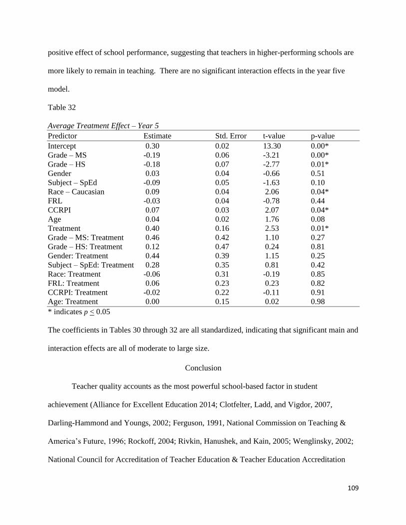
109
positive effect of school performance, suggesting that teachers in higher-performing schools are
more likely to remain in teaching. There are no significant interaction effects in the year five
model.
Table 32
Average Treatment Effect – Year 5
Predictor Estimate Std. Error t-value p-value
Intercept 0.30 0.02 13.30 0.00*
Grade – MS -0.19 0.06 -3.21 0.00*
Grade – HS -0.18 0.07 -2.77 0.01*
Gender 0.03 0.04 -0.66 0.51
Subject – SpEd -0.09 0.05 -1.63 0.10
Race – Caucasian 0.09 0.04 2.06 0.04*
FRL -0.03 0.04 -0.78 0.44
CCRPI 0.07 0.03 2.07 0.04*
Age 0.04 0.02 1.76 0.08
Treatment 0.40 0.16 2.53 0.01*
Grade – MS: Treatment 0.46 0.42 1.10 0.27
Grade – HS: Treatment 0.12 0.47 0.24 0.81
Gender: Treatment 0.44 0.39 1.15 0.25
Subject – SpEd: Treatment 0.28 0.35 0.81 0.42
Race: Treatment -0.06 0.31 -0.19 0.85
FRL: Treatment 0.06 0.23 0.23 0.82
CCRPI: Treatment -0.02 0.22 -0.11 0.91
Age: Treatment 0.00 0.15 0.02 0.98
* indicates p < 0.05
The coefficients in Tables 30 through 32 are all standardized, indicating that significant main and
interaction effects are all of moderate to large size.
Conclusion
Teacher quality accounts as the most powerful school-based factor in student
achievement (Alliance for Excellent Education 2014; Clotfelter, Ladd, and Vigdor, 2007,
Darling-Hammond and Youngs, 2002; Ferguson, 1991, National Commission on Teaching &
America’s Future, 1996; Rockoff, 2004; Rivkin, Hanushek, and Kain, 2005; Wenglinsky, 2002;
National Council for Accreditation of Teacher Education & Teacher Education Accreditation

110
Council, 2010). Highly effective teachers generate cumulative positive effects on student
learning, and close learning deficits and the achievement gaps found in the literature amongst
socio-economically and racially-diverse students (Nye, Konstantopoulos, & Hedges, 2004;
Sanders & Horn, 1994; Sanders & Rivers, 1996; Wright, Horn, & Sanders, 1997).
With the importance of high-quality classroom educators come the challenges of
developing, retaining, and supporting them. Factors such as increased demand due to policy
initiatives and student enrollment are constrained by the decreasing numbers of teacher
candidates completing education programs and salaries that lag behind the entry level salaries in
other professions. School districts are further incented to focus on retaining the teachers they
hire, as attrition costs are at least 30% of the leaving employee’s salary (Mulhere, 2017). As
schools and districts work to retain high-quality teachers, EPPs strive to ensure teacher
candidates are trained to handle the multi-dimensional demands of serving in the classroom.
Federal and state mandates have been in place over the past fifty years to address teacher quality
and preparation programs, and accreditation agencies have long advocated for standardized
pedagogical preparation and practices that provide high levels of pedagogy, content knowledge,
and experiential learning.
Despite mandates, new levels of accountability, and the establishment of EPP standards,
concerns have been raised that EPPs are still inadequately preparing pre-service teachers for
today’s classroom. As many as one-quarter of beginning teachers feel they lack the pedagogy or
content mastery to be effective educators (USDOE, 2013). There is a lack of research showing
the relationship between pre-service preparation, teacher quality, and student learning, further
complicating the debate on the components of effective teacher preparation models (Glazerman,
Mayer, & Decker, 2006; Walsh, 2001).

111
Pre-service programs, such as GSU’s CREST-Ed and NET-Q, are answering the call for
ensuring aspiring teachers are not only ready to enter the classroom but receive continued
support beyond hiring. Both programs feature specialized professional learning partnerships
between the university and participating schools that result in increased integration and relevance
of clinical and academic coursework, research opportunities rooted in schools, and interactions
between mentor teachers and supervising university faculty (Levine, 2006). Other features of the
programs include strong mentor training, year-long pre-service teacher residencies, living stipend
for residents, and TIP-AAR.
The overall goal of this study was to examine the impact of teacher residency programs,
such as NET-Q and CREST-Ed, as well as individual- and school level characteristics on
increasing one-, three-, and five-year retention rates of beginning teachers. Multilevel logistic
regression was used to identify models that captured the individual- and school-level predictors
that best inform teacher retention and to estimate propensity scores for each control and
treatment participate. Once propensity scores were generated, full matching was used to match
nontreated participants to treated ones based on probabilities of receiving treatment. The ATT
and ATE were computed to determine whether beginning teachers who were participants in the
CREST-Ed and NET-Q residency programs remained in teaching at a higher rate than non-
participants.
Teacher retention research suggests that a variety of individual (age, gender,
race/ethnicity, content area taught) and school-level characteristics (percentage of minority
students, percentage of students on free and/or reduced lunch, grade band, CCRPI score, school
climate) are associated with beginning teacher attrition rates. Results of the multilevel logistic
regression confirmed the significance of factors such as grade level, gender, content area subject

112
taught, and school performance in informing teacher retention. None of these variables were
significant in all three models, suggesting that the factors influencing a teacher retention are
dynamic over time and may change as teachers gain more classroom experience. While not
statistically significant predictors in any of the models used to generate propensity scores, factors
such as teacher age, teacher race/ethnicity, school climate, and school socioeconomic
demographics can also inform teacher retention in an aggregate form.
Pre-service teacher research also indicates the importance of programs featuring year-
long clinical experiences that provide aspiring teachers with practical, skill-oriented, diverse
experiences that connect theory and current practices. Programs such as CREST-Ed and NET-Q
also provide pre-service teachers with opportunities to analyze and reflect on their experiences
and learning with mentor teachers, clinical supervisors, and their peers. Optimal full matching
was used to measure whether CREST-Ed and NET-Q residents had higher retention rates than
their matched peers. The results supported the hypothesis that the program participants had
significantly higher one-, three-, and five-year retention rates than the non-participating teachers.
Both the ATT and the year one and five ATE models indicate the effectiveness of the CREST-Ed
and NET-Q programs in training prospective teachers and that, on average, program participation
is a beneficial experience for residents as measured by long-term employment as an educator.
The ATT had a notable effect size for the year five model, which may indicate that the signature
components of CREST-Ed and NET-Q programs, such as the year-long residency and TIP-AAR,
have a long-term impact on teacher quality. While age, teacher race, school socioeconomic
composition, school performance, and subject taught served as significant predictors of teacher
retention, teacher race was the only predictor significant in all three ATE models. All three
models indicated Caucasian teachers are more likely to remain in teaching than minority

113
teachers. Beginning younger teachers were more likely to remain in teaching beyond the first
year. Teachers are more likely to remain in teaching beyond year three in more affluent schools
and beyond year five in high performing schools. Special education teachers are less likely to
remain in teaching beyond three years and secondary teachers beyond five years. All significant
main effect findings were consistent with teacher retention literature.
The study contributes to scholarly knowledge in the area of teacher residency programs,
and on factors that are associated with beginning teacher retention. In addition, the research
serves to bridge the current gap in literature connecting pre-service program effectiveness to
teacher retention. This outcome has educational policy implications, as it suggests the
importance of EPPs in ensuring teachers have the skills, knowledge, and abilities beyond the
hiring process and well into their careers. It is essential for accrediting agencies, Colleges of
Education, state and federal lawmakers, teacher advocacy organizations, school districts, and
state and federal departments of education to continue and expand the dialog regarding the
factors that support teacher retention and the pre-service and induction programs that need to be
in place to ensure every classroom has a supported, quality teacher. The study also informs the
need for designing meaningful year-long clinical experiences, opportunities for pre-service
teachers to engage in action research, and continued professional learning once the pre-service
teacher enters the classroom. Future research can potentially use this work as a framework by
which other pre-service interventions can be evaluated. This research serves to inform how the
NET-Q and CREST-Ed grants awarded to GSU by USDOE are performing relative to their goals
of increasing the quality and number of highly qualified teachers committed to Georgia high
needs schools and ensuring new teachers receive the support to remain in the classroom. Due to

114
the longitudinal nature of the study, program impact was incrementally analyzed over a five year
span.
This dissertation has a few key limitations and several areas for future research. First, a true
experimental design could not be used in the study as it requires that participants be randomly
assigned to treatment and comparison groups. This condition could not be met in this research
study because participation in the treatment group was based on student decision to enroll in the
CREST-Ed and NET-Q programs. As a result, causal inferences are difficult to support, and
threats to internal validity are increased.
The treatment sample consisted of a small group of pre-service teachers who participated in
GSU’s CREST-Ed or NET-Q educator preparation programs. To find effects and make the study
generalizable to other populations, the study would need to be replicated with a larger population
of teachers exposed to comparable programs. Another avenue for future research may be the
continuation of this study in a few years, enabling a larger sample size to build for the year five
model. The negligible effect size for two models and the small effect size for the year five
model further heightens concern the study may not be generalizable to other populations. Future
studies may also consider adding more covariates to the models or another form of PSA, echoing
Gao and Fraser’s (2015) overall desire for additional research on the circumstances PSAs should
be preferred over conventional regression methods as it relates to selection bias and when certain
PSAs should be utilized. There is also a need for studies to add to the review of literature on
research circumstances when PSA would be superior to other regression models, especially when
the data requires multilevel analysis.
There are also opportunities for mixed methods study. The CPI report only captures
information for staff working in public K-12 LEAs in Georgia; there may be treatment

115
participants who transferred to either a private Georgia school or an institution outside of
Georgia. During interviews of NET-Q program graduates currently teaching, conducted by GSU
researchers, former residents established their connection to students and the ability to witness
their holistic growth as reasons for staying in teaching. Graduates also noted TIP-AAR
experience a program strength, with some continuing to utilize action research as a component of
their instructional practices. The year-long residency was also cited as an important program
component that provided them with a classroom knowledge and comfort level that varied from
other new teachers. However, efforts to interview graduates not currently in teacher positions
have been unsuccessful. (R. Hendrick, personal communication, February 22, 2019). Continued
opportunities to follow-up with CREST-Ed and NET-Q residents would produce rich and deep
information on whether residents left the teaching profession, the reasons for leaving, and the
impact of the program on their teaching practices.

116
References
Alliance for Excellent Education (2014). On the path to equity: Improving the effectiveness of
beginning teachers. Retrieved from https://all4ed.org/wp-
content/uploads/2014/07/PathToEquity.pdf.
Buren, S., Brand, J., Groothuis-Oudshoorn, C., & Rubin, D. (2006). Fully conditional
specification in multivariate imputation. Journal of Statistical Computation and
Simulation, 76(12), 1049-1064.
Clotfelter, C., Ladd, H., & Vigdor, 2007. Teacher credentials and student achievement in high
school: A cross-subject analysis with student fixed effects. Economics of Education
Review, 26(6), 673-782.
Cohen, J. (1988). Statistical power analysis for the behavioral sciences. Hillsdale, NJ:
Lawrence Erlbaum.
Cuong, N. (2013). Which covariates should be controlled in propensity score matching?
Evidence from a simulation study. Statistica Neerlandica, 67(2), 169-180.
Darling-Hammond, L., & Youngs, P. (2002). Defining “highly qualified teachers”: What does
scientifically-based research actually tell us? Educational Researcher, 31(9), 13-25.
Diamond, A. & Sekhon, J. (2013). Genetic matching for estimating causal effects: A general
multivariate matching method for achieving balance in observational studies. The
Review of Economics and Statistics, 95(3), 932-945.
Dziak, J., Coffman, D., Lanza, S., & Li, R. (2012). Sensitivity and Specificity of Information
Criteria. Retrieved from https://www.methodology.psu.edu/files/2019/03/12-119-
2e90hc6.pdf.
Ferguson, R. (1991). Paying for public education: New evidence on how and why money
matters. Harvard Journal on Legislation, 29(2), 465-98.
Georgia Department of Education (2018). Data Collections – FY2018. Retrieved from
https://www.gadoe.org/Technology-Services/Data-
Collections/Documents/DC_Conf_DataColl/FY2018/CPI%20101%20-
%20Basics%20of%20CPI%20Personnel%20Reporting.pdf.

117
Georgia Department of Education (2019a). College and career ready performance index.
Retrieved from http://www.gadoe.org/CCRPI/Pages/default.aspx.
Georgia Department of Education (2019b). Free and reduced price meal eligibility. Retrieved
from https://oraapp.doe.k12.ga.us/ows-bin/owa/fte_pack_frl001_public.entry_form.
Glazerman, S., Mayer, D., & Decker, P. (2006). Alternative routes to teaching: The impacts
of Teach for America on student achievement and other outcomes. Journal of Policy
Analysis and Management, 25(1), 75–96.
Governor’s Office of Student Achievement (2019). Downloadable data. Retrieved from
https://gosa.georgia.gov/downloadable-data.
Govindasamy, P. & Olmos, A. (2015). Introduction to optimalpostmatch package in R.
Retrieved from file:///C:/Users/BNC/Downloads/Optmatch_AEA_2015%20(2).pdf.
Guo, S. & Fraser, M. (2015). Propensity score analysis. Thousand Oaks, California: SAGE
Publications.
Ho, D., Imai, K., King, G., Stuart, E. (2007). Matching as nonparametric preprocessing for
reducing model dependence in parametric causal inference. Political Analysis, 15, 199-
236.
Ho, D., Imai, K., King, G., Stuart, E. (2011). MatchIt: Nonparametric preprocessing for
parametric causal inference. Retrieved from https://r.iq.harvard.edu/docs/matchit/2.4-
20/matchit.pdf.
Kelcey, B. (2011). Propensity score matching within versus across schools. Retrieved from
https://eric.ed.gov/?id=ED518897.
Leite, W. (2017). Practicing propensity score methods in using R. Thousand Oaks: SAGE
Publications.

118
Levine, A. (2006). Educating school teachers. Retrieved from
http://edschools.org/pdf/Educating_Teachers_Report.pdf.
Mass, C. & Hox, J. (2005). Sufficient sample sizes for multilevel modeling. Retrieved from
http://joophox.net/publist/methodology05.pdf.
McFadden, D. (1974). Conditional logit analysis of qualitative choice behavior. Retrieved from
https://eml.berkeley.edu/~mcfadden/travel/ch5.pdf.
Mulhere, K. (2017). People think teachers are underpaid – Until you tell them how much
teachers earn. Retrieved from http://time.com/money/4900091/teachers-average-salary-
underpaid-poll/.
National Commission on Teaching and America’s Future (1996). What matters most: Teaching
for America’s Future. Retrieved from https://nctaf.org/wp-
content/uploads/WhatMattersMost.pdf.
National Council for Accreditation for Teacher Education & Teacher Education Accreditation
Council (2010). Report and recommendation of the NCATE/TEAC Design Team to Our
Respective Boards of Directors. Retrieved from
http://caepnet.org/~/media/Files/caep/about/designteamreport.pdf?la=en
Nye, B., Konstantopoulos, S., & Hedges, L. (2004). How large are teacher effects? Educational
Evaluation and Policy Analysis, 26(4), 237-57.
Rivkin, S., Hanushek, E., & Kain, J. (2005). Teachers, schools, and academic achievement.
Econometrica, 73(2), 417-458.
Rockoff, J. (2004). The impact of individual teachers on student achievement: Evidence from
panel data. American Economic Review, 94(2), 247-252.
Sanders, W. & Horn, S. (1994). The Tennessee value-added assessment system (TVAAS):
Mixed-model methodology in education assessment. Journal of Personnel Evaluation in
Education, 8(3), 299-311.

119
Sanders, W. & Rivers, J. (1996). Cumulative and residual effects of teachers on student
academic achievement: Research progress report. Retrieved from
http://www.cgp.upenn.edu/pdf/Sanders_Rivers-TVASS_teacher%20effects.pdf.
Shea, C. (1996). Psychologists debate accuracy of “significance test.” Chronicle of
Higher Education, 42(49), A12, A16.
U.S. Department of Education, Institute of Education Science and What Works Clearinghouse
(2013). What works clearinghouse: Procedures and standards handbook. Retrieved
from
https://ies.ed.gov/ncee/wwc/Docs/referenceresources/wwc_procedures_v3_0_standards_
handbook.pdf.
U.S. Department of Education, Institute of Education Sciences, National Center for Education
Statistics (2013). Schools and Staffing Survey (SASS): Public School Teacher Data File,
2011–12. Retrieved from
https://nces.ed.gov/surveys/sass/tables/sass1112_2016001_t1s.asp.
Vacha-Haase, T. & Thompson, B. (2004). How to estimate and interpret various effect
sizes. Journal of Counseling Psychology, 51(4) 473-481.
Walsh, K. (2001). Teacher certification reconsidered: Stumbling for quality. Retrieved from
https://www.nctq.org/dmsView/Teacher_Certification_Reconsidered_Stumbling_for_Qu
ality_NCTQ_Report.
Wenglinsky, H. (2002). How schools matter: The link between teacher classroom practices and
student academic performance. Retrieved from
https://epaa.asu.edu/ojs/article/view/291.
Wilkinson, L., & APA Task Force on Statistical Inference. (1999). Statistical methods in
psychology journals: Guidelines and explanations. Retrieved from http://www.apa.org/
journals/amp/amp548594.html].
Wright, S., Horn, S., & Sanders, W. (1997). Teacher and classroom context effects on student
achievement: Implications for teacher evaluation. Journal of Personnel Evaluation in
Education, 11(1), 57-67.

120
APPENDICES
Appendix A
List of CCRPI Indicators (GaDOE, 2018a)
Content Mastery
• English Language Arts achievement
• Mathematics achievement
• Science achievement
• Social studies achievement
Progress
• English Language Arts growth
• Mathematics growth
• Progress towards ELL proficiency
Closing Gaps
• Meeting achievement improvement targets
Readiness
• Elementary and Middle School
o Literacy: % of students demonstrating reading comprehension at or above the
midpoint of Lexile stretch bands
o Student attendance: percent of students absent less than 10% of enrolled days
o Beyond the core: students earning a passing score in fine arts, world
language, health/physical education (middle school), or career exploratory
(middle school)
• High School (each indicator weighted at 20%)

121
o Literacy
o Student attendance
o Accelerated enrollment: % of seniors earning credit for dual enrollment,
Advanced Placement, or International Baccalaureate courses
o Pathway completion: % of seniors completing an advanced academic, CTAE,
fine arts, or world language pathway
o College and career readiness: % of seniors meeting one or more of the
following:
▪ entering a Georgia public university or technical college without
needing remediation;
▪ readiness score on the ACT, SAT, two or more AP exams, or two or
more IB exams;
▪ passing an end of pathway assessment;
▪ completing a work-based learning program
Graduation Rate (high schools only)
• 4-year adjusted cohort graduation rate (weighted at 66.67%)
• 5-year adjusted cohort graduation rate (weighted at 33.33%)

122
Appendix B
List of Education Preparation Providers Approved by the Georgia Professional Standards
Commission
Initial Certification Programs (GaPSC, 2018b)
Traditional Programs Alternative Programs
Albany State University
Armstrong State University
Augusta College
Berry College
Brenau University
Brewton-Parker College
Clark Atlanta University
Clayton State University
College of Coastal Georgia
Columbus State University
Covenant College
Dalton State College
Emmanuel College
Fort Valley State University
Georgia College and State University
Georgia Gwinnett College
Georgia Southern University
Georgia Southwestern State University
Georgia State University
Gordon State College
Kennesaw State University
Lagrange College
Mercer University
Middle Georgia State University
Paine College
Piedmont College
Point University
Reinhardt University
Savannah State University
Shorter University
Spelman College
Thomas University
Toccoa Falls College
Truett-McConnell University
University of Georgia
University of North Georgia

123
Traditional Programs
University of West Georgia
Valdosta State University
Wesleyan College
Young Harris College
Alternative Programs
Central Savannah River Area RESA
Clayton County Public Schools
DeKalb County Schools
First District RESA
Fulton County Schools
Georgia Charter Schools Association
Georgia Teaching Fellows
Griffin RESA
Gwinnett County Public Schools
Metro RESA
Middle Georgia RESA
Northeast Georgia RESA
Northwest Georgia RESA
Oconee RESA
Okefenokee RESA
Pioneer RESA
Southwest Georgia RESA
Teach for America Metro Atlanta
Technical College System of Georgia
West Georgia RESA

124
Appendix C
Sample R Coding for Matching Analysis
#load the dataset
file.choose()
library(foreign)
dataset<-read.spss("C:\\Users\\BNC\\Documents\\Dissertation 2018\\1.26\\Year One 1.29b Impu
ted.sav", to.data.frame = TRUE)
# creating dummy variables
dataset$Group.f<-factor(dataset$Group)
is.factor(dataset$Group.f)
dataset$Group.f[1:15]
dataset$Grade.f<-factor(dataset$Grade)
is.factor(dataset$Grade.f)
dataset$Grade.f[1:15]
dataset$Gender.f<-factor(dataset$Gender)
is.factor(dataset$Gender.f)
dataset$Gender.f[1:15]
dataset$Subject.f<-factor(dataset$Subject)
is.factor(dataset$Subject.f)
dataset$Subject.f[1:15]
dataset$Race.f<-factor(dataset$Race)
is.factor(dataset$Race.f)
dataset$Race.f[1:15]
dataset$Y1Outcome.f<-factor(dataset$Y1Outcome)
is.factor(dataset$Y1Outcome.f)
dataset$Y1Outcome.f[1:15]
#standardized continuous predictors
dataset$FRL=(dataset$FRL-mean(dataset$FRL))/sd(dataset$FRL)
dataset$CCRPI=(dataset$CCRPI-mean(dataset$CCRPI))/sd(dataset$CCRPI)
dataset$Age=(dataset$Age-mean(dataset$Age))/sd(dataset$Age)
dataset$Climate=(dataset$Climate-mean(dataset$Climate))/sd(dataset$Climate)
dataset$Minority=(dataset$Minority-mean(dataset$Minority))/sd(dataset$Minority)
#create formula of multilevel logistic regression model
library(lme4)

125
ps.formula<-dataset$Group.f+dataset$Grade.f+dataset$FRL+dataset$CCRPI+dataset$Climate+d
ataset$Gender.f+dataset$Race.f+dataset$Age+dataset$Subject.f+(1|dataset$School)
print(ps.formula)
#fit a multilevel model with a random intercept
ps.model<-glmer(ps.formula, data = dataset, family = binomial, glmerControl(optimizer="bobyq
a", optCtrl = list(maxfun = 150000)))
#extract the model estimated propensity scores
dataset$ps<-fitted(ps.model)
with(dataset, by(dataset$ps,dataset$Group.f, summary))
dataset$logitPScores<-log(fitted(ps.model)/(1-fitted(ps.model)))
summary(dataset$logitPScores)
#model fit with McFadden’s R2
nullmod<-glm(dataset$Group.f~1,family=binomial)
1-logLik(ps.model)/logLik(nullmod)
#evaluate common support with boxplot
library(lattice)
par("mar")
par(mar=c(1,1,1,1))
boxplot(dataset$logitPScores~dataset$Group.f, data= dataset)
#Perform optimal full matching
library(MatchIt)
library(optmatch)
fullMatching<-matchit(ps.formula, distance = “linear.logit”, data = dataset, method = "full", cali
per=0.25)
#diagnose covariate balance
Summary(fullMatching, standardize=T)
plot(fullMatching)
#Estimate Treatment Effects with optimal full matched data using regression
library(survey)
data.fullMatching<-match.data(fullMatching)
data.fullMatching$Grade<-scale(as.numeric(data.fullMatching$Grade==1), scale = F)
data.fullMatching$Gender<-scale(as.numeric(data.fullMatching$Gender==1),scale=F)
data.fullMatching$Subject<-scale(as.numeric(data.fullMatching$Subject==1),scale=F)
data.fullMatching$Race<-scale(as.numeric(data.fullMatching$Race==1),scale=F)
data.fullMatching$Outcome<-as.numeric(data.fullMatching$YOutcome==1)
data.fullMatching$treated<-as.numeric(data.fullMatching5$Group==1)

126
design.fullMatching<-svydesign(ids = ~School, nest = T, weights = ~weights, data = data.fullMa
tching)
#fit ATT & ATE regression model
model.fullMatchingATT<-svyglm(Outcome~treated, design.fullMatching, family=gaussian())
summary(model.fullMatchingATT)
model.fullMatchingATE<-svyglm(formula = Outcome~(Grade+Gender+Subject+Race+FRL+C
CRPI+Age+Climate)*treated, design.fullMatching, family=gaussian())
summary(model.fullMatchingATE)
#post matching analysis
library(effsize)
cohen.d(data.fullMatching$Group~data.fullMatching$YOutcome, data = data.fullMatching)
chi.data=table(data.fullMatching$Group.f, data.fullMatching$YOutcome)
print(chisq.test(chi.data))