European Journal of Control 43 (2018) 46–56

Contents lists available at ScienceDirect

European Journal of Control

journal homepage: www.elsevier.com/locate/ejcon

Regional stability and stabilization of a class of linear hyperbolic

systems with nonlinear quadratic dynamic boundary conditions

André F. Caldeira

a , b , 1 , ∗, Christophe Prieur c , Daniel Coutinho

d , Valter J.S. Leite

e

a Graduate Program on Automation and Systems Engineering, UFSC, PO BOX 476, 88040-900 Florianópolis, SC, Brazil b Grenoble Image Parole Signal Automatique (GIPSA-lab), Grenoble F-380 0 0, France c University Grenoble Alpes, CNRS, Grenoble INP, GIPSA-lab, Grenoble F-380 0 0, France d Department of Automation and Systems, UFSC, Florianópolis, SC, PO BOX 476, 88040-900, Brazil e Department of Mechatronics Engineering, CEFET-MG – Campus Divinópolis, R. Álvares Azevedo, 400, 35503-822 MG, Brazil

a r t i c l e i n f o

Article history:

Received 3 April 2017

Revised 8 April 2018

Accepted 20 May 2018

Available online 26 May 2018

Recommended by D. Melchor-Aguilar

Keywords:

Dynamic boundary conditions

Poiseuille flow

Linear hyperbolic systems

Robust control

LMIs

a b s t r a c t

This paper addresses the boundary control problem of fluid transport in a Poiseuille flow taking the ac-

tuator dynamics into account. More precisely, sufficient stability conditions are derived to guarantee the

exponential stability of a linear hyperbolic differential equation system subject to nonlinear quadratic dy-

namic boundary conditions by means of Lyapunov based techniques. Then, convex optimization problems

in terms of linear matrix inequality constraints are derived to either estimate the closed-loop stability

region or synthesize a robust control law ensuring the local closed-loop stability while estimating an ad-

missible set of initial states. The proposed results are then applied to application-oriented examples to

illustrate local stability and stabilization tools.

© 2018 European Control Association. Published by Elsevier Ltd. All rights reserved.

t

p

f

t

d

e

t

s

[

l

d

s

m

m

L

1. Introduction

In industrial processes, a large variety of physical systems is

governed by hyperbolic partial differential equations (PDEs) such

as hydraulic networks [4,21] and gas devices [11,12] . In particular,

fluid transport is often modeled by balance laws (or conservation

laws when additive and dissipative terms are disregarded) which

are hyperbolic PDEs normally used to express the fundamental

dynamics of open conservative systems. However, infinite dimen-

sional systems introduce variable time-delays making the closed-

loop control much more challenging and, moreover, distributed

measurements and actuators are not usually available. As a conse-

quence, it is more common that actuators and measurements are

located at the boundaries which is desired in practical applications

as, for instance, in the references previously cited. In addition, a

large number of numerical techniques based on finite-dimensional

∗ Corresponding author at: Graduate Program on Automation and Systems Engi-

neering, UFSC, Grenoble PO BOX 476, 88040-900 Florianópolis, SC, Brazil.

E-mail addresses: caldeiraaf@gmail.com (A.F. Caldeira), christophe.prieur@gipsa-

lab.fr (C. Prieur), coutinho@das.ufsc.br (D. Coutinho), valter@ieee.org (V.J.S. Leite). 1 A. F. Caldeira was pursuing a doctoral degree in the Graduate Program on Au-

tomation and Systems Engineering, UFSC, and École Doctorale Electronique, Elec-

trotechnique, Automatique, Traitement du Signal, Univ. Grenoble Alpes.

t

s

t

p

i

s

a

https://doi.org/10.1016/j.ejcon.2018.05.003

0947-3580/© 2018 European Control Association. Published by Elsevier Ltd. All rights rese

ools, which are often used to the stability analysis of PDE systems,

rovides only approximate solutions.

On the other hand, Lyapunov theory has been largely applied

or several decades to deal with the stability analysis and con-

rol design of finite dimensional systems described by ordinary

ifferential equations (ODEs) [37] . In the particular case of lin-

ar dynamical systems, a large number of stability and stabiliza-

ion results are cast in terms of linear matrix inequality (LMI) con-

traints [6] , which are numerically solved using dedicated software

30] . The LMI framework is a powerful tool for linear and non-

inear finite-dimensional systems, since it can deal with a large

iversity of control and systems theory problems such as robust

tability, domain of attraction estimation, input-to-output perfor-

ance, state or dynamic output-feedback control, and state esti-

ation (see [6,7,13,18,24,32] among other references). As a result,

MIs have been successfully applied in a wide diversity of con-

rol oriented applications as, for instance, wind turbine operation,

atellite attitude regulation, turbo-charged combustion engine con-

rol and bioprocess control and estimation [19,31] .

In the context of infinite dimensional systems, the stability

roblem of boundary control for first-order hyperbolic systems us-

ng quadratic strict Lyapunov functions was more recently stated;

ee, for instance, [15,16,33] . A common assumption in most of

vailable results is that the boundary action is faster than the wave

rved.

A.F. Caldeira et al. / European Journal of Control 43 (2018) 46–56 47

t

t

a

t

c

b

t

p

d

a

h

c

t

c

p

w

t

i

a

d

i

j

t

fi

a

b

s

v

n

b

i

t

s

i

l

r

d

i

t

a

p

t

a

t

e

t

i

l

t

t

l

t

b

s

m

l

i

T

t

S

s

I

d

d

S

X

a

c

i

s

e

a

f

2

�

fi

l

∂

w

v

d

�

t

w

i

A

f

0

R

c

N

p

m

t

R

t

λ

a

ξ

T

ξ

y

d{

w

ξ

a

d

v

s

a

c

t

ravel making possible to establish a static relationship between

he control input and the boundary condition. However, there are

pplications where the dynamics associated to the boundary con-

rol action cannot be neglected as, for instance, in the temperature

ontrol of an airflow in a heating column. To deal with dynamic

oundary actions, the infinite-dimensional system discretization

ogether with the use of finite-dimensional tools are often em-

loyed. On the other hand, several approaches considering infinite-

imensional based techniques have been recently proposed. To cite

few, some sufficient conditions for the exponential stability of

yperbolic systems with linear time invariant dynamic boundary

onditions were proposed in [10] , the backstepping technique for

he boundary control of hyperbolic and time-delayed systems was

onsidered in [28] , the dynamic boundary stabilization of linear

arameter-varying (LPV) hyperbolic systems using the LMI frame-

ork was studied in [12] , the problem of stability analysis and con-

rol synthesis for first-order hyperbolic linear PDEs over a bounded

nterval with spatially varying coefficients was the focus of [29] ,

nd a multimodel approach with a bilinear matrix inequality to

eal with the stability of a hyperbolic system representing the flow

n a open channel was proposed in [23] . It turns out that the ma-

ority of the latter references consider only dynamic boundary ac-

ions described by linear differential equations.

This paper addresses the boundary stabilization of uncertain

rst-order hyperbolic systems with boundary actions governed by

n uncertain nonlinear quadratic differential equation. It should

e emphasized that the class of quadratic systems can describe

tate-space models containing quadratic nonlinearities in the state

ariables and bilinear terms involving the state and control sig-

al. Moreover, this class of systems can represent a large num-

er of processes such as distillation and heating columns [10,25] ,

nduction motors [3] and DC–DC converters [35] , which has at-

racted recurring interest of the control practitioners; see, for in-

tance, [1,2,17,36] and references therein. Notice, in the context of

nfinite dimensional systems, that boundary actions are often non-

inear as, for instance, in the geometric average particle volume

egulation of plug-low reactors, flow regulation in open channels

elimited by overflow spillways and the vibration rejection in flex-

ble marine risers [14,16,26] . In particular, local boundary stabiliza-

ion conditions for the coupled linear first-order hyperbolic system

nd nonlinear quadratic dynamic boundary actuation are in this

aper proposed in terms of a finite set of LMI constraints based on

he Lyapunov stability theory. The local stability is characterized in

regional context, that is, bounded initial states will imply that

he state trajectories remain bounded and they converge to the

quilibrium point as the time goes to infinity. Hence, an optimiza-

ion problem is proposed for the boundary feedback control design

n order to determine a quadratic boundary state feedback control

aw that maximizes the set of admissible boundary initial condi-

ions while guaranteeing the stability of the coupled ODE-PDE sys-

em.

The remaining of this paper is organized as follows. The prob-

em of interest is stated in Section 2 . Then, Section 3 presents

he main stability results for uncertain first-order linear hyper-

olic system subject to nonlinear boundary conditions. Next, the

tability results are adapted in Section 4 to control synthesis by

eans of an appropriate similarity transformation where a stabi-

izing nonlinear boundary state feedback control law is designed

n order to maximize the region of admissible initial conditions.

hen, Section 5 provides two application-based examples in order

o demonstrated the potentials of the proposed approach. Finally,

ection 6 ends the paper giving some concluding remarks.

Notation: R

+ = [0 , + ∞ ) , R

n is the n -dimensional Euclidean

pace, R

m ×n is the set of m × n real matrices with real entries,

n in the n × n identity matrix, 0 n is the n × n zeros matrix and

iag{ · · · } denotes a block-diagonal matrix. For a real matrix S , S ′

enotes its transpose, He{ S } stands for S + S ′ , and S > 0 means that

is symmetric and positive-definite. For two polytopes X and Y,

× Y denotes the meta-polytope obtained by cartesian product

nd V(X ) is the set of all vertices of X . For a vector ξ ∈ R

n , the k -

omponent of ξ is denoted by ξ ( k ) . The usual Euclidian norm in R

n

s denoted by ‖ · ‖ , whereas the set of all functions φ : (0 , L ) → R

n

uch that ∫ L

0 φ(x ) ′ φ(x ) dx < ∞ is denoted by L 2 ((0 , L ) ; R

n ) that is

quipped with the norm ‖ · ‖ L 2 ((0 ,L ) ;R n ) . Given a topological set J ,

nd an interval I in R

+ , the set C 0 (I, J ) is the set of continuous

unctions φ : I → J .

. Problem statement

Let n be a positive integer, � an open non-empty set of R

n and

a non empty convex set of R

n δ . Consider the general class of

rst-order uncertain hyperbolic systems of order n defined as fol-

ows:

t ξ(t, x ) + �(δ) ∂ x ξ(t, x ) = 0 , t ∈ R

+ , x ∈ [0 , L ] , (1)

here ξ : R

+ × [0 , L ] → �, δ ∈ � is a bounded sufficiently smooth

ector function of time; ∂ t and ∂ x represent (first order) partial

erivatives with respect to time and space, respectively; �(δ) :

→ R

n ×n is a diagonal and continuous matrix function (called

he characteristic matrix), i.e., �(δ) = diag { λ1 (δ) , λ2 (δ) , . . . , λn (δ) }ith λi ( δ) being positive continuous functions, for all δ ∈ � and

= 1 , . . . , n .

ssumption 1. The diagonal elements of �(δ) ∈ R

n ×n satisfy the

ollowing inequalities for all δ ∈ �:

< λ1 (δ) < · · · < λn (δ) .

emark 1. Assumption 1 implies that system (1) has only positive

onvecting speeds, however it does not add any loss of generality.

ote that, for first order hyperbolic systems with both negative and

ositive convecting speeds, there always exists a variable transfor-

ation to obtain a system as in (1) satisfying Assumption 1 (see

he beginning of proof of Theorem 1 in [10] , or Page 7 of [34] or

emark 1 of [12] or Remark 3 of [11] ). In particular, consider sys-

em (1) with the diagonal elements of �( δ) ordered as follows

1 (δ) < · · · < λm

(δ) < 0 < λm +1 (δ) < · · · < λn (δ) , ∀ δ ∈ �,

nd let ξ : R

+ × [0 , L ] → � ∈ R

n be partitioned as

(t, x ) =

[ξ−(t, x ) ξ+ (t, x )

], ξ− ∈ R

m , ξ+ ∈ R

n −m .

hen, applying the transformation

˜ (t, x ) =

[ξ−(t, L − x )

ξ+ (t, x )

]

ields a system as in (1) with only positive convection speeds.

Associated with (1) , consider the following nonlinear quadratic

ynamic boundary action:

˙ ξin (t) = A (ξin (t) , δ) ξin (t) + B (ξin (t ) , δ) u (t ) ,

u (t) = G (ξin (t)) ξin (t) + Kξout (t) , (2)

here

in (t) = ξ(t , 0) , ξout (t ) = ξ(t, L ) (3)

re the boundary conditions of (1) interconnecting the boundary

ynamics of (1) with (2) , ξin ∈ ⊂ R

n and ξout ∈ R

n are the state

ectors of the dynamic boundary condition at x = 0 and x = L, re-

pectively, and assumed to be measurable, u (t) ∈ R

n u is the bound-

ry control input, is compact region of the boundary state-space

ontaining ξin = 0 and to be specified later in this paper. Notice

o ease the presentation that the system and boundary dynamics

48 A.F. Caldeira et al. / European Journal of Control 43 (2018) 46–56

3

m

y

f

d

V

w

i

t

f

V

b

V

w

m

m

t

t

ε

m

f

V

f

O

s

D

P

R

f

V

N

c∫

uncertainties are merged into the vector δ, i.e., the elements of δcomprise both system and boundary dynamics modeling errors.

Further, K ∈ R

n u ×n is a real constant matrix and A (·) ∈ R

n ×n ,

B (·) ∈ R

n ×n u , G (·) ∈ R

n u ×n are affine matrix functions on their ar-

guments, that is:

[A (ξin , δ) B (ξin , δ)

]= [ A 0 B 0 ] +

n ∑

i =1

ξin (i ) [ A i B i ]

+

n δ∑

j=1

δ( j)

[A j B j

], (4)

G (ξin ) = G 0 +

n ∑

i =1

ξin (i ) G i , (5)

with A i , B i , and G i , i = 0 , 1 , . . . , n, and A j , B j , j = 1 , . . . , n δ, being

given constant real matrices with appropriate dimensions. It is as-

sumed that the pair ( A 0 , B 0 ) is stabilizable and the unforced system

of (2) is allowed to be unstable.

In addition, the initial conditions of the coupled PDE-ODE sys-

tem of (1) and (2) , namely

ξ(0 , x ) = ξ(x ) and ξin (0) = ξin , (6)

are assumed to satisfy:

ξ ∈ D 1 and ξin ∈ D 2 , (7)

where the sets D 1 and D 2 are defined as follows

D 1 :=

{ξ ∈ L 2 ((0 , L ) ; R

n ) :

∫ L

0

ξ(x ) ′ ξ(x ) dx ≤ σ

}, (8)

D 2 :=

{

ξin ∈ R

n : ξin ′ P 1 ξin ≤ 1

}

,

with the scalar σ > 0 and the matrix P 1 > 0 defining the sizes of

D 1 and D 2 , respectively. In the particular case of linear dynamic

boundary conditions, that is, when A i , B i , A i and B i are null ma-

trices, for i = 1 , . . . , n, the existence and uniqueness of solutions to

(2) , (3) and (6) for initial conditions satisfying (7) is ensured, see

e.g. [15] . As these solutions may not be differentiable everywhere,

the concept of weak solutions to partial differential equations has

to be used; see [21] and references therein for further details.

In view of the above scenario, this paper is concerned in ob-

taining sufficient conditions to the regional stability and stabiliza-

tion problems for coupled PDE-ODE system of (1) and (2) as stated

below:

P1 For given state feedback gain matrices G ( ξin ) and K ( ξout ) as

defined in (5) , derive stability analysis conditions ensuring

the robust local stability of the coupled PDE-ODE system

while determining a maximized set of initial boundary states

D 2 for a given set D 1 .

P2 Design the state feedback gain matrices G ( ξin ) and K ( ξout )

as defined in (5) , ensuring the robust local stability of the

coupled PDE-ODE system while maximizing the set of initial

boundary states D 2 for a given set D 1 .

Before ending this section, the notion of exponential stability to

be considered in this paper is introduced for the coupled PDE-ODE

system of (1) and (2) .

Definition 1. The coupled PDE-ODE system of (1) and (2) , with ini-

tial conditions ξ and ξin satisfying (7) , is said to be locally robustly

exponentially stable if there exist positive scalars α and β such

that the following holds: (‖ ξin (t) ‖ + ‖ ξ(t, ·) ‖ L 2 ((0 ,L ) ;R n ) )

≤ βe −αt (‖ ξin ‖ + ‖ ξ‖ L 2 ((0 ,L ) ;R n )

),

+

∀ t ∈ R , δ ∈ �. (9)

. Local stability analysis

In this section, it is developed an LMI approach to derive a nu-

erical and tractable solution to the robust regional stability anal-

sis problem P1 as defined in Section 2 . To this end, consider the

ollowing Lyapunov function candidate defined for all continuously

ifferentiable functions ξ : R

+ × [0 , L ] → �:

(ξ) = ξ′ in P 1 ξin +

∫ L

0

e −μx ξ(x ) ′ P 2 ξ(x ) dx, (10)

here P 1 , P 2 ∈ R

n ×n are positive definite diagonal matrices and μs a positive scalar.

Then, evaluating the time derivative of V ( · ) along the solutions

o (1) and (2) with (7) leads to (see, for instance, [16] and [11] for

urther details):

˙ (ξ(t, ·)) = 2 ξin (t) ′ P 1

(A (ξin , δ) + B (ξin , δ) G (ξin )

)ξin (t)

+ 2 ξin (t) ′ P 1 B (ξin , δ) Kξout (t) −[e −μx ξ(t, x ) ′ �(δ) P 2 ξ(t, x )

]x = L x =0

− μ

∫ L

0

e −μx ξ(t, x ) ′ �(δ) P 2 ξ(t, x ) dx

In light of the above and taking (3) into account, ˙ V (ξ(t, ·)) can

e cast as follows:

˙ (ξ(t, ·)) = −m 1 (ξ, δ) + m 2 (ξin , ξout , δ) (11)

here

1 (ξ, δ) = μ

(ξ′

in �(δ) P 1 ξin +

∫ L

0

e −μx ξ(t, x ) ′ �(δ) P 2 ξ(t, x ) dx

),

2 (ξin , ξout , δ) = ξ′ a (ξin , δ) ξa , ξa =

[ξin

ξout

],

(ξin , δ) =

⎡

⎢ ⎢ ⎢ ⎢ ⎣

A (ξin , δ) ′ P 1 +P 1 A (ξin , δ)

+ G (ξin ) ′ B (ξin , δ) ′ P 1

+ P 1 B (ξin , δ) G (ξin )

+ �(δ) P 2 + μ�(δ) P 1

P 1 B (ξin , δ) K

K

′ B (ξin , δ) ′ P 1 −e −μ�(δ) P 2

⎤

⎥ ⎥ ⎥ ⎥ ⎦

.

Due to Assumption 1 and since �( · ) is a continuous func-

ion on the compact set �, there exists a sufficiently small posi-

ive scalar ε such that ε ≤λ1 ( δ), for all δ ∈ �, which implies that

I n ≤�( δ) for all admissible δ.

Then, provided that

2 (ξin , ξout , δ) ≤ 0 , ∀ (ξin , δ) ∈ × �, ξout ∈ R

n (12)

or a set (that will be defined latter), the following holds

˙ (ξ(t, ·)) ≤ −μεV (ξ(t)) , ∀ t ∈ R

+ , (13)

rom the fact that m 1 ( ξ( t , · ), δ) ≥μεV ( ξ( t , · )).

Notice that the inequality (13) implies that the coupled PDE-

DE system is locally exponentially stable if the condition (12) is

atisfied along the solutions to (1) and (2) for all ξ ∈ D 1 and ξin ∈ 2 . Hence, we have to guarantee that the solution to the coupled

DE-ODE system is confined to a region

(γ ) := { ξ : V (ξ) ≤ γ } (14)

or a certain γ > 0.

Firstly, from (13) , the following holds:

(ξ(t, ·)) ≤ e −μεt V ( ξ) , ∀ δ ∈ �.

ext, provided that ξ ∈ D 1 , ξin ∈ D 2 and μ> 0, there exists a suffi-

iently large positive scalar ϱ such that the following holds: L

0

e −μx ξ(x ) ′ P 2 ξ(x ) dx ≤∫ L

0

ξ(x ) ′ P 2 ξ(x ) dx

≤ �

∫ L

0

ξ(x ) ′ ξ(x ) dx ≤ �σ.

A.F. Caldeira et al. / European Journal of Control 43 (2018) 46–56 49

I

t

V

a

t

V

V

R

T

a

a

a

w

i

t

g

a

w

T

(

g

σ

P

s

P

[

w

(δ) P

′ P 1 B (

P 1 N

=

⎡⎣

· · ·· · ·· · ·. . .

ξ(n ) I n

l

o

b

a

P

f

a

l

�

H

s

s

m

(

V

f

V

s

i

o

t

μ

N

μ

o

p

R

f

f

a

S

n the above inequality, observe that ϱ is any scalar equal or larger

han the largest eigenvalue of P 2 .

Then, the following upper bound on V ( ξ) is obtained

( ξ) ≤ 1 + �σ,

s soon as ξ ∈ D 1 , ξin ∈ D 2 which, in view of the above, implies

hat

(ξ(t, ·)) ≤ γ , γ = 1 + �σ, ∀ t ∈ R

+ , δ ∈ �. (15)

Now, let V 1 (ξin ) = ξ′ in

P 1 ξin , then it follows from (10) that

1 (ξin (t)) ≤ V (ξ(t, ·)) ≤ γ , ∀ t ∈ R

+ , δ ∈ �. (16)

Let the following set:

1 := { ξin : V 1 (ξin ) = ξ′ in P 1 ξin ≤ γ } . (17)

hus, the condition in (16) guarantees that ξin ∈ R 1 for all t ∈ R

+

nd δ ∈ �, since V 1 (ξin (t)) ≤ V (ξ(t, ·)) ≤ V ( ξ) ≤ γ for all t ∈ R

+

nd δ ∈ �. Then, provided that R 1 ⊂ , the condition in (12) holds

long the solutions to (1) and (2) for all ξ ∈ D 1 and ξin ∈ D 2 .

In the sequel, it is introduced the main result of this section

hich proposes a numerical and tractable solution to problem P1

n terms of a finite set of LMI constraints. To this end, it is assumed

hat is a given symmetric hyper-rectangle (i.e., a polytopic re-

ion) containing ξin = 0 with known vertices. Moreover, can be

lso equivalently defined in terms of its faces as below

= { ξin ∈ R

n : | c i ′ ξin | ≤ 1 , i = 1 , . . . , n f } , (18)

ith c i ∈ R

n , i = 1 , . . . , n f , defining the faces of .

heorem 1 (Stability Analysis) . Consider the PDE-ODE system

1) and (2) , with the initial conditions defined by (7) and (8) , and

iven control gains G ( ξin ) and K. Let and � be given polytopes, and

, μ be given positive scalars. Suppose there exist diagonal matrices

1 and P 2 , a matrix W , with appropriate dimensions, and a positive

calar ϱ satisfying the following:

1 > 0 , P 2 > 0 , �I n − P 2 ≥ 0 , (19)

γ γ c j ′

γ c j P 1

]≥ 0 , j = 1 , . . . , n f , (20)

�(ξin , δ, μ) + He { W M (ξin ) } < 0 ,

∀ (ξin , δ) ∈ V( × �) , (21)

here γ = 1 + �σ and

�(ξin , δ, μ) =

⎡

⎢ ⎣

N

′ (A (ξin , δ) ′ P 1 + P 1 A (ξin , δ) �

+ G ′ B (ξin , δ) ′ P 1 N + N

K

′ B (ξin , δ) ′

N =

[I n 0 n ×n 2

], G =

[G 0 G 1 · · · G n

],

M (ξin ) =

[�(ξin ) −I n 2 0

0 N (ξin ) 0

], �(ξ )

N (ξ ) =

⎡

⎢ ⎢ ⎢ ⎢ ⎢ ⎣

ξ(2) I n −ξ(1) I n 0 · · ·0 ξ(3) I n −ξ(2) I n 0

. . . . . .

. . . . . .

. . . · · · . . . . . .

0 · · · · · · 0

2 + μ�(δ) P 1 )N

ξin , δ) G N

′ P 1 B (ξin , δ) K

N

′ (−e −μ�(δ) P 2 ) N

⎤

⎥ ⎦

,

ξ(1) � I n . . .

ξ(n ) � I n

⎤

⎦ ,

0

0

. . .

. . .

−ξ(n −1) I n

⎤

⎥ ⎥ ⎥ ⎥ ⎥ ⎦

. (22)

Then, the origin of the coupled PDE-ODE system of (1) and (2) is

ocally robustly exponentially stable in the sense of Definition 1 . More-

ver, for any ξ ∈ D 1 and ξin ∈ D 2 , the system trajectories remain

ounded to R 1 as defined in (17) , for all t ≥ 0, and vanish to zero

s the time goes to infinity.

roof. Suppose the conditions of Theorem 1 are satisfied, then

rom convexity arguments the condition in (21) is also satisfied for

ll (ξin , δ) ∈ × �, ξout ∈ R

n .

Firstly, let us show that (21) implies that (12) holds. To do that,

et

(ξin ) =

[�a (ξin ) 0

0 I n

], �a (ξ ) =

[I n

�(ξ )

].

ence, pre- and post-multiplying (21) by �( ξin ) ′ and �( ξin ), re-

pectively, yields

(ξin , δ) < 0 , ∀ (ξin , δ) ∈ × �,

ince M (ξin )�(ξin ) = 0 by construction, and thus

2 (ξin , ξout , δ) ≤ 0 , ∀ (ξin , δ) ∈ × �, ξout ∈ R

n .

Next, in light of the definition of V ( ξ) in (10) and taking

11) and (12) into account, the following holds:

˙ (ξ(t, ·)) ≤ −μεV (ξ(t)) , ∀ t ∈ R

+ .

Now, notice that (20) implies R 1 ⊂ ; see, e.g., [6] . Hence,

or all ξ ∈ D 1 and ξin ∈ D 2 , it follows that V 1 (ξin (t)) ≤ V (ξ(t, ·)) ≤ ( ξ) ≤ γ for t ∈ R

+ and δ ∈ �, which completes the proof. �

Theorem 1 can be applied to obtain the largest estimate of the

et D 2 of admissible initial boundary states assuming that D 1 and

are given a priori . For instance, the volume of D 2 can be approx-

mately maximized by minimizing the trace of P 1 (since the trace

f P −1 1

is the sum of the squared semi-axis lengths of D 2 ) leading

o the following optimization problem:

min

,�,P 1 ,P 2 ,W

trace { P 1 } subject to (19)–(21). (23)

otice that the matrix inequalities in (19) –(21) become LMIs when

is given. Hence, it can be applied a line search over μ in order to

btain a solution to optimization problem in (22) via semi-definite

rogramming.

emark 2. To be precise, the Lyapunov function in (10) is not dif-

erentiable along all L 2 solutions. However it is continuously dif-

erentiable along the smooth solutions, and thus, by density, the

nalysis developed in this section is also correct for L 2 solutions .

ee, for instance, [5, page 67] for further details.

50 A.F. Caldeira et al. / European Journal of Control 43 (2018) 46–56

V

b

a

c

(

T

(

a

S

F

i

Q

1

�

w

′ B (ξ

) Q 2

G

i

M

P

Q

g

P

f

a

l

�

H

s

s

s

(

G

s

(

4. Regional stabilization

This section addresses the problem of designing the state feed-

back gain matrices G ( · ) and K ( · ) such that the coupled PDE-ODE

system of (1) and (2) with (7) is regionally exponentially stable

for all δ ∈ �. The proposed design will be based on Theorem 1 to-

gether with a similarity transformation and matrix parameteriza-

tions involving the Lyapunov matrix P 1 .

Thus, consider the following definitions:

ηin = P 1 ξin , ηout = P 1 ξout , η = P 1 ξ, Q 1 = P 1 −1

,

Q 2 = Q 1 P 2 Q 1 , G p (ξin ) = G (ξin ) Q 1 , K p = KQ 1 , (24)

with Q 1 > 0. Now, observe that m 1 ( ξ, δ) and m 2 ( ξin , ξout , δ) in (11) can be

respectively recast as follows:

m 1 (ξ, δ) = μ

(η′

in Q 1 �(δ) ηin +

∫ L

0

e −μx η(t, x ) ′ Q 2 �(δ) η(t, x ) dx

), (25)

m 2 (ξin , ξout , δ) = η′ a p (ξin , δ) ηa , (26)

where

ηa =

[ηin

ηout

],

p (ξin , δ) =

⎡

⎢ ⎢ ⎣

Q 1 A (ξin , δ) ′ +A (ξin , δ) Q 1 +

G p (ξin ) ′ B (ξin )

′ + B (ξin ) G p (ξin ) + Q 2 �(δ) + μQ 1 �(δ)

B (ξin , δ) K p

K

′ p B (ξin , δ) ′ −e −μ�(δ) Q 2

⎤

⎥ ⎥ ⎦

.

Hence, using similar arguments to Section 3 , the condition˙ (ξ(t, ·)) ≤ −μεV (ξ(t, ·)) will hold for t ∈ R

+ if m 2 ( ξin , ξout , δ) as

defined in (26) satisfies

m 2 (ξin , ξout , δ) ≤ 0 , ∀ (ξin , δ) ∈ × �, ξout ∈ R

n . (27)

In addition, notice that the condition �I n − P 2 ≥ 0 was consid-

ered in Section 3 to obtain a bound γ on V ( ξ( t , · )) such that

(16) holds for all t ∈ R

+ and δ ∈ �. To this end, the following result

will be instrumental to obtain a numerical and tractable solution.

Lemma 1 [20] . Let P and R be real square matrices with P > 0 and R

nonsingular. Then, the following holds:

R

′ P −1 R ≥ R + R

′ − P (28)

Because of the parametrization of P 2 in (24) , it follows that

�I n − P 2 ≥ 0 can be equivalently written as follows:

Q 1 Q

−1 2 Q 1 − ϕI n ≥ 0 , (29)

with ϕ = �

−1 , and noting that P 2 = Q

−1 1

Q 2 Q

−1 1

.

Hence, the following inequality is a sufficient condition for

(29) to hold:

2 Q 1 − Q 2 − ϕI n ≥ 0 , (30)

�p (ξin , δ, μ) =

⎡

⎢ ⎢ ⎢ ⎣

N

′ (Q 1 A (ξin , δ) ′ +A (ξin , δ) Q 1

)+ F

+ N

′ B (ξin , δ) F + N

′ (�(δ

+ μ�(δ) Q 1

)N

S ′ B (ξin , δ) ′ N

F =

[F 0 F 1 · · · F n

].

P

y applying Lemma 1 with R = Q 1 and P = Q 2 .

In view of the above developments, it is proposed in the sequel

n LMI-based result for designing the state feedback gain matri-

es G ( ξin ) and K such that the origin of the coupled PDE-ODE of

1) and (2) is robustly regionally stable in closed-loop.

heorem 2 (Regional Stabilization) . Consider the PDE-ODE system

1) and (2) , with the initial conditions defined by (7) and (8) . Let

nd � be given polytopes, and ϕ, σ and μ be given positive scalars.

uppose there exist diagonal matrices Q 1 and Q 2 , and matrices W , S ,

i , i = 0 , 1 , . . . , n, with appropriate dimensions, satisfying the follow-

ng:

1 > 0 , Q 2 > 0 , 2 Q 1 − Q 2 − ϕI n ≥ 0 , (31)

− γ c ′ j Q 1 c j ≥ 0 , j = 1 , . . . , n f , (32)

p (ξin , δ, μ) + He { W M (ξin ) } < 0 ,

∀ (ξin , δ) ∈ V( × �) , (33)

here γ = 1 + σϕ

−1 and

in , δ) ′ N

N

′ B (ξin , δ) S

−e −μ�(δ) Q 2

⎤

⎥ ⎥ ⎥ ⎦

,

(34)

Then, the origin of the coupled PDE-ODE system (1) and (2) , with

(ξin ) = F 0 Q

−1 1 +

n ∑

i =1

ξin (i ) F i Q

−1 1 , K = SQ

−1 1 , (35)

s locally robustly exponentially stable in the sense of Definition 1 .

oreover, for any ξ ∈ D 1 and ξin ∈ D 2 , the solution to the coupled

DE-ODE system remains bounded to R 1 as defined in (17) , with P 1 =

−1 1

and P 2 = Q

−1 1

Q 2 Q

−1 1

, for all t ≥ 0, and vanish to zero as the time

oes to infinity.

roof. Suppose the conditions of Theorem 2 are satisfied, then

rom convexity arguments the condition in (33) is also satisfied for

ll (ξin , δ) ∈ × �, ξout ∈ R

n .

Firstly, let us show that (33) implies that (27) holds. To do that,

et

(ξin ) =

[�a (ξin ) 0

0 I n

], �a (ξ ) =

[I n

�(ξ )

].

ence, pre- and post-multiplying (33) by �( ξin ) ′ and �( ξin ), re-

pectively, yields

p (ξin , δ, μ) < 0 , ∀ (ξin , δ) ∈ × �,

ince M (ξin )�(ξin ) = 0 by construction.

Now, pre- and post multiplying the above by η′ a and ηa , re-

pectively, leads to (12) taking the definitions of ηin and ηout in

24) into account and the fact that:

(ξin ) = F�a (ξin ) P 1 , K = SP 1 .

Next, notice that (32) implies D ∈ ; see, e.g., [6] . Then, con-

ider the condition 2 Q 1 − Q 2 − ϕI n ≥ 0 on the right-hand side of

31) . From Lemma 1 , it follows that:

−1 − ϕI n ≥ 0 ,

2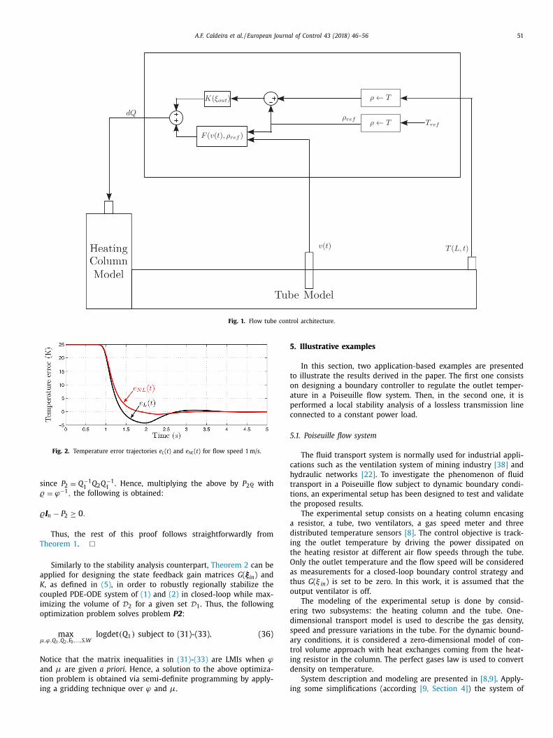

A.F. Caldeira et al. / European Journal of Control 43 (2018) 46–56 51

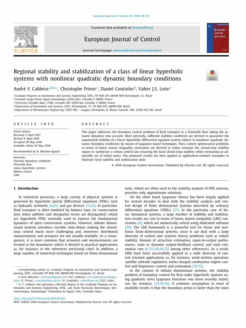
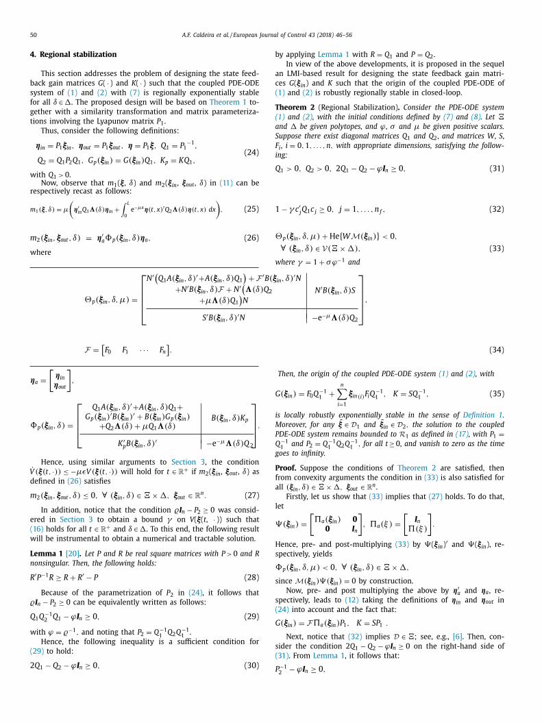
Fig. 1. Flow tube control architecture.

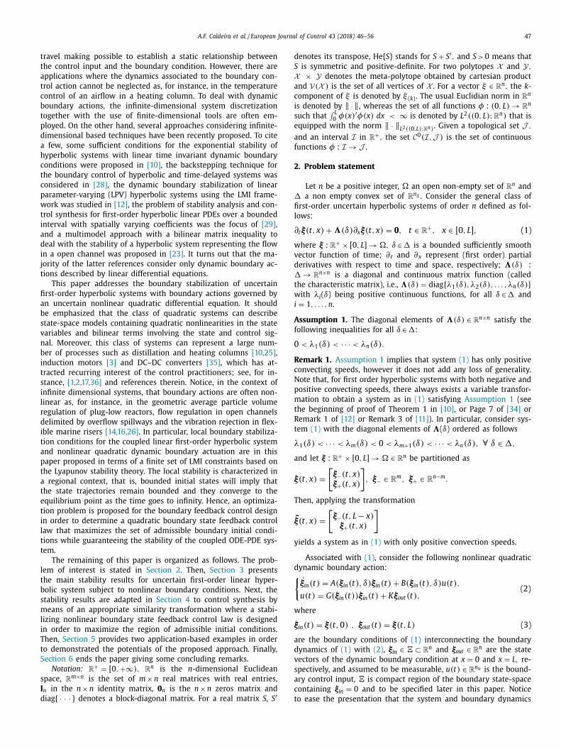
Fig. 2. Temperature error trajectories e L ( t ) and e NL ( t ) for flow speed 1 m/s.

s

�

�

T

a

K

c

i

o

μ

N

a

t

i

5

t

o

a

p

c

5

c

h

t

t

t

a

d

i

t

O

a

t

o

e

d

s

a

t

i

d

i

ince P 2 = Q

−1 1

Q 2 Q

−1 1

. Hence, multiplying the above by P 2 ϱ with

= ϕ

−1 , the following is obtained:

I n − P 2 ≥ 0 .

Thus, the rest of this proof follows straightforwardly from

heorem 1 . �

Similarly to the stability analysis counterpart, Theorem 2 can be

pplied for designing the state feedback gain matrices G ( ξin ) and

, as defined in (5) , in order to robustly regionally stabilize the

oupled PDE-ODE system of (1) and (2) in closed-loop while max-

mizing the volume of D 2 for a given set D 1 . Thus, the following

ptimization problem solves problem P2 :

max ,ϕ,Q 1 ,Q 2 ,F 0 , ... ,S,W

logdet (Q 1 ) subject to (31)-(33). (36)

otice that the matrix inequalities in (31) - (33) are LMIs when ϕnd μ are given a priori . Hence, a solution to the above optimiza-

ion problem is obtained via semi-definite programming by apply-

ng a gridding technique over ϕ and μ.

. Illustrative examples

In this section, two application-based examples are presented

o illustrate the results derived in the paper. The first one consists

n designing a boundary controller to regulate the outlet temper-

ture in a Poiseuille flow system. Then, in the second one, it is

erformed a local stability analysis of a lossless transmission line

onnected to a constant power load.

.1. Poiseuille flow system

The fluid transport system is normally used for industrial appli-

ations such as the ventilation system of mining industry [38] and

ydraulic networks [22] . To investigate the phenomenon of fluid

ransport in a Poiseuille flow subject to dynamic boundary condi-

ions, an experimental setup has been designed to test and validate

he proposed results.

The experimental setup consists on a heating column encasing

resistor, a tube, two ventilators, a gas speed meter and three

istributed temperature sensors [8] . The control objective is track-

ng the outlet temperature by driving the power dissipated on

he heating resistor at different air flow speeds through the tube.

nly the outlet temperature and the flow speed will be considered

s measurements for a closed-loop boundary control strategy and

hus G ( ξ in ) is set to be zero. In this work, it is assumed that the

utput ventilator is off.

The modeling of the experimental setup is done by consid-

ring two subsystems: the heating column and the tube. One-

imensional transport model is used to describe the gas density,

peed and pressure variations in the tube. For the dynamic bound-

ry conditions, it is considered a zero-dimensional model of con-

rol volume approach with heat exchanges coming from the heat-

ng resistor in the column. The perfect gases law is used to convert

ensity on temperature.

System description and modeling are presented in [8,9] . Apply-

ng some simplifications (according [9, Section 4] ) the system of

52 A.F. Caldeira et al. / European Journal of Control 43 (2018) 46–56

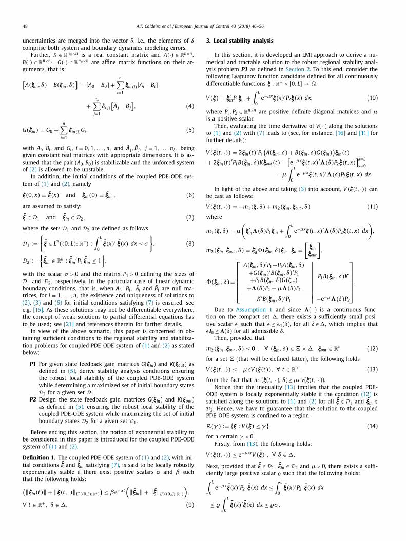
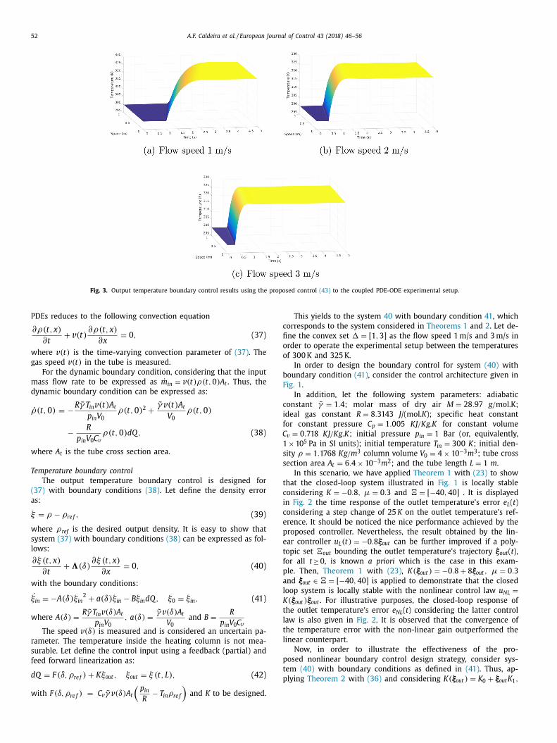
Fig. 3. Output temperature boundary control results using the proposed control (43) to the coupled PDE-ODE experimental setup.

c

fi

o

o

b

F

c

i

f

C

1

s

s

t

c

i

c

e

p

e

t

f

p

a

l

K

t

l

t

l

p

t

p

PDEs reduces to the following convection equation

∂ρ(t, x )

∂t + v (t)

∂ρ(t, x )

∂x = 0 , (37)

where v (t) is the time-varying convection parameter of (37) . The

gas speed v (t) in the tube is measured.

For the dynamic boundary condition, considering that the input

mass flow rate to be expressed as ˙ m in = v (t ) ρ(t , 0) A t . Thus, the

dynamic boundary condition can be expressed as:

˙ ρ(t, 0) = −R γ T in v (t) A t

p in V 0

ρ(t, 0) 2 +

˜ γ v (t) A t

V 0

ρ(t, 0)

− R

p in V 0 C v ρ(t, 0) dQ, (38)

where A t is the tube cross section area.

Temperature boundary control

The output temperature boundary control is designed for

(37) with boundary conditions (38) . Let define the density error

as:

ξ = ρ − ρre f , (39)

where ρref is the desired output density. It is easy to show that

system (37) with boundary conditions (38) can be expressed as fol-

lows:

∂ξ (t, x )

∂t + �(δ)

∂ξ (t, x )

∂x = 0 , (40)

with the boundary conditions:

˙ ξin = −A (δ) ξin 2 + a (δ) ξin − Bξin dQ, ξ0 = ξin , (41)

where A (δ) =

R γ T in v (δ) A t

p in V 0 , a (δ) =

˜ γ v (δ) A t

V 0 and B =

R

p in V 0 C v The speed v (δ) is measured and is considered an uncertain pa-

rameter. The temperature inside the heating column is not mea-

surable. Let define the control input using a feedback (partial) and

feed forward linearization as:

dQ = F (δ, ρre f ) + Kξout , ξout = ξ (t, L ) , (42)

with F (δ, ρre f ) = C v γ v (δ) A t

(p in R

− T in ρre f

)and K to be designed.

This yields to the system 40 with boundary condition 41 , which

orresponds to the system considered in Theorems 1 and 2 . Let de-

ne the convex set � = [1 , 3] as the flow speed 1 m/s and 3 m/s in

rder to operate the experimental setup between the temperatures

f 300 K and 325 K.

In order to design the boundary control for system (40) with

oundary condition (41) , consider the control architecture given in

ig. 1 .

In addition, let the following system parameters: adiabatic

onstant ˜ γ = 1 . 4 ; molar mass of dry air M = 28 . 97 g/ mol.K ;

deal gas constant R = 8 . 3143 J /(mol. K ); specific heat constant

or constant pressure C p = 1 . 005 K J/K g.K for constant volume

v = 0 . 718 K J/K g.K ; initial pressure p in = 1 Bar (or, equivalently,

× 10 5 Pa in SI units); initial temperature T in = 300 K; initial den-

ity ρ = 1 . 1768 Kg/m

3 column volume V 0 = 4 × 10 −3 m

3 ; tube cross

ection area A t = 6 . 4 × 10 −3 m

2 ; and the tube length L = 1 m .

In this scenario, we have applied Theorem 1 with (23) to show

hat the closed-loop system illustrated in Fig. 1 is locally stable

onsidering K = −0 . 8 , μ = 0 . 3 and = [ −40 , 40] . It is displayed

n Fig. 2 the time response of the outlet temperature’s error e L ( t )

onsidering a step change of 25 K on the outlet temperature’s ref-

rence. It should be noticed the nice performance achieved by the

roposed controller. Nevertheless, the result obtained by the lin-

ar controller u L (t) = −0 . 8 ξout can be further improved if a poly-

opic set out bounding the outlet temperature’s trajectory ξout ( t ),

or all t ≥ 0, is known a priori which is the case in this exam-

le. Then, Theorem 1 with (23) , K(ξout ) = −0 . 8 + 8 ξout , μ = 0 . 3

nd ξout ∈ = [ −40 , 40] is applied to demonstrate that the closed

oop system is locally stable with the nonlinear control law u NL =(ξout ) ξout . For illustrative purposes, the closed-loop response of

he outlet temperature’s error e NL ( t ) considering the latter control

aw is also given in Fig. 2 . It is observed that the convergence of

he temperature error with the non-linear gain outperformed the

inear counterpart.

Now, in order to illustrate the effectiveness of the pro-

osed nonlinear boundary control design strategy, consider sys-

em (40) with boundary conditions as defined in (41) . Thus, ap-

lying Theorem 2 with (36) and considering K(ξout ) = K 0 + ξout K 1 ,

A.F. Caldeira et al. / European Journal of Control 43 (2018) 46–56 53

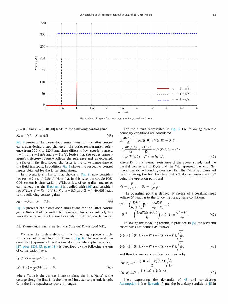
Fig. 4. Control inputs for v = 1 m / s , v = 2 m / s and v = 3 m / s .

μ

K

F

g

e

v

a

t

t

i

i

O

g

i

t

K

F

g

l

5

t

d

[

o

∂

w

v

C

b

L

w

p

t

b

b

ϕ

v

V

c

ξ

ξ

a

V

A

= 0 . 5 and = [ −40 , 40] leads to the following control gains:

0 = −0 . 9 , K 1 = 9 . 5 . (43)

ig. 3 presents the closed-loop simulations for the latter control

ains considering a step change on the outlet temperature’s refer-

nce from 300 K to 325 K and three different flow speeds (namely,

= 1 m/s , v = 2 m/s and v = 3 m/s ). Notice that the outlet temper-

ture’s trajectory robustly follows the reference and, as expected,

he faster is the flow speed, the faster is the convergence time of

he fluid transport. In addition, Fig. 4 shows the respective control

nputs obtained for the latter simulations.

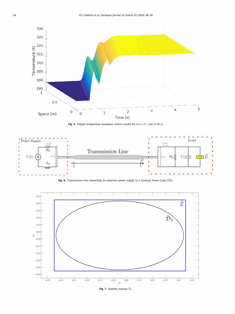
In a scenario similar to that shown in Fig. 3 , now consider-

ng v (t) = 2 + sin (12 . 56 t) . Note that in this case, the couple PDE-

DE system is time variant. Without lost of generality, and using

ain scheduling, the Theorem 2 is applied with (36) and consider-

ng K(ξout (t)) = K 0 + δ(t) ξout K 1 , μ = 0 . 5 and = [ −40 , 40] leads

o the following control gains:

0 = −0 . 6 ., K 1 = 7 . 8 . (44)

ig. 5 presents the closed-loop simulations for the latter control

ains. Notice that the outlet temperature’s trajectory robustly fol-

ows the reference with a small degradation of transient behavior.

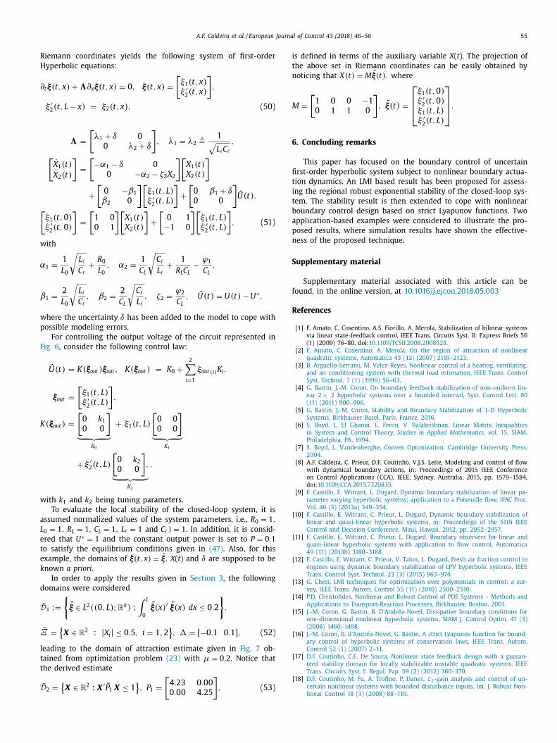
.2. Transmission line connected to a Constant Power Load (CPL)

Consider the lossless electrical line connecting a power supply

o a constant power load as shown in Fig. 6 . The electrical line

ynamics (represented by the model of the telegrapher equations

27, page 123] , [5, page 18] ) is described by the following system

f conservation laws:

∂ t I(t, x ) +

1

L � ∂ x V (t, x ) = 0 ,

t V (t, x ) +

1

C � ∂ x I(t, x ) = 0 , (45)

here I ( t , x ) is the current intensity along the line, V ( t , x ) is the

oltage along the line, L � is the line self-inductance per unit length,

� is the line capacitance per unit length.

For the circuit represented in Fig. 6 , the following dynamic

oundary conditions are considered:

0 dI(t, 0)

dt + R 0 I(t, 0) + V (t, 0) = U(t) ,

C L dV (t, L )

dt +

V (t, L )

R L

− ϕ 1 (V (t, L ) − V

∗)

+ ϕ 2 (V (t, L ) − V

∗) 2 = I(t, L ) , (46)

here R 0 is the internal resistance of the power supply, and the

arallel connection of R L , C L and the CPL represent the load. No-

ice in the above boundary dynamics that the CPL is approximated

y considering the first two terms of a Taylor expansion, with V

∗

eing the operation point and

1 =

P

(V

∗) 2 , ϕ 2 =

P

(V

∗) 3 .

The operating point is defined by means of a constant input

oltage U

∗ leading to the following steady state conditions:

∗2 −(

R L U

∗

R 0 + R L

)V

∗ +

R 0 R L P

R 0 + R L

= 0 ,

U

∗2 −(

4 R 0 P (R 0 + R L )

R L

)≥ 0 , I ∗ =

U

∗ − V

∗

R 0

. (47)

Following the modeling technique provided in [5] , the Riemann

oordinates are defined as follows:

1 (t, x ) � (V (t, x ) − V

∗) + (I(t, x ) − I ∗)

√

L �

C � ,

2 (t, x ) � (V (t, x ) − V

∗) − (I(t, x ) − I ∗)

√

L �

C � , (48)

nd thus the inverse coordinates are given by

I(t, x ) = I ∗ +

ξ1 (t, x ) − ξ2 (t, x )

2

√

C �

L � ,

(t, x ) = V

∗ +

ξ1 (t, x ) + ξ2 (t, x )

2

. (49)

Next, expressing the dynamics of 45 and considering

ssumption 1 (see Remark 1 ) and the boundary conditions 46 in

54 A.F. Caldeira et al. / European Journal of Control 43 (2018) 46–56

Fig. 5. Output temperature boundary control results for v (t) = 2 + sin (12 . 56 t) .

Fig. 6. Transmission line connecting an inductive power supply to a Constant Power Load (CPL).

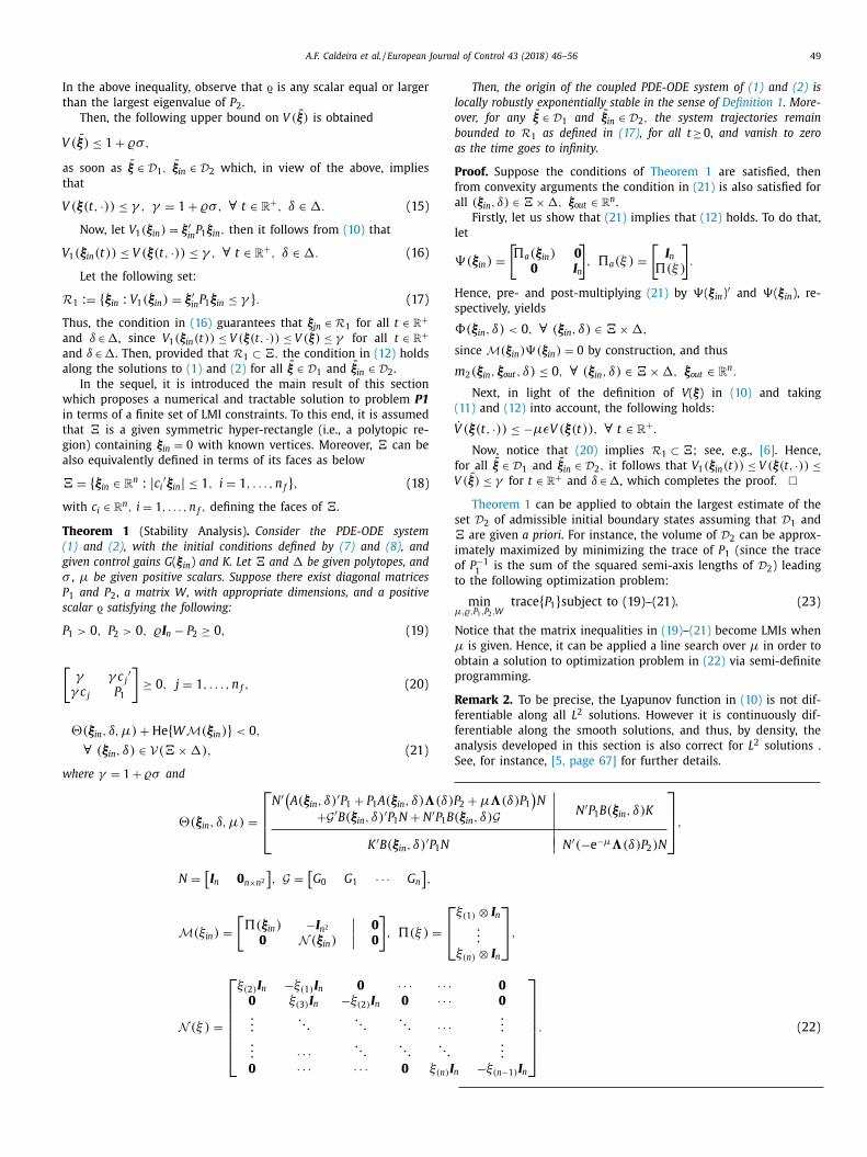
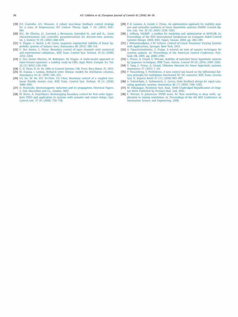
Fig. 7. Stability domain ˜ D 2 .

A.F. Caldeira et al. / European Journal of Control 43 (2018) 46–56 55

R

H

∂

[

w

α

β

w

p

F

K

w

a

L

e

t

e

k

d

D

Ξ

l

t

t

D

i

t

n

M

6

fi

t

i

t

b

a

p

n

S

f

R

iemann coordinates yields the following system of first-order

yperbolic equations:

t ξ(t, x ) + �∂ x ξ(t, x ) = 0 , ξ(t, x ) =

[ξ1 (t, x ) ξ ′

2 (t, x )

],

ξ ′ 2 (t, L − x ) = ξ2 (t, x ) , (50)

� =

[λ1 + δ 0

0 λ2 + δ

], λ1 = λ2 �

1 √

L � C � ,

[˙ X 1 (t) ˙ X 2 (t)

]=

[−α1 − δ 0

0 −α2 − ζ2 X 2

][X 1 (t) X 2 (t)

]

+

[0 −β1

β2 0

][ξ1 (t, L ) ξ ′

2 (t, L )

]+

[0 β1 + δ0 0

]ˆ U (t) .

ξ1 (t, 0) ξ ′

2 (t, 0)

]=

[1 0

0 1

][X 1 (t) X 2 (t)

]+

[0 1

−1 0

][ξ1 (t, L ) ξ ′

2 (t, L )

], (51)

ith

1 =

1

L 0

√

L �

C � +

R 0

L 0 , α2 =

1

C L

√

C �

L � +

1

R L C L − ϕ 1

C L ,

1 =

2

L 0

√

L �

C � , β2 =

2

C L

√

C �

L � , ζ2 =

ϕ 2

C L , ˆ U (t) = U(t) − U

∗,

here the uncertainty δ has been added to the model to cope with

ossible modeling errors.

For controlling the output voltage of the circuit represented in

ig. 6 , consider the following control law:

ˆ U (t) = K(ξout ) ξout , K(ξout ) = K 0 +

2 ∑

i =1

ξout (i ) K i ,

ξout =

[ξ1 (t, L ) ξ ′

2 (t, L )

],

(ξout ) =

[0 k 1 0 0

]︸ ︷︷ ︸

K 0

+ ξ1 (t, L )

[0 0

0 0

]︸ ︷︷ ︸

K 1

+ ξ ′ 2 (t, L )

[0 k 2 0 0

],

︸ ︷︷ ︸ K 2

.

ith k 1 and k 2 being tuning parameters.

To evaluate the local stability of the closed-loop system, it is

ssumed normalized values of the system parameters, i.e., R 0 = 1 ,

0 = 1 , R L = 1 , C L = 1 , L � = 1 and C � ) = 1 . In addition, it is consid-

red that U

∗ = 1 and the constant output power is set to P = 0 . 1

o satisfy the equilibrium conditions given in (47) . Also, for this

xample, the domains of ξ(t, x ) = ξ, X ( t ) and δ are supposed to be

nown a priori .

In order to apply the results given in Section 3 , the following

omains were considered

˜ 1 :=

{ξ ∈ L 2 ((0 , L ) ; R

n ) :

∫ L

0

ξ(x ) ′ ξ(x ) dx ≤ 0 . 2

},

˜ =

{X ∈ R

2 : | X i | ≤ 0 . 5 , i = 1 , 2

}, � = [ −0 . 1 0 . 1] , (52)

eading to the domain of attraction estimate given in Fig. 7 ob-

ained from optimization problem (23) with μ = 0 . 2 . Notice that

he derived estimate

˜ 2 =

{X ∈ R

2 : X

′ ˜ P 1 X ≤ 1

}, P 1 =

[4 . 23 0 . 00

0 . 00 4 . 25

], (53)

s defined in terms of the auxiliary variable X ( t ). The projection of

he above set in Riemann coordinates can be easily obtained by

oticing that X(t) = M ξ(t) , where

=

[1 0 0 −1

0 1 1 0

], ξ(t) =

⎡

⎢ ⎣

ξ1 (t, 0) ξ ′

2 (t, 0) ξ1 (t, L ) ξ ′

2 (t, L )

⎤

⎥ ⎦

.

. Concluding remarks

This paper has focused on the boundary control of uncertain

rst-order hyperbolic system subject to nonlinear boundary actua-

ion dynamics. An LMI based result has been proposed for assess-

ng the regional robust exponential stability of the closed-loop sys-

em. The stability result is then extended to cope with nonlinear

oundary control design based on strict Lyapunov functions. Two

pplication-based examples were considered to illustrate the pro-

osed results, where simulation results have shown the effective-

ess of the proposed technique.

upplementary material

Supplementary material associated with this article can be

ound, in the online version, at 10.1016/j.ejcon.2018.05.003

eferences

[1] F. Amato, C. Cosentino, A.S. Fiorillo, A. Merola, Stabilization of bilinear systems

via linear state-feedback control, IEEE Trans. Circuits Syst. II: Express Briefs 56(1) (2009) 76–80, doi: 10.1109/TCSII.2008.2008528 .

[2] F. Amato , C. Cosentino , A. Merola , On the region of attraction of nonlinearquadratic systems, Automatica 43 (12) (2007) 2119–2123 .

[3] B. Arguello-Serrano , M. Velez-Reyes , Nonlinear control of a heating, ventilating,and air conditioning system with thermal load estimation, IEEE Trans. Control

Syst. Technol. 7 (1) (1999) 56–63 .

[4] G. Bastin , J.-M. Coron , On boundary feedback stabilization of non-uniform lin-ear 2 × 2 hyperbolic systems over a bounded interval, Syst. Control Lett. 60

(11) (2011) 900–906 . [5] G. Bastin , J.-M. Coron , Stability and Boundary Stabilization of 1-D Hyperbolic

Systems, Birkhauser Basel, Paris, France, 2016 . [6] S. Boyd , L. El Ghaoui , E. Feron , V. Balakrishnan , Linear Matrix Inequalities

in System and Control Theory, Studies in Applied Mathematics , vol. 15, SIAM,

Philadelphia, PA, 1994 . [7] S. Boyd , L. Vandenberghe , Convex Optimization, Cambridge University Press,

2004 . [8] A.F. Caldeira, C. Prieur, D.F. Coutinho, V.J.S. Leite, Modeling and control of flow

with dynamical boundary actions, in: Proceedings of 2015 IEEE Conferenceon Control Applications (CCA), IEEE, Sydney, Australia, 2015, pp. 1579–1584,

doi: 10.1109/CCA.2015.7320835 .

[9] F. Castillo , E. Witrant , L. Dugard , Dynamic boundary stabilization of linear pa-rameter varying hyperbolic systems: application to a Poiseuille flow, IFAC Proc.

Vol. 46 (3) (2013a) 349–354 . [10] F. Castillo , E. Witrant , C. Prieur , L. Dugard , Dynamic boundary stabilization of

linear and quasi-linear hyperbolic systems, in: Proceedings of the 51th IEEEControl and Decision Conference, Maui, Hawaii, 2012, pp. 2952–2957 .

[11] F. Castillo , E. Witrant , C. Prieur , L. Dugard , Boundary observers for linear and

quasi-linear hyperbolic systems with application to flow control, Automatica49 (11) (2013b) 3180–3188 .

[12] F. Castillo , E. Witrant , C. Prieur , V. Talon , L. Dugard , Fresh air fraction control inengines using dynamic boundary stabilization of LPV hyperbolic systems, IEEE

Trans. Control Syst. Technol. 23 (3) (2015) 963–974 . [13] G. Chesi , LMI techniques for optimization over polynomials in control: a sur-

vey, IEEE Trans. Autom. Control 55 (11) (2010) 2500–2510 .

[14] P.D. Christofides , Nonlinear and Robust Control of PDE Systems – Methods andApplications to Transport-Reaction Processes, Birkhauser, Boston, 2001 .

[15] J.-M. Coron , G. Bastin , B. D’Andréa-Novel , Dissipative boundary conditions forone-dimensional nonlinear hyperbolic systems, SIAM J. Control Optim. 47 (3)

(2008) 1460–1498 . [16] J.-M. Coron , B. d’Andréa-Novel , G. Bastin , A strict Lyapunov function for bound-

ary control of hyperbolic systems of conservation laws, IEEE Trans. Autom.Control 52 (1) (2007) 2–11 .

[17] D.F. Coutinho , C.E. De Souza , Nonlinear state feedback design with a guaran-

teed stability domain for locally stabilizable unstable quadratic systems, IEEETrans. Circuits Syst. I: Regul. Pap. 59 (2) (2012) 360–370 .

[18] D.F. Coutinho , M. Fu , A. Trofino , P. Danes , L 2 -gain analysis and control of un-certain nonlinear systems with bounded disturbance inputs, Int. J. Robust Non-

linear Control 18 (1) (2008) 88–110 .

56 A.F. Caldeira et al. / European Journal of Control 43 (2018) 46–56

[

[

[

[19] D.F. Coutinho , A.V. Wouwer , A robust non-linear feedback control strategyfor a class of bioprocesses, IET Control Theory Appl. 7 (6) (2013) 829–

841 . [20] M.C. De Oliveira , J.C. Geromel , J. Bernussou , Extended H 2 and and H ∞ norm

characterizations and controller parametrizations for discrete-time systems,Int. J. Control 75 (9) (2002) 666–679 .

[21] A. Diagne , G. Bastin , J.-M. Coron , Lyapunov exponential stability of linear hy-perbolic systems of balance laws, Automatica 48 (2012) 109–114 .

[22] V. Dos Santos , C. Prieur , Boundary control of open channels with numerical

and experimental validations., IEEE Trans. Control Syst. Technol. 16 (6) (2008)1252–1264 .

[23] V. Dos Santos Martins , M. Rodrigues , M. Diagne , A multi-model approach toSaint-Venant equations: a stability study by LMIs, Appl. Math. Comput. Sci. Vol.

22 (3) (2012) 539–550 . [24] G.-D. Duan , H.-H. Yu , LMIs in Control Systems, CRC Press, Boca Raton, FL, 2013 .

[25] M. Espana , I. Landau , Reduced order bilinear models for distillation columns,

Automatica 14 (4) (1978) 345–355 . [26] S.S. Ge , W. He , B.V. Ee-How , Y.S. Choo , Boundary control of a coupled non-

linear flexible marine riser, IEEE Trans. Control Syst. Technol. 18 (5) (2010)1080–1091 .

[27] O. Heaviside , Electromagnetic induction and its propagation, Electrical Papers,2, 2nd, Macmillan and Co., London, 1892 .

[28] M. Krstic , A. Smyshlyaev , Backstepping boundary control for first-order hyper-

bolic PDES and application to systems with actuator and sensor delays, Syst.Control Lett. 57 (9) (2008) 750–758 .

29] P.-O. Lamare , A. Girard , C. Prieur , An optimisation approach for stability anal-ysis and controller synthesis of linear hyperbolic systems, ESAIM: Control Op-

tim. Calc. Var. 22 (4) (2016) 1236–1263 . [30] J. Lofberg , YALMIP: a toolbox for modeling and optimization in MATLAB, in:

Proceedings of the IEEE International Symposium on Computer Aided ControlSystems Design, 2004, IEEE, Taipei, Taiwan, 2004, pp. 284–289 .

[31] J. Mohammadpour , C.W. Scherer , Control of Linear Parameter Varying Systemswith Applications, Springer, New York, 2012 .

32] A. Papachristodoulou , S. Prajna , A tutorial on sum of squares techniques for

systems analysis, in: Proceedings of the American Control Conference, Port-land, OR, 2005, pp. 2686–2700 .

[33] C. Prieur , A. Girard , E. Witrant , Stability of switched linear hyperbolic systemsby Lyapunov techniques, IEEE Trans. Autom. Control 59 (8) (2014) 2196–2202 .

[34] Y. Tang , C. Prieur , A. Girard , Tikhonov theorem for linear hyperbolic systems,Automatica 57 (2015) 1–10 .

[35] P. Thounthong , S. Pierfederici , A new control law based on the differential flat-

ness principle for multiphase interleaved DC–DC converter, IEEE Trans. CircuitsSyst. II: Express Briefs 57 (11) (2010) 903–907 .

36] G. Valmórbida , S. Tarbouriech , G. Garcia , State feedback design for input-satu-rating quadratic systems, Automatica 46 (7) (2010) 1196–1202 .

[37] M. Vidyasagar , Nonlinear Syst. Anal., SIAM Unabridged Republication of Origi-nal Work Published by Prentice-Hall, 2nd, 2002 .

[38] E. Witrant , K. Johansson , HYNX team , Air flow modelling in deep wells: ap-

plication to mining ventilation, in: Proceedings of the 4th IEEE Conference onAutomation Science and Engineering, 2008 .