estimation of hydraulic conductivity from grain size...
TRANSCRIPT

Estimation of Hydraulic Conductivity
from Grain Size Analyses
A comparative study of different sampling and calculation
methods focusing on Västlänken
Master of Science Thesis in the Master’s Programme Geo and Water Engineering
ANDREA SVENSSON
Department of Civil and Environmental Engineering
Division of GeoEngineering
Engineering Geology Research Group
CHALMERS UNIVERSITY OF TECHNOLOGY
Göteborg, Sweden 2014
Master’s Thesis 2014:1


MASTER’S THESIS 2014:1
Estimation of Hydraulic Conductivity
from Grain Size Analyses
A comparative study of different sampling and calculation methods focusing on
Västlänken
Master of Science Thesis in the Master’s Programme Geo and Water Engineering
Department of Civil and Environmental Engineering
Division of GeoEngineering
Engineering Geology Research Group
CHALMERS UNIVERSITY OF TECHNOLOGY
Göteborg, Sweden 2014
Estimation of Hydraulic Conductivity from Grain Size Analyses
A comparative study of different sampling and calculation methods focusing on
Västlänken Master of Science Thesis in the Master’s Programme Geo and Water Engineering
ANDREA SVENSSON
Examensarbete / Institutionen för bygg- och miljöteknik,
Chalmers tekniska högskola 2014:
Department of Civil and Environmental Engineering
Division of GeoEngineering
Engineering Geology Research Group
Chalmers University of Technology
SE-412 96 Göteborg
Sweden
Telephone: + 46 (0)31-772 1000
Cover:
Grain size curve from borehole OC4008-1 at Skansen Lejonet. The results are
interpreted in chapter 8.
Department of Civil and Environmental Engineering
Göteborg, Sweden 2014

I
Estimation of Hydraulic Conductivity from Grain Size Analyses
A comparative study of different sampling and calculation methods focusing on
Västlänken Master of Science Thesis in the Master’s Programme Geo and Water Engineering
ANDREA SVENSSON
Department of Civil and Environmental Engineering
Division of GeoEngineering
Engineering Geology Research Group
Chalmers University of Technology
ABSTRACT
The purpose of this thesis is to evaluate different methods to calculate hydraulic
conductivity, as well as to compare the methods to obtain soil samples used in the
project Västlänken, with sampling methods used in this thesis. Soil samples from two
locations, Skansen Lejonet and Korsvägen, were taken. Laboratory work such as grain
size analyses and different porosity measurements were used on these samples. By
using a version of the Kozeny-Carman method to calculate hydraulic conductivity, the
results were compared to the most common methods, Hazen and Gustafson. The
values from the previous sampling in the project were also used to calculate hydraulic
conductivity with Kozeny-Carman. The three methods were compared to each other
and the results from the previous soil sampling were compared with the results from
the current sampling performed in this thesis. The results from grain size analyses
were also compared with slug tests and pumping tests performed in the project
Västlänken. The results showed that the Kozeny-Carman equation generally gives a
lower conductivity than the Hazen and Gustafson equation, but may be more in line
with the results from the hydraulic tests. The results also showed that there were very
small differences between the more limited sampling method used previously and the
sampling methods used in this thesis. The conclusion drawn from these results was
that for test sites with fairly homogenous soil like Korsvägen and especially Skansen
Lejonet the limited sampling method is accurate enough. The more elaborate
laboratory work needed to use the Kozeny-Carman method may discourage the use of
this method. However, if some work were performed on classifying the degree of
compaction of a soil sample easily, the Kozeny-Carman method would be easier to
use. The conclusion is that the Kozeny-Carman method could be useful to evaluate
the hydraulic conductivity from grain size analyses with more accuracy.
KEY WORDS: hydraulic conductivity, grain size analysis, Kozeny-Carman equation,
soil sampling, porosity, Västlänken.

II

CHALMERS, Civil and Environmental Engineering, Master’s Thesis 2014:1 III
Contents
ABSTRACT ................................................................................................................... I
CONTENTS ................................................................................................................. III
HANDLEDARENS FÖRORD .................................................................................. VII
PREFACE ................................................................................................................. VIII
NOTATIONS .............................................................................................................. IX
1 INTRODUCTION ................................................................................................. 1
1.1 Background .............................................................................................................. 1
1.2 Aim and objections .................................................................................................. 2
1.3 Delimitations ............................................................................................................ 2
2 HYDROGEOLOGICAL CONCEPTS .................................................................. 3
2.1 Darcy’s law .............................................................................................................. 3
2.2 Soil properties .......................................................................................................... 3
2.2.1 Grain size ............................................................................................................. 3
2.2.2 Porosity ................................................................................................................ 4
2.2.3 Degree of compaction .......................................................................................... 4
2.2.4 Grain shape .......................................................................................................... 4
2.3 Hydraulic conductivity ............................................................................................. 4
3 LITERATURE REVIEW ...................................................................................... 5
3.1 Comparison between field methods and grain size analyses ................................... 5
3.2 Evaluation of the Kozeny-Carman equation ............................................................ 6
3.3 Comparison between laboratory methods and grain size analyses .......................... 7
3.4 Porosity .................................................................................................................... 8
4 HYDROGEOLOGICAL ENVIRONMENT ....................................................... 10
4.1 Skansen Lejonet ..................................................................................................... 11
4.2 Korsvägen .............................................................................................................. 11
5 METHODS FOR MEASURING HYDRAULIC CONDUCTIVITY ................. 15
5.1 Indirect methods ..................................................................................................... 15
5.1.1 Hazen ................................................................................................................. 15
5.1.2 Gustafson ........................................................................................................... 15
5.1.3 Kozeny-Carman ................................................................................................. 16
5.2 Hydraulic tests........................................................................................................ 19
5.2.1 Pumping test ...................................................................................................... 19
5.2.2 Slug test ............................................................................................................. 19
5.3 Laboratory methods ............................................................................................... 19

IV CHALMERS, Civil and Environmental Engineering, Master’s Thesis 2014:1
5.4 Porosity .................................................................................................................. 20
6 METHODOLOGY LABORATORY WORK ..................................................... 22
6.1 Grain size analysis ................................................................................................. 22
6.2 Permeameter test .................................................................................................... 23
6.3 Compact density ..................................................................................................... 23
6.4 Bulk density ........................................................................................................... 24
6.5 Porosity .................................................................................................................. 24
6.5.1 Porosity measurements on Skansen Lejonet samples ........................................ 25
6.5.2 Porosity measurements on Korsvägen samples ................................................. 25
7 EXECUTION AND OBSERVATIONS.............................................................. 27
7.1 Soil sampling ......................................................................................................... 27
7.1.1 Skansen Lejonet ................................................................................................. 27
7.1.2 Korsvägen .......................................................................................................... 29
7.2 Previous sampling .................................................................................................. 30
7.2.1 Soil sampling for grain size analyses ................................................................. 30
7.2.2 Slug tests ............................................................................................................ 31
7.2.3 Pumping tests ..................................................................................................... 31
7.3 Laboratory work ..................................................................................................... 31
7.4 Calculations of hydraulic conductivity .................................................................. 32
8 RESULTS ............................................................................................................ 33
8.1 Porosity .................................................................................................................. 33
8.2 Hydraulic conductivity ........................................................................................... 35
8.3 Previous sampling – grain size analysis ................................................................. 38
8.4 Hydraulic tests........................................................................................................ 42
8.4.1 Slug tests ............................................................................................................ 42
8.4.2 Pumping tests ..................................................................................................... 43
8.5 Statistical analysis .................................................................................................. 44
9 EVALUATION OF RESULTS ........................................................................... 45
9.1 The effect of porosity on Kozeny-Carman results ................................................. 46
9.2 Permeameter test .................................................................................................... 47
9.3 Comparison between previous and current sampling at Skansen Lejonet ............. 48
9.4 Comparison between previous and current sampling at Korsvägen ...................... 50
9.5 Comparison between grain size analysis and hydraulic tests at Skansen Lejonet . 51
9.6 Comparison between grain size analysis and hydraulic tests at Korsvägen........... 52
9.7 Uncertainties .......................................................................................................... 52
9.8 Consequences of selecting method ........................................................................ 53

CHALMERS, Civil and Environmental Engineering, Master’s Thesis 2014:1 V
10 CONCLUSIONS.................................................................................................. 55
11 BIBLIOGRAPHY ................................................................................................ 57
APPENDIX 1. SKANSEN LEJONET ........................................................................ 60
APPENDIX 2. KORSVÄGEN .................................................................................... 69
APPENDIX 3. VARIATION OF HYDRAULIC CONDUCTIVITY BASED ON
DEGREE OF COMPACTION .................................................................................... 76
APPENDIX 4. GRAPH OF DIFFERENT POROSITIES BASED ON DEGREE OF
COMPACTION AND EXPERIMENTAL POROSITY ............................................. 78
APPENDIX 5. ANOVA SINGLE FACTOR ANALYSIS ......................................... 79

VI CHALMERS, Civil and Environmental Engineering, Master’s Thesis 2014:1

CHALMERS, Civil and Environmental Engineering, Master’s Thesis 2014:1 VII
Handledarens förord
Syftet med föreliggande examensarbete har varit att i projektet Västlänken belysa
skillnader i resultat vid användning av olika metoder för beräkning av hydraulisk
konduktivitet från siktanalyser. Även provtagningsmetodikens betydelse för
jordprovets sammansättning har varit av intresse.
I projekt Västlänken har jordlagrens genomsläpplighet till viss del karaktäriserats
genom siktanalyser av jordprov. Grundvattenrör med 8 mm hål har drivits ned till
friktionsjorden, jordprov har tagits på material som spolats upp och dessa har sedan
siktats. I grundvattenrören har även slugtester utförts och i två fall har
provpumpningar i filterbrunnar genomförts.
I flertalet fall har resultat från siktanalyser och slugtester haft dålig överensstämmelse,
då det trängt in fint jordmaterial i grundvattenrören, vilket innebär att rören har satt
igen. Vid tolkningen av jordlagrens genomsläpplighet har siktanalyserna bedömts
som mer trovärdiga. Beräkning av hydraulisk konduktivitet har utförts på tidigare
siktade prover och prov tagna under examensarbetet. Beräkningarna har utförts med
ekvationer av Kozeny-Carman (vidareutvecklad av Bengt Åhlén), Hazen och
Gustafson.
Två kompletterande jordprovtagningar har utförts med ambition att få med såväl
fraktioner grövre än 8 mm som de finaste fraktionerna. Resultaten har jämförts med
de tidigare provtagningarna.
Trafikverket har bistått med finansiering av jordprovtagning och tillhandahållit data.
Trafikverkets ansvarige hydrogeolog i projekt Västlänken Tekn Lic Bengt Åhlén har
bistått med expertkunskap och resultat från sin forskning gällande beräkningar av
hydraulisk konduktivitet från siktanalyser samt deltagit i att formulerat
frågeställningarna. SGUs geolog Docent Tore Påsse har ställt upp med tid och
beräkningsunderlag för hur siktkurvor kan kompenseras för bortfall av grövre
fraktioner i provtagningen.
Andrea Svensson har självständigt och entusiastiskt genomfört examensarbetet.
Arbetet för Andrea har inneburit många utmaningar med att söka relevant information
och lösningar för att ta reda på efterfrågade parametrar som legat till grund för
beräkningarna, vilket hon har genomfört på ett beundransvärt sätt.
Extern handledare
Bergab – Berggeologiska Undersökningar AB
Annika Nilsson

VIII CHALMERS, Civil and Environmental Engineering, Master’s Thesis 2014:1
Preface
This master thesis has been carried out at the department of Civil and Environmental
Engineering, Division of GeoEngineering at Chalmers University of Technology. It
was initiated by Bengt Åhlen at the Swedish Transport Administration and Annika
Nilsson at Bergab – Berggeologiska Undersökningar AB. Supervisors have been
Annika Nilsson at Bergab and Lars Rosén at Chalmers. Examiner has been Lars
Rosén at Chalmers. The Swedish Transport Administration have made the sampling
possible.
I would especially like to thank my supervisor Annika Nilsson for guidance and
support during the entity of this project. I also want to thank Lars Rosén for his
comments and help. Further I would like to thank Bengt Åhlén who has been a source
of expert knowledge in this thesis, Peter Hedborg and Mona Pålsson in the
geotechnical and environmental chemistry laboratory at Chalmers for help with the
laboratory investigations, and Tore Påsse at SGU for his time and guidance. I also
want to express my appreciation to everyone at Bergab for their interest and
encouragement.
Finally, my thanks goes to my family, especially Robert Lanzky, for their endless
support, encouragement and constructive criticism.
Gothenburg, March 2014
Andrea Svensson

CHALMERS, Civil and Environmental Engineering, Master’s Thesis 2014:1 IX
Notations
Roman upper case letters
A = Area [cm2]
A0= See Åberg, 1993
AC=Cross sectional area of channel [m2]
As = Cross sectional area of sample [m2]
B0= See Åberg, 1993
CH = Empirical constant [-]
Cu = Coefficient of uniformity [-]
d= Degree of compaction [-]
de= Effective grain size diameter [mm]
dh/dl = Hydraulic gradient [-]
d10 = The particle size for which 10% of the material is finer [mm]
d20 = The particle size for which 20% of the material is finer [mm]
d50 = The particle size for which 50% of the material is finer [mm]
d60 = The particle size for which 60% of the material is finer [mm]
E = See Andersson et. al 1984
e = Euler’s number, mathematical constant [-]
E(CU) = See Andersson et. al 1984
G(CU) = See Andersson et. al 1984
h = Height of water pillar [cm]
K = Hydraulic conductivity [m/s]
k0 = Constant [-]
L = Length of test piece [m]
L1,L2,L3=Different levels of the test piece L [m]
l = Length of sample [cm]
Le = Average length of capillaries [m]
m = hydraulic radius [m]
ms = Mass of soil [g]
msoil = Weight of soil sample [g]
mw = Mass of water [g]
m1 = Weight of empty container [g]
m2 = Weight of container and mineral turpentine [g]
m3 = Weight of soil sample [g]

X CHALMERS, Civil and Environmental Engineering, Master’s Thesis 2014:1
m4 = Weight of soil sample and mineral turpentine [g]
m5 = Mass of cylinder [g]
m6 = Mass of water up to mark and cylinder [g]
m7 = Mass of soil up to mark and cylinder [g]
m8 = Mass of water and soil up to mark and cylinder [g]
n = Porosity [-]
P=Wetted perimeter [m2]
Q = Flow [m3/s]
R = Coefficient of roughness [-]
Re = Effective radial distance over which y is dissipated [m]
rw = Radius of influence [m]
S=Particle surface for unit volume of the porous media [-]
S0 = Specific grain surface of solids [-]
T = Transmissivity [m2/s]
t = Time for water flowing through the sample [s]
V = Volume of water flowing through the sample [cm3]
Vsoil = Volume of soil sample [cm3]
Vpy = Volume of pycnometer [cm3]
Vw = Volume of water [cm3]
w = Water content [%]
y= Vertical difference between water level inside well and static water Table
outside well
[m]
Greek letters
γ =Specific weight [N/m3]
ε = Void ratio [-]
μ = Viscosity [(Ns)/m2]
μG =Geometric mean [mm]
ρ = Bulk density of soil sample [g/cm3]
ρs = Compact density of soil sample [g/cm3]
ρ1 = Density of mineral turpentine [g/cm3]
σ =Geometric standard deviation [mm]
τ = Ratio of kinematic viscosity at 10°C and ground water temperature [-]

CHALMERS, Civil and Environmental Engineering, Master’s Thesis 2014:1 XI


CHALMERS, Civil and Environmental Engineering, Master’s Thesis 2014:1 1
1 Introduction
When conducting a hydrogeological study, hydraulic conductivity is one of the most
important parameters, but also a parameter that is difficult to determine. This master
thesis will study hydraulic conductivity in soils, focusing on the project Västlänken in
Gothenburg. Samples have been taken from two different locations along the
Västlänken stretch, Korsvägen and Skansen Lejonet. These samples was tested in a
laboratory and several different methods to calculate hydraulic conductivity was used
and compared to each other and to the results from previous sampling in the project.
1.1 Background
The project Västlänken is a railway tunnel through central Gothenburg, see Figure 1.
In addition to the existing station Centralstationen, two stations will be constructed at
Korsvägen and Haga. Due to the sensitive urban environment there are many
challenges that have to be solved in this project. As there are a lot of buildings in the
vicinity and the ground has been drained previously, the ground is sensitive to
settlements. Due to this, the hydrogeological properties, such as the hydraulic
conductivity, are important to know. There can be different consequences both if the
hydraulic conductivity is overestimated and if it is underestimated. In questions of
leakage into for example a tunnel, an overestimation of the hydraulic conductivity is
conservative, but in questions of infiltration the opposite is true. Misjudgements that
lead to settlements or other damages can have great financial consequences and also
legal repercussions.
Figure 1 The stretch of the railway tunnel through central Gothenburg (Trafikverket, 2013)

2 CHALMERS, Civil and Environmental Engineering, Master’s Thesis 2014:1
Several different methods exist to estimate a hydraulic conductivity, both from
laboratory work, indirect methods such as grain size analyses and from hydraulic
tests. Besides the grain size, other parameters such as degree of compaction, porosity
and shape of the grains all have an effect on the hydraulic conductivity. It is also
important to be aware of and understand the hydrogeological environment, for
example since the sedimentological environment determines the degree of
compaction.
As changes in the groundwater Table, depending on the hydraulic conductivity, can
affect the area in many ways, knowing if the estimated value is accurate is important.
More theoretically, investigating how different soil parameters affect the hydraulic
conductivity and what results different methods provide, can give an increased
understanding of hydraulic conductivity and improve the accuracy when estimating it.
In the Västlänken project geological investigations have been made throughout the
route. When studying the hydrogeology in the area, soil samples have been taken
from boreholes and grain size analyses have been made on these samples to determine
the hydraulic conductivity. Some hydraulic tests have also been made, such as slug
tests and test pumping.
1.2 Aim and objections
The overall aim of this master thesis is to compare different methods to estimate
hydraulic conductivity through grain size analyses and correlate it with results from
hydraulic tests. The test methods to achieve a soil sample have different uncertainties
that all affect the estimations of hydraulic conductivity. In the scope of this master
thesis investigations of soil samples will be conducted to determine the hydraulic
conductivity. A comparison of different sampling methods will be made.
The specific objective of this thesis focus on Västlänken, and will evaluate if the test
methods used for sampling gives accurate results, or if more undisturbed sampling
methods provide more accurate results. Conclusions will also be drawn on the
applicability on several methods used to calculate hydraulic conductivity in this
thesis.
1.3 Delimitations
The laboratory work on the soil samples have focused on grain size analysis and
porosity. Grain shape, which also affect the hydraulic conductivity and might be
interesting to look at in another study, have not be studied in this thesis. Another
important factor is degree of compaction, but due to the limited amount of sample
material this has not been part of the laboratory work to desired extent. As the thesis
focuses on the project Västlänken, the soil samples is limited to samples from the area
Korsvägen and Skansen Lejonet in Gothenburg.

CHALMERS, Civil and Environmental Engineering, Master’s Thesis 2014:1 3
2 Hydrogeological concepts
To understand the principles of hydraulic conductivity, some basic concepts are
presented in this section. The flow of groundwater in a soil is determined by the
material properties of the soil, as well as basic physical laws.
2.1 Darcy’s law
The flow of groundwater depends on the hydraulic gradient and the hydraulic
conductivity (Knutsson & Morfeldt, 2002). The flow of a fluid in porous medium can
be described by Darcy’s law, see equation 2.1.
𝑄 = −𝐾𝐴
𝑑ℎ
𝑑𝑙 2.1.
Q = Flow [m3/s]
K = Hydraulic conductivity [m/s]
A = Area [m2]
dh/dl = Hydraulic gradient [-]
The difference in height and length is represented by the hydraulic gradient, and is the
reason for the negative sign as the water flows from higher to lower level. When
describing ground water flow, Darcy’s law is altered to describe all three dimensions.
Often, this is simplified to describe 2-dimensional flow. Depending on type of
aquifer, different partial differential equations are used to describe the flow, like the
Laplace equation. To solve these equations analytically, idealized cases are used and
the boundary conditions of the aquifer must be known. By using a conceptual model
of a ground water system, reality can be translated and simplified into a manageable
model.
2.2 Soil properties
The hydraulic conductivity varies in different soils. A sorted soil like an esker deposit
has a high conductivity, and is therefore often used for ground water extraction. In
Sweden, the most common soil type is glacial till, which is an unsorted soil (Knutsson
& Morfeldt, 2002). It is often difficult to determine hydraulic conductivity in an
unsorted soil due to the great variation in the composition of the soil. In a glacial till,
the grain size varies a lot as well as the degree of compaction. Unsorted soils often
show a high degree of anisotropy; the hydraulic conductivity depends on the direction
of measurement. This means that the hydraulic conductivity is different in a
horizontal orientation than in a vertical direction.
2.2.1 Grain size
The grain size distribution of a soil is one of the soil mechanic properties that affect
the hydrogeological conductivity. A sorted soil with larger grains has a high hydraulic
conductivity. If a sediment contains a mixture of grain sizes, a more multi-graded soil,
the porosity will be lowered, and thus the hydraulic conductivity (Fetter, 2001). This
is because the void between the larger grains is filled up with smaller grains.

4 CHALMERS, Civil and Environmental Engineering, Master’s Thesis 2014:1
2.2.2 Porosity
Porosity is defined as the relationship between the pore volume and the total volume,
i.e. the air voids in a soil (Larsson, 2008). The porosity can be calculated indirectly by
knowing the compact density of the soil and the dry density (Knutsson & Morfeldt,
2002). When calculating hydraulic conductivity, the interesting parameter is the
effective porosity, the volume of the pores where water can move freely, as opposed
to total porosity where closed pores also are calculated.
2.2.3 Degree of compaction
The porosity depends on the degree of compaction. The dry density of a soil
compared to the maximum dry density where the material has been compacted in a
laboratory is called the degree of compaction (Fagerström, 1973). Different degrees of
compaction give different optimal water content, where the bulk density is the
highest.
2.2.4 Grain shape
Hydraulic conductivity is also determined by the systems formed by the voids
between the grains (Fetter, 2001). Well-rounded grains may be almost perfect
spheres, but grains can also be very irregular. Different grain shapes create different
ways for the water to move through, see Figure 2. In theory, grains are usually
assumed to be spherical, which can become a source of error in estimations of
hydraulic conductivity if the grains are very angular.
Figure 2 Different grain shape makes the water travel in different paths (Fagerström & Wiesel,
1972)(modified)
2.3 Hydraulic conductivity
In the field of hydrogeology, it is important to know how easy water (or other fluids)
can move through a porous media, i.e. hydraulic conductivity. Hydraulic conductivity
describes a material’s ability to let water through. This is defined in terms of volume
per area and time, m3/m2/s = m/s, which should not be confused with meter per
second as a velocity (Fetter, 2001). This parameter is not always easily measured, but
often has to be predicted by using basic information and translating it into estimates
of hydraulic conductivity. Hydraulic conductivity can be estimated by using methods
based on grain size analysis or determined by the use of experimental in situ- or
laboratory methods. The grain-size methods use coefficients that are estimated from
empirical data, as well as some kind of representative value of the grain size. The
experimental methods measure the flow in a soil material and calculate the hydraulic
conductivity or transmissivity from the flow in different ways. The different methods
will be described more in detail further on.

CHALMERS, Civil and Environmental Engineering, Master’s Thesis 2014:1 5
3 Literature review
It is common to determinate hydraulic conductivity from grain size analyses as the
methods are cheap and easy to use. As there are simplifications in these methods,
there are some uncertainties in how these methods reflect the reality.
Many authors have studied the hydraulic conductivity regarding what method are
most accurate, comparing methods based on grain-size distributions to hydraulic tests,
evolving the methods in different ways to make them more accurate or compare the
methods to each other. This literature review is a selection of some of the studies that
has been made. .
3.1 Comparison between field methods and grain size
analyses
Vienken and Dietrich (2011) compared many different methods to evaluate hydraulic
conductivity from grain size analyses with slug tests. They used sonic sampling to
collect core samples for their laboratory work, to try to avoid the disturbances that
typically occur during sampling. The sampling site was chosen for its high degree of
heterogeneity and broad sedimentological spectrum of deposits and 108 samples were
chosen. Grain size analyses were performed on the samples and factors like porosity
and shape factor used in the Kozeny-Carman equation were estimated with formulas
derived from the grain size analyses. When comparing the different methods to each
other, several of the methods showed a high correlation but some methods such as the
modified Kozeny-Carman equation, Kozeny-Köhler, see equation 3.1, showed larger
differences.
𝐾 =𝜏
𝑅∙ 405 ∙
𝜀3
(1 + 𝜀)∙ 𝑑𝑒
2 3.1.
K = Hydraulic conductivity [m/s]
τ = Ratio of kinematic viscosity at 10°C and ground water temperature [-]
R = Coefficient of roughness [-]
ε = Void ratio [-]
de = Effective grain size diameter [mm]
The slug test measures primarily horizontal conductivity, which in this site is
primarily greater than the vertical conductivity. This is in contrast to the hydraulic
conductivity from grain size data that measure a sort of cross between the horizontal
and vertical conductivity, as the sieving process destroys the natural sediments. When
comparing the hydraulic conductivity from grain size methods to the hydraulic
conductivity from slug tests the correlation was rather high for most methods,
however the grain size conductivity was usually smaller than the slug test
conductivity. The methods that used porosity, like Kozeny-Köhler, showed less
correlation to slug tests than the other methods. The authors concluded that the
method applied to estimate porosity has a great impact on the result and should be
chosen carefully.

6 CHALMERS, Civil and Environmental Engineering, Master’s Thesis 2014:1
Cheong et al. (2008) performed another study were hydraulic conductivity determined
from grain size analyses were compared to hydraulic conductivity determined from
slug test, pumping test and numeric modelling respectively. The numerical modelling
was performed in MODFLOW to take into account heterogeneous, anisotropic
aquifers and irregular boundary conditions. The authors argued that because of this,
the values obtained by numerical modelling are more reasonable than the values from
grain size analyses or aquifer tests. For the grain size analyses, 184 samples from
eight boreholes were used. The porosity measurements were calculated by comparing
the volume of dried samples to saturated samples. The friction soils in the studied area
consist of upper fine, medium and lower fine sands, and a highly conductive
sand/gravel layer. The sand/gravel layer is the main aquifer.
The results of the study showed varying results depending on the method and the
studied layer. The horizontal hydraulic conductivity estimated from numerical
modelling corresponded well to hydraulic conductivity estimated from grain size
analysis when comparing the sand/gravel layers but not for the fine or medium sand
layers. The hydraulic conductivity from pumping test was slightly smaller than the
hydraulic conductivity from grain size analysis when comparing the medium sands
and sand/gravel layers, but higher for the fine sand layers. The hydraulic conductivity
from slug tests was smaller than both the hydraulic conductivity from pumping tests
as well as grain size analyses.
3.2 Evaluation of the Kozeny-Carman equation
When using the Kozeny-Carman equation, more care must be taken to receive
accurate results due to the fact that several parameters are included in the equation
and thus more uncertainties than for example Gustafson’s equation. Chapuis and
Aubertin (2003) reviewed many test results from several studies and compared
measured hydraulic conductivity to predicted hydraulic conductivity. They used
permeameter tests to measure the hydraulic conductivity and the Kozeny-Carman
equation to predict it. The specific surface is one important parameter in the Kozeny-
Carman equation, which can be difficult to estimate. The authors estimated the
specific surface from the gradation curve, by using an equation where the specific
surface is calculated by using the percentage of each grain size together with the
specific gravity of the material.
The authors found that when using the Kozeny-Carman equation correctly, especially
with regards to the specific surface factor, the predictions corresponds fairly well to
measured hydraulic conductivity. It is also important to take care when performing
the permeameter test, for example as the material has to be fully saturated to reach a
steady-state condition. Besides these practical reasons, there are also theoretical
reasons when the results from the Kozeny-Carman equation show discrepancies, for
example when the soil is anisotropic. They conclude that the Kozeny-Carman
equation is a good predictive tool for any natural homogenous soil, and specialists in
geotechnics and hydrogeology should use it more systematically.

CHALMERS, Civil and Environmental Engineering, Master’s Thesis 2014:1 7
3.3 Comparison between laboratory methods and grain size
analyses
Eggleston and Rojstaczer (2001) compared in-situ measurements of hydraulic
conductivity by the use of an air permeameter, to hydraulic conductivity calculated
with the Hazen equation. In theory, hydraulic conductivity should increase with
effective grain size and decrease with grain size variability. The authors have found
this to be generally true but point out that the hydraulic conductivity is sensitive to
other parameters such as sediment stratification, low weight percentage fines and
cementation. The conclusions drawn in the article is that firstly, the hydraulic
conductivity values achieved by the Hazen equation are much too high. The authors
believe that the Hazen coefficients in order for the equation to be more accurate
should be empirically fitted. Secondly, the values have less variability than they
should, particularly if lower hydraulic conductivity values are not sampled. This
means that in an aquifer where there is strong fine scale variability, as much as
several hundred measurements may be needed to adequately characterize the aquifer.
Another article (Carrier, 2003) also finds uncertainties in the Hazen coefficient. The
author argues that the coefficient varies from 1 up to 1000 in various geotechnical
textbooks, which results in a large spread of the hydraulic conductivity when using
Hazen. The author theoretically compares the Hazen equation to the Kozeny-Carman
equation, and argues that the difficulties with the Kozeny-Carman equation, namely to
determine the specific surface, is easier today when the use of computers is
widespread. The conclusion is that the Kozeny-Carman equation is superior to the
Hazen equation in terms of accuracy, and should be preferred.
Mbonimpa et al (2002) have also argued that the Hazen coefficient has limitations,
and have proposed a function for determining this coefficient by using an extension of
the Kozeny-Carman function. The aim of the study was to use pedotransfer functions,
i.e. functions that translate readily available data into estimates of soil properties that
are more difficult to determine, such as grain size and density, to determine hydraulic
conductivity. The authors define the surface area by using the effective diameter and
uniformity coefficient. The tests described in the article were conducted on
reconstituted samples and used permeameters and triaxial cells to measure hydraulic
conductivity experimentally. Results from using the function with data from several
different studies have shown good agreement for a wide spectrum of materials. The
conclusion is that the function may be used to obtain useful information about the
hydraulic conductivity during the phase of preliminary analyses and also to check if a
questionable test result is reasonable.
Boadu (2000) studied hydraulic conductivity and developed new models from grain
size distribution based on multivariate regression analysis. Both the Hazen and
Kozeny-Carman equation uses representative grain size diameters. The author argues
that using the geometric mean of a grain size distribution does not work for all types
of soil. If the soil has a significant fine content, the harmonic mean provides a more
accurate hydraulic conductivity than the geometric mean. As the harmonic mean puts
greater weight on smaller grain sizes and the geometric mean puts greater weight on
larger sizes, it is important to choose the right representative grain size diameter. This
also depends on the state of sorting and packing. In this study, soil samples were
compacted similar to the standard Proctor compaction tests, and measurements of the
hydraulic conductivity were made with both the falling head method and the constant

8 CHALMERS, Civil and Environmental Engineering, Master’s Thesis 2014:1
head method. Sieve analyses were also made to provide grain size distributions. By
using fractal analysis of the grain size distribution, a model to determine hydraulic
conductivity based on fractal dimension, entropy, fractional porosity, percent of fine
material and bulk density were developed. The author argues that Hazen and Kozeny-
Carman were developed based on representative grain sizes of soil samples, and gives
erroneous results when the grain size distribution is different, while this model
compensate for these differences.
These studies all deal with methods of measuring hydraulic conductivity, although
from different premises. Despite the fact that some authors draw the conclusion that
using Kozeny-Carman equation is the best way to calculate hydraulic conductivity
from grain size distributions, others believe that the multitude of parameters makes it
more difficult to use and creates more uncertainties. The use of the Hazen equation,
and in Sweden the Gustafson equation, is widespread. Their simplicity makes it
unlikely that these methods will be abandoned, unless an application for the Kozeny-
Carman equation is developed that makes it easier to use.
3.4 Porosity
Frings et al (2011) studied the accuracy of porosity predictors for fluvial sand-gravel
deposits. They looked at several ways to measure porosity based on different
parameters such as effective grain size, standard deviation, deviation of the grain size
distribution from a type curve and theoretical predictors that take mixing processes
into account and calculate porosity computationally. They used laboratory methods
and in-situ experiments to calculate the porosity and compared this to different
methods based on the parameters mentioned above. The uncertainty of the laboratory
methods could lead to an overestimation of the porosity, mainly due to disturbance of
the packing near the container walls, but the authors believed that this overestimation
was probably small. In addition to the experimentally obtained results, the authors
also used two porosity data sets from literature to compare to.
The results showed that empirical predictors based on the relation between median
grain size and the porosity did not correspond very well to the laboratory results. In
part, this is because the finer sediments of a grain size distribution often represents a
small percentage of the entire distribution, and does not affect the median grain size a
lot even though this has a great impact on the porosity. The conclusion was that there
is no unique relation between grain size and porosity. The empirical methods could be
useful in cases when the geological conditions mirrored the original conditions in
which the methods were developed, but were not generally applicable. When looking
at methods based on the other parameters the correlation was better, especially when
using theoretical predictions, but the methods based on these parameters were still not
able to produce highly accurate porosity predictions. The authors developed a tailor-
made equation for the studied area with multivariate regression analysis, which used
two independent parameters: the sediment standard deviation and the number of
grains smaller than 0.5 mm. They were still not able to produce accurate predictors
but could see trends such as downstream decreasing porosities, and concluded that
porosity predictors are useful to provide insights in the spatial variation in porosity.
Sakata and Ikeda (2013) studied how hydraulic conductivity varied by depth in
alluvial gravel deposits. The dependence of hydraulic conductivity on depth in

CHALMERS, Civil and Environmental Engineering, Master’s Thesis 2014:1 9
sediments is mainly due to decreasing porosity because of compaction and other
physical or chemical effects. The hydraulic conductivity in unconsolidated gravel
deposits varies quite a lot with even a slight change in porosity. When using a model
that represents the hydraulic conductivity as a function of the porosity and volume
fraction of each component in a sediment mixture, the hydraulic conductivity can
range over several orders of magnitude by these factors. The authors cite a study that
showed that a very small change in porosity (a few percent) could cause greater than
10-fold changes in hydraulic conductivity. To obtain as undisturbed samples as
possible, the authors used tube-samplers that had been improved for high-quality
sampling of gravel deposits. Grain size analyses were made on these gravel cores and
was compared to the results from slug tests. As indirect methods based on grain-size
distribution create discrepancies due to the simplifications to only one parameter, the
authors classified the samples according to a matrix packing level index, by viewing
the sample. This index categorizes the packing in the gravel cores into four levels,
from full to very loose. This refers to the cavities between the gravel and to which
degree the cavities are filled with finer material. The authors measured how much of a
core that were part of each level as a ratio of the entire core, defined as L1, L2, L3
and L4 for each of the levels. The hydraulic conductivity was calculated by using
grain size diameter and the matrix packing level index as seen in equation 3.2:
𝐾 = 6.89 (𝑑20
1000)
1.9
∙ (𝐿1 + 𝐿2) + 0.0167 ∙ 𝐿33 3.2.
The L-values gives a form of visual way of measuring the porosity. The d20-value was
chosen because it produced the highest correlation to the slug tests. The authors
concluded that there was a clear depth dependency, where an increase in depth of 1
meters corresponds to an approximately 10% decrease in hydraulic conductivity.
However, the relations between the slug tests and the core properties were not
sufficiently verified, and were only valid for this particular site. The slug tests showed
a slightly lower hydraulic conductivity than the grain size analysis.

10 CHALMERS, Civil and Environmental Engineering, Master’s Thesis 2014:1
4 Hydrogeological environment
The Gothenburg region is characterised by thick layers of clay and several valleys
stretching in various directions. One of these valleys stretches in a north-south
direction, where the river Mölndalsån is situated. As the ground water aquifer in the
city has been drained in previous constructions, the ground is very sensitive to
settlements (Banverket, 2006).
Traces of the ice can be seen in the grooves that are usually found in a
northeast/southwest direction (Adrielsson & Fredén, 1987). After the melting of the
ice, glacial clay was deposited in the deep seabeds. The glacial clay on the west coast
was deposited in salt water and lacks the typical varves that usually are seen in glacial
clay. After the melted water from the ice sheet did no longer affect the area, glacial
clay at shallow depth eroded and was deposited at greater depths. Most of Gothenburg
is below the highest coastline, and was thus previously below water.
The layer sequence in the central area of Gothenburg is typically from top to bottom
fill 1-7 meters, dry crust clay, post-glacial clay 8-15 meters, sand layer, glacial clay
up to a 100 meters, gravel and sand, glacial till and finally bedrock (SWECO, 2013c).
There are typically two ground water zones, an upper thinner zone on top of the clay
in the fill, and a lower under the clay on top of the bedrock. The ground water
formation is relatively small, less than 100 millimetres per year. The ground water
levels in the city vary a lot, as the urban environment makes the hydrological situation
quite complex. A typical layer sequence can be seen in Figure 3, this particular
sequence is from borehole OC4001 at Skansen Lejonet. However the depth of the
different layers varies.
FILL
CLAY/
5 SILT
CLAY
SAND/
10 GRAV.
BED-
ROCK
15
Figure 3 Example of typical layer sequence. The numbers marks depth in meters. Modified from
(SWECO, 2013c).

CHALMERS, Civil and Environmental Engineering, Master’s Thesis 2014:1 11
4.1 Skansen Lejonet
Skansen Lejonet is a fortification from the 17th century, and stands on top of a
mountain block about 20 meters above the ground, see Figure 4. The tunnel will
probably pass through the mountain, marked with a red ellipse in the Figure. A vast
layer of clay under fluvial sediments characterises the area around the railway yard,
except around the fortification where there is an outcrop (SWECO, 2013c). The area
was previously a wetland but was drained, piled and filled during the 19th century
(Göteborgs Stad, 2013). Due to this, settlements have been occurring in the area ever
since (SWECO, 2013c). North of Skansen, the soil consists of a fill of silty sand,
sandy silt and silty clay. The fill is considered to be inclined to float and water
bearing.
The area has two ground water zones, an upper in the fill on top of the clay and a
lower in the friction material under the clay. There might be some contact between the
zones where the clay layer thickness is small, the contact is otherwise assumed to be
very limited. The hydrostatic pressure is higher in the upper zone than in the lower,
which means that where contact exists, the flow will run downward.
Figure 4 View over Skansen Lejonet. Possible tunnel stretches is marked in black (SWECO, 2013c).
4.2 Korsvägen
Korsvägen is situated in central Gothenburg, and the tunnel will be constructed from
east to west through the area, see Figure 5.

12 CHALMERS, Civil and Environmental Engineering, Master’s Thesis 2014:1
Figure 5 Map over the area around Gothenburg, in the south central part of the town. The lines show
the approximate corridor where the tunnel will be constructed (Google Maps, 2014)(Modified).
The area around Korsvägen is characterised by valleys and dips in the north-north-
west direction. South of Korsvägen, along Södra vägen, there is a valley with a flat
ground in this direction. The soil layers in the valley consist of glacial clay, which in
the north is overlayed by postglacial clay. In the south, the thickness of this layer is
less than ten meters, but increases to the north to over twenty meters. Below the clay
there is a layer of friction soil, on top of bedrock. The bedrock in the area consists of
schisted gneiss with a north-south strike.
To the west, parallel to this valley, there is another dip. The layers are similar to the
valley. The layer of friction soil in this valley is approximately two meters thick in the
south and approximately six meters thick in the north, around Carlandersplatsen.
Many construction projects have been executed around the area. Several of the urban
areas are sensitive to settlements, for example the gardens in Johannebergs Landeri.
Previous investigations have shown that the area south of Carlandersplatsen and
around Södra vägen can tolerate a lowering of the ground water table up to one meter,
but the area north of Carlandersplatsen cannot tolerate any lowering of the ground
water Table.
The soil depths at Korsvägen can be seen in Figure 6, and means that the foundation
of the tunnel will be constructed in part bedrock and part soil.
KORSVÄGEN
SÖDRA
VÄGEN CARLANDERS-
PLATSEN
JOHANNEBERGS
LANDERI

CHALMERS, Civil and Environmental Engineering, Master’s Thesis 2014:1 13
Figure 6 Soil depth at Korsvägen, scale in meters. The corridor where the tunnel will be situated is
marked with purple lines (SWECO, 2013a)
There is in some places an upper groundwater zone in the fill on top of the clay.
Where the thickness of this layer is less than 2 meters there is probably no water.
Some friction material has also been found inside the clay, which may constitute a
middle zone, but the thickness and range of this is quite uncertain and probably
limited in its extension.
The lower ground water zone in the friction material is characterized as fine sand to
sand on top of glacial till. The thickness of this zone varies between approximately 1-
10 meters, see Figure 7.

14 CHALMERS, Civil and Environmental Engineering, Master’s Thesis 2014:1
Figure 7 The thickness of the lower ground water zone at Korsvägen, scale in meters. (SWECO,
2013a)

CHALMERS, Civil and Environmental Engineering, Master’s Thesis 2014:1 15
5 Methods for measuring hydraulic conductivity
There are several different methods to determine hydraulic conductivity. Firstly,
indirect methods based on grain size distribution will be presented and then field
methods and laboratory methods will be shortly described. The three indirect methods
presented below are some of the most commonly used. Hazen and Gustafson depend
only on grain size distribution while Kozeny-Carman takes other factors into
consideration.
When looking at the scale of these tests, slug tests test the permeability of the soil
layer directly adjacent to the filter part of the ground water pipe. The grain size
analyses gives a value of the hydraulic conductivity for a specific borehole at a certain
depth and pumping tests gives values for a larger area. The hydraulic conductivity
evaluated from the pumping tests is thus an average of different conductivities in the
soil. This is especially true in a heterogeneous soil, where parts of the area can have
very deviating values. To get an average value for a larger area, several grain size
analyses and/or slug tests needs to be done. This needs to be taken into consideration
when evaluating grain size distributions, so that the results are interpreted in the
context of the larger area.
5.1 Indirect methods
Indirect methods have been developed by empirically, where a large number of
samples have been studied to determine the coefficients used in the equations. The
grain size of the particles in the grain distribution curve that corresponds to the
passing mass amount 60%, 40% is determined d60, d40 and so on (Larsson, 2008).
When using grain size distributions, d10 and d60 are the most commonly used.
5.1.1 Hazen
In 1893, Hazen published his formula for estimating hydraulic conductivity:
𝐾 = 𝐶𝐻 ∙ 𝑑102 5.1.
K = Hydraulic conductivity [m/s]
CH = Empirical constant, in this thesis set to 0.01157 [-]
d10 = The particle size for which 10% of the material is finer [mm]
This formula was developed for designing sand filters for water purification but is
very commonly used to estimate the permeability of soil.
5.1.2 Gustafson
Gustafson introduced a way to calculate hydraulic conductivity from grain size
analyses that is often used in Sweden today. The formula was calculated by using a
large number of samples where results from grain size analyses were compared with
results from pumping tests (Andersson, et al., 1984). The hydraulic conductivity is
calculated as follows:
𝐾 = 𝐸(𝐶𝑈) ∙ (
𝑑10
1000)
2
5.2.

16 CHALMERS, Civil and Environmental Engineering, Master’s Thesis 2014:1
The uniformity coefficient CU is defined as the ratio between d60 and d10, see equation
5.3 (Larsson, 2008). A one-graded soil has a steep grain size curve and a low
uniformity coefficient, and a more multi-graded soil has a high uniformity coefficient.
A soil with a uniformity coefficient of 15 or higher is usually classified as a till.
𝐶𝑈 =
𝐷60
𝐷10 5.3.
The function E(CU) is expressed through the following connections:
𝐸(𝐶𝑈) = 10,2 ∙ 106 ∙
𝐸3
1 + 𝐸∙
1
𝑔(𝐶𝑈)2 5.4.
𝐸 = 0,8 ∙
1
2 ∙ 𝑙𝑛(𝐶𝑈)−
1
𝐶𝑈2 − 1
5.5.
𝑔(𝐶𝑈) =
1,3
log10 𝐶𝑈∙
𝐶𝑈2 − 1
𝐶𝑈1,8 5.6.
5.1.3 Kozeny-Carman
The Kozeny-Carman equation was proposed by Kozeny in 1927 and modified by
Carman in 1937 and 1956. It is a semi-empirical, semi-theoretic formula, and will be
explained a bit more in detail below (Carrier, 2003).

CHALMERS, Civil and Environmental Engineering, Master’s Thesis 2014:1 17
𝐾 =
𝛾
𝜇∙
𝑛3
𝑘0 (𝐿𝑒
𝐿 )2
(1 − 𝑛)2𝑆02
5.7.
K = Hydraulic conductivity [m/s]
γ =Specific weight [N/m3]
μ = Viscosity [(Ns)/m2]
n = Porosity [-]
k0 = Constant []
Le = Average length of capillaries [m]
L = Length of test piece [m]
S0 = Specific grain surface of solids [m]
The (Le/L)2 term is usually called the tortuosity factor, T (Åhlén, 1993). This refers to
the ratio between the paths that the liquid follows in a porous media, Le, compared to
a straight path, L. Le is thus greater than L, and can be approximated with √2×L. This
means that the tortuosity factor can be set to 2. The constant k0 has empirically been
approximated to 2.5.
The Kozeny-Carman equation is based on the assumption that the flow in porous rock
is equivalent to the flow in channels that are not inter-connected (Carman, 1956). The
pore space is assumed to be equivalent to several parallel capillaries with a common
hydraulic radius. The shape factor is a representative of the average shape of a pore
cross-section, and is based on the hydraulic radius, m. When looking at a channel with
liquid flowing through, the hydraulic radius is defined as the ratio of the channel’s
cross-sectional area to the wetted perimeter (that is, the part of the channel where the
flow comes in contact with solid walls). For a pipe of uniform cross-section, this can
be defined as
𝑚 =
𝐴
𝑃
5.8.
m = hydraulic radius [-]
AC = cross-sectional area of channel [m2]
P = wetted perimeter [m2]

18 CHALMERS, Civil and Environmental Engineering, Master’s Thesis 2014:1
This relationship can be used when looking at flow in a porous media. Using the
porosity, n, a random-packed bed can be regarded as a single pipe with a complicated
cross-section, which gives
𝑚 =𝑛
𝑆
5.9.
m = hydraulic radius [-]
n =Porosity [-]
S = Particle surface for unit volume of the porous media [-]
S is the particle surface for unit volume of the porous media. The specific surface S0,
relates to the particle surface as
𝑆 = 𝑆0(1 − 𝑛) 5.10.
S = Particle surface for unit volume of the porous media [-]
S0 = Specific grain surface of solids [-]
n =Porosity [-]
In a porous media, the specific surface is the surface of the grains that comes into
contact with the fluid.
The specific surface S0 can be described in terms of effective grain size, d50, and
geometric standard deviation, σ, for spherical normally distributed grains. The
derivation of this can be seen in detail in the study by Åhlén (1993). This means that
the Kozeny-Carman equation can now be described using void ratio, effective grain
size and geometric standard deviation in phi units, see equation 5.11. This version of
the Kozeny-Carman equation was developed by Bengt Åhlén and is the version used
in this thesis (Åhlén, Not yet published).
𝐾 =
𝑑502
180∙
𝜀3
1 + 𝜀∙ e−0,48∙𝜎2−0,9∙𝜎 ∙
𝛾
𝜇∙ 1000
5.11.
K = Hydraulic conductivity [m/s]
d50 = The particle size for which 50% of the material is finer [mm]
ε = Void ratio [-]
e = Euler’s number, mathematical constant [-]
σ = Geometric standard deviation [mm]
γ =Specific weight (For water set to 9.81) [N/m3]
μ = Viscosity (For water at 20°C set to 0.001) [(Ns)/m2]

CHALMERS, Civil and Environmental Engineering, Master’s Thesis 2014:1 19
The geometric standard deviation is calculated by
𝜎 = (ln (1
𝑑10⁄ )
ln 2−
ln (1𝑑60
⁄ )
ln 2) 1,53⁄
5.12.
σ = Geometric standard deviation [mm]
d10 = The particle size for which 10% of the material is finer [mm]
d60 = The particle size for which 60% of the material is finer [mm]
5.2 Hydraulic tests
In the field, hydraulic conductivity as well as other soil properties can be determined
by several methods. The advantage of these methods is that the soil is less disturbed
than in a laboratory and therefore may provide more accurate measurements.
5.2.1 Pumping test
A way to determine hydraulic conductivity by in-situ methods is through aquifer tests.
A short-term pumping test is often performed, where water is pumped with a steady
state for at least a day. Several observation wells nearby are studied to see the how the
water levels changes by the pumping, and thus can a model of the aquifer be made.
By using formulas like the Theis well equation, which is used for two-dimensional
radial flow in a confined aquifer, different parameters such as transmissivity and
specific storage coefficient can be determined (Knutsson & Morfeldt, 2002). The
Cooper-Jacob method is simpler than the Theis equation and uses semi-logarithmic
graph paper instead of logarithmic. Under ideal conditions the drawdown data can
thus be plotted along a straight line instead of a curve. (Moore)
5.2.2 Slug test
Slug tests are another way to estimate flow parameters of aquifers (Fakhry &
LaMoreaux, 2004). It is quicker and simpler than a pumping test as it does not require
any observation wells. By removal or addition of water rapidly, the difference in
hydraulic head or pressure is measured and evaluated. There are type curves and
solutions that can be used for analysing slug tests. It was originally developed for
unconfined aquifers, but was modified to be used for confined or stratified aquifers if
certain conditions are fulfilled.
The Cooper-Bredehoeft-Papadopulous method is one method used for aquifers with
confined conditions, and is used in the project studied in this thesis (Moore, 2012).
5.3 Laboratory methods
To evaluate hydraulic conductivity with laboratory methods, the constant head
method or the falling head method can be used (Larsson, 2008). When the constant
head method is used, water is moved through a soil under a constant head condition.
The volume of water passing through the sample is measured and a hydraulic
conductivity can be calculated. When the falling head method is used, the soil sample

20 CHALMERS, Civil and Environmental Engineering, Master’s Thesis 2014:1
is saturated to a certain head and water then flows through the material without
maintaining a constant head.
5.4 Porosity
Åberg (1992a & 1992b) studied the porosity function in the Kozeny-Carman
equation. By studying the solid volume of grains of the granular material and the
fraction of the solid volume that passes through a specific grain size, he set up
integrals to describe grain size distribution. The void ratio and thus the porosity can
then be calculated on the basis of the grain size distribution. These integrals will not
be explained in this thesis, but is based on the effective grain size and the geometric
standard deviation. For a thorough explanation, see the paper by Åberg (1992a &
1992b). This gives the parameters A0 and B0 by the following equations:
𝐴0 =
2𝑑50
2 ∙ 𝜋∙ (3,0523 − 1,1549𝜎 + 0,6497𝜎2 − 0,1521𝜎3 + 0,0281𝜎4)
5.13.
𝐵0 = 2𝑑50 ∙ 2𝜎2ln 2 2⁄ 5.14.
The geometric is mean used to calculate the effective grain size d50:
𝜇𝐺 =ln (1
𝑑60⁄ )
ln 2+ 0,25 ∙ 𝜎
5.15.
μG = Geometric mean [mm]
d60 = The particle size for which 60% of the material is finer [mm]
σ = Geometric standard deviation [mm]
Effective grain size d50:
𝑑50 =
1
2𝜇∙ 0,001
5.16.
d50 = The particle size for which 60% of the material is finer [mm]
μ = Geometric mean [mm]
CHALMERS, Civil and Environmental Engineering, Master’s Thesis 2014:1 21
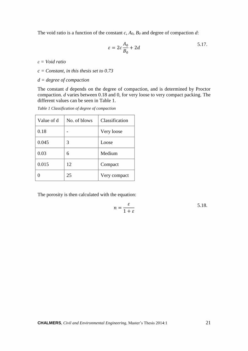
The void ratio is a function of the constant c, A0, B0 and degree of compaction d:
𝜀 = 2𝑐
𝐴0
𝐵0+ 2𝑑
5.17.
ε = Void ratio
c = Constant, in this thesis set to 0.73
d = degree of compaction
The constant d depends on the degree of compaction, and is determined by Proctor
compaction. d varies between 0.18 and 0, for very loose to very compact packing. The
different values can be seen in Table 1.
Table 1 Classification of degree of compaction
Value of d No. of blows Classification
0.18 - Very loose
0.045 3 Loose
0.03 6 Medium
0.015 12 Compact
0 25 Very compact
The porosity is then calculated with the equation:
𝑛 =𝜀
1 + 𝜀
5.18.

22 CHALMERS, Civil and Environmental Engineering, Master’s Thesis 2014:1
6 Methodology laboratory work
Laboratory work has been done to calculate hydraulic conductivity in several ways.
The grain size analysis has been used to calculate a hydraulic conductivity by the use
of the Hazen equation and the Gustafson equation. It is also used as part of the shape
factor in the Kozeny-Carman equation. The compact density, bulk density, water
content and colon test have all been used to determine the porosity, which is an
important part of the Kozeny-Carman equation. The permeameter test has been used
to calculate the hydraulic conductivity experimentally.
6.1 Grain size analysis
The grain size analysis is done through sieving. Several sieves with mesh sizes
ranging from 20 mm to 0.063 mm are used. The soil material is first dried in an oven
at 105° C to remove water content, weighed, and then washed in a fine-grained sieve
to remove material smaller than 0.063 mm. The material is then dried and weighed to
calculate the amount that has been washed away. The material is then sieved. The
amount of material on each sieve is weighed and the percentage of the entire material
that is passing through each sieve can be entered into a grain size diagram. The soil
type is determined by noting how much of the material that contains of sand, gravel,
silt or clay.
When reviewing the grain size diagrams, some things can be noted by observing the
curve. A multi-graded material like a glacial till, containing all different grain sizes, is
usually normally distributed and the curve has a slight inclination. In contrast, a more
one-graded material has a much steeper inclination.
If the soil material contains a high amount of fine material that passes through the
smallest 0.063 mm sieve, a sedimentary analysis is done to determine the fine soil
distribution.
To determine the soil type, the amount of gravel, sand and fine material is determined,
in percentages, and by entering these percentages into a nomogram the soil type can
be determined, see Figure 8 (Larsson, 2008).
Figure 8 Nomogram for the classification of mineral soil after grain size distribution (Larsson 2008)

CHALMERS, Civil and Environmental Engineering, Master’s Thesis 2014:1 23
The percentage of gravel is placed in the side marked 1, the percentage of sand in the
side marked 2, and the fine material in the side marked 3. This nomogram does not
determine if the fine material is silt or clay, as a sedimentary analysis is necessary to
determine the fine material.
6.2 Permeameter test
To evaluate hydraulic conductivity with laboratory methods, the constant head
method or the falling head method can be used. When the constant head method is
used, water is moved through a soil under a constant head condition. The volume of
water passing through the sample is measured and a hydraulic conductivity can be
calculated. When the falling head method is used, the soil sample is saturated to a
certain head and water then flows through the water without maintaining a constant
head (Fagerström & Wiesel, 1972).
For these laboratory tests, the constant head method has been used. When measuring
hydraulic conductivity with the constant head method, a permeameter is used. The
packed and saturated soil material is placed inside a container. The time it takes for a
certain volume of water to move through the material is measured and thus the flow
can be calculated in cm3/s. The water pillar is measured to calculate the pressure.
This, along with the dimensions of the container is used to calculate the hydraulic
conductivity with the use of equation 6.1.
𝐾 =𝑉 ∙ 𝑙
𝐴𝑠 ∙ 𝑡 ∙ ℎ∙ 10−2 6.1.
K = Hydraulic conductivity [m/s]
V = Volume of water flowing through the sample [cm3]
l = Length of sample [cm]
As = Cross sectional area of sample [cm2]
t = Time of water flowing through the sample [s]
h = Height of water pillar [cm]
6.3 Compact density
To determine the compact density of a soil sample, a pycnometer test can be used
(Sällfors, 1993). The volume of the pycnometer is determined as well as the weight.
The pycnometer is filled with a liquid (water) of known density and weighed. A soil
sample, which has been dried to 105°C and then grinded, is put into the pycnometer,
which is weighed. The pycnometer is then filled with water and weighed. Both the
water used and the saturated soil sample has been de-aered to remove all possible air
bubbles. The volume of the water can now be calculated. The difference between the
volume of the pycnometer and the volume of the water gives the volume of the soil
sample. The compact density is thus calculated by equation 6.2.

24 CHALMERS, Civil and Environmental Engineering, Master’s Thesis 2014:1
𝜌𝑠 =𝑚𝑠𝑜𝑖𝑙
𝑉𝑠𝑜𝑖𝑙=
𝑚𝑠𝑜𝑖𝑙
𝑉𝑝𝑦 − 𝑉𝑤 6.2.
ρs = Compact density of soil sample [g/cm3]
msoil = Weight of soil sample [g]
Vsoil = Volume of soil sample [cm3]
Vpy = Volume of pycnometer [cm3]
Vw = Volume of water [cm3]
6.4 Bulk density
To determine the bulk density of the sample, Archimedes principle is used (Pusch,
1973). The saturated soil sample is placed in a container. The container has
previously been weighed empty and filled with mineral turpentine. The container with
the soil sample is weighed in air and filled with mineral turpentine, and the bulk
density can then be calculated by equation 6.3:
𝜌 =𝑚3 − 𝑚1
𝑚3 − 𝑚4 − 𝑚1 + 𝑚2∙ 𝜌1 6.3.
ρ = Bulk density of soil sample [g/cm3]
ρ1 = Density of mineral turpentine [g/cm3]
m1 = Weight of empty container [g]
m2 = Weight of container and mineral turpentine [g]
m3 = Weight of soil sample [g]
m4 = Weight of soil sample and mineral turpentine [g]
The mineral turpentine is used since it does not penetrate the saturated soil sample
and will evaporate when the soil sample is taken out of the liquid.
6.5 Porosity
The measurements to calculate the porosity has been done in two different ways,
depending on the methods used for the soil sampling. The porosity of the samples
from Korsvägen has been calculated by using specific gravity and water content and
the porosity of the samples from Skansen Lejonet has been calculated by colon tests.

CHALMERS, Civil and Environmental Engineering, Master’s Thesis 2014:1 25
6.5.1 Porosity measurements on Skansen Lejonet samples
Since the samples from Skansen Lejonet was taken with a sampling method that did
not preserve the original water content, a method that compares the relationship
between masses instead of between densities have been used, equation 6.6, as the
other method requires water content to calculate the porosity (see equation 6.4)
(Fransson & Nordén, 1996). The sample is packed up to a mark in a cylinder, which
has been weighed empty and filled with de-aered water to the mark. The material is
weighed and saturated with de-aered water and the total mass is weighed. By using
the following equation, the porosity can then be measured, see equation 6.4:
𝑛 =𝑚8 − 𝑚7
𝑚6 − 𝑚5∙ 100 6.4.
n = Porosity [-]
m5 = Mass of cylinder [g]
m6 = Mass of water up to mark and cylinder [g]
m7 = Mass of soil up to mark and cylinder [g]
m8 = Mass of water and soil up to mark and cylinder [g]
6.5.2 Porosity measurements on Korsvägen samples
To determine the porosity, water content, compact density and bulk density has been
used as seen in equation 6.5 (Larsson, 2008):
𝑛 = (1 −
𝜌
𝜌𝑠(𝑤 + 1)) 6.5.
n = Porosity [-]
ρ = Bulk density of soil sample [g/cm3]
ρs = Compact density of soil sample [g/cm3]
w = Water content [%]

26 CHALMERS, Civil and Environmental Engineering, Master’s Thesis 2014:1
The bulk density and compact density is determined as described in chapter 6.3 and
6.4. The water content is determined by weighing a soil sample before and after it has
been dried for 24 hours in 105°C (Larsson, 2008), see equation 6.6:
𝑤 =𝑚𝑤
𝑚𝑠⁄ ∙ 100 6.6.
w = Water content [%]
mw = Mass of water [g]
ms = Mass of soil [g]

CHALMERS, Civil and Environmental Engineering, Master’s Thesis 2014:1 27
7 Execution and observations
7.1 Soil sampling
For the tests executed in this thesis, three different methods have been used to collect
samples. The sampling was performed on March 25-26, 2013.
7.1.1 Skansen Lejonet
At Skansen Lejonet, five boreholes were made, OC4008, OC4009, OC4010, OC4011
and OC4012, see Figure 9. Both the previous and current boreholes can be seen in
Figure 10.
Figure 9 Map over Skansen Lejonet with boreholes marked in red (Google Maps, 2013b). Modified.

28 CHALMERS, Civil and Environmental Engineering, Master’s Thesis 2014:1
Figure 10 The boreholes at Skansen Lejonet, with the mountain block in the center of the picture. The
previous boreholes are marked in black and the current in red (SWECO, 2013c).
At Skansen Lejonet, the soil material was flushed up with compressed air and water,
see Figure 11. The tip of the drill were perforated with oval holes approximately
20x40 millimetres, see Figure 12. This sample method provides more disturbed
samples than when using a moraine sampler. As the material is flushed with water,
the original water content of the soil cannot be calculated.
Figure 11 The hammer drill used at Skansen Lejonet
Figure 12 The tip of the
drill used at Skansen
Lejonet

CHALMERS, Civil and Environmental Engineering, Master’s Thesis 2014:1 29
At the same time, WSP took samples from the same boreholes, which are the ones
with the same borehole id-number mentioned in chapter 8.3. However, for the tests
executed in this thesis, care was taken to collect samples that were as complete as
possible and included all of the finer material. To achieve this, the material that was
flushed up was collected in fibre cloth. This explains the differences in the different
results from the same boreholes.
When drilling at Skansen Lejonet, the sand layer under the clay was found to be
small, not more than one or a couple of meters. There was a high content of fine sand
and silt and a smaller content of gravel and coarse sand. The small content of gravel
probably means that in this case, this method of sampling did not miss the coarser
material.
7.1.2 Korsvägen
At Korsvägen, samples were collected at two boreholes, KK5038 and KK5040, see
Figure 13. When comparing the test results from this sampling to previous sampling,
the borehole closest to KK5038 is KK4012, only a few meters away. The borehole
closest to KK5040 is KK4003 approximately 15 meters away and KK4014, 20 meters
distance from KK5040 and 20 meters distance from KK5038.
Originally, a moraine sampler was going to be used in the sampling, but it broke
down during sampling, and only the first sample (KK5038-1) at borehole KK5038
were collected with this sampler. The moraine sampler has an inner diameter of 42
mm and collects samples similar to a piston sampler, in order to achieve as
undisturbed samples as possible. After the moraine sampler broke down, a barrel
sampler was used to collect the rest of the samples. The barrel sampler has an inner
diameter of 30 mm.
Figure 13 Map showing the boreholes at Korsvägen. Current sampling is marked in red and previous
sampling in green. The pumping well is marked in blue (Google Maps, 2013a) (Modified).
KK5038
KK4003 KK5040
KK4012
KK4014
KK4007
KK4001
KK4002
KK4004
KK4005
KK4008 KK4009
KK4010 KK4011
KK4015
KK4016
KK4001H

30 CHALMERS, Civil and Environmental Engineering, Master’s Thesis 2014:1
The samples were to various degrees rather heterogenous, with all sorts of grain sizes
from clay to gravel. It is worth noting that in several of the samples, gravel larger than
8 millimetres were found, the largest stone as big as 23 millimetres.
7.2 Previous sampling
Previously, soil samples have been retrieved from the boreholes to perform grain size
analyses. Hydraulic tests such as slug tests, pumping tests and measurements of the
recharge have also been performed.
7.2.1 Soil sampling for grain size analyses
The soil samples used in this thesis have been compared to previous grain size
analyses taken in nearby boreholes. The boreholes are mostly 2 inch-pipes, and in a
few cases hammer boreholes into bedrock with 4.5 inch-pipes. The previous soil
samples used for grain size analyses were taken with perforated pipes. These pipes are
perforated with holes spanning 8 millimetres in diameter, see Figure 15. The soil
enters the pipe through these holes. A hose with compressed air or water is used to
blow out the soil material, which is collected in a vessel, and the wanted amount of
material is taken from the vessel, see Figure 14. Using this method means that coarser
fractions than 8 millimetres of the soil material are not part of the sample. The finest
fractions are also removed during sampling. Depending on if the material is relatively
single-graded or multi-graded this may lead to the grain size analysis being skewed. A
single-graded sand may very well give good results, as the majority of the material is
captured by this sample methodology, but a more multi-graded soil may give
misleading results if the coarser and finer fractions that are being left out by this type
of sampling makes up a larger part of the material.
Air or
water After pipe is
driven into the
ground Samples
Figure 14 Principal sketch of the sampling method used in previous
sampling (Gustavsson, 2005)
Figure 15 Drawing of a perforated
pipe (Andersson, et al., 1984)

CHALMERS, Civil and Environmental Engineering, Master’s Thesis 2014:1 31
7.2.2 Slug tests
As a complement to the grain size analyses, hydraulic tests have also been done, both
at Skansen Lejonet and at Korsvägen. Four tests were performed at Skansen Lejonet
and fourteen tests were performed at Korsvägen in the 2 inch-pipes. A certain volume
of water was added to the pipes, and the change in pressure at the ground water Table
was measured both manually during the first 10 minutes, and with a pressure
transmitter. The slug tests were evaluated with the Cooper-Bredehoeft-Papadopulos
method.
7.2.3 Pumping tests
When performing the pumping tests, a general assessment was made for which
observation wells can be influenced during the interference tests. The properties of the
pumping well and the aquifers are evaluated and the boundary conditions are
determined to create a model of the aquifer. The response from the observation wells
are then studied and evaluated. The pumping tests were performed with wells with
adapted filter widths. The observation wells are drilled down to the glacial till on top
of the bedrock so that the filter part of the wells is placed into the conductive friction
material. Just as with the boreholes, there are 8 mm holes perforated across the mantel
area. The inside diameter of the casing tubes are approximately 52 mm and the
diameter of the filter is approximately 50 mm. The Cooper-Jacob method was used to
evaluate the results (SWECO, 2013b).
The pumping test at Skansen Lejonet was performed in April 2013 in the well
OC4001B (see Figure 10). At the beginning of the test there was heavy rainfall that
affected the response in four of the observation wells. The measurements from these
wells were consequently not used in the analysis. Five observation wells in the lower
aquifer to the northwest responded to the pumping, while the well in the upper aquifer
to the west did not respond. The results showed that the aquifer probably was limited
in a longitudinal extent, confined to a few 100 meters.
At Korsvägen, a pumping test was performed in January 2013 in the well KK4001B
(see Figure 13). Six of the observation wells around Korsvägen and south responded
to the pumping. An observation well north-northwest of the area does also show a
response but the observation well to the north does not show a clear recharge. To the
east, towards Liseberg, none of the four observation wells showed any response,
however a pumping test performed in 2005 indicated some hydraulic contact, which
cannot be disregarded.
7.3 Laboratory work
The laboratory work was performed between April and June of 2013 in the
geotechnical and hydrogeological laboratory at Chalmers University of Technology.
Due to the differences in sampling method, mainly that the sampling at Skansen
Lejonet did not preserve the original water content, different laboratory tests were
performed on the samples. The permeameter test requires samples to be at least a
volume of one litre. Four samples were large enough to perform this test, see
description in chapter 6.2. The samples were packed to simulate in-situ conditions.
During the test, the flow was measured until it had reached a steady state, and several

32 CHALMERS, Civil and Environmental Engineering, Master’s Thesis 2014:1
values in a row were the same within a margin of ±1%. The test setup can be seen in
Figure 16.
All samples were sieved to perform a grain size analysis, see description in chapter
6.1. Many of the samples from Korsvägen had a large amount of fine material, but
these samples were prematurely destroyed before a sedimentation analysis could be
done.
The porosity measurements were done in two different ways, described in chapter 6.5.
The methods used for samples were the water content cannot be determined requires
the samples to be of a certain volume, which is why experimental porosity values are
missing for some of the samples from Skansen Lejonet. This method is also more
likely to have uncertainties since it is less precise. The porosity values from
Korsvägen are therefore probably more reliable than the values from Skansen
Lejonet. For the Korsvägen samples, pycnometers were used to determine compact
and bulk density, see Figure 16.
7.4 Calculations of hydraulic conductivity
The three different empirical methods that are described in chapter 3 have all been
used to calculate the hydraulic conductivity. Gustafson and Hazen both depend on
grain size, more particularly the parameters d60 and d10 and the relationship between
these. In the cases where d10 were smaller than 0,063 millimetres the values have been
extrapolated with a log-normal distribution using the Excel add-on @risk.
The Kozeny-Carman method also uses d60 and d10, but in addition to this, porosity is
also used.
Figure 16 From left to right, permeameter test, pycnometer with soil and water, pycnometer
with soil and mineral turpentine

CHALMERS, Civil and Environmental Engineering, Master’s Thesis 2014:1 33
8 Results
The results from the porosity calculations and the hydraulic conductivity calculations
are presented below. The results from previous sampling are also presented in this
chapter.
8.1 Porosity
The porosities have been calculated experimentally in two different ways depending
on the origin of the samples (see chapter 6.5 for description). The porosity
measurements on the samples from Korsvägen is likely to have less uncertainties than
the samples from Skansen Lejonet, where the measurements are less exact and the
samples are more disturbed than the Korsvägen samples. The porosity has not been
calculated experimentally for three of the Skansen Lejonet samples due to the
insufficiently small sample size in these cases.
The porosity has also been calculated from grain size analysis, as described in chapter
5.4. In this thesis, no Proctor compaction has been done and the optimal water content
is thus not determined. The degree of compaction is therefore not determined.
However, the porosities for different d-values have been calculated and compared to
the experimentally obtained porosities. The porosities from Skansen Lejonet can be
seen in Table 2. The degree of compaction was chosen depending on the soil type and
the experimentally obtained porosity. As it is not likely that different levels of the
same borehole have different degrees of compaction, a degree of compaction where
the porosity calculated from this correspond best to the experimentally obtained
porosity on average for the borehole have been chosen. Table 2 and 3 shows the
different porosities based on a span of compaction degrees. The chosen porosity is
marked in grey and is the one used to calculate hydraulic conductivity with the
Kozeny-Carman equation, KKC1.

34 CHALMERS, Civil and Environmental Engineering, Master’s Thesis 2014:1
Table 2 The porosities from Korsvägen depending on degree of compaction, as well as experimentally
calculated. The porosity used in the calculations is marked in grey. The uniformity coefficient, Cu, is
also presented.
For the porosities from Skansen Lejonet the theoretical porosities closest to the
experimentally varies from Very Loose to Medium.
When comparing the experimental values from Korsvägen with the closest
corresponding theoretical value, the degree of compaction varies a lot. The chosen
degree of compaction for the porosities is Compact, however the porosity at KK5040-
1 is so different from the experimentally obtained one that Loose is chosen instead.
This borehole level is in this case seen as an anomaly.
Skansen
Lejonet
V.
loose Loose Medium
Com-
pact
V.
compact Exp Soil type
Cu
OC4008-1 0.31 0.16 0.14 0.11 0.09 0.28
Gravelly
sand
23.8
OC4008-2 0.36 0.23 0.21 0.19 0.17
Gravelly
sand
9.8
OC4008-3 0.34 0.19 0.17 0.15 0.13
Gravelly
sand
15.0
OC4009-1 0.45 0.36 0.34 0.33 0.32 0.34 Sand 2.6
OC4009-2 0.43 0.33 0.32 0.30 0.29 0.33 Sand 3.4
OC4010 0.44 0.34 0.33 0.32 0.30 0.34 Sand 3.0
OC4011-1 0.46 0.37 0.36 0.35 0.33 Sand 2.3
OC4011-2 0.45 0.35 0.33 0.32 0.31 0.34 Sand 2.9
OC4012 0.45 0.35 0.34 0.33 0.31 0.34 Sand 2.7

CHALMERS, Civil and Environmental Engineering, Master’s Thesis 2014:1 35
Table 3 The porosities from Korsvägen depending on degree of compaction, as well as experimentally
calculated. The porosity used in the calculations is marked in grey.The uniformity coefficient, Cu, is
also presented.
Two factors can be seen that influences the porosity, soil type and uniformity
coefficient. When calculating the theoretical porosity, the uniformity coefficient
influences the value quite a lot. A multi-graded soil gives a low porosity as smaller
grains fits into the voids left by larger grains. For soil with a high content of fine
material, the material is probably more compacted whereas for coarser material the
packing is looser. This influences what grade in the compaction index the porosity
will lie in. A graph of how the different porosities vary can be seen in appendix 4. The
impact of the degree of compaction for the hydraulic conductivity can be seen in
appendix 3.
8.2 Hydraulic conductivity
The hydraulic conductivity has been calculated with four different methods, a short
description of these can be seen in Table 4. There are two different calculations based
on the Kozeny-Carman method, as the porosity is calculated in two different ways,
see chapter 6.5.
Korsvägen V.
loose Loose Medium Compact
V.
compact Exp.
Soil type
Cu Borehole
KK5040-1 0.30 0.14 0.12 0.10 0.07 0.20
Gravelly
sand 31.1
KK5040-2 0.41 0.30 0.29 0.27 0.26 0.27
Gravelly
silty sand 4.5
KK5040-3 0.40 0.29 0.27 0.26 0.24 0.19
Sandy
silt/clay 5.2
KK5038-1 0.42 0.31 0.29 0.28 0.26 0.27
Clayey silty
sand 4.2
KK5038-2 0.33 0.18 0.16 0.14 0.11 0.18
Clayey silty
sand 17.5

36 CHALMERS, Civil and Environmental Engineering, Master’s Thesis 2014:1
Table 4 The different methods used to calculate the hydraulic conductivity, K.
Name Abbreviation Parameters
Hazen KH Grain size, empirical constant
Gustafson KG Grain size, uniformity coefficient
Kozeny-Carman KKC1 Grain size, shape factor, tortuosity, theoretical porosity
Kozeny-Carman KKC2 Grain size, shape factor, tortuosity, experimental porosity
Permeameter Kexp Flow
The hydraulic conductivity results are shown in Table 5. The permeameter test has
only been performed on four samples, and only three of these gave a result. The
Kozeny-Carman hydraulic conductivity calculated from experimental porosity, KKC2,
have not been calculated in three cases due to the lack of porosity calculations in these
cases. To show the difference between the results based on Gustafson and the results
based on Kozeny-Carman, the ratio, KG/KKC1, between these two methods are also
shown.

CHALMERS, Civil and Environmental Engineering, Master’s Thesis 2014:1 37
Table 5 Hydraulic conductivity measurements from four different methods.
Borehole KH KG KKC1 KKC2 Kexp
KG/K
KC1
Soil type
Skansen Lejonet [m/s] [m/s] [m/s] [m/s] [m/s]
OC4008-1 4.6E-05 2.2E-05 2.7E-06 1.6E-06 2.4E-07 8.20
Gravelly
sand
OC4008-2 8.8E-05 7.3E-05 3.4E-05 - 12.65
Gravelly
sand
OC4008-3 1.2E-04 7.5E-05 1.9E-05 - 31.09
Gravelly
sand
OC4009-1 2.0E-04 2.8E-04 1.3E-04 1.2E-04 - 2.17 Sand
OC4009-2 2.0E-04 2.7E-04 9.2E-05 1.1E-04 - 2.44 Sand
OC4010 9.4E-05 1.3E-04 5.3E-05 5.9E-05 No flow 2.13 Sand
OC4011-1 5.7E-05 8.3E-05 4.4E-05 5.3E-06 1.88 Sand
OC4011-2 5.0E-05 7.2E-05 3.0E-05 3.2E-05 - 2.05 Sand
OC4012 4.9E-05 7.0E-05 3.2E-05 3.1E-05 1.6E-06 2.20 Sand
Korsvägen
KK5040-1 2.9E-05 1.3E-05 8.30E-08 2.3E-07 - 203.00
Gravelly
sand
KK5040-2 1.9E-05 2.3E-05 4.4E-06 4.3E-06 - 5.24
Gravelly
silty sand
KK5040-3 2.4E-06 1.9E-06 6.0E-08 8.0E-08 - 8.73
Sandy
silt/clay
KK5038-1 1.6E-05 1.9E-05 3.0E-06 3.7E-06 - 5.98
Clayey
silty sand
KK5038-2 4.6E-06 2.7E-06 2.4E-08 2.7E-07 - 45.17
Clayey
silty sand
It is clear that Gustafson and Hazen gives the highest values, sometimes with a
difference of several orders of magnitude between the highest and the lowest values.
The lowest values are the ones experimentally calculated from permeameter tests,
Kexp, and the Kozeny-Carman equation with porosities calculated from grain size,
KKC1.
Skansen Lejonet shows higher hydraulic conductivity than Korsvägen. The values at
Skansen Lejonet spans between 10-4 and 10-7 m/s and at Korsvägen between 10-5 and

38 CHALMERS, Civil and Environmental Engineering, Master’s Thesis 2014:1
10-8 m/s. The grain size curves for Skansen Lejonet can be seen in appendix 1, and the
grain size curves for Korsvägen in appendix 2. In appendix 2, some values have been
extrapolated with a log-normal distribution.
8.3 Previous sampling – grain size analysis
The results from previous samplings are shown in Tables 6 and 7 (SWECO, 2013a)
(SWECO, 2013c). The previous analyses have used the Gustafson equation, KG, to
calculate hydraulic conductivity. To compare the different results, the hydraulic
conductivity has now also been calculated with the Hazen equation, KH, and the
Kozeny-Carman equation, KKC1. The porosities used for the Kozeny-Carman equation
are empirically calculated from grain size. The degree of compaction has been chosen
depending on soil type, with the values from current sampling as model. This might
make the Kozeny-Carman results somewhat uncertain. The uniformity coefficient,
CU, is also shown. The boreholes at Skansen Lejonet that are the same as the ones
tested in this thesis are marked with italic letters in Table 6.

CHALMERS, Civil and Environmental Engineering, Master’s Thesis 2014:1 39
Table 6 Hydraulic conductivity from boreholes at Skansen Lejonet calculated with three different
methods, and the uniformity coefficient CU.
Borehole Level KH KG KKC1 CU
Skansen Lejonet [m] [m/s] [m/s] [m/s] [-]
OC4001H 7-8 8.2E-03 1.1E-02 3.7E-03 3.1
OC4001H 8-9 5.1E-04 6.6E-04 1.8E-04 4.0
OC4001H 9-10 1.3E-03 1.3E-03 1.2E-04 6.7
OC4001H 10-11 1.0E-03 1.3E-03 2.3E-04 4.7
OC4001H 11-12 1.7E-03 2.3E-03 6.5E-04 3.4
OC4001 18-19 5.3E-05 7.7E-05 3.5E-05 2.6
OC4001 19-19.3 6.9E-05 1.0E-04 5.2E-05 2.3
OC4002 14-15 4.6E-05 6.5E-05 2.6E-05 3.0
OC4002 15-16 1.4E-04 2.0E-04 7.9E-05 3.0
OC4002 16-17 4.7E-05 6.1E-05 1.3E-05 4.2
OC4002 17-18 1.4E-04 1.4E-04 1.7E-05 6.8
OC4002 18-19 4.6E-05 5.4E-05 1.1E-05 5.1
OC4003 12-13 2.9E-05 4.0E-05 1.6E-05 3.4
OC4003 13-14 7.4E-05 1.1E-04 5.2E-05 2.5
OC4005 1-2 2.9E-03 3.2E-03 3.5E-03 1.0
OC4006 0-2.7
OC4007 7-8 7.4E-05 1.1E-04 4.7E-05 2.8
OC4007 8-9 7.2E-04 1.0E-03 3.7E-04 3.2
OC4007 9-10 1.2E-03 1.6E-03 5.5E-04 3.4
OC4008 16.0-17.0 3.5E-03 4.9E-03 1.5E-03 3.2
OC4008 15.0-16.0 1.9E-05 5.9E-06 1.9E-09 45.8
OC4008 15.5-16.5 8.2E-05 7.8E-05 7.3E-06 7.7
OC4009 8-9 2.0E-04 2.9E-04 1.2E-04 2.8
OC4009 9-10 3.3E-04 4.2E-04 1.1E-04 4.2
OC4010 11.6-12.6 6.3E-05 9.2E-05 4.3E-05 2.6
OC4011 13.1-14.1 5.0E-05 7.2E-05 3.0E-05 2.9
OC4012 13.4-14.4 7.6E-05 1.1E-04 5.1E-05 2.6
Just as in previous results, Hazen and Gustafson show fairly similar results where
Kozeny-Carman gives lower hydraulic conductivity than the other two. The hydraulic
conductivity at this location is rather high, with maximum values in orders of 10-2 and
10-3 m/s and ranging down to around 10-5 or 10-6 m/s in the case of KKC1.

40 CHALMERS, Civil and Environmental Engineering, Master’s Thesis 2014:1
In Table 7, the results from Korsvägen can be seen. At Korsvägen, some of the d10-
values are too small to have been determined from grain size analysis and was instead
extrapolated. This makes the results more uncertain. The samples were d10 is
extrapolated is marked with an asterisk in Table 7.

CHALMERS, Civil and Environmental Engineering, Master’s Thesis 2014:1 41
Table 7 Hydraulic conductivity from boreholes at Korsvägen calculated with three different methods,
and the uniformity coefficient CU.
Borehole Level KH KG KKC1 CU
Korsvägen [m] [m/s] [m/s] [m/s] [-]
KK4001 10-11 1.9E-09 3.2E-10 1.9E-15 125
KK4002* 10-11 4.6E-06 1.6E-06 8.7E-10 40
KK4003 9-10 2.9E-05 3.9E-05 1.2E-05 3.6
KK4003 10-11 2.9E-05 4.2E-05 2.0E-05 2.2
KK4003 11-12 7.4E-05 9.0E-05 1.9E-05 4.75
KK4004 13-14 1.4E-04 1.6E-04 2.5E-05 5.7
KK4004 14-15 9.4E-05 1.2E-04 2.8E-05 4.4
KK4004 15-16 9.4E-05 8.9E-05 8.3E-06 7.8
KK4004 16-17 1.4E-04 1.7E-04 3.9E-05 4.6
KK4004 17-18 1.2E-04 1.4E-04 3.2E-05 4.6
KK4004 18-19 1.2E-04 1.4E-04 3.2E-05 4.6
KK4004 19-20 2.9E-05 3.1E-05 3.4E-06 6.2
KK4005 12-13 1.4E-04 1.4E-04 1.4E-05 7.5
KK4005 13-14 7.4E-05 6.1E-05 3.3E-06 10.1
KK4005* 19-20 1.0E-05 1.5E-05 5.8E-06 2.7
KK4005 21-22 4.2E-05 5.9E-05 2.5E-05 2.8
KK4005 22-23 4.2E-05 5.8E-05 2.2E-05 3.2
KK4007* 9-10 4.6E-06 2.9E-06 3.7E-08 15.5
KK4008 20-21 9.4E-05 1.3E-04 5.0E-05 3.1
KK4008 21-22 5.7E-05 8.2E-05 3.9E-05 2.6
KK4010* 17-18 1.9E-05 2.6E-05 7.8E-06 3.3
KK4011* 1-1,6 4.6E-06 1.6E-06 8.7E-10 40
KK4012 17-18 5.7E-05 8.1E-05 3.4E-05 2.9
KK4012 20-21 7.4E-05 7.0E-05 6.4E-06 7.9
KK4014 5-6 2.9E-05 2.3E-05 1.0E-06 11
KK4014 10-11 2.9E-05 4.2E-05 1.7E-05 2.6
KK4014 11-12 4.2E-05 5.3E-05 1.3E-05 4.3
KK4015 7-8 4.2E-05 5.7E-05 1.9E-05 3.5
KK4015* 9-10 1.9E-05 2.7E-05 1.1E-05 2.5
KK4015 10-11 5.7E-05 8.2E-05 4.1E-05 2.4
KK4016 4.5-5.5 4.2E-05 4.9E-05 1.1E-05 5.2
KK4016 6-7 2.3E-04 2.8E-04 6.6E-05 4.5
KK4016* 7-8 4.6E-06 2.5E-06 1.5E-08 20
KK4016 8-9 2.9E-05 2.7E-05 1.8E-06 8
KK4001H 11-13 2.0E-04 6.5E-05 1.3E-07 43.1
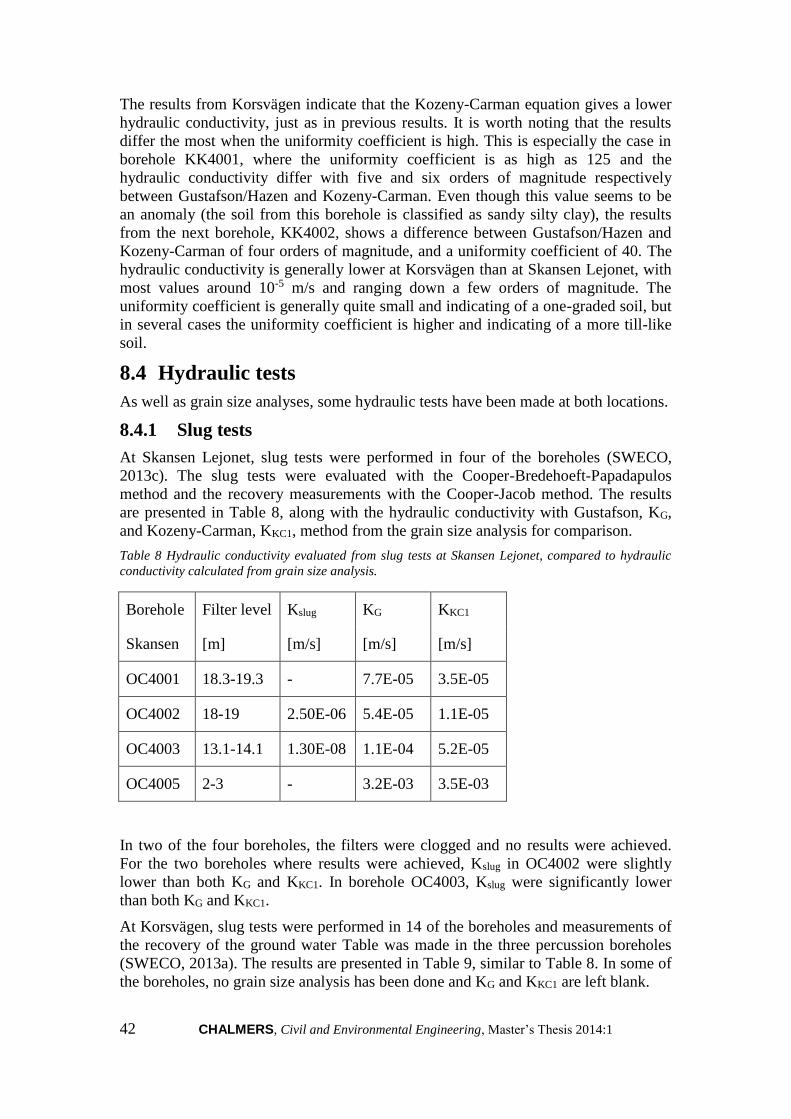
42 CHALMERS, Civil and Environmental Engineering, Master’s Thesis 2014:1
The results from Korsvägen indicate that the Kozeny-Carman equation gives a lower
hydraulic conductivity, just as in previous results. It is worth noting that the results
differ the most when the uniformity coefficient is high. This is especially the case in
borehole KK4001, where the uniformity coefficient is as high as 125 and the
hydraulic conductivity differ with five and six orders of magnitude respectively
between Gustafson/Hazen and Kozeny-Carman. Even though this value seems to be
an anomaly (the soil from this borehole is classified as sandy silty clay), the results
from the next borehole, KK4002, shows a difference between Gustafson/Hazen and
Kozeny-Carman of four orders of magnitude, and a uniformity coefficient of 40. The
hydraulic conductivity is generally lower at Korsvägen than at Skansen Lejonet, with
most values around 10-5 m/s and ranging down a few orders of magnitude. The
uniformity coefficient is generally quite small and indicating of a one-graded soil, but
in several cases the uniformity coefficient is higher and indicating of a more till-like
soil.
8.4 Hydraulic tests
As well as grain size analyses, some hydraulic tests have been made at both locations.
8.4.1 Slug tests
At Skansen Lejonet, slug tests were performed in four of the boreholes (SWECO,
2013c). The slug tests were evaluated with the Cooper-Bredehoeft-Papadapulos
method and the recovery measurements with the Cooper-Jacob method. The results
are presented in Table 8, along with the hydraulic conductivity with Gustafson, KG,
and Kozeny-Carman, KKC1, method from the grain size analysis for comparison.
Table 8 Hydraulic conductivity evaluated from slug tests at Skansen Lejonet, compared to hydraulic
conductivity calculated from grain size analysis.
Borehole Filter level Kslug KG KKC1
Skansen [m] [m/s] [m/s] [m/s]
OC4001 18.3-19.3 - 7.7E-05 3.5E-05
OC4002 18-19 2.50E-06 5.4E-05 1.1E-05
OC4003 13.1-14.1 1.30E-08 1.1E-04 5.2E-05
OC4005 2-3 - 3.2E-03 3.5E-03
In two of the four boreholes, the filters were clogged and no results were achieved.
For the two boreholes where results were achieved, Kslug in OC4002 were slightly
lower than both KG and KKC1. In borehole OC4003, Kslug were significantly lower
than both KG and KKC1.
At Korsvägen, slug tests were performed in 14 of the boreholes and measurements of
the recovery of the ground water Table was made in the three percussion boreholes
(SWECO, 2013a). The results are presented in Table 9, similar to Table 8. In some of
the boreholes, no grain size analysis has been done and KG and KKC1 are left blank.

CHALMERS, Civil and Environmental Engineering, Master’s Thesis 2014:1 43
Table 9 Hydraulic conductivity evaluated from slug test at Korsvägen, compared to hydraulic
conductivity calculated from grain size analysis.
Borehole Filter level Kslug KG KKC1
Korsvägen [m] [m/s] [m/s] [m/s]
KK4001 10.5-11.5 4.7E-09 3.2E-10 1.9E-15
KK4002 9.75-10.75 3.6E-10 1.6E-06 8.7E-10
KK4003 11.2-12.2 3.0E-05 9.0E-05 1.9E-05
KK4004 18.9-19.9 6.8E-10 3.1E-05 3.4E-06
KK4005 21.7-22.7 6.3E-10 5.8E-05 2.2E-05
KK4006 12.2-13.2 3.2E-07 - -
KK4007 9-10 4.4E-07 2.9E-06 3.7E-08
KK4009 20-21 1.9E-05 - -
KK4010 19.3-20.3 - 2.6E-05 7.8E-06
KK4011 0.5-1.5 1.9E-05 1.6E-06 8.7E-10
KK4013 17-18 1.2E-04 - -
KK4014 11.3-12.3 1.8E-05 5.3E-05 1.3E-05
KK4015 10-11 1.3E-05 8.2E-05 4.1E-05
KK4016 8.5-9.5 8.3E-07 2.7E-05 1.8E-06
8.4.2 Pumping tests
The analysis from the pumping test at Skansen Lejonet shows that a model with a 30-
meter wide channel can explain the response at the first 50 minutes, where the flow is
linear. The drawdown rate is then lowered which is interpreted as leakage from the
friction material surrounding the channel. The analysis shows that the channel
probably represents a limited aquifer in a longitudinal extent, confined to a few 100
meters.
The result of the pumping tests shows that the lower aquifer is probably closed. The
transmissivity for the channel is rather high, 1.2*10-3 m2/s. Outside the channel the
transmissivity is estimated to approximately 3*10-6 – 3*10-5 m2/s. There are large
uncertainties when estimating the height of the ground water zone, but a rough
estimation based on sounding is a depth of 1 meter. The hydraulic conductivity inside

44 CHALMERS, Civil and Environmental Engineering, Master’s Thesis 2014:1
the channel is then 1.2*10-3 m/s, and the hydraulic conductivity outside is between
3*10-6 – 3*10-5 m/s.
The pumping test at Korsvägen showed a large influence area, probably several
hundreds of meters (SWECO, 2013b). The tests showed a probable connection
between the lower and middle ground water zone. Probably, the lower zone is also
hydraulically connected to the upper zone and the bedrock aquifer. The transmissivity
was calculated to be between 0.9 – 2 *10-4 m2/s. As the height of the ground water
zone was approximated to 6 meters, the hydraulic conductivity then becomes between
1.5 – 3.3 *10-5 m/s.
8.5 Statistical analysis
A statistical analysis has been performed to compare the different methods for
measuring hydraulic conductivity. The hypothesis is that the methods for measuring
hydraulic conductivity, Kozeny-Carman, Hazen and Gustafson, are significantly
different from each other, and that the results do not differ because of random
differences in the samples. This has been tested with an ANOVA single factor
analysis, see appendix 5. The analysis shows that with 97.8% certainty, the methods
are significantly different. This means that the Kozeny-Carman equation will give a
different result than Gustafson. However, the Hazen and Gustafson methods are not
significantly different from each other.

CHALMERS, Civil and Environmental Engineering, Master’s Thesis 2014:1 45
9 Evaluation of results
The four different methods for estimating hydraulic conductivity used in this thesis,
Kozeny-Carman, Hazen, Gustafson and experimental, provides different values with
some clear trends. To illustrate the differences between the methods, the results from
the current sampling have been plotted in a column chart. As the difference in
magnitude is the most interesting to see, the y-scale is logarithmic and reversed. This
means that the lowest conductivities have the highest bars in these charts, and vice
versa.
The results from Skansen Lejonet are presented in Figure 17.
Figure 17 Comparison of the results from Skansen Lejonet of the hydraulic conductivity with different
methods. The highest bars show the lowest conductivities.
The soil at Skansen Lejonet is generally more one-graded, which can be seen in these
results. The exceptions for this are partly in borehole OC4008 and partly in the
permeameter results. The Kozeny-Carman equation gives up to one and a half order
of magnitude difference in this borehole, which differ from the other boreholes, were
the results are almost similar.
1,E-07
1,E-06
1,E-05
1,E-04
1,E-03
1,E-02
1,E-01
1,E+00
K-Kozeny-Carman 1
K-Kozeny-Carman 2
K-Hazen
K-Gustafson
K-experimental

46 CHALMERS, Civil and Environmental Engineering, Master’s Thesis 2014:1
The results from Korsvägen are presented in Figure 18.
Figure 18 Comparison of the results from Korsvägen of the hydraulic conductivity with different
methods. The highest bars show the lowest conductivities
The results at Korsvägen show some differences between the different methods.
Hazen and Gustafson are consistently fairly similar, which also corresponds to the
statistical analysis that showed no significant differences between the methods. They
are also consistently higher than Kozeny-Carman. The more multi-graded soil at
Korsvägen is evident as the results from Korsvägen show the largest differences
between calculation methods, despite using the same sampling method. The
differences vary between one up to almost three orders of magnitude. A discussion of
the permeameter result will follow.
9.1 The effect of porosity on Kozeny-Carman results
When comparing the two different Kozeny-Carman results, KKC1 are sometimes lower
than KKC2. KKC1 is the hydraulic conductivity when using the theoretically calculated
porosities and KKC2 is the hydraulic conductivity when using the experimentally
obtained porosities. This difference is especially clear when the uniformity coefficient
is high. As can be seen in Table 7, chapter 8.3, there are some high CU-values that
lead to a difference between the two methods of many orders of magnitude. The most
extreme case is in borehole KK4001 where the uniformity coefficient is 125.
However, the soil from this borehole is classified as sandy silty clay, and the value
can be viewed as an anomaly. Even without this extreme value, there are results from
Korsvägen with uniformity coefficients up to 40, which leads to a difference of four
orders of magnitude between Kozeny-Carman and Gustafson, from 10-10 to 10-6 at for
example borehole KK4002 and KK4011. The hydraulic conductivity is thus almost
ten thousand times higher when using KG than KKC, obviously one of these values is
not realistic. An important thing to take into consideration is that some of the D10-
values at Korsvägen are extrapolated and thus uncertain.
1,E-08
1,E-07
1,E-06
1,E-05
1,E-04
1,E-03
1,E-02
1,E-01
1,E+00
KK5040-1 KK5040-2 KK5040-3 KK5038-1 KK5038-2
K-Kozeny-Carman 1
K-Kozeny-Carman 2
K-Hazen
K-Gustafson

CHALMERS, Civil and Environmental Engineering, Master’s Thesis 2014:1 47
When using the theoretically calculated porosities, two parameters seem to influence
the value. The degree of compaction depends a lot on the soil type, for example a
clayey soil is more compacted than a granular soil. Obviously this also influences the
porosity, as the voids between grains are smaller if the grains are smaller and vice
versa. In this thesis, the degree of compaction has not been the focus, but in
retrospect, this is something that could have been worth studying a lot more. When
calculating the porosities theoretically for the previous sampling, a rough estimation
of the degree of compaction from the soil type has been done. The comparison
between experimentally calculated porosities and the theoretically calculated ones
from current sampling has been used as a model to determine the degree of
compaction from the soil type. For example, in the borehole KK5040-2 the
experimental value was 0.27. This corresponds to the value when the degree of
compaction is “Compact” (12 blows with the Proctor compaction). As can be seen in
Table 10, the values fits better in some cases than in other, but a rough estimation can
be made.
Table 10 Example of different porosities based on various degree of compaction and experimental
values. The values marked in grey are the porosities that best correspond to the experimental values.
There are however only a few samples which makes the comparison somewhat
uncertain and arbitrary. Using experimentally calculated porosities as a key to study
how the soil type determines the degree of compaction would be most interesting, and
could if done thoroughly lead to a simplification when using the Kozeny-Carman
equation to calculate hydraulic conductivity.
As Vienken and Dietrich (2011) showed, the method to calculate porosity must be
chosen carefully as this may skew the results. The conclusion from Frings et al.
(2011) that there are no unique relationships between grain size and porosity means
that it might be difficult to use the Kozeny-Carman equation without performing more
laboratory tests to determine the porosity, at least when investigating a more multi-
graded soil such as glacial till. However, the authors that have studied porosities in
the articles mentioned above have not used degree of compaction as a factor. The
correlation between experimentally obtained porosities and theoretically calculated
porosities seem to be higher when using this method. There might of course be
uncertainties in the experimentally calculated porosities if the in-situ conditions were
disturbed during sampling and laboratory work, which might render very different
results than the actual in-situ porosity.
9.2 Permeameter test
In the few cases were a permeameter were used to obtain an experimentally calculated
hydraulic conductivity, Kexp, these results are among the lowest in the tests. At
Korsvägen V. loose Loose Medium Compact V. compact Exp.
KK5040-2 0.41 0.30 0.29 0.27 0.26 0.27
KK5040-3 0.40 0.29 0.27 0.26 0.24 0.19

48 CHALMERS, Civil and Environmental Engineering, Master’s Thesis 2014:1
OC4008-1, Kexp were as low as approximately 10-7, KH and KG 10-5, while KKC1 and
KKC2 was 10-6. At OC4011-1, KH, KG and KKC1 were all at 10-5 (KG at 8.3∙10-5
approaching 10-4) while Kexp where a bit lower at 10-6. At OC4012, the experimental
results were also the lowest at 10-6, while the other four results were a bit higher at 10-
5. What is most remarkable is that at OC4010, despite the four methods based on grain
size giving results in the 10-4-10-5 regions, there was so much fine material that there
was no flow at all in the permeameter. An uncertainty with these results is the fact
that there was not enough material to perform a standard Proctor-compaction. The
question is if the condition in the permeameter could be translated to in-situ
conditions, and if not, how much this affects the result. There does not seem to be any
support in the literature that hydraulic conductivity estimated from permeameter tests
gives lower values than other methods.
9.3 Comparison between previous and current sampling at
Skansen Lejonet
The sampling for the two different grain size analyses was taken at the same time
from the same borehole. The location of the boreholes can be seen in Figure 19.
Skansen Lejonet can be seen in the southwest corner of the Figure. From the outcrop,
the bedrock is quite steep and the soil depth increases rather rapidly.
Figure 19 Map of the boreholes at Skansen Lejonet (Google Maps, 2013b). Modified.
The results can be seen in Table 11. The previous and current sampling from the same
borehole is arranged between each other, with previous sampling marked with grey
cells. The results are arranged to facilitate easy comparison between the results where
the same method have been used.
OC4008
OC4009
OC4010
OC4011
OC4012

CHALMERS, Civil and Environmental Engineering, Master’s Thesis 2014:1 49
Table 11 Comparison between previous and recent sampling at Skansen Lejonet, ordered by borehole.
Grey cells show previous sampling and white current.
OC4008 OC4008-1 OC4008-2 OC4008-
3
OC4008 OC4008 OC4008
Level [m] 15.5-16 16-16.5 16.5-
17.0
15.0-16.0 15.5-16.5 16.0-
17.0 KG [m/s] 2.2E-05 7.3E-05 7.5E-05 5.9E-06 7.8E-05 4.9E-03
KKC1 [m/s] 2.70E-06 3.4E-05
1.9E-05
1.9E-09 7.3E-06 1.5E-03
KKC2 [m/s] 1.6E-06
KEXP [m/s] 2.4E-07
OC4009 OC4009-1 OC4009-2 OC4009 OC4009
Level [m] 8-9 9-10 8-9 9-10
KG [m/s] 2.8E-04 2.7E-04 2.9E-04 4.2E-04
KKC1 [m/s] 1.30E-04 9.2E-05
1.2E-04 1.1E-04
KKC2 [m/s] 1.2E-04 1.1E-04
OC4010 OC4010 OC4010
Level [m] 11.6-12 11.6-12.6
KG [m/s] 1.3E-04 9.2E-05
KKC1 [m/s] 5.3E-05
4.3E-05
KKC2 [m/s] 5.9E-05
OC4011 OC4011-1 OC4011-2 OC4011
Level [m] 13-14 13.1-14.1 13.1-
14.1
KG [m/s] 8.3E-05 7.2E-05 7.2E-05
KKC1 [m/s] 4.40E-05 3.0E-05
3.0E-05
KKC2 [m/s] 3.2E-05
KEXP [m/s] 5.3E-06
OC4012 OC4012 OC4012
Level [m] 14.1-14.4 13.4-14.4
KG [m/s] 7.0E-05 1.1E-04
KKC1 [m/s] 3.20E-05 5.1E-05
KKC2 [m/s] 3.1E-05
KEXP [m/s] 1.6E-06
The results show that the results between the different samplings are very small,
except for the borehole OC4008. Despite the fact that the two samplings were done at
the same time and with the same material, the results from the grain size analysis
differed a lot between the two samplings, which is quite inexplicable. For the rest of
the boreholes, the differences between the results are so small that the conclusion can

50 CHALMERS, Civil and Environmental Engineering, Master’s Thesis 2014:1
be drawn that the original sampling gives accurate and reliable results when the soil is
as one-graded as it is at Skansen Lejonet. The material lacks both very fine fractions
as well as very coarse fractions, and makes it ideal for the kind of testing were only
the middle fractions is sampled. Even though a barrel sampler was not used at
Skansen Lejonet, as would have been preferred, the results seem likely to have been
the same even with a more undisturbed and complete type of sampler.
9.4 Comparison between previous and current sampling at
Korsvägen
When comparing previous and current sampling at Korsvägen, the boreholes closest
to the current boreholes KK5038 and KK5040 have been studied. The boreholes
KK4007 and KK4012 are very close to KK5038. The borehole closest to KK5040 is
KK4003, at a distance of approximately 15 meters (see Figure 20 for map).
Figure 20. Map over Korsvägen. The two boreholes from current sampling are marked in black, and
the four boreholes from previous sampling closest to the current are marked in white. For a coloured
map, see Figure 13 in chapter 7.1.2 (Google Maps, 2013c)
The difference in depth between these two boreholes does however make the
comparison less direct. Borehole KK4014 is situated between KK5038 and KK5040,
and is also studied in this comparison. As can be seen in Table 12, the values are
generally around 10-6-10-5 for both previous and current sampling.
KK5040
KK4012
KK4014
KK4007
KK4001H
KK5038
KK4003

CHALMERS, Civil and Environmental Engineering, Master’s Thesis 2014:1 51
Table 12 Comparison between previous and recent sampling at Skansen Lejonet. Grey cells show
previous sampling and white current.
Borehole KK5038-1 KK5038-2 KK4007 KK4012 KK4012
Level 18.6-19.2 20.1-20.6 9-10 17-18 20-21
KG 1.9E-05
2.7E-06 2.9E-06 8.1E-05 7.0E-05
KKC1 3.0E-06
2.4E-08
3.7E-08 3.4E-05 3.4E-05
KKC2 3.7E-06
2.7E-07
The comparison between borehole KK5038 and KK4007 and KK4012 show values in
approximately the same region between results calculated with the same method. KG
is as previously highest with values from 10-5 to 10-6. KKC1 and KKC2 vary more, from
10-5 to 10-8. The current sampling show somewhat lower results than the previous
sampling.
Table 13 Comparison between previous and recent sampling at Korsvägen. Grey cells show previous
sampling and white current.
Bore-
hole
KK5040-
1
KK5040-
2
KK5040-
3 KK4014 KK4014 KK4014 KK4003 KK4003 KK4003
Level 15.7-16.1 16.4-16.8 17.0-17.4 5-6 10-11 11-12 9-10 10-11 11-12
KG 1.3E-05
2.3E-05 1.9E-06
2.3E-05 4.2E-05 5.3E-05 3.9E-05 4.2E-05 9.0E-05
KKC1 8.3E-08
4.4E-06 6.0E-08
1.0E-06 1.7E-05 1.3E-05 1.2E-05 2.0E-05 1.9E-05
KKC2 2.3E-07
4.3E-06 8.0E-08
When comparing borehole KK5040 with KK4014 and KK4003, the trend from the
previous comparison continues. There are larger differences between the results based
on Kozeny-Carman than between the results based on Gustafson, which is not
unexpected as the Kozeny-Carman equation puts larger weight on uniformity
coefficients than Gustafson. As the sampling at Korsvägen are so scattered, it is
difficult to compare the many results from previous sampling with the few results
from current sampling. If more sampling had been performed, so that each borehole
from previous sampling would correspond to a borehole from current sampling, the
comparison would have been more relevant and accurate. As the soil at Korsvägen is
quite heterogeneous, especially compared to Skansen Lejonet, a more complete
comparison would have been preferred as the results are now difficult to put into a
more overall picture.
9.5 Comparison between grain size analysis and hydraulic
tests at Skansen Lejonet
Generally, the slug tests indicate a lower hydraulic conductivity than the grain size
analysis. With only two slug test results from Skansen Lejonet, confident conclusions
can’t be drawn, however when comparing slug test with KKC1, these results are more

52 CHALMERS, Civil and Environmental Engineering, Master’s Thesis 2014:1
similar than the slug test results and Hazen/Gustafson. When performing the analysis
of the previous sampling, the conclusion seemed to be that the slug tests were
unreliable and that the higher hydraulic conductivity indicated by grain size analysis
were more realistic (SWECO, 2013c). In this analysis that studies more methods of
measuring hydraulic conductivity, there are several factors that point to a lower
hydraulic conductivity than what Gustafson implies. Studying the Kozeny-Carman
results along with slug tests and experimentally calculated hydraulic conductivity,
there is a possibility that the chosen method (Gustafson) along with the sampling
methodology that filters out the finer material overestimates the hydraulic
conductivity.
The pumping test showed different results as a highly transmissive channel was
found, with a lower transmissivity outside the channel. When looking outside the
channel, the hydraulic conductivity from the pumping tests seems to correspond best
to the hydraulic conductivity based on the Kozeny-Carman equation.
9.6 Comparison between grain size analysis and hydraulic
tests at Korsvägen
At Korsvägen, a lot more slug tests have been performed. In many of the boreholes
there appears to be a correlation between Kslug, KG and KKC1, and in the cases where
Kslug is much lower, the previous analysis interprets this as unreliable values due to
sand-filled pipes (SWECO, 2013a). In one case, at borehole KK4007, Kslug is 4.4∙10-7,
KG 2.9∙10-6 and KKC1 3.7∙10-8. The analysis for this slug test states “The interpretation
is uncertain; it can be significantly more conductive”. However, when comparing this
to KKC1 and not only to KG, the low conductivity does not seem unreasonable.
It is important to remember that the pumping test gives an overall judgement of the
hydraulic conductivity over an entire area, whereas grain size analyses represent the
specific hydraulic conductivity of a certain borehole. This means that all of the grain
size analyses need to be studied together, to show the trends and the probable overall
conductivity. When comparing the results from the pumping test, with hydraulic
conductivities between 1.5 – 3.3 *10-5 m/s, with grain size analyses, these values
seem to correspond to the lower values calculated with the Gustafson methods, and to
the higher values calculated with the Kozeny-Carman methods. The interpretation is
then that Gustafson may overestimate the hydraulic conductivity somewhat, while
Kozeny-Carman may underestimate the hydraulic conductivity.
9.7 Uncertainties
Several uncertainties exist within the results of this thesis, chiefly the small amount of
samples compared to the more extensive previous sampling. As the environment is
quite heterogeneous, this leads to individual differences between boreholes, in some
cases even if the boreholes are close to each other. This makes it difficult to determine
trends and draw conclusions on the accuracy of the results.
Using two different sampling methods at the different locations was not optimal, and
in retrospect, using a barrel sampler or moraine sampler at both Korsvägen and
Skansen Lejonet would have been preferable as this gives more undisturbed samples.
The flushed samples were not only more disturbed, but also could not be used for the
more exact way of measuring porosity as the information about the in-situ water
CHALMERS, Civil and Environmental Engineering, Master’s Thesis 2014:1 53
content was lost. There are also some uncertainties about the fine material of these
samples, if it is part of the friction material or if it is flushed up from the clay layer.
The samples taken in this thesis were also small, which resulted in some difficulties
when performing the laboratory work, the largest of these were that a Proctor
compaction was impossible to perform, as this requires much larger sample amounts
(several kilograms). Some porosity measurements were also difficult to perform when
the samples were very small.
9.8 Consequences of selecting method
As can be seen in Figure 17 (Chap 9 Skansen Lejonet), in the cases in this study
where there is a poorly graded soil, this does not lead to large differences in hydraulic
conductivity between the different methods used. However, when the uniformity
coefficient is large, as can be seen in Figure 18, the differences can be up to several
orders of magnitudes. The consequences of this are that the estimated inflow of water
can differ by several tens of litres per minute. This should be taken into careful
consideration when selecting which method to use to calculate the hydraulic
conductivity. A high hydraulic conductivity gives a flatter drawdown profile than a
lower hydraulic conductivity and thus larger drawdowns far away from the
disturbance. This means that using the higher values minimizes the risks for unwanted
effects, but expensive actions may be carried out unnecessary. In each project, the risk
of unwanted effects must be weighed against the cost for the preventive actions. If a
method such as Gustafson is chosen because it is easy to use and inexpensive, but
overestimates the hydraulic conductivities which lead to increased costs in the
implementation stage, there is a case to be made that examining the hydraulic
conductivity more closely through more laboratory tests is worthwhile.
As there can be large consequences if the hydraulic conductivity is underestimated a
safety factor could be useful to have, that increases the calculated hydraulic
conductivity. One could argue that if Gustafson overestimates the hydraulic
conductivity, this safety factor is already built in. An experienced hydrogeologist is
probably aware of this and interprets the results with this in mind.
Comparing how different sample methods affect results of the grain size analysis is
another question that is central to this thesis, but this does not seem to have been a
prioritised subject for researchers.
The hydrogeological surroundings are important to study when the sampling method
is selected. Using perforated pipes that has a limited range of what material is
collected can give an accurate result when the soil is one-graded, as seems to be the
case at Skansen Lejonet. The sampling there does not seem to have missed any
coarser material as there was a very low gravel content in the soil. At Korsvägen there
seems to be a more multi-graded soil which is confirmed by the high uniformity
coefficient in many cases. Extrapolating the values of fine material instead of
performing a sedimentary analysis leads to further uncertainties in the results, which
has been done for several of the previous samples at Korsvägen. The current samples
that were collected with barrel samplers also showed an amount of coarse material
which is missed by the 8mm sampling. All this points to the conclusion that a more
thorough investigation might be necessary, with a more undisturbed sampling and
more laboratory tests to ensure that the hydraulic conductivity is estimated more

54 CHALMERS, Civil and Environmental Engineering, Master’s Thesis 2014:1
accurately. If so, the measures taken based on these values will be more fitted to the
actual hydrogeological environment.
CHALMERS, Civil and Environmental Engineering, Master’s Thesis 2014:1 55
10 Conclusions
The Kozeny-Carman equation gives lower hydraulic conductivity than
Gustafson. The differences between the methods are statistically significant.
The porosity and how to determine it accurately in laboratory conditions is of
great importance to accurately predict the hydraulic conductivity when using
the Kozeny-Carman equation.
There are doubts if the porosity is possible to estimate from grain-size
analyses alone, or if other analyses must be performed to accurately determine
the porosity.
The most important parameter besides the grain size to determine porosity
seems to be degree of compaction. The connection between degree of
compaction and soil type should be studied more.
The sampling method used should be selected with the hydrogeological
environment in mind. A sampling method that only collects the middle part of
a grain size distribution is not appropriate to use in a multi-graded soil due to
the amount of fine and coarse material.
The slug tests together with the KKC indicate that the Gustafson equation
might overestimate the hydraulic conductivity at these locations.
From this study the following recommendations are given:
To be more certain of the conclusions in this thesis, more samples should be
taken – corresponding to the boreholes where the more incomplete sampling
has been performed – with the same sampling method (preferably a barrel
sampler).
The packing of the soil sampling has not been considered. If further
investigations were to be made, Proctor compaction should be used to ensure
that the samples are packed to simulate in-situ conditions as closely as
possible, and also to investigate the effect of packing on hydraulic
conductivity and porosity.
The importance of the degree of compaction to theoretically calculate
porosity, and further the hydraulic conductivity through the Kozeny-Carman
equation have only been studied very briefly in this thesis. For future studies,
studying how the degree of compaction influences the porosity as well as the
connection between soil type and degree of compaction could be an interesting
subject. To increase the understanding of these connections could be very
important to facilitate the use of the Kozeny-Carman equation. This might
increase its use in Swedish projects, and by extension improve the accuracy
when determining hydraulic conductivity.
In this thesis, the focus has been on undisturbed samples, using a moraine
sampler to provide as undisturbed samples as possible. However, the moraine
sampler (or barrel sampler) limits the size of the sample. As a Proctor
compaction requires much larger sample sizes, an assessment of the
importance of undisturbed samples compared to a focus on the degree of
compaction should be made. In a study focusing on degree of compaction, the
desire to get undisturbed samples might need to be abandoned and digging a
test pit might be preferable instead of using a barrel sampler. In this thesis this

56 CHALMERS, Civil and Environmental Engineering, Master’s Thesis 2014:1
would probably not have been possibly due to the location of the test sites in
an urban and sensitive environment.

CHALMERS, Civil and Environmental Engineering, Master’s Thesis 2014:1 57
11 Bibliography
Adrielsson, P. & Fredén, C., 1987. Beskrivning till jordartskartan Marstrand
SO/Göteborg SV, Uppsala: Offsetcenter AB.
Andersson, A.-C., Andersson, O. & Gustafson, G., 1984. BRUNNAR Undersökning -
Dimensionering - Borrning - Drift, Stockholm: Statens råd för byggnadsforskning.
Banverket, 2006. Järnvägsutredning inklusive miljökonsekvensbeskrivning.
Västlänken en tågtunnel under Göteborg. Underlagsrapport Grundvatten, Göteborg:
Banverket.
Carman, P. C., 1956. Flow of gases through porous media. London: Butterworths
Scientific Publications.
Carrier, W. D., 2003. Goodbye, Hazen; Hello, Koceny-Carman. Journal of
Geotechnical and Geoenvironmental engingeering, 129(11), pp. 1054-1056.
Chapuis, R. P. & Aubertin, M., 2003. On the use of the Koceny-Carman equation to
predict the hydraulic conductivity of soils. Canadian Geotechnical Journal, 40(3), pp.
616-628.
Cheong, J.-Y.et al., 2008. Estimating hydraulic conductivity using grain-size
analyses, aquifer tests, and numerical modeling in a riverside alluvial system in South
Korea. Hydrogeology Journal, Volume 16, pp. 1129-1143.
Eggleston, J. & Rojstaczer, S., 2001. The Value of Grain-size Hydraulic Conductivity
Estimates: Comparison with High Resolution In-situ Field Hydraulic Conductivity.
Geophysical Research Letters, November, 28(22), pp. 4255-4258.
Fagerström, H., 1973. Packningsegenskaper, Stockholm: Statens institut för
byggforskning.
Fagerström, H. & Wiesel, C.-E., 1972. Permeabilitet och kapillaritet, Stockholm:
Statens institut för byggnadsforskning.
Fakhry, A. A. & LaMoreaux, P. E., 2004. Field methods for geologists and
hydrogeologists. Berlin: Springer.
Fetter, C. W., 2001. Applied Hydrogeology. 4th Edition ed. New Jersey: Prentice
Hall.
Fransson, Å. & Nordén, C., 1996. Hydraulisk konduktivitet och specifik yta vid
vatten- och ämnestransport i sand och grus, Göteborg: Chalmers Tekniska Högskola.
Frings, R. M., Schüttrumpf, H. & Vollmer, S., 2011. Verification of porosity
predictors for fluvial sand‐gravel deposits. Water Resources Research, 47(7), pp. 1-
15.
Google Maps, 2013a. Google Maps. Korsvägen, Gothenburg. [Online]
Available at:
https://maps.google.com/?ll=57.696362,11.987307&spn=0.001178,0.001188&t=h&z
=19 [Accessed 24 September 2013].
Google Maps, 2013b. Google Maps. Skansen Lejonet, Gothenburg. [Online]
Available at:
https://maps.google.com/?ll=57.715117,11.992199&spn=0.00247,0.006968&t=h&z=
18 [Accessed 24 September 2013].

58 CHALMERS, Civil and Environmental Engineering, Master’s Thesis 2014:1
Google Maps, 2013c. Google Maps. Korsvägen Gothenburg. [Online]
Available at:
https://maps.google.com/?ll=57.696124,11.987672&spn=0.002471,0.006968&t=h&z
=18 [Accessed 24 September 2013].
Google Maps, 2014. Google Maps. Korsvägen Göteborg. [Online]
Available at:
https://maps.google.se/maps?q=Korsv%C3%A4gen,+G%C3%B6teborg&hl=sv&ie=
UTF8&ll=57.693793,11.989045&spn=0.009908,0.009506&sll=57.700992,11.893836
&sspn=0.634005,0.608368&oq=korsv%C3%A4gen&t=h&hnear=Korsv%C3%A4gen
&z=16 [Accessed 11 February 2014].
Gustavsson, E., 2005. Järnets förekomst i grundvattnet i isälvsavlagringar i Dalarna,
Uppsala: Geotryckeriet.
Göteborgs Stad, 2013. Gullbergsvass - industri och transport | Älvstranden
Utveckling AB. [Online]
Available at: http://www.alvstranden.com/den-nya-
staden3/omraden/gullbergsvass/historia/ [Accessed 18 October 2013].
Knutsson, G. & Morfeldt, C.-O., 2002. Grundvatten: teori & tillämpning. Stockholm:
Svensk byggtjänst.
Larsson, R., 2008. Jords egenskaper, Linköping: Statens Geotekniska Institut.
Mbonimpa, M., Aubertin, M., Chapuis, R. & Bussière, B., 2002. Practical
pedotransfer functions for estimating the saturated hydraulic conductivity.
Geotechnical and Geological Engineering, 20(3), pp. 235-259.
Moore, J. E., 2012. Field hydrology - A guide for Site Investigations and Report
Preparation. 2nd Edition ed. Boca Raton: CRC Press.
Pusch, R., 1973. Densitet, vattenhalt och portal, Stockholm: Statens institut för
byggnadsforskning.
Sakata, Y. & Ikeda, R., 2013. Depth dependence and exponential models of
permeability in alluvial-fan gravel deposits. Hydrogeology Journal, 21(4), pp. 773-
786.
SWECO, 2013a. PM F04-026 Analys KK Station Korsvägen, Gothenburg:
Unpublished.
SWECO, 2013b. PM F04-34 Bilaga 9 Provpumpning, Gothenburg: Unpublished.
SWECO, 2013c. PM F 04-021 Analys OC Olskroken-Stn Centralen, delen Skansen
Lejonet, Gothenburg: Unpublished.
Sällfors, G., 1993. Handledning till laborationer i Geoteknik, Göteborg: Chalmers
Tekniska Högskola.
Trafikverket, 2013. Map. Work material.. Gothenburg: Unpublished.
Vienken, T. & Dietrich, P., 2011. Field evaluation of methods for determining
hydraulic conductivity from grain size data. Journal of Hydrology, Volume 400, pp.
58-71.
Åberg, B., 1992a. Void Ratio of Noncohesive Soil and Similar Materials. Journal of
Geotechnical Engineering, 118(9), pp. 1315-1334.

CHALMERS, Civil and Environmental Engineering, Master’s Thesis 2014:1 59
Åberg, B., 1992b. Hydraulic Conductivity of Noncohesive Soils. Journal of
Geotechnical Engineering, 118(9), pp. 1335-1347.
Åhlén, B., 1993. Effect of cementation and compaction on hydraulic and acoustic
properties of porous media. Göteborg: Chalmers University of Technology and
University of Göteborg, Department of Geology.
Åhlén, B., Not yet published. Permeability Prediction from Grain Size Distribution
with Modified Kozeny-Carman Equation. Göteborg: s.n.

60 CHALMERS, Civil and Environmental Engineering, Master’s Thesis 2014:1
Appendix 1. Skansen Lejonet
Borehole OC4008 Level 1
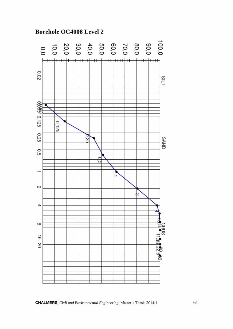
CHALMERS, Civil and Environmental Engineering, Master’s Thesis 2014:1 61
Borehole OC4008 Level 2
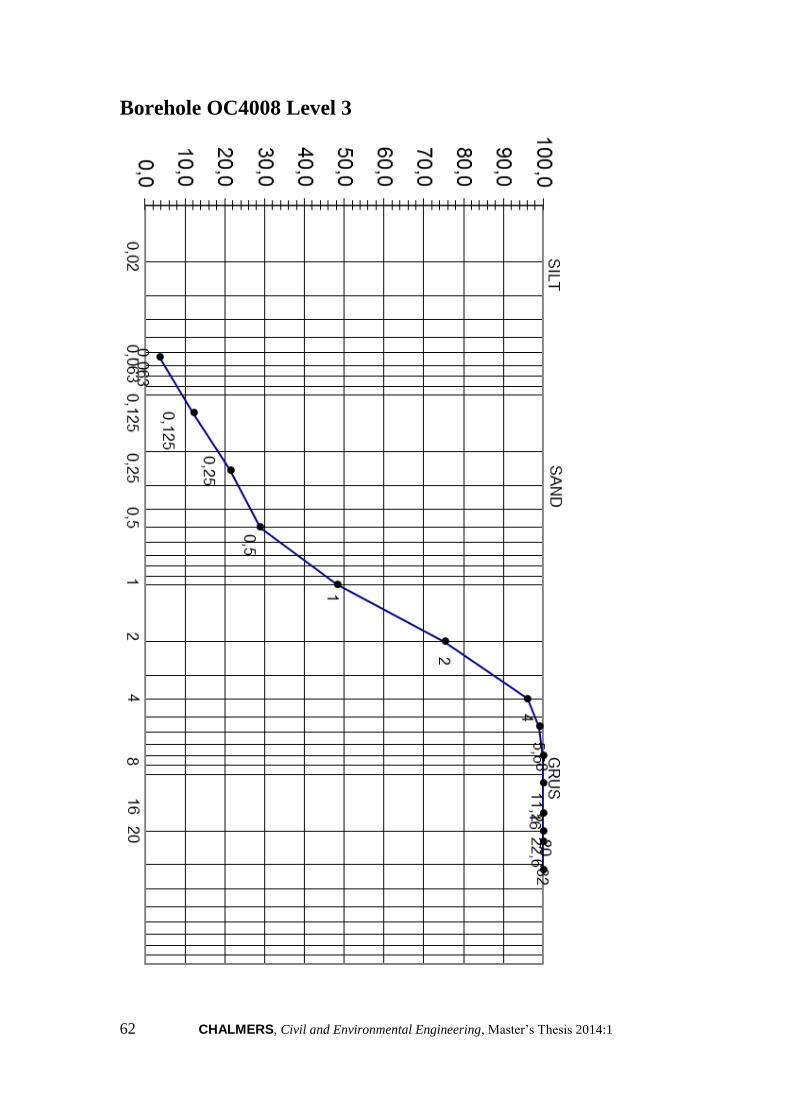
62 CHALMERS, Civil and Environmental Engineering, Master’s Thesis 2014:1
Borehole OC4008 Level 3

CHALMERS, Civil and Environmental Engineering, Master’s Thesis 2014:1 63
Borehole OC4009 Level 1

64 CHALMERS, Civil and Environmental Engineering, Master’s Thesis 2014:1
Borehole OC4009 Level 2

CHALMERS, Civil and Environmental Engineering, Master’s Thesis 2014:1 65
Borehole OC4010 Level 1

66 CHALMERS, Civil and Environmental Engineering, Master’s Thesis 2014:1
Borehole OC4011 Level 1

CHALMERS, Civil and Environmental Engineering, Master’s Thesis 2014:1 67
Borehole OC4011 Level 2

68 CHALMERS, Civil and Environmental Engineering, Master’s Thesis 2014:1
Borehole OC4012 Level 1

CHALMERS, Civil and Environmental Engineering, Master’s Thesis 2014:1 69
Appendix 2. Korsvägen
Borehole KK5040 Level 1

70 CHALMERS, Civil and Environmental Engineering, Master’s Thesis 2014:1
Borehole KK5040 Level 2

CHALMERS, Civil and Environmental Engineering, Master’s Thesis 2014:1 71
Borehole KK5040 Level 3

72 CHALMERS, Civil and Environmental Engineering, Master’s Thesis 2014:1
Borehole KK5038 Level 1

CHALMERS, Civil and Environmental Engineering, Master’s Thesis 2014:1 73
Borehole KK5038 Level 2
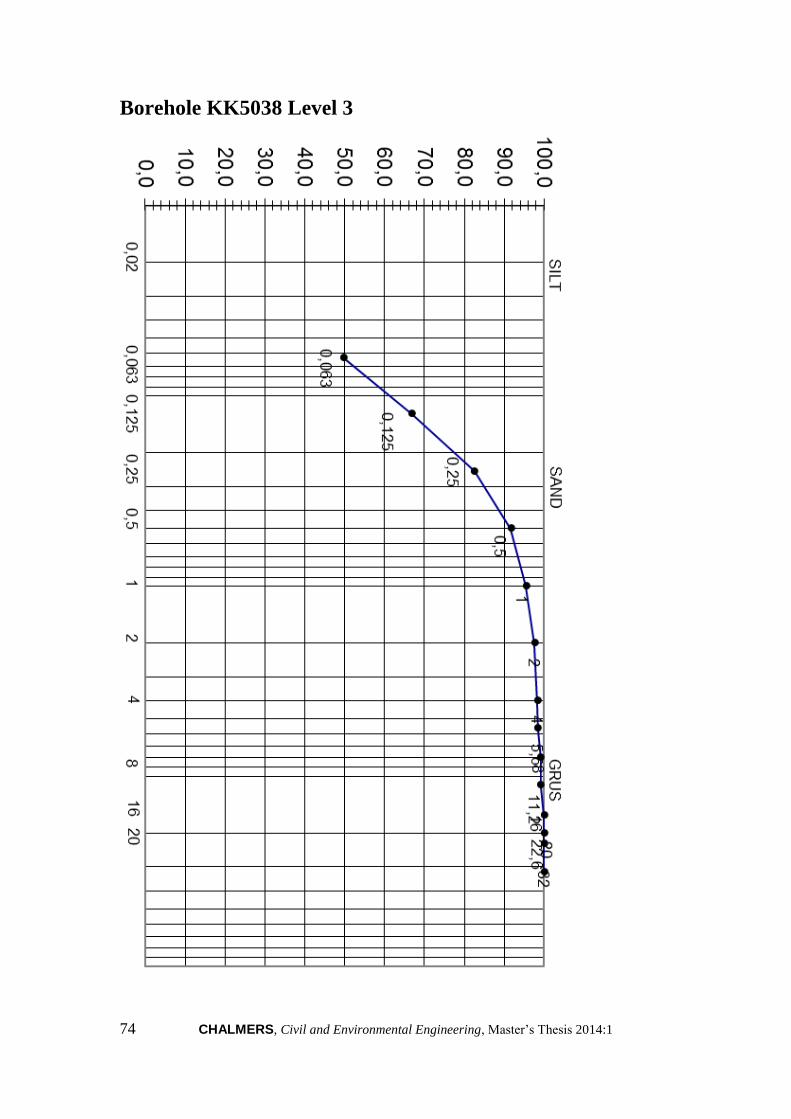
74 CHALMERS, Civil and Environmental Engineering, Master’s Thesis 2014:1
Borehole KK5038 Level 3

CHALMERS, Civil and Environmental Engineering, Master’s Thesis 2014:1 75
Borehole KK5038 Level 4

76 CHALMERS, Civil and Environmental Engineering, Master’s Thesis 2014:1
Appendix 3. Variation of hydraulic conductivity
based on degree of compaction
Very
Loose Loose Medium Compact
Very
Compact
Borehole KKC1 KKC2 KKC3 KKC4 KKC5 KKCexp
Skansen
OC4008-1 2,66E-06 2,25E-07 1,37E-07 7,43E-08 3,41E-08 1,62E-06
OC4008-2 3,37E-05 5,77E-06 4,28E-06 3,05E-06 2,07E-06 -
OC4008-3 1,91E-05 2,35E-06 1,60E-06 1,02E-06 5,99E-07 -
OC4009-1 4,24E-04 1,52E-04 1,31E-04 1,12E-04 9,49E-05 1,20E-04
OC4009-2 3,40E-04 1,09E-04 9,22E-05 7,71E-05 6,36E-05 1,13E-04
OC4010 1,82E-04 6,16E-05 5,26E-05 4,45E-05 3,72E-05 5,87E-05
OC4011-1 1,34E-04 5,07E-05 4,42E-05 3,82E-05 3,27E-05 -
OC4011-2 1,01E-04 3,49E-05 2,99E-05 2,54E-05 2,13E-05 3,23E-05
OC4012 1,04E-04 3,67E-05 3,16E-05 2,70E-05 2,28E-05 3,11E-05
Korsvägen
KK5040-1 1,13E-06 8,30E-08 4,82E-08 2,45E-08 1,01E-08 2,25E-07
KK5040-2 2,35E-05 6,55E-06 5,39E-06 4,37E-06 3,48E-06 4,34E-06
KK5040-3 7,51E-07 1,19E-07 8,65E-08 6,03E-08 3,97E-08 8,04E-08
KK5038-1 1,76E-05 4,59E-06 3,73E-06 2,98E-06 2,33E-06 3,70E-06
KK5038-2 5,46E-07 5,95E-08 3,91E-08 2,38E-08 1,30E-08 2,74E-07

CHALMERS, Civil and Environmental Engineering, Master’s Thesis 2014:1 77
1,00E-08
1,00E-07
1,00E-06
1,00E-05
1,00E-04
1,00E-03
1,00E-02
1,00E-01
1,00E+00
Very loose
Loose
Medium
Compact
Very compact
Experimental

78 CHALMERS, Civil and Environmental Engineering, Master’s Thesis 2014:1
Appendix 4. Graph of different porosities based on
degree of compaction and experimental porosity
0,00
0,05
0,10
0,15
0,20
0,25
0,30
0,35
0,40
0,45
0,50
Very loose
Loose
Medium
Compact
Very compact
Experimental

CHALMERS, Civil and Environmental Engineering, Master’s Thesis 2014:1 79
Appendix 5. ANOVA single factor analysis
Input data for ANOVA analysis
Skansen Lejonet KKC1 KKC2 KH KG
OC4007-1 2,7E-06 1,6E-06 4,6E-05 2,2E-05
OC4007-2 3,4E-05 8,8E-05 7,3E-05
OC4007-3 1,9E-05 1,2E-04 7,5E-05
OC4008-1 1,3E-04 1,2E-04 2,0E-04 2,8E-04
OC4008-2 9,2E-05 1,1E-04 2,0E-04 2,7E-04
OC4009 5,3E-05 5,9E-05 9,4E-05 1,3E-04
OC4010-1 4,4E-05 5,7E-05 8,3E-05
OC4010-2 3,0E-05 3,2E-05 5,0E-05 7,2E-05
OC4012 3,2E-05 3,1E-05 4,9E-05 7,0E-05
Korsvägen
KK5040-1 8,30E-08 2,3E-07 2,9E-05 1,3E-05
KK5040-2 4,4E-06 4,3E-06 1,9E-05 2,3E-05
KK5040-3 6,0E-08 8,0E-08 2,4E-06 1,9E-06
KK5038-1 3,0E-06 3,7E-06 1,6E-05 1,9E-05
KK5038-2 2,4E-08 2,7E-07 4,6E-06 2,7E-06
Skansen Lejonet Logarithmic values
OC4007-1 -5,5751184 -5,7895068 -4,3379855 -4,6548364
OC4007-2 -4,4723701 -4,0576281 -4,1346459
OC4007-3 -4,7189666 -3,9366666 -4,1271295
OC4008-1 -3,8827287 -3,9207195 -3,7087799 -3,5494819
OC4008-2 -4,0352691 -3,9467833 -3,7087799 -3,5716491
OC4009 -4,2790143 -4,2313392 -4,0281816 -3,8785834
OC4010-1 -4,3545777 -4,2464706 -4,0827968
OC4010-2 -4,5243288 -4,4910903 -4,2975788 -4,1445408
OC4012 -4,5003129 -4,5070089 -4,3108399 -4,1531684
Korsvägen
KK5040-1 -7,0809219 -6,6478103 -4,5387266 -4,9000584
KK5040-2 -5,3595186 -5,3627886 -4,7325467 -4,6372888
KK5040-3 -7,2196827 -7,0945944 -5,6259946 -5,7298486
KK5038-1 -5,5257837 -5,4321346 -4,7909234 -4,7179252
KK5038-2 -7,623423 -6,5616697 -5,3346066 -5,5670284
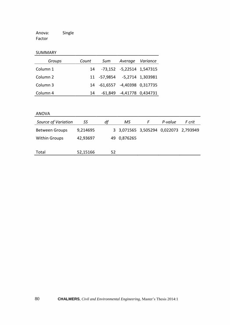
80 CHALMERS, Civil and Environmental Engineering, Master’s Thesis 2014:1
Anova: Single Factor
SUMMARY
Groups Count Sum Average Variance
Column 1 14 -73,152 -5,22514 1,547315
Column 2 11 -57,9854 -5,2714 1,303981
Column 3 14 -61,6557 -4,40398 0,317735
Column 4 14 -61,849 -4,41778 0,434731
ANOVA
Source of Variation SS df MS F P-value F crit
Between Groups 9,214695 3 3,071565 3,505294 0,022073 2,793949
Within Groups 42,93697 49 0,876265
Total 52,15166 52