estimation and optimization of flank wear an d tool ... · factor affecting workpiece surface...

* Corresponding author Tel.: (+213) 773996958; Fax: (+213) 37 21 58 50 E-mail: [email protected] (L. Bouzid) © 2018 Growing Science Ltd. All rights reserved. doi: 10.5267/j.ijiec.2017.8.002

International Journal of Industrial Engineering Computations 9 (2018) 349–368

Contents lists available at GrowingScience

International Journal of Industrial Engineering Computations

homepage: www.GrowingScience.com/ijiec

Estimation and optimization of flank wear and tool lifespan in finish turning of AISI 304 stainless steel using desirability function approach

Lakhdar Bouzidab*, Sofiane Berkania, Mohamed Athmane Yallesea, Frençois Girardinc and Tarek Mabroukid

aMechanical Engineering Department, Mechanics and Structures Research Laboratory (LMS), May 8th 1945 University, P.O. Box 401, Guelma 24000, Algeria bUniversity of Larbi Ben M’Hidi, Oum el Bouaghi, Algeria cLaboratoire Vibrations Acoustique, INSA-Lyon, 25 bis avenue Jean Capelle, F-69621 Villeurbanne Cedex, France dUniversity of Tunis El Manar, ENIT, Tunis, Tunisia C H R O N I C L E A B S T R A C T

Article history: Received May 1 2017 Received in Revised Format July 1 2017 Accepted August 11 2017 Available online August 11 2017

The wear of cutting tools remains a major obstacle. The effects of wear are not only antagonistic at the lifespan and productivity, but also harmful with the surface quality. The present work deals with some machinability studies on flank wear, surface roughness, and lifespan in finish turning of AISI 304 stainless steel using multilayer Ti(C,N)/Al2O3/TiN coated carbide inserts. The machining experiments are conducted based on the response surface methodology (RSM). Combined effects of three cutting parameters, namely cutting speed, feed rate and cutting time on the two performance outputs (i.e. VB and Ra), and combined effects of two cutting parameters, namely cutting speed and feed rate on lifespan (T), are explored employing the analysis of variance (ANOVA). The relationship between the variables and the technological parameters is determined using a quadratic regression model and optimal cutting conditions for each performance level are established through desirability function approach (DFA) optimization. The results show that the flank wear is influenced principally by the cutting time and in the second level by the cutting speed. In addition, it is indicated that the cutting time is the dominant factor affecting workpiece surface roughness followed by feed rate, while lifespan is influenced by cutting speed. The optimum level of input parameters for composite desirability was found Vc1-f1-t1 for VB, Ra and Vc1-f1 for T, with a maximum percentage of error 6.38%.

© 2018 Growing Science Ltd. All rights reserved

Keywords: Flank wear Surface roughness Lifespan Modeling DFA Optimization

1. Introduction

The tool wear, especially the flank wear, is one of the most important aspects that affect lifespan and product quality in machining. It is a major form of tool wear in metal cutting, which adversely affects the dimensional accuracy and product quality, is the main hurdle in the wide implementation of coated carbide tools to machining of stainless steel in the industry. Practically the lifespan is evaluated by the measure of the flank wear. If it increases quickly, the lifespan becomes very short and vice versa. In finish turning, tool life is measured by the machining time taken by the same insert until the flank wear reaches its allowable limit of 0.3 mm. Wear is an important technological parameter of control in the machining process. It is the background for the evaluation of the tool life and surface quality (Yallese et

350

al., 2008; Uvaraja & Natarajan, 2012; Çaydas, 2010). Therefore, development of a reliable flank wear progression model will be extremely valuable. Significant efforts have been devoted by several researchers in understanding and modeling the tool wear progression, wear mechanisms, tool lifespan and surface quality in metal cutting. In recent years, a significant emphasis has been placed in the development of predictive models in metal cutting. Analytical models are easy to implement and can give much more insight about the physical behavior in metal cutting. Kramer (1986) developed a model for prediction of the wear rates of coated tools in high-speed machining of steel. The abrasive wear and the chemical dissolution were considered as dominant wear mechanisms. Singh and Rao (2010) developed flank wear prediction model of ceramic inserts in hard turning. Flank wear rate was modeled considering abrasion, adhesion, and diffusion as dominant wear mechanisms. Normal load/force incurred on the flank face was modeled using experimental results. However, increase in the normal load with the progress in flank wear was not considered in the model. It is widely reported that cutting forces influence more with the progress in flank wear, which appeared as one of the most promising techniques for monitoring tool wear. Singh and Vajpayee (1980) developed a flank wear model considering abrasion as the dominant wear mechanism. Yallese et al. (2009) have shown that for the 100Cr6 steel, the machined surface roughness is a function of the local damage form and the wear profile of a CBN tool. When augmenting cutting speed tool wear increases and leads directly to the degradation of the surface quality. In spite of the evolution of flank wear up to the allowable limit VB =0.3 mm, arithmetic roughness Ra did not exceed 0.55 µm. A relation between VB and Ra in the form Ra = k.eβ(VB) is proposed. Coefficients k and β vary within the ranges of 0.204–0.258 and 1.67–2.90, respectively. It permits the follow-up of the tool wear.

A common problem in product or process design is the selection of design variable setting which meets a required specification of quality characteristics. For this purpose, among global approximation approaches, the response surface methodology (RSM) has recently attracted the most attention since it has performed well in comparison to other approaches (Garcia et al., 1981; Smith, 1973). RSM consists of the following three steps: (1) data gathering, (2) modeling, and (3) optimization (Aouici et al., 2014). Neşeli et al. (2011) applied response surface methodology (RSM) to optimize the effect of tool geometry parameters on surface roughness in hard turning of AISI 1040 with P25 tool. Yallese et al. (2009) found that a cutting speed of 120 m/min is an optimal value for machining X200Cr12 using CBN7020. In an original work carried out by Çaydaş (2009), the effects of the cutting speed, feed rate, depth of cut, workpiece hardness, and cutting tool type on surface roughness, tool flank wear, and maximum tool–chip interface temperature during an orthogonal hard turning of hardened/tempered AISI 4340 steels were investigated. Dureja et al. (2009) applied the response surface methodology (RSM) to investigate the effect of cutting parameters on flank wear and surface roughness in hard turning of AISI H11 steel with a coated-mixed ceramic tool. The study indicated that the flank wear is influenced principally by feed rate, depth of cut and workpiece hardness. When turning hardened 100Cr6, Banga and Abrão (2003) found that cutting speed is the most factor influencing tool lifespan. These authors have shown that PCBN cutting tools provide longer tool lifespan than both mixed and composite ceramics. A model built to evaluate the machinability of Hadfield steel using RMS and ANOVA techniques was presented by (Horng et al., 2008). The study revealed that the flank wear is influenced by the cutting speed while the interaction effect of the feed rate with the nose radius and the corner radius of the tool have statistical significance on obtained surface roughness. The current study investigates the influence of cutting parameters (cutting speed, feed rate and cutting time, with a constant cutting depth ap = 0.15 mm) in relation to flank wear (VB), lifespan (T) and surface roughness (Ra) on machinability. The processing conditions are turning of stainless steel (AISI 304) with CVD coated carbide tools using both response surface methodology (RSM) and ANOVA. This latter is a computational technique that enables the estimation of the relative contributions of each of the control factors to the overall measured response. In this work, only the significant parameters will be used to develop mathematical models using response surface methodology. The latter is a collection of mathematical and statistical techniques that are useful for the modeling and analysis of

L. Bouzid et al. / International Journal of Industrial Engineering Computations 9 (2018) 351

problems in which response of interest is influenced by several variables and the objective is to optimize the response.

2. Experimental procedures

2.1. Material

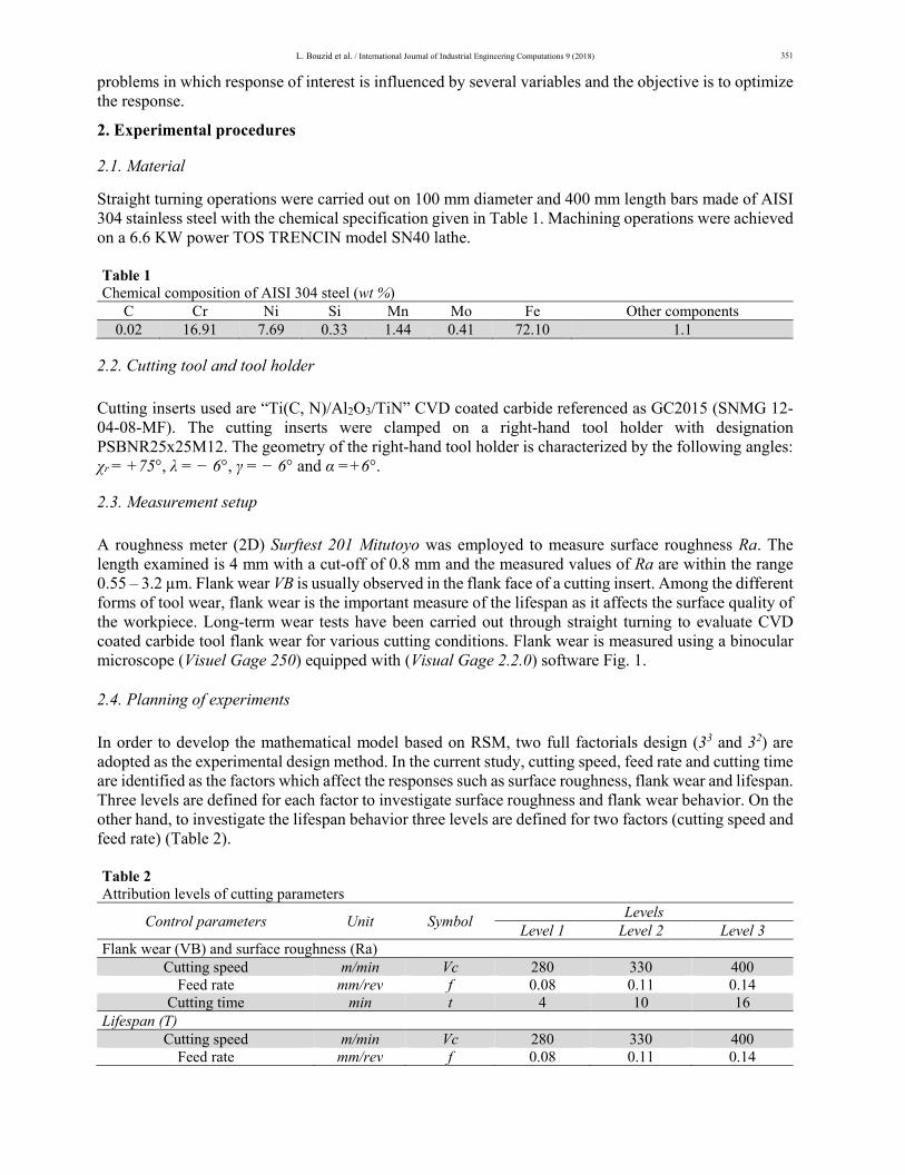
Straight turning operations were carried out on 100 mm diameter and 400 mm length bars made of AISI 304 stainless steel with the chemical specification given in Table 1. Machining operations were achieved on a 6.6 KW power TOS TRENCIN model SN40 lathe. Table 1 Chemical composition of AISI 304 steel (wt %)

C Cr Ni Si Mn Mo Fe Other components 0.02 16.91 7.69 0.33 1.44 0.41 72.10 1.1

2.2. Cutting tool and tool holder

Cutting inserts used are “Ti(C, N)/Al2O3/TiN” CVD coated carbide referenced as GC2015 (SNMG 12-04-08-MF). The cutting inserts were clamped on a right-hand tool holder with designation PSBNR25x25M12. The geometry of the right-hand tool holder is characterized by the following angles: χr = +75°, λ = − 6°, γ = − 6° and α =+6°.

2.3. Measurement setup

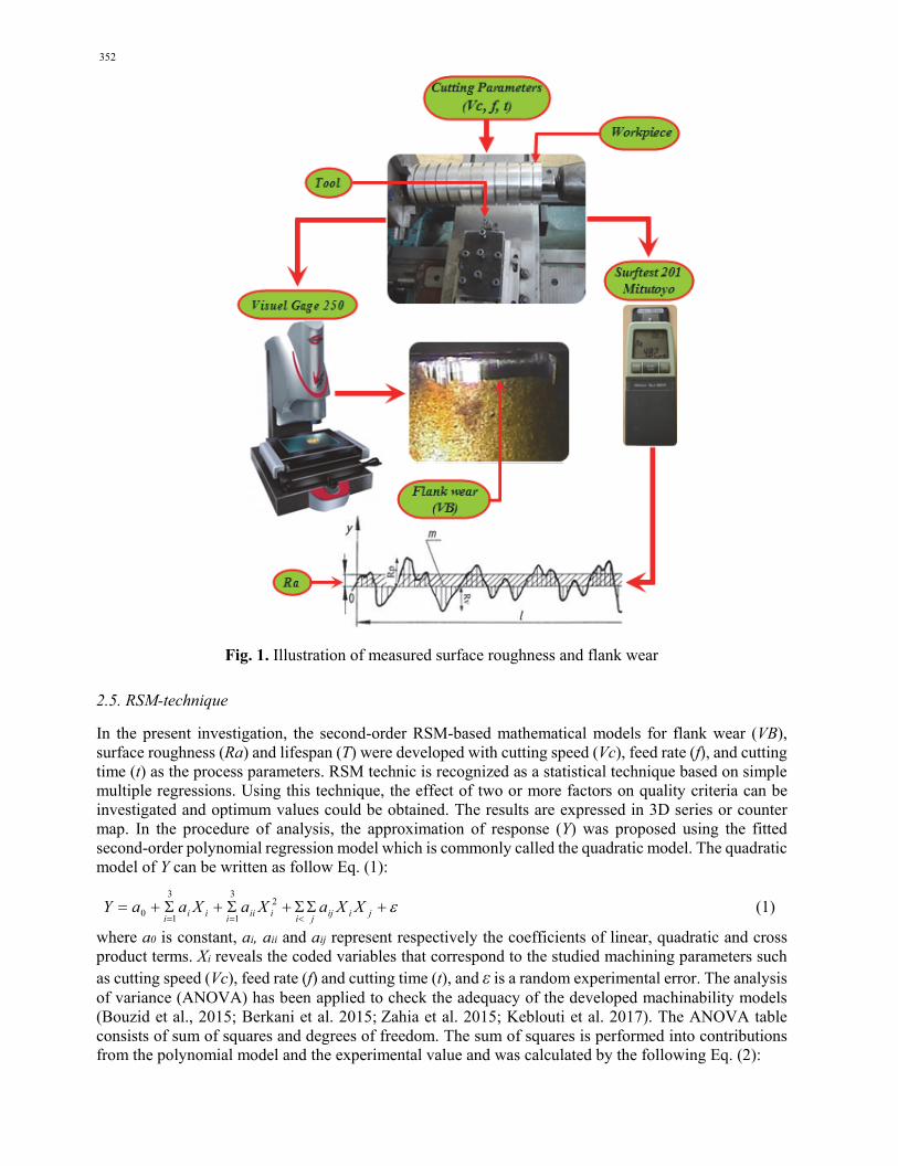
A roughness meter (2D) Surftest 201 Mitutoyo was employed to measure surface roughness Ra. The length examined is 4 mm with a cut-off of 0.8 mm and the measured values of Ra are within the range 0.55 – 3.2 µm. Flank wear VB is usually observed in the flank face of a cutting insert. Among the different forms of tool wear, flank wear is the important measure of the lifespan as it affects the surface quality of the workpiece. Long-term wear tests have been carried out through straight turning to evaluate CVD coated carbide tool flank wear for various cutting conditions. Flank wear is measured using a binocular microscope (Visuel Gage 250) equipped with (Visual Gage 2.2.0) software Fig. 1.

2.4. Planning of experiments

In order to develop the mathematical model based on RSM, two full factorials design (33 and 32) are adopted as the experimental design method. In the current study, cutting speed, feed rate and cutting time are identified as the factors which affect the responses such as surface roughness, flank wear and lifespan. Three levels are defined for each factor to investigate surface roughness and flank wear behavior. On the other hand, to investigate the lifespan behavior three levels are defined for two factors (cutting speed and feed rate) (Table 2). Table 2 Attribution levels of cutting parameters

Control parameters Unit Symbol Levels

Level 1 Level 2 Level 3 Flank wear (VB) and surface roughness (Ra)

Cutting speed m/min Vc 280 330 400 Feed rate mm/rev f 0.08 0.11 0.14

Cutting time min t 4 10 16 Lifespan (T)

Cutting speed m/min Vc 280 330 400 Feed rate mm/rev f 0.08 0.11 0.14

352

Fig. 1. Illustration of measured surface roughness and flank wear

2.5. RSM-technique

In the present investigation, the second-order RSM-based mathematical models for flank wear (VB), surface roughness (Ra) and lifespan (T) were developed with cutting speed (Vc), feed rate (f), and cutting time (t) as the process parameters. RSM technic is recognized as a statistical technique based on simple multiple regressions. Using this technique, the effect of two or more factors on quality criteria can be investigated and optimum values could be obtained. The results are expressed in 3D series or counter map. In the procedure of analysis, the approximation of response (Y) was proposed using the fitted second-order polynomial regression model which is commonly called the quadratic model. The quadratic model of Y can be written as follow Eq. (1):

jiij

jiiii

iii

iXXaXaXaaY 2

3

1

3

10 (1)

where a0 is constant, ai, aii and aij represent respectively the coefficients of linear, quadratic and cross product terms. Xi reveals the coded variables that correspond to the studied machining parameters such as cutting speed (Vc), feed rate (f) and cutting time (t), and ε is a random experimental error. The analysis of variance (ANOVA) has been applied to check the adequacy of the developed machinability models (Bouzid et al., 2015; Berkani et al. 2015; Zahia et al. 2015; Keblouti et al. 2017). The ANOVA table consists of sum of squares and degrees of freedom. The sum of squares is performed into contributions from the polynomial model and the experimental value and was calculated by the following Eq. (2):


2

1

)( yyN

NSS

nfN

ii

nff

(2)

The mean square is the ratio of sum of squares to degrees of freedom was calculated by the following Eq. (3):

= fi

i

SSMs

df (3)

The F-value is the ratio of mean square of regression model to the mean square of the experimental error was calculated by the following Eq. (4):

e

ii Ms

MsF (4)

This analysis was out for a 5 % significance level, i.e., for a 95 % confidence level. The last column of the tables shows the percentage of each factor contribution (Cont. %) on the total variation, then indicating the degree of influence on the result, was calculated by the following Eq. (5):

100.% T

f

SS

SSCont

(5)

3. Results and discussion

Table 3 and Table 4 show all the values of the response factors: flank wear (VB), surface roughness (Ra) and lifespan (T), and were made with the objective of analysing the influence of the cutting speed (Vc), feed rate (f), and cutting time (t) on the total variance of the results. The surface roughness was obtained in the range of 0.55–3.2 μm, flank wear and lifespan were obtained in the range of 0.025-0.51 mm, and 10-44 min, respectively.

Table 3 Experimental results for surface roughness and flank wear

Run Factors Responses

Vc, m/min f, mm/rev t, min Ra, µm VB, mm 1 280 0.08 4 0.56 0.025 2 280 0.08 10 0.61 0.050 3 280 0.08 16 0.74 0.100 4 280 0.11 4 0.81 0.030 5 280 0.11 10 1.17 0.074 6 280 0.11 16 1.25 0.110 7 280 0.14 4 1.32 0.045 8 280 0.14 10 1.34 0.069 9 280 0.14 16 1.35 0.110

10 330 0.08 4 0.55 0.040 11 330 0.08 10 0.62 0.115 12 330 0.08 16 0.80 0.190 13 330 0.11 4 0.79 0.060 14 330 0.11 10 1.21 0.135 15 330 0.11 16 1.60 0.170 16 330 0.14 4 1.31 0.06 17 330 0.14 10 1.47 0.185 18 330 0.14 16 1.92 0.350 19 400 0.08 4 0.80 0.050 20 400 0.08 10 1.24 0.200 21 400 0.08 16 1.99 0.410 22 400 0.11 4 0.87 0.065 23 400 0.11 10 1.55 0.290 24 400 0.11 16 2.95 0.460 25 400 0.14 4 1.16 0.070 26 400 0.14 10 1.70 0.300 27 400 0.14 16 3.20 0.510

354

Table 4 Experimental results for lifespan

Run Factors Response

Vc, m/min f, mm/rev T, min 1 280 0.08 44 2 280 0.11 42 3 280 0.14 39 4 330 0.08 27 5 330 0.11 20 6 330 0.14 15 7 400 0.08 15 8 400 0.11 11 9 400 0.14 10

3.1. ANOVA results

Table 5 shows the results of ANOVA analysis for flank wear surface roughness and lifespan. In addition, the same Table 5 shows the degrees of freedom, sum of square, mean of square, F-value and P-value. Table 5 ANOVA for response surface quadratic models

Source df SS Ms F P Cont,% Remarques a) Flank wear (VB)

Model 9 0.49 0.05 65.46 < 0.0001 97.2 Significant Vc 1 0.17 0.17 203.66 < 0.0001 33.6 Significant f 1 0.02 0.02 18.91 0.0004 3.12 Significant t 1 0.23 0.23 279.92 < 0.0001 46.18 Significant

Vc×f 1 0.00 0.00 2.50 0.1326 0.41 Not Significant Vc×t 1 0.08 0.08 98.26 < 0.0001 16.21 Significant f×t 1 0.00 0.00 4.44 0.0503 0.73 SignificantVc² 1 0.00 0.00 0.10 0.7539 0.02 Not Significant f² 1 0.00 0.00 0.19 0.6723 0.03 Not Significant t² 1 0.00 0.00 0.01 0.9294 0 Not Significant

Residual 17 0.01 0.00

Total 26 0.50

b) Surface roughness (Ra) Model 9 10.51 1.17 31.75 < 0.0001 94.34 Significant

Vc 1 2.21 2.21 60.14 < 0.0001 19.84 Significant f 1 2.59 2.59 70.52 < 0.0001 23.25 Significant t 1 3.56 3.56 96.88 < 0.0001 31.96 Significant

Vc×f 1 1.7.10-3 1.7.10-3 0.046 0.8319 0.02 Not SignificantVc×t 1 1.91 1.91 51.85 < 0.0001 17.15 Significant f×t 1 0.094 0.094 2.55 0.129 0.84 Not Significant Vc² 1 0.17 0.17 4.55 0.0479 1.53 Significant f² 1 0.055 0.055 1.49 0.2389 0.49 Not Significant t² 1 0.086 0.086 2.33 0.1455 0.77 Not Significant

Residual 17 0.63 0.037

Total 26 11.14

c) Lifespan (T) Model 5 1477.93 295.59 50.30 0.0043 98.82 Significant

Vc 1 1320.17 1320.17 224.67 0.0006 88.27 Significant f 1 79.83 79.83 13.59 0.0346 5.34 Significant

Vc×f 1 0.15 0.15 0.03 0.8833 0.01 Not Significant Vc² 1 147.89 147.89 25.17 0.0153 9.89 Significant f² 1 0.89 0.89 0.15 0.7233 0.06 Not Significant

Residual 3 17.63 5.88

Total 8 1495.56

The ration of contribution of different factors and their interactions were also presented. The main purpose was to analyse the influence of cutting speed (Vc), feed rate (f), and cutting time (t) on the total variance of the results. From the analysis of Table 5, it can be apparent seen that the cutting time (t), cutting speed (Vc), interactions (Vc×t, f×t) and feed rate (f) all have significant effect on the flank wear


(VB). But, the effect of cutting time is the most significant factor associated for flank wear with 46.18 %. The next largest factor influencing VB is the cutting speed. Its contribution is 33.60 % to the model. The interaction (Vc×t) were less significant, while (Vc×f) interaction and productions (Vc², f², t²) were found to be negligible. However, the value of “P” in Table 5 for surface roughness (Ra) model is less than 0.05 which indicates that the model is significant, which is desirable as it indicates that the terms in the model have a significant effect on the response. In the same manner, the main effect of cutting time (t), feed rate factor (f), cutting speed (Vc), the interaction of cutting speed and cutting time (Vc×t), and the product (Vc²) are significant model terms. It can be seen that the cutting time (t) is the most important factor affecting Ra. Its contribution is 31.96 %. The second important factor affecting Ra is the feed rate, because its increase generates helicoid furrows, the result of tool shape and helicoid movement tool-workpiece. These furrows are deeper and broader as the feed rate increases. Its contribution is 23.25%. The next factors influencing Ra are the cutting speed, the interaction (Vc×t) and the product (Vc²). Other model terms can be said to be not significant. Finality, it can be apparently seen in Table 5 that the cutting speed factor (Cont. ≈ 88 %), the feed rate factor (Cont. ≈ 5 %) and the product Vc² (Cont. ≈ 9.9 %) have statistical significance on the lifespan (T), especially the cutting speed.

3.2. Influential factors

To better view the results of the analysis of variance, a Pareto graph is built (Fig. 2 a, b, and c). This figure ranks the cutting parameters and their interactions of their growing influence on the flank wear (VB), surface roughness (Ra) and lifespan (T). Effects are standardized (F-value) for a better comparison. If the (F-value) values are greater than (F-table = 4.45) for VB and Ra; and greater than (F-table = 10.13) for lifespan, the effects are significant. By cons, if the values of F-value are less than (4.45; 10.13) the effects are not significant. The confidence interval chosen is 95 %.

(a) (b)

(c)

Fig. 2. Pareto graphs of: a) flank wear, b) surface roughness and c) lifespan

356

3.3. Regression equations

The relationship between the inputs (cutting speed, feed rate and cutting time) and outputs (VB, Ra and T) was modelled by quadratic regression equations. The different quadratic models obtained from statistical analysis can be used to predict the flank wear, surface roughness and lifespan according to the studied factors. The models and its determination coefficients obtained for different cutting phenomena are presented in Eqs. (6-8) respectively to (flank wear, surface roughness and lifespan).

= × ×

× ×

-6 2

-5 2

VB 0.65 - 0.0021Vc - 3.68f - 0.069t + 1.074.10 Vc + 0.0072 Vc f + 0.00022Vc t

+ 5.61f f + 0.097 f t +2.93.10 t

(6)

R²= 97.20%

= × ×

×

-5 2 -3

2 2

Ra 5.68- 0.037 Vc + 33.37 f - 0.421 t + 4.79.10 Vc - 6.6.10 Vc f + 0.0011Vc t

- 106.173 f + 0.49f t +0.0033 t

(7)

R² = 94.39% 22 740,741f+ fVc 0,11 +0,0024Vc + f 321,22 - 1,94Vc - 413,26T (8)

R² = 98.82% In order to reduce the models, only the significant parameters will be conserved.

× ×-4 -4V B = 0.19 - 6.59.10 V c - 0.011f - 0.069t + 2.27.10 V c t + 0.097222f t (9)

R²= 96.73% Ra = 6.35 – 0.037 Vc + 12.703 f – 0.3 t + 1.102.10-3 Vc×t + 4.79.10-5 Vc2 (10)

R²= 92.27% T = 400.77 – 1.92 Vc - 122.22 f – 2.47.10-3 Vc2 (11)

R²= 98.75%

3.4. Models validation

3.4.1. Graphical Validation

The above models can be used to predict flank wear, surface roughness and lifespan at the particular design points. The differences between measured and predicted responses are illustrated in Figs. (3-5). These figures indicate that the quadratic models are capable to representing the system under the given experimental domain.

Fig. 3. Comparison between measured and predicted values for flank wear

0

0.1

0.2

0.3

0.4

0.5

0.6

0 5 10 15 20 25 30

VB

, mm

Experimental Run

VB‐ meas VB‐pred


Fig. 4. Comparison between measured and predicted values for surface roughness

Fig. 5. Comparison between measured and predicted values for lifespan

0

0.5

1

1.5

2

2.5

3

3.5

0 5 10 15 20 25 30

Ra,

µm

Experimental Run

Ra‐meas Ra‐pred

0

5

10

15

20

25

30

35

40

45

50

0 1 2 3 4 5 6 7 8 9

T, m

in

Experimental Run

T‐meas T‐pred

Residuals

Per

cent

-2.00 -1.00 0.00 1.00 2.00

1

5

10

20

30

50

70

80

90

95

99

b)

Residuals

Per

cent

-3.00 -2.00 -1.00 0.00 1.00 2.00 3.00

1

5

10

20

30

50

70

80

90

95

99

a)

358

Fig. 6. Normal probability plots of predicted response for: a) flank wear, b) surface roughness and c) lifespan

The Anderson–Darling test and normal probability plots of predicted response for: surface roughness, flank wear and tool lifespan respectively, are presented in Figs.6 (a, b, c). The data closely follows the straight line. The null hypothesis is that the data distribution law is normal and the alternative hypothesis is that it is non-normal. Using the P-value which is greater than alpha of 0.05 (level of significance), the null hypothesis cannot be rejected (i.e., the data don’t follow a normal distribution). It implies that the models proposed are adequate.

3.4.2. Mathematical validation

The analysis of variance (ANOVA) was used to check the adequacy of developed models for a given confidence interval. The ANOVA table consists of sum of squares and degrees of freedom. In order to perform an ANOVA, the sum of squares is usually completed into contributions from regression model and residual error. As for this technique, if the calculated value of F-ratio of model is more than the standard tabulated value of table (F-table) for a given confidence interval, then the model is adequate within the confidence limit (Meddour et al., 2015; Muthukrishnan & Davim, 2009; Elbah et al., 2013). The adequacy of developed mathematical models is presented in Tables 6. The model accuracy (Δ) is commonly given by the following Eq.12 (Kaddeche et al., 2012):

n

i predi

prediti

y

yy

n 1 ,

,exp,100, (12)

where yi,expt is the measured value of response corresponding to i th trial, yi,pred is the predicted value of response corresponding to i th trial and n is the number of trials. Eqs. (9-11) are used to test the accuracy of the models using the experimental data. The prediction errors of these models are illustrated in Table 6 together with determination coefficients. It is concluded that the correlations are valid and can be used for predictions when turning AISI304 stainless steel. Table. 6 ANOVA analysis, percent prediction error of the experimental data and R2 values for VB, Ra and T

Responses

SS D. f Ms F-test F-table

P-value M R M R M R

VB 0.48 0.014 9 17 0.054 0.0008 65.45 2.49 < 0.0001 Ra 10.51 0.63 9 17 1.17 0.037 31.75 2.49 < 0.0001 T 1477.9 17.62 5 3 259.58 5.87 50.3 9.01 0.0043

M: model; R: residual Responses % Prediction error of the experimental data R2 (%) Values of models

VB 14.31 96.73 Ra 11.51 92.27 T 6.14 98.75

Residuals

Per

cent

-2.00 -1.00 0.00 1.00 2.00

1

5

10

20

30

50

70

80

90

95

99

c)


3.5. Responses surface analysis

3.5.1. Flank wear

Fig. 7 illustrates the evolution of the flank wear according to the cutting speed, cutting time and feed rate. It is found that tool wear increases with increasing effects of both cutting time and speed. It can be concluded that the cutting time exhibits maximum influence on flank wear. The maximum value of flank wear is found with height level of cutting time and cutting speed.

Fig. 7. Effect of cutting speed, feed rate and cutting time on flank wear

3.5.2. Workpiece surface roughness

The estimated response surface for the surface roughness in relation to the cutting parameters (Vc, f and t) presented in (Fig. 8.) shows that the cutting speed had a significant influence on machined surface roughness.

Fig. 8. Effect of cutting speed, feed rate and cutting time on surface roughness

0.08

0.10

0.11

0.13

0.14

280

310

340

370

400

0

0.1

0.2

0.3

0.4

0.5

0.6

VB

, mm

Vc, m/min f, mm/rev

d v alue

4

7

10

13

16

280

310

340

370

400

0

0.1

0.2

0.3

0.4

0.5

VB

, mm

Vc, m/min

t, min

d v alue

0.08

0.10

0.11

0.13

0.14

280

310

340

370

400

0

0.5

1

1.5

2

2.5

3

Ra

, µm

Vc, m/min f, mm/rev

d v alue

4

7

10

13

16

280

310

340

370

400

0

0.5

1

1.5

2

2.5

3

Ra

, µm

Vc, m/min t, min

360

A high values of surface roughness noted in small value of cutting speed that can be explained by the presence of built up edge (Fig. 9.) on the surface due to the high ductility of austenitic stainless steel. With the increasing of cutting speed the surface roughness values decrease until a minimum value reached beyond which they increase. The decrease in surface roughness when increasing of cutting speed to 340 m/min can be explained by the presence of micro-welds on machined surface due to high heat at cutting zone and the height of built-up-edge which lead to the breaking of BUE and carried away on the machined surface as seen in (Fig. 9). Further, increasing the cutting speed causes an increase in surface roughness because the cutting tool nose wear increases causing the poor surface finish (Ciftci, 2005). In the other hand, the roughness (Ra) tends to increase, considerably with increase in feed rate (f) and cutting time (t).

Fig. 9. Micro-Weld on machined surface and Built-Up Edge on cutting insert

3.5.3. Lifespan

The effect of feed rate (f) and cutting speed (Vc) on the tool life (T) is shown in Fig. 10. This figure displays that the value of tool life (T) decrease with the increase of cutting speed and feed rate. The decrease is approximately 77.27% of T.

Fig. 10. Effect of cutting speed and feed rate on tool lifespan

0.08 0.10

0.11 0.13

0.14

280

310

340

370

400

0

10

20

30

40

50

T, m

in

Vc, m/min

f, mm/rev


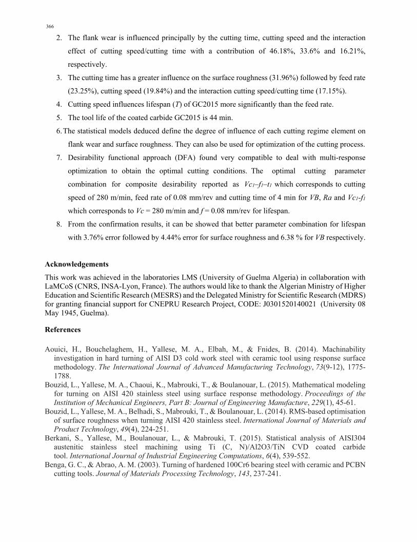
3.6. Micrographs for flank wear VB of the GC2015 tool

For the considered regime (Vc = 280 m/min, ap = 0.15 mm and f = 0.08 mm/rev), flank wear VB of the coated carbide tool GC2015 spreads regularly. Figure 11 shows the micrographs for VB of GC2015 insert, its lifetime is 44 min.

Fig. 11. Micrographs for VB of GC2015 at ap = 0.15 mm; f = 0.08 mm/rev and Vc = 280 m/min

4. Optimisation of machining performance using desirability function approach (DFA)

The desirability function approach to simultaneously optimizing multiple responses was originally proposed by Derringer and Suich. Essentially, the approach is to translate the functions to a common scale [0, 1], combine them using the geometric mean and optimize the overall metric. DFA continue to be a commonly preferred method because it can solve multi response optimization problem by converting it into single response optimization problem which enable to sort the computational work (Bouzid et al., 2014). The concept of desirability function involves the translation of the responses from its individual desirability to scale of composite desirability (overall desirability function). The DFA optimization process is used to perform through the following steps: Step 1: Define the independent input parameters of the experimental design and the desired responses

(yi) to be optimized.

Step 2: Adopt an experimental design plan and conduct experiments for the designed parameter

combinations.

Step 3: Calculate individual desirability (di ) for each response (yi) using desirability functions.

‐ Larger–the–Better: For a goal to find a maximum, the individual desirability is shown as follows:

0 if min

min if min maxmax min

1 if min

y yi iy yi idi y y yi i iy yi i

y yi i

(13)

‐ Smaller–the–Better: For a goal to find a minimum, the individual desirability is shown as follows:

VB = 0.025 mm, t = 4 min VB = 0.11 mm, t = 16 min VB = 0.18 mm, t = 20 min

VB = 0.26 mm, t = 30 min VB = 0.31 mm, t = 44 min

362

0 if min

max if min maxmax min

1 if min

y yi iy yi idi y y yi i iy yi i

y yi i

(14)

Step 4: Select the parameter combination that will maximize composite desirability (Dc), and determine the optimal parameter and its level combination based on the higher value of composite desirability (Dc).

1

,1

p PDc di

i

(15)

where (di) is the individual desirability of the response (i) and (P) is the number of response in the measure. The desirability ranges from zero to one. Step 5: The last step is performing ANOVA to indicate the most significant factor that affects the multiple performance characteristics.

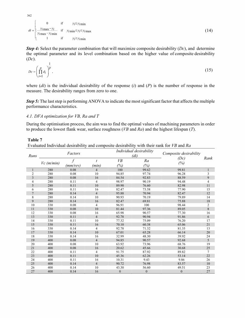
4.1. DFA optimization for VB, Ra and T

During the optimisation process, the aim was to find the optimal values of machining parameters in order to produce the lowest flank wear, surface roughness (VB and Ra) and the highest lifespan (T). Table 7 Evaluated Individual desirability and composite desirability with their rank for VB and Ra

Runs

Factors Individual desirability

(di) Composite desirability

(Dc) (%)

Rank Vc (m/min)

f (mm/rev)

t (min)

VB (%)

Ra (%)

1 280 0.08 4 100 99.62 99.81 1 2 280 0.08 10 94.85 97.74 96.28 3 3 280 0.08 16 84.54 92.83 88.59 9 4 280 0.11 4 98.97 90.19 94.48 4 5 280 0.11 10 89.90 76.60 82.98 11 6 280 0.11 16 82.47 73.58 77.90 15 7 280 0.14 4 95.88 70.94 82.47 12 8 280 0.14 10 90.93 70.19 79.89 14 9 280 0.14 16 82.47 69.81 75.88 18

10 330 0.08 4 96.91 100 98.44 2 11 330 0.08 10 81.44 97.36 89.05 8 12 330 0.08 16 65.98 90.57 77.30 16 13 330 0.11 4 92.78 90.94 91.86 6 14 330 0.11 10 77.32 75.09 76.20 17 15 330 0.11 16 70.10 60.38 65.06 21 16 330 0.14 4 92.78 71.32 81.35 1317 330 0.14 10 67.01 65.28 66.14 20 18 330 0.14 16 32.99 48.30 39.92 24 19 400 0.08 4 94.85 90.57 92.68 5 20 400 0.08 10 63.92 73.96 68.76 19 21 400 0.08 16 20.62 45.66 30.68 25 22 400 0.11 4 91.75 87.92 89.82 7 23 400 0.11 10 45.36 62.26 53.14 22 24 400 0.11 16 10.31 9.43 9.86 26 25 400 0.14 4 90.72 76.98 83.57 10 26 400 0.14 10 43.30 56.60 49.51 23 27 400 0.14 16 0 0 0 27


At first the evaluation of individual desirability (di) has been carried out for each response (yi) based on function Smaller–the–Better given in Eq. (13), which is used for minimization and Larger–the–Better as given in Eq. (14) used for maximization of response. Then, individual desirability (di ) of each response characteristics are fluxed into the composite desirability (Dc) by using Eq. (15). Tables 7 and 8 show the evaluated individual desirability and composite desirability values for each of the experimental trials.

Table 8 Evaluated Individual desirability and composite desirability with their rank for lifespan T

Runs Factors Composite desirability

(Dc) (%)

Rank Vc m/min

f mm/rev

1 280 0.08 100 1 2 280 0.11 94.12 2 3 280 0.14 85.29 3 4 330 0.08 50 4 5 330 0.11 29.41 5 6 330 0.14 14.71 6 7 400 0.08 14.71 7 8 400 0.11 2.94 8 9 400 0.14 0.00 9

The composite desirability (Dc) has computed and the ranks are assigned to them in ascending order and it is found that the higher composite desirability value (Dc = 99.81% for VB and Ra; Dc = 100% for T) obtained for the 1st trial of the experiment and its corresponding cutting combination may be regarded as optimal combination which emphasize on being closer to the experimental results. To ensure the optimal combination of levels for various factors, Table 9 shows the response mean of average composite desirability function for each level and total mean of composite desirability is also evaluated. The maximum mean of composite desirability value of each level of the factors gives the optimum cutting combination which is (Vc1–f1–t1) for VB and Ra, and (Vc1-f1) for T.

Table 9 Response table for Composite desirability (Dc) Flank wear (VB) and Surface roughness (Ra)

Levels Average composite desirability

Vc, % f, % t, % 1 88.72 80.16 92.67 2 75.62 72.20 73.04 3 52.06 64.04 50.70

Max-Min 36.66 16.12 41.97 Optimum Level Vc1 f1 t1

Total mean of composite desirability = 72.13 % Lifespan (T)

Levels Average composite desirability

Vc, % f, % 1 93.14 54.9 2 31.37 42.16 3 5.88 33.33

Max-Min 87.25 21.57 Optimum Level Vc1 f1

Total mean of composite desirability = 43.46%

364

The ANOVA results of composite desirability (Dc) depicts that the cutting time (t) is the most significant parameter flowed by cutting speed (Vc) and feed rat (f) on VB and Ra. Moreover, the cutting speed is the largest factor influencing tool lifespan (T), its contribution is (92.27%) as represented in the given Table 10.

Table 10 ANOVA for composite desirability (Dc)

Source DF SS MS F-value P-value Cont% Remarques Flank wear (VB) and Surface roughness (Ra)

Vc 1 0,517 0,517 31,262 0.000 29,37 Significant f 1 0,186 0,186 11,222 0,003 10,54 Significant t 1 0,678 0,678 40,945 0.000 38,47 Significant

Error 23 0,381 0,017

Total 26 1.761 Lifespan (T)

Vc 1 1.194 1.194 237.402 0.0000 92.27 Significant f 1 0.070 0.070 13.877 0.0098 5.39 Significant

Error 6 0.030 0.005

Total 8 1.294

The contour plot of composite desirability (Dc) has been plotted between two most significant parameter by keeping the third term constant at first level (f = 0.08 mm/rev) in case of flank wear and surface roughness as shown in Fig 12 and between the parameters (Vc and f) in case of tool lifespan as shown in Fig 13 . The multiple response characteristic found maximum where Vc ranges from 280 – 345 m/min with t from 4 – 6.2 min for VB and Ra, and Vc from 280 – 297 m/min with f from 0.08 – 0.14 mm/rev for T. This enclosed regions indicate the optimum zone for all responses where VB and Ra will be minimized and T will get maximized.

Fig. 12. Contour plot of composite desirability (Dc) for VB and Ra

Cutting speed (m/min)

Cut

ing

tim

e (m

in)

393381369357345333321309297285

15,8

14,6

13,4

12,2

11,0

9,8

8,6

7,4

6,2

5,0

> – – – – – – < 0,00

0,00 0,150,15 0,300,30 0,450,45 0,600,60 0,750,75 0,90

0,90

Dc

Composit desirability (Dc) for VB and Ra


Fig. 13. Contour plot of composite desirability (Dc) for T

4.2. Confirmation of results

The predicted results based on the optimum level (Vc1-f1-t1 for VB, Ra and Vc1-f1 for T) are evaluated and comparisons between predicted values and associated experimental values have drawn in the terms of percentage error. The error percentage is within permissible limits, Table 11 shows the maximum percentage of error is 6.38%. Table 11 Confirmation results

Responses Predicted Experimental Error

(%) (Vc1-f1-t1) (Vc1-f1-t1) VB (mm) 0.0235 0.025 6.38 Ra (µm) 0.586 0.56 4.44

(Vc1-f1) (Vc1-f1) T (min) 45.72 44 3.76

5. Conclusion

In this paper, the application of RSM for the turning of AISI 304 stainless steel with CVD coated carbide tool was presented. Mathematical models of flank wear (VB), surface roughness (Ra) and lifespan (T) evolutions according to the influence of machining parameters were investigated and optimal cutting parameters are determined through DFA optimization. The following conclusions were drawn:

1. The flank wear of CVD coated carbide tool increased with cutting speed and cutting time. The

present study shows that a higher tool wear rate is noted at cutting speed 400 m/min and cutting

time of 16 min.

Feed rat (mm/rev)

Cut

ting

spe

ed (m

/min

)

0,140,130,120,110,100,090,08

393

381

369

357

345

333

321

309

297

285

> – – – – – < 0,0

0,0 0,20,2 0,40,4 0,60,6 0,80,8 1,0

1,0

Dc

Composite desirability (Dc) for T

366

2. The flank wear is influenced principally by the cutting time, cutting speed and the interaction

effect of cutting speed/cutting time with a contribution of 46.18%, 33.6% and 16.21%,

respectively.

3. The cutting time has a greater influence on the surface roughness (31.96%) followed by feed rate

(23.25%), cutting speed (19.84%) and the interaction cutting speed/cutting time (17.15%).

4. Cutting speed influences lifespan (T) of GC2015 more significantly than the feed rate.

5. The tool life of the coated carbide GC2015 is 44 min.

6. The statistical models deduced define the degree of influence of each cutting regime element on

flank wear and surface roughness. They can also be used for optimization of the cutting process.

7. Desirability functional approach (DFA) found very compatible to deal with multi-response

optimization to obtain the optimal cutting conditions. The optimal cutting parameter

combination for composite desirability reported as Vc1–f1–t1 which corresponds to cutting

speed of 280 m/min, feed rate of 0.08 mm/rev and cutting time of 4 min for VB, Ra and Vc1-f1

which corresponds to Vc = 280 m/min and f = 0.08 mm/rev for lifespan.

8. From the confirmation results, it can be showed that better parameter combination for lifespan

with 3.76% error followed by 4.44% error for surface roughness and 6.38 % for VB respectively.

Acknowledgements

This work was achieved in the laboratories LMS (University of Guelma Algeria) in collaboration with LaMCoS (CNRS, INSA-Lyon, France). The authors would like to thank the Algerian Ministry of Higher Education and Scientific Research (MESRS) and the Delegated Ministry for Scientific Research (MDRS) for granting financial support for CNEPRU Research Project, CODE: J0301520140021 (University 08 May 1945, Guelma).

References

Aouici, H., Bouchelaghem, H., Yallese, M. A., Elbah, M., & Fnides, B. (2014). Machinability investigation in hard turning of AISI D3 cold work steel with ceramic tool using response surface methodology. The International Journal of Advanced Manufacturing Technology, 73(9-12), 1775-1788.

Bouzid, L., Yallese, M. A., Chaoui, K., Mabrouki, T., & Boulanouar, L. (2015). Mathematical modeling for turning on AISI 420 stainless steel using surface response methodology. Proceedings of the Institution of Mechanical Engineers, Part B: Journal of Engineering Manufacture, 229(1), 45-61.

Bouzid, L., Yallese, M. A., Belhadi, S., Mabrouki, T., & Boulanouar, L. (2014). RMS-based optimisation of surface roughness when turning AISI 420 stainless steel. International Journal of Materials and Product Technology, 49(4), 224-251.

Berkani, S., Yallese, M., Boulanouar, L., & Mabrouki, T. (2015). Statistical analysis of AISI304 austenitic stainless steel machining using Ti (C, N)/Al2O3/TiN CVD coated carbide tool. International Journal of Industrial Engineering Computations, 6(4), 539-552.

Benga, G. C., & Abrao, A. M. (2003). Turning of hardened 100Cr6 bearing steel with ceramic and PCBN cutting tools. Journal of Materials Processing Technology, 143, 237-241.


Çaydas, U. (2010). Machinability evaluation in hard turning of AISI 4340 steel with different cutting tools using statistical techniques. Proceedings of the Institution of Mechanical Engineers, 224(B7), 1043.

Ciftci, I. (2006). Machining of austenitic stainless steels using CVD multi-layer coated cemented carbide tools. Tribology International, 39(6), 565-569.

Dureja, J. S., Gupta, V. K., Sharma, V. S., & Dogra, M. (2009). Design optimization of cutting conditions and analysis of their effect on tool wear and surface roughness during hard turning of AISI-H11 steel with a coated—mixed ceramic tool. Proceedings of the Institution of Mechanical Engineers, Part B: Journal of Engineering Manufacture, 223(11), 1441-1453.

Elbah, M., Yallese, M. A., Aouici, H., Mabrouki, T., & Rigal, J. F. (2013). Comparative assessment of wiper and conventional ceramic tools on surface roughness in hard turning AISI 4140 steel. Measurement, 46(9), 3041-3056.

Fnides, B., Yallese, M. A., & Aouici, H. (2008). Comportement à l'usure des céramiques de coupe (Al2O3+ TiC et Al2O3+ SiC) en tournage des pièces trempées. Algerian Journal of Advanced Materials, 5, 121-124.

Garcia-Diaz, A., Hogg, G. L., & Tari, F. G. (1981). Combining simulation and optimization to solve the multimachine interference problem. Simulation, 36(6), 193-201.

Horng, J. T., Liu, N. M., & Chiang, K. T. (2008). Investigating the machinability evaluation of Hadfield steel in the hard turning with Al 2 O 3/TiC mixed ceramic tool based on the response surface methodology. Journal of materials processing technology, 208(1), 532-541.

Kramer, B. M., & Von Turkovich, B. F. (1986). A comprehensive tool wear model. CIRP Annals-Manufacturing Technology, 35(1), 67-70.

Kaddeche, M., Chaoui, K., & Yallese, M. A. (2012). Cutting parameters effects on the machining of two high density polyethylene pipes resins: Cutting parameters effects on HDPE machining. Mechanics & Industry, 13(5), 307-316.

Keblouti, O., Boulanouar, L., Azizi, M., & Athmane, M. (2017). Modeling and multi-objective optimization of surface roughness and productivity in dry turning of AISI 52100 steel using (TiCN-TiN) coating cermet tools. International Journal of Industrial Engineering Computations, 8(1), 71-84.

Meddour, I., Yallese, M. A., Khattabi, R., Elbah, M., & Boulanouar, L. (2015). Investigation and modeling of cutting forces and surface roughness when hard turning of AISI 52100 steel with mixed ceramic tool: cutting conditions optimization. The International Journal of Advanced Manufacturing Technology, 77(5-8), 1387-1399.

Muthukrishnan, N., & Davim, J. P. (2009). Optimization of machining parameters of Al/SiC-MMC with ANOVA and ANN analysis. Journal of Materials Processing Technology, 209(1), 225-232.

Neşeli, S., Yaldız, S., & Türkeş, E. (2011). Optimization of tool geometry parameters for turning operations based on the response surface methodology. Measurement, 44(3), 580-587.

Smith, D. E. (1973). An empirical investigation of optimum-seeking in the computer simulation situation. Operations Research, 21(2), 475-497.

Singh, D., & Rao, P. V. (2010). Flank wear prediction of ceramic tools in hard turning. The International Journal of Advanced Manufacturing Technology, 50(5-8), 479-493.

Singh, C. K., & Vajpayee, S. (1980). Evaluation of flank wear on cutting tools. Wear, 62(2), 247-254. Uvaraja, V. C., & Natarajan, N. (2012). Optimization on friction and wear process parameters using

Taguchi technique. International Journal of Engineering Technology, 2(4), 694-699. Yallese, M. A., Boulanouar, L., & Chaoui, K. (2004). Usinage de l'acier 100Cr6 trempé par un outil en

nitrure de bore cubique. Mechanics & Industry, 5(4), 355-368. Yallese, M. A., Chaoui, K., Zeghib, N., Boulanouar, L., & Rigal, J. F. (2009). Hard machining of

hardened bearing steel using cubic boron nitride tool. Journal of Materials Processing Technology, 209(2), 1092-1104.

Zahia, H., Athmane, Y., Lakhdar, B., & Tarek, M. (2015). On the application of response surface methodology for predicting and optimizing surface roughness and cutting forces in hard turning by PVD coated insert. International Journal of Industrial Engineering Computations, 6(2), 267-284.

368

© 2018 by the authors; licensee Growing Science, Canada. This is an open access article distributed under the terms and conditions of the Creative Commons Attribution (CC-BY) license (http://creativecommons.org/licenses/by/4.0/).

estimation and optimization of flank wear an d tool ... · factor affecting workpiece surface...

Documents