Estimating the Cost of Equity Capital for Insurance Firms

with Multi-period Asset Pricing Models

Alexander Barinova

Steven W. Pottier b

Jianren Xu*, c

This version: October 7, 2014

* Corresponding author. a Department of Finance, A. Gary Anderson School of Business Administration, University of California Riverside,

900 University Ave. Riverside, CA 92521, Tel.: +1-951-827‑3684, alexander.barinov@ucr.edu. b Department of Insurance, Legal Studies, and Real Estate, Terry College of Business, University of Georgia, 206

Brooks Hall, Athens, GA 30602, Tel.: +1-706-542-3786, Fax: +1-706-542-4295, spottier@uga.edu. c Department of Finance, Mihaylo College of Business and Economics, California State University, Fullerton, 800

N. State College Blvd., Fullerton, CA 92831, Tel.: +1-657-278-3855, Fax: +1-657-278-2161, jrxu@fullerton.edu.

Estimating the Cost of Equity Capital for Insurance Firms

with Multi-period Asset Pricing Models

Abstract

Previous research on insurer cost of equity (COE) focuses on single-period asset pricing models,

such as the CAPM and Fama-French three factor model (FF3). In reality, however, investment

and consumption decisions are made over multiple periods, exposing firms to time-varying risks

related to economic cycles and market volatility. We extend the literature by examining two

multi-period models—the Conditional CAPM (CCAPM) and Intertemporal CAPM (ICAPM).

Using 25 years of data, we find that macroeconomic factors significantly influence and explain

insurer stock returns. Insurers have countercyclical beta implying that their market risk increases

during recessions. Further, insurers are sensitive to aggregate volatility risk. We also find that the

CCAPM and FF3 perform comparably in explaining insurer stock returns, but CCAPM has

stronger theoretical appeal. Next, we estimate the COE for all U.S. publicly traded insurers,

property-liability (P/L) insurers, and life insurers using the CAPM, FF3, CCAPM, and ICAPM

over an 11 year period. As implied by the notion of time-varying risks, on average the CCAPM

and ICAPM generate higher COE estimates than the CAPM. We also find that all four models

consistently yield higher COE estimates for life insurers than P/L insurers.

Keywords: Cost of equity; multi-period asset pricing models; time-varying risks

Page | 1

I. Introduction

The importance of cost of equity (COE) to insurance company owners, managers and

regulators is widely recognized by academics and practitioners. COE estimates are used for

pricing, investment and performance measurement purposes. Over time, a value maximizing firm

must earn a rate of return on equity that exceeds its cost of equity or market required return on

equity. If the COE is overestimated, the firm will lose market share to its competitors; if

underestimated, the firm will lose market value. In the absence of reliable COE estimates, firm

owners will fail to allocate capital efficiently because project net present value will be measured

inaccurately. Previous research on insurer cost of equity focuses on single-period asset pricing

models such as the Capital Asset Pricing Model (CAPM) and Fama-French three factor model

(FF3). In Merton’s (1973) seminal article on multi-period asset pricing, he demonstrates that

when investment decisions are made at more than one date, additional factors are required to

construct a multi-period model to obtain optimal portfolio positions because of uncertain changes

in future investment opportunities.1 In addition, firms are exposed to business and economic

cycles. Multi-period models account for the time-varying risks (factors) that create such

uncertainty and reflect these cycles.

In this study, we extend the insurance literature by examining two multi-period models—

the Conditional CAPM (CCAPM) and Intertemporal CAPM (ICAPM). These two models are

examined along with the single-period models studied in the prior insurance literature—the

CAPM and FF3 model. Our empirical analysis consists of two major parts. First, we determine

the applicability of the four asset pricing models mentioned earlier (CAPM, FF3 model, CCAPM

1 In addition to the riskless asset and market portfolio, one factor is required for each state variable needed to

describe the dynamics of the investment opportunity set. This is known as the “(m+2)-Fund Theorem” of Merton

(1973). The theory does not specify the factors, but they should be related to broad economic factors capturing

systematic risks that investors demand to be compensated for bearing.

Page | 2

and ICAPM) to insurance firms by evaluating their ability to explain realized stock returns of

insurers. We perform this test on all U.S. publicly traded insurers, property-liability (P/L)

insurers, and life insurers, respectively. We refer to this as “performance comparisons”

consistent with Wen et al. (2008). In this first part of empirical analysis, using 25 years of data,

we find that in addition to the CAPM market factor and FF3 factors, macroeconomic factors,

including the dividend yield, default spread, Treasury bill rate, and term spread, significantly

influence and explain insurer stock returns. Further, insurers have countercyclical beta, which

means their risk exposure (market beta) increases in recessions, when bearing risk is more costly,

and decreases in expansions, when investors have a greater appetite for risk. Therefore, insurers

are riskier than what the CAPM predicts because of the undesirable pattern of beta changes. In

addition, insurers are sensitive to aggregate volatility risk. More specifically, insurance portfolio

values drop when current consumption has to be cut in response to surprise increase in expected

aggregate volatility. In other words, insurer risk exposure rises when bad news arrives. This is

another time-varying risk not explicitly recognized in single-period models.

Through model performance comparisons, we find that CCAPM and FF3 are comparable

statistically based on alpha, explanatory power, and statistical significance criteria. Economic

theory, however, offers stronger support for the CCAPM because it explicitly recognizes time-

varying risks and its factors have a natural economic interpretation. Even though FF3 can explain

a significant portion of cross-sectional variations in stock returns, it has been criticized that “this

model is empirically inspired and lacks strong theoretical foundations” (see, Fama and French,

1997, pp. 153-154). As a matter of fact, the risk premiums earned by SMB and HML (two

empirical factors other than the market factor in FF3) have long been regarded as asset pricing

anomalies, and researchers has been searching for reasonable risk-based explanations for them

Page | 3

(see, e.g., Berk, 1995; Davis, Fama, and French, 2000; Ali, Hwang, and Trombley, 2003;

Petkova and Zhang, 2005; Zhang, 2005; Campbell, Polk, and Vuolteenaho, 2010). Company

stakeholders might not only want to know the COE of their firm or projects, but also the reasons

behind a certain rate, namely, what risk sources result in a high or low COE. Without valid risk-

based explanations stakeholders might feel uncomfortable in accepting a COE estimate. In

addition, all FF3 factors are returns on stock portfolios formed in different ways, and in that

sense fails to account for the broader asset “market” that encompasses bonds of different risks

and durations. The multi-period models (CCAPM and ICAPM) in this study provide valid risk-

based explanations in addition to market risk for insurance companies, and include economy-

wide risk factors instead of focusing on stock markets only.

In the second major part of our empirical analysis, we apply the four models (CAPM,

FF3 model, CCAPM and ICAPM) to estimate cost of equity for all U.S. publicly traded insurers,

P/L insurers, and life insurers over an 11 year period, given evidence of explanatory ability from

the performance comparisons. As implied by the notion that additional time-varying risks

demand greater rewards, we find that on average the CCAPM and ICAPM generate higher COE

estimates than the CAPM. Interestingly, results indicate that CAPM and FF3, broadly used in the

finance and insurance literature, yield widely different COE estimates for insurers. Specifically,

on average, COE estimates based on CAPM are the lowest and those based on FF3 are highest,

with those based on the CCAPM or ICAPM in the middle. Therefore, in addition to the stronger

theoretical appeal of the multi-period models, they may also enable decision makers to more

confidently estimate COE in a narrower range. Furthermore, we document that all four models

consistently yield higher COE estimates for life insurers than P/L insurers, suggesting that life

insurer stocks are riskier, and consequently that investors require higher returns from life insurers.

Page | 4

Our findings have important implications for academic studies that rely on asset pricing models

as well as practitioners who use them for decision making purposes.

A number of authors have examined a variety of approaches to estimating the cost of

equity capital for insurers. Recent studies include Cummins and Phillips (2005) and Wen et al.

(2008). Cummins and Phillips (2005) employ the CAPM and the FF3 model to estimate the COE

for U.S. property-liability (P/L) insurance companies. Wen et al. (2008) use the CAPM and

Rubinstein-Leland model. We argue that since these models are single-period models, they do

not account for the time-varying market and economic risks that insurers face. It is well-known

that the insurance industry is subject to its underwriting cycles (i.e., hard and soft markets), as

well as in general business cycles in the economy (i.e., economic expansions and recessions). As

a result, factor betas and risk-premiums are likely to vary over time (see, e.g., evidence from

Table 1 in Wen et al., 2008), and consequently, the relative risk of an insurance company’s cash

flows is likely to vary over the business cycles. In this sense, the single-period models, such as

CAPM and FF3, are not appropriate to estimate the cost of equity for insurance firms.

The remainder of this paper is organized as follows. Section 2 provides a literature

review and background on the four asset pricing models (CAPM, FF3, CCAPM, and ICAPM)

Section 3 describes the data and variables. Section 4 presents performance comparisons to assess

the relative strength of these models based on statistical criteria. The performance comparisons

are conducted for the entire industry, P/L insurers, and life insurers, respectively. Following that,

the cost of equity is estimated based on each of the model and the results are discussed in Section

5. Section 6 summarizes and concludes.

Page | 5

II. Literature and Asset Pricing Models

CAPM

The CAPM is one of the major intellectual and practical contributions of financial

economics. It is the most widely studied and extensively tested asset pricing model for COE

estimation in the academic literature. It is required knowledge for finance MBAs and investment

analysts. It is also frequently used in practical finance applications, such as project evaluation,

capital allocation, performance measurement and regulation. Consequently, it is the most

common benchmark to which other COE estimation methods are compared. The shortcomings of

the CAPM are well documented. The most striking weakness of the CAPM is its inability to

explain the cross-sectional variation in average stock returns.

According to the CAPM, the risk of an asset (or project) is measured by the beta of its

cash flow with respect to the return on the market portfolio of all assets in the economy, and the

relation between required or expected return and beta is linear.

The CAPM has the following specification:

E(Ri) – Rf = βi [E(RM) - Rf] (1)

where

Ri = required return for asset i,

RM = return on market portfolio,

Rf = return on riskless security, and

βi = asset i’s beta coefficient for systematic (market) risk.

The market portfolio is mean-variance efficient in the sense of Markowitz (1959). The

CAPM is a single-period asset pricing model, where the beta and the expected market risk

premium are constant over time. Accordingly, the expected return on a certain portfolio is

constant as well.

Page | 6

Fama-French Three Factor Model

Numerous academic finance studies document asset pricing anomalies unexplained by

the CAPM, such as the small firm effect wherein small market capitalization firm tend to have

higher realized returns than what the CAPM predicts. In response to actual and perceived

weaknesses in the CAPM, Fama and French (1992 and 1993) develop a multifactor asset pricing

model that has become the most widely used alternative to the CAPM. The FF3 model (Fama

and French, 1992; Fama and French, 1993), like the CAPM, is a single-period model, which has

the following specification:

E(Ri) – Rf = βi [E(RM) - Rf ] + si E(SMB) + hi E(HML) (2)

where

Ri = required return for asset i,

RM = return on market portfolio,

Rf = return on riskless security,

βi = asset i’s beta coefficient for systematic (market) risk,

SMB = difference in return on portfolio of small stocks and the return on portfolio

of large stocks,

si = asset i’s beta coefficient for the size factor,

HML = difference in return on portfolio of high book-to-market stocks and the

return on a portfolio of low book-to-market stocks, and

hi = asset i’s beta coefficient for the book-to-market (BE/ME) factor.

FF (1992 and 1993) provide evidence that size and book-to-market equity factors combine to

capture the cross-sectional variation in average stock returns associated with market beta, size,

leverage, and earnings-price ratios.

In Fama and French (1995), they argue that the FF3 model is an equilibrium pricing

model and a three-factor version of Merton’s (1973) intertemporal CAPM or Ross’ (1976)

arbitrage pricing theory model. As generally accepted among financial economists, if stocks are

Page | 7

priced rationally, systematic differences in average returns are due to differences in risk. Thus,

with rational pricing, size and book-to-market equity must proxy for sensitivity to common risk

factors in returns. They claim that the size and book-to-market factors mimic combinations of

underlying risk factors or state variables of special hedging concern to investors. In the CAPM,

all sources of return variance are equivalent to investors. The essence of a multifactor model is

that covariance of an asset’s return with the market return is not a sufficient measure of risk.

Cummins and Phillips (2005) estimate cost of equity by line using the full-information

industry beta (FIB) method in conjunction with the CAPM and FF3 model. In the FIB method,

the estimated regression coefficients from the CAPM or FF3 model are regressed on line of

business weights. The estimated coefficients on the line of business weights are interpreted as

line of business betas to obtain COE estimates by line. Firstly the authors provide COE estimates

for property-liability, life, health, finance, and non-financial firms. Then, they use the FIB

method to estimate COE for lines within P/L insurance, including personal, commercial,

automobile and workers compensation. They find that the estimated COE is significantly

different across sectors of the insurance industry and across lines within property-liability (P/L)

insurance. They estimate that the COE of life insurers is approximately 200 basis points higher

than P/L insurers. Lastly, the FF3 model generates significantly higher COE estimate than the

CAPM, with an average COE for the whole sample period of 17.2 and 10.6 percent, respectively,

suggesting the importance of using a multifactor asset pricing model when estimating COE for

P/L insurers. These authors attribute the large difference between FF3 and CAPM model

estimates to risk premia for size and book-to-market equity risk factors.

Wen et al. (2008) compare CAPM COE estimates of the U.S. P/L insurance companies to

COE estimates from what the authors denote as the Rubinstein-Leland (RL) model. The RL

Page | 8

model is derived from the more general asset pricing model of Rubinstein (1976) and

incorporated into a CAPM framework by Leland (1999). The authors find that while COE

estimates are not significantly different for the full sample period, the estimates are significantly

different in certain sub-periods. In addition, the COE estimates are significantly different for

insurers with more skewed returns, less normal returns, and smaller insurers. They also find that

alphas (unexplained excess returns) are significantly smaller for the RL model compared to those

of the CAPM for insurers with returns that are highly skewed distributed and for smaller insurers.

However, for the full sample period and full sample, the alphas are not significantly different.

Conditional CAPM

The CCAPM allows a stock’s market beta and the expected market risk premium to differ

over different time periods or under different economic conditions. First, it recognizes that

expected market risk premiums are lower during economic expansions or “good times,” and

higher during economic recessions or “bad times,” as empirical studies in finance find (Fama and

French, 1989; Keim and Stambaugh, 1986; Jagannathan and Wang, 1996; Campbell et al., 1997;

Cochrane, 2005; Cochrane, 2007). In good (bad) economic times, investor wealth is greater

(lower) and the marginal utility of wealth is lower (higher). Consequently, investors’ willingness

to bear risk is greater (lower) in good (bad) economic times. Second, the risk of some stocks also

varies with economic conditions. During a recession, for example, financial leverage of firms in

weak financial condition may increase dramatically relative to other firms, causing their stock

betas to rise. Also, the relative share of different sectors in the economy may fluctuate across

business cycles, inducing fluctuations in the betas of firms in these sectors. In fact, the “market

portfolio” itself changes as the relative share of different firms in the economy changes over time.

Thus, even absent a change in the return distribution of individual assets and the variance-

Page | 9

covariance matrix of individual asset returns, the efficient frontier will change, the expected

market risk premium will change, and individual asset betas will change. Hence, stock (or asset)

betas and expected returns will in general depend on the nature of the information available at

any given point in time and vary over time. The CCAPM assumes that the conditional version of

the CAPM holds, that is, the expected return on an asset based on the information available at

any given point in time is linear in its conditional beta.

For purposes of discussion and illustration, we use the notion of stocks with

countercyclical betas or procyclical betas in the same sense as Petkova and Zhang (2005). A

stock with a countercyclical beta has a higher market beta in bad times than in good times. Thus

countercyclical beta stocks experience larger increases in risk and suffer larger losses during

recessions. Losses during bad times are undesirable because investor’s wealth is lower. Hence,

investors would appreciate stocks with procyclical betas, which are low in recessions and high in

booms. Such stocks load less on the market factor when the market goes down and load more on

it when the market goes up. In essence they act as a hedge against economic downturns.

Accordingly, they have high prices and low expected returns in bad times. Therefore, in addition

to the market risk as described by the CAPM, the countercyclicality of the market beta, namely

higher beta in recessions, is another source of risk (see, e.g., Cochrane, 2005; Petkova and Zhang,

2005). Countercyclical beta stock investors demand extra risk premium according to CCAPM

because they bear additional time-varying risk of undesirable beta changes that CAPM does not

recognize. Therefore, the expected returns of countercyclical beta stocks based on CCAPM

should always be greater than those based on CAPM. This can be shown by comparing the

Page | 10

CCAPM unconditional expected stock returns with the CAPM (unconditional) expected stock

returns. The following inequality mathematically demonstrates that it is the case.2

For stocks with countercyclical beta:

E(Ri)CCAPM = Probgood [βl E(RMl)]+ Probbad [βh E(RMh)] >

(Probgood βl + Probbad βh)[(Probgood E(RMl) + Probbad E(RMh)]= E(Ri)CAPM (3)

where E(Ri) = unconditional expected stock return of stock i,

Probgood (bad) = probability of good (bad) times in the economy,

βl (h)= beta of stock i in good (bad) times, and

RMl (h) = return of market portfolio in good (bad) times.

In the CAPM world, it is assumed that all periods are about the same, and the CAPM

holds on average. In contrast, CCAPM assumes that CAPM holds period-by-period, but may not

hold on average. It lets betas and market risk premiums vary across time by using time-varying

betas. The expected risk premium on stock i conditional on the information set at time t-1,

according to the CCAPM is as follows:

𝐸[(𝑅𝑖𝑡 − 𝑅𝑓𝑡)|𝐼𝑡−1] = 𝐸(𝛽𝑖𝑡|𝐼𝑡−1)𝐸[(𝑅𝑀𝑡 − 𝑅𝑓𝑡)|𝐼𝑡−1] (4)

where

𝐼𝑡−1 = common information set of the investors at the end of period t-1,

E(𝛽𝑖𝑡|𝐼𝑡−1) = conditional beta of asset i, and

𝐸[(𝑅𝑀𝑡 − 𝑅𝑓𝑡)|𝐼𝑡−1] = conditional expected market risk premium.

It is important to observe that the conditional expected return on a stock is linear in the stock’s

conditional beta and the conditional expected market risk premium, while the unconditional

expected return is not, according to the CCAPM. The CCAPM unconditional expected return

2 This inequality can be shown by noting that hland E(Rmh) > E(Rml). A proof is available from the authors

upon request. A similar inequality can also show that CCAPM expected returns of procyclical stocks are always

lower than their CAPM expected returns.

Page | 11

under two possible states of recessions and expansions is shown on the left side of Inequality (3).

More generally, the CCAPM states that the unconditional expected risk premium of a particular

stock can be demonstrated as follows, assuming both beta and the market risk premium are

random variables.

E(Ri) = E(βi RM) = E(βi) E(RM) + cov (βi , RM) (5)

Thus, the risk premium on a stock is proportional to the product of the stock beta and the market

risk premium with the addition of the “beta-premium sensitivity” term. Hence, the CCAPM leads

to a two-factor model of unconditional expected returns (Jagannathan and Wang, 1996). In this

way, the one-factor conditional model in Equation (4) leads to a two-factor model for

unconditional expected returns, which leads to consideration of the appropriate conditioning

variable to capture time-varying risk.

The choice of the conditioning variables, as indicated by the information set I at t-1, is

important, and for the sake of this study we select four macroeconomic variables, namely,

dividend yield (DIV), default spread (DEF), Treasury bill rate (TB), and term spread (TERM).

The justification for our choice is as follows. The papers motivating our macroeconomic

variables include Fama and French (1988) and Eckbo et al. (2000) for the dividend yield, Keim

and Stambaugh (1986) and Chen, Roll and Ross (1986) for the default premium, Fama and

Schwert (1977) and Fama (1981) for the Treasury bill rate, and Campbell (1987) and Fama and

French (1989) for the term premium. The default spread is the yield spread between low-quality

and high-quality corporate bonds, and it accounts for changes in default risk through varying

economic and market conditions. As a general measure of business conditions, it is lower when

economic conditions are strong and higher when they are weak. It also indicates the changing

risk of financial leverage under different economic environments. Dividend yield is the ratio of

Page | 12

dividend payments to stock prices. In recessions, stock prices are down, but dividends are “sticky”

and do not change much. Hence, we observe the dividend yield as a positive predictor of the

economic downturns. The Treasury bill reflects investors’ expectations regarding inflation and

real returns. The term premium is often referred to as a liquidity premium and reflects the

differential between short and long term investment opportunities, holding default risk constant.

The default spread, dividend yield, term spread, and the Treasury bill rate are more precise

measures of economic conditions than the realized market excess return (Petkova and Zhang,

2005).

In the CCAPM, following Petkova and Zhang (2005), we allow the beta to change over

time by making it a linear function of the four macroeconomic variables. Like Petkova and

Zhang (2005), we use DEFt-1, DIV t-1, TB t-1, and TERMt-1 as the conditioning variables and as

the information set of the current period, and assume that

𝐸(𝛽𝑖𝑡|𝐼𝑡−1) = 𝑏𝑖0 + 𝑏𝑖1𝐷𝐸𝐹𝑡−1 + 𝑏𝑖2𝐷𝐼𝑉𝑡−1 + 𝑏𝑖3𝑇𝐸𝑅𝑀𝑡−1 + 𝑏𝑖4𝑇𝐵𝑡−1 (6)

We deliberately assume that the beta of insurance companies depends on the same four

variables which are found to be the predictors of the market risk premium, because the

explanatory power of the CCAPM is proportional to the correlation between the asset’s beta and

the market risk premium (see Equation (5)). We are trying to capture as much of this correlation

as possible.

If we substitute Equation (6) into Equation (4), we get

𝐸[(𝑅𝑖𝑡 − 𝑅𝑓𝑡)|𝐼𝑡−1] = 𝛼𝑖 + (𝑏𝑖0 + 𝑏𝑖1𝐷𝐸𝐹𝑡−1 + 𝑏𝑖2𝐷𝐼𝑉𝑡−1 + 𝑏𝑖3𝑇𝐸𝑅𝑀𝑡−1

+𝑏𝑖4𝑇𝐵𝑡−1)𝐸[(𝑅𝑀𝑡 − 𝑅𝑓𝑡)|𝐼𝑡−1] (7)

or, after rearranging,

𝐸[(𝑅𝑖𝑡 − 𝑅𝑓𝑡)|𝐼𝑡−1] = 𝛼𝑖 + 𝑏𝑖0𝐸[(𝑅𝑀𝑡 − 𝑅𝑓𝑡)|𝐼𝑡−1] + 𝑏𝑖1𝐷𝐸𝐹𝑡−1𝐸[(𝑅𝑀𝑡 − 𝑅𝑓𝑡)|𝐼𝑡−1]

Page | 13

+𝑏𝑖2𝐷𝐼𝑉𝑡−1𝐸[(𝑅𝑀𝑡 − 𝑅𝑓𝑡)|𝐼𝑡−1] + 𝑏𝑖3𝑇𝐵𝑡−1𝐸[(𝑅𝑀𝑡 − 𝑅𝑓𝑡)|𝐼𝑡−1] +

𝑏𝑖4𝑇𝐸𝑅𝑀𝑡−1𝐸[(𝑅𝑀𝑡 − 𝑅𝑓𝑡)|𝐼𝑡−1] (8)

where

DEF t-1 = default spread, yield spread between Moody’s Baa and Aaa corporate

bonds,

DIVt-1 = dividend yield, the sum of dividend payments to all CRSP stocks over the

previous 12 months, divided by the current value of the CRSP value-weighted

index,

TB t-1 = risk-free rate, one-month Treasury bill rate, and

TERM t-1 = term spread, yield spread between the ten-year and one-year Treasury

bond.

Equation (8) means the insurer stock returns are regressed not only on the excess market

return, as in CAPM, but also on the products of the excess market return with the

macroeconomic variables. Through the CCAPM, beta and market risk premium may vary over

time, which takes into account the time-varying risks. Time-varying beta is supported by the

time-series evidence on security returns (see Table 1 in Wen et al., 2008). Consequently CCAPM

is more realistic than single-period models, such as the CAPM and FF3 model. CCAPM is

unique among asset pricing models in that its beta estimate (Equation (6)) measures the

instability of an asset’s beta over business cycles (Petkova and Zhang, 2005).

Intertemporal CAPM

ICAPM is a multi-period model. From ICAPM’s point of view, investors try to smooth

their consumption over time by trying to push more wealth to the periods when consumption is

scarce, and hence marginal utility of consumption higher. Therefore, investors will value the

assets that pay them well when bad news arrives. These assets have the ability to transfer wealth

from thriving periods to floundering periods: one invests in them and he does not see his

Page | 14

investment vanish in recessions, when he needs it the most. Such assets will be deemed as less

risky than what their market beta implies and will command lower risk premium. According to

the ICAPM, risk is the positive covariance of the asset’s returns with the news about economic

variables that are likely to be high when consumption is high and low when consumption is low.

Risk is, in addition to the market risk include in the CAPM, the decrease in security value when

bad news arrives.

The ICAPM adds longer investment horizons and time-varying investment opportunities

to the CAPM. In the ICAPM, the market portfolio serves as one factor and state variables serve

as additional factors.3 The state variables are the ones that determine how well the investor can

do in the maximization of his lifetime consumption (Cochrane, 2005).4 The additional factors

arise from investors’ demand to hedge uncertainty about future investment opportunities. They

forecast changes in the distribution of future returns or income (i.e., changes in the investment

opportunity set). Consumption and marginal utility respond to news: if a change in some variable

today signals high income in the future, then consumption rises now, and vice versa. This fact

opens the door to forecasting variables: any variable that forecasts asset returns or that forecasts

macroeconomic variables is a candidate state variable. Consumption would serve as a good state

variable; however, it is difficult to measure. Therefore, in empirical studies, researchers look for

its proxies.

In this paper, we follow a successful application of the ICAPM (see, e.g., Campbell, 1993,

1996; Lamont, 2001; Ang et al., 2006; Barinov, 2014) that uses the aggregate volatility as a state

variable which proxies for aggregate consumption. Information about future investment

opportunities and future consumption is available in changes in the expected market (i.e,

3 A range of literature including Merton (1973), Breeden (1979), Campbell (1993), Brennan et al. (2004), and

Barinov (2014) explores this model. 4 For example, current wealth can be a state variable.

Page | 15

aggregate) volatility. In Campbell (1993), an increase in aggregate volatility implies that in the

next period risks will be higher, consumption will be lower, and savings will be higher. Chen

(2002) also claims that, due to the persistency of the aggregate volatility, higher current

aggregate volatility indicates higher future aggregate volatility. Accordingly, consumers will

boost precautionary savings and lessen current consumption when they observe a surprise

increase in expected aggregate volatility. Both Campbell (1993) and Chen (2002) demonstrate

that stocks whose returns are most negatively correlated with surprise changes in expected

aggregate volatility earn a higher risk premium. These stocks are riskier because their value

declines when consumption has to be reduced to increase savings. In contrast, stocks with returns

that positively covary with the aggregate volatility risk have lower expected returns because

these stocks provide a hedge against the aggregate volatility risk, and risk-averse investors want

to hedge against changes in aggregate volatility.

To proxy changes or innovations in aggregate volatility, we employ changes in the VIX

index from the Chicago Board Options Exchange (CBOE).5 The VIX index measures the implied

volatility of an at-the-money option on the S&P100 index, and it represents traded options whose

prices directly reflect volatility risk. The aggregate volatility is high during recessions,

accompanied with positive changes in VIX index. The change in VIX is therefore a good proxy

for the innovations, or news, in expected aggregate volatility (see, e.g. Ang et al., 2006; Barinov,

2013; Barinov, 2014). Utilizing the VIX index, Ang et al. (2006) provide empirical support to

5 VIX is the ticker symbol for the Chicago Board Options Exchange (CBOE) Market Volatility Index. There are

two versions VIX index. The “original” VIX index is based on trading of S&P 100 options. It has a price history

dating back to 1986, and the method and formula of calculation has been remained the same ever since. On

September 22, 2003, CBOE introduced a new VIX index that is based on prices of S&P 500 options. Ever since then,

the “original” VIX index has changed its name to VXO to avoid duplication of name with the new VIX index.

Following Ang et al. (2006), we use the “original” VIX index, known as the ticker VXO since September 2003. The

reason is that the new index is constructed by backfilling only to 1990, but the VXO goes back in real time to 1986.

Ang et al. (2006) document that the correlation between the new and the “original” indexes is 98% from 1990 to

2000.

Page | 16

the hypotheses of Campbell (1993) and Chen (2002). They document that the highest quintile

portfolio sorted on return sensitivity to the innovations in the VIX index indeed earn about 1

percent per month less on average than the lowest quintile portfolio. In other words, firms with

less negative return sensitivity to the VIX index changes indeed earn lower expected returns than

those with more negative sensitivity to VIX changes.

If one adds the change in VIX to the right-hand side of the CAPM equation to explain the

firm returns, the intercept is no longer the unexplained stock return, referred to as alpha, and the

model is not essentially a capital asset pricing model. In fact, it does not have any economic

interpretation, since the market return is measured in percent and the VIX change in VIX unit,

which is inconsistent. Therefore, a factor-mimicking portfolio, i.e., a portfolio of stocks with the

highest possible correlation with the VIX change, is needed. In addition, constructing the factor-

mimicking portfolio from stock returns will allow us to keep the “return-relevant” portion of the

VIX change and discard the noise and irrelevant information (Barinov, 2013). Following

Breeden et al. (1989), Ang et al. (2006) and Barinov (2014), we form a portfolio that mimics the

aggregate volatility risk factor, known as the FVIX factor/portfolio. It is a zero-investment

portfolio that tracks daily changes in expected aggregate volatility. By construction, the FVIX

portfolio earns positive returns when expected aggregate volatility increases, and consequently,

has a negative risk premium because it is a hedge against aggregate volatility risk. In other words,

positive FVIX betas indicate that the portfolio is a hedge against aggregate volatility risk, while

negative FVIX betas mean that the portfolio is exposed to it The ICAPM specification is as

follows:

E(Rit) – Rft = βMt [E(RMt) - Rft]+ βFt FVIXt (9)

where

Page | 17

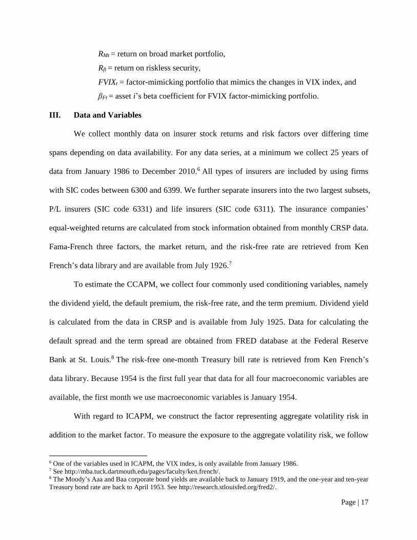
RMt = return on broad market portfolio,

Rft = return on riskless security,

FVIXt = factor-mimicking portfolio that mimics the changes in VIX index, and

βFt = asset i’s beta coefficient for FVIX factor-mimicking portfolio.

III. Data and Variables

We collect monthly data on insurer stock returns and risk factors over differing time

spans depending on data availability. For any data series, at a minimum we collect 25 years of

data from January 1986 to December 2010.6 All types of insurers are included by using firms

with SIC codes between 6300 and 6399. We further separate insurers into the two largest subsets,

P/L insurers (SIC code 6331) and life insurers (SIC code 6311). The insurance companies’

equal-weighted returns are calculated from stock information obtained from monthly CRSP data.

Fama-French three factors, the market return, and the risk-free rate are retrieved from Ken

French’s data library and are available from July 1926.7

To estimate the CCAPM, we collect four commonly used conditioning variables, namely

the dividend yield, the default premium, the risk-free rate, and the term premium. Dividend yield

is calculated from the data in CRSP and is available from July 1925. Data for calculating the

default spread and the term spread are obtained from FRED database at the Federal Reserve

Bank at St. Louis.8 The risk-free one-month Treasury bill rate is retrieved from Ken French’s

data library. Because 1954 is the first full year that data for all four macroeconomic variables are

available, the first month we use macroeconomic variables is January 1954.

With regard to ICAPM, we construct the factor representing aggregate volatility risk in

addition to the market factor. To measure the exposure to the aggregate volatility risk, we follow

6 One of the variables used in ICAPM, the VIX index, is only available from January 1986. 7 See http://mba.tuck.dartmouth.edu/pages/faculty/ken.french/. 8 The Moody’s Aaa and Baa corporate bond yields are available back to January 1919, and the one-year and ten-year

Treasury bond rate are back to April 1953. See http://research.stlouisfed.org/fred2/.

Page | 18

the literature (see, e.g., Breeden et al., 1989; Ang et al., 2006; Barinov, 2014) and create a factor-

mimicking portfolio, FVIX, using a set of base assets such that it is the portfolio of assets whose

returns are maximally correlated with realized innovations in market volatility. The base assets

are a small set of diversified portfolios that are sufficiently different from one another to reflect

information about different pieces of the economy. Their returns are not noisy because of their

diversified nature. The step-by-step formation of FVIX is as follows. First of all, we use the VIX

index as the proxy of aggregate/market volatility, which measures the implied volatility of the at-

the-money options on the S&P100 stock index. To measure the innovations to expected

aggregate volatility, we use daily changes in the VIX index available from the Chicago Board of

Options Exchange (CBOE). For a detailed description of VIX, see Whaley (2000) and Ang et al.

(2006). Secondly, following the literature we use the six Fama-French (1993) size and book-to-

market portfolios as our base assets, which are sorted in two groups on size and three groups on

book-to-market. The daily returns to these portfolios come from Ken French’s data library. Then

we form the factor-mimicking portfolio that tracks the daily changes in the VIX index. We

regress the VIX daily changes on the daily excess returns to our base assets. The fitted part of the

regression is the combination of the base assets with the most positive correlation with the VIX

change. Our aggregate volatility risk factor, FVIX, is the fitted part less the constant. Finally,

since the change in VIX is collected at the daily frequency to accurately proxy for the

innovations about VIX, the FVIX computed is on the daily basis as well. However, given that

daily returns are very noisy and that other variables in the models are monthly, we cumulate the

daily FVIX by adding them up to the monthly level to attain the FVIX factor.

Page | 19

IV. Model Performance Comparisons

In this part, we empirically show that the insurance industry as a whole is indeed

sensitive to time-varying economic, market, and aggregate volatility risk. Then we investigate

two major insurance industry sectors separately, namely publicly traded P/L insurers and life

insurers, to determine whether their risk sensitivities differ. Moreover, we compare the

performance of four different models (CAPM, FF3, CCAPM, and ICAPM) in term of alpha

(model intercept), explanatory power (model R-squared), and statistical significance (model t-

statistics). We demonstrate that multi-period models are more appropriate for insurance firms.

The data we used are from January 1986 to December 2010; hence we obtain up to 300

months of returns on each sample firms.9 The insurer monthly returns are winsorized at 1st and

99th percentiles. This procedure results in a range of monthly returns from -33.8 to 40 for all

individual insurers. For each month, three portfolio returns are generated based on equally

weighed individual insurer returns for all insurers, P/L insurers and life insurers, respectively.

The average number of firms in any month during this 25-year period is 166, 67, and 52 for all

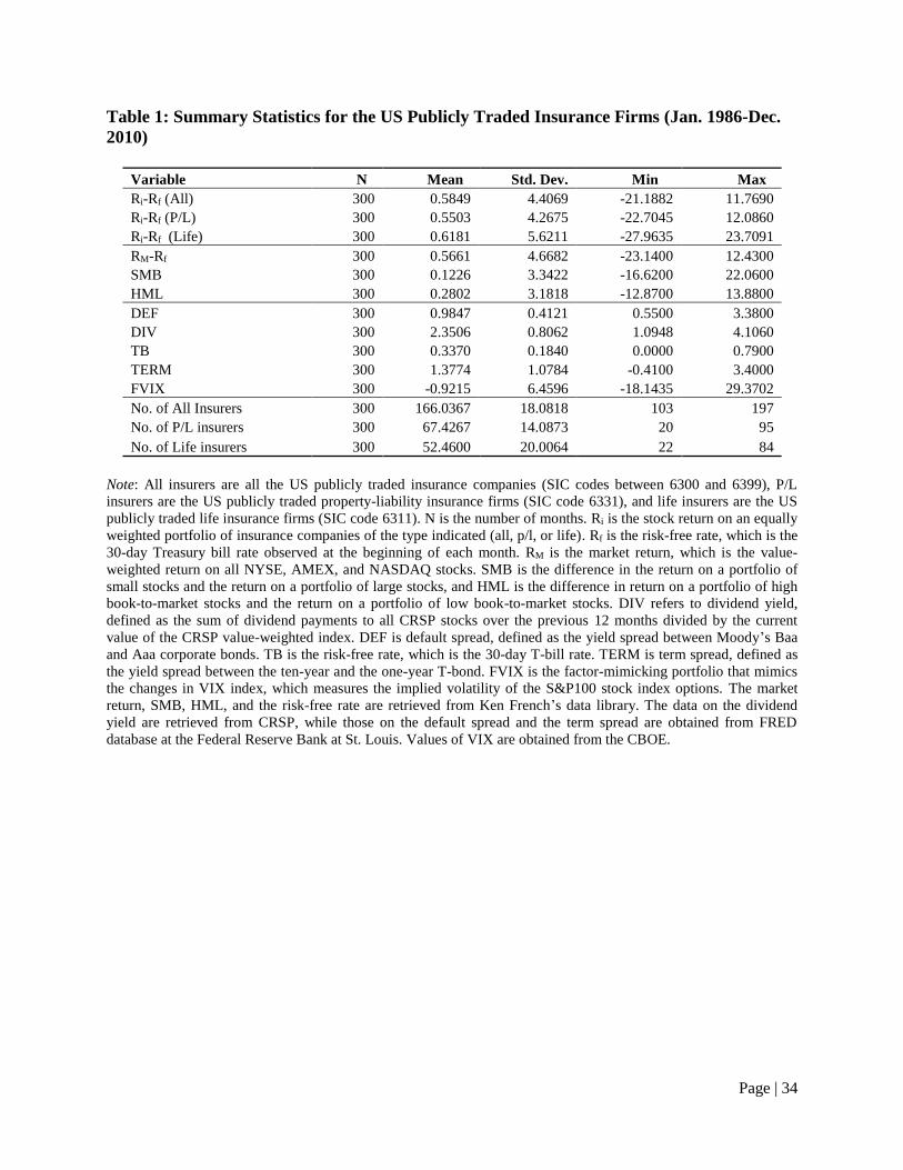
insurers, P/L insurers, and life insurers, respectively. Table 1 reports the summary statistics of

the returns to the insurance industry, market risk premium, Fama-French factors (i.e., SMB and

HML), macroeconomic variables, and FVIX. The summary statistics of the numbers of different

insurers are shown as well. From Table 1, we can see that the ranges of insurer excess returns,

market risk premium, and Fama-French factors are generally similar. The mean excess returns

for all insurers, P/L insurers, and life insurers are 0.58, 0.55, and 0.62 , respectively. The mean

monthly market risk premium is 0.57 during the sample period, almost identical to the mean for

all insurers.

9 We do not go back further in time because the VIX index is only available starting in January 1986. To compare

models over the same time period, we examine the 25-year period from January 1986 to December 2010 in the first

part of our empirical analysis (the model performance comparisons).

Page | 20

Tables 2, 3 and 4 report the regression results of four different asset pricing models for all

publicly traded insurers, P/L insurers, and life insurers, respectively. For all three insurer samples,

the coefficient on the market risk premium is positive, significant, and below one for the CAPM,

FF3, and ICAPM model, implying that the market or systematic risk of insurers, on average, is

less than the market as a whole based on these three models. The beta of CCAPM cannot be

directly observed in the regression results because it is a function of the macroeconomic

(conditioning) variables, as shown in Equation (6) above. According to Tables 2 through 4, in

FF3 the coefficients of all three factors are significantly positive at the 1 percent level.

As discussed earlier, CAPM and FF3 are single-period models. However, in reality

investment and consumption decisions are made over multiple periods, and the insurance

industry is exposed to business and economic cycles. Multi-period models, such as the CCAPM

and ICAPM, account for multiple periods and the time-varying risks. According to CCAPM, the

countercyclical beta, namely higher beta of insurers in recessions, is another source of risk in

addition to what is predicted by CAPM. Does the insurance industry have countercyclical beta?

First of all, the slopes on the products of the macroeconomic variables with the market excess

return demonstrate how the beta changes with different macroeconomic variables. Based on

Table 2 for all insurers, the CCAPM regression results indicate that the stock returns of insurance

companies significantly increase with the dividend yield and significantly decrease with the

Treasury bill rate; and are not significantly related to either the default premium or term

premium. These results show that insurers are exposed to dividend yield risk and interest rate

risk. Next, we examine whether insurers have countercyclical beta. Table 5 shows how to

determine the cyclicality of beta for companies based on modern asset pricing theories (see, e.g.,

Constantinides and Duffie, 1996; Campbell and Cochrane, 1999).

Page | 21

According to the stock market predictability literature (see, e.g., Fama and French, 1988,

1989), default spread, dividend yield, and term spread are high in economic recessions and low

in expansions. In contrast, Treasury bill rate is low in recessions and high in expansions. In

Section II, Equation (8) is obtained by rearranging Equation (7), which uses the expression of

beta from Equation (6). This indicates that coefficient signs of the macroeconomic variables

should be consistent across Equation (6), (7), and (8).10 If stock returns to the insurance industry

in Equation (8) are, and hence its market beta in Equation (6) is, positively correlated with the

default spread, dividend yield, or term spread, or negatively correlated with the Treasury bill rate,

it indicates that insurers’ market beta is high in recessions and low in expansions. Thus, as a

result, the insurers have countercyclical beta, and bear extra risk—the risk exposure increases in

bad times—based on CCAPM compared to what the CAPM predicts. In essence, the CCAPM

beta is allowed to vary with economic cycles. On the contrary, if the stock returns to the

insurance industry are negatively correlated with the default spread, dividend yield, or term

spread, or positively correlated with the Treasury bill rate, the insurers have procyclical beta, and

bear less risk based on CCAPM compared to what the CAPM predicts.

From Table 2, we see that the risk of insurance industry increases in recessions because

the coefficients of the product of dividend yield and market risk premium and the product of

Treasury bill rate and market risk premium are significantly positive and negative, respectively.

Moreover, the coefficient on market risk premium is positive, and correlation coefficient of the

insurer stock excess returns and market excess returns is positive. Therefore, dividend yield and

Treasury bill rate load positively and negatively on insurer stock returns, and hence insurer

market beta, demonstrating that the insurance industry has countercyclical beta and its risk

10 For example, the coefficient of the term with DEFt-1 in Equation (8), and the coefficients of DEFt-1 in Equation (7)

and (6) are all bi1. The same situation applies to the other three macroeconomic variables.

Page | 22

increases in recessions. That is to say, insurers are exposed to time-varying risks, which single-

period models, such as CAPM and FF3, do not incorporate. In this sense, CCAPM is superior to

single-period models when it comes to estimating the expected stock returns and cost of equity

for insurers.

From Table 2 we can also analyze the results of ICAPM. The negative FVIX beta of

insurance companies suggests that when volatility (VIX) increases unexpectedly, insurance firms

tend to have worse returns than firms with comparable CAPM betas, which makes insurance

companies riskier than what CAPM estimates. Even though FVIX is insignificant, the market

beta in ICAPM is smaller than the ones in CAPM, which means that FVIX shares the

explanatory power of market risk premium, and it does have impacts on insurer stock returns. In

sum, insurers are exposed to the time-varying risk, in particular, market aggregate volatility risk.

From a theoretical perspective, we claim that CCAPM and ICAPM are more appropriate

than single-period models given that they account for time-varying risks of insurers as

manifested in the significant factor loadings and the above analyses. From an empirical

perspective, are they also superior? As reported in Tables 2 to 4, alpha is not significant in any of

the four models. According to Fama and French (1993), if an asset pricing model is well-

specified, then its alpha should be indistinguishable from zero. Therefore, in regards to alpha,

CAPM, FF3, CCAPM, and ICAPM are equivalent in explaining insurer stock returns. Moreover,

for the regressions that include all insurers, Table 2, the adjusted R-squareds are 0.61, 0.78, 0.66,

and 0.61 for CAPM, FF3, CCAPM, and ICAPM, respectively. Even though FF3 has the highest

adjusted R-squared, all four models have relatively high explanatory power. 11 The pattern of the

11 Lewellen, Nagel, and Shanken (2010) point out that researchers should not rely too heavily on R-squared in asset

pricing tests, and suggest to evaluate in combination with other important tests, particularly with theoretical

guidance. Therefore, the highest adjusted R-squared of FF3 should not be regarded as the evidence that it is superior

to the others.

Page | 23

adjusted R-squared is similar in Tables 3 and 4 for P/L and life insurers; that is, the FF3 model

yields the highest and CCAPM the second highest with the CAPM and ICAPM having very

similar ones.

The CCAPM results for P/L insurers in Table 3 report that the coefficient for the product

of dividend yield and market excess returns is significantly positive. As true for the sample of all

types of insurers, these results suggest the countercyclicality of P/L insurers and that their risk

increases in recessions. For P/L insurers, ICAPM regression estimates indicate that FVIX loads

significantly negatively at the 5 percent level. This implies that when the stock market volatility

index (VIX) increases unexpectedly and when investors have to cut current consumptions and

save for the future, the portfolio of P/L insurance firms erodes further on the limited

consumption and spares even less for precautionary savings. They tend to have worse returns

than firms with comparable CAPM beta, which makes them riskier than what CAPM predicts.

Therefore, P/L insurer stock returns are sensitive to aggregate volatility risk. These additional

risks reflected in the CCAPM and ICAPM are ones that the single-period models do not

explicitly include.

Table 4 reports the regression results for the four asset pricing models for life insurers.

Again, the loading for market risk premium is significantly positive for CAPM, and those for

Fama-French three factors are significantly positive for FF3. It is worth noting that the market

betas for CAPM, FF3, and ICAPM are higher for life insurers than for P/L insurers, or all

insurers, indicating the life insurers face more market risk than other types of insurers based on

these all models. With regard to CCAPM, we observe that the coefficients for the products of the

market excess returns and the default spread, dividend yield, Treasury bill rate, and term spread

are significantly positive, positive, negative, and negative, respectively. According to Table 5

Page | 24

and earlier discussion of CCAPM, the coefficient signs on the default spread, dividend yield, and

Treasury bill rate imply that the risk of life insurers increases in recessions, while the coefficient

sign on the term spread suggests that the risk of life insurers decreases in recessions. Since the

magnitude and significance of the coefficients on the first three macroeconomic variables are

much larger than that on the term spread, we conclude that the life insurers, like P/L insurers,

have countercyclical beta, and that their risk increases in recessions. When looking at the

regression results of the ICAPM, we find that FVIX loads insignificantly negatively on the life

insurer stock returns. Even though FVIX is insignificant, the market beta in ICAPM is smaller

than the ones in CAPM and FF3, which means that FVIX shares part of the explanatory power of

the market risk premium, and it indeed impacts life insurer stock returns indirectly. In sum, life

insurers are exposed to the time-varying risk, an additional risk source recognized in the

CCAPM and ICAPM that the single-period models do not explicitly include.

V. Cost of Equity Estimation

Estimation Data and Methodologies

In the study, we estimate the insurer cost of equity for 11 years from 2000 to 2010. Our

general methodology closely follows Cummins and Phillips (2005). Slope coefficients, or betas,

for each of the four asset pricing models (CAPM, FF3, CCAPM and ICAPM) are estimated in

Ordinary Least Squares regressions over the past 60 months for each sample insurer. We use

insurance company monthly stock returns from July 1995 to June 2010 from the CRSP database

in the beta estimation regressions; the 60 month periods end in June of 2000, 2001, 2002, 2003,

2004, 2005, 2006, 2007, 2008, 2009 and, 2010, resulting in 11 different estimation periods. Like

Cummins and Phillips (2005), we require a minimum of 36 consecutive months of stock returns

for each sample firm. Estimated beta coefficients are winsorized at an absolute value of 5 (see,

Page | 25

e.g., Cummins and Phillips, 2005). We perform estimates for all types of publicly traded insurers

combined, and separately for P/L insurers and life insurers.

Once slope estimates are obtained based on regressions over 60 month periods, consistent

with existing literature, the cost of equity is estimated by multiplying the slope estimates with the

long-run average of the factor risk premiums.12 For all models, the market risk premium (market

return less risk-free rate) is averaged from July 1926 to the final month of each estimation period

(such as June 2008 for 2008 COE estimation), and the risk-free rate is the 60-month average

ending the final month of each estimation period. For FF3, averages on SMB and HML are

calculated from July 1926 to the end of each estimation period. For the CCAPM, the four

macroeconomic return variables are averaged over the 60 months ending in June of each

estimation period for purposes of calculating the CCAPM market beta as shown in Equation

(6).13 For the ICAPM, the FVIX factor is calculated from January 1986 to the final month of

each estimation period.14

Cost of Equity Estimation Results

We compare the COE estimates for the eleven years of estimation results individually

and in the aggregate. The CAPM is used as a benchmark model because it is the earliest of the

“modern” asset pricing in the field of financial economics, it is a single-period and one-factor

model, it is the most widely investigated cost of equity model in the academic literature, it is

12 Longer time periods are used to estimate risk premiums than regression coefficients, consistent with prior finance

and insurance literature on the cost of equity. The reason for this approach is that factor risk-premiums are expected

to be more stable than individual firm factor risk sensitivities. 13 Note that Equation (8) is first estimated in the firm-level regressions using monthly values of macroeconomic

variables during the past 60 months. The estimated parameters are then inserted back into Equation (6) to calculate

the CCAPM market beta. Finally, the CCAPM cost of equity is obtained by multiplying the estimated market beta

with the long-run market risk premium as in Equation (4). 14 To control for potential biases resulted from infrequent trading and for robustness check, following Cummins and

Phillips (2005), the betas of all four asset pricing models (CAPM, FF3, CCAPM, and ICAPM) are also estimated

using the widely accepted sum-beta approach. The estimated sum-beta coefficients are obtained by adding the

contemporaneous and lagged beta estimates from Equation (1), (2), (7), (8), and (9). The results of COE estimates

after the sum-beta approach adjustment do not qualitatively change.

Page | 26

widely used in practice, and it is commonly used as the benchmark model to which other models

are compared. We do, however, make some general comparisons of all four models.

The mean COE estimates for our sample of all publicly-traded insurers are presented in

Table 6 for each of the 11 years (2000-2010) and 11 years combined. We also report t-test and

Wilcoxon signed-rank test statistics comparing the FF3 model, CCAPM, and ICAPM to the

CAPM. We present cost of equity estimates winsorized at the 5th and 95th percentiles. The FF3

model produces highest mean COE estimates for each of the eleven years and for all eleven years

combined. It gives a mean COE for all eleven years of 13.72 percent, almost 450 basis points

higher than the ICAPM which yields the second highest 11-year average of 9.24. The FF3 model

mean (median) COE estimates are significantly higher than the CAPM for each year and for all

years combined at the 0.01 level. The CCAPM generated a mean COE estimate of 8.82, or

around 23 basis points higher than the CAPM, a difference significant at the 0.01 level. The

median COE estimates from CCAPM are significantly higher than those from CAPM by 31 basis

points. Looking at individual years, the CCAPM COE estimates are significantly higher (lower)

than the CAPM COE estimates in four (two) of the eleven years. The ICAPM produces a mean

(median) COE of 9.24 (8.90) percent for the entire 11-year period, and significantly higher COE

estimates than the CAPM in six (nine) of the eleven years based on comparisons of means

(medians). According to untabulated results, the difference between the maximum and minimum

mean COE estimates by model across the years ranges from about 350 basis points for the

CCAPM to 690 for the FF3 model. The mean differences among the CAPM, CCAPM and

ICAPM for all eleven years are below 100 basis points, but exceed 200 basis points in some

years. Therefore, for the all insurer sample, while the differences are statistically significant

Page | 27

between any two of the models, the substantially higher estimates from the FF3 are striking from

an economic perspective as well.

As mentioned in the Introduction, FF3 lacks ample theoretical foundation and the COE

estimates are short of unambiguous risk-based explanations. Moreover, FF3 is a single-period

model that does not explicitly recognize time-varying risks. Hence, we advocate that COE

estimates from multi-period models are more appropriate. However, company stakeholders can

still use FF3 estimates as a reference to make an informed decision. In Section IV we find that

insurance industry as a whole, as well as major sub-industries of P/L and life insurers, has

countercyclical beta. This is an additional risk to market risk embedded in CAPM, which

indicates that the risk exposure of insurers increases in bad times when bearing risk is especially

painful for investors. As a compensation for the undesirable behavior of such stocks, investors

demand an extra risk premium. This explains why our COE estimates from CCAPM are

significantly higher than those from CAPM in general. It is consistent with the theoretical

prediction in Equation (3). In Table 2 we find that FVIX factor does not load significantly on

stock returns of all publicly-traded insurer sample. However, FVIX does share explanatory

power from market risk factor. Therefore, we still suggest using ICAPM estimates as a reference

when making COE-related decisions for insurers.

The cost of equity estimates for the subsamples of P/L and life insurers are presented in

Tables 7 and 8, respectively. As with the all insurer sample, the FF3 model produces estimates

significantly higher than the other three models for each of the eleven years. An interesting

contrast, however, is that COE estimates for P/L insurers tend to be lower on average than for

life insurers. The mean COE estimates of the whole 11-year period for P/L insurers versus life

insurers are as follows: 8.01 v. 9.54 percent for the CAPM; 12.56 v. 15.03 percent for the FF3

Page | 28

model; 8.27 v. 9.32 percent for the CCAPM; and 8.70 v. 10.13 percent for the ICAPM. These

COE estimates suggest that the required rate of return for life insurers is higher than that of P/L

insurers, which in turn, suggests that life insurer stocks are riskier. These estimated COE

differences between P/L and life insurers are all significantly different at the 0.01 level using

unpaired t-test assuming heteroskedasticity.

For P/L insurers, mean and median COE estimates from the CCAPM and ICAPM are

significantly higher than the CAPM for all years combined. The mean COE spreads of CCAPM

and ICAPM compared with CAPM are 26 and 69 basis points, while the median spreads are 18

and 71 basis points. Among these years, CCAPM produces significantly higher (lower) mean

COE estimates in 4 years (1 year) than CAPM. It also generates significantly higher median

COE estimates in 5 years and no significantly lower estimates in any year than CAPM. Similar

to the explanations to the all insurer sample, these results reflect the risk premium for

countercyclical beta of P/L insurers recognized in CCAPM. With regards to ICAPM, it produces

significantly higher (lower) mean COE estimates in 6 years (2 year), and significantly higher

(lower) median COE estimates in 7 years (2 year) than CAPM. As shown in Table 3, P/L insurer

stock returns are significantly associated with FVIX factor, which means that P/L insurers are

sensitive to aggregate volatility risk. The significant higher COE estimates by ICAPM compared

to CAPM are due to the risk premium of exposure to aggregate volatility risk of P/L insurers. It

is the compensation for the risk that when bad news (surprise increase in aggregate volatility)

arrives the value of P/L insurance portfolio drops. Since, based on empirical results in Table 3,

both CCAPM and ICCAPM work well for P/L insurers, we suggest P/L insurer stakeholders

using COE estimates from both models when making related decisions.

Page | 29

For life insurers, mean and median COE estimates from the ICAPM are significantly

higher than the CAPM for all years combined. The mean and median spreads are 59 and 21 basis

points, respectively. Similar to all insurers and P/L insurers, ICAPM yields significantly greater

COE estimates than CAPM in most of the individual years. With regards to CCAPM, for some

of the single years it produces higher COE estimates than CAPM, while for some other years

lower. Further, there is not a significant difference between COE estimates based on the CCAPM

and CAPM for all years combined.

In general, our results with respect to multi-period models are consistent with the notion

that investors are rewarded extra risk premium for bearing time-varying risks that are not

explicitly recognized in single-period models. Note that in some individual years, multi-period

models do not yield strictly greater COE estimates than the CAPM. We summarize several

reasons as follows. First of all, models are not perfect, and any model is an approximation to

reality. The interesting question is how accurate a model is (see, Jagannathan and Wang, 1996).

Throughout this paper, we argue that multi-period models are closer to the reality, and more

exact and more appropriate in estimating COE. Second, model parameters, including slope

coefficients (i.e., betas) and factor risk premiums are estimates, and as such, subject to

measurement error. For example, neither the true beta nor the true expected market risk premium

is observable. Third, while our approach is consistent with the existing literature, historical betas

and risk premiums vary over different time periods, and such variations may reflect short-term

market behavior rather than long-run investor expectations. Further, the sample composition for

the 25 years of performance comparison regression is different from that for the 11 years of COE

estimates. It may result in some discrepancies. Lastly, the beta estimation in the performance

comparison regression is based on the past 25 years, while that in the COE estimates for each

Page | 30

year is based on the past 5 years. Especially for CCAPM, whether the past 5 years capture

variations in economic conditions is a question. However, in order to make comparable and

consistent comparison with CAPM and FF3 whose COE estimation method is well established in

the literature (see, e.g., Fama and French, 1997; Cummins and Phillips, 2005), we use the past 5

years.

VI. Summary and Conclusions

The importance of cost of equity to insurance company owners, managers and regulators

is widely recognized by academics and practitioners. We extend prior academic literature by

exploring multi-period asset pricing models and comparing them to single-period models. We

find that insurer stock returns are sensitive to time-varying macroeconomic and aggregate

volatility risks. More precisely, insurers’ risk exposure is higher in recessions as characterized by

higher default spreads, higher dividend yields, and higher term spreads, and low Treasury bill

rates, when bearing risk is especially costly. In other words, insurance company market betas are

countercyclical. Moreover, P/L insurance portfolio values decrease when current consumption

has to be cut in response to surprise increase in expected aggregate volatility. Therefore, P/L

insurers are riskier than what the CAPM predicts because their risk exposure rises when bad

news arrives. The two multi-period models examined (CCAPM and ICAPM) account for

additional time-varying systematic risks not accounted for in single-period models, such the

CAPM and FF3.

Our empirical evidence supports the value of using multi-period models to explain

insurer stock returns and to estimate insurer COE. Specifically, using 25 years of data we find

that the macroeconomic factors mentioned above have significant impacts on the ex post stock

returns of insurers, and insurers have countercyclical beta. Further, insurers are sensitive to the

Page | 31

aggregate volatility risk. While our empirical results indicate that the CCAPM and FF3 model

are comparable based on statistical criteria (alpha, explanatory power, and statistical

significance), economic theory gives more credence to the CCAPM because it explicitly

recognizes time-varying risks, which may be proxied for by the FF3 factors. Further, the

CCAPM risk factors have a natural economic interpretation. In addition, our findings suggest

that life insurer stock returns are more sensitive to macroeconomic risk factors than P/L insurer

stock returns. Both the FF3 model and the CCAPM explain more of the variation in life insurer

stock returns than in P/L insurer stock returns.

In relation to cost of equity estimates, based on an 11 year window, the FF3 model

generates the highest values, averaging around 400 basis points higher than the next highest

model. 11 year-average COE estimates from the other three models (CAPM, CCAPM and

ICAPM) are within 100 basis points of one another. Consistent with the notion that additional

time-varying risks require greater rewards, the average COE estimates from the CCAPM and

ICAPM are significantly higher than the ones from the CAPM. Each of the four asset pricing

models yield higher average COE estimates for life insurers than P/L insurers, suggesting that

life insurers are riskier, and consequently that investors require higher returns from life insurers.

Our results indicate that the two prevalent models (CAPM and FF3) used in the extant literature

produce widely different COE estimates. Specifically, on average, COE estimates based on

CAPM are the lowest and those based on FF3 are highest, with those based on the CCAPM or

ICAPM in the middle. As a result, in addition to the stronger theoretical appeal of the multi-

period models, they may also enable decision makers to more confidently estimate COE in a

narrower range, and at a level closer to the traditional CAPM rather than the FF3 model.

Page | 32

Our study adds to the existing literature in three ways. First, it is the first to examine

multi-period asset pricing models for insurance firms. Second, it provides empirical evidence in

support of the pricing of time-varying macroeconomic and aggregate volatility risks for insurers.

Third, it provides evidence of meaningful economic and statistical differences between single-

period and multi-period models. And, lastly, it demonstrates the practical importance of

generating COE estimates from a variety of models. These differences in COE estimates, at the

margin, determine whether investing and financing decisions insurers make increase or decrease

firm value.

References

Ali, A., L. Hwang, and, M. A. Trombley, 2003, Arbitrage Risk and the Book-to-Market Anomaly,

Journal of Financial Economics, 69: 355-373.

Ang, A., R. Hodrick, Y. Xing, and X. Zhang, 2006, The Cross-Section of Volatility and Expected Returns,

Journal of Finance, 61: 259-299.

Barinov, A., 2013, Analyst Disagreement and Aggregate Volatility Risk, Journal of Financial and

Quantitative Analysis, 48(6): 1877-1900.

Barinov, A., 2014, Turnover: Liquidity or Uncertainty? Management Science, forthcoming.

Berk, J. B., 1995, A Critique of Size-Related Anomalies, Review of Financial Studies, 8: 275-

286.

Breeden, D.T., 1979, An Intertemporal Asset Pricing Model with Stochastic Consumption and Investment

Opportunities, Journal of Financial Economics, 7, 265 – 296.

Breeden, D.T., M.R. Gibbons, and R.H. Litzenberger, 1989, Empirical Tests of the Consumption-

Oriented CAPM, Journal of Finance, 44: 231-262.

Brennan, M. J., A. W. Wang, and Y. Xia, 2004, Estimation and Test of a Simple Model of Intertemporal

Capital Asset Pricing, Journal of Finance, 59: 1743-1775.

Campbell, J. Y., 1987, Stock Returns and the Term Structure, Journal of Financial Economics, 18: 373–

399.

Campbell, J. Y., 1993, Intertemporal Asset Pricing without Consumption Data, American Economic

Review, 83: 487-512.

Campbell, J. Y., 1996, Understanding Risk and Return, Journal of Political Economy, 104: 298-345.

Campbell, J. Y., and J. H. Cochrane, 1999, By Force of Habit: A Consumption-based Explanation of

Aggregate Stock Market Behavior, Journal of Political Economy, 107 (2): 205–251.

Campbell, J. Y., A. W. Lo, and A. C. MacKinlay, 1997, The Econometrics of Financial Markets,

Princeton University Press.

Campbell, J. Y., C. Polk, and T. Vuolteenaho, 2010, Growth or Glamour? Fundamentals and

Systematic Risk in Stock Returns, Review of Financial Studies, 23: 305-344.

Chen, J., 2002, Intertemporal CAPM and the Cross-Section of Stock Returns, Working Paper, University

of Southern California.

Chen, N., R. Roll, and S. A. Ross, 1986, Economic Forces and the Stock Market, Journal of Business, 59:

383 – 403.

Page | 33

Cochrane, J. H., 2005, Asset Pricing, Princeton University Press, Princeton, NJ.

Cochrane, J. H., 2007, Financial Markets and the Real Economy, International Library of Critical

Writings in Financial Economics, London: Edward Elgar.

Constantinides, G. M., and D. Duffie, 1996, Asset Pricing with Heterogeneous Consumers, Journal of

Political Economy, 104 (2): 219–240.

Cummins, J. D., and R. D. Phillips, 2005, Estimating the Cost of Equity Capital for Property-Liability

Insurers, Journal of Risk and Insurance, 72 (3): 441-478.

Davis, J. L., E. F. Fama, and K. R. French, 2000, Characteristics, Covariances, and Average Returns:

1929-1997, Journal of Finance, 55: 389-406.

Eckbo, B. E., R. W. Masulis, and O. Norli, 2000, Seasoned Public Offerings: Resolution of the New

Issues Puzzle, Journal of Financial Economics, 56: 251-291.

Fama, E. F., 1981, Stock Returns, Real Activity, Inflation, and Money, American Economic Review, 71:

545–565.

Fama, E. F., and K. R. French, 1988, Dividend Yields and Expected Stock Returns, Journal of Financial

Economics, 22: 3–25.

Fama, E. F., and K. R. French, 1989, Business Conditions and Expected Returns on Stocks and

Bonds, Journal of Financial Economics, 25: 23-49.

Fama, E. F., and K. R. French, 1992, The Cross-Section of Expected Stock Returns, Journal of

Finance, 47 (2): 427–465.

Fama, E. F., and K. R. French, 1993, Common Risk Factors in the Returns on Stocks and Bonds, Journal

of Financial Economics, 33 (1): 3–56.

Fama, E. F., and K. R. French, 1995, Size and Book-to-Market Factors in Earnings and Returns, Journal

of Finance, 50 (1): 131-155.

Fama, E. F., and K. R. French, 1997, Industry Costs of Equity, Journal of Financial Economics, 43: 153-

193.

Fama, E. F., and G. W. Schwert, 1977, Asset Returns and Inflation, Journal of Financial Economics, 5:

115-146.

Jagannathan, R., and Z. Wang, 1996, The Conditional CAPM and the Cross-Section of Expected Returns,

Journal of Finance: 51: 3-54.

Keim, D. B., and Stambaugh, R. F., 1986, Predicting Returns in the Stock and Bond Markets, Journal of

Financial Economics, 17: 357–390.

Lamont, O.A., 2001, Economic Tracking Portfolios, Journal of Econometrics, 105: 161-184.

Leland, H. E., 1999, Beyond Mean-Variance: Performance Measurement in a Nonsymmetrical World,

Financial Analysts Journal, 55: 27-36.

Lewellen, J. W., S. Nagel, and J. Shanken, 2010, A Skeptical Appraisal of Asset Pricing Tests, Journal of

Financial Economics, 96: 175-194.

Markowitz, H., 1959, Portfolio Selection, New York: John Wiley & Sons.

Merton, R. C., 1973, An Intertemporal Capital Asset Pricing Model, Econometrica, 41: 867-887.

Petkova, R., and L. Zhang, 2005, Is Value Riskier than Growth? Journal of Financial Economics, 78:

187-202.

Ross, S.A., 1976, The Arbitrage Theory of Capital Asset Pricing, Journal of Economic Theory, 13: 341-

360.

Rubinstein, M., 1976, The Valuation of Uncertain Income Streams and the Pricing of Options, Bell

Journal of Economics, 7: 407-425.

Wen, M., A. D. Martin, G. Lai, and T. J. O’Brien, 2008, Estimating the Cost of Equity for Property-

Liability Insurance Companies, Journal of Risk and Insurance, 75, 1: 101-124.

Whaley, R., 2000, The Investor Fear Gauge, Journal of Portfolio Management, 26: 12-17.

Zhang, L., 2005, The Value Premium, Journal of Finance, 60: 67-103.

Page | 34

Table 1: Summary Statistics for the US Publicly Traded Insurance Firms (Jan. 1986-Dec.

2010)

Variable N Mean Std. Dev. Min Max

Ri-Rf (All) 300 0.5849 4.4069 -21.1882 11.7690

Ri-Rf (P/L) 300 0.5503 4.2675 -22.7045 12.0860

Ri-Rf (Life) 300 0.6181 5.6211 -27.9635 23.7091

RM-Rf 300 0.5661 4.6682 -23.1400 12.4300

SMB 300 0.1226 3.3422 -16.6200 22.0600

HML 300 0.2802 3.1818 -12.8700 13.8800

DEF 300 0.9847 0.4121 0.5500 3.3800

DIV 300 2.3506 0.8062 1.0948 4.1060

TB 300 0.3370 0.1840 0.0000 0.7900

TERM 300 1.3774 1.0784 -0.4100 3.4000

FVIX 300 -0.9215 6.4596 -18.1435 29.3702

No. of All Insurers 300 166.0367 18.0818 103 197

No. of P/L insurers 300 67.4267 14.0873 20 95

No. of Life insurers 300 52.4600 20.0064 22 84

Note: All insurers are all the US publicly traded insurance companies (SIC codes between 6300 and 6399), P/L

insurers are the US publicly traded property-liability insurance firms (SIC code 6331), and life insurers are the US

publicly traded life insurance firms (SIC code 6311). N is the number of months. Ri is the stock return on an equally

weighted portfolio of insurance companies of the type indicated (all, p/l, or life). Rf is the risk-free rate, which is the

30-day Treasury bill rate observed at the beginning of each month. RM is the market return, which is the value-

weighted return on all NYSE, AMEX, and NASDAQ stocks. SMB is the difference in the return on a portfolio of

small stocks and the return on a portfolio of large stocks, and HML is the difference in return on a portfolio of high

book-to-market stocks and the return on a portfolio of low book-to-market stocks. DIV refers to dividend yield,

defined as the sum of dividend payments to all CRSP stocks over the previous 12 months divided by the current

value of the CRSP value-weighted index. DEF is default spread, defined as the yield spread between Moody’s Baa

and Aaa corporate bonds. TB is the risk-free rate, which is the 30-day T-bill rate. TERM is term spread, defined as

the yield spread between the ten-year and the one-year T-bond. FVIX is the factor-mimicking portfolio that mimics

the changes in VIX index, which measures the implied volatility of the S&P100 stock index options. The market

return, SMB, HML, and the risk-free rate are retrieved from Ken French’s data library. The data on the dividend

yield are retrieved from CRSP, while those on the default spread and the term spread are obtained from FRED

database at the Federal Reserve Bank at St. Louis. Values of VIX are obtained from the CBOE.

Page | 35

Table 2: Asset-Pricing Model Performance Comparison for All Publicly Traded Insurers

(Jan. 1986-Dec. 2010; N=300 months)

CAPM

Fama-French 3

Conditonal

CAPM

Intertemporal

CAPM

Alpha 0.1670

-0.0808

0.0751

0.1530

(0.1600)

(0.1208)

(0.1527)

(0.1607)

RM - Rf 0. 7382 *** 0.8082 *** 0.6600 *** 0.6286 ***

(0.0341)

(0.0269)

(0.1806)

(0.1214)

SMB

0.3083 ***

(0.0382)

HML

0.6080 ***

(0.0408)

DEFt-1*(RM - Rf)

-0.0104

(0.0764)

DIVt-1*(RM - Rf)

0.2565 ***

(0.0634)

TBt-1*(RM - Rf)

-1.2655 ***

(0.4015)

TERMt-1*(RM - Rf)

-0.0595

(0.0643)

FVIX

-0.0825

(0.0877)

Adjusted R-squared 0.6102 0.7821 0.6590 0.6101

Note: This table shows the regression results based on CAPM, FF3 model, CCAPM, and ICAPM with

FVIX for all the publicly traded insurance companies (SIC codes between 6300 and 6399), property-

liability insurers (SIC code 6331), and life insurers (SIC code 6311). The 30-day Treasury bill rate

observed at the beginning of each month is used as risk-free rate, and the market return is the value-

weighted return on all NYSE, AMEX, and NASDAQ stocks. In FF3, SMB is the difference in the

return on a portfolio of small stocks and the return on a portfolio of large stocks, and HML is the

difference in the return on a portfolio of high book-to-market stocks and the return on a portfolio of

low book-to-market stocks. We use four macroeconomic variables as conditioning variables in the

CCAPM, which include dividend yield (DIV), defined as the sum of dividend payments to all CRSP

stocks over the previous 12 months divided by the current value of the CRSP value-weighted index,

default spread (DEF), defined as the yield spread between Moody’s Baa and Aaa corporate bonds, risk-

free rate (TB), which is the 30-day T-bill rate, and term spread (TERM), defined as the yield spread

between the ten-year and the one-year T-bond. In the ICAPM, FVIX is the factor-mimicking portfolio

that mimics the changes in VIX index, which measures the implied volatility of the S&P100 stock

index options. The market return, SMB, HML, and the risk-free rate are retrieved from Ken French’s

data library. The data on the dividend yield are retrieved from CRSP, while those on the default spread

and the term spread are obtained from FRED database at the Federal Reserve Bank at St. Louis. Values

of VIX are obtained from the CBOE. Standard errors appear in brackets. ∗∗∗, ∗∗, and ∗ denote

statistical significance at the 1, 5, and 10 percent levels, respectively.

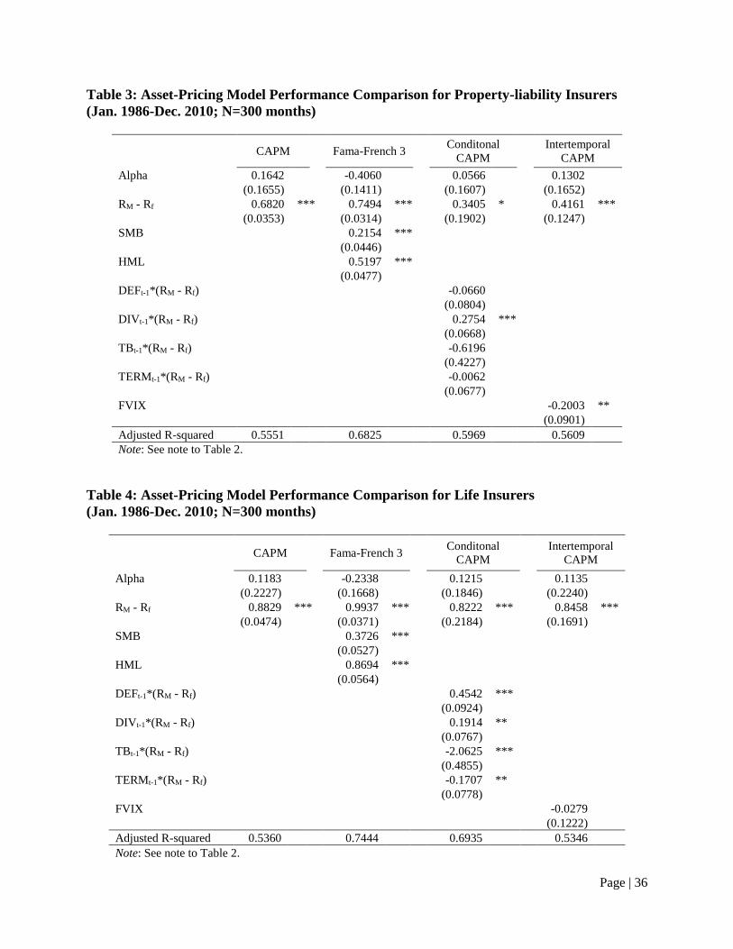
Page | 36

Table 3: Asset-Pricing Model Performance Comparison for Property-liability Insurers

(Jan. 1986-Dec. 2010; N=300 months)

CAPM

Fama-French 3

Conditonal

CAPM

Intertemporal

CAPM

Alpha 0.1642

-0.4060

0.0566

0.1302

(0.1655)

(0.1411)

(0.1607)

(0.1652)

RM - Rf 0.6820 *** 0.7494 *** 0.3405 * 0.4161 ***

(0.0353)

(0.0314)

(0.1902)

(0.1247)

SMB

0.2154 ***

(0.0446)

HML

0.5197 ***

(0.0477)

DEFt-1*(RM - Rf)

-0.0660

(0.0804)

DIVt-1*(RM - Rf)

0.2754 ***

(0.0668)

TBt-1*(RM - Rf)

-0.6196

(0.4227)

TERMt-1*(RM - Rf)

-0.0062

(0.0677)

FVIX

-0.2003 **

(0.0901)

Adjusted R-squared 0.5551 0.6825 0.5969 0.5609

Note: See note to Table 2.

Table 4: Asset-Pricing Model Performance Comparison for Life Insurers

(Jan. 1986-Dec. 2010; N=300 months)

CAPM

Fama-French 3

Conditonal

CAPM

Intertemporal

CAPM

Alpha 0.1183

-0.2338

0.1215

0.1135

(0.2227)

(0.1668)

(0.1846)

(0.2240)

RM - Rf 0.8829 *** 0.9937 *** 0.8222 *** 0.8458 ***

(0.0474)

(0.0371)

(0.2184)

(0.1691)

SMB

0.3726 ***

(0.0527)

HML

0.8694 ***

(0.0564)

DEFt-1*(RM - Rf)

0.4542 ***

(0.0924)

DIVt-1*(RM - Rf)

0.1914 **

(0.0767)

TBt-1*(RM - Rf)

-2.0625 ***

(0.4855)

TERMt-1*(RM - Rf)

-0.1707 **

(0.0778)

FVIX

-0.0279

(0.1222)

Adjusted R-squared 0.5360 0.7444 0.6935 0.5346

Note: See note to Table 2.

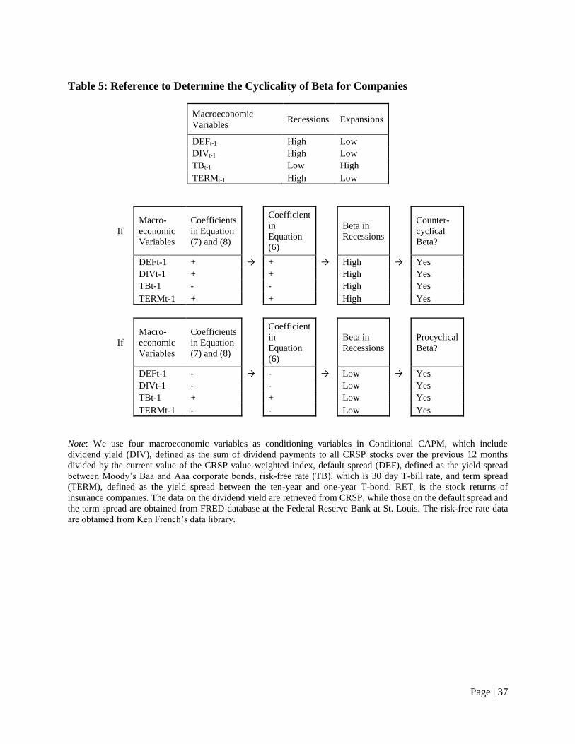
Page | 37

Table 5: Reference to Determine the Cyclicality of Beta for Companies

Macroeconomic

Variables Recessions Expansions

DEFt-1 High Low

DIVt-1 High Low

TBt-1 Low High

TERMt-1 High Low

If

Macro-

economic

Variables

Coefficients

in Equation

(7) and (8)

Coefficient

in

Equation

(6)

Beta in

Recessions

Counter-

cyclical

Beta?

DEFt-1 + → + → High → Yes

DIVt-1 +

+

High

Yes

TBt-1 -

-

High

Yes

TERMt-1 +

+

High

Yes

If

Macro-

economic

Variables

Coefficients

in Equation

(7) and (8)

Coefficient

in

Equation

(6)

Beta in

Recessions

Procyclical

Beta?

DEFt-1 - → - → Low → Yes

DIVt-1 -

-

Low

Yes

TBt-1 +

+

Low

Yes

TERMt-1 -

-

Low

Yes

Note: We use four macroeconomic variables as conditioning variables in Conditional CAPM, which include

dividend yield (DIV), defined as the sum of dividend payments to all CRSP stocks over the previous 12 months

divided by the current value of the CRSP value-weighted index, default spread (DEF), defined as the yield spread

between Moody’s Baa and Aaa corporate bonds, risk-free rate (TB), which is 30 day T-bill rate, and term spread

(TERM), defined as the yield spread between the ten-year and one-year T-bond. RETt is the stock returns of

insurance companies. The data on the dividend yield are retrieved from CRSP, while those on the default spread and

the term spread are obtained from FRED database at the Federal Reserve Bank at St. Louis. The risk-free rate data

are obtained from Ken French’s data library.

Page | 38

Table 6: Cost of Equity Estimates for All Publicly Traded Insurers

Year N CAPM

(1)

FF3

(2)

CCAPM

(3)

ICAPM

(4)

(1)-(2) (1)-(3) (1)-(4)

Mean Median Mean Median Mean Median

2010 152 9.6016 11.2136 9.1900 9.7152 -1.6120*** -1.0154*** 0.4116* 0.0616*** -0.1136 -0.1177*

2009 156 10.0675 11.8056 8.7979 10.1664 -1.7381*** -1.3067*** 1.2696*** 0.3735*** -0.0989 -0.0584**

2008 152 10.6081 12.7606 10.4825 10.8568 -2.1525*** -1.9707*** 0.1256 0.2635* -0.2487* -0.4578*

2007 153 9.5166 11.6599 10.3082 7.9706 -2.1434*** -1.5821*** -0.7917*** -0.6299*** 1.5460*** 1.2864***

2006 147 7.7246 11.1693 8.7966 5.7482 -3.4446*** -3.2229*** -1.0720*** -1.3369*** 1.9764*** 1.5089***

2005 146 6.4678 12.4130 8.1047 6.9940 -5.9453*** -5.7843*** -1.6370*** -1.6571*** -0.5263 -1.0122**

2004 142 6.4360 13.3094 7.5906 8.5794 -6.8734*** -6.7627*** -1.1546*** -0.9348*** -2.1434*** -1.8553***

2003 145 6.9984 14.5264 7.0077 8.7657 -7.5280*** -7.2989*** -0.0093 0.0039 -1.7673*** -1.6404***

2002 159 7.2863 16.1106 7.3231 9.3275 -8.8243*** -8.3962*** -0.0368 -0.3439 -2.0412*** -2.0824***

2001 153 9.0660 18.0298 8.7782 11.3184 -8.9638*** -8.8831*** 0.2878 0.3189 -2.2524*** -2.2718***

2000 162 10.2953 17.4643 10.4343 11.7547 -7.1690*** -7.0621*** -0.1390 0.1926 -1.4594*** -1.0562***

All Years 1667 8.5905 13.7190 8.8231 9.2423 -5.1284*** -5.1000*** -0.2325*** -0.3079*** -0.6518*** -0.7862***

Note: This table shows average cost of equity estimates for all publicly traded insurance companies based on CAPM, FF3 model, CCAPM, and ICAPM with

FVIX. Cost of equity is calculated for each firm according to Equations (1), (2), (7), (8), and (9). The 30-day Treasury bill rate observed at the beginning of each

month is used as risk-free rate, and the market return is the value-weighted return on all NYSE, AMEX, and NASDAQ stocks. N is the number of firms. In FF3,

SMB is the difference in the return on a portfolio of small stocks and the return on a portfolio of large stocks, and HML is the difference in the return on a

portfolio of high book-to-market stocks and the return on a portfolio of low book-to-market stocks. We use four macroeconomic variables as conditioning

variables in CCAPM, which include dividend yield (DIV), defined as the sum of dividend payments to all CRSP stocks over the previous 12 months divided by

the current value of the CRSP value-weighted index, default spread (DEF), defined as the yield spread between Moody’s Baa and Aaa corporate bonds, risk-free

rate (TB), which is 30-day T-bill rate, and term spread (TERM), defined as the yield spread between the ten-year and one-year T-bond. In the ICAPM, FVIX is

the factor-mimicking portfolio of stocks that mimics the changes in the VIX index, which measures the implied volatility of the S&P100 index options. Values of

VIX are obtained from the CBOE. The market return, SMB, HML, and the risk-free rate are retrieved from Ken French’s data library. The data on the dividend

yield are retrieved from CRSP, while those on the default spread and the term spread are obtained from FRED database at the Federal Reserve Bank at St. Louis.

The data period for each year ends on June 30. Estimates are calculated using the previous 60-months of returns. If some returns are missing for individual firms,

at least 36 consecutive months are required. The risk-free rate used to estimate the cost of equity is the average 30-day T-bill rate from the first to the last month

of each 60-month estimation period. The market risk premium, SMB, and HML are calculated from July 1926 to the final month of each estimation period. The

four macroeconomic variables are averaged over the 60 months ending in the last month of each estimation period. FVIX is calculated from January 1986 to the

final month of each estimation period.

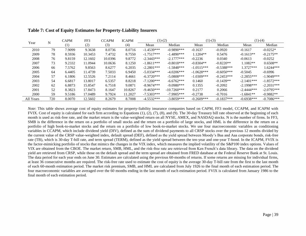
Page | 39

Table 7: Cost of Equity Estimates for Property-Liability Insurers

Year N CAPM

(1)

FF3

(2)

CCAPM

(3)

ICAPM

(4)

(1)-(2) (1)-(3) (1)-(4)

Mean Median Mean Median Mean Median

2010 79 7.9099 9.3638 8.0736 8.0716 -1.4539*** -0.9890*** -0.1637 -0.0920 -0.1617 -0.0252*

2009 78 8.5936 10.3453 7.4732 8.7550 -1.7517*** -1.4890*** 1.1204** 0.5476 -0.1613** -0.2175**

2008 76 9.8159 12.1602 10.0396 9.8772 -2.3443*** -2.1777*** -0.2236 0.0340 -0.0613 -0.0252

2007 73 9.2332 11.0944 10.0636 8.1250 -1.8611*** -0.8018*** -0.8304** -0.8220** 1.1082** 0.6508**

2006 66 7.5762 9.8563 8.6277 6.2035 -2.2801*** -1.5848*** -1.0515*** -0.5388*** 1.3727*** 1.6244***

2005 64 6.4405 11.4739 7.5033 6.9450 -5.0334*** -4.0206*** -1.0628*** -0.6050*** -0.5045 -0.6996

2004 57 6.1806 12.5526 7.2114 8.4661 -6.3720*** -5.0808*** -1.0309*** -0.2453*** -2.2855*** -1.9049***

2003 54 6.6817 13.8017 6.5357 8.8218 -7.1200*** -6.6762*** 0.1460 -0.1439** -2.1401*** -1.8572***

2002 62 6.8873 15.8547 6.7518 9.0871 -8.9674*** -9.0980*** 0.1355 -0.2092 -2.1998*** -2.2031***

2001 52 8.3823 17.8473 8.1647 10.8267 -9.4650*** -10.7260*** 0.2177 0.2066 -2.4444*** -2.0795***

2000 59 9.5186 17.0489 9.7924 11.2027 -7.5303*** -7.9905*** -0.2738 -0.7016 -1.6841** -0.9882**

All Years 720 8.0070 12.5602 8.2679 8.7008 -4.5532*** -3.8059*** -0.2609*** -0.1837*** -0.6938*** -0.7086***

Note: This table shows average cost of equity estimates for property-liability insurance companies based on CAPM, FF3 model, CCAPM, and ICAPM with

FVIX. Cost of equity is calculated for each firm according to Equations (1), (2), (7), (8), and (9). The 30-day Treasury bill rate observed at the beginning of each

month is used as risk-free rate, and the market return is the value-weighted return on all NYSE, AMEX, and NASDAQ stocks. N is the number of firms. In FF3,

SMB is the difference in the return on a portfolio of small stocks and the return on a portfolio of large stocks, and HML is the difference in the return on a

portfolio of high book-to-market stocks and the return on a portfolio of low book-to-market stocks. We use four macroeconomic variables as conditioning

variables in CCAPM, which include dividend yield (DIV), defined as the sum of dividend payments to all CRSP stocks over the previous 12 months divided by

the current value of the CRSP value-weighted index, default spread (DEF), defined as the yield spread between Moody’s Baa and Aaa corporate bonds, risk-free

rate (TB), which is 30-day T-bill rate, and term spread (TERM), defined as the yield spread between the ten-year and one-year T-bond. In the ICAPM, FVIX is

the factor-mimicking portfolio of stocks that mimics the changes in the VIX index, which measures the implied volatility of the S&P100 index options. Values of

VIX are obtained from the CBOE. The market return, SMB, HML, and the risk-free rate are retrieved from Ken French’s data library. The data on the dividend

yield are retrieved from CRSP, while those on the default spread and the term spread are obtained from FRED database at the Federal Reserve Bank at St. Louis.

The data period for each year ends on June 30. Estimates are calculated using the previous 60-months of returns. If some returns are missing for individual firms,

at least 36 consecutive months are required. The risk-free rate used to estimate the cost of equity is the average 30-day T-bill rate from the first to the last month

of each 60-month estimation period. The market risk premium, SMB, and HML are calculated from July 1926 to the final month of each estimation period. The

four macroeconomic variables are averaged over the 60 months ending in the last month of each estimation period. FVIX is calculated from January 1986 to the

final month of each estimation period.

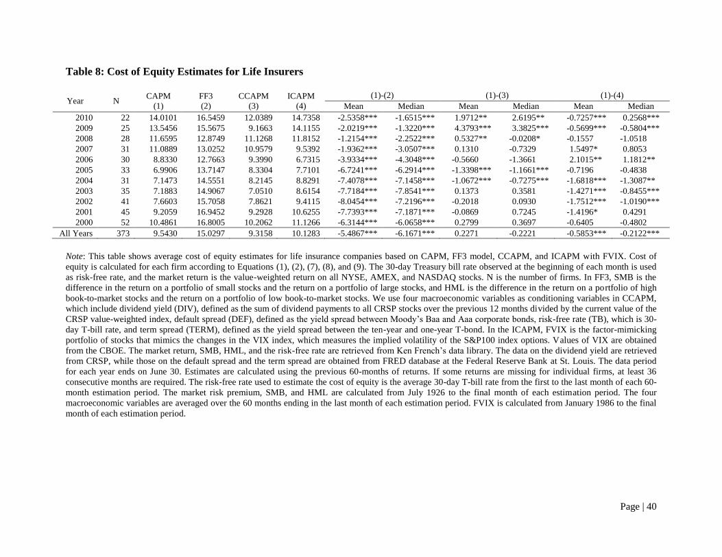
Page | 40

Table 8: Cost of Equity Estimates for Life Insurers

Year N CAPM

(1)

FF3

(2)

CCAPM

(3)

ICAPM

(4)

(1)-(2) (1)-(3) (1)-(4)

Mean Median Mean Median Mean Median

2010 22 14.0101 16.5459 12.0389 14.7358 -2.5358*** -1.6515*** 1.9712** 2.6195** -0.7257*** 0.2568***

2009 25 13.5456 15.5675 9.1663 14.1155 -2.0219*** -1.3220*** 4.3793*** 3.3825*** -0.5699*** -0.5804***

2008 28 11.6595 12.8749 11.1268 11.8152 -1.2154*** -2.2522*** 0.5327** -0.0208* -0.1557 -1.0518

2007 31 11.0889 13.0252 10.9579 9.5392 -1.9362*** -3.0507*** 0.1310 -0.7329 1.5497* 0.8053

2006 30 8.8330 12.7663 9.3990 6.7315 -3.9334*** -4.3048*** -0.5660 -1.3661 2.1015** 1.1812**

2005 33 6.9906 13.7147 8.3304 7.7101 -6.7241*** -6.2914*** -1.3398*** -1.1661*** -0.7196 -0.4838

2004 31 7.1473 14.5551 8.2145 8.8291 -7.4078*** -7.1458*** -1.0672*** -0.7275*** -1.6818*** -1.3087**

2003 35 7.1883 14.9067 7.0510 8.6154 -7.7184*** -7.8541*** 0.1373 0.3581 -1.4271*** -0.8455***

2002 41 7.6603 15.7058 7.8621 9.4115 -8.0454*** -7.2196*** -0.2018 0.0930 -1.7512*** -1.0190***

2001 45 9.2059 16.9452 9.2928 10.6255 -7.7393*** -7.1871*** -0.0869 0.7245 -1.4196* 0.4291

2000 52 10.4861 16.8005 10.2062 11.1266 -6.3144*** -6.0658*** 0.2799 0.3697 -0.6405 -0.4802

All Years 373 9.5430 15.0297 9.3158 10.1283 -5.4867*** -6.1671*** 0.2271 -0.2221 -0.5853*** -0.2122***

Note: This table shows average cost of equity estimates for life insurance companies based on CAPM, FF3 model, CCAPM, and ICAPM with FVIX. Cost of

equity is calculated for each firm according to Equations (1), (2), (7), (8), and (9). The 30-day Treasury bill rate observed at the beginning of each month is used

as risk-free rate, and the market return is the value-weighted return on all NYSE, AMEX, and NASDAQ stocks. N is the number of firms. In FF3, SMB is the

difference in the return on a portfolio of small stocks and the return on a portfolio of large stocks, and HML is the difference in the return on a portfolio of high

book-to-market stocks and the return on a portfolio of low book-to-market stocks. We use four macroeconomic variables as conditioning variables in CCAPM,

which include dividend yield (DIV), defined as the sum of dividend payments to all CRSP stocks over the previous 12 months divided by the current value of the

CRSP value-weighted index, default spread (DEF), defined as the yield spread between Moody’s Baa and Aaa corporate bonds, risk-free rate (TB), which is 30-

day T-bill rate, and term spread (TERM), defined as the yield spread between the ten-year and one-year T-bond. In the ICAPM, FVIX is the factor-mimicking

portfolio of stocks that mimics the changes in the VIX index, which measures the implied volatility of the S&P100 index options. Values of VIX are obtained

from the CBOE. The market return, SMB, HML, and the risk-free rate are retrieved from Ken French’s data library. The data on the dividend yield are retrieved

from CRSP, while those on the default spread and the term spread are obtained from FRED database at the Federal Reserve Bank at St. Louis. The data period

for each year ends on June 30. Estimates are calculated using the previous 60-months of returns. If some returns are missing for individual firms, at least 36

consecutive months are required. The risk-free rate used to estimate the cost of equity is the average 30-day T-bill rate from the first to the last month of each 60-

month estimation period. The market risk premium, SMB, and HML are calculated from July 1926 to the final month of each estimation period. The four

macroeconomic variables are averaged over the 60 months ending in the last month of each estimation period. FVIX is calculated from January 1986 to the final

month of each estimation period.