essays in applied financial econometrics
TRANSCRIPT

Essays in Applied Financial Econometrics
by
Lily Yanli Liu
Department of EconomicsDuke University
Date:Approved:
Andrew J. Patton, Supervisor
Tim Bollerslev
Jia Li
George Tauchen
Dissertation submitted in partial fulfillment of the requirements for the degree ofDoctor of Philosophy in the Department of Economics
in the Graduate School of Duke University2015

Abstract
Essays in Applied Financial Econometrics
by
Lily Yanli Liu
Department of EconomicsDuke University
Date:Approved:
Andrew J. Patton, Supervisor
Tim Bollerslev
Jia Li
George Tauchen
An abstract of a dissertation submitted in partial fulfillment of the requirements forthe degree of Doctor of Philosophy in the Department of Economics
in the Graduate School of Duke University2015

Copyright c© 2015 by Lily Yanli LiuAll rights reserved except the rights granted by the
Creative Commons Attribution-Noncommercial Licence

Abstract
This dissertation studies applied econometric problems in volatility estimation and
CDS pricing. The first chapter studies estimation of loss given default from CDS
spreads for U.S. corporates. This paper combines a term structure model of credit
default swaps (CDS) with weak-identification robust methods to jointly estimate the
probability of default and the loss given default of the underlying firm. The model
is not globally identified because it forgoes parametric time series restrictions that
have ensured identification in previous studies, but that are also difficult to verify in
the data. The empirical results show that informative (small) confidence sets for loss
given default are estimated for half of the firm-months in the sample, and most of
these do not include the conventional value of 0.60. In addition, risk-neutral default
probabilities, and hence risk premia on default probabilities, are underestimated
when loss given default is exogenously fixed at the conventional value instead of
estimated from the data.
The second chapter, which is joint work with Andrew Patton and Kevin Shep-
phard, studies the accuracy of a wide variety of estimators of asset price variation
constructed from high-frequency data (so-called “realized measures”), and compare
them with a simple “realized variance” (RV) estimator. In total, we consider over
400 different estimators, applied to 11 years of data on 31 different financial assets
spanning five asset classes, including equities, equity indices, exchange rates and in-
terest rates. We apply data-based ranking methods to the realized measures and to
iv

forecasts based on these measures. When 5-minute RV is taken as the benchmark
realized measure, we find little evidence that it is outperformed by any of the other
measures. When using inference methods that do not require specifying a bench-
mark, we find some evidence that more sophisticated realized measures significantly
outperform 5-minute RV. In forecasting applications, we find that a low frequency
“truncated” RV outperforms most other realized measures. Overall, we conclude
that it is difficult to significantly beat 5-minute RV for these assets.
v

To my mother, and in memory of my father.
vi

Contents
Abstract iv
List of Tables x
List of Figures xii
Acknowledgements xv
1 Estimating Loss Given Default from CDS under Weak Identifica-tion 1
1.1 Introduction . . . . . . . . . . . . . . . . . . . . . . . . . . . . . . . . 1
1.2 Credit Default Swaps and Spread Data . . . . . . . . . . . . . . . . . 6
1.2.1 CDS spread data description . . . . . . . . . . . . . . . . . . . 7
1.2.2 Summary Statistics for CDS spreads . . . . . . . . . . . . . . 9
1.3 CDS Term Structure Model . . . . . . . . . . . . . . . . . . . . . . . 10
1.3.1 A discrete-time framework for default . . . . . . . . . . . . . . 10
1.3.2 A factor model for the term structure of default probabilities . 13
1.3.3 Nelson-Siegel curves: a level-slope-curvature model . . . . . . 14
1.3.4 Joint Identification of Default Probabilities and Loss GivenDefault . . . . . . . . . . . . . . . . . . . . . . . . . . . . . . . 17
1.4 Robust Inference under Weak Identification . . . . . . . . . . . . . . 18
1.4.1 S-test robust to weak identification . . . . . . . . . . . . . . . 18
1.4.2 Estimation procedure for confidence sets for LGD . . . . . . . 22
1.4.3 Examples of Profile S-functions and S-sets . . . . . . . . . . . 24
vii

1.5 Empirical Results from Joint Estimation . . . . . . . . . . . . . . . . 24
1.5.1 Confidence Set Lengths and Locations . . . . . . . . . . . . . 25
1.5.2 Is loss given default really 0.60? . . . . . . . . . . . . . . . . . 26
1.5.3 Confidence sets across reference entities and over time . . . . . 27
1.5.4 Effects of CDS data characteristics on Confidence Set Size . . 29
1.5.5 Estimated default probability term structure . . . . . . . . . . 31
1.5.6 Discussion of risk premia implications . . . . . . . . . . . . . . 32
1.5.7 Firm characteristics and credit rating effects . . . . . . . . . . 35
1.6 Robustness Checks and Other Extensions . . . . . . . . . . . . . . . . 38
1.6.1 Alternate Nelson-Siegel Curves . . . . . . . . . . . . . . . . . 39
1.6.2 Varying the duration of the constant parameter assumption . 40
1.6.3 Model Extensions with additional degrees of freedom . . . . . 40
1.6.4 Further data and model extensions . . . . . . . . . . . . . . . 42
1.7 Conclusion . . . . . . . . . . . . . . . . . . . . . . . . . . . . . . . . . 44
1.8 Tables . . . . . . . . . . . . . . . . . . . . . . . . . . . . . . . . . . . 45
1.9 Figures . . . . . . . . . . . . . . . . . . . . . . . . . . . . . . . . . . . 51
2 Does Anything Beat 5-Minute RV? A Comparison of Realized Mea-sures Across Multiple Asset Classes 60
2.1 Introduction . . . . . . . . . . . . . . . . . . . . . . . . . . . . . . . . 60
2.2 Measures of asset price variability . . . . . . . . . . . . . . . . . . . . 64
2.2.1 Sampling frequency, sampling scheme, and sub-sampling . . . 64
2.2.2 Classes of realized measures . . . . . . . . . . . . . . . . . . . 66
2.2.3 Additional realized measures . . . . . . . . . . . . . . . . . . . 70
2.3 Comparing the accuracy of realized measures . . . . . . . . . . . . . . 72
2.3.1 Comparing estimation accuracy . . . . . . . . . . . . . . . . . 72
2.3.2 Comparing forecast accuracy . . . . . . . . . . . . . . . . . . . 74
viii

2.4 Data description . . . . . . . . . . . . . . . . . . . . . . . . . . . . . 74
2.5 Empirical results on the accuracy of realized measures . . . . . . . . . 77
2.5.1 Rankings of average accuracy . . . . . . . . . . . . . . . . . . 77
2.5.2 Pair-wise comparisons of realized measures . . . . . . . . . . . 78
2.5.3 Does anything beat 5-minute RV? . . . . . . . . . . . . . . . . 80
2.5.4 Estimating the set of best realized measures . . . . . . . . . . 84
2.5.5 Explaining performance differences . . . . . . . . . . . . . . . 86
2.5.6 Out-of-sample forecasting with realized measures . . . . . . . 92
2.6 Summary and conclusion . . . . . . . . . . . . . . . . . . . . . . . . . 96
2.7 Tables . . . . . . . . . . . . . . . . . . . . . . . . . . . . . . . . . . . 99
2.8 Figures . . . . . . . . . . . . . . . . . . . . . . . . . . . . . . . . . . . 114
A Appendix for Chapter 1 116
A.1 Additional Tables and Figures . . . . . . . . . . . . . . . . . . . . . . 117
B Appendix for Chapter 2 120
B.1 Data Cleaning . . . . . . . . . . . . . . . . . . . . . . . . . . . . . . 120
B.2 Additional Summary Statistics and Results . . . . . . . . . . . . . . 121
Bibliography 137
Biography 144
ix

List of Tables
1.1 Summary Statistics of CDS spreads . . . . . . . . . . . . . . . . . . 45
1.2 Summary of the length and location of LGD confidence sets (all firms) 46
1.3 Summary of the length and location of confidence sets, by subperiod(all firms) . . . . . . . . . . . . . . . . . . . . . . . . . . . . . . . . . 47
1.4 Summary regression on confidence set length . . . . . . . . . . . . . . 47
1.5 Risk-neutral default probabilities when LGD is estimated or fixed ex-ogenously at 0.60 . . . . . . . . . . . . . . . . . . . . . . . . . . . . . 48
1.6 Effects of firm characteristics on estimated LGD and default probability 49
1.7 Summary of the length and location of confidence sets, different Nelson-Siegel models (all firms) . . . . . . . . . . . . . . . . . . . . . . . . . 50
2.1 Description of Assets and Price Series . . . . . . . . . . . . . . . . . . 100
2.2 Summary Statistics of some sample realized measures for two repre-sentative assets . . . . . . . . . . . . . . . . . . . . . . . . . . . . . . 102
2.3 Top 10 Estimators for each asset class and the average rank withinthe asset class . . . . . . . . . . . . . . . . . . . . . . . . . . . . . . . 103
2.4 Pairwise Comparison of Realized Measures . . . . . . . . . . . . . . . 105
2.5 Number of estimators that are significantly different from RV5min inRomano-Wolf Tests . . . . . . . . . . . . . . . . . . . . . . . . . . . . 107
2.6 Proportion of Realized Measures Significantly Worse than RV5min . . 109
2.7 Proportion of Realized Measures in 90% Model Confidence Sets . . . 110
2.8 Conditional Relative Performance of Realized Measures and RV5min 111
x

2.9 Proportion of RM-based HAR-RV models in 90% Model ConfidenceSets, for forecast horizons 1 through 5 . . . . . . . . . . . . . . . . . . 112
A.1 CDS Reference Entities and their Credit Ratings . . . . . . . . . . . . 117
A.2 Summary of lengths and locations of 95% Confidence Sets, α 0.10 . 118
B.1 Short-hand codes for estimators . . . . . . . . . . . . . . . . . . . . . 124
B.2 Non-jump robust estimators that were not implemented due to havinga large number of very small or negative values . . . . . . . . . . . . 125
B.3 Summary of Sample Means and Standard Deviations of Realized Mea-sures . . . . . . . . . . . . . . . . . . . . . . . . . . . . . . . . . . . . 126
B.4 Estimated autocorrelation of realized measures and quadratic variation 127
B.5 Quantiles of pairwise correlations between realized measures of a givenasset . . . . . . . . . . . . . . . . . . . . . . . . . . . . . . . . . . . . 128
B.6 Cross-asset correlations of rankings . . . . . . . . . . . . . . . . . . . 129
B.7 Size of 90% Model Confidence Sets . . . . . . . . . . . . . . . . . . . 130
B.8 Romano-Wolf Robustness Checks: Number of Realized Measures Sig-nificantly Better or Worse than RV5min . . . . . . . . . . . . . . . . 131
B.9 Mean (before demeaning) and standard deviation of conditioning vari-ables for panel regressions . . . . . . . . . . . . . . . . . . . . . . . . 133
B.10 Cross-correlations of conditioning variables, averaged over all 31 assets 135
B.11 Conditional Relative Performance of Realized Measures and RV5min 136
xi

List of Figures
1.1 This figure plots the time series of 1-year, 5-year and 10-year CDSspreads for four representative firms. The sample period runs fromJanuary 2004 to April 2012, and the firms plotted are General ElectricCapital Corporation (GEcc), CSX Corporation (CSX), Altria Group(MO) and Radioshack Corporation (RSH). . . . . . . . . . . . . . . . 51
1.2 This figure presents the first three principal components of the set ofpooled (over reference entities) daily proxy default probability curvesimplied for six values of LGD. The set of proxy PD curves are de-meaned per reference entity prior to analysis. . . . . . . . . . . . . . . 52
1.3 This figure presents the three components of the Nelson-Siegel curvewith λ fixed so the hump of the third component is at 3.5 years (42months). . . . . . . . . . . . . . . . . . . . . . . . . . . . . . . . . . . 53
1.4 This figure presents profile S-functions for four representative firm-months and depicts the estimated confidence sets for loss given defaultin red brackets on the x-axis. The black dotted line represents the 95%chi-square critical value cutoff used to construct the confidence sets. . 54
1.5 This figure presents summaries of the monthly confidence sets for eachof the 30 reference entities. The top panel of this figure plots (1)the proportion of months (out of 100 months for most assets) thathave estimated confidence sets with length less than 0.1 with circlemarkers, and (2) the midpoints (centers) of the small confidence setswith diamond markers. The middle panel plots (1) the proportion of“large” confidence sets (length greater than 0.8) with circle markersand (2) the proportion of empty sets with x’s. The bottom plot presentsthe proportion of LGD confidence sets that include the value of 0.60,for all confidence sets and among the subset that have length less than0.5 and 0.2. . . . . . . . . . . . . . . . . . . . . . . . . . . . . . . . 55
xii

1.6 This figure presents all 100 estimated monthly loss given default confi-dence sets (S-sets) for two reference entities, Xerox Corporation (top)and Goodyear Tire (bottom). Empty confidence sets are denoted witha red filled dot. In addition, the 1, 5, and 10-year daily CDS spreadsare plotted above the confidence sets for comparison and context. . . . 56
1.7 This figure presents the LGD estimation results for L Brands on April2011. The left panel presents the estimated confidence set for the LGDparameters for the linear term structure model (blue dots) and for theflat term structure model (red dots). The diamond shape outlines theparameter subspace for pmandγq. The right panel plots the LGD termstructures for the models in the confidence sets (thick red line for flatterm structure model and vari-colored thin lines for the linear termstructure model). . . . . . . . . . . . . . . . . . . . . . . . . . . . . . 57
1.8 This figure presents the LGD estimation results for Alcoa on December2010. The left panel presents the estimated confidence set for the LGDparameters for the linear term structure model (blue dots) and for theflat term structure model (red dots). The diamond shape outlines theparameter subspace for pmandγq. The right panel plots the LGD termstructures for the models in the confidence sets (thick red line for flatterm structure model and vari-colored thin lines for the linear termstructure model). . . . . . . . . . . . . . . . . . . . . . . . . . . . . . 58
1.9 This figure presents the LGD estimation results for Xerox on July2007. The left panel presents the estimated confidence set for the LGDparameters for the linear term structure model (blue dots) and for theflat term structure model (red dots). The diamond shape outlines theparameter subspace for pmandγq. The right panel plots the LGD termstructures for the models in the confidence sets (thick red line for flatterm structure model and vari-colored thin lines for the linear termstructure model). . . . . . . . . . . . . . . . . . . . . . . . . . . . . . 59
2.1 This figure presents the proportion of all realized measure based HAR-RV forecasts of QV that are included in the 90% model confidence setat each forecast horizon, ranging from 1 to 50 days. The upper leftpanel presents the results over all 31 assets, and the remaining panelspresent results for each of the five asset classes separately. . . . . . . 114
xiii

2.2 This figure presents the proportion of 90% model confidence sets (acrossassets) that contain 5-minute RV and 5-minute truncated RV (undercalendar-time sampling, and using transactions prices if available) ateach forecast horizon ranging from 1 to 50 days. The upper left panelpresents the results across all 31 assets, and the remaining panelspresent results from each of the 5 asset classes separately. . . . . . . . 115
A.1 The left panel of this figure presents the CDS spread term structure indollars on a sample day for a sample firm (Xerox on Nov. 21, 2007).The right panel presents the 8-step forward default probability curvestripped from the CDS term structure with LGD is fixed at 0.40. . . . 119
xiv

Acknowledgements
First and foremost, I would like to thank my advisor, Andrew Patton, for his invalu-
able guidance, support and patience throughout my time at Duke. I am extremely
grateful, and could not have imagined having a better mentor or role model.
My research has also benefited immensely from interactions with other faculty in
the economics department. I would especially like to thank my committee members
Tim Bollerslev, Jia Li, and George Tauchen, and also Federico Bugni and Shakeeb
Khan, for generously sharing their time and expertise.
I have been lucky enough to have been surrounded by classmates and friends
that have made my years in Durham much more enjoyable. Thanks to my cohort
for being a great source of motivation and support, especially in the first year and
during the job market, and to Elise, Dave, Ricky, Erik, Katya, Eduardo, Sophia, and
Ashley, among others, for their friendship. Also, I am beyond appreciative of the
wonderful and incomparable duo Lala Ma and Chutima Gift Tongtarawongsa.
Finally, thanks to my family for their love and encouragement, and to Rosen
Valchev for his unwavering confidence in me.
xv
1
Estimating Loss Given Default from CDS under
Weak Identification
1.1 Introduction
Since its inception in the mid-1990s, the credit default swap (CDS) market has seen
incredible growth, with notional outstanding reaching tens of trillions of dollars by
2005.1 Correspondingly, there has been a growing interest in measuring and under-
standing the risk-neutral credit risk reflected in CDS prices. This credit risk can
be decomposed into two fundamental components: the risk-neutral probability of
default (PD) and the risk-neutral loss of asset value given occurrence of a default
event (LGD). However, their joint estimation is complicated because these two com-
ponents contribute to CDS prices (S) in an approximately multiplicative manner,
i.e., S LGD PD. To circumvent this identification issue, the traditional CDS
pricing literature fixes loss given default at an exogenous value and focuses on esti-
mating default probabilities. For U.S. corporates, LGD is usually set around 0.60, a
1 BIS Semiannual OTC derivatives statistics, starting from the May 2005 issue, accessible athttp://www.bis.org/publ/otc hy1405.htm
1

value obtained from historical data on observed defaults.
While this simplifying assumption is benign for certain applications, such as fit-
ting CDS spreads,2 there are important financial applications that require separate
estimates of one or both of these components. Examples include studying the risk
premium associated with either component, or valuing or hedging related credit-
sensitive assets whose payoffs are affected by PD or LGD differently than for CDS.3
Even if probability of default is the sole object of interest, fixing LGD incorrectly
will lead to distorted estimates. In response to the need for unbiased estimates, a
literature on joint estimation has emerged. The common identification strategy in
these papers is to use multiple defaultable assets written on the same underlying
firm. These assets share a common probability of default (and possibly common
LGD), but PD and LGD affect their prices differently (due to contract differences).
Thus, harnessing the information in the cross-section of prices can allow for joint
estimation.4
This paper adds to this literature, pairing a CDS term structure model with
weak-identification robust econometric methods. The model and inference methods
are both new to the joint estimation literature, and their combination allows LGD
and PD to be estimated without relying on parametric time series restrictions that
are difficult to verify in the data. In addition, by employing the term structure
of CDS as the multiple assets for joint identification rather than combining CDS
with equity options or junior ranked debt as in some papers, lack of cross-market
2 Houweling and Vorst (2005) show that many fixed values of LGD yield similar results for fittingCDS spreads.
3 This is especially the case for related credit derivatives such as digital CDS, junior debt instru-ments and recovery swaps.
4 Pan and Singleton (2008) is an early paper that adopts this identification strategy applied tothe term structure of CDS, see paper for discussion.
2

integration is not a concern, and data is available for a larger cross-section of firms.5
This paper has two main objectives. Firstly, I jointly estimate LGD and de-
fault probabilities without restrictive parametric assumptions and without requiring
additional data beyond multiple maturities of CDS. As a result of imposing fewer
structural assumptions, this model is not globally identified. Thus, I employ robust
econometric methods that allow for valid inference regardless of the strength of model
identification. Secondly, I estimate this model and obtain confidence sets for LGD
for a selection of investment grade and high yield U.S. firms. I then examine how
the estimates of LGD under the cross sectional model compare to the conventional
level of 0.60. My results show that for almost half of the firm-months, LGD is pre-
cisely estimated, i.e. confidence sets are small, and the estimates are approximately
between 0.05-0.20. Furthermore, when LGD is precisely-estimated, the value of 0.60
is almost always rejected. As a direct consequence, risk neutral default probability
is underestimated using conventional methods, which also implies that risk premia
associated with default probability is underestimated in the existing literature.
This paper differs from existing work in three main ways. Firstly, I directly
model risk-neutral expected LGD and PD term structures at a point in time. In
place of time series restrictions, I assume that CDS spreads over short periods of
time (one calendar month in the base case) are generated from the same model, so
the model can be estimated independently each month. In contrast, most of the
joint estimation literature augments the “reduced-form intensity model” framework
of the traditional CDS pricing literature (see Duffie (1998) and Duffie and Singleton
5 Conrad et al. (2013) pair equity options with CDS and occasionally find negative estimates ofLGD, which they attribute to differences in price discovery between CDS markets and equity optionmarkets. Further, equity option data is only available and reliable for larger publicly traded firms.Schlafer and Uhrig-Homburg (2014) pair senior CDS contracts (which are readily available) withjunior subordinated CDS and LCDS for which there is limited data.
3

(1999)) to allow for stochastic LGD.6 In these models, the default event is defined
as the first jump of a Poisson process with stochastic intensity, and thus the models
consist of parametric specifications for the dynamics of the true (latent) default
intensity process and the price of risk (e.g., Madan et al. (2006), Pan and Singleton
(2008), among others7). The term structure of risk neutral LGD and PD, and other
objects,8 can then be computed from these two central components. However, the
richness of these models comes at a cost. The parametric assumptions on default
dynamics are difficult to verify, and there is no consensus on which of the numerous
model specifications is best. Further, it is uncertain how sensitive estimates are to
model specification. Empirical results from different studies are difficult to compare
as they do not generally use the same price data, sample period, or reference entities.
By employing a minimally parameterized model, this paper provides estimates of risk
neutral loss given default robust to the default intensity specification.
Secondly, the term structure of loss given default, which is assumed to be flat
in the base case, is estimated less restrictively than in the existing literature. In
Section 1.6.3, the term structure of LGD is allowed to be linear, and implications on
joint identification are investigated. Even though LGD term structure is constant
over each estimation period, the model is estimated independently each month, so I
obtain a time series of LGD estimates. This is an improvement over existing literature
in which the LGD is modelled as a constant over the entire multi-year sample period
6 Das and Hanouna (2009) and Schlafer and Uhrig-Homburg (2014) are not reduced-form intensitymodels. Das and Hanouna (2009) is the paper whose modelling framework is most similar to ours,as they also aim to extract “point-in-time” risk-neutral expectations about credit risk. However,they use a calibration (in contrast to econometric) approach and fit a dynamic jump-to-defaultmodel with state dependent default intensity. Schlafer and Uhrig-Homburg (2014) do not use atime series model, but rather use the ratio of senior to junior CDS prices to identify unconditionalmoments of the risk-neutral distribution of LGD, which they model using the beta distribution.
7 Also, Le (2007), Song (2007), Christensen (2005) , Christensen (2007), Elkamhi et al. (2010),and Schneider et al. (2011)
8 In addition, the objective default probabilities and various risk premia can be computed. Thetime series evolution of all these objects can also be studied in this framework.
4

as in Pan and Singleton (2008), Elkamhi et al. (2010), and Schneider et al. (2011).
A few papers do estimate time-varying LGD, but require it to be a direct function
of the default probability, which can be a very restrictive assumption. For example,
LGD is modelled as an exponential affine function with positive correlation to default
intensity in Madan et al. (2006), and as a linear probit in Das and Hanouna (2009).
In this model, no functional relationship between LGD and PD is specified.
Finally, this paper provides a novel application of weak-identification robust
methods as the first paper to employ such methods towards jointly estimating LGD
and PD. Existing joint estimation papers have worked around the potential identifi-
cation issue by using parametric time series models for a cross-section of defaultable
assets, that are then estimated after assuming strong identification. The only pa-
pers to investigate and offer evidence of model identification are Pan and Singleton
(2008) and Christensen (2005) using simulation methods, and Christensen (2007) us-
ing actual CDS data. By using the robust econometric methods in Stock and Wright
(2000), I can relax the parametric time series assumptions, and only impose shape
restrictions on the term structures of LGD and PD.
The characterization of the source of weak identification in this model differs from
that of existing empirical applications studied in the econometrics literature on weak
identification. Weak identification arises when models are strongly identified for most
of the parameter space, but not identified for a particular region of the parameter
space; when model parameters are local to the region of non-identification, the model
is said to be weakly identified. Within the broad weak identification literature, a large
portion of applications and theoretical work, including Stock and Wright (2000), deal
with the weak instrumental variables regression setting.9 Andrews and Cheng (2012)
9 Some empirical applications in macroeconomics and macro-finance include estimation of thecoefficient of risk aversion for CRRA utility, which is weakly identified in the Euler equation in theconsumption-CAPM model, see Stock and Wright (2000), and estimation of the New Keynesian
5

covers inference under weak identification for a large complementary set of models
(generally distinct from the weak IV setting), whose criterion function depends on a
parameter that determines the strength of identification.10 The model I use in this
paper to jointly estimate LGD and PD does not directly fit in the weak IV setup
nor in the family of models considered in Andrews and Cheng (2012). In this model,
a general criterion function does depend on a parameter that determines strength
of identification, as in Andrews and Cheng (2012), however, when that parameter is
in the region of non-identification, which occurs when the PD term structure is flat,
the model is not completely non-identified, but is rather set identified, or partially
identified.11
The outline of the paper is as follows. Section 1.2 introduces the CDS data.
Sections 1.3 and 1.4 describe the model and estimation methodology. In Section 1.5,
I present and analyze the estimated LGD confidence intervals and elaborate on the
main findings. Section 1.6 discusses robustness of the results and model extensions,
and Section 1.7 concludes.
1.2 Credit Default Swaps and Spread Data
After a brief description of credit default swap contracts, this section presents an
overview of the Markit CDS data used in this study. Then, I introduce the cross
section of CDS issuers selected for this study, and present firm characteristics and
summary statistics for the CDS prices.
Phillips Curve, see Canova and Sala (2009) and Nason and Smith (2008).
10 Some examples in the Andrews and Cheng (2012) framework include nonlinear regressionwith a multiplicative parameter and estimation of ARMA(1,1), which is not identified when theautoregressive and moving average coefficients are equal.
11 A non-linear function of the “level” of the PD term structure and the “level” of LGD term struc-ture is identified, but these two objects are not separately identified. Thus the model parametersare set or partially identified.
6

1.2.1 CDS spread data description
A credit default swap is an over-the-counter derivative written on a risky bond that
allows for the transfer of the bond’s default risk between two parties for an agreed
on length of time. The CDS buyer pays a periodic premium (quarterly, for corporate
contracts) to the CDS seller in exchange for the seller guaranteeing the value of the
bond after a default event. If a default event occurs during the contract lifetime,
premium payments stop (accrual payments are accounted for), and the CDS seller
will compensate the loss of bond value due to default.12
CDS prices used in this paper are composite quotes from Markit Group. Markit
collects CDS quotes from individual dealers, filters out unreliable prices, performs
mark-to-market adjustments, and aggregates them into a daily composite quote for
the following maturity points: 6-months, 1-5, 7, 10, 15, 20, and 30 years. See
Markit Group Ltd. (2010) for details. Since 15-year and above contracts are not as
actively traded, I only use the 8 CDS contracts with maturity points 10 years or less,
effectively limiting estimation of the forward default and LGD curves to up to 10
years as well.
The sample period spans January 2004 to April 2012, for a total of 100 months.
During this period, there is one change regarding data availability and one policy
change in the CDS market that potentially affects prices. In October 2005, Markit
begins reporting 4-year CDS spreads, and I add this maturity point to the study.
In April 2009, the CDS Big Bang implemented changes for CDS contracts and the
way they are traded. Neither of these changes affect estimation since the model
12 The majority of CDS contracts in the market are unbacked, meaning that the CDS buyer doesnot hold the actual defaultable bond. The loss amount that the CDS seller is responsible for isdetermined by auction price of the defaulted bonds. The auction is overseen by the ISDA andusually takes place a few months after the default event. See Markit Group Ltd. (2010) or BarclaysCapital (2010) for additional details. Since the CDS Big Bang in April 2008, the CDS market hasmoved towards different pricing conventions, so that there is now upfront payment and reducedcoupon, however the format of Markit quotes is unchanged.
7

is estimated independently each month, however, when looking at the estimation
results, I check whether there are any systematic differences before and after either
date, and I do not find any large differences (see Section 1.5.1).
I choose a collection of 30 U.S. corporate issuers (listed in table A.1 in the ap-
pendix), that span a variety of industries and credit ratings. Twenty firms are chosen
from the CDX North American Investment Grade CDS index CDX.NA.IG series 17,
and 10 firms from the North American High Yield CDS index CDX.NA.HY Series
17. These indices are issued every 6 months and collect the most liquid single-name
entities from their respective credit class at the time; Series 17 was issued in Septem-
ber 2011.13 I randomly selected issuers covering each sector listed in CDX after
excluding issuers with limited data availability in the earlier years. If fewer than 16
days of prices were available in one month for a given issuer, that issuer-month was
dropped from the sample. Over all issuers, 29 issuer-months were dropped, though
this includes the first twenty months for Valero Energy Corp (VLO).
This study is limited to XR (no restructuring) contracts on senior unsecured
bonds traded in US dollars. XR contracts were adopted as the conventional contract
for U.S. corporates after the CDS Big Bang in 2008, and thus are more commonly
traded than contracts with other restructuring clauses. However, prior to the Big
Bang, MR (modified restructuring) contracts were more popular.14
Credit spreads in the form of corporate yield spreads can be constructed from
defaultable bond data and a reference risk-free rate; however Longstaff et al. (2005)
13 CDX.NA.IG contains single name CDS from 125 firms, and CDS.NA.HY contains single nameCDS from 100 firms. Investment grade firms have long-term credit ratings from AAA/AAa (highest)to BBB/Baa2 (lowest). Firms with credit rating BBB-/Baa3 and lower are considered high yield(“speculative” or “junk” are other common names).
14 Berndt et al. (2007) study 5-yr corporate CDS from 1999-2005 and find that the differencebetween MR and XR contract prices is very small for high quality firms, but increases as the levelof CDS prices increases. They also estimate that on average (over 2000 firms), MR contract pricesare 6-8% higher than XR contract prices.
8

show that corporate yield spreads are on average 1.2-2 times higher than CDS
spreads, depending on credit rating, and they attribute the extra spread mainly
to illiquidity effects. Thus, CDS spreads are favored over corporate bond spreads for
studying default risk.Certainly, CDS prices are not immune to liquidity risk them-
selves. Liquidity premium in CDS prices has been studied, but there is no consensus
on its size, or whether the CDS seller or lender receives the premium. Other risk
factors (unrelated to issuer default) that may affect CDS prices are further discussed
in Section 1.3.1
1.2.2 Summary Statistics for CDS spreads
Table 1.1 lists the CDS reference entities and their industry sector, and summarizes
their credit ratings and CDS spreads from 1, 5, and 10-year contracts. The average 5-
year spread ranges from 40 bp (Conoco Phillips) to 739 bp (Advanced Micro Devices).
In this sample, the high yield contracts have average spreads that are around 3.5-
5.5 times larger than average investment grade spreads of the same maturity, and
similarly, the average HY spread standard deviation per issuer is 4-5.5 times higher
than average IG standard deviation.
The mean term structure of CDS spreads is increasing, and generally we only
see inverted term structures in times of credit distress (as with yield curves). In
addition, CDS spreads are right skewed and highly serially correlated. Table 1.1
presents the skewness of 5 year spreads, which ranges from 0.18 to 3.01, and the
autocorrelation estimates for daily 5-year spreads for 1, 10, and 20-lags. The 20-lag
autocorrelations range from 0.78 (COX) to 0.97 (RSH). These results suggest that
CDS spreads are highly persistant, and potentially close to a unit root, however, this
does not pose a problem for the estimation procedure because only the estimating
equations (for minimum distance estimation, see Section 1.4.1) are required to be
9

covariance stationary.
Overall, CDS spreads across firms are moderately correlated as the average pair-
wise correlation of 5-year spreads across firms is 0.59. However, there are substantial
differences among firm-pairs, as these pairwise correlations range from -0.09 to 0.94.
Figure 1.1 plots the time series of 1, 5 and 10-year spreads for four representative
firms. For many firms in our sample, like General Electric Capital Corporation
(GEcc) and CSX Corporation (CSX), CDS spreads are very low between 2004 and
2007, peak during the financial crisis, and then fall to levels a little higher than
spreads in the pre-crisis era. In contrast, there are also several firms, for example
Altria (MO) and Radioshack (RSH), whose CDS spreads have pronounced peaks
during periods outside of the financial crisis. It is possible that the sample is biased
towards firms with higher credit risk in the latter period since they were chosen from
CDX Series 17 indices, which are composed of the most active single names around
September 2011. However, 19 and 5 of the 30 firms were also listed in Series 1
CDX.NA.IG and CDX.NA.HY, respectively, which were on-therun at the beginning
of the sample period (October 2003 - March 2004).
1.3 CDS Term Structure Model
In this section, I describe the CDS pricing framework used in this paper. I introduce
the term structure model for the forward default probability curve and LGD curve,
and show that the model is strongly identified for most but not all of the parameter
space, so that econometric methods robust to weak identification are necessary.
1.3.1 A discrete-time framework for default
I model the CDS market at time t using a discrete-time model similar to Conrad
et al. (2013), but allowing for more general (non-flat) term structures for PD and
10

LGD, as described below.
I assume that at time t, CDS contracts with maturities of n quarters are struck, for
n P N t2, 4, 8, 12, 16, 20, 28, 40u. The CDS spread spnqt is the annualized premium
paid to insure $1 of an underlying corporate bond over the life of the n-quarter
CDS contract, and payment is made at the end of each quarter that the underlying
entity does not default, for quarters j 1, ..., n. The time-t risk-neutral expectation
of the probability that the underlying bond will default j quarters from time t,
conditional on survival through the j 1-th quarter, is represented by qj,t. The set
tqj,t : j 1, ..., 40u is referred to as the forward probability of default term structure
at time t, or simply PD curve. Payments are discounted using a zero coupon term
structure, which is taken as known and extracted from data on the U.S. treasury
yield curve. The j-quarter discount rate at time t (a cumulative spot rate, not a
forward rate) is denoted by dj,t. The term structure of loss given default, also called
the LGD curve, is given by tLj,t : j 1, ...40u, where Lj,t is defined as the time-t
risk-neutral expectation of the proportional loss of face value of the underlying bond,
given default j quarters from time t. Note that this definition is the commonly used
loss convention fractional recovery of face value (or par value).15 Guha and Sbuelz
(2005) provide empirical evidence supporting this loss convention, and it is the most
natural choice given CDS contract wording.16
Under the model assumptions above, the present value of the CDS premium leg
is
15 The other main loss characterizations in the literature are fractional recovery of market valueand fractional recovery of treasury. See Duffie and Singleton (1999) and Madan et al. (2006) forcomparisons of the fractional recovery of market value and fractional recovery of treasury assump-tions for LGD.
16 Guha and Sbuelz (2005) show that after a default event, bonds of the same seniority are observedto recover the same proportion of bond face value, irrespective of maturity. This empirical fact isgenerally only consistent with the fractional loss of face value framework.
11
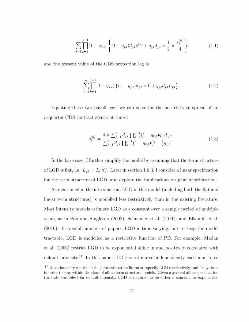
n
j1
j1¹k1
p1 qk,tq#p1 qj,tqdj,tspnq qj,tdj,t 1
2 s
pnqt
4
+(1.1)
and the present value of the CDS protection leg is
n
j1
j1¹k1
p1 qk,tq p1 qj,tqdj,t 0 qj,tdj,tLj,t
(. (1.2)
Equating these two payoff legs, we can solve for the no arbitrage spread of an
n-quarter CDS contract struck at time t
spnqt 4°n
j1 dj,t±j1
k1p1 qk,tqqj,tLj,t°nj1 dj,t
±j1k1p1 qk,tqp1 1
2qj,tq
. (1.3)
In the base case, I further simplify the model by assuming that the term structure
of LGD is flat, i.e. Lj,t Lt @j. Later in section 1.6.3, I consider a linear specification
for the term structure of LGD, and explore the implications on joint identification.
As mentioned in the introduction, LGD in this model (including both the flat and
linear term structures) is modelled less restrictively than in the existing literature.
Most intensity models estimate LGD as a constant over a sample period of multiple
years, as in Pan and Singleton (2008), Schneider et al. (2011), and Elkamhi et al.
(2010). In a small number of papers, LGD is time-varying, but to keep the model
tractable, LGD is modelled as a restrictive function of PD. For example, Madan
et al. (2006) restrict LGD to be exponential affine in and positively correlated with
default intensity.17 In this paper, LGD is estimated independently each month, so
17 Most intensity models in the joint estimation literature specify LGD restrictively, and likely do soin order to stay within the class of affine term structure models. Given a general affine specification(in state variables) for default intensity, LGD is required to be either a constant or exponential
12

even though the model lacks dynamic features, we still obtain a sequence of monthly
estimates of LGD. Additionally, there are no functional restrictions between LGD
and PD. The obvious drawback is that we lose any efficiency gains that would be
achieved if the relationship between LGD and PD were correctly specified.
Under the flat term-structure assumption for LGD, the CDS premium expression
is simplified to
spnqt L
4°nj1 dj,t
±j1k1p1 qk,tqqj,t°n
j1 dj,t±j1
k1p1 qk,tqp1 12qj,tq
. (1.4)
In this pricing equation (1.4), there are n 1 unknowns: qj,t for j 1, . . . , n,
which map out quarterly points on the forward PD curve, and Lt, the expected
loss given default. In my analysis, there are n 40 quarters in total, so to make
estimation feasible, I reduce the dimensionality of the model by adopting a family of
flexibly-shaped curves f for the default probability term-structure, i.e. qj,t fpj; βtq.
1.3.2 A factor model for the term structure of default probabilities
Determining a suitable model for the forward default curve is difficult since the
default curve is not observed, even ex post. However, I can construct a set of “proxy”
PD curves for the unobserved PD term structures, conditional on a flat term structure
for LGD (as assumed in this model). Then I can find a factor model that captures
most of the variation of the proxy curves.
Since construction of the proxy curves requires a fixed value of LGD, yet the
resulting curves may be sensitive to the particular choice, I consider various levels
affine in the default intensity process. Exceptions are Christensen (2005) and Christensen (2007),where both default intensity and LGD are affine in state variables, which leads to a quadratic termstructure model for CDS prices. The quadratic term structure model is the highest order model forwhich closed form solutions exist. Elkamhi et al. (2010) also use a quadratic term structure modelfor CDS prices, but they allow default intensity to be quadratic in latent factors, and then mustmodel LGD as a constant to ensure close-form solutions for CDS prices.
13

for the LGD term structure, 0.1, 0.2, 0.4, 0.6, 0.8, 1, and construct a set of
proxy curves for each value of LGD. So, for each value of LGD, assuming a flat
default probability between consecutive CDS maturities, I “strip” each daily CDS
price curve from lowest to highest maturity to get a step function with 8 steps as an
approximate forward PD curve. See Figure A.1 in the appendix for an example for
CDS data from one day.18 Then, for each fixed value of LGD, I conduct principle
components analysis on the set of 8-dimensional vectors that represent daily implied
forward default probability curves. The analysis is conducted separately for each of
the 30 firms and on the pooled set of implied PD curves (after demeaning for each
issuer) across all assets. Figure 1.2 presents the first three principal components for
the pooled set of PD curves for all six values of LGD. For each fixed value of LGD,
95% to 98% of all variation in the pooled PD curves is captured by the first three
components. Further, the components visually resemble level, slope and curvature
loadings. These results suggest that using a 3-factor “level-slope-curvature” model
for the forward default probability curve is a good approximation.
1.3.3 Nelson-Siegel curves: a level-slope-curvature model
Based on the results of the principal component analysis, I propose modelling the
forward default probability term structure qj,t using Nelson-Siegel curves, which are
a family of curves composed of a linear combination of three components resembling
level, slope, and curvature.
Equation (1.5) presents the form of the Nelson-Siegel curve used in this paper,
which is the Diebold and Li (2006) reparameterization of the original form that
18 The 8-step default probability curve assumes constant forward default proba-bility per quarter over the following time intervals (units in years) whose end-points correspond to CDS contract maturities: pt, t 0.5s,pt 0.5, t 1s,pt 1, t 2s,pt 2, t 3s,pt 3, t 4s,pt 4, t 5s,pt 5, t 7s,pt 7, t 10s . Resulting proxy PD curveswith values not in the p0, 1s interval are discarded from the PCA.
14

Nelson and Siegel (1987) propose to fit U.S. government yield curves. The three β
coefficients determine the weights of each component, while the fourth parameter
λ determines the rate of decay of the exponentials in the function, which directly
relates to the shape of the slope component and the location of the “hump” in the
curvature component. See Figure 1.3 for an illustration of the three Nelson-Siegel
curve components.
fpj;βtq β1t β2t1 eλj
λj β3t
1 eλj
λj eλj
(1.5)
Nelson-Siegel curves have been used extensively in research and in practice, in-
cluding by central banks.19 They are noted for their parsimony and ability to match
the many shapes of observed yield curves, including flat, upward or downward sloping
with varying convexity, humped, and mildly S-shaped.
As mentioned above, the λ parameter in the Nelson-Siegel curve determines the
exact shape of the slope and curvature components. For larger values of λ, the slope
component decays slower and the curvature component reaches its maximum later.
In the yield curve literature, λ is often fixed to simplify yield curve estimation to
OLS. Nonlinear methods can be used to estimate a free λ; Nelson and Siegel (1987)
employ a grid search over λ, but the estimates are unstable over time, and Annaert
et al. (2013) caution that for certain values of λ, there is a high degree of collinearity
among the 3 components.
In this application, the CDS pricing equation is already nonlinear, but to avoid
adding an additional layer of nonlinearities, I fix λ guided by the results of the prin-
cipal components analysis. In the pooled PCA results, the estimated third principle
component (“curvature”) has a pronounced peak at the 5th step, which is centered
19 See Annaert et al. (2013) for discussion.
15

at the 3.5 year maturity (see Figure 1.2). Therefore, I fix λ 0.1281 so the hump of
the third component is at 3.5 years. In Section 1.6.1, I also estimate the model for
other values of λ as a robustness check, and the main conclusions of my analysis are
unchanged. This value of λ is somewhat similar to the value used in Diebold and
Li (2006), who choose λ to locate the maximum of the curvature component at 2.5
years because 2-3 year maturities are typical for humps and troughs in yield curves
in the literature.
This model abstracts from risk factors (unrelated to issuer default) such as illiq-
uidity (as mentioned in section 1.2.1, counterparty and contagion risk. Counterparty
risk is the risk to each party of the contract that the other will not be able to fulfill
their contractual obligations. Contagion (see Bai et al. (2013)) is the risk in credit
markets, distinct from default event risk, that default of systemically important firms
will cause a contemporaneous drop in the market portfolio. Bai et al. (2013) show
that all but a few basis points of credit spreads that attributed to the risk premium
on default probability in standard (doubly stochastic) intensity models is actually
contagion risk premium. In this model, these other risk premia are subsumed into
the estimates for risk neutral default probability and LGD. This is the standard
approach in the joint estimation literature because accounting for these two other
effects can be very complicated, and generally requires model extensions and addi-
tional data. It is difficult to say how illiquidity and counterparty risk premia will be
divided between risk neutral LGD or risk neutral probability of default. However,
contagion risk will likely be soaked up in the risk neutral default probability esti-
mates because in accordance with theoretical contagion models, only the likelihood
of default probability is directly affected through contagion channels: the probabil-
ity that a given firms will default increases when a systematically important firm
defaults, and there is no direct impact on recovery rates.
16

1.3.4 Joint Identification of Default Probabilities and Loss Given Default
As suggested in Pan and Singleton (2008), when LGD is modelled as the fractional
loss of bond face value given default, identification of both probability of default and
loss given default can possibly be achieved by exploiting both short and long term
CDS contracts because their prices are affected differently by the two components.
Pan and Singleton investigate and confirm the effectiveness of this identification
strategy using simulated data under a model with log-normal default intensity and
constant LGD. However, in the model used in the analysis below, it is easy to see
that there is a subset in the parameter space for which the model is not identified.
When the forward probability of default has a flat term structure, i.e. qj,t qt, then
the expression for the CDS price reduces to:
spnqt Lt
4°nj1 dj,t
±j1k1p1 qtqqt°n
j1 dj,t±j1
k1p1 qtqp1 12qtq
Ltqt
1 12qt
for n P N ; (1.6)
and it is apparent that Lt and qt are not point identified. However, as mentioned
in the introduction, it is interesting to point out that the identification issue here is
somewhat different than that of most applications in the weak-identification litera-
ture because, even in the problematic region in the parameter space, the nonlinear
function of Lt and qt on the right-hand side of Equation (1.6) is identified, which
restricts the values of Lt and qt to a set that is smaller than the logical range from
0 and 1 for each, so the model is set (or partially) identified.20 Furthermore, when
20 Intuitively, it is also easy to understand why the model is not point-identified in this region. Anon-flat CDS term structure contains different information about LGD and PD at each maturitypoint on the curve, so identification is generated by this information. When the term structure ofboth LGD and PD are flat, then the CDS term structure is flat, and additional maturity pointsbeyond the shortest one do not add any additional information, so we cannot distinguish therespective contributions of LGD and PD to the CDS price using information from only one maturity
point. However, set-identification comes from the fact that a certain level for the CDS spread spnqt
will guarantee that PD and LGD cannot be too low. The identified sets of pLt, qtq are decreasing
17

the PD curve is close to this non-identified region, the model is weakly identified: a
criterion function such as standard GMM or nonlinear least squares is relatively flat
with respect to Lt and β1t, so standard asymptotics (and standard t and QLR tests)
do not provide good approximations and are thus invalid.
Under the Nelson-Siegel parameterization, the non-identified region (or rather,
set-identified region) is characterized by β2t β3t 0, and since then qt β1t, the
subvector pLt, β1tq is not point-identified.
Also, it is worth noting that this weakly identified region nests the case when
default probabilities are very low, i.e. β1t, β2t and β3t are close to 0, a setting
in which other papers report having estimation or identification problems. In this
setting, suppose all qj,t η (a small number), so 1 qj,t 1 and 1 12qj,t 1. Then,
spnqt 4Lt
°nj1 dj,tη°nj1 dj,t
4Ltη, and thus Lt and η are not point identified.
1.4 Robust Inference under Weak Identification
In this section, I describe the weak-identification robust econometric tools that are
used in this paper, and I describe how these theoretical results can be used to con-
struct confidence sets for LGD.
1.4.1 S-test robust to weak identification
I treat observed CDS spreads as noisy realizations of the true price:
spnqit Ltgpβ1t, β2t, β3t;nqεit hpLt,βt;nqεit, for all days i in month t. (1.7)
If the model were globally identified, nonlinear least squares would be a straight-
forward choice for the estimation method. However, as described in the previous
in size (in a nested sense) with the level of st.
18

section, standard tests are not reliable in settings with weak identification, and ro-
bust estimation methods should be used instead.
Since the development of GMM in Hansen (1982), many papers have studied
GMM under nonstandard conditions, with weak identification attracting considerable
attention. Inference for general nonlinear models under weak identification is not
as extensive as the literature for robust linear instrumental variables estimation,
but under the weak instrumental variables framework in nonlinear GMM, Stock and
Wright (2000) derive the asymptotic distribution for the CUGMM objective function
under very weak conditions, and estimate robust confidence intervals for the CRRA
risk aversion coefficient in the consumption CAPM, which is weakly identified in
the model Euler equations. Even though the weak identification in this model is
not equivalent to that of the weak IV setting, the CUGMM results in Stock and
Wright are sufficiently general that I can borrow the same methodology to construct
confidence sets for LGD that are robust to weak identification.
To employ the methodology, the nonlinear least squares problem is recast in the
GMM framework (as minimum distance estimation). From here onwards, I suppress
the t subscripts for brevity, but it is understood that the model is estimated for
each month t using the pooled daily term structure spreads from that month. Let
θ pL,βq pL, β1, β2, β3q be the parameters of the model, and take the score
function of the least squares problem as the estimating equations:
φipθq φipθ; sq spnqi hpθ;nq
Bhpθ;nqBθ . (1.8)
Further, I define the standardized moment ΨNpθq N 12
°Ni1 rφipθq Eφipθqs
and its asymptotic variance, Ωpθq limNÑ8EΨNpθqΨNpθq1.
19

Then, the standard CUGMM objective function is
ScNpθq N 1
2
N
i1
φipθq1WNpθq
N 1
2
N
i1
φipθq, (1.9)
where WNpθq is an Opp1q positive definite 4 4 weighting matrix that is a function
of θ.
Suppose θ0 pL0,β0q are the true parameters of the model. The result I use
from Stock and Wright only requires the weak assumptions that the GMM moment
condition obeys the central limit theorem locally at θ0, i.e. ΨNpθ0q dÑ Np0,Ωpθ0qq,21
and that the weighting matrix used is consistent for the inverse of the asymptotic
variance of the standardized moment at θ0, i.e. WNpθ0q pÑ Ωpθ0q1. Under these
assumptions, Theorem 2 in Stock and Wright shows that ScNpθ0q dÑ χ24.
From this result, one can obtain an asymptotic level-α confidence set for θ, called
S-sets in Stock and Wright (2000), by inverting the CUGMM objection function
surface, that is
Cθ,α θ|ScNpθq ¤ χ2
4p1 αq( , (1.10)
where χ24p1 αq is the 100p1 αq% critical value of the χ2
4 distribution. However,
constructing Cθ empirically involves extensive computation; specifically, ScNpθq must
be evaluated over a very fine grid of values of θ spanning the 4-dimensional parameter
space. Instead, given our main focus is estimating LGD, we use a result similar to
Theorem 3 in Stock and Wright, which allows for confidence sets of a subset of the
parameters.22
21 Among other scenarios (structural breaks, existence of higher moments, etc), this assumptionprecludes the sequence of moment conditions from being integrated of order one or higher, whichis satisfied in this application.
22 The relationship between the strongly identified pβ2, β3q and weakly identified pL, β1q parametersin this CDS model is not characterized in the exact manner of Assumption C of Stock and Wright
20

Under the two assumptions on the GMM moments and weighting matrix, we get
that the profile CUGMM objective function evaluated at the true LGD value L0 con-
verges in distribution to a chi-square distribution, i.e. ScT pLq ScT pL0, βpL0qq dÑχ2
1, where βpLq argminβScT pL,βq. This result allows us to obtain asymp-
totic level-α confidence sets for L by inverting the profile S-function, i.e., the set
CL,α !L|ScT pL, βpLqq ¤ χ2
1p1 αq). Equivalently, this procedure can be thought
of a test (called an S-test) of model specification and parameter identification: the
model with parameter value L P p0, 1s is rejected at the p1αq confidence level if the
S-function evaluated at L is greater than the chi-square critical value. If all values
in p0, 1s are rejected, then the model has been rejected entirely.
Note that while the computational time is drastically reduced compared to esti-
mating confidence sets for θ, the procedure, which will be described in further detail
in the next subsection, still requires mapping out the profile-S curve for many values
of L, and each point on this curve is obtained from a nonlinear optimization over β.
The asymptotic result from which the S-sets are developed relies jointly on identi-
fication of the true parameter θ0 and validity of the GMM orthogonality conditions.
Therefore, as alluded to above, the confidence set consists of parameter values at
which the joint hypothesis that θ θ0 and Erφtpθ; sqs 0 is unable to be rejected.
In contrast, conventional tests (Wald, LR) operate under the assumption that the
orthogonality conditions hold, and are only a test of parameter identification.23
This feature of the S-sets is valuable as it can detect a misspecified model by
(2000). Also, note that in the weak IV model studied in Stock and Wright (2000), Theorem 3 doesnot allow for asymptotically valid confidence sets for a subset of the weakly identified parameters.However, Theorem 3 holds since when L L0, pβ1, β2, β3q are well-identified (and thus consistentlyestimated), which is the general purpose of requiring Assumption C. This hold because a function ofLandβ1 are identified, so fixing L at the true value allows for consistent estimation of the remainingparameters.
23 As discussed in Stock and Wright, under conventional asymptotics (not in the presence of weak-identification), ScT pθ0q is asymptotically the sum of the Likelihood Ratio (LR) statistic testingθ θ0 and Hansen’s (1982) J statistic testing the over-identifying conditions.
21

rejecting the entire parameter space. However, the trade off is that non-empty confi-
dence sets require some care in interpretation that is not necessary with conventional
tests. If an S-set is nonempty, there are two possibilities: either the model is correctly
specified and parameter estimates are given by the S-set, or the model is misspeci-
fied, but, for the values in the S-set, the test lacks power to reject the model. Very
large S-sets suggest that there is little evidence to distinguish between parameter
values, but small confidence sets are more difficult to interpret; they could reflect a
correctly specified and precisely estimated model, or a misspecified model that the
test was not powerful enough to reject for a small set of parameter values. There is
no solution to this problem, which is faced by all tests of this type, but in the results
section, in addition to running the 0.05-level test, I also consider the more powerful
0.10-level test and find that results do not change much.
1.4.2 Estimation procedure for confidence sets for LGD
As described in Section 1.3, I assume that CDS spreads from each calendar month
are generated from the same data-generating process, so the model can be estimated
independently each month using the available panel of observed CDS spreads. Gener-
ally, this is a reasonable assumption since CDS spread dynamics are very slow-moving
as shown in Section 1.2.2, but it is possible that for some months, the constant pa-
rameter assumption is not a good approximation. For example, we could envision a
news shock in the middle of some month that causes sudden changes in beliefs about
a firm’s credit. However, the important point is that the S-sets are valid regardless of
whether the assumption holds because they jointly test parameter identification and
model specification. Thus, if the constant model assumption were false, the model
would be rejected for all values of LGD, i.e. S-sets would be empty.24
24 As a robustness check, I also assume a constant CDS model over longer and shorter timeperiods (semi-monthly and quarterly) and check for changes in estimated confidence sets. The
22

There are 2972 issuer-months in total, and for each issuer-month, the model is es-
timated using approximately 176 (approximately 22 days8 contracts/day) pooled
individual CDS spreads. The weighting matrix form used in the CUGMM objec-
tive function is the inverse heteroskedasticity robust asymptotic variance WT pθq !T1
°Tt1
φtpθq φpθq φtpθq φpθq1)1
. As a robustness check for contract ef-
fects, I also consider the clustered variance estimator to account for maturity point
effects, and a Newey-West HAC-style estimator to account for serial correlation.25
For each month, a confidence set for LGD can be obtained by evaluating the
profile S-function ScT pL, βpLqq for a grid of values L for LGD and comparing the re-
sulting values with a chi-square critical value. If the profile S-function evaluated at L
is less than the critical value, then L is in the confidence set. Note that the confidence
set may be disjoint. As an initial grid for LGD, I use L t0.01, 0.02, ...0.98, 0.99, 1u.For each value of L, ScT pL,βq is minimized over β, with parameters constrained so
that default probability curves are in [0,1].26
In the second stage, I evaluate ScT pL, βpLqq on a finer grid (grid space of 0.001
instead of 0.01 as in the original grid L) around the values of L where ScT pL, βpLq)attains a local minima or is close to the chi-square critical value. Respectively, adding
detailed results are presented in the appendix, but generally there are two contrasting effects fromchanging the data aggregation period: using less data (using CDS data over a shorter period)will reduce the power of the test, but on the other hand, a longer time period is more likely tocompromise the assumption of the constant DGP, leading to either larger confidence sets due to“extra noise” in the data or empty confidence sets if there is enough power to outright reject themodel.
25 (Results will be updated when available, please visit my website http://sites.duke.edu/
lilyyliu for the latest version.)
26 Due to the nonlinearity of the profile S-function, I start the optimization procedure fromaround 1000 initial values from the compact parameter space for β. These values were not sampleduniformly from the entire parameter space. Instead, more “reasonable” regions (those mapping tolower default probabilities) were sampled more frequently. In addition, if the profile S-curve (as afunction of L) has upward spikes in it, indicating that the first round of optimization stopped ata local minima, the optimization procedure for those values of L was repeated using initial valuessimilar to the β estimates from nearby values of L. This was repeated until the spikes in theprofile-objective curve were resolved.
23

these two finer grids reduce the chance of incorrectly rejecting the model (finding an
empty S-set) due to errors from LGD grid discreteness and allows estimation of the
S-set end-points to be precise to 0.1%.
1.4.3 Examples of Profile S-functions and S-sets
Before presenting the main results of the paper, I plot, in Figure 1.4, concentrated
S-functions from 4 months to illustrate S-sets constructed from actual data. In
addition, I describe how the confidence sets from this method can look different
from conventional confidence intervals from likelihood ratio (LR) and Wald tests. A
confidence set from a standard Wald test is generally a symmetric interval around the
point estimate, and confidence sets from both LR and Wald tests are not empty and
not disjoint by construction. The two top subplots show typical shapes of the profile
S-curve that yield small and very large confidence sets. The confidence sets are not
symmetric around the CUGMM point estimate (CUE), where the profile S-function
reaches its minima. In addition, the bottom left subplot shows an issuer-month
for which an empty confidence set is estimated. The bottom right subplot shows a
disjoint confidence set. Disjoint S-sets are observed for 210 out of 2972 issuer-months
in this sample, and almost all of them cover a large portion of the (0,1] parameter
space. Finally, we observe that the profile S-function diverges for very small values
of LGD, which is expected since the CDS price is undefined when LGD equals zero.
1.5 Empirical Results from Joint Estimation
In this section, I present the main results. In particular, I describe the estimated
confidence sets for LGD, and address the two main questions of the paper: can LGD
be precisely estimated when jointly estimated with LGD in this term structure model,
and if so, is 60% a good estimate for LGD? In addition, I explore the differences
24

in the results across issuers and over the sample period, and investigate whether
characteristics of the monthly CDS data affect how precisely LGD is estimated.
Finally, I study the implied default curves that are jointly estimated with LGD, and
discuss the implications on credit risk premia.
1.5.1 Confidence Set Lengths and Locations
Here, I present a summary of the sizes and location (on the (0,1] parameter space) of
the 2972 estimated monthly confidence sets for LGD and address a main question of
whether LGD can be jointly estimated alongside default probabilities, which in effect
is asking how large are the confidence sets for LGD? If the estimated confidence sets
are all large subsets of the total parameter space (0,1], then it implies that many
combinations of LGD and PD are indistinguishable in their ability to fit the spread
data, and hence, we gain little information about the true value of risk-neutral LGD.
In Table 1.2, I divide the 2972 S-sets into bins based on their size, and report the
proportion of confidence sets in each bin. I find that the confidence sets for LGD are
concentrated in the smallest and largest bins. For 38.2% of issuer-months, LGD is
estimated very precisely, with confidence sets less than 0.10 in length. Another 5.3%
of issuer-months have confidence sets between 0.10 and 0.20 in length. However, an
almost equally large fraction (32.6%) of issuer-months have estimated confidence sets
that are very large, greater than 0.80 in length, which indicates an almost complete
lack of information in the data to distinguish between the roles of LGD and PD
in the cross-sectional model. Also, it is interesting to note that there are very few
issuer-months in the mid-sized confidence set bins – only 9.8% of confidence sets are
between 0.20 and 0.80 in length.
In addition, 14.2% of the confidence sets are empty, meaning that the model is
rejected for all values of LGD at the 0.05 level. Rejection of the model could be due
25
to one or more of the following: the Nelson-Siegel curve parameterization for PD is
incorrect, the flat term-structure for LGD is a poor fit, or the constant parameter
assumption failed for the month in question.27
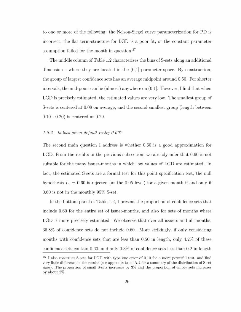
The middle column of Table 1.2 characterizes the bins of S-sets along an additional
dimension – where they are located in the (0,1] parameter space. By construction,
the group of largest confidence sets has an average midpoint around 0.50. For shorter
intervals, the mid-point can lie (almost) anywhere on (0,1]. However, I find that when
LGD is precisely estimated, the estimated values are very low. The smallest group of
S-sets is centered at 0.08 on average, and the second smallest group (length between
0.10 - 0.20) is centered at 0.29.
1.5.2 Is loss given default really 0.60?
The second main question I address is whether 0.60 is a good approximation for
LGD. From the results in the previous subsection, we already infer that 0.60 is not
suitable for the many issuer-months in which low values of LGD are estimated. In
fact, the estimated S-sets are a formal test for this point specification test; the null
hypothesis L0 0.60 is rejected (at the 0.05 level) for a given month if and only if
0.60 is not in the monthly 95% S-set.
In the bottom panel of Table 1.2, I present the proportion of confidence sets that
include 0.60 for the entire set of issuer-months, and also for sets of months where
LGD is more precisely estimated. We observe that over all issuers and all months,
36.8% of confidence sets do not include 0.60. More strikingly, if only considering
months with confidence sets that are less than 0.50 in length, only 4.2% of these
confidence sets contain 0.60, and only 0.3% of confidence sets less than 0.2 in length
27 I also construct S-sets for LGD with type one error of 0.10 for a more powerful test, and findvery little difference in the results (see appendix table A.2 for a summary of the distribution of S-setsizes). The proportion of small S-sets increases by 3% and the proportion of empty sets increasesby about 2%.
26

include the value 0.60. Thus we conclude that in the months that LGD is precisely
estimated, 0.60 is rejected as a value for risk neutral LGD. However, these results do
not rule out that 0.60 is an appropriate value for LGD in the approximately one-third
of issuer-months that have very large LGD confidence sets.
1.5.3 Confidence sets across reference entities and over time
The above analysis focuses on characterizing the aggregate collection of estimated
confidence sets, but we are also interested in discovering heterogeneity in the results
across firms and over time. The top two subplots of Figure 1.5 summarize the dis-
tribution of confidence set sizes for each of the 30 reference entities. The top panel
plots the proportion of S-sets that are less than 0.1 in length and the average S-set
center of these small sets, per firm. The middle panel plots the proportion of large
S-sets (length greater than 0.6), and the proportion of empty confidence sets (to
make the plot easier to read, the firms have been ordered by the proportion of small
confidence sets). We see that the proportion varies substantially across firms from
61% (Whirlpool, WHR) to only 17% (American Express, AXP). We also see some
variation in the average midpoints of these small S-sets; average midpoints lie be-
tween 0.03 (General Electric Capital, GEc) and 0.18 (Tenet Healthcare, THC). These
results lead us to ask whether there are variables that can explain the differences in
confidence set size and in the estimated level of LGD when precisely estimated. We
investigate the former in section 1.5.4 and the latter in section 1.5.7 after describing
the estimates for the forward default probability curve.
Additionally, we can investigate if 0.60 is a better estimate for LGD for certain
reference entities. The bottom panel of Figure 1.5 plots the proportion of confidence
sets that include 0.60, keeping the same order of firms as in the top panel. This
proportion ranges from 22% for Sabre Holdings (TSG) to 57% for American Express
27

(AXP). In addition, the bottom panel also presents the proportions of confidence sets
with length less than 0.5 or less than 0.2 that include the value 0.60. The latter set
of proportions ranges from 0 to 7%, which further illustrates that 0.60 is generally
only in large S-sets, i.e., when there is insufficient information in the data to jointly
estimate LGD and PD.
In addition to tabulating summaries of the confidence sets for individual assets,
we can plot the S-sets over time, per firm. Figure 1.6 plots the confidence sets for
two representative firms, Xerox and Goodyear Tire. Both plots show a pattern that
is present for almost all issuers: large confidence sets are concentrated during the
financial crisis period from late 2007 through 2009, while the periods before and after
have fewer large confidence sets.
To explore this further, I divide the 100 month sample period into three sub-
periods of approximately equal length, and in Table 1.3, I reproduce the confidence
set summaries as in Table 1.2 for each sub-period. Period 1 runs from Jan 2004-Sep
2006 (33 months), period 2 runs from Nov 2006-Jun 2009 (33 months), and period 3
runs from Jul 2009-Apr 2012 (34 months). Note that period 3 incidentally coincides
almost exactly with the post CDS Big Bang era.28 Across these three sub-periods,
the estimated LGD S-sets are quite different. In the earliest and latest parts of the
sample, Jan 2004-Sept 2006 and July 2009-April 2012, over half of the issuer-months
have over confidence sets smaller than 0.10, and around 20% of confidence sets are
larger than 0.8. In terms of empty confidence sets, the latest subperiod has the
fewest at only 4.6%, while the earliest subperiod has the largest proportion at 7.6%,
however, both of these values are close to the specified level of the test. The middle
period, which contains the recent financial crisis, contains the smallest proportion of
precisely estimated confidence sets for LGD: 39% of the monthly confidence sets are
28 The CDS Big Bang was announced in April 2009, and policies were implemented 2-3 monthslater.
28

over 0.8 in length, and only 29% of months have length less than 0.1. So the main
difference observed in the three subsamples is that in the middle period, 20% of the
confidence sets get redistributed from the less-than 0.1 bin to the greater-than 0.8
bin.
A final comment on the confidence sets over time: it is observed that the small
confidence intervals are usually estimated clustered together; however, there are nu-
merous cases when a string of small monthly confidence intervals, roughly estimated
at the same level, is interrupted by one or several large confidence intervals that span
almost the entire parameter space (for example Jan-May 2005 for Xerox in Figure
1.6). I stress that this does not necessarily mean that risk neutral LGD jumped
from around 0.10 to 0.90 (or even to the midpoint of the large confidence set) and
then back over the span of 1 month. This sequence of confidence intervals is also
consistent with the true implied LGD staying steady at 0.10 over all the months, as
0.10 is in the confidence set for all three months. The large S-set is just a conse-
quence of the data containing limited information that month, so virtually no values
in the LGD parameter space could be rejected. In this next subsection, I will explore
whether characteristics of the CDS spread data can explain differences in sizes of the
confidence sets.
1.5.4 Effects of CDS data characteristics on Confidence Set Size
In this section, I summarize how three characteristics of monthly CDS data are
related to the size of LGD confidence sets, using a fractional-response general linear
regression (with logit link function) by regressing the size of monthly confidence sets
on explanatory variables constructed from monthly CDS data.
In section 1.3.4, it is shown that when the PD term structure is flat, the cross
sectional model is not identified. Maintaining the model assumption that the LGD
29

term structure is flat, flat PD term structure implies a theoretical CDS term structure
that is also flat. Thus, I investigate whether LGD S-sets are larger for months with
flatter CDS term structures by including in the regression a measure of CDS term
structure “flatness” – the absolute value of the slope (the 10-year spread minus the
6-month spread) plus the absolute value of the curvature (2 times the 5-year spread
minus both the 6-month and 10-year spreads). In addition, noisy data caused by large
errors diminishes the test’s ability to extract information about the true model, so I
also include a measure of noise variance – the within month coefficient of variation
of 5-year spreads. The coefficient of variation is defined as the sample standard
deviation divided by the sample mean, so more precisely it is a noise-to-signal ratio.
Finally, I also include the mean of the 5-year spreads as an explanatory variable,
which can be viewed as a proxy for level of credit distress of the reference entity,
and is also related to identification, because as noted in section 1.3.4, if spreads are
high when PD term structure is flat, then the identified set for pLt, qtq is smaller
than when spreads are low. Also, point identification may be threatened when CDS
spreads are near zero.29,30
The regression results are reported in Table 1.4.31 The regression is conducted
over the full sample and separately for each subperiod. For each sample period,
29 An alternate regression specification using the standard deviation of 5-year spreads (unstan-dardized) as the “noise” variable produces similar results, however the three explanatory variablesare highly collinear, whereas the coefficient of variation is almost uncorrelated with both average5-year CDS spread and term-structure flatness. The average 5-year spread and the term structureflatness measure have a sample correlation of 0.60 over all firms and all months. In addition, thecoefficient of variation measure is more comparable in level across all firms, whereas the averagestandard deviation across firms is substantially varied.
30 The estimates of β2 and β3 could be used to used as explanatory variables, however I choose toonly use variables that can be directly measured from the CDS spreads before any estimation takesplace.
31 I stress that this regression is merely a summary tool for exploring how characteristics of monthlyCDS spreads affect S-set size. It is not proposed as a model for the dependent variable (S-setlength), nor is this variable truly intended to be interpreted as a random variable. It follows thatthe standard errors are not interpretable in the regular sense, but they are reported as they still doprovide some indication of how strong the regression association is.
30

explanatory variables have a strong relationship with the confidence set length, and
have signs in the expected direction. When the CDS term structure is less flat
(i.e., the “flatness” variable takes a higher value), LGD is more precisely estimated
(smaller S-sets). Also, a higher coefficient of variation, a proxy for noisier data,
is associated with a larger confidence set, which is also expected since information
in the data is more heavily contaminated by noise. Finally, the level of the 5-year
CDS has a positive effect on confidence set length. In the full sample regression, it
is possible that the significance of the coefficient estimates are driven by the large
differences in CDS spread behavior during the “financial crisis” period and in the rest
of the months. However, the results are robust for all three subperiods, as shown in
Table 1.4, and Periods 1 and Periods 3 do not overlap with the financial crisis, so the
significance of these three credit spread factors is not only driven by the disparate
financial crisis period.
1.5.5 Estimated default probability term structure
As explained in Section 1.4.1, I do not construct confidence sets for the full parameter
vector pL, β1, β2, β3q in this paper due to computational burden, however, we can still
study the (point) estimated PD term structures given a fixed value of L, i.e. the PD
term structure implied by βpLq argminβScT pL, βq.32 In particular, I am interested
in comparing the estimated PD term structure corresponding to LGD fixed at 0.6,
βp0.60q (which I will refer to as conventional PD) to the PD term structure at the
CUGMM point estimate (CUE), βpLcueq (referred to as estimated PD).
I limit this analysis to months when LGD is precisely estimated (S-set length
is less than 0.1), which is the case for 1335 issuer-months out of the total 2972.
32 Note that the values of LGD in the S-sets and their corresponding estimated PD term structures,i.e. tpL, βpLqq : L P CLu, represent estimated models that are not rejected under the S-test with
level 0.05, however the set of β estimates tβpLq : L P CLu do not make up a correctly sized(asymptotically) confidence set for pβ1, β2, β3q.
31

Summaries of the average PD term structures are presented in Table 1.5. The average
point estimates of LGD are 0.073 for investment grade issuers and 0.113 for high yield
issuers, which are about 8.3 and 5.3 times lower than 0.60, respectively.33 I find that
for the months with small confidence sets, estimated PD is, on average, 10.9 times
higher than conventional PD. Notably, the long-maturity end of the estimated PD
curve ranges from 5-30 times higher than that of the conventional. Table 1.5 further
distinguishes between investment grade and high yield reference entities, and presents
average values of estimated and conventional forward default probabilities and the
average ratio of estimated to conventional PD for four maturity points. On average,
the term structure of estimated PD is 12-15 times higher than that of conventional
PD for investment grade entities, and 6-9 times higher for high yield entities. I
also include, in Table 1.5, the average cumulative default probability at 4 points
along the term structure, denoted by qj,t, and I note that the ratio between the
estimated cumulative PD and conventional cumulative PD decreases as the maturity
increases, i.e., as default probabilities are compounded. However, even at 10 years,
the estimated cumulative default rate is 5.0 times higher for investment grade issuers
and 2.7 times higher for high yield issuers, a substantial magnitude of difference.
Therefore, for the months where LGD is precisely estimated, default probabilities
are hugely biased when LGD is fixed at 0.60.
1.5.6 Discussion of risk premia implications
Existing papers that quantify risk premium in credit spreads use models with loss
given default fixed exogenously, so in addition to possibly estimating distorted values,
the entire premium (excess returns) in CDS is counted as compensation for default
33 Recall that on average, the small confidence sets are centered at a value 6-8 times lower than0.60 (see Table 1.2; the average LGD CUE are usually slightly lower these confidence set midpointsbecause the small confidence sets are slightly asymmetrical around the point estimate.
32

probability risk. For example, Driessen (2005) and Berndt et al. (2008) use the
ratio of risk-neutral to actual default probabilities as a measure of the proportional
premium for bearing default risk.34 They fix LGD at 0.60 and approximately 0.75,
respectively, and estimate the risk premium ratio of default intensities to be around
2-4 for U.S. corporates.
However, there is uncertainty regarding loss given default as well, and an impor-
tant question that arises is whether risk in LGD is priced, or if the premium observed
in credit spreads is correctly attributed to the probability of default. In this paper,
I directly model and estimate risk neutral LGD and PD curves, and as such, this
model does not contain the machinery to extract risk premia or actual expectations
of default probabilities and loss given default. However, it is still sensible to discuss
what the estimates of risk-neutral LGD and probability of default imply for risk
premia, and any differences that arise when LGD is fixed exogenously. In addition,
the following analysis puts forth pertinent questions for future research.
In the previous subsection, it is clear that the ratio of default probabilities under
the estimated and conventional treatments for LGD change depending on what the
exact underlying probability is, i.e., forward probability or cumulative probability,
and the length of the period. To investigate how the magnitude of the risk premium
on default probabilities might change when LGD is estimated from the data, I com-
pute a simple default intensity loosely comparable to the default intensities studied in
Driessen (2005) and Berndt et al. (2008). I back out the default intensity associated
with the cumulative 10-year probability of default presented in Table 1.5, assuming
constant intensity over the 10-year period. These default intensities (average λq) are
listed in the right-most column of Table 1.5 along with the ratio between the implied
34 Berndt et al. (2008) gives the example that “if this ratio is 2.0 for a particular firm, date ormaturity, then market-based insurance of default would be priced at roughly twice the expecteddiscounted default loss.” Driessen (2005) studies credit risk using corporate bond data.
33

default intensities. This analysis shows that the ratio of the default intensities is 8.8
for IG firms and 5.3 for HY firms, meaning that, at least in this sample and given the
model of this paper, the ratio of risk-neutral to objective default intensity would be
8.8 or 5.3 times higher than if LGD were fixed exogenously at 0.60. So, in summary,
the risk premium on default probability is grossly understated if LGD is fixed at 0.60
rather than estimated.
A puzzle that now arises is that the risk premium on default probability is too
high to be reasonably explained by most standard models. A possible explanation
for the high values of risk neutral PD when LGD is jointly estimated is that a
large proportion of the risk premium should be attributed to contagion risk. The
firms selected for this study (firms listed in CDX indices) are very large firms whose
default is strongly associated with bad times for the market overall, and could cause
a contemporaneous negative drop in the market portfolio; see Bai et al. (2013) for a
model with this feature. If the study focused on smaller, systemically less important
firms, the risk premia may be smaller, though it is possible that the objective default
probabilities may be larger in the case of a smaller firm.
Regarding the implications for risk premia associated with LGD, as mentioned
above, the estimates of loss given default are much lower than the historical rate of
0.60, which leads to questioning if the risk premium on LGD is negative. A negative
risk premium for LGD is difficult to believe, as it implies that when the market
is in an overall bad state, default losses become less severe). This would be at
odds with financial theories and empirical evidence documenting decreased value of
firm collateral and increased fire-sales during times of financial distress, which cause
lower recovery rates than usual. However, estimates of LGD being around 0.10 is
not inconsistent with a positive risk premium for LGD, because both the estimated
risk neutral LGD in this paper, and the historical average 0.60 are not estimates of
34

the unconditional mean of LGD under the two different probability measures. Under
the objective measure, LGD is most likely not independent of default probabilities.
Instead, low LGD is probably associated with very low PD and vice versa. Then,
realized LGD in the historical data is more often drawn from the region of heavy
losses. Furthermore, the true conditional objective LGD could be very low in this
sample – less than 0.10, which would imply a positive risk premium for LGD. These
claims cannot be substantiated in this framework, but they can not be ruled out
either, and are a more plausible interpretation of the risk premium for LGD.
1.5.7 Firm characteristics and credit rating effects
In this section, I study whether firm characteristics are related to estimated levels
of LGD and PD using a two-equation panel regression. The LGD and PD mea-
sures, which are the two dependent variables in this regression, are the CUGMM
point estimate for loss given default Lcue, and the average (across maturities) quar-
terly forward default probability corresponding to Lcue, denoted as avgPDpLcueq °40j1 qjpβpLcueqq. I conduct this analysis on the full set of issuer-months with non-
empty confidence sets. However, for the largest confidence sets, there is very little
variation in the CUGMM point estimate for LGD, which is usually very close to 1.
These data points may act as highly influential “outliers”, or cause a nonlinear effect
in the data that cannot be accounted for using the (generalized) linear regression.
Thus, I also conduct the panel regression for the subsets of issuer-months where the
LGD confidence set is less than 0.7, 0.5, 0.2, or 0.1 in length to see whether results
change. For each of these five data subsamples, I estimate the LGD and PD equa-
tions jointly by stacking the equations. Since both dependent variables take values
between 0 and 1, I conduct a fractional response general linear model regression with
a logit link function.
35

The monthly measures of firm characteristics included in the analysis are leverage
(ratio of debt to book equity), realized variance of the firm equity price (a proxy for
the volatility of firm value), book-to-market ratio (B/M), firm size (log of market
capitalization), and credit rating. Following Papke and Wooldridge (2008), I also add
time averages (computed per firm) of each of the explanatory variables to control for
firm-level fixed effects.35 Monthly realized volatility is computed as the square root
of the sum of daily “close-to-close” squared returns, using price data from CRSP. All
other data used to construct the explanatory variables is sourced from Compustat.
Quarterly data items (such as those used to compute leverage and B/M) were as-
signed to the 3 calendar months spanning the quarter. Monthly Standard and Poor’s
credit ratings were converted to an ordinal number scale, where 1 is the highest rat-
ing. Data for privately held firms is not available on Compustat or CRSP, and thus
those firm-months were dropped from the analysis.
Firm leverage and firm value volatility are included in the regression because they
are the two sole determinants of credit spreads in the early structural credit model
of Merton (1974). In addition, previous studies have found that loss given default is
lower for firms in industries that naturally possess more tangible assets that can be
sold in the event of a bankruptcy, and firm leverage could reflect this information.
Book-to-market is included to see whether there is a relationship between the mar-
ket’s valuation of a firm (relative to it’s accounting value) and the market’s beliefs
about the firm’s credit risk.
The inclusion of credit rating as an explanatory variable may seem natural but
the expected relationships with the dependent variables are not completely straight-
forward. Credit ratings are a qualitative measure of how likely it is that a firm will
35 The time-series dimension is 100 in this setting, so firm-level fixed effects could probably beestimated directly by including a dummy variable for each group (and omitting the constant),however this involves adding a large number of constants, so I use the approach of Papke andWooldridge (2008) which was developed for large-N , small-T panels.
36

honor its debt obligations, implying a close relationship with objective probability
of default, but it is unclear if credit rating is related to the risk neutral counterpart.
Furthermore, the expected relationship between credit ratings and LGD is not clear,
because firms are not rated by how much they will fall short of their obligations if
they do default. However, if firms with higher default probabilities also have lower
recovery rates after default, we would observe a negative relationship between LGD
and credit quality.
Market capitalization is included to see if there is a relationship between size of a
firm and its default probability. Again, the expected relationship is not clear. On one
hand, we might expect smaller firms to have more credit risk, in the same manner
that “small” firms are shown to be riskier in the Fama-French three-factor model.
However, if large firms are more systemically important than small firms, then the
risk-premium on default probabilities, and thus risk-neutral default probability would
be higher. Ideally, we would want to study the relationships between firm size and
the objective default probability and firm size and risk premium separately (and on
a larger and more varied cross-section of firms), but unfortunately, this model setup
does not allow for any direct measures of risk premium.
The regression results are shown in Table 1.6.36 Most of the significant results
are for the PD equation; I find very few significant relationships for LGD. As ex-
pected, credit rating has a significantly positive (0.05-level) coefficient for PD in each
regression, meaning that as credit rating gets worse, the estimated average PD term
structure increases. Interestingly, firms with lower credit rating were found to have
lower LGD estimates, but this result only holds in the full sample, where lower credit
rating is highly correlated with times when the CDS spreads were noisier, and thus
the LGD confidence set are very large, and the point estimate approximately equals
36 In addition to the time-averaged variables, a constant (common to both equations) was includedbut is not reported in the table for brevity.
37

1. For all of the other samples that drop the largest confidence sets, there is no
significant relationship between credit rating and LGD.
Across all subsamples, leverage ratio and book-to-market ratio are not signifi-
cantly related to LGD or PD. Months with higher volatility see significantly higher
default probabilities, but are not related to the point estimate of LGD, except for
in the regression limited to confidence sets less than 0.1 in length, in which the co-
efficient is significantly negative. Market capitalization was not significant for LGD,
but all five regressions showed that firm size is negatively related to the default prob-
abilities. This result is analogous to the size premium in equity returns and deserves
further study.
1.6 Robustness Checks and Other Extensions
In this Section, I estimate variations of the base model to investigate the robustness of
results to model assumptions. First, I change the fixed values of λ to allow different
amounts of curvature in the Nelson-Siegel function. Secondly, I consider different
durations for the constant parameter assumption, or in other words, I estimate the
model on time periods shorter than and longer than one month, and check whether
results change.
In addition, I also investigate whether the model can be precisely estimated when
LGD is allowed a linear term structure.This extension on the model is not meant as a
literal check for model robustness, but are more intended to demonstrate that when
additional degrees of modelling freedom are allowed, confidence sets for LGD will
not pin down economically meaningful values for LGD (and thus PD). This actually
suggests that this non-time series approach to jointly estimating LGD and PD has
its shortcomings as well.
Finally, I provide a brief discussion of how the model can be applied to a larger
38

set of single-name CDS contracts, or augmented to include simple dynamics.
1.6.1 Alternate Nelson-Siegel Curves
Results in Section 1.5 are based on modelling default probability term structure using
Nelson-Siegel curves with λ fixed so that the hump of the Nelson-Siegel curvature
factor is located at 3.5 years (hereafter NS-3.5, for brevity). To check that results
are robust to the choice of λ, I consider two other sets of Nelson-Siegel curves with
λ fixed so the hump of the curvature factor is at 2.5 years or 4.5 years, abbreviated
NS-2.5 and NS-4.5, respectively. I reproduce the monthly confidence sets for LGD
for all thirty corporate issuers with the alternate Nelson-Siegel curves, and Table 1.7
presents the summaries of confidence set length and locations, comparable to Table
1.2.
I find very little change in the results. The estimated confidence sets under NS-
2.5 are in general centered slightly higher than the original set of results, while the
confidence sets under NS-4.5 are centered at the same level as the NS-3.5 results.
However, all three sets of confidence sets are centered at low values relative to the
entire (0,1] parameter space, and the value 0.60 is consistently not included in the
issuer-months where LGD is precisely estimated. Further, the model is rejected
much more often (i.e. LGD confidence set is empty) under NS-2.5 than under NS-
3.5. The number of empty sets under NS-4.5 is comparable, but still slightly higher
compared to the results under NS-3.5. Thus, the NS-3.5 base parameterization used
in Section 1.5 appears to be the best choice overall for modelling default probability
term structure.
39

1.6.2 Varying the duration of the constant parameter assumption
The empirical work in this chapter to date assumes that the model for default prob-
abilities and loss given default are constant over one calendar month, so that estima-
tion is done on the pooled CDS spreads from each month. It is possible to vary the
duration of the constant parameter assumption, so that the model is estimated on
spreads pooled over a longer or shorter time period. In this section, I set the pooling
duration to 2 weeks (semi-monthly) and to 3 months (quarterly) and reproduce the
estimation on several assets. We expect that there will be two possible effects to aug-
menting the duration. Firstly, by including more observations, the power of the test
could increase, resulting in more precise estimates. However, it is also possible that
imposing the constant model over a longer period of time is not a good assumption
for particular time periods, and thus estimates will become less precise (variation in
the data over time will be translated into noisier data).
In practice, for the set of three assets (AA, LTD, XRX) on which I conduct
this robustness check, the lengths and locations of resulting confidence sets (for both
semi-monthly and quarterly pooling) are very similar to the set of monthly confidence
sets. So, the key interpretations are that we do not see any uniform improvement or
deterioration in terms of how precisely LGD and PD can be jointly estimated, and
the change in pooling duration does not cause any systematic change in the level of
estimates.
1.6.3 Model Extensions with additional degrees of freedom
Linear term structure for LGD
In this section, I allow for a linear term structure for LGD, while keeping the same
model for the forward default probability curve. The term structure for LGD is now
40
determined by two parameters that can be interpreted as intercept α and slope m,
or average LGD m (from 1 to 40 quarters) and slope; see equation 1.11 below.
Ltj|t α γj m γpj 20.5q ; for j 1, . . . , 40 (1.11)
Under a non-flat term structure model for LGD, the CDS pricing equation is
given by 1.3. Asymptotically valid confidence sets for the subvector of model param-
eters pm, γq can be estimated by evaluating concentrated S-functions for grid values
over the two-dimensional parameter subspace for m, and γ. While the estimation
methodology is identical to that of estimating the flat LGD term structure, this pro-
cedure is much more time-intensive computationally, and thus I only estimate the
model for three assets (AA, LTD, XRX) as a case-study.
The results of this case study reveal interesting implications for joint estimation
of LGD and PD. I find that by allowing one additional degree of freedom in the term
structure model for LGD, the resulting estimates for the joint model for LGD and
PD are not very useful economically. Even when a large proportion of the logical
parameter subspace for the LGD parameters is rejected by the S-test, the LGD term
structure models that reside in the confidence sets still can vary drastically in terms
of their level and slope. Now, instead of just the levels of PD and LGD potentially
trading off, both the levels and slopes of the LGD and PD term structures trade
off. To illustrate, I present figures 1.7, 1.8 and 1.9 as representative examples of
estimated monthly confidence sets for pm, γq. Each of these figures consists of two
panels. The left panel presents the estimated confidence set for the LGD parameters
for the linear term structure model (blue dots) and for the flat term structure model
(red dots). The right panel plots the LGD term structures for the models in the
confidence sets (thick red line for flat term structure model and vari-colored thin
lines for the linear term structure model). Figure 1.7 presents ones of the “nicest”
41

results out of 300 months, however, over 90% of the 300 months yield confidence sets
that resemble those in figures 1.8 and 1.9.
1.6.4 Further data and model extensions
For approximately a third of issuer-months in this paper, estimated confidence sets
for LGD are very large, and thus convey limited information about the true value
of risk-neutral expected LGD. To possibly obtain more precise estimates of LGD in
these months, the simplest extension is to use a larger set of data, such as spread
data from CDS of multiple seniorities.
So far in this paper, I have restricted the data used to credit default swaps
on senior unsecured debt (abbreviated as SNRFOR by Markit) because these con-
tracts are most widely available across reference entities, and more heavily traded
than other debt tiers: senior secured (SECDOM) or subordinated (SUBLT2). How-
ever, the CDS model can be estimated using prices from CDS on debt of multiple
seniorities. Generally speaking, these CDS contracts are priced with the same de-
fault probability term structure, but with different, though ordered, levels of LGD:
LSECDOM ¤ LSNRFOR ¤ LSUBLT2. Then, say for some firm, SUBLT2 CDS prices
are available for 8 maturity points from 6 months to 10 years. At the cost of esti-
mating one extra parameter LSUBLT2, we can add this extra data to the estimation
and evaluate the profile S-function with both LSNRFOR and LSUBLT2 concentrated
out. Limitations of this approach are that the data for non-SNRFOR tier CDS is
severely limited, and when their composite prices are reported by Markit, they are
indicated to be aggregated from a limited number of individual data contributors,
thus the data may be less reliable than senior unsecured CDS data.
In lieu of using different seniorities of CDS, for which data is very thin, it is
also possible to consider CDS contracts with multiple restructuring clauses: ex-
42

restructuring (XR), cum-restructuring (CR), modified restructuring (MR), and mod-
mod restructuring (MM). The estimation presented in this paper only uses XR con-
tracts, because they were adopted by the ISDA as the conventional contract for U.S.
corporates after the CDS Big Bang in 2008, and thus are more commonly traded
than contracts with other restructuring clauses. Modified restructuring contracts
are also popular, as they were the conventional contract prior to the CDS Big Bang;
mod-mod restructuring and cum-restructuring contracts are less popular, and data
on them is accordingly thinner. For a given reference entity, CDS contracts of the
same maturity and debt seniority have the same loss given default, but different de-
fault probability term structures. For each point along the term structure of default
probabilities, qXR ¤ qMR ¤ qMM ¤ qCR. Thus, using, for example, MR contracts in
addition to XR contracts requires estimating an additional default probability term
structures, so this data extension may not produce more precise estimates of LGD
since the parameter dimension increases significantly.
Finally, the model can be extended to include simple dynamics as in Diebold
and Li (2006), who produce a dynamic Nelson-Siegel model for forecasting daily
U.S. yield curves. In that model, the 3-dimensional β parameters follow a VAR(1)
process. In this CDS model, a VAR or GARCH model for pβ, Lq may be suitable.
Additionally, in a time series model, the data aggregation period could be shortened,
from one calendar month as in Section 1.5 to maybe 5 days. This is not pursued in
this study, because the focus is on producing robust estimates of LGD that do not
depend time series modelling of credit default dynamics. If considering a time series
model, the results of this paper, which show that precise estimates are not possible
in the financial crisis period from the cross-sectional identification strategy, suggest
that care must be taken to produce robust estimates of LGD and PD.
43

1.7 Conclusion
This paper combines a term structure model of credit default swaps (CDS) with weak-
identification robust methods to jointly estimate the probability of default and the
loss given default of the underlying firm. In general, model identification is bought
using assumptions, and existing models that jointly estimate loss given default and
probability of default impose parametric time series specifications for stochastic de-
fault intensity whose assumptions are unverifiable in the data, and for which there
is no consensus of best specification. Instead, this paper forgoes the parametric time
series restrictions, and only models the term structure of default probability and loss
given default at a point in time.
As a result of weakening the assumptions, the model is not globally identified, but
valid inference is conducted using econometric methods robust to weak identification.
In addition, the source of weak identification in the CDS term structure model is
different from that of common empirical applications in the large weak identification
literature.
As an empirical contribution, I estimate the model independently each month
on 30 U.S. firms for a period spanning 100 months, and construct 95% confidence
sets for loss given default. The results show that informative (small) confidence sets
centered close to 0.10 are estimated for half of the firm-months in the sample. For
almost all of these issuer-months, the conventional loss given default value of 0.60
is rejected. In addition, risk-neutral default probabilities, and hence risk premia on
default probabilities, are underestimated when loss given default is exogenously fixed
at the conventional value instead of estimated from the data.
44

1.8 Tables
Table 1.1: Summary Statistics of CDS spreads
1 year 5 year 10 year 5 yearmean std mean std mean std skew ρ1 ρ10 ρ20
Investment GradeGEcc 112 191 133 155 132 133 1.99 1.00 0.95 0.91SWY 30 20 77 31 101 37 0.80 1.00 0.95 0.90WHR 66 99 122 100 144 90 1.67 1.00 0.97 0.93UNP 20 18 45 19 62 17 1.75 0.99 0.91 0.83UNH 51 65 90 78 105 76 1.16 1.00 0.98 0.95MO 52 42 91 43 117 46 0.33 1.00 0.96 0.91CSX 29 31 60 36 78 32 1.76 1.00 0.96 0.92CSC 37 60 92 85 120 92 2.34 1.00 0.97 0.93AZO 29 25 71 26 93 24 1.14 0.99 0.91 0.81AXP 85 150 96 115 97 93 2.51 1.00 0.95 0.88ARW 38 34 97 45 127 48 0.95 1.00 0.95 0.88AA 104 192 166 186 185 173 1.70 1.00 0.97 0.94YUM 29 25 67 30 86 26 1.35 1.00 0.95 0.91COP 20 20 40 24 53 25 1.16 1.00 0.96 0.92VLOC 69 71 130 83 153 81 0.24 1.00 0.97 0.94COXComInc 28 31 72 33 97 30 2.12 0.99 0.90 0.78CAG 18 12 52 27 71 37 1.23 1.00 0.97 0.93AEP 23 16 51 19 67 22 0.18 1.00 0.93 0.87APC 61 109 96 98 115 93 2.83 1.00 0.93 0.83XRX 92 104 166 97 193 85 1.65 1.00 0.95 0.89
High YieldLTD 102 150 172 140 198 123 1.57 1.00 0.97 0.93MGIC 588 707 505 519 433 415 0.81 1.00 0.98 0.95AMD 528 849 739 725 728 589 2.14 1.00 0.97 0.95GT 285 301 503 228 524 177 1.74 1.00 0.93 0.84TSG 417 753 606 725 594 621 2.39 1.00 0.98 0.95RSH 101 124 197 188 221 186 3.01 1.00 0.99 0.97RCL 248 417 360 335 366 264 2.14 1.00 0.97 0.92THC 258 191 552 218 582 170 1.83 1.00 0.96 0.91WY 54 52 118 70 144 67 0.29 1.00 0.97 0.94CMS 105 81 200 76 222 64 0.53 1.00 0.95 0.91
Notes: This table presents the sample means and standard deviations of 1, 5, and 10-year dailyCDS spreads for all reference entities under study for the sample period of January 2004 - April2012. Also, the sample skewness and 1, 10, and 20-lag autocorrelations of the 5-year spreads arelisted. The reference entities are identified by their Markit ticker. The full names and sectors ofthe reference entities can be found in appendix table A.1.
45

Table 1.2: Summary of the length and location of LGD confidence sets (all firms)
Proportion (%) avg CL center
Confidence set length:(0,0.1] 45.1 0.08(0.1,0.2] 5.3 0.29(0.2,0.4] 5.8 0.52(0.4,0.6] 4.6 0.59(0.6,0.8] 6.3 0.57(0.8,1] 26.8 0.54empty 6.3 –
Testing L0 0.60:0.60 P CL 36.70.60 P CL|`pCLq 0.5 4.10.60 P CL|`pCLq 0.2 0.3
Notes: This table groups the 2972 monthly LGD confidence sets into bins by theirlength, and presents the proportion of confidence sets belonging to each bin. Thebottom panel presents the proportion of confidence sets that include 0.60, out ofall 2972 issuer-months and for the subsets of issuer-months with confidence sets lessthan 0.5 and 0.2 in length.
46

Table 1.3: Summary of the length and location of confidence sets, by subperiod(all firms)
Jan 04 - Sep 06 Nov 06 - Jun 09 Jul 09 - Apr 12
prop.(%)
avg CLcenter
prop.(%)
avg CLcenter
prop.(%)
avg CLcenter
Confidence set length:¤ 0.1 54.9 0.07 29.0 0.10 51.0 0.07(0.1,0.2] 3.5 0.24 5.2 0.23 7.0 0.36(0.2,0.4] 3.5 0.40 6.3 0.47 7.4 0.62(0.4,0.6] 3.7 0.55 4.8 0.57 5.2 0.63(0.6,0.8] 5.3 0.54 9.0 0.58 4.7 0.58(0.8,1] 21.4 0.53 39.0 0.54 20.1 0.54empty 7.6 – 6.8 – 4.6 –
Testing L0 0.60:0.60 P CL 28.5 – 51.7 – 30.2 –0.60 P CL|`pCLq 0.5 4.2 – 2.1 – 5.6 –0.60 P CL|`pCLq 0.2 0.2 – 0.0 – 0.5 –
Notes: This table groups the monthly confidence sets in bins by their length,and presents the proportion belonging to each bin and the average confidence setcenter per bin. The bottom rows summarize the proportion of confidence setsthat include 0.60 for all issuer-months and issuer-months whose confidence setshave length less than 0.6.
Table 1.4: Summary regression on confidence set length
Full sample Ja04-Se06 Oc06-Jn09 Jl09-Ap12
coefstderr
coefstderr
coefstderr
coefstderr
constant -1.6 0.1 -1.1 0.2 -1.2 0.2 -2.2 0.2TS flatness -27.3 3.9 -105.2 17.6 -19.8 6.0 -20.2 5.7avg(5yrCDS) 16.7 3.1 79.5 16.2 8.5 3.6 19.3 5.7coef.var.(5yrCDS) 18.0 1.1 13.3 2.1 16.8 1.7 22.3 2.2R-square 0.26 0.18 0.27 0.27
Notes: This table presents results from fractional response logit regressions of confi-dence set length on explanatory variables constructed from monthly CDS data. Theseregressions are limited to issuer-months where the LGD is not empty.
47

Table 1.5: Risk-neutral default probabilities when LGD is estimated or fixed ex-ogenously at 0.60
q1;t q4;t q20;t q40;t q1;t q4;t q20;t q40;t avg λq
Investment Gradeavg PD(cue) 0.012 0.017 0.066 0.106 0.012 0.053 0.471 0.844 0.186avg PD(0.6) 0.001 0.002 0.006 0.008 0.001 0.005 0.066 0.188 0.021avg ratio 14.3 11.2 12.8 13.9 14.3 11.4 8.0 5.0 8.8
High Yieldavg PD(cue) 0.026 0.036 0.102 0.151 0.026 0.086 0.607 0.924 0.253avg PD(0.6) 0.004 0.006 0.015 0.019 0.004 0.019 0.170 0.385 0.049avg ratio 7.9 6.0 7.6 9.1 7.9 5.4 4.1 2.7 5.3
Notes: This table compares the average PD term structure (forward quarterly probabilities ofdefault) and average cumulative PD term structure (qj,t is the month-t expected (risk-neutral)cumulative probability of default from through the j-th quarter from month t) corresponding toLGD fixed at 0.60 to the PD term structure at the CUGMM point estimate (labelled ‘cue’) forinvestment grade entities and high yield entities. The average ratio of these two term structures isalso calculated. Analysis is limited to months when LGD is precisely estimated (when confidenceset length is less than 0.1).
48
Table 1.6: Effects of firm characteristics on estimated LGD and default prob-ability
Regression sample includes monthly S-sets with length:All ¤ 0.7 ¤ 0.5 ¤ 0.2 ¤ 0.1
Main regressors:Dep. var. = Lcue:
Rating -0.13 -0.03 0.03 0.00 0.01(0.05) (0.07) (0.06) (0.06) (0.05)
RVol -1.51 -0.82 -0.28 -0.73 -0.96(0.86) (0.76) (0.51) (0.50) (0.37)
D/E -0.01 0.00 0.00 0.00 0.00(0.01) (0.00) (0.00) (0.00) (0.00)
B/M -0.13 0.15 -0.05 0.07 0.10(0.19) (0.19) (0.13) (0.14) (0.15)
MCap -0.43 -0.10 -0.14 -0.05 -0.05(0.29) (0.20) (0.13) (0.13) (0.14)
Dep. var. avgPDpLcueqRating 0.18 0.14 0.14 0.16 0.17
(0.06) (0.07) (0.07) (0.07) (0.07)RVol 3.26 3.47 3.61 4.26 4.57
(0.65) (0.96) (1.12) (1.20) (1.04)D/E 0.00 0.00 0.00 0.00 0.00
(0.00) (0.01) (0.01) (0.01) (0.01)B/M 0.09 0.06 0.15 0.20 0.22
(0.18) (0.21) (0.15) (0.15) (0.13)MCap -0.35 -0.43 -0.43 -0.43 -0.42
(0.15) (0.13) (0.14) (0.15) (0.16)
Regressors controlling for fixed effects:Dep. var. = Lcue:
avg Rating 0.12 0.10 0.02 0.04 0.04(0.06) (0.07) (0.07) (0.08) (0.07)
avg RVol 8.64 4.62 6.05 7.48 7.58(2.99) (4.77) (3.30) (2.78) (2.33)
avg D/E 0.15 0.09 0.09 0.07 0.03(0.04) (0.06) (0.04) (0.04) (0.05)
avg B/M 0.17 -0.09 0.01 -0.07 -0.13(0.23 (0.25) (0.17) (0.16) (0.19)
avg MCap 0.53 0.11 0.14 0.00 -0.01(0.28 (0.22) (0.14) (0.15) (0.16)
Dep. var. avgPDpLcueqavg Rating -0.10 -0.12 -0.11 -0.15 -0.15
(0.07) (0.07) (0.07) (0.07) (0.06)avg RVol 1.25 4.04 3.69 2.79 2.83
(2.56) (2.04) (2.02) (2.08) (1.92)avg D/E 0.00 0.09 0.12 0.16 0.17
(0.04) (0.04) (0.04) (0.04) (0.04)avg B/M -0.32 -0.32 -0.37 -0.46 -0.45
(0.24) (0.22) (0.17) (0.16) (0.14)avg MCap 0.29 0.42 0.42 0.39 0.38
(0.16) (0.15) (0.16) (0.17) (0.17)
No. issuer-months 1745 991 947 874 805
Notes: This table presents the results for the system of two panel equations in which the dependent variablesare the GMM point estimate of LGD (Lcue) and the average (across the term structure) default probabilitycorresponding to the LGD point estimate (avgPDpLcueq). The analysis is conducted using fractional responsegeneral linear regression with a logit link function. To control for firm-level fixed effects, the time-average(per issuer) of each explanatory variable is added to the set of regressors.
49

Table 1.7: Summary of the length and location of confidence sets, differentNelson-Siegel models (all firms)
NS-2.5 NS-3.5 NS-4.5
prop.(%)
avg CLcenter
prop.(%)
avg CLcenter
prop.(%)
avg CLcenter
Confidence set length:¤ 0.1 40.7 0.11 45.1 0.08 45.7 0.07(0.1,0.2] 6.0 0.25 5.3 0.29 5.3 0.28(0.2,0.4] 5.2 0.43 5.8 0.52 6.2 0.50(0.4,0.6] 3.3 0.62 4.6 0.59 4.6 0.61(0.6,0.8] 5.8 0.61 6.3 0.57 5.8 0.57(0.8,1] 27.6 0.55 26.8 0.54 25.9 0.54empty 11.4 – 6.3 – 6.4 –total 100 100 100
Testing L0 0.60:0.60 P CL 37.1 36.7 36.90.60 P CL|`pCLq 0.5 4.5 4.1 6.30.60 P CL|`pCLq 0.2 0.2 0.3 0.1
Notes: This table reflect three sets of results from different Nelson-Siegel parameter-izations. This table groups the monthly confidence sets in bins by their length, andpresents the proportion belonging to each bin and the average confidence set centerper bin. The bottom rows summarize the proportion of confidence sets that include0.60 for all issuer-months and issuer-months whose confidence sets have length lessthan 0.6.
50

1.9 Figures
05 06 07 08 09 10 11 120
300
600
900
1200General Electric Capital Corp.
bps
05 06 07 08 09 10 11 120
50
100
150
200
250CSX Corporation
bps
05 06 07 08 09 10 11 120
50
100
150
200
250Altria Group
bps
1, 5 and 10−year CDS spreads
05 06 07 08 09 10 11 120
500
1000
1500Radioshack
Date (Years)
bps
1−yr5−yr10−yr
Figure 1.1: This figure plots the time series of 1-year, 5-year and 10-year CDSspreads for four representative firms. The sample period runs from January 2004 toApril 2012, and the firms plotted are General Electric Capital Corporation (GEcc),CSX Corporation (CSX), Altria Group (MO) and Radioshack Corporation (RSH).
51
0 8 16 24 32 40−0.6
−0.4
−0.2
0
0.2
0.4
0.6
0.8
LGD = 0.1prop. var. explained: 0.69, 0.90, 0.95
quarters
0 8 16 24 32 40−1
−0.5
0
0.5
LGD = 0.2prop. var. explained: 0.74, 0.93, 0.97
quarters
0 8 16 24 32 40−0.8
−0.6
−0.4
−0.2
0
0.2
0.4
0.6
LGD = 0.4prop. var. explained: 0.80, 0.96, 0.98
quarters
0 8 16 24 32 40−0.8
−0.6
−0.4
−0.2
0
0.2
0.4
0.6
LGD = 0.6prop var. explained: 0.81, 0.96, 0.98
quarters0 8 16 24 32 40
−0.8
−0.6
−0.4
−0.2
0
0.2
0.4
0.6
LGD = 0.8prop. var. explained: 0.84, 0.97, 0.98
quarters
PCA on demeaned 8−step PD stripped from CDS curve (for all firms, pooled)
0 8 16 24 32 40−0.8
−0.6
−0.4
−0.2
0
0.2
0.4
0.6
LGD = 1prop. var. explained: 0.86, 0.97, 0.98
quarters
PC1PC2PC3
Figure 1.2: This figure presents the first three principal components of the set ofpooled (over reference entities) daily proxy default probability curves implied for sixvalues of LGD. The set of proxy PD curves are demeaned per reference entity priorto analysis.
52

0 5 10 15 20 25 30 35 400
0.2
0.4
0.6
0.8
1
quarters
Nelson−Siegel Curve Components
Figure 1.3: This figure presents the three components of the Nelson-Siegel curvewith λ fixed so the hump of the third component is at 3.5 years (42 months).
53

0 0.1 0.2 0.3 0.4 0.5 0.6 0.7 0.8 0.9 10
5
10
15
20
25
30pr
ofile
S−
func
tion
Loss Given Default (L)
Xerox, Aug 2006
0 0.1 0.2 0.3 0.4 0.5 0.6 0.7 0.8 0.9 10
5
10
15
20
25
30
prof
ile S
−fu
nctio
n
Loss Given Default (L)
Conoco Phillips, Jun 2005
0 0.1 0.2 0.3 0.4 0.5 0.6 0.7 0.8 0.9 10
5
10
15
20
25
30
prof
ile S
−fu
nctio
n
Loss Given Default (L)
Unitedhealth Group, Nov 2005
0 0.1 0.2 0.3 0.4 0.5 0.6 0.7 0.8 0.9 10
5
10
15
20
25
30
prof
ile S
−fu
nctio
n
Loss Given Default (L)
Royal Caribbean Cruises, Jan 2012
Figure 1.4: This figure presents profile S-functions for four representative firm-months and depicts the estimated confidence sets for loss given default in red bracketson the x-axis. The black dotted line represents the 95% chi-square critical value cutoffused to construct the confidence sets.
54

WHR AEP ARW LTD WY XRX SWY COX AZO CSX RSH RCL YUM CMS COP THC TSG UNP VLO CAG AMD CSC MO UNH AA MGI GEc GT APC AXP0
0.2
0.4
0.6
0.8
prop.sm
allCL
A: Proportion of "small" LGD Confidence Sets and their centers
0
0.15
0.3
avg.
CLcenter
ℓ(CL) ≤ 0.1 HY issuers CLcenter|ℓ(CL) < 0.1
WHR AEP ARW LTD WY XRX SWY COX AZO CSX RSH RCL YUM CMS COP THC TSG UNP VLO CAG AMD CSC MO UNH AA MGI GEc GT APC AXP0
0.2
0.4
0.6
0.8B: Proportion of LGD Confidence Sets that are "large" or empty
prop.largeCL
0
0.1
0.2
0.3
0.4
prop.em
pty
CL
ℓ(CL) > 0.8 empty CL
Summary of LGD Confidence Sets, per firm
WHR AEP ARW LTD WY XRX SWY COX AZO CSX RSH RCL YUM CMS COP THC TSG UNP VLO CAG AMD CSC MO UNH AA MGI GEc GT APC AXP0
0.1
0.2
0.3
0.4
0.5
0.6
0.7
0.8C: Proportion of LGD Confidence Sets that include 0.60
all CL ℓ(CL) ≤ 0.5 ℓ(CL) ≤ 0.2
Figure 1.5: This figure presents summaries of the monthly confidence sets for eachof the 30 reference entities. The top panel of this figure plots (1) the proportion ofmonths (out of 100 months for most assets) that have estimated confidence sets withlength less than 0.1 with circle markers, and (2) the midpoints (centers) of the smallconfidence sets with diamond markers. The middle panel plots (1) the proportionof “large” confidence sets (length greater than 0.8) with circle markers and (2) theproportion of empty sets with x’s. The bottom plot presents the proportion of LGDconfidence sets that include the value of 0.60, for all confidence sets and among thesubset that have length less than 0.5 and 0.2.
55
05 06 07 08 09 10 11 120
200
400
600
800Xerox Corp.
CD
S s
prea
ds (
bps)
1−yr spread 5−yr spread 10−yr spread
04 05 06 07 08 09 10 11 12
0
0.2
0.4
0.6
0.8
1
Date (years)
LGD
Con
f. S
et
0
200
400
600
800Whirlpool Corp.
CD
S s
prea
ds (
bps)
04 05 06 07 08 09 10 11 12
0
0.2
0.4
0.6
0.8
1
LGD
Con
f. S
et
empty set
Figure 1.6: This figure presents all 100 estimated monthly loss given default confi-dence sets (S-sets) for two reference entities, Xerox Corporation (top) and GoodyearTire (bottom). Empty confidence sets are denoted with a red filled dot. In addition,the 1, 5, and 10-year daily CDS spreads are plotted above the confidence sets forcomparison and context.
56
00.
20.
40.
60.
81
−1
−0.
8
−0.
6
−0.
4
−0.
20
0.2
0.4
0.6
0.81
γ (LGD slope)
m (
avg
LGD
)
95%
Con
fiden
ce S
et fo
r LG
D p
aram
eter
s (m
,γ)
L B
rand
s (L
TD
) A
pr 2
011
05
1015
2025
3035
400
0.1
0.2
0.3
0.4
0.5
0.6
0.7
0.8
0.91
Ter
m S
truc
ture
of L
GD
quar
ters
Figure1.7
:T
his
figu
repr
esen
tsth
eL
GD
esti
mat
ion
resu
lts
for
LB
ran
dson
Apr
il20
11.
The
left
pan
elpr
esen
tsth
ees
tim
ated
con
fide
nce
set
for
the
LG
Dpa
ram
eter
sfo
rth
eli
nea
rte
rmst
ruct
ure
mod
el(b
lue
dots
)an
dfo
rth
efl
atte
rmst
ruct
ure
mod
el(r
eddo
ts).
The
diam
ond
shap
eou
tlin
esth
epa
ram
eter
subs
pace
forpmandγq.
The
righ
tpa
nel
plot
sth
eL
GD
term
stru
ctu
res
for
the
mod
els
inth
eco
nfi
den
cese
ts(t
hick
red
lin
efo
rfl
atte
rmst
ruct
ure
mod
elan
dva
ri-c
olor
edth
inli
nes
for
the
lin
ear
term
stru
ctu
rem
odel
).
57
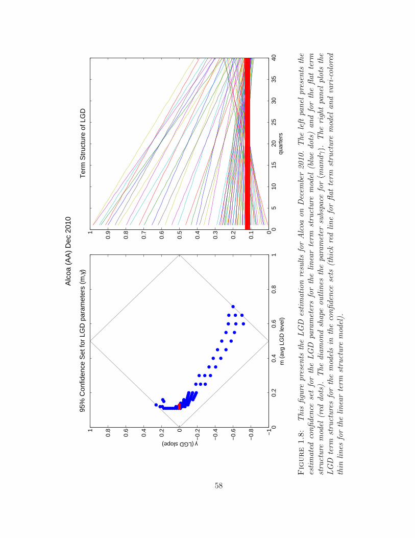
Alc
oa (
AA
) D
ec 2
010
00.
20.
40.
60.
81
−1
−0.
8
−0.
6
−0.
4
−0.
20
0.2
0.4
0.6
0.81
γ (LGD slope)
m (
avg
LGD
leve
l)
95%
Con
fiden
ce S
et fo
r LG
D p
aram
eter
s (m
,γ)
05
1015
2025
3035
400
0.1
0.2
0.3
0.4
0.5
0.6
0.7
0.8
0.91
Ter
m S
truc
ture
of L
GD
quar
ters
Figure1.8
:T
his
figu
repr
esen
tsth
eL
GD
esti
mat
ion
resu
lts
for
Alc
oaon
Dec
embe
r20
10.
The
left
pan
elpr
esen
tsth
ees
tim
ated
con
fide
nce
set
for
the
LG
Dpa
ram
eter
sfo
rth
eli
nea
rte
rmst
ruct
ure
mod
el(b
lue
dots
)an
dfo
rth
efl
atte
rmst
ruct
ure
mod
el(r
eddo
ts).
The
diam
ond
shap
eou
tlin
esth
epa
ram
eter
subs
pace
forpmandγq.
The
righ
tpa
nel
plot
sth
eL
GD
term
stru
ctu
res
for
the
mod
els
inth
eco
nfi
den
cese
ts(t
hick
red
lin
efo
rfl
atte
rmst
ruct
ure
mod
elan
dva
ri-c
olor
edth
inli
nes
for
the
lin
ear
term
stru
ctu
rem
odel
).
58
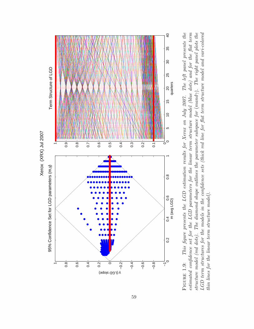
00.
20.
40.
60.
81
−1
−0.
8
−0.
6
−0.
4
−0.
20
0.2
0.4
0.6
0.81
95%
Con
fiden
ce S
et fo
r LG
D p
aram
eter
s (m
,γ)
m (
avg
LGD
)
γ (LGD slope)
Xer
ox (
XR
X)
Jul 2
007
05
1015
2025
3035
400
0.1
0.2
0.3
0.4
0.5
0.6
0.7
0.8
0.91
Ter
m S
truc
ture
of L
GD
quar
ters
Figure
1.9
:T
his
figu
repr
esen
tsth
eL
GD
esti
mat
ion
resu
lts
for
Xer
oxon
Ju
ly20
07.
The
left
pan
elpr
esen
tsth
ees
tim
ated
con
fide
nce
set
for
the
LG
Dpa
ram
eter
sfo
rth
eli
nea
rte
rmst
ruct
ure
mod
el(b
lue
dots
)an
dfo
rth
efl
atte
rmst
ruct
ure
mod
el(r
eddo
ts).
The
diam
ond
shap
eou
tlin
esth
epa
ram
eter
subs
pace
forpmandγq.
The
righ
tpa
nel
plot
sth
eL
GD
term
stru
ctu
res
for
the
mod
els
inth
eco
nfi
den
cese
ts(t
hick
red
lin
efo
rfl
atte
rmst
ruct
ure
mod
elan
dva
ri-c
olor
edth
inli
nes
for
the
lin
ear
term
stru
ctu
rem
odel
).
59

2
Does Anything Beat 5-Minute RV? A Comparisonof Realized Measures Across Multiple Asset Classes
(Joint with Andrew Patton and Kevin Sheppard)
2.1 Introduction
In the past fifteen years, many new estimators of asset return volatility constructed
using high frequency price data have been developed (see Andersen et al. (2006),
Barndorff-Nielsen and Shephard (2007), Meddahi et al. (2011) and Aıt-Sahalia and
Jacod (2014), inter alia, for recent surveys and collections of articles). These esti-
mators generally aim to estimate the quadratic variation or the integrated variance
of a price process over some interval of time, such as one day or week. We refer
to estimators of this type collectively as “realized measures”. This area of research
has provided practitioners with an abundance of alternatives, inducing demand for
some guidance on which estimators to use in empirical applications. In addition to
selecting a particular estimator, these nonparametric measures often require addi-
tional choices for their implementation. For example, the practitioner must choose
60

the sampling frequency to use and whether to sample prices in calendar time (every x
seconds) or tick-time (every x trades). When both transaction and quotation prices
are available, the choice of which price to use also arises. Finally, some realized mea-
sures further require choices about tuning parameters such as a kernel bandwidth or
“block size.”
The aim of this paper is to provide guidance on the choice of realized measure
to use in applications. We do so by studying the performance of a large number
of realized measures across a broad range of financial assets. In total we consider
over 400 realized measures, across eight distinct classes of estimators, and we apply
these to 11 years of daily data on 31 individual financial assets covering five asset
classes. We compare the realized measures in terms of their estimation accuracy
for the latent true quadratic variation, and in terms of their forecast accuracy when
combined with a simple and well-known forecasting model. We employ model-free
data-based comparison methods that make minimal assumptions on properties of
the efficient price process or on the market microstructure noise that contaminates
the efficient prices.
To our knowledge, no existing papers have used formal tests to compare the
estimation accuracy of a large number of realized measures using real financial data.
The fact that the target variable (quadratic variation) is latent, even ex-post, creates
an obstacle to applying standard techniques. Previous research on the selection of
estimators of quadratic variation has often focused on recommending a sampling
frequency based on the underlying theory using plug-in type estimators of nuisance
parameters. For some estimators, a formula for the optimal sampling frequency
under a set of assumptions is derived and can be computed using estimates of higher
order moments, see Bandi and Russell (2008) among others. However, these formulas
are usually heavily dependent on assumptions about the microstructure noise and
61

efficient price process, such as independence of the noise from the price and a lack
of serial correlation in the noise. Gatheral and Oomen (2010) use simulated data
from an agents-based model to evaluate a variety of realized measures, and include
recommendations on data sampling and implementing the estimators they study.
Many papers that introduce novel realized measures provide evidence that details
the new estimator’s advantages over previous estimators. This evidence can be in the
form of theoretical properties of estimators such as consistency, asymptotic efficiency,
and rate of convergence, or results from Monte Carlo simulations using common
stochastic volatility models. These comparisons inevitably require making specific
assumptions on important properties of the price process. Empirical applications
are also common, although typically only a small number of assets from a single
asset class are used, and it is rare that any formal comparison testing is carried out.
Moreover, most papers proposing new estimators consider (perhaps reasonably) only
a relatively small range of alternative estimators.
Our objective is to compare a large number of available realized measures in
a unified, data-based framework. We use the data-based ranking method of Patton
(2011a), which makes no assumptions about the properties of the market microstruc-
ture noise, aside from standard moment and mixing conditions. The main contri-
bution of this paper is an empirical study of the relative performance of estimators
of daily quadratic variation from 8 broad classes of realized measures using data
from 31 financial assets spanning different classes. We obtain tick-by-tick transac-
tion and quotation prices from January 2000 to December 2010, and additionally
sample prices in calendar-time and tick-time, using sampling frequencies varying
from 1 second to 15 minutes. We use the “model confidence set”of Hansen et al.
(2011) to construct sets of realized measures that contain the best measure with
a given level of confidence. We are also interested whether a simple RV estimator
62

with a reasonable choice of sampling frequency, namely 5-minute RV, can stand in
as a “good enough” estimator for QV, for the assets we consider. This is similar
to the comparison of more sophisticated volatility models with a simple benchmark
model presented in Hansen and Lunde (2005). We use the step-wise multiple testing
method of Romano and Wolf (2005), which allows us to determine whether any of
the 400+ competing realized measures is significantly more accurate than a simple
realized variance measure based on 5-minute returns. We also conduct an out-of-
sample forecasting experiment to study the accuracy of volatility forecasts based on
these individual realized measures, when used in the “heterogeneous autoregressive”
(HAR) forecasting model of Corsi (2009), for forecast horizons ranging from 1 to 50
trading days.
Finally, we undertake a panel investigation of the market microstructure and
market condition variables that explain the differences in the accuracy of the real-
ized measures considered in this paper. While 5-minute RV is beaten on average
by (well-chosen) more sophisticated alternatives, the differences are smaller when
microstructure noise, somehow measured, is higher, or when volatility is higher. In-
terestingly, we also find that more sophisticated realized measures generally perform
significantly worse in non-US markets than in US markets, the latter having been
the focus of much of this literature. This is potentially indicative of different market
microstructure effects in non-US markets, which may be better handled with new
approaches.
The remainder of this paper is organized as follows. Section 2 provides a brief
description of the classes of realized measures. Section 3 describes ranking method-
ology and tests used to compare the realized measures. Section 4 describes the high
frequency data and the set of realized measures we construct. Our main analysis is
presented in Section 5, and Section 6 concludes.
63

2.2 Measures of asset price variability
To fix ideas and notation, consider a general jump-diffusion model for the log-price
p of an asset:
dp ptq µ ptq dt σ ptq dW ptq κ ptq dN ptq (2.1)
where µ is the instantaneous drift, σ is the (stochastic) volatility, W is a standard
Brownian motion, κ is the jump size, and N is a counting measure for the jumps.
In the absence of jumps the third term on the right-hand side above is zero. The
quadratic variation of the log-price process over period t 1 is defined
QVt1 plimnÑ8
n
j1
r2tjn, (2.2)
rtjn ptjn ptpj1qn
where the price series on day t 1 is assumed to be observed n times tpt1n, ...,
pt11n, pt1u. See Andersen et al. (2006), Barndorff-Nielsen and Shephard (2007)
and Aıt-Sahalia and Jacod (2014) for surveys of volatility estimation and forecasting
using high frequency data. The objective of this paper is to compare the variety of
estimators of QV that have been proposed in the literature to date. We do so with
emphasis on comparisons with the simple realized variance estimator, which is the
empirical analog of QV:
RVt1 n
j1
r2tjn. (2.3)
2.2.1 Sampling frequency, sampling scheme, and sub-sampling
We consider a variety of classes of estimators of asset price variability. All realized
measures require a choice of sampling frequency (e.g., 1-second or 5-minute sam-
64

pling), sampling scheme (calendar time or tick time), whether to use transaction
prices or mid-quotes, when both are available. Thus even for a very simple estimator
such as realized variance, there are a number of choices to be made. To examine the
sensitivity of realized measures to these choices, we implement each measure using
calendar-time sampling of 1 second, 5 seconds, 1 minute, 5 minutes and 15 minutes.
We also consider tick-time sampling using samples that yield average durations that
match the values for calendar-time sampling, as well as a “tick-by-tick” estimator
that simply uses every available observation. Subsampling,1 introduced by Zhang
et al. (2005), is a simple way to improve efficiency of some sparse-sampled estima-
tors. We consider subsampled versions of all estimators (except estimators using
tick-by-tick data, which cannot be subsampled).2 The sub-sampled version of RV
(which turns out to perform very well in our analysis) was first studied as the “second
best” estimator in Zhang et al. (2005).
In total we have 5 calendar-time implementations, 6 tick-time implementations,
and 5+6–1=10 corresponding subsampled implementations, yielding 21 realized mea-
sures for a given price series. Estimating these on both transaction and quote prices
yields a total of 42 versions of each realized measure. Of course, some of these com-
binations are expected to perform poorly empirically (given the extant literature on
microstructure biases and the design of some of the estimators described below), and
by including them in our analysis we thus have an “insanity check” on whether our
tests can identify these poor estimators.
1 Subsampling involves using multiple “grids” of prices sampled at a given frequency to obtain acollection of realized measures, which are then averaged to yield the “subsampled” version of theestimator. For example, 5-minute RV can be computed using prices sampled at 9:30, 9:35, etc. andcan also be computed using prices sampled at 9:31, 9:36, etc.
2 In general, we implement subsampling using a maximum of 10 partitions.
65

2.2.2 Classes of realized measures
The first class of estimators is standard realized variance (RV), which is the sum of
squared intra-daily returns. This simple estimator is the sample analog of quadratic
variation, and in the absence of noisy data, it is the nonparametric maximum likeli-
hood estimator, and so is efficient, see Andersen et al. (2001b) and Barndorff-Nielsen
(2002). However, market microstructure noise induces serial auto-correlation in the
observed returns, which biases the realized variance estimate at high sampling fre-
quencies (see Hansen and Lunde (2006b) for a detailed analysis of the effects of mi-
crostructure noise). When RV is implemented in practice, the price process is often
sampled sparsely to strike a balance between increased accuracy from using higher
frequency data and the adverse effects of microstructure noise. Popular choices in-
clude 1-minute, 5-minute (as in the title of this paper), or 30-minute sampling.
We next draw on the work of Bandi and Russell (2008), who propose a method
for optimally choosing the sampling frequency to use with a standard RV estimator.
This sampling frequency is calculated using estimates of integrated quarticity3 and
variance of the microstructure noise. These authors also propose a bias-corrected
estimator that removes the estimated impact of market microstructure noise. Since
the key characteristic of the Bandi-Russell estimator is the estimated optimal sam-
pling frequency, we do not vary the sampling frequency when implementing it. This
reduces the number of versions of this estimator from 42 to 8.4
The third class of realized measures we consider is the first-order autocorrelation-
adjusted RV estimator (RVac1) used by French et al. (1987) and Zhou (1996), and
3 Estimates of daily integrated quarticity are estimated using 39 intra-day prices sampled uniformlyin tick-time.
4 Note that the Bandi-Russell RV measure is not consistent for QV in the presence of jumps.(This is also the case for realized range and MLRV, described below.) We include these estimatorsin our comparison as these are widely-used and cited realized measures, and we leave it to the datato shed light on which estimators perform well empirically.
66

studied extensively by Hansen and Lunde (2006b). This estimator was designed to
capture the effect of autocorrelation in high frequency returns induced by market
microstructure noise.
The fourth class of realized measures includes the two-scale realized variance
(TSRV) of Zhang et al. (2005) and the multi-scale realized variance (MSRV) of
Zhang (2006). These estimators compute a subsampled RV on one or more slower
time scales (lower frequencies) and then combine with RV calculated on a faster
time scale (higher frequency) to correct for microstructure noise. Under certain
conditions on the market microstructure noise, these estimators are consistent at
the optimal rate. In our analysis, we set the faster time scale by using one of the
21 sampling frequency/sampling scheme combinations mentioned above, while the
slower time scale(s) are chosen to minimize the asymptotic variance of the estimator
using the methods developed in the original papers. It is worth noting here that
“subsampled RV”, which we have listed in our first class of estimators, corresponds
to the “second-best” form of TSRV in Zhang et al. (2005), in that it exploits the
gains from subsampling but does not attempt to estimate and remove any bias in this
measure. We keep any measure involving two or more time scales in the TSRV/MSRV
class, and any measure based on a single time scale is listed in the RV class.
The fifth class of realized measures is the realized kernel (RK) estimator of
Barndorff-Nielsen et al. (2008). This measure is a generalization of RVac1, ac-
commodating a wider variety of microstructure effects and leading to a consistent
estimator. Barndorff-Nielsen et al. (2008) present realized measures using several
different kernels, and we consider RK with the “flat top” versions of the Bartlett,
cubic, and modified Tukey-Hanning2 kernel, and the “non-flat-top”Parzen kernel.
The Bartlett and cubic RK estimators are asymptotically equivalent to TSRV and
MSRV, respectively, and modified Tukey-Hanning2 was the recommended kernel in
67

Barndorff-Nielsen et al. (2008) in their empirical application to GE stock returns.
The non-flat-top Parzen kernel was studied further in Barndorff-Nielsen et al. (2011)
and results in a QV-estimator that is always positive while allowing for dependence
and endogeneity in the microstructure noise. We implement these realized kernel es-
timators using the 21 sampling frequency/sampling scheme combinations mentioned
above, and estimate the optimal bandwidths for these kernels separately for each
day, using the methods in Barndorff-Nielsen et al. (2011). The realized kernel esti-
mators are not subsampled because Barndorff-Nielsen et al. (2011) report that for
“kinked” kernels such as the Bartlett kernel, the effects of subsampling are neutral,
while for the other three “smooth” kernels, subsampling is detrimental. (The RVac1
measure corresponds to the use of a “truncated” kernel, and subsampling improves
performance, so we include the subsampled versions of RVac1 in the study.)
The sixth class of estimators are pre-averaged realized variances (RVpa) estima-
tors first introduced by Podolskij and Vetter (2009a) and further studied in Jacod
et al. (2009). Pre-averaging applies a kernel-like weighting function to observed re-
turns to construct pre-averaged returns. The most common weighting function has
a Bartlett kernel-like tent shape and so it is identical to first locally averaging prices
and then constructing returns as the difference between two adjacent pre-averaged
prices. Pre-averaged realized variance and realized kernels are closely related, and
in general only differ in the treatment of edge effects – the handling of the first and
last few observations. Given a particular sampling scheme, RVpa is implemented
using all (overlapping) pre-averaged returns. Following the empirical work of Chris-
tensen et al. (2014) and Hautsch and Podolskij (2013), we use a kernel bandwidth
K rθ?ns, where θ 1 and n is the number of sampled intraday returns.
The seventh class of estimators is the “realized range-based variance” (RRV) of
Christensen and Podolskij (2007) and Martens and Van Dijk (2007). Early research
68

by Parkinson (1980), Andersen and Bollerslev (1998) and Alizadeh et al. (2002) show
that the properly scaled, daily high-low range of log prices is an unbiased estimator
of daily volatility when constant, and is more efficient than squared daily open-to-
close returns. Correspondingly, Christensen and Podolskij (2007) and Martens and
Van Dijk (2007) apply the same arguments to intraday data, and improve on the
RV estimator by replacing each intraday squared return with the high-low range
from a block of intra-day returns. To implement RRV, we use the sampling schemes
described above, and then use block size of 5, following Patton and Sheppard (2009b),
and block size of 10, which is close to the average block size used in Christensen and
Podolskij’s application to General Motors stock returns.
Finally, we include the maximum likelihood Realized Variance (MLRV) of Aıt-
Sahalia et al. (2005), which assumes that the observed price process is composed of
the efficient price plus i.i.d. noise such that the observed return process follows an
MA(1) process with parameters that can be estimated using Gaussian MLE. This
estimator is shown to be robust to misspecification of the marginal distribution of the
microstructure noise by Aıt-Sahalia et al. (2005), but is sensitive to the independence
assumption of noise, as demonstrated in Gatheral and Oomen (2010).
The total number of realized measures we compute for a single price series is
210, so an asset with both transactions and quote data has a set of 420 realized
measures.5,6
5 Specifically, for each of RV, RVpa, TSRV, MSRV, MLRV, RVac1, RRV (with two choices of blocksize) and RK (with 4 different kernels), 11 not-subsampled estimators, which span different samplingfrequencies and sampling schemes, are implemented on each of the transactions and midquotes priceseries. In addition, we estimate 2 bias-corrected Bandi-Russell realized measures and 2 not-bias-corrected BR measures (calendar-time and tick-time sampling) per price series. These estimatorsaccount for 12 11 2 p2 2q 2 272 of the total set. RV, TSRV, MSRV, MLRV, RVac1 andRRV (m=5 and 10) also have 10 subsampled estimators per price series, and there are 4 subsampledBR estimators per price series, which adds 7102 + 42 = 148 subsampled estimators to the set.In total, this makes 272+148=420 estimators.
6 Research on estimating volatility using high-frequency data has continued since this projectbegan, and some new estimators have recently been proposed that are not included in our analysis,
69

2.2.3 Additional realized measures
Our main empirical analysis focuses on realized measures that estimate the quadratic
variation of an asset price process. From a forecasting perspective, work by Andersen
et al. (2007) and others has shown that there may be gains to decomposing QV into
the component due to continuous variation (integrated variance, or IV) and the
component due to jumps (denoted JV):
QVt1 plimnÑ8
n
j1
r2tjn
» t1
t
σ2 psq dsloooooomoooooonIVt1
¸
t s¤t1
κ2 psqloooooomoooooonJVt1
(2.4)
Thus for our forecasting application in Section 2.5.6, we also consider four classes
of realized measures that are “jump robust”, i.e., they estimate IV not QV. The
first of these is the bi-power variation (BPV) of Barndorff-Nielsen and Shephard
(2006), which is a scaled sum of products of adjacent absolute returns. We also
estimate a pre-averaged version of Bipower Variation, motivated by Podolskij and
Vetter (2009b) and Christensen et al. (2014).
The second class of jump-robust realized measures is the quantile-based realized
variance (QRV) of Christensen et al. (2010). QRV is based on combinations of locally
extreme quantile observations within blocks of intra-day returns, and requires choice
of block length and quantiles. It is reported to have better finite sample performance
than BPV in the presence of jumps, and additionally is consistent, efficient and
jump-robust even in the presence of microstructure noise. For implementation, we
use the asymmetric version of QRV with rolling overlapping blocks7 and quantiles
e.g., the estimators of Bibinger et al. (2014) and Jacod and Todorov (2014).
7 Christensen et al. (2010) refers to this formulation of the QRV as “subsampled QRV”, as op-posed to “block QRV”, which has adjacent non-overlapping blocks. However, we do not use thisterminology as this type of “subsampling” is different from the subsampling we implement for the
70

approximately equal to 0.85, 0.90 and 0.96, following the authors’ application to
Apple stock returns. The block lengths are chosen to be around 100, with the exact
value depending on the number of filtered daily returns, and the quantile weights
are calculated optimally following the method in Christensen et al. (2010). QRV
is the most time-consuming realized measure to estimate, and thus is not further
subsampled.
The third class of jump-robust realized measures are the “nearest neighbor trunca-
tion” estimators of Andersen et al. (2012), specifically their “MinRV” and “MedRV”
estimators. These are the scaled square of the minimum of two consecutive intra-day
absolute returns or the median of 3 consecutive intra-day absolute returns. These es-
timators are more robust to jumps and microstructure noise than BPV, and MedRV
is designed to handle outliers or incorrectly entered price data.
The final class of jump-robust measures estimators is the truncated or threshold
realized variance (TRV) of Mancini (2001, 2009), which is the sum of squared returns,
but only including returns that are smaller in magnitude than a certain threshold.
Following Corsi et al. (2010), we take the threshold to be be three times a local
(intra-day) volatility estimate.8
In total, across sampling frequencies and subsampling/not subsampling we in-
clude 228 jump-robust realized measures in our forecasting application, in addition
to the 420 estimators described in the previous section.
other estimators.
8 The algorithm to compute local volatility can fail when very high-frequency sampling is appliedto days with low liquidity, and in such cases we consider the TRV to be non-implementable. Theseoccurrences are generally limited to 1-second sampling or, less often, 5-second sampling of illiquidassets such as computed indices or individual equities.
71

2.3 Comparing the accuracy of realized measures
We examine the empirical accuracy of our set of competing measures of asset price
variability using two complementary approaches.
2.3.1 Comparing estimation accuracy
We first compare the accuracy of realized measures in terms of their estimation
error for a given day’s quadratic variation. QV is not observable, even ex post,
and so we cannot directly calculate a metric like mean-squared error and use that
for the comparison. We overcome this by using the data-based ranking method
of Patton (2011a). This approach requires employing a proxy (denoted θ) for the
quadratic variation that is assumed to be unbiased, but may be noisy.9 This means
that we must choose a realized measure that is unlikely to be affected by market
microstructure noise. Using proxies that are more noisy will reduce the ability to
discriminate between estimators, but will not affect consistency of the procedure. We
use the squared open-to-close returns from transaction prices (RVdaily) for our main
analysis, and further consider 15-minute RV, 5-minute RV, 1-minute MSRV and
1-minute RKth2, all computed on transaction prices using tick-time sampling, as
possible alternatives.10 Since estimators based on the same price data are correlated,
it is necessary to use an instrument for the proxy to “break”the dependence between
the estimation error in the realized measure under analysis and the estimation error
in the proxy. As our instrument we use a one-day lead of the proxy.11
9 Numerous estimators of quadratic variation can be shown to be asymptotically unbiased as thesampling interval goes to zero, however this approach requires unbiasedness for a fixed samplinginterval.
10 These four additional proxies were found to be unbiased for the RVdaily measure for the majorityof assets, and in addition, are generally much more precise.
11 As described in Patton (2011a), the use of a lead (or lag) of the proxy formally relies on thedaily quadratic variation following a random walk. Numerous papers, see Bollerslev et al. (1994)
72

The comparison of estimation accuracy also, of course, requires a metric for mea-
suring accuracy. The approach of Patton (2011a) allows for a variety of metrics,
including the MSE and QLIKE loss functions. Simulation results in Patton and
Sheppard (2009a), and empirical results in Hansen and Lunde (2005), Patton and
Sheppard (2009b) and Patton (2011a) all suggest that using QLIKE leads to more
power to reject inferior estimators.12 The QLIKE loss function is defined as:
QLIKE L pθ,Mq θ
M log
θ
M 1 (2.5)
where θ is QV, or a proxy for it, and M is a realized measure. With this in hand, we
obtain a consistent (as T Ñ 8) estimate of the difference in accuracy between any
two realized measures:
1
T
T
t1
∆Lij,tpÝÑ E r∆Lij,ts (2.6)
where ∆Lij,t Lθt,Mit
L
θt,Mjt
and ∆Lij,t L pθt,Mitq L pθt,Mjtq .
Under standard regularity conditions (see Patton (2011a) for example) we can use
a block bootstrap to conduct tests on the estimated differences in accuracy, such as
the pair-wise comparisons of Diebold and Mariano (2002) and Giacomini and White
and Andersen et al. (2006) for example, find that conditional variance is a highly persistent pro-cess, close to being a random walk. Hansen and Lunde (2014) study the quadratic variation ofall 30 constituents of the Dow Jones Industrial Average and reject the null of a unit root for fewof the stocks. Meddahi (2003) shows analytically that certain classes of continuous time stochas-tic volatility processes imply that their daily integrated variance follows an ARMA process, withautoregressive persistence governed by the persistence of the spot variance. Simulation results inPatton (2011a) show that inference based on a random walk approximation has acceptable finite-sample properties for DGPs that are persistent but strictly not random walks, and we confirm inTable A4, in the appendix, that all series studied here are highly persistent. In Section 2.5 we alsopresent results based on an AR(1) approximation rather than a random walk. We also consider theuse of a one-day lag of the proxy, and find the results (reported in the appendix) to be very similarto our base case using a one-day lead.
12 We also present some results based on the MSE loss function. See Section 2.5 and the onlineappendix.
73

(2006), the “reality check” of White (2000) as well as the multiple testing procedure
of Romano and Wolf (2005), and the “model confidence set” of Hansen et al. (2011).
2.3.2 Comparing forecast accuracy
The second approach we consider for comparing realized measures is through a simple
forecasting model. As we describe in Section 2.5.6 below, we construct volatility
forecasts based on the heterogeneous autoregressive (HAR) model of Corsi (2009),
estimated separately for each realized measure. The problem of evaluating volatility
forecasts has been studied extensively, see Hansen and Lunde (2005), Andersen et al.
(2005), Hansen and Lunde (2006a) and Patton (2011b) among several others. The
latter two papers focus on applications where an unbiased volatility proxy is available,
and again under standard regularity conditions we can use block bootstrap methods
to conduct tests such as those of Diebold and Mariano (2002), White (2000), Romano
and Wolf (2005), Giacomini and White (2006), and Hansen et al. (2011).
2.4 Data description
We use high frequency (intra-daily) asset price data for 31 assets spanning five as-
set classes: individual equities (from the U.S. and the U.K.), equity index futures,
computed stock indices, currency futures and interest rate futures. The data are
transactions and quotations prices taken from Thomson Reuter’s Tick History. The
sample period is January 2000 to December 2010, though data availability limits
us to a shorter sub-period for some assets. Short days, defined as days with prices
recorded for less than 60% of the regular market operation hours, are omitted. For
each asset, the number of short days is small compared to the total number of days
– the largest proportion of days omitted is 1.7% for ES (E-mini S&P500 futures).
Across assets, we have an average of 2537 trading days, with the shortest sample
74

being 1759 trade days (around 7 years) and the longest 2782 trade days. All series
were cleaned according to a set of baseline rules similar to those in Barndorff-Nielsen
et al. (2009). Data cleaning details are provided in the appendix.13
Table 1 presents the list of assets, along with their sample periods and some sum-
mary statistics. Computed stock indices are not traded assets and are constructed
using trade prices, and so quotes are unavailable. This table reveals that these assets
span not only a range of asset classes, but also characteristics: average annualized
volatility ranges from under 2%, for interest rate futures, to over 40%, for individual
equities. The average time between price observations ranges from under one sec-
ond, for the E-mini S&P 500 index futures contract, to nearly one minute, for some
individual equities and computed equity indices.14
Given the large number of realized measures and assets, it is not feasible to present
summary statistics for all possible combinations. Table A1 in the appendix describes
the shorthand used to describe the various estimators15, and in Table 2 we present
summary statistics for a selection of realized measures for two assets, Microsoft and
the US dollar/Australian dollar futures contract.16 Tables A3 and A4 in the appendix
contain more detailed summary statistics. Table 2 reveals some familiar features
of realized measures: those based on daily squared returns have similar averages
13 The sensitivity of estimators in different classes to data cleaning methods is an interesting topic,as is developing estimators that are more robust to various data cleaning rules. We do not explorethese issues. We note here that the data provided by Thomson Reuter’s Tick History, especiallythe data on futures, is very clean compared with the more-widely used NYSE TAQ data.
14 Most futures contracts trade nearly 24 hours a day. However, their liquidity is typically con-centrated around a relatively short interval, usually less than half of the day. We measured thepercentage of trades that occurred in five minute block of the day using local time-stamps to avoidissues with daylight saving changes, and selected the largest contiguous block where the percentageof observations in the block was above 20% of 1/288.
15 For example, “RV 1m ct ss” refers to realized variance (RV), computed on 1-minute data (1m)sampled in calendar time (c), using trade prices (t), with subsampling (ss). See Table A1 for details.
16 All realized measures were computed using code based on Kevin Sheppard’s “Oxford Realized”toolbox for Matlab, https://www.kevinsheppard.com/MFEToolbox.
75

to realized measures using high (but not too high) frequency data, but are more
variable, reflecting greater measurement error. For Microsoft, for example, RVdaily
has an average of 3.20 (28.4% annualized) compared with 3.37% for RV5min, but its
standard deviation is more than 25% larger than that of RV5min. We also note that
RV computed using tick-by-tick sampling (i.e., the highest possible sampling) is much
larger on average than the other estimators, more than 3 times larger for Microsoft
and around 50% larger for the USD/AUD exchange rate, consistent with the presence
of market microstructure noise. This distortion vanishes when pre-averaging is used.
In the last four columns of Table 2 we report the first- and second-order sam-
ple autocorrelations of the realized measures, as well as estimates of the first- and
second-order autocorrelation of the underlying quadratic variation using the estima-
tion method in Hansen and Lunde (2014).17 As expected, the latter estimates are
much higher than the former, reflecting the attenuation bias due to the estimation
error in a realized measure. Using the method of Hansen and Lunde (2014), the esti-
mated first-order autocorrelation of QV for Microsoft and the USD/AUD exchange
rate is around 0.95, while the sample autocorrelations for the realized measures them-
selves average around 0.68. Table A4 presents summaries of these autocorrelations
for all 31 assets, and reveals that the estimated first- (second-) order autocorrelation
of the underlying QV is high for all assets. The average estimate across all assets and
realized measures, even including poor estimators, equals 0.95 (0.92). These findings
support our use, in the next section, of the ranking method of Patton (2011a), which
relies on high persistence of QV.
17 Following their empirical application to the 30 DJIA stocks, we use the demeaned 4th through10th lags of the daily QV estimator as instruments.
76

2.5 Empirical results on the accuracy of realized measures
We now present the main analysis of this paper. We firstly discuss simple rankings
of the realized measures, and then move on to more sophisticated tests to formally
compare the various measures. As described in Section 2.3, we measure accuracy
using the QLIKE distance measure, using squared open-to-close returns (RVdaily)
as the volatility proxy, with a one-day lead to break the dependence between esti-
mation error in the realized measure and error in the proxy. In some of the analysis
below we consider using higher frequency RV measures for the proxy (RV15min and
RV5min), as well as some non-RV proxies, namely 1-minute MSRV and 1-minute
Tukey-Hanning2 realized kernel.
2.5.1 Rankings of average accuracy
We firstly present a summary of the rankings of the 420 realized measures applied to
the 31 assets in our sample. These rankings are based on average, unconditional dis-
tance of the measure from the true QV, and in Section 2.5.5 we consider conditional
rankings.
The top panel of Table 3 presents the “top 10” individual realized measures,
according to their average rank across all assets in a given class.18 It is noteworthy
that 5-minute RV does not appear in the top 10 for any of these asset classes. This
is some initial evidence that there are indeed better estimators of QV available, and
we test whether this outperformance is statistically significant in the sections below.
With the caveat that these estimated rankings do not come with any measures
of significance, and that realized measures in the same class are likely highly cor-
18 Table A6 in the appendix presents rank correlation matrices for each asset class, and confirmsthat the rankings of realized measures for individual assets in a given asset class are relativelyconsistent, with average within-asset-class rank correlations ranging from 0.70 to 0.87.
77

related19, we note the following patterns in the results. Realized kernels appear to
do well for individual equities (taking 4 and 5 of the top 10 slots, respectively, for
US and UK equities), realized range does well for interest rate futures (8 out of top
10), and two/multi-scales RV do well for currency futures (6 out of the top 10). For
computed indices, RVac1 and realized kernels comprise the entire top 10. The top 10
realized measures for index futures contain a smattering of measures across almost all
classes. The lower panel of Table 3 presents a summary of the upper panel, sorting
realized measures by class and sampling frequency.
It is perhaps also interesting to note which price series is most often selected. We
observe a mix of trades and quotes for individual equities,20 while we see mid-quotes
dominating the top 10 for interest rate futures and currency futures. For equity
index futures, transaction prices make up the entire top 10. (Our computed indices
are only available with transaction prices, so no comparisons are available for that
asset class.)
2.5.2 Pair-wise comparisons of realized measures
To better understand the characteristics of a “good” realized measure, we present
results on pair-wise comparisons of measures that differ only in one aspect. We
consider four features: the use of transaction prices vs. mid-quotes; the use of
calendar-time vs. tick-time sampling; the use of subsampling; and the use of pre-
averaging. For each class of realized measures and for each sampling frequency, we
compare pairs of estimators that differ in one of these dimensions, and compute a
19 See Table A5 in the appendix for a summary of the correlations between realized measures.
20 In fact, decomposing this group into US equities and UK equities, we see that the top 10realized measures for US equities all use transaction prices, while the top 10 for UK equities all usemid-quotes, perhaps caused by different forms of market microstructure noise on the NYSE (theexchange for 4 of the 5 U.S. stocks) and the LSE.
78
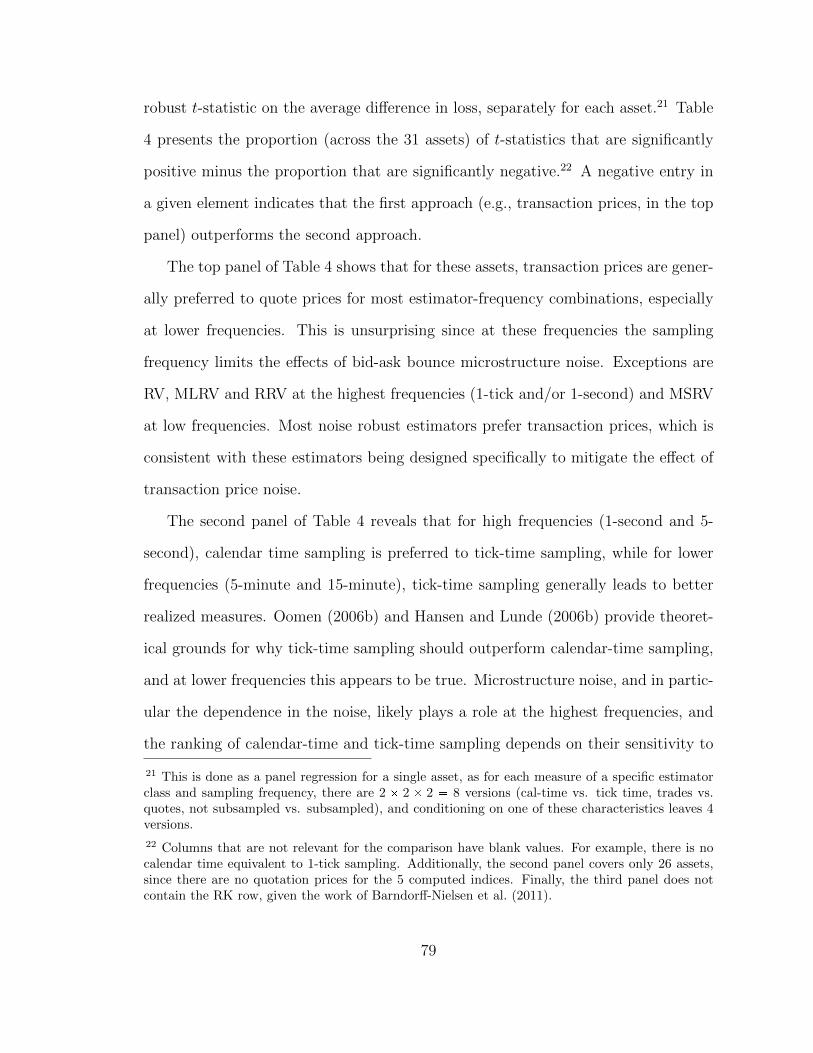
robust t-statistic on the average difference in loss, separately for each asset.21 Table
4 presents the proportion (across the 31 assets) of t-statistics that are significantly
positive minus the proportion that are significantly negative.22 A negative entry in
a given element indicates that the first approach (e.g., transaction prices, in the top
panel) outperforms the second approach.
The top panel of Table 4 shows that for these assets, transaction prices are gener-
ally preferred to quote prices for most estimator-frequency combinations, especially
at lower frequencies. This is unsurprising since at these frequencies the sampling
frequency limits the effects of bid-ask bounce microstructure noise. Exceptions are
RV, MLRV and RRV at the highest frequencies (1-tick and/or 1-second) and MSRV
at low frequencies. Most noise robust estimators prefer transaction prices, which is
consistent with these estimators being designed specifically to mitigate the effect of
transaction price noise.
The second panel of Table 4 reveals that for high frequencies (1-second and 5-
second), calendar time sampling is preferred to tick-time sampling, while for lower
frequencies (5-minute and 15-minute), tick-time sampling generally leads to better
realized measures. Oomen (2006b) and Hansen and Lunde (2006b) provide theoret-
ical grounds for why tick-time sampling should outperform calendar-time sampling,
and at lower frequencies this appears to be true. Microstructure noise, and in partic-
ular the dependence in the noise, likely plays a role at the highest frequencies, and
the ranking of calendar-time and tick-time sampling depends on their sensitivity to
21 This is done as a panel regression for a single asset, as for each measure of a specific estimatorclass and sampling frequency, there are 2 2 2 8 versions (cal-time vs. tick time, trades vs.quotes, not subsampled vs. subsampled), and conditioning on one of these characteristics leaves 4versions.
22 Columns that are not relevant for the comparison have blank values. For example, there is nocalendar time equivalent to 1-tick sampling. Additionally, the second panel covers only 26 assets,since there are no quotation prices for the 5 computed indices. Finally, the third panel does notcontain the RK row, given the work of Barndorff-Nielsen et al. (2011).
79
this noise. RVpa and RK appear to be insensitive to the sampling scheme at the
highest frequencies.
The third panel of Table 4 compares realized measures with and without sub-
sampling. Theoretical work by Zhang et al. (2005) and Zhang (2006) suggests that
subsampling is a simple way to improve the efficiency of a realized measure. Our
empirical results generally confirm that subsampling is helpful, at least when using
lower frequency (5-minute and 15-minute) data. For higher frequencies (1-second to
1-minute), subsampling has either no effect or a negative effect on accuracy. Inter-
estingly, we note that for realized range (RRV), subsampling reduces accuracy across
all sampling frequencies.
Finally, the bottom panel presents clear advice on pre-averaging: it is beneficial
at the highest sampling frequencies (5 seconds or less) and harmful at frequencies
lower than one minute. This is consistent with the theoretical underpinnings of pre-
averaging, see Podolskij and Vetter (2009a) and Jacod et al. (2009), both of which
suggest applying pre-averaging to data sampled at the highest frequency.
2.5.3 Does anything beat 5-minute RV?
Realized variance, computed with a reasonable choice of sampling frequency, is often
taken as a benchmark or rule-of-thumb estimator for volatility, see Andersen et al.
(2001a) and Barndorff-Nielsen (2002) for example. This measure has been used
as far back as French et al. (1987), is simple to compute, and when implemented
on a relatively low sampling frequency (such as five minutes) requires much less
data and cleaning.23 Thus it is of great interest to know whether it is significantly
23 Of course, a sampling frequency of five minutes is only “relatively low” for liquid assets; forsome assets, such as corporate bonds, a five-minute sampling frequency would be quite high. Five-minute sampling has emerged as a rough benchmark in the extant literature since the vast majorityof empirical studies look at very liquid assets like exchange rates and U.S. equities. Given that allof our 31 assets are relatively liquid, we adopt five-minute RV as our benchmark estimator.
80

outperformed by one of the many more sophisticated realized measures proposed in
the literature.
We use the stepwise multiple testing method of Romano and Wolf (2005) to
address this question. The Romano-Wolf method tests the unconditional accuracy
of a set of estimators relative to that of a benchmark realized measure, which we
take to be RV computed using 5-minute calendar-time sampling on transaction prices
(which we denote RV5min). This procedure is an extension of the “reality check” of
White (2000), allowing us to determine not only whether the benchmark measure is
rejected, but to identify the competing measures that led to the rejection. Formally,
the Romano-Wolf stepwise method examines the set of null hypotheses:
Hpsq0 : E rL pθt,Mt,0qs E rL pθt,Mt,sqs , for s 1, 2, ..., S (2.7)
and looks for realized measures, Mt,s, such that eitherE rL pθt,Mt,0qs ¡ E rL pθt,Mt,sqsor E rL pθt,Mt,0qs E rL pθt,Mt,sqs . The Romano-Wolf procedure controls the “family-
wise error rate”, which is the probability of making one or more false rejections among
the set of hypotheses. We run the Romano-Wolf test in both directions, first to iden-
tify the set of realized measures that are significantly worse than RV5min, and then
to identify the set of realized measures that are significantly better than RV5min.
We implement the Romano-Wolf procedure using the Politis and Romano (1994)
stationary bootstrap with 1000 bootstrap replications and an average block size of
10 days.24 A summary of results is presented in Table 5, and detailed results can be
24 The ideal choice of block size length is driven by the persistence in the variable we are interestedin testing, which in our case is the loss difference, ∆Lpθt,Mt,0,Mt,sq. The QLIKE loss, which isbased on the realized measure and a proxy, is substantially less persistent than the realized measure,and by taking the difference between two measures and a proxy we further reduce the persistence.To confirm this, we compute the optimal block length, using the method of Politis and White(2004), for all pairs of measures and all assets. The mean optimal block length for loss differencesis 4, and the median is 2. In contrast, the mean optimal block length for the measures themselvesis 97, and the median is 103. A block length of 10 for the loss differences is thus a reasonably
81
found in the online appendix.
The striking feature of Table 5 is the preponderance of estimators that are signif-
icantly beaten by RV5min, and the almost complete lack of estimators that signifi-
cantly beat RV5min. Concerns about potential low power of this inference method
are partially addressed by the ability of this method to reject so many estimators as
significantly worse than RV5min: using RVdaily as the proxy we reject an average
of 193 estimators (out of 420) as significantly worse than RV5min, which represents
almost half of the set of competing measures.25
We also present results using the other four proxies. These proxies are more pre-
cise, although they are potentially more susceptible to market microstructure noise.
(Proxies that have an unconditional mean that is significantly different from that of
RVdaily, an indication of bias, have results in grey rather than black text in Table
5.) Results from the more precise proxies are very similar: we can reject over half
of the competing estimators as being significantly worse than RV5min, but we find
just one asset out of 31 with any measures that significantly outperform RV5min.26
It is worth noting here that Table 5 reveals that the use of a particular realized
measure as a proxy does not lead to an apparent improvement in the performance of
conservative choice.
25 Note that the Romano-Wolf test controls the family-wise error (FWE) rate, defined as theprobability of rejecting a single true null hypothesis across all 420 nulls, and so for each use of theRomano-Wolf test we would expect to falsely reject only 0.05 of a measure. Of course, we run thistest on 31 different assets, and so across all assets we expect one or two of the testing proceduresto result in false rejections.
26 We also implemented the Romano-Wolf procedure swapping the “reality check” step with astep based on the test of Hansen (2005). This latter test is designed to be less sensitive to pooralternatives with large variances (a potential concern in our application) and so should have betterpower. We found no change in the number of rejections. In a more forceful attempt to examinethe sensitivity to poor alternatives: we identified, ex ante, 72 estimators that the existing literaturewould suggest are likely to have poor performance (for example, realized kernels on 15-minutereturns). We removed this group of estimators from the competing set, and conducted the Romano-Wolf procedure on the remainder of the competing set. We found virtually no change in results ofthe tests – in fact, counting across the two Romano-Wolf tests for each of 31 assets, there was onlyone instance where an estimator was found to have different outcome from the original test.
82

measures from the same class. Specifically, using a RV as the proxy does not “favor”
RV measures, and using RK or TSRV does not favor RK or TSRV measures. The
use of a one-day lead of the proxy solves this potential problem.27
The asset for which we find that RV5min is significantly beaten, the 10-year
US Treasury note futures contract (TY), is among the most frequently traded in our
sample. (It is noteworthy, however, that there are five other assets that are even more
frequently traded, see Table 1, but for which we find no realized measure significantly
better than RV5min.) For the 10-year Treasury note, the realized measures that
outperform RV5min include MSRV, RK and RRV all estimated using 1-second or
5-second sampling (in calendar-time or business-time, with or without subsampling),
and 1-minute RV and 1-minute RVac1; a collection of measures that one might expect
to do well for a very liquid asset.
It is also noteworthy, that, combining the set of estimators that are significantly
worse than RV5min (around one half of all estimators) with those that are signifi-
cantly better (approximately zero), leaves, obviously, around one half of the set of
420 estimators that are not significantly different than RV5min in terms of average
accuracy.
To better understand the results of the Romano-Wolf tests applied to this large
collection of assets and realized measures, Table 6 presents the proportion (across
27 In Table A8 of the web appendix we present some variations of the methods used to obtainthe results in Table 5. First, we change the loss function from QLIKE to MSE. Simulation resultsin Patton and Sheppard (2009a), and empirical results in Hansen and Lunde (2005), Patton andSheppard (2009b) and Patton (2011a) suggest that tests based on MSE have lower power thanunder QLIKE, and our results are consistent with this: under MSE we continue to find no caseswhere RV5min is significantly beaten by an alternative, and a reduction in the number of caseswhere RV5min is identified as significantly better than an alternative. Second we consider this testbased on a mean-reverting AR(1) approximation for QV rather than the maintained random walkapproximation. Consistent with the simulation results in Patton (2011a) and the results underMSE, we find similar results to our base case but with lower power. Finally we consider the useof a one-day lag, or an average of the one-day lag and one-day lead, as the proxy rather than theone-day lead. The results are mostly unchanged, indicating that either of these instruments for theday t proxy are also suitable.
83

assets) of estimators that are significantly worse than RV5min by class of estimator
and sampling frequency.28 Darker shaded regions represent “better” estimators, in
the sense that they are rejected less often. Across the five asset classes and the
entire set of assets, we observe a darker region running from the top right to the
bottom left. This indicates that the simpler estimators in the top rows (RV and
variants) do better, on average, when implemented on lower frequency data, such as
1-minute and 5-minute data, while the more sophisticated estimators (RK, MSRV,
TSRV and RRV) do relatively better when implemented on higher frequency data,
such as 1-second and 5-second data.
2.5.4 Estimating the set of best realized measures
The tests in the previous section compare a set of competing realized measures
with a given benchmark measure. The RV5min measure is a reasonable, widely-
used, benchmark estimator, but one might also be interested in determining whether
maintaining that estimator as the “null” gives it undue preferential treatment. To
address this question, we undertake an analysis based on the “model confidence
set” (MCS) of Hansen et al. (2011). Given a set of competing realized measures,
this approach identifies a subset that contains the unknown best estimator with
some specified level of confidence, with the other measures in the MCS being not
significantly different from the true best realized measure. As above, we use the
QLIKE distance and a one-day lead of RVdaily as the proxy for QV, and Politis and
Romano’s (1994) stationary bootstrap with 1000 bootstrap replications and average
block-size equal to 10.29
28 In this table we aggregate across calendar-time and tick-time, trade prices and quote prices, tofocus on the class of realized measure and sampling frequency dimensions.
29 Similar to above, we also consider 15-minute RV, 5-minute RV, 1-minute MSRV, and 1-minuteRKth2 (calendar-time, trades prices) as proxies for QV. Again, we find that using one of these moreaccurate proxies leads to greater power in the test, i.e. smaller model confidence sets. However,
84

The number of realized measures in the model confidence sets varies across indi-
vidual assets, from 2 to 148 (corresponding to a range of 1% to 36% of all measures),
with the average size being 39 estimators, representing just under 10% of our set
of 420 realized measures. Index futures and interest rate futures have the smallest
model confidence sets, containing around 5% of all realized measures, while individ-
ual equities have the largest sets, containing around 17% of all measures. Table A7
in the appendix contains further information on the MCS size for each asset.
In Table 7, we summarize these results by reporting the proportion of estimators
from a given class and given frequency that are included in model confidence sets,
aggregating results across assets. Darker shaded elements represent the “better” re-
alized measures. Table 7 reveals a number of interesting features. Focusing on the
results for all 31 assets, presented in the upper-left panel, we see that the “best” re-
alized measure, in terms of number of appearances in a MCS, is not 5-minute RV but
1-minute subsampled RV. Realized kernels sampled at the one-second frequency also
do very well, as do the preaveraged realized variance estimators. The performance
of these noise robust measures is particularly strong for individual equities, possibly
reflecting this asset class’ position as the focus of most existing empirical work.
Looking across asset classes, we see a similar pattern to that in Table 6: a dark
region of good estimators includes RV and variants based on lower frequency data (5
seconds to 5 minutes) and more sophisticated estimators (RK, MSRV/TSRV, MLRV
and RRV) based on higher frequency data (1 second and 5 seconds). We also observe
that for more liquid asset classes, such as currency futures, interest rate futures, and
index futures, realized measures appear in a MCS more often if based on higher
frequency data. In contrast, for individual equities and for computed equity indices,
the results show similar patterns to those using RVdaily as the proxy, and importantly, we find thatusing a proxy of a certain class (RV, TSRV, RK) does not bias the results of the test in favor ofestimators of the same class. Detailed results can be found in the online appendix.
85

the preferred sampling frequencies are generally lower.
We can also use the estimated model confidence sets to shed light on the particu-
larly poorly performing realized measures. Across all 31 assets, we see that realized
measures based on 15-minute data almost never appear in a MCS. Similarly, we
observe that the more sophisticated realized measures, TSRV/MSRV, MLRV, RK
and RRV are almost never in a MCS when sampling every 5- or 15-minutes, which
appears to be too low for these estimators. In addition, for the highly liquid futures
contracts, even a sampling frequency of 1-minute is not high enough to use with
these sophisticated realized measures. This is consistent with the implementations
of these estimators in the papers that introduced them to the literature, and so is
not surprising.
Overall, the results from the previous section revealed that it was very rare to find
a realized measure that significantly outperformed 5-minute RV. The analysis in this
section, which avoids the need to specify a “benchmark” realized measure, reveals
evidence that some measures are indeed more accurate than 5-minute RV. We find
that 1-minute RV and RVac1, 1-second and 5-second Realized Kernels and Multi-
scale RV, and 5-second and 1-minute Realized Range estimators appear more often
in the MCS than 5-minute RV. Subsampled RV at moderate frequencies (1-minute
or 5-minute) also outperforms regular 5-minute RV.
2.5.5 Explaining performance differences
We now seek to shed light on the factors that explain the differences in the accuracy
of the realized measures considered in this paper. The results in the previous sections
are related to average accuracy over the entire sample period, and in this section we
study relative conditional accuracy using a panel version of the approach of Giaco-
mini and White (2006). This approach enables us to examine whether the relative
86

performance of two realized measures varies with some set of conditioning variables.
We use a panel specification to exploit both the time series and the cross-sectional
information in our data, and we consider a variety of conditioning variables to try
to explain when one measure outperforms another. All of the specifications that we
consider are of the form:
Lpθit,M i0,tqLpθit,M i
j,tq β1jXit1γ1jZiεij,t, for t 1, 2, ...T ; i 1, 2, ..., N (2.8)
where the first realized measure, M i0,t, is taken to be RV5min, and the competing
measure, M ij,t, is one of the better-performing realized measures identified in the
previous section, namely, 5-second MSRV, 1-minute RVac1, 5-second RKth2 and 1-
second MLRV.30 We also include 1-minute RV and RVdaily to study the accuracy
gains from using higher-frequency price data. All of these estimators are computed on
transaction prices with calendar-time sampling. The panel is unbalanced as the assets
do not all trade on the same days, and the maximum dimensions of the panel are T 2860 and N 31. We estimate this model using an unbalanced panel framework and
Driscoll and Kraay (1998) standard errors, which are robust to heteroskedasticity,
serial correlation, and cross-sectional dependence.31
Our conditioning variables include a variety of variablesXit1
that might be
thought to influence the accuracy of realized measures. Numerous measures of mar-
ket liquidity exist in the literature (see Hautsch and Podolskij (2013); Aıt-Sahalia and
30 The fact that we examine realized measures identified as “good” in previous analysis of coursebiases the interpretation of any subsequent tests of unconditional accuracy. In this section we focuson whether the relative performance of these measures varies significantly with some conditioningvariables pX,Zq , and the problem of pre-test bias does not arise here.
31 Panel regressions were estimated using the Stata program “xtscc” (Hoechle (2007)) downloadedfrom http://ideas.repec.org/c/boc/bocode/s456787.html. These standard errors are essentially a“HAC of cross-sectional averages”, and based on the length of the data, the program selects 8 lagsto use for the Newey-West kernel. We also used an alternate version of Driscoll-Kraay standarderrors developed in Vogelsang (2012), which uses fixed-b asymptotic theory, but we found that thedifferences in the standard errors were extremely small in this application.
87

Yu (2009), for examples). We use three measures (see Bandi and Russell (2006) and
Diebold and Strasser (2013), for example) that can be computed each day using our
intraday price and volume data: average time between trades (avgdur); total trade
volume in units of local currency (volm); and average bid-ask spreads (BAsprd). All
three of these variables exhibit a strong trend over our sample period, and so we de-
trend each series using a 60-day moving average.32 Next we look at measures of noise
and jumps in the asset price series. For each day we measure the autocorrelation
in 5-second returns (ac1 5s). The autocorrelations of sampled intraday returns have
been studied in the context of measuring QV (Hansen and Lunde (2006b); Hautsch
and Podolskij (2013)) because they embed information about the properties of mi-
crostructure noise, which may influence the performance of realized measures. We
also include an estimate of relative size of the noise: the per-trade ratio of the noise
variance to the total variance (noiseratio), introduced in Oomen (2006a) and used
by Hautsch and Podolskij (2013),33 and the proportion of QV attributable to jumps
(jumpprop), measured as max pRVt BPVt, 0q RVt (both measures use 5-minute
tick-time sampled trades prices), to see if the magnitude of noise or jump activity
has an effect on realized measure performance. Finally, we include a measure of
volatility (logQV), and for this we use subsampled RV5min. Tables A9 and A10
in the web appendix present some summary statistics on these conditioning vari-
ables, including the full-sample averages by which the variables are de-meaned, and
32 Specifically, we set Xt XtXt60,t1 where Xt60,t1 is the average value of the variableover the past 60 days. We also examined using 120- and 250-day averages and the results werequalitatively similar.
33 We compute noiseratio as in Hautsch and Podolskij (2013): noiseratiot αtpQV tntq, wherethe numerator is the first-order autocorrelation of the tick-by-tick returns, and the denominator is1-tick MLRV scaled by the number of observations on that day.
88

information on their cross-correlations.34,35
Given the panel nature of this analysis, we are also able to include variables pZiqto capture some of the cross-sectional variation in our data. We first include dummy
variables for each asset class (equities, bond futures, FX futures, index futures, and
computed indices), which capture some of the time-invariant features of the markets
on which these assets trade.36 We also include geographic dummy variables (US, UK,
Europe and Asia, with the US dummy dropped to avoid perfect multicollinearity)
to see whether there are differences across countries in the relative performance of
these realized measures.37
Table 8 presents the results of these panel regressions, with each column of this
table representing a separate estimation to compare RV5min with the competing
measure listed in the top row. We present the t-statistics above and the parameter
estimates in parentheses below. We focus on the t-statistics since, like Diebold-
Mariano-type tests, the average loss differential, or in this case, the conditional loss
34 We winsorize all conditioning variables at the 0.5% and 99.5% levels to reduce the impact ofextreme observations, and we de-mean all conditioning variables so that the coefficients on thedummy variables can be interpreted as the average loss difference when all conditioning variablesare at their full-sample average values. Finally, we normalize the loss differences by their full-sample standard deviations so that the parameter estimates in Table 8 below are comparable acrosscolumns.
35 The two strongest correlations are between avgdur and volm at -0.66, and ac1 5s and noiseratioat -0.33. logQV is also mildly correlated to all of the conditioning variables except jumpprop, withcorrelation magnitudes ranging from 0.22 to 0.32. The remaining cross-correlations are fairly small.
36 We do not have measures of volume and bid-ask spreads for our computed indices due to the factthat they are constructed series rather than traded assets, and so these two conditioning variablesare missing. In the interests of retaining these two interesting variables, we drop the five computedindices from the panel specification reported in Table 8 below, thereby reducing the cross-sectionaldimension to 26. In the web appendix (Table A11), we report a corresponding table with thecomputed indices included in the panel and with average spread and volume variables dropped.The main conclusions from this sub-section are unaffected.
37 Note that the “Asia” dummy variable is dominated by Japan: this group only includes the Nikkei225 index future, the Nikkei 225 computed index, the yen/USD exchange rate and the Australiandollar/USD exchange rate. Further, since all currency pairs are against the USD, we assign thecurrency futures to the geographic region of its pairing, with the exception of the CAD/USDcurrency futures, which are assigned to the “US” (in effect, “North America”) region.
89

differential, is difficult to directly interpret. The t-statistics in the middle panel
correspond to the coefficients on the asset class dummies, and can be interpreted
as those on the average difference in performance holding the conditioning variables
at their average levels. The first column of Table 8 confirms our earlier results:
RVdaily is significantly worse that RV5min across all asset classes, evidenced by the
large and negative t-statistics for all four asset class dummy variables. For most of
the other, more sophisticated estimators, we find that RV5min is significantly beaten,
on average, particularly for the very liquid FX futures and index futures asset classes.
Looking at the conditioning variables across the columns we see that two variables
in particular exhibit power in explaining differences in the performance of realized
measures. The first of these (noiseratio) measures the variance of the microstructure
noise relative to the variance of the return. We see a consistent implication from the
coefficients on this variable that as microstructure noise increases, the performance
of the more sophisticated realized measure deteriorates. In the first column the
coefficient is positive, indicating that the performance of RVdaily improves relative
to that of RV5min as the noise increases, while in all of the remaining columns,
which consider estimators that are in some way more sophisticated than RV5min,
the coefficient is negative. This result is in line with intuition: more sophisticated
estimators, sampled at higher frequencies, are more exposed to microstructure noise
than less sophisticated alternatives, and so as the level of noise increases we would
expect the former to perform relatively worse than the latter. Given the inclusion
of an intercept in this specification (the asset class dummy variables) this does not
necessarily imply as the level of noise increases the researcher should switch from
a more sophisticated estimator to a less sophisticated, lower frequency, estimator;
rather this just suggests that the gains from using a more sophisticated estimator
90

fall in those circumstances.38
The second conditioning variable with substantial predictive power for relative
performance is the level of volatility (logQV). The estimation error of volatility mea-
sures is generally increasing with the level of volatility, which may explain the use-
fulness of this variable. The coefficient on this variable is generally negative and
significant, which has a different interpretation for the first column than the remain-
ing. In the first column, the negative coefficient suggests that as volatility rises, the
gains to using RV5min increase. That is, in high volatility periods the gains to using
a moderately high sampling frequency rather than daily sampling are particularly
large. In the remaining columns, a negative coefficient indicates that the gains from
using a more sophisticated realized measure rather than RV5min decrease in periods
of high volatility. This may be because the performance of the more sophisticated es-
timators deteriorates faster than that of RV5min as volatility increases, or it may be
related to the fact that the level of volatility is positively correlated with measures of
market illiquidity such as the bid-ask spread and 5-second return correlations, both
of which are ex ante expected to indicate worse conditions for more sophisticated
estimators.
Finally we turn to the bottom panel of Table 8, which presents the coefficients
and t-statistics on geographic dummy variables. These coefficients represent the
average loss difference between two estimators across all assets in a given geographic
region, compared with those for the assets in the US. The main result that emerges
from this panel, based on columns 2 to 6, is that the more sophisticated estimators
tend to perform better (relative to RV5min) for US assets than for European or
Asian assets; the parameter estimates are almost all negative and significant. This
38 To determine whether the researcher should switch one would need to zoom in on the lossdifference for a given pair of estimators, for a given asset, on a given day. Our panel specificationallows for such analyses, but in the interests of space and generality we do not attempt this here.
91

is perhaps related to the fact that much of the work underlying these estimators has
been undertaken with US assets in mind.
This analysis sheds light on the market conditions and market features that lead
to variations in the relative performance of measures of volatility. Sophisticated
estimators, such as MSRV, RK, and RVpa, which perform well on average, see their
performance deteriorate relative to the simple 5-minute RV estimator in periods of
high noise and high volatility, periods that may be particularly important to investors
since they can represent conditions of crisis (low liquidity and high volatility, as in the
recent financial crisis). In such times accurate measurement of volatility is important
for both pricing and risk management. The results from this section also reveal the
importance of US equity markets in the development of sophisticated estimators.
These estimators generally perform significantly worse in non-US markets than in
US markets. This is perhaps indicative of microstructure effects of a different form
to those in US markets, providing motivation for more detailed analyses of non-US
market microstructures.
2.5.6 Out-of-sample forecasting with realized measures
The results above have all focussed on the relative accuracy of realized measures for
estimating quadratic variation. One of the main uses of estimators of volatility is
in the production of volatility forecasts, and in this section we compare the relative
accuracy of forecasts based on our set of competing realized measures. We do so
based on the simple heterogeneous autoregressive (HAR) forecasting model of Corsi
(2009). This model is popular in practice as it captures long memory-type properties
of quadratic variation, while being simpler to estimate than fractionally integrated
processes, and performs well in volatility forecasting, see Andersen et al. (2007) for
example. For each realized measure, we estimate the HAR model using the most
92

recent 500 days of data:
θth β0,j,h β1,j,hMjt β2,j,h1
5
4
k0
Mj,tk β3,j,h1
22
21
k0
Mj,tk εjt, (2.9)
where Mjt is a realized measure from the competing set, and θth is the volatility
proxy (the squared open-to-close return for day t h, which is a proxy for QV). We
estimate this regression separately for each forecast horizon, h, ranging from 1 to 50
trading days, and from those estimates we obtain a h-day ahead volatility forecast,
which we then compare with our volatility proxy. We re-estimate the model each
day using a rolling window of 500 days.
In addition to the 420 realized measures we have analyzed so far, for forecast-
ing analysis we also consider some “jump-robust” estimators of volatility. These
measures, described in Section 2.2.3, are designed to estimate only the integrated
variance component of quadratic variation, see equation 2.2. The inclusion of these
estimators is motivated by studies such as Andersen et al. (2007) and Patton and
Sheppard (2013), which report that the predictability of the integrated variance com-
ponent of quadratic variation is stronger than the jump component, and thus there
may be gains to separately forecasting the two components. Using a HAR model on
these jump-robust realized measures effectively treats the jump component as un-
predictable, while using a HAR model on estimators of QV (our original set of 420
measures) treats the two components as having equal predictability.39 (These are of
course extreme viewpoints; a more nuanced approach would allow both components
39 If QV is comprised of two AR(1) components (namely integrated variation and jump variation)with differing degrees of persistence, then it will follow an ARMA(1,1) process. This is clearlynot consistent with our maintained random walk approximation for QV. In Table A8 of the webappendix we consider two alternative approximations for QV, an AR(1) and an AR(5), the lat-ter motivated as an alternative to an ARMA approximation. We find reduced power from thesetests, but the rejections we do obtain are consistent with those found under the random walkapproximation.
93

to have non-zero and possibly different levels of predictability, as in Andersen, et al.
(2007), but in the interests of space we do not consider that here.) Extending our
set to include 228 jump-robust measures increases its total number to 648 realized
measures.
For each forecast horizon between one day and 50 days we estimate the model
confidence set of Hansen et al. (2011). It is not feasible to report the results of each of
these estimates for each horizon, and so we summarize them in two ways. Firstly, in
Figure 1 below we present the size of the MCS, measured as the proportion of realized
measures that are included in the MCS, across forecast horizons. From this figure
we observe that the MCSs are relatively small for short horizons, consistent with our
results in Section 2.5.4 and with the well-known strong persistence in volatility. As
the forecast horizon grows, the size of the MCSs increase, reflecting the fact that
for longer horizons more precise measurement of current volatility provides less of
a gain than for short horizons. It is noteworthy that even at horizons of 50 days,
we are able to exclude 43% of realized measures from the MCS, averaging across
all 31 assets. This proportion varies across asset classes, with the proportion of
estimators included at h 50 equal to 18% for the class of interest rate futures, 35%
for individual equities, and near 100% (i.e., no realized measures are excluded) for
computed equity indices, index futures and currency futures.
In Table 9 we study these results in greater detail. This table has the same format
as Table 7, and reports the proportion of realized measures from a given class and
given frequency that belong to a model confidence set, aggregating results across
assets and forecast horizons between 1 and 5 days. As in Table 7, darker shaded
elements represent the better forecasts. What is most striking about this table is the
relative success of the jump-robust realized measures for volatility forecasting. For
four of the five asset classes, the best measure is one of truncated RV (TRV) at the
94

5-minute or 15-minute frequency, or quantile-RV (QRV) at the 5-minute frequency.
Individual equities is the only asset class where nonjump-robust estimators (RVss
on 15-minute sampling and 5-minute RRV) tie with a noise-robust estimator (1-
minute BPVpa) for highest proportion of forecasts belonging in MCSs. This broad
pattern that the best realized measures for volatility forecasting appears to be jump-
robust measures, estimated using relatively low (5- or 15-minute) frequency data is
consistent with the existing results in the literature, see Andersen et al. (2007) and
Corsi et al. (2010) for example, who find that separating QV into continuous and
jump components leads to better out-of-sample forecast performance.
In Figure 2 below we present the proportion (across assets) of model confidence
sets that contain RV5min and TRV5min (both computed on transaction prices with
calendar-time sampling), for each forecast horizon. We see that, across all assets,
RV5min appears in around 30% of MCSs for shorter horizons, rising to around 60%
for longer horizons.40 RV5min does best for currency futures and individual equities,
and relatively poorly for interest rate futures. Figure 2 also presents the correspond-
ing proportion for TRV5min, and we see that this measure does almost uniformly
better than RV5min, with the exceptions being for the individual equities, where it
is dominated by RV5min, and index futures, where TRV5min and RV5min forecast-
ing models show similar performance. TRV5min does particularly well for currency
futures and interest rate futures.
Our study of a broad collection of assets and a large set of realized measures
necessitates simplifying the analysis in several ways, and a few caveats to the above
conclusions apply. Firstly, these results are based on each realized measure being
used in conjunction with the HAR model of Corsi (2009). This model has proven
40 Note that this analysis only counts RV5min computed in calendar time, using transaction prices,and not subsampled. Thus this represents a lower bound on the proportion of MCSs that includeany RV5min.
95

successful in a variety of volatility applications, but it is by no means the only
relevant volatility forecasting model in the literature, and it is possible that the
results and rankings change with the use of a different model. Secondly, by treating
the prediction of future QV as a univariate problem, we have implicitly made a strong
assumption about the predictability of volatility attributable to jumps, either that
it is identical to that of integrated variance, or that it is not predictable at all. A
more sophisticated approach might treat these two components separately. Thirdly,
we have only considered forecasting models based on a single realized measure, and
it may be possible that a given realized measure is not very useful on its own, but
informative when combined with another realized measure.
2.6 Summary and conclusion
Motivated by the large body of research on estimators of asset price volatility using
high frequency data (so-called “realized measures”), this paper considers the problem
of comparing the empirical accuracy of a large collection these measures across a
range of assets. In total, we consider over 400 different estimators, applied to 11 years
of data on 31 different financial assets across five asset classes, including equities,
indices, exchange rates and interest rates. We apply data-based ranking methods to
the realized measures and to forecasts based on these measures, for forecast horizons
ranging from 1 to 50 trading days.
Our main findings for these 31 assets can be summarized as follows. Firstly, if
5-minute RV is taken as the benchmark realized measure, then using the testing
approach of Romano and Wolf (2005), we find very little evidence that it is sig-
nificantly outperformed by any of the competing measures in terms of estimation
accuracy, across any of the 31 assets under analysis. If, on the other hand, the re-
searcher wishes to remain agnostic about the “benchmark” realized measure, then
96

using the model confidence set of Hansen et al. (2011), we find that 5-minute RV is
indeed outperformed by a small number of estimators, most notably 1-minute sub-
sampled RV, and 1- and 5-second realized kernels and MSRV. Finally, when using
forecast performance as the method of ranking realized measures, we find that 5-
minute or 15-minute truncated RV provides the best performance on average, which
is consistent with the work of Andersen et al. (2007), who find that jumps are not
very persistent. The rankings of realized measures vary across asset classes, with 5-
minute RV performing better on the relatively less liquid classes (individual equities
and computed equity indices), and the gains from more sophisticated estimators like
MSRV and realized kernels being more apparent for more liquid asset classes (such as
currency futures and equity index futures). We also find that for realized measures
based on frequencies of around five minutes, sampling in tick time and subsampling
the realized measure both generally lead to increased accuracy.
It is important to acknowledge here that while we consider a relatively large col-
lection of assets, they all share the characteristic of being relatively liquid assets on
well-developed markets, and our conclusions require some adjustment before con-
sidering them for other assets. We suggest the following three general conclusions.
First, sampling relatively sparsely appears to accrue much of the benefits of “high
frequency” data (whatever that means for a given asset) without exposing the mea-
sure to problems from microstructure noise. Five-minute sampling is an example
of sparse sampling for moderately liquid assets; for less liquid assets 15 minutes
to one hour might be more appropriate, and as the assets we study get more liq-
uid, one-minute sampling may be interpretable as “sparse.” Second, “subsampling”
(Zhang et al. (2005)) is an easy, and robust, way to improve the accuracy of sparsely-
sampled realized measures. Finally, the gains from high frequency data are greatest
when microstructure noise, somehow measured, is relatively low, and when volatility
97

is high. These two quantities can vary substantially through time, as well as across
assets. Investigating the performance of these, and newly-developed, realized mea-
sures on an even broader set of assets (less liquid, perhaps on developing markets) is
an interesting avenue for future research.
98

2.7 Tables
99
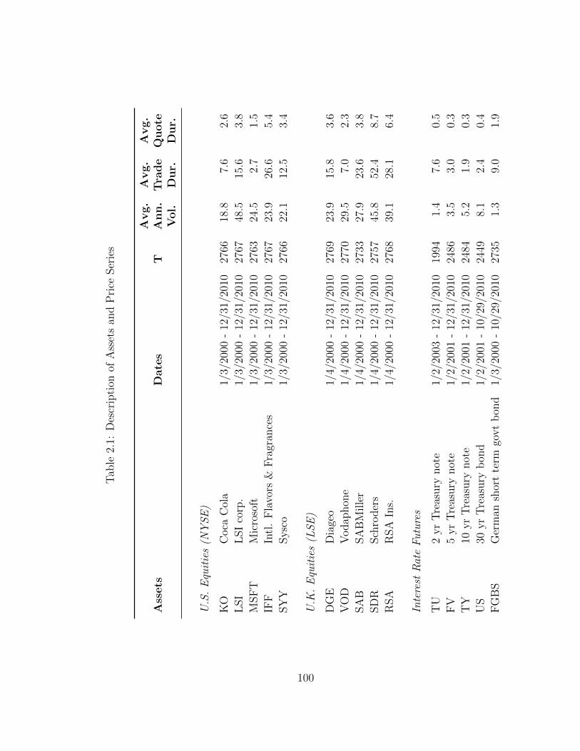
Tab
le2.
1:D
escr
ipti
onof
Ass
ets
and
Pri
ceSer
ies
Ass
ets
Date
sT
Avg.
Ann.
Vol.
Avg.
Tra
de
Du
r.
Avg.
Qu
ote
Du
r.
U.S
.E
quit
ies
(NY
SE
)
KO
Coca
Col
a1/
3/20
00-
12/3
1/20
1027
6618
.87.
62.
6
LSI
LSI
corp
.1/
3/20
00-
12/3
1/20
1027
6748
.515
.63.
8
MSF
TM
icro
soft
1/3/
2000
-12
/31/
2010
2763
24.5
2.7
1.5
IFF
Intl
.F
lavo
rs&
Fra
gran
ces
1/3/
2000
-12
/31/
2010
2767
23.9
26.6
5.4
SY
YSysc
o1/
3/20
00-
12/3
1/20
1027
6622
.112
.53.
4
U.K
.E
quit
ies
(LS
E)
DG
ED
iage
o1/
4/20
00-
12/3
1/20
1027
6923
.915
.83.
6
VO
DV
odap
hon
e1/
4/20
00-
12/3
1/20
1027
7029
.57.
02.
3
SA
BSA
BM
ille
r1/
4/20
00-
12/3
1/20
1027
3327
.923
.63.
8
SD
RSch
roder
s1/
4/20
00-
12/3
1/20
1027
5745
.852
.48.
7
RSA
RSA
Ins.
1/4/
2000
-12
/31/
2010
2768
39.1
28.1
6.4
Inte
rest
Rat
eF
utu
res
TU
2yr
Tre
asury
not
e1/
2/20
03-
12/3
1/20
1019
941.
47.
60.
5
FV
5yr
Tre
asury
not
e1/
2/20
01-
12/3
1/20
1024
863.
53.
00.
3
TY
10yr
Tre
asury
not
e1/
2/20
01-
12/3
1/20
1024
845.
21.
90.
3
US
30yr
Tre
asury
bon
d1/
2/20
01-
10/2
9/20
1024
498.
12.
40.
4
FG
BS
Ger
man
shor
tte
rmgo
vt
bon
d1/
3/20
00-
10/2
9/20
1027
351.
39.
01.
9
100
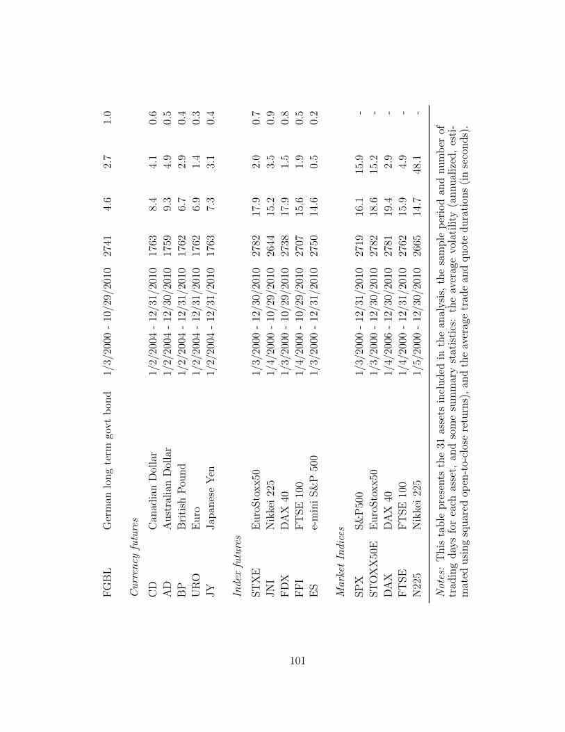
FG
BL
Ger
man
long
term
govt
bon
d1/
3/20
00-
10/2
9/20
1027
414.
62.
71.
0
Cu
rren
cyfu
ture
s
CD
Can
adia
nD
olla
r1/
2/20
04-
12/3
1/20
1017
638.
44.
10.
6
AD
Aust
ralian
Dol
lar
1/2/
2004
-12
/30/
2010
1759
9.3
4.9
0.5
BP
Bri
tish
Pou
nd
1/2/
2004
-12
/31/
2010
1762
6.7
2.9
0.4
UR
OE
uro
1/2/
2004
-12
/31/
2010
1762
6.9
1.4
0.3
JY
Jap
anes
eY
en1/
2/20
04-
12/3
1/20
1017
637.
33.
10.
4
Inde
xfu
ture
s
ST
XE
Euro
Sto
xx50
1/3/
2000
-12
/30/
2010
2782
17.9
2.0
0.7
JN
IN
ikke
i22
51/
4/20
00-
10/2
9/20
1026
4415
.23.
50.
9
FD
XD
AX
401/
3/20
00-
10/2
9/20
1027
3817
.91.
50.
8
FF
IF
TSE
100
1/4/
2000
-10
/29/
2010
2707
15.6
1.9
0.5
ES
e-m
ini
S&
P50
01/
3/20
00-
12/3
1/20
1027
5014
.60.
50.
2
Mar
ket
Indi
ces
SP
XS&
P50
01/
3/20
00-
12/3
1/20
1027
1916
.115
.9-
ST
OX
X50
EE
uro
Sto
xx50
1/3/
2000
-12
/30/
2010
2782
18.6
15.2
-
DA
XD
AX
401/
4/20
06-
12/3
0/20
1027
8119
.42.
9-
FT
SE
FT
SE
100
1/4/
2000
-12
/31/
2010
2762
15.9
4.9
-
N22
5N
ikke
i22
51/
5/20
00-
12/3
0/20
1026
6514
.748
.1-
Not
es:
This
table
pre
sents
the
31as
sets
incl
uded
inth
ean
alysi
s,th
esa
mple
per
iod
and
num
ber
oftr
adin
gday
sfo
rea
chas
set,
and
som
esu
mm
ary
stat
isti
cs:
the
aver
age
vola
tility
(annual
ized
,es
ti-
mat
edusi
ng
squar
edop
en-t
o-cl
ose
retu
rns)
,an
dth
eav
erag
etr
ade
and
quot
edura
tion
s(i
nse
conds)
.
101

Tab
le2.
2:Sum
mar
ySta
tist
ics
ofso
me
sam
ple
real
ized
mea
sure
sfo
rtw
ore
pre
senta
tive
asse
ts
mea
nst
dd
evsk
ewku
rtm
inm
axacp
1qacp
2qacp1q
acp2q
Mic
roso
ft(M
SF
T)
RV
dai
ly3.
207.
216.
5372
.09
0.00
112.
860.
260.
290.9
60.9
9R
V5m
ct3.
374.
484.
5636
.86
0.18
63.1
40.
720.
680.9
60.9
5R
V5m
ctss
3.27
4.38
4.84
44.1
70.
1771
.69
0.72
0.68
0.9
60.9
5R
V1t
bt
11.2
420
.36
3.75
20.9
60.
2720
7.58
0.94
0.92
0.9
90.9
8R
Vp
a1t
bt
3.27
4.28
5.78
71.9
50.
1986
.52
0.72
0.72
0.9
40.9
2R
Vac
11m
ct3.
404.
545.
2253
.70
0.15
81.8
90.
720.
700.9
40.9
4R
Kth
21m
bt
3.32
4.47
4.71
40.6
40.
0969
.96
0.71
0.67
0.9
50.9
5M
SR
V1m
ct3.
234.
514.
8141
.16
0.13
68.1
90.
690.
650.9
60.9
5M
LR
V5s
ct3.
213.
625.
0250
.41
0.26
63.3
20.
800.
770.9
50.9
3R
RV
m5
1mct
3.34
4.23
5.37
61.7
20.
2181
.49
0.74
0.72
0.9
40.9
3
US
D/A
UD
exch
an
gera
tefu
ture
(AD
)
RV
dai
ly0.
461.
379.
8814
9.55
0.00
28.9
50.
390.
400.9
80.9
3R
V5m
ct0.
521.
057.
9091
.46
0.04
17.2
10.
710.
780.9
40.9
3R
V5m
ctss
0.51
1.02
7.69
86.6
60.
0415
.77
0.74
0.80
0.9
20.9
1R
V1t
bt
0.70
1.04
7.61
92.7
30.
0718
.37
0.70
0.70
0.9
50.9
1R
Vp
a1t
bt
0.51
1.01
7.81
91.2
60.
0416
.70
0.76
0.79
0.9
40.9
1R
Vac
11m
ct0.
521.
027.
9596
.27
0.04
18.1
40.
730.
780.9
40.9
3R
Kth
21m
bt
0.51
1.04
8.44
107.
350.
0417
.70
0.71
0.78
0.9
20.9
0M
SR
V1m
ct0.
511.
048.
0695
.30
0.04
17.0
40.
720.
790.9
20.9
1M
LR
V5s
ct0.
570.
996.
9171
.92
0.06
16.0
60.
790.
780.9
60.9
2R
RV
m5
1mct
0.54
1.00
7.29
78.9
20.
0516
.25
0.78
0.79
0.9
50.9
1
Note
s:T
his
tab
led
isp
lays
the
sum
mar
yst
atis
tics
for
seve
ral
esti
mat
ors
for
Mic
roso
ftan
Au
stra
lian
-US
Doll
ar
futu
res.
Ref
erri
ng
toth
efo
ur
righ
t-m
ost
colu
mn
s,acppq
dec
not
esth
epth
sam
ple
auto
corr
elat
ion
,an
dacppq
den
otes
thepth
esti
mate
dau
toco
rrel
atio
nof
QV
bas
edon
are
aliz
edm
easu
re,
usi
ng
the
inst
rum
enta
lva
riab
les
met
hod
ofH
anse
nan
dL
un
de
(2010).
102

Tab
le2.
3:T
op10
Est
imat
ors
for
each
asse
tcl
ass
and
the
aver
age
rank
wit
hin
the
asse
tcl
ass
US
Equities
avgra
nk
UK
Equities
avgra
nk
Bond
Futu
res
avgra
nk
trR
Kb
art
5sb
14m
qR
Kth
25s
b6
mq
RR
Vm
55s
b29
trR
RV
m5
1mb
ss14
mq
RK
bart
5s
b8
mq
RR
Vm
55s
bss
30tr
RV
pa
1sc
15m
qR
RV
m5
1m
bss
9m
qR
RV
m10
1s
css
34
trR
Vac
11m
bss
18m
qR
Vp
a1s
b10
mq
RR
Vm
10
1s
c35
trR
Kth
25s
c18
mq
RR
Vm
51m
b12
mq
RR
Vm
10
1s
bss
36tr
RR
Vm
51m
css
19m
qR
Kn
fp1s
b12
mq
RR
Vm
55s
css
36tr
RK
bar
t5s
c20
mq
RK
bart
1s
b18
mq
RR
Vm
55s
c36
trR
RV
m5
1mb
21m
qR
V5m
bss
23
mq
RR
Vm
10
1s
b37
trR
RV
m5
1mc
21m
qR
Kcu
b1s
b24
trR
Kth
21s
c37
trR
Kth
25s
b22
mq
RV
pa
5s
b31
mq
RV
ac1
5s
c39
Assetclass
Fre
q.
No.
Freq.
No.
Fre
q.
No.
RV
05m
10
RVac1
1m1
05s
1RK
bart
5s2
1s,
5s
20
cu
bic
01s
10
th2
5s2
5s
11s
1n
fp0
1s
10
kSRV
tsrv
00
0m
srv
00
0M
LRV
00
0RRV
m=
51m
45m
25s
4m
=10
00
1s
4RVpa
1s1
1s,
5s
20
RV
incl.
PA
1s1
1s,
5s,
5m
30
103
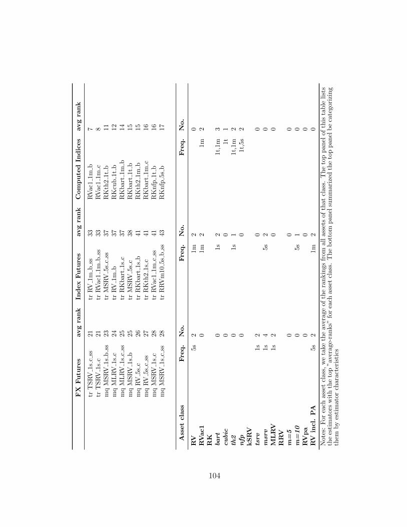
FX
Futu
res
avgra
nk
IndexFutu
res
avgra
nk
Computed
Indices
avgra
nk
trT
SR
V1s
css
21
trR
V1m
bss
33
RV
ac1
1m
b7
trT
SR
V1s
c21
trR
Vac1
1m
bss
33
RV
ac1
1m
c8
mq
MS
RV
1sb
ss23
trM
SR
V5s
css
37
RK
th2
1t
b11
mq
ML
RV
1sc
24
trR
V1m
b37
RK
cub
1t
b12
mq
ML
RV
1sc
ss25
trR
Kb
art
1s
c37
RK
bart
1m
b14
mq
MS
RV
1sb
25
trM
SR
V5s
c38
RK
bart
1t
b15
mq
RV
5sc
26
trR
Kb
art
1s
b41
RK
th2
1m
b15
mq
RV
5sc
ss27
trR
Kth
21s
c41
RK
bart
1m
c16
mq
MS
RV
1sc
28
trR
Vac1
1m
css
41
RK
nfp
1t
b16
mq
MS
RV
1sc
ss28
trR
RV
m10
5s
bss
43
RK
nfp
5s
b17
Assetclass
Fre
q.
No.
Fre
q.
No.
Fre
q.
No.
RV
5s2
1m
20
RVac1
01m
21m
2RK
bart
01s
21t,
1m
3cu
bic
00
1t
1th
20
1s
11t,
1m
2n
fp0
01t,
5s
2kSRV
tsrv
1s2
00
msr
v1s
45s
20
MLRV
1s2
00
RRV
m=
50
00
m=
10
05s
10
RVpa
00
0RV
incl.
PA
5s2
1m
20
Not
es:
For
each
asse
tcl
ass,
we
take
the
aver
age
of
the
ran
kin
gs
from
all
ass
ets
of
that
class
.T
he
top
pan
elof
this
tab
leli
sts
the
esti
mat
ors
wit
hth
eto
p”a
vera
ge-r
an
ks”
for
each
ass
etcl
ass
.T
he
bott
om
pan
elsu
mm
ari
zed
the
top
pan
elb
eca
tegori
zin
gth
emby
esti
mat
orch
ara
cter
isti
cs
104

Table 2.4: Pairwise Comparison of Realized Measures
Transaction prices vs Mid-quote prices
1t 1s 5s 1m 5m 15m
RV 69 73 69 -23 -54 -50RVss 73 69 -15 -65 -96RVpa 19 -42 -65 -88 -88 -85RVac1 0 77 50 -23 -38 -4RK 13 -35 -47 -52 -35 -13M/TSRV 21 8 -31 -67 -31 -10MLRV -31 77 23 -50 -46 4RRV 8 27 -15 -65 -96 -85BR 23
Calendar-time sampling vs Tick-time sampling
1t 1s 5s 1m 5m 15m
RV -84 -74 3 23 29RVss -84 -74 0 32 23RVpa -3 35 65 74 71RVac1 -84 -65 -3 45 29RK -9 -1 48 58 36M/TSRV -40 -35 15 37 40TSRV -35 -52 0 32 45MLRV -81 -45 6 42 19RRV -61 3 58 81 77BR 3
Not Subsampled vs Subsampled estimators
1t 1s 5s 1m 5m 15m
RV 5 7 6 29 48RVac1 -86 -46 29 84 94M/TSRV -2 0 13 40 19MLRV 0 4 10 68 77RRV -13 -32 -19 -45 -58BR 6
Not Pre-averaged RV vs Pre-averaged RV
1t 1s 5s 1m 5m 15m
RV 74 77 39 -74 -100 -100
105

Notes for Table 2.4: This table summarizes results on pairwise comparisons of
realized measures that differ only in the price series used (top panel), sampling
scheme used (middle panel), or use of subsampling or pre-averaging (bottom
two panels). For each pair, a robust t-statistic on the average loss difference is
computed per asset and estimator type. Each table cell summarizes the pair-
wise comparisons for a given estimator class and frequency by reporting the pro-
portion of significantly positive t-statistics minus the proportion of significantly
negative t-statistics. A negative value indicates that the first approach (e.g.,
calendar-time sampling in the top panel) outperforms the second approach, a
positive value indicates the opposite. Values less than -33 are dark-shaded,
and values greater than 33 are light-shaded. ‘RK’ aggregates the resulting t-
statistics from the 4 types of Realized Kernels, MSRV and TSRV results are
combined in ‘M/TSRV’, and RRVm5 and RRVm10 results are combined.
106

Tab
le2.
5:N
um
ber
ofes
tim
ator
sth
atar
esi
gnifi
cantl
ydiff
eren
tfr
omR
V5m
inin
Rom
ano-
Wol
fT
ests
Wors
eB
ett
er
QV
Pro
xy:
RV
dail
yR
V15
min
RV
5min
MS
RV
1min
RK
th2
1min
RV
dail
yR
V15
min
RV
5min
MS
RV
1m
inR
Kth
21m
inT
ota
lE
stim
ato
rs
KO
194
243
228
252
249
00
00
041
8
LSI
183
281
274
288
294
00
00
041
7
MSF
T28
429
828
730
230
40
00
00
418
IFF
148
252
268
272
265
00
00
041
3
SY
Y15
522
522
120
320
30
00
00
414
DG
E18
433
635
424
426
10
00
00
420
VO
D21
929
437
122
022
20
00
00
419
SA
B14
633
829
532
632
90
00
00
420
SD
R14
231
931
327
728
80
00
00
416
RSA
162
308
381
175
213
00
00
041
9
TU
246
191
208
179
200
00
00
041
9
FV
231
254
237
238
253
00
00
042
0
TY
224
246
230
227
241
09
2428
2342
0
US
245
263
257
260
272
00
00
041
9
FG
BL
220
289
286
287
288
00
00
042
0
FG
BS
372
386
143
379
359
00
00
042
0
CD
141
189
191
190
191
00
00
042
0
AD
126
183
186
192
193
00
00
042
0
BP
161
178
182
177
178
00
00
042
0
107
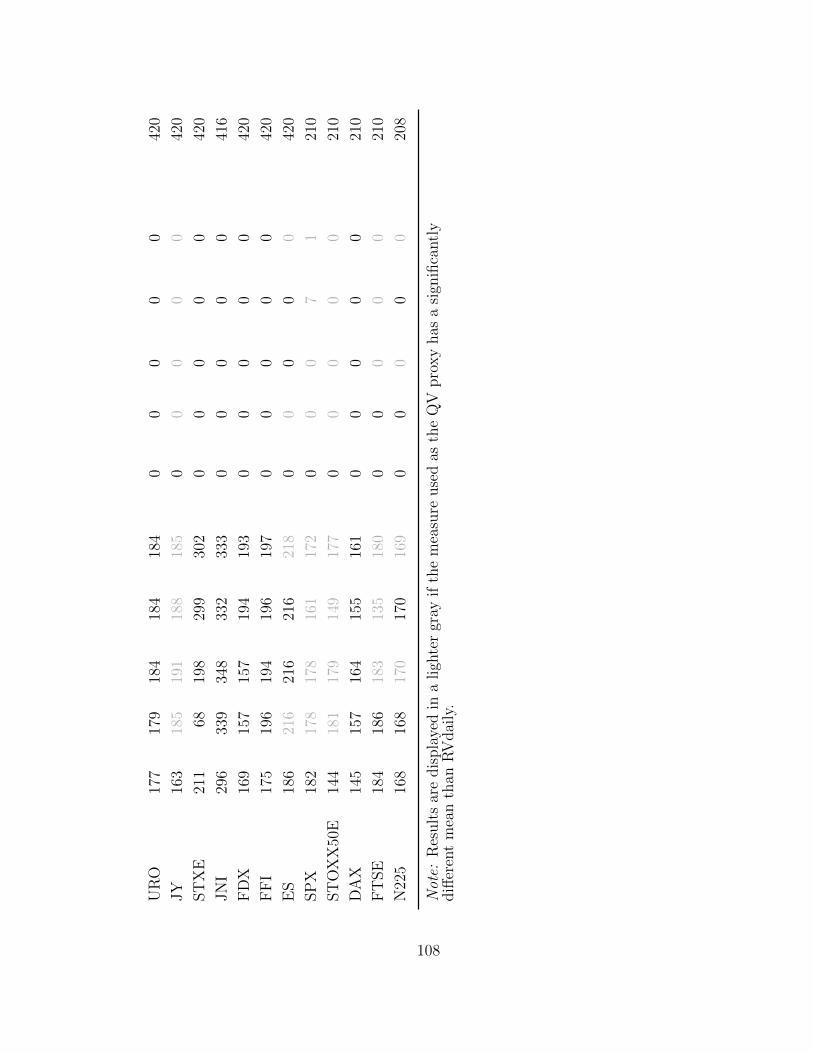
UR
O17
717
918
418
418
40
00
00
420
JY
163
185
191
188
185
00
00
042
0
ST
XE
211
6819
829
930
20
00
00
420
JN
I29
633
934
833
233
30
00
00
416
FD
X16
915
715
719
419
30
00
00
420
FF
I17
519
619
419
619
70
00
00
420
ES
186
216
216
216
218
00
00
042
0
SP
X18
217
817
816
117
20
00
71
210
ST
OX
X50
E14
418
117
914
917
70
00
00
210
DA
X14
515
716
415
516
10
00
00
210
FT
SE
184
186
183
135
180
00
00
021
0
N22
516
816
817
017
016
90
00
00
208
Not
e:R
esult
sar
edis
pla
yed
ina
ligh
ter
gray
ifth
em
easu
reuse
das
the
QV
pro
xy
has
asi
gnifi
cantl
ydiff
eren
tm
ean
than
RV
dai
ly.
108

Tab
le2.
6:P
rop
orti
onof
Rea
lize
dM
easu
res
Sig
nifi
cantl
yW
orse
than
RV
5min
All
31
Ass
ets
Inte
rest
Rate
Fu
ture
sIn
dex
Fu
ture
s
1t
1s
5s
1m
5m
15m
1t
1s
5s
1m
5m
15m
1t
1s
5s
1m
5m
15m
RV
7057
4218
1672
7558
338
5010
060
4530
030
100
RVss
5742
1818
6858
338
5410
045
300
15
90
RVpa
1816
2681
9999
3317
9210
010
010
010
520
90
100
100
RVac1
3045
3019
4973
3644
1946
8196
1035
1510
55
83
RK
1115
1850
8791
4018
5598
9997
103
1064
100
95
M/TSRV
4836
4470
9591
4217
3398
9992
5530
5079
99
95
MLRV
2843
2522
8478
3338
1783
100
8520
305
15
93
95
RRV
2535
2722
6694
1319
1350
100
9825
2815
16
79
100
BR
1831
5In
div
idu
al
Equ
itie
sC
urr
ency
Fu
ture
sC
om
pu
ted
Indic
es
1t
1s
5s
1m
5m
15m
1t
1s
5s
1m
5m
15m
1t
1s
5s
1m
5m
15m
RV
6560
5525
043
7040
100
065
100
100
100
80
080
RVss
6055
250
3540
100
065
100
100
80
40
90
RVpa
1013
055
9898
00
090
100
100
6080
40100
100
100
RVac1
4055
4314
2959
010
00
4057
8010
010
030
60
85
RK
014
328
7186
00
141
9388
565
4518
80
98
M/TSRV
5049
3952
9089
3010
3563
9889
8010
090
75
98
97
MLRV
3055
350
7161
010
00
8080
8010
010
020
85
85
RRV
2550
365
3985
00
01
5710
010
010
010
075
80
100
BR
110
75
Note
s:T
his
tab
leag
greg
ates
,fo
rgr
oup
sof
ass
ets
(eit
her
all
31
ass
ets
or
ass
ets
bel
on
gin
gto
on
ecl
ass
),th
eR
oman
o-W
olf
test
resu
lts
iden
tify
ing
esti
mat
ors
that
are
sign
ifica
ntl
yw
ors
eth
an
the
ben
chm
ark
5-m
inu
teR
V(c
ale
nd
ar-
tim
e,tr
ad
esp
rice
s)es
tim
ato
r.E
ach
tab
lece
llre
por
tsth
ep
rop
orti
onof
esti
mat
ors
of
ace
rtain
esti
mato
rcl
ass
an
dsa
mp
lin
gfr
equ
ency
(acr
oss
ass
ets,
an
dallow
ing
for
diff
eren
tsa
mp
lin
gsc
hem
esan
dsa
mp
led
pri
cese
ries
)th
at
are
fou
nd
tob
esi
gn
ifica
ntl
yw
ors
eth
an
the
ben
chm
ark
esti
mat
or
ina
Rom
an
o-W
olf
test
.
109
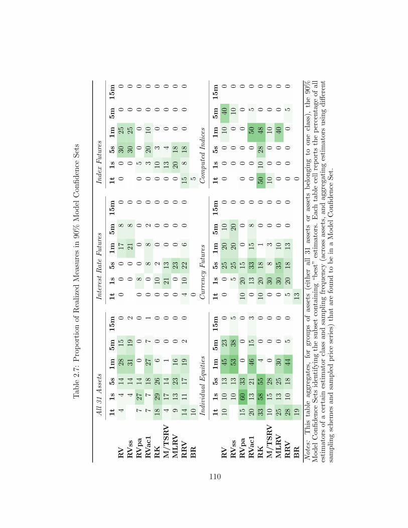
Tab
le2.
7:P
rop
orti
onof
Rea
lize
dM
easu
res
in90
%M
odel
Con
fiden
ceSet
s
All
31
Ass
ets
Inte
rest
Rate
Fu
ture
sIn
dex
Fu
ture
s
1t
1s
5s
1m
5m
15m
1t
1s
5s
1m
5m
15m
1t
1s
5s
1m
5m
15m
RV
44
1428
150
00
017
80
00
3025
00
RVss
414
3119
20
021
80
030
25
00
RVpa
727
140
00
08
00
00
05
00
00
RVac1
77
1827
71
00
88
20
03
2010
00
RK
1829
266
00
010
20
00
010
30
00
M/TSRV
417
141
00
021
130
00
013
40
00
MLRV
913
2316
00
00
230
00
020
180
00
RRV
1411
1719
20
410
226
00
158
180
00
BR
100
5In
div
idu
al
Equ
itie
sC
urr
ency
Fu
ture
sC
om
pu
ted
Indic
es
1t
1s
5s
1m
5m
15m
1t
1s
5s
1m
5m
15m
1t
1s
5s
1m
5m
15m
RV
1010
1345
230
00
2520
100
00
010
40
0RVss
1013
5338
55
2520
200
00
010
0RVpa
1560
330
00
1020
150
00
00
00
00
RVac1
2013
2146
153
013
3315
80
00
050
50
RK
3358
554
00
1020
181
00
5010
2848
00
M/TSRV
1015
280
00
030
83
00
100
010
00
MLRV
2513
2530
00
030
3510
00
00
040
00
RRV
2810
1844
50
520
1813
00
00
00
50
BR
1913
0
Note
s:T
his
tab
leag
greg
ates
,fo
rgr
oup
sof
asse
ts(e
ith
eral
l31
asse
tsor
asse
tsb
elon
gin
gto
one
class
),th
e90%
Mod
elC
onfi
den
ceS
ets
iden
tify
ing
the
sub
set
conta
inin
g“b
est”
esti
mat
ors.
Eac
hta
ble
cell
rep
orts
the
per
centa
ge
of
all
esti
mat
ors
ofa
cert
ain
esti
mat
orcl
ass
and
sam
pli
ng
freq
uen
cy(a
cros
sas
sets
,an
dag
greg
atin
ges
tim
ators
usi
ng
diff
eren
tsa
mp
lin
gsc
hem
esan
dsa
mp
led
pri
cese
ries
)th
atar
efo
un
dto
be
ina
Mod
elC
onfi
den
ceS
et.
110

Table 2.8: Conditional Relative Performance of Realized Measures and RV5min
RV5m vs.RVdaily
RV1m
MSRV5s
RVac11m
RKth25s
MLRV1s
avgdur 0.74 0.10 -0.44 -1.72 -1.57 1.28(0.01) (0.00) (-0.01) (-0.02) (-0.05) (0.02)
volm 1.55 -1.74 -1.38 -0.36 -1.24 -1.97(0.01) (-0.01) (-0.01) (0.00) (-0.01) (-0.01)
BAsprd 1.54 -1.57 -1.23 -1.78 -1.87 -2.57(0.06) (-0.04) (-0.03) (-0.03) (-0.06) (-0.06)
ac1 5s -0.70 -4.21 -1.26 -1.63 -0.56 1.65(-0.05) (-0.41) (-0.10) (-0.21) (-0.04) (0.15)
jumpprop 0.97 0.04 0.28 -0.40 1.33 -2.17(0.03) (0.00) (0.01) (-0.02) (0.05) (-0.08)
noiseratio 3.56 -8.84 -4.98 -2.71 -2.14 -13.11(0.01) (-0.05) (-0.02) (-0.03) (-0.01) (-0.06)
logQV -4.94 -2.02 -2.62 1.85 -2.11 0.91(-0.03) (-0.01) (-0.02) (0.01) (-0.01) (0.01)
equities -12.38 -0.63 0.60 0.38 4.23 -12.68(-0.12) (0.00) (0.00) (0.00) (0.03) (-0.08)
bond fut -10.26 6.34 5.90 -4.27 4.52 -0.80(-0.09) (0.17) (0.14) (-0.06) (0.08) (-0.02)
FX fut -8.59 7.39 5.74 1.20 5.94 6.71(-0.16) (0.10) (0.07) (0.02) (0.07) (0.09)
index fut -8.79 10.45 9.00 -0.47 6.79 4.49(-0.09) (0.13) (0.09) (0.00) (0.08) (0.06)
UK -0.57 -18.11 -12.96 -3.08 -7.74 -21.47(-0.01) (-0.19) (-0.11) (-0.03) (-0.07) (-0.17)
Europe 2.28 -8.31 -6.47 0.09 -4.08 -11.90(0.03) (-0.12) (-0.08) (0.00) (-0.05) (-0.17)
Asia -0.96 -7.19 -3.54 -1.52 -1.76 -16.70(-0.02) (-0.11) (-0.04) (-0.05) (-0.02) (-0.24)
Notes: Each column of this table presents the t-statistics (top) and coefficient estimates
(bottom, in parentheses) for a pooled regression of the form Lpθit,Mi0,tqLpθ
it,M
ij,tq
β1jXit1 γ1jZ
i εij,t, for t 1, 2, ...T ; i 1, 2, ...26, where M i0,t is RV5min, M i
j,t is a
competing realized measure listed in the table header, Xit1 are the set of 7 explanatory
variables listed in the first 7 rows of first column, and Zi are the set of 7 categoricalvariables listed in the last 7 rows of the first column. 26 assets (all assets other than thecomputed indices) are included in each panel regression, and T=2860 (though panel isunbalanced). All estimators are calendar-time sampled, transaction price estimators.Statistically significant results (at 5% level) are shaded.
111

Table 2.9: Proportion of RM-based HAR-RV models in 90% Model ConfidenceSets, for forecast horizons 1 through 5
All 31 Assets Interest Rate Futures
1t 1s 5s 1m 5m 15m 1t 1s 5s 1m 5m 15mRV 12 14 17 25 35 30 2 3 8 0 1 3RVss 16 16 25 35 44 5 7 1 0 0RVpa 40 34 36 41 23 15 0 0 0 4 3 8RVac1 14 18 17 29 33 27 2 5 6 0 3 1RK 33 30 34 35 30 13 0 0 1 5 6 2M/TSRV 19 17 19 31 28 11 3 7 5 0 5 4MLRV 19 18 20 33 34 11 2 8 5 0 6 0RRV 18 15 17 37 42 27 2 5 2 0 9 13BR 36 2BPV 10 13 16 25 42 49 0 0 1 2 20 34BPVpa 42 34 47 60 41 23 10 11 37 53 49 30min/medRV 11 13 15 23 38 44 0 0 1 3 22 29QRV 11 12 16 36 63 55 0 0 6 39 74 78TrunRV 11 11 22 42 61 63 0 0 4 57 72 88
Individual Equities Currency Futures
1t 1s 5s 1m 5m 15m 1t 1s 5s 1m 5m 15mRV 5 6 6 23 42 35 28 42 47 64 78 71RVss 0 5 23 43 58 40 46 63 79 73RVpa 46 35 41 49 32 17 72 70 79 69 49 39RVac1 12 5 9 31 38 35 30 52 49 71 75 47RK 40 32 37 39 35 14 68 68 74 80 62 32M/TSRV 15 11 16 32 31 10 38 46 46 77 57 30MLRV 15 5 10 35 42 11 38 52 49 80 68 33RRV 10 4 5 43 58 33 44 46 57 81 76 54BR 37 64BPV 6 2 3 16 38 49 24 43 44 72 90 86BPVpa 46 29 38 58 39 18 80 85 93 93 68 47min/medRV 7 3 3 16 32 43 26 38 44 68 84 79QRV 6 0 4 13 46 47 28 34 52 84 96 86TrunRV 7 - 0 16 39 46 30 40 53 85 91 96
Notes: This table (continued on the next page) aggregates, for groups of assets (ei-ther all 31 assets, or assets belonging to one class), the 90% Model Confidence Setsidentifying the subset containing “best” estimators. Each table cell reports the percent-age of all estimators of a certain estimator class and sampling frequency (across assets,and aggregating estimators using different sampling schemes and sampled price series)that are found to be in a Model Confidence Set. ‘-’ indicates that for the assets underconsideration, all estimators of that class and sampling frequency yield values that areunrealistically small and thus dropped from the competing set (see section 7.2 in theAppendix).
112

Index Futures
1t 1s 5s 1m 5m 15mRV 18 16 16 17 25 16RVss 17 17 17 25 33RVpa 36 30 24 32 12 5RVac1 10 18 13 19 24 17RK 28 22 29 26 21 3M/TSRV 19 14 15 20 20 3MLRV 26 18 20 24 19 6RRV 22 15 13 27 21 10BR 47BPV 4 2 22 18 32 32BPVpa 30 23 35 39 13 5min/medRV 5 6 17 16 26 31QRV 4 13 13 29 44 22TrunRV 3 1 17 30 54 39
Computed Indices
1t 1s 5s 1m 5m 15mRV 16 16 18 30 20 20RVss 0 0 34 22 54RVpa 52 40 38 58 4 0RVac1 20 13 14 32 20 34RK 26 29 29 20 24 14M/TSRV 30 13 14 24 35 4MLRV 28 13 34 32 34 0RRV 26 20 35 35 34 16BR 36BPV 32 - - 34 33 45BPVpa 56 32 40 68 12 0min/medRV 32 - 0 19 37 42QRV 32 0 12 42 78 34TrunRV 24 - 13 24 74 53
113

2.8 Figures
0 10 20 30 40 500
0.2
0.4
0.6
0.8
1All Assets
forecast horizon0 10 20 30 40 50
0
0.2
0.4
0.6
0.8
1Individual Equities
forecast horizon
0 10 20 30 40 500
0.2
0.4
0.6
0.8
1Interest Rate Futures
forecast horizon0 10 20 30 40 50
0
0.2
0.4
0.6
0.8
1Currency Futures
forecast horizon
0 10 20 30 40 500
0.2
0.4
0.6
0.8
1Index Futures
forecast horizon
Proportion of RM−based HAR−RV forecasts in 90% Model Confidence Sets
0 10 20 30 40 500
0.2
0.4
0.6
0.8
1Computed Indices
forecast horizon
Figure 2.1: This figure presents the proportion of all realized measure based HAR-RV forecasts of QV that are included in the 90% model confidence set at each forecasthorizon, ranging from 1 to 50 days. The upper left panel presents the results over all31 assets, and the remaining panels present results for each of the five asset classesseparately.
114
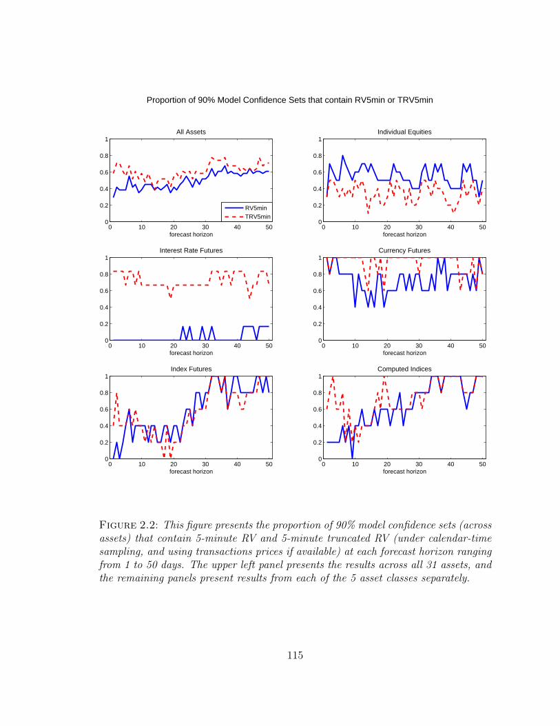
0 10 20 30 40 500
0.2
0.4
0.6
0.8
1All Assets
forecast horizon
0 10 20 30 40 500
0.2
0.4
0.6
0.8
1Individual Equities
forecast horizon
0 10 20 30 40 500
0.2
0.4
0.6
0.8
1Interest Rate Futures
forecast horizon0 10 20 30 40 50
0
0.2
0.4
0.6
0.8
1Currency Futures
forecast horizon
0 10 20 30 40 500
0.2
0.4
0.6
0.8
1Index Futures
forecast horizon
Proportion of 90% Model Confidence Sets that contain RV5min or TRV5min
0 10 20 30 40 500
0.2
0.4
0.6
0.8
1Computed Indices
forecast horizon
RV5minTRV5min
Figure 2.2: This figure presents the proportion of 90% model confidence sets (acrossassets) that contain 5-minute RV and 5-minute truncated RV (under calendar-timesampling, and using transactions prices if available) at each forecast horizon rangingfrom 1 to 50 days. The upper left panel presents the results across all 31 assets, andthe remaining panels present results from each of the 5 asset classes separately.
115

Appendix A
Appendix for Chapter 1
116

A.1 Additional Tables and Figures
Table A.1: CDS Reference Entities and their Credit Ratings
ticker reference entity sector ratings range
Investment Grade (listed in CDX.NA.IG.17)AA Alcoa Inc. basic mat. A+ ; BBB-CAG ConAgra Foods, Inc. cons. goods BBB+ ; BBBMO Altria Group, Inc. cons. goods A ; BBBWHR Whirlpool Corporation cons. goods BBB+ ; BBB-AZO Autozone, Inc. cons. services A- ; BBBSWY Safeway Inc. cons. services BBB ; BBB-YUM YUM! Brands, Inc. cons. services BBB ; BBAXP American Express Company financials A+ ; BBB+GEcc General Electric Capital Corp. financials AAA ; AA+ARW Arrow Electronics, Inc. industrials BBB+ ; BBB-CSX CSX Corporation industrials BBB ; BBB-UNP Union Pacific Corp. industrials BBB+ ; BBB-UNH Unitedhealth Group Inc. healthcare A ; A-APC Anadarko Petroleum Corp. energy BBB+ ; BBB-COP Conoco Phillips energy A ; BBBVLOC Valero Energy Corp. energy BBB ; BBB-CSC Computer Sciences Corp. technology A ; BBB+XRX Xerox Corp. technology A ; BB-COXComInc COX Communications, Inc. telecomm. BBB+ ; BBB-AEP American Electric utilities A- ; BBB
Power Company, Inc.
High Yield (listed in CDX.NA.HY.17)WY Weyerhaeuser Company basic mat. BBB ; BBB-GT The Goodyear Tire & consumer goods BB- ; B+
Rubber CompanyLTD L Brands, Inc. cons. services BBB+ ; BBRCL Royal Caribbean Cruises Ltd. cons. services BBB- ; BB-RSH Radioshack Corp. cons. services A- ; B+TSG Sabre Holdings Corp. cons. services not avail.CMS CMS Energy Corp. energy BB ; BBB-MGIC MGIC Investment Corp. financials A ; CCCTHC Tenet Healthcare Corp. healthcare B+ ; BB-AMD Advanced Micro Devices, Inc. technology B+ ; CCC+
This table lists the CDS reference entities with their sector (as listed by Markit forCDX indices) and the range of Standard & Poor’s long-term bond ratings for thesample period from December 31, 2003 to March 31, 2012. The first column displaysMarkit tickers for the reference entities.
117

Tab
leA
.2:
Sum
mar
yof
lengt
hs
and
loca
tion
sof
95%
Con
fiden
ceSet
s,α
0.10
full
sam
ple
Jan
04-
Sep
06N
ov06
-Jun
09Jul
09-
Apr
12
Pro
p.
(%)
avgCL
cente
rP
rop.
(%)
avgCL
cente
rP
rop.
(%)
avgCL
cente
rP
rop.
(%)
avgCL
cente
r
con
fide
nce
set
len
gth:
¤0.
148
0.08
560.
0733
0.10
540.
08(0
.1,0
.2]
60.
354
0.25
70.
297
0.44
(0.2
,0.4
]5
0.54
40.
455
0.49
70.
63(0
.4,0
.6]
40.
603
0.63
60.
605
0.58
(0.6
,0.8
]6
0.57
60.
538
0.58
40.
59(0
.8,1
]22
0.54
170.
5333
0.54
160.
54em
pty
8–
10–
8–
7–
test
ingL
0
0.60
:0.
60PC
L32
–25
–45
–25
–0.
60PC
L|`pCLq
0.5
4–
2–
4–
5–
0.60
PCL|`pCLq
0.2
0–
0–
0–
0–
This
table
show
sre
sult
sbas
edon
asym
pto
tic
90%
confiden
cese
tsfo
rL
GD
.T
he
confiden
cese
tsi
zes
and
loca
tion
s,an
dth
epro
por
tion
incl
udin
g0.
60ar
epre
sente
d.
For
com
par
ison
,th
ista
ble
replica
tes
the
sum
mar
ies
ofth
e95
%co
nfiden
cese
tsfo
und
inta
ble
s1.
2an
d1.
3.
118
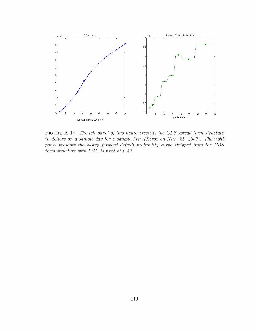
Figure A.1: The left panel of this figure presents the CDS spread term structurein dollars on a sample day for a sample firm (Xerox on Nov. 21, 2007). The rightpanel presents the 8-step forward default probability curve stripped from the CDSterm structure with LGD is fixed at 0.40.
119

Appendix B
Appendix for Chapter 2
B.1 Data Cleaning
All series were cleaned according to a set of baseline rules similar to those in Barndorff-
Nielsen et al. (2009). Using notation from that paper, these rules are:
P1 Prices out of normal business hours were discarded.
P2 Prices with a 1-tick reversal greater than 15 times the median spread were
removed.
P3 Prices were aggregated using the median of all prices with that time stamp.
Q1 Quotes with bid above offer were removed.
Q2 Quotes with a spread greater than 15 times the daily median spread were
removed
QT1 The maximum price was determined as the minimum of the maximum offer
and the maximum transaction price, plus 2 times the daily median standard
120

deviation. The minimum price was determined as the maximum of the mini-
mum bid and the minimum transaction price, minus 2 times the daily spread.
Transactions with prices outside of this range, or quotes where either price was
outside this range were removed.
QT2 Transactions with prices that were outside of the lowest bid highest and offer
over the previous 1 minute and subsequent 1 minute were removed. No action
was taken if there were no quotes during this period.
QT3 Quotes with bids above or offers below the observed trading price range over
the previous and subsequent minute were removed.
F1 The active future was chosen according to the highest transaction volume on
each trading day, with the condition that once a future has been selected, it
cannot be deselected in favor of a new contract and then reselected. To avoid
this, a unique roll date was selected by maximizing the total transaction volume
to choose a single roll date.
On the rare occasion that a problem was detected, the problematic data points
were removed manually. Manual cleaning was needed in less than 0.1% of all days.
B.2 Additional Summary Statistics and Results
This section summarizes some further summary statistics for the realized measures.
Our broad implementation of realized measures means that some questionable
estimators are included, and for some of these measures, we see unrealistic estimates
of QV (negative or zero values, for example) for several days. We use the following
simple rule to remove the worst estimators before proceeding to formal rankings and
tests: if values of the realized measure are less than a prespecified cutoff (0.0001
121

for interest rate and currency futures or 0.001 for all other assets) for more than
5% of the days in the sample, then that estimator is removed from the competing
set, and not included in any subsequent analysis. Only 12 of the 31 assets have any
realized measures removed, and the maximum number of removed measures is seven
(out of 420 measures in total). Realized measures with a small number of unrealistic
estimates are retained, and the values below the cutoff are replaced with the previous
day’s value. Table B.2 records the estimators that are removed from each competing
set for each asset according to this rule. Not surprisingly, these estimators include
many that were implemented on an inappropriate sampling frequency relative to the
frequency of the available price data.
Tables B.3 and B.4 supplement Table 2.2, providing summary statistics for each
individual asset.
Table B.5 presents information on the correlation between the estimators. As
one would expect, the majority of the remaining estimators are highly correlated.
On average, about half of the correlations are over 0.9, and about 25% are 0.95 or
higher.
Table B.6 presents correlation matrices for the ranks of individual realized mea-
sures, according to estimated accuracy, across pairs of assets in a given asset class.
These rank correlations provide insights into whether the relative performance of
realized measures is similar across assets in the same asset class.
Table B.7 lists the size of the estimated model confidence set (MCS) for each
individual asset.
Results from some robustness checks are presented in Table B.8. We conduct
Romano-Wolf tests substituting MSE loss for QLIKE loss, or replacing the random-
walk approximation for QV with an AR(1) or AR(5) approximation. Consistent with
expectations, we find similar results to our base case but with lower power: we find
122

no cases where RV5min is significantly beaten by an alternative, and the number of
cases where RV5min is identified as significantly better than an alternative drops.
Also in Table B.9, we present results from Romano-Wolf tests using two alterna-
tive QV proxies, which are the 1-day lag of RVdaily or the average of 1-day lead and
1-day lag of RVdaily. The results are very similar to using 1-day lead of RVdaily.
Tables B.10 and B.11 present some summary statistics and cross-correlation es-
timates for the conditioning variables used in the panel regressions.
123

Table B.1: Short-hand codes for estimators
Order: Class Sampling Freq. Sampling Scheme Price Series Subsampling
Classes of Realized MeasuresRV Realized VarianceRVss Subsampled Realized VarianceRVpa Pre-averaged Realized VarianceRVac1 First-order autocorrelation adjusted realized varianceRKbart Realized Kernel with flat-top Bartlett kernelRKcub Realized Kernel with flat-top cubic kernelRKth2 Realized Kernel with flat-top Tukey-Hanning2 kernelRKnfp Realized Kernel with non-flat-top Parzen kernelTSRV Two-scales realized varianceMSRV Multi-scales realized varianceMLRV Maximum-Likelihood realized varianceRRVm5 Realized range-based variance with block length 5RRVm10 Realized range-based variance with block length 10BR Realized Variance with Bandi-Russell Optimal Samplingjump-robust estimators:BPV Bipower Realized VarianceBPVpa Pre-averaged Bipower VarianceminRV MinRVmedRV MedRVQRV Quantile Realized VarianceTrunRV Truncated (Threshold) Realized Variance
Sampling Frequency1t tick-by-tick1s, 5s 1-second, 5-second1m, 5m, 15m 1-minute, 5-minute, 15-minute
Sampling Schemec calendar-time samplingb tick (business)-time sampling
Price seriest transactions pricesq midquote
Subsamplingss subsampled“blank” not subsampled
Example:RV 1m ct ss Realized variance, using 1-minute calendar time sampling
of trade prices, sub-sampled
124

Tab
leB
.2:
Non
-jum
pro
bust
esti
mat
ors
that
wer
enot
imple
men
ted
due
tohav
ing
ala
rge
num
ber
ofve
rysm
all
orneg
ativ
eva
lues
KO
MSR
V15
mct
MSR
V15
mcq
LSI
MSR
V15
mct
MSR
V15
mcq
MSR
V15
mb
q
MSF
TM
SR
V15
mct
MSR
V15
mcq
IFF
MSR
V15
mct
MSR
V15
mbt
MSR
V15
mcq
MSR
V15
mb
qM
SR
V15
mct
ssM
SR
V15
mcq
ssM
SR
V15
mb
qss
SY
YM
SR
V15
mct
MSR
V15
mbt
MSR
V15
mcq
MSR
V15
mb
qM
SR
V15
mct
ssM
SR
V15
mcq
ss
VO
DB
Rb
ccq
SD
RT
SR
V15
mbt
MSR
V15
mct
MSR
V15
mbt
MSR
V15
mct
ss
RSA
MSR
V15
mct
TU
MSR
V15
mcq
US
RV
ac1
1tbt
JN
IB
Rb
ccq
BR
bc
bq
BR
bc
cqss
BR
bc
bq
ss
N22
5M
SR
V15
mc
MSR
V15
mb
Note
s:T
his
table
list
sth
ees
tim
ator
sth
atar
ere
mov
edfr
omth
eco
mp
etin
gse
tb
efor
ep
roce
edin
gto
form
al
ran
kin
gs
and
test
s(i
.e.,
not
imp
lem
ente
d).
Th
ese
esti
mat
ors
are
iden
tifi
edu
sin
gth
efo
llow
ing
rule
:m
ore
than
5%of
the
sam
ple
day
syie
ldes
tim
ated
valu
esth
atar
ele
ssth
ana
pre
spec
ified
cuto
ff(0
.000
1fo
rin
tere
stra
tean
dcu
rren
cyfu
ture
sor
0.0
01
for
all
oth
eras
sets
).
125

Table B.3: Summary of Sample Means and Standard Deviations of Realized Mea-sures
Sample Mean Sample Standard Deviationmed std dev min max med std dev min max
KO 1.77 1.82 0.32 17.24 2.82 2.46 0.96 23.00LSI 11.46 10.73 1.07 106.98 14.64 11.94 3.12 115.60MSFT 3.08 3.78 0.84 31.34 4.19 5.14 1.59 37.90IFF 2.75 2.21 0.24 21.72 5.17 3.37 0.56 30.66SYY 2.37 2.72 0.41 24.49 3.50 4.27 0.65 37.56DGE 2.68 3.38 0.60 31.37 4.06 5.29 1.43 42.47VOD 4.37 9.23 1.38 68.50 5.64 10.20 2.28 70.50SAB 3.54 2.55 1.21 22.40 6.19 4.38 1.83 29.24SDR 8.70 6.09 0.89 47.60 17.01 10.36 1.67 70.39RSA 6.93 6.88 1.03 61.13 11.82 9.06 2.71 81.44TU 0.01 0.01 0.00 0.09 0.02 0.01 0.01 0.11FV 0.06 0.06 0.03 0.53 0.08 0.05 0.03 0.56TY 0.13 0.15 0.06 1.18 0.17 0.12 0.06 1.20US 0.32 0.39 0.14 3.22 0.39 0.29 0.13 2.73FGBL 0.09 0.11 0.03 0.95 0.08 0.08 0.03 0.73FGBS 0.01 0.02 0.00 0.09 0.02 0.72 0.01 2.47CD 0.33 0.37 0.15 3.17 0.35 0.37 0.16 3.12AD 0.50 0.56 0.19 4.74 1.00 1.06 0.39 8.72BP 0.23 0.26 0.10 2.15 0.30 0.34 0.14 2.72URO 0.24 0.27 0.11 2.30 0.26 0.28 0.10 2.25JY 0.28 0.30 0.12 2.56 0.36 0.34 0.16 2.88STXE 1.76 2.06 0.57 16.58 3.17 3.97 1.38 29.25JNI 1.15 1.73 0.42 14.03 1.72 1.84 0.55 15.03FDX 1.75 1.96 0.63 16.54 2.81 2.92 1.31 23.97FFI 1.29 1.51 0.61 12.31 2.10 2.45 0.96 19.06ES 1.26 1.93 0.58 14.64 2.65 3.43 1.17 24.14SPX 1.11 1.13 0.04 10.49 2.51 2.15 0.10 20.52STOX; 1.51 1.47 0.08 13.63 2.53 2.20 0.17 20.02DAX 1.78 1.81 0.35 16.45 3.05 2.78 1.04 24.47FTSE 1.04 1.00 0.05 9.46 2.08 1.55 0.12 14.45N225 0.91 0.66 0.02 7.67 1.44 1.13 0.04 12.51
Notes: The sample mean and standard deviation of each of the implemented realizedmeasures for all 31 assets are calculated. This table summarizes the summary statisticsby listing the median sample mean, the standard deviation of the sample means, and theminimum and maximum values of sample means for a given asset. We do the same forthe collection of approximately 648 (or 324) sample standard deviations for each asset.; STOXX50E is shortened to STOX.
126

Table B.4: Estimated autocorrelation of realized measures and quadratic variation
ac(1) ac(2) ac*(1) ac*(2)
meanstddev
RV5m
meanstddev
RV5m
meanstddev
RV5m
meanstddev
RV5m
KO 0.61 0.11 0.62 0.61 0.10 0.61 0.93 0.03 0.95 0.90 0.03 0.94LSI 0.59 0.10 0.64 0.53 0.11 0.60 0.94 0.07 0.98 0.90 0.11 0.96MSFT 0.73 0.11 0.72 0.70 0.11 0.68 0.96 0.02 0.96 0.94 0.02 0.95IFF 0.48 0.14 0.46 0.45 0.15 0.41 0.95 0.01 0.93 0.92 0.02 0.93SYY 0.56 0.08 0.57 0.52 0.11 0.53 0.91 0.03 0.91 0.88 0.04 0.90DGE 0.60 0.11 0.61 0.54 0.11 0.49 0.97 0.02 0.98 0.95 0.02 0.97VOD 0.67 0.11 0.45 0.60 0.12 0.44 0.97 0.01 0.96 0.95 0.02 0.95SAB 0.50 0.12 0.49 0.41 0.12 0.33 0.96 0.03 0.97 0.94 0.04 0.91SDR 0.48 0.11 0.59 0.38 0.09 0.48 0.93 0.03 0.95 0.91 0.04 0.94RSA 0.56 0.11 0.56 0.52 0.10 0.50 0.97 0.02 0.96 0.95 0.01 0.93TU 0.37 0.16 0.35 0.37 0.14 0.35 0.96 0.03 0.94 0.95 0.02 0.95FV 0.25 0.15 0.20 0.23 0.13 0.17 0.96 0.02 0.95 0.94 0.02 0.94TY 0.30 0.18 0.19 0.27 0.16 0.16 0.97 0.02 0.96 0.94 0.02 0.94US 0.27 0.17 0.17 0.24 0.15 0.13 0.96 0.02 0.94 0.93 0.03 0.92FGBL 0.55 0.15 0.60 0.48 0.13 0.52 0.97 0.01 0.96 0.93 0.01 0.91FGBS 0.29 0.30 0.58 0.25 0.25 0.49 0.92 0.16 0.96 0.82 0.28 0.94CD 0.70 0.11 0.68 0.67 0.10 0.68 1.00 0.02 1.00 0.98 0.01 0.97AD 0.73 0.08 0.71 0.76 0.05 0.78 0.93 0.05 0.94 0.90 0.04 0.93BP 0.75 0.10 0.71 0.72 0.08 0.70 0.99 0.01 0.99 0.98 0.01 0.98URO 0.64 0.12 0.63 0.60 0.12 0.58 0.98 0.01 0.98 0.96 0.01 0.95JY 0.54 0.13 0.50 0.44 0.12 0.40 0.95 0.01 0.95 0.91 0.02 0.93STXE 0.46 0.25 0.61 0.41 0.23 0.54 0.95 0.02 0.95 0.94 0.02 0.94JNI 0.70 0.11 0.70 0.66 0.10 0.63 0.91 0.05 0.86 0.92 0.04 0.87FDX 0.64 0.15 0.23 0.58 0.14 0.20 0.95 0.01 0.96 0.95 0.02 0.95FFI 0.72 0.09 0.71 0.69 0.07 0.65 0.95 0.02 0.97 0.94 0.01 0.94ES 0.67 0.09 0.68 0.66 0.09 0.67 0.90 0.03 0.87 0.86 0.04 0.85SPX 0.66 0.08 0.69 0.65 0.08 0.68 0.91 0.03 0.92 0.86 0.03 0.86STOX 0.67 0.09 0.57 0.63 0.07 0.57 0.94 0.03 0.90 0.93 0.03 0.89DAX 0.69 0.08 0.70 0.59 0.08 0.62 0.94 0.01 0.96 0.94 0.02 0.96FTSE 0.54 0.10 0.55 0.53 0.09 0.51 0.90 0.05 0.89 0.88 0.06 0.85N225 0.70 0.10 0.74 0.64 0.08 0.67 0.95 0.04 0.95 0.94 0.03 0.94Average 0.57 0.12 0.56 0.53 0.12 0.51 0.95 0.03 0.95 0.92 0.04 0.93
Notes: This table lists the mean and standard deviation, by asset, of sample autocor-relations of realized measures (denoted “ac”) and the estimated autocorrelation of QVbased on a realized measure (denoted “ac*”), using the instrumental variables methodof Hansen and Lunde (2010). The autocorrelation estimates for RV5min (with calendar-time sampling of transaction prices) are also presented.
127
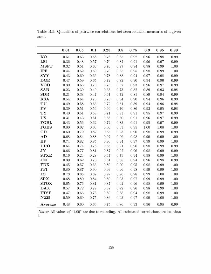
Table B.5: Quantiles of pairwise correlations between realized measures of a givenasset
0.01 0.05 0.1 0.25 0.5 0.75 0.9 0.95 0.99
KO 0.51 0.63 0.68 0.76 0.85 0.92 0.96 0.98 0.99LSI 0.36 0.48 0.57 0.70 0.82 0.91 0.96 0.97 0.99MSFT 0.32 0.51 0.63 0.76 0.87 0.94 0.98 0.99 1.00IFF 0.44 0.52 0.60 0.70 0.85 0.95 0.98 0.99 1.00SYY 0.43 0.60 0.66 0.78 0.88 0.94 0.97 0.98 0.99DGE 0.47 0.59 0.65 0.72 0.82 0.90 0.94 0.96 0.99VOD 0.39 0.65 0.70 0.78 0.87 0.93 0.96 0.97 0.99SAB 0.23 0.39 0.49 0.63 0.73 0.82 0.89 0.93 0.98SDR 0.21 0.38 0.47 0.61 0.72 0.81 0.89 0.94 0.99RSA 0.54 0.64 0.70 0.78 0.84 0.90 0.94 0.96 0.99TU 0.49 0.58 0.63 0.72 0.81 0.89 0.94 0.96 0.98FV 0.39 0.51 0.56 0.66 0.76 0.86 0.92 0.95 0.98TY 0.40 0.51 0.58 0.71 0.83 0.91 0.95 0.97 0.99US 0.31 0.43 0.51 0.65 0.80 0.91 0.96 0.97 0.99FGBL 0.43 0.56 0.62 0.72 0.83 0.91 0.95 0.97 0.99FGBS 0.00 0.02 0.03 0.06 0.63 0.95 1.00 1.00 1.00CD 0.60 0.79 0.82 0.88 0.93 0.96 0.98 0.99 0.99AD 0.68 0.84 0.88 0.92 0.96 0.98 0.99 0.99 1.00BP 0.74 0.82 0.85 0.90 0.94 0.97 0.99 0.99 1.00URO 0.64 0.74 0.78 0.86 0.91 0.96 0.98 0.99 0.99JY 0.66 0.77 0.81 0.87 0.92 0.96 0.98 0.99 0.99STXE 0.16 0.23 0.28 0.47 0.79 0.94 0.98 0.99 1.00JNI 0.39 0.62 0.70 0.81 0.88 0.94 0.96 0.98 0.99FDX 0.45 0.57 0.66 0.80 0.90 0.95 0.98 0.99 1.00FFI 0.80 0.87 0.90 0.93 0.96 0.98 0.99 0.99 1.00ES 0.73 0.83 0.87 0.92 0.96 0.98 0.99 1.00 1.00SPX 0.68 0.80 0.84 0.89 0.93 0.97 0.99 0.99 1.00STOX 0.65 0.76 0.81 0.87 0.92 0.96 0.98 0.99 1.00DAX 0.57 0.72 0.79 0.87 0.92 0.96 0.98 0.99 1.00FTSE 0.47 0.66 0.73 0.80 0.88 0.94 0.98 0.99 1.00N225 0.59 0.69 0.75 0.86 0.93 0.97 0.99 1.00 1.00
Average 0.48 0.60 0.66 0.75 0.86 0.93 0.96 0.98 0.99
Notes: All values of “1.00” are due to rounding. All estimated correlations are less than1.
128

Tab
leB
.6:
Cro
ss-a
sset
corr
elat
ions
ofra
nkin
gs
Indiv
idu
al
Equ
itie
s(a
vg
corr
:0.
70)
LSI
MSFT
IFF
SYY
DGE
VOD
SAB
SDR
RSA
KO
0.91
0.88
0.77
0.87
0.65
0.69
0.79
0.67
0.68
LSI
0.85
0.88
0.95
0.50
0.52
0.78
0.64
0.53
MSFT
0.78
0.80
0.60
0.66
0.71
0.60
0.61
IFF
0.87
0.36
0.40
0.63
0.51
0.42
SYY
0.44
0.42
0.74
0.65
0.49
DGE
0.89
0.77
0.78
0.95
VOD
0.66
0.62
0.87
SAB
0.90
0.78
SDR
0.85
Cu
rren
cyF
utu
res
(avg
corr
:0.
87)
Index
Fu
ture
s(a
vg
corr
:0.
74)
AD
BP
URO
JY
JNI
FDX
FFI
ES
CD
0.94
0.84
0.84
0.99
STXE
0.88
0.65
0.66
0.8
9AD
0.83
0.77
0.86
JNI
0.52
0.51
0.7
7BP
0.87
0.88
FDX
0.96
0.8
1URO
0.96
FFI
0.8
0
Bon
dF
utu
res
(avg
corr
:0.
84)
Com
pu
ted
Indic
es(a
vg
corr
:0.
83)
FV
TY
US
FGBL
FGBS
STOX
DAX
FTSE
N225
TU
0.96
0.90
0.87
0.83
0.70
SPX
0.97
0.79
0.94
0.7
4FV
0.96
0.91
0.88
0.64
STOX
0.80
0.96
0.7
6TY
0.91
0.93
0.60
DAX
0.83
0.8
4US
0.96
0.80
FTSE
0.7
0FGBL
0.76
Note
s:T
his
tab
led
isp
lays
ran
kco
rrel
atio
ns
ofth
era
nkin
gs(b
ased
onQ
LIK
Elo
ssfu
nct
ion
,an
dta
kin
gR
Vd
aily
asth
eQ
Vp
roxy)
acro
ssas
sets
ofth
esa
me
clas
s.
129

Table B.7: Size of 90% Model Confidence Sets
QV Proxy
Asset Total #RV
dailyRV
15minRV
5minMSRV1min
RKth21min
Estim. (a) (b) (a) (b) (a) (b) (a) (b) (a) (b)
KO 418 119 28.5 8 1.9 11 2.6 9 2.2 8 1.9LSI 417 32 7.7 11 2.6 10 2.4 4 1.0 10 2.4MSFT 418 79 18.9 6 1.4 3 0.7 5 1.2 5 1.2IFF 413 130 31.5 33 8.0 25 6.1 50 12.1 50 12.1SYY 414 148 35.7 13 3.1 20 4.8 8 1.9 10 2.4DGE 420 39 9.3 14 3.3 2 0.5 15 3.6 14 3.3VOD 419 47 11.2 6 1.4 5 1.2 4 1.0 4 1.0SAB 420 76 18.1 18 4.3 9 2.1 1 0.2 6 1.4SDR 416 24 5.8 3 0.7 1 0.2 3 0.7 4 1.0RSA 419 22 5.3 6.0 1.4 9 2.1 18 4.3 13 3.1TU 419 10 2.4 27 6.4 16 3.8 30 7.2 31 7.4FV 420 37 8.8 5 1.2 6 1.4 4 1.0 4 1.0TY 420 20 4.8 25 6.0 22 5.2 24 5.7 23 5.5US 419 8 1.9 15 3.6 6 1.4 17 4.1 10 2.4FGBL 420 3 0.7 5 1.2 4 1.0 13 3.1 10 2.4FGBS 420 39 9.3 10 2.4 2 0.5 21 5.0 15 3.6CD 420 33 7.9 10 2.4 6 1.4 6 1.4 4 1.0AD 420 135 32.1 6 1.4 5 1.2 5 1.2 9 2.1BP 420 13 3.1 20 4.8 23 5.5 9 2.1 9 2.1URO 420 9 2.1 13 3.1 6 1.4 6 1.4 6 1.4JY 420 18 4.3 16 3.8 11 2.6 16 3.8 16 3.8STXE 420 15 3.6 12 2.9 10 2.4 4 1.0 10 2.4JNI 416 15 3.6 1 0.2 2 0.5 1 0.2 1 0.2FDX 420 18 4.3 10 2.4 4 1.0 6 1.4 5 1.2FFI 420 19 4.5 7 1.7 18 4.3 17 4.0 20 4.8ES 420 34 8.1 8 1.9 13 3.1 8 1.9 1 0.2SPX 210 2 1.0 2 1.0 2 1.0 11 5.2 2 1.0STOXX50E 210 15 7.1 5 2.4 1 0.5 8 3.8 10 4.8DAX 210 20 9.5 1 0.5 2 1.0 11 5.2 7 3.3FTSE 210 17 8.1 13 6.2 13 6.2 11 5.2 11 5.2N225 208 22 10.6 6 2.9 2 1.0 5 2.4 2 1.0
Notes: Columns (a) and (b) display the number and percentage of estimators in-cluded in a 90% Model Confidence Set.
130
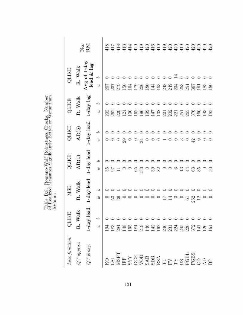
Tab
leB
.8:
Rom
ano-
Wol
fR
obust
nes
sC
hec
ks:
Num
ber
ofR
ealize
dM
easu
res
Sig
nifi
cantl
yB
ette
ror
Wor
seth
anR
V5m
in
Los
sfu
nct
ion
:Q
LIK
EM
SE
QL
IKE
QL
IKE
QL
IKE
QL
IKE
No.
RM
QV
appr
ox:
R.
Walk
R.
Walk
AR
(1)
AR
(5)
R.
Walk
R.
Walk
QV
prox
y:1-d
ay
lead
1-d
ay
lead
1-d
ay
lead
1-d
ay
lead
1-d
ay
lag
Avg
of
1-d
ay
lead
&la
g
wb
wb
wb
wb
wb
wb
KO
194
00
035
00
020
20
207
041
8L
SI
183
053
097
00
026
20
237
041
7M
SF
T28
40
390
110
00
229
027
90
418
IFF
148
00
00
029
012
40
150
041
3SY
Y15
50
00
00
00
100
016
40
414
DG
E18
40
00
650
00
162
017
90
420
VO
D21
90
00
133
034
019
60
206
041
9SA
B14
60
00
00
00
199
018
00
420
SD
R14
20
00
390
00
147
014
40
416
RSA
162
00
082
00
013
80
153
041
9T
U24
60
170
00
10
221
024
80
419
FV
231
014
00
00
020
20
249
042
0T
Y22
40
30
30
00
221
023
414
420
US
245
00
013
03
025
10
253
041
9F
GB
L22
00
610
440
00
265
025
10
420
FG
BS
372
025
20
630
420
376
036
70
420
CD
141
012
035
00
016
00
161
042
0A
D12
60
00
00
00
143
018
30
420
BP
161
00
033
00
018
30
180
042
0
131

UR
O17
70
580
30
00
160
017
30
420
JY
163
00
00
00
013
70
162
042
0ST
XE
211
016
40
320
00
241
026
10
420
JN
I29
60
450
890
00
252
031
10
416
FD
X16
90
00
420
00
186
018
00
420
FF
I17
50
580
110
00
235
020
20
420
ES
186
08
08
00
022
30
209
042
0SP
X18
20
145
012
80
00
172
018
20
210
ST
OX
X50
E14
40
00
177
00
017
10
168
021
0D
AX
145
03
014
10
20
141
015
20
210
FT
SE
184
00
017
00
00
170
018
80
210
N22
516
80
00
141
018
50
153
016
80
208
Not
es:
This
table
pre
sents
the
num
ber
ofre
aliz
edm
easu
res
that
are
sign
ifica
ntl
yb
ette
r(d
enot
edby
‘b’co
lum
ns)
orw
orse
(den
oted
by
‘w’
colu
mns)
than
the
ben
chm
ark
5-m
inute
RV
(cal
endar
-tim
esa
mpling
oftr
ansa
ctio
npri
ces)
bas
edon
five
sets
ofR
oman
o-W
olf
test
s.T
he
bas
eca
seuse
sqlike
loss
,ra
ndom
wal
kap
pro
xim
atio
nfo
rQ
V,
and
1-day
lead
ofR
Vdai
lyas
the
QV
pro
xy.
The
other
vari
atio
ns
use
MSE
loss
,an
AR
(1)
orA
R(5
)ap
pro
xim
atio
nfo
rQ
V,
and
lagg
edR
Vdai
lyor
the
aver
age
of1-
day
lagg
edan
d1-
day
lead
RV
dai
lyas
the
QV
pro
xy.
132
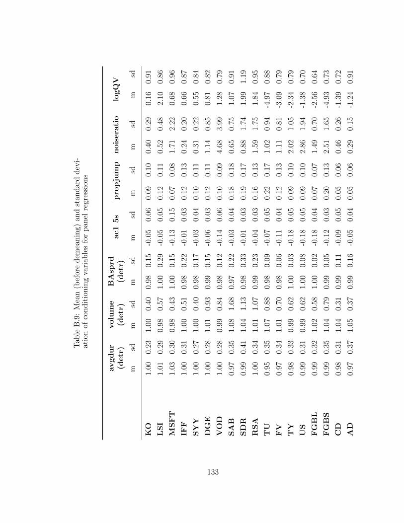
Tab
leB
.9:
Mea
n(b
efor
edem
eanin
g)an
dst
andar
ddev
i-at
ion
ofco
ndit
ionin
gva
riab
les
for
pan
elre
gres
sion
s
avgdur
(detr
)volu
me
(detr
)B
Asp
rd(d
etr
)ac1
5s
pro
pju
mp
nois
era
tio
logQ
V
msd
msd
msd
msd
msd
msd
msd
KO
1.00
0.23
1.00
0.40
0.98
0.15
-0.0
50.
060.
090.
100.
400.
290.
160.
91
LSI
1.01
0.29
0.98
0.57
1.00
0.29
-0.0
50.
050.
120.
110.
520.
482.
100.
86
MSF
T1.
030.
300.
980.
431.
000.
15-0
.13
0.15
0.07
0.08
1.71
2.22
0.68
0.96
IFF
1.00
0.31
1.00
0.51
0.98
0.22
-0.0
10.
030.
120.
130.
240.
200.
660.
87
SY
Y1.
000.
271.
000.
400.
980.
17-0
.03
0.04
0.10
0.11
0.31
0.22
0.55
0.84
DG
E1.
000.
281.
010.
930.
990.
15-0
.06
0.03
0.12
0.11
1.14
0.85
0.81
0.82
VO
D1.
000.
280.
990.
840.
980.
12-0
.14
0.06
0.10
0.09
4.68
3.99
1.28
0.79
SA
B0.
970.
351.
081.
680.
970.
22-0
.03
0.04
0.18
0.18
0.65
0.75
1.07
0.91
SD
R0.
990.
411.
041.
130.
980.
33-0
.01
0.03
0.19
0.17
0.88
1.74
1.99
1.19
RSA
1.00
0.34
1.01
1.07
0.99
0.23
-0.0
40.
030.
160.
131.
591.
751.
840.
95
TU
0.95
0.35
1.07
0.88
0.98
0.09
-0.0
70.
050.
220.
171.
020.
94-4
.97
0.88
FV
0.97
0.34
1.01
0.70
0.98
0.06
-0.1
10.
040.
120.
131.
110.
81-3
.09
0.79
TY
0.98
0.33
0.99
0.62
1.00
0.03
-0.1
80.
050.
090.
102.
021.
05-2
.34
0.79
US
0.99
0.31
0.99
0.62
1.00
0.08
-0.1
80.
050.
090.
102.
861.
94-1
.38
0.70
FG
BL
0.99
0.32
1.02
0.58
1.00
0.02
-0.1
80.
040.
070.
071.
490.
70-2
.56
0.64
FG
BS
0.99
0.35
1.04
0.79
0.99
0.05
-0.1
20.
030.
200.
132.
511.
65-4
.93
0.73
CD
0.98
0.31
1.04
0.31
0.99
0.11
-0.0
90.
050.
050.
060.
460.
26-1
.39
0.72
AD
0.97
0.37
1.05
0.37
0.99
0.16
-0.0
50.
040.
050.
060.
290.
15-1
.24
0.91
133

BP
0.98
0.32
1.04
0.34
0.99
0.13
-0.0
50.
050.
050.
060.
280.
15-1
.87
0.81
UR
O0.
990.
341.
030.
341.
000.
07-0
.11
0.05
0.04
0.06
0.95
0.42
-1.7
70.
78
JY
0.98
0.38
1.06
0.88
0.99
0.07
-0.0
70.
050.
050.
060.
530.
28-1
.64
0.77
ST
XE
0.99
0.29
1.04
0.41
1.00
0.08
-0.1
90.
070.
060.
071.
821.
180.
030.
97
JN
I1.
000.
291.
010.
311.
010.
07-0
.22
0.06
0.13
0.13
4.26
2.32
-0.0
70.
69
FD
X0.
990.
291.
020.
451.
000.
14-0
.08
0.04
0.05
0.06
0.52
0.30
0.01
1.01
FF
I0.
990.
321.
020.
460.
990.
12-0
.07
0.04
0.04
0.06
0.39
0.16
-0.2
91.
00
ES
1.00
0.37
1.03
0.30
1.00
0.07
-0.2
00.
100.
040.
064.
492.
24-0
.36
0.97
SP
X1.
000.
02–
––
–0.
000.
000.
190.
160.
370.
06-0
.41
1.00
ST
OX
X50E
1.00
0.01
––
––
0.00
0.00
0.17
0.16
0.38
0.12
-0.0
81.
02
DA
X0.
980.
13–
––
–0.
050.
070.
140.
140.
390.
120.
091.
03
FT
SE
0.98
0.14
––
––
0.03
0.09
0.17
0.16
0.36
0.21
-0.4
71.
01
N225
0.99
0.09
––
––
0.00
0.00
0.16
0.14
0.37
0.13
-0.3
30.
81
aver
age
0.99
0.28
1.02
0.63
0.99
0.13
-0.0
80.
050.
110.
111.
260.
89-0
.58
0.87
Not
es:
This
table
pre
sents
sam
ple
mea
ns
(bef
ore
dem
eanin
gfo
rth
epan
elre
gres
sion
)an
dst
andar
ddev
iati
ons
ofth
ew
inso
rize
d(t
opan
db
otto
m0.
005)
condit
ionin
gva
riab
les
use
din
the
pan
elre
gres
sion
sin
Sec
tion
5.5,
per
asse
t.A
vgd
ur
(ave
rage
dura
tion
),vo
lum
e(t
rade
volu
me)
,an
dB
Asp
rd(b
id-a
sksp
read
)ar
edet
rended
by
div
idin
gby
the
mea
nof
the
pas
t60
day
s’va
lues
.P
rop
jum
p(p
rop
orti
onof
QV
attr
ibuta
ble
toju
mps)
,noi
sera
tio
(per
trad
era
tio
ofnoi
seva
rian
ceto
QV
),an
dlo
gQV
(vol
atilit
ym
easu
re,usi
ng
subsa
mple
d5-
min
ute
RV
asQ
Vm
easu
re)
are
not
det
rended
inan
yw
ay.
Bef
ore
ente
ring
the
pan
elre
gres
sion
,al
lco
ndit
ionin
gva
riab
les
are
de-
mea
ned
usi
ng
the
full
sam
ple
aver
ages
that
app
ear
inth
ista
ble
.R
egre
ssio
nre
sult
sar
eav
aila
ble
inT
able
8.
134

Tab
leB
.10:
Cro
ss-c
orre
lati
ons
ofco
ndit
ionin
gva
riab
les,
aver
aged
over
all
31as
sets
avgd
ur(
det
r)vo
lm(d
etr)
BA
sprd
(det
r)ac
15s
pro
pju
mp
noi
sera
tio
logQ
V
avgd
ur(
det
r)1
-0.6
6-0
.03
0.01
0.07
0.06
-0.3
2
volm
(det
r)1
-0.0
2-0
.02
-0.0
4-0
.03
0.29
BA
sprd
(det
r)1
0.05
-0.0
3-0
.05
0.29
ac1
5s1
0.00
-0.3
30.
22
pro
pju
mp
10.
13-0
.07
noi
sera
tio
1-0
.25
logQ
V1
Not
es:
This
table
pre
sents
aver
age
cros
s-co
rrel
atio
ns
(ave
rage
dov
erva
lues
from
all31
asse
ts)
bet
wee
nth
ew
inso
rize
d(t
opan
db
otto
m0.
005)
condit
ionin
gva
riab
les
use
din
the
pan
elre
gres
sion
sin
Sec
tion
5.5,
per
asse
t.A
vgd
ur
(ave
rage
dura
tion
),vo
lm(t
rade
volu
me)
,an
dB
Asp
rd(b
id-a
sksp
read
)ar
ede-
tren
ded
by
div
idin
gby
the
mea
nof
the
pas
t60
day
s’va
lues
.P
rop
jum
p(p
rop
orti
onof
QV
attr
ibuta
ble
toju
mps)
,noi
sera
tio
(per
trad
era
tio
ofnoi
seva
rian
ceto
QV
),an
dlo
gQV
(vol
atilit
ym
easu
re,
usi
ng
subsa
mple
d5-
min
ute
RV
asQ
Vm
easu
re)
are
not
det
rended
.R
egre
ssio
nre
sult
sar
eav
aila
ble
inT
able
8.
135
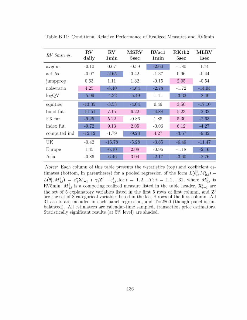
Table B.11: Conditional Relative Performance of Realized Measures and RV5min
RV 5min vs.RV
dailyRV
1minMSRV
5secRVac11min
RKth25sec
MLRV1sec
avgdur -0.10 0.67 -0.59 -2.60 -1.80 1.74
ac1 5s -0.07 -2.65 0.42 -1.37 0.96 -0.44
jumpprop 0.63 1.11 1.32 -0.15 2.05 -0.54
noiseratio 4.25 -8.40 -4.64 -2.78 -1.72 -14.04
logQV -5.99 -4.32 -5.49 1.41 -3.32 -2.40
equities -13.35 -3.53 -4.04 0.49 3.50 -17.10
bond fut -11.51 7.15 6.22 -4.88 5.23 -2.32
FX fut -9.25 5.22 -0.86 1.85 5.30 -2.63
index fut -9.72 9.13 2.05 -0.06 6.12 -4.27
computed ind. -12.12 -1.79 -9.23 4.27 -3.67 -9.02
UK -0.42 -15.78 -5.28 -3.65 -6.49 -11.47
Europe 1.45 -6.10 2.08 -0.96 -1.18 -2.16
Asia -0.86 -6.46 3.04 -2.17 -3.60 -2.76
Notes: Each column of this table presents the t-statistics (top) and coefficient es-
timates (bottom, in parentheses) for a pooled regression of the form Lpθit,M i0,tq
Lpθit,M ij,tq β1jX
it1 γ1jZ
i εij,t, for t 1, 2, ...T ; i 1, 2, ...31, where M i0,t is
RV5min, M ij,t is a competing realized measure listed in the table header, Xi
t1 are
the set of 5 explanatory variables listed in the first 5 rows of first column, and Zi
are the set of 8 categorical variables listed in the last 8 rows of the first column. All31 assets are included in each panel regression, and T=2860 (though panel is un-balanced). All estimators are calendar-time sampled, transaction price estimators.Statistically significant results (at 5% level) are shaded.
136

Bibliography
Aıt-Sahalia, Y. and Jacod, J. (2014), High-Frequency Financial Econometrics,Princeton University Press, New Jersey.
Aıt-Sahalia, Y. and Yu, J. (2009), “High frequency market microstructure noiseestimates and liquidity measures,” Annals of Applied Statistics, 3, 422–457.
Aıt-Sahalia, Y., Mykland, P. A., and Zhang, L. (2005), “How often to sample acontinuous-time process in the presence of market microstructure noise,” Reviewof Financial Studies, 18, 351–416.
Alizadeh, S., Brandt, M. W., and Diebold, F. X. (2002), “Range-Based Estimationof Stochastic Volatility Models,” Journal of Finance, 57, 1047–1092.
Andersen, T., Bollerslev, T., Diebold, F., and Ebens, H. (2001a), “The distributionof realized stock return volatility,” Journal of Financial Economics, 61, 43–76.
Andersen, T., Dobrev, D., and Schaumburg, E. (2012), “Jump-robust volatility esti-mation using nearest neighbor truncation,” Journal of Econometrics, 169, 75–93.
Andersen, T. G. and Bollerslev, T. (1998), “Answering the Skeptics: yes, standardvolatility models do provide accurate forecasts,” International Economic Review,39, 885–905.
Andersen, T. G., Bollerslev, T., Diebold, F. X., and Labys, P. (2001b), “The dis-tribution of realized exchange rate volatility,” Journal of the American StatisticalAssociation, 96, 42–55.
Andersen, T. G., Bollerslev, T., and Meddahi, N. (2005), “Correcting the Errors:Volatility Forecast Evaluation Using High-Frequency Data and Realized Volatili-ties,” Econometrica, 73, 279–296.
Andersen, T. G., Bollerslev, T., Christoffersen, P., and Diebold., F. X. (2006),“Volatility and Correlation Forecasting,” in Handbook of Economic Forecasting,Volume 1, eds. G. Elliott, C. W. J. Granger, and A. Timmermann, Elsevier, Ox-ford.
137

Andersen, T. G., Bollerslev, T., and Diebold, F. X. (2007), “Roughing it up: In-cluding jump components in the measurement, modeling and forecasting of returnvolatility,” Review of Economics and Statistics, 89, 701–720.
Andrews, D. W. and Cheng, X. (2012), “Estimation and Inference With Weak, Semi-Strong, and Strong Identification,” Econometrica, 80, 2153–2211.
Annaert, J., Claes, A. G., De Ceuster, M. J., and Zhang, H. (2013), “Estimatingthe spot rate curve using the Nelson–Siegel model: A ridge regression approach,”International Review of Economics & Finance, 27, 482–496.
Bai, J., Collin-Dufresne, P., Goldstein, R. S., and Helwege, J. (2013), “On boundingcredit event risk premia,” Working Paper.
Bandi, F. M. and Russell, J. R. (2008), “Microstructure noise, realized variance, andoptimal sampling,” Review of Economic Studies, 75, 339–369.
Barclays Capital (2010), “Standard Corporate CDS Handbook,” .
Barndorff-Nielsen, O. and Shephard, N. (2006), “Econometrics of testing for jumps infinancial economics using bipower variation,” Journal of Financial Econometrics,4, 1–30.
Barndorff-Nielsen, O. E. (2002), “Econometric analysis of realized volatility and itsuse in estimating stochastic volatility models,” Journal of the Royal StatisticalSociety: Series B (Statistical Methodology), 64, 253–280.
Barndorff-Nielsen, O. E. and Shephard, N. (2007), “Variation, jumps, market fric-tions and high frequency data in financial econometrics,” in Advances in eco-nomics and econometrics. Theory and applications, eds. R. Blundell, P. Torsten,and W. K. Newey, Econometric Society monographs, pp. 328–372, CambridgeUniversity Press, Cambridge.
Barndorff-Nielsen, O. E., Hansen, P. R., Lunde, A., and Shephard, N. (2008), “De-signing realized kernels to measure the ex post variation of equity prices in thepresence of noise,” Econometrica, 76, 1481–1536.
Barndorff-Nielsen, O. E., Hansen, P. R., Lunde, A., and Shephard, N. (2009), “Re-alized kernels in practice: trades and quotes,” Econometrics Journal, 12, C1–C32.
Barndorff-Nielsen, O. E., Hansen, P. R., Lunde, A., and Shephard, N. (2011), “Sub-sampling realised kernels,” Journal of Econometrics, 160, 204–219.
Berndt, A., Jarrow, R. A., and Kang, C. (2007), “Restructuring risk in credit defaultswaps: An empirical analysis,” Stochastic Processes and their applications, 117,1724–1749.
138

Berndt, A., Douglas, R., Duffie, D., Ferguson, M., and Schranz, D. (2008), “Mea-suring default risk premia from default swap rates and EDFs,” Tepper School ofBusiness Working Paper, p. 49.
Bibinger, M., Hautsch, N., Malec, P., and Reiss, M. (2014), “Estimating thequadratic covariation matrix from noisy observations: local method of momentsand efficiency,” Annals of Statistics, 42, 80–114.
Bollerslev, T., Engle, R. F., and Nelson, D. B. (1994), “ARCH models,” Handbookof Econometrics, 4, 2959–3038.
Canova, F. and Sala, L. (2009), “Back to square one: identification issues in DSGEmodels,” Journal of Monetary Economics, 56, 431–449.
Christensen, J. H. E. (2005), “Joint estimation of default and recovery risk: A sim-ulation study,” Tech. rep.
Christensen, J. H. E. (2007), “Joint default and recovery risk estimation: an appli-cation to CDS data,” Tech. rep.
Christensen, K. and Podolskij, M. (2007), “Realized range-based estimation of inte-grated variance,” Journal of Econometrics, 141, 323–349.
Christensen, K., Oomen, R., and Podolskij, M. (2010), “Realised quantile-basedestimation of the integrated variance,” Journal of Econometrics, 159, 74–98.
Christensen, K., Oomen, R. C., and Podolskij, M. (2014), “Fact or friction: Jumpsat ultra high frequency,” Journal of Financial Economics, 114, 576 – 599.
Conrad, J., Dittmar, R. F., and Hameed, A. (2013), “Cross-Market and Cross-FirmEffects in Implied Default Probabilities and Recovery Values,” Working Paper.
Corsi, F. (2009), “A simple approximate long-memory model of realized volatility,”Journal of Financial Econometrics, 7, 174–196.
Corsi, F., Pirino, P., and Reno, R. (2010), “Threshold bipower variation and theimpact of jumps on volatility forecasting,” Journal of Econometrics, 159, 276–288.
Das, S. R. and Hanouna, P. (2009), “Implied recovery,” Journal of Economic Dy-namics and Control, 33, 1837–1857.
Diebold, F. and Mariano, R. (2002), “Comparing predictive accuracy,” Journal ofBusiness & Economic Statistics, 20, 134–144.
Diebold, F. X. and Li, C. (2006), “Forecasting the term structure of governmentbond yields,” Journal of econometrics, 130, 337–364.
139

Driessen, J. (2005), “Is default event risk priced in corporate bonds?” Review ofFinancial Studies, 18, 165–195.
Driscoll, J. C. and Kraay, A. C. (1998), “Consistent covariance matrix estimationwith spatially dependent panel data,” Review of Economics and Statistics, 80,549–560.
Duffie, D. (1998), “Defaultable term structure models with fractional recovery ofpar,” Graduate School of Business, Stanford University.
Duffie, D. and Singleton, K. J. (1999), “Modeling term structures of defaultablebonds,” Review of Financial studies, 12, 687–720.
Elkamhi, R., Jacobs, K., and Pan, X. (2010), “The Cross-Section of Recovery Ratesand Default Probabilities Implied by Credit Default Swap Spreads,” Journal ofFinancial and Quantitative Analysis, pp. 1–51.
French, K. R., Schwert, G. W., and Stambaugh, R. F. (1987), “Expected stockreturns and volatility,” Journal of Financial Economics, 19, 3–29.
Gatheral, J. and Oomen, R. C. A. (2010), “Zero-intelligence realized variance esti-mation,” Finance and Stochastics, 14, 249–283.
Giacomini, R. and White, H. (2006), “Tests of conditional predictive ability,” Econo-metrica, 74, 1545–1578.
Guha, R. and Sbuelz, A. (2005), “Structural recovery of face value at default,” SSRNWorking Paper.
Hansen, L. P. (1982), “Large sample properties of generalized method of momentsestimators,” Econometrica: Journal of the Econometric Society, pp. 1029–1054.
Hansen, P. (2005), “A test for superior predictive ability,” Journal of Business &Economic Statistics, 23, 365–380.
Hansen, P. and Lunde, A. (2005), “A forecast comparison of volatility models: doesanything beat a GARCH(1, 1)?” Journal of Applied Econometrics, 20, 873–889.
Hansen, P. and Lunde, A. (2006a), “Consistent ranking of volatility models,” Journalof Econometrics, 131, 97–121.
Hansen, P. and Lunde, A. (2014), “Estimating the persistence and the autocorrela-tion function of a time series that is measured with error,” Econometric Theory,30, 60–93.
Hansen, P. R. and Lunde, A. (2006b), “Realized variance and market microstructurenoise,” Journal of Business & Economic Statistics, 24, 127–161.
140

Hansen, P. R., Lunde, A., and Nason, J. M. (2011), “The model confidence set,”Econometrica, 79, 453–497.
Hautsch, N. and Podolskij, M. (2013), “Preaveraging-based estimation of quadraticvariation in the presence of noise and jumps: Theory, implementation, and empir-ical evidence,” Journal of Business & Economic Statistics, 31, 165–183.
Hoechle, D. (2007), “Robust standard errors for panel regressions with cross-sectionaldependence,” Stata Journal, 7, 281.
Houweling, P. and Vorst, T. (2005), “Pricing default swaps: Empirical evidence,”Journal of International Money and Finance, 24, 1200–1225.
Jacod, J. and Todorov, V. (2014), “Efficient estimation of integrated volatility inpresence of infinite variation jumps,” Annals of Statistics, 42, 1029–1069.
Jacod, J., Li, Y., Mykland, P. A., Podolskij, M., and Vetter, M. (2009), “Microstruc-ture noise in the continuous case: the pre-averaging approach,” Stochastic Pro-cesses and their Applications, 119, 2249–2276.
Le, A. (2007), “Separating the components of default risk: A derivative-based ap-proach,” Working Paper.
Longstaff, F. A., Mithal, S., and Neis, E. (2005), “Corporate yield spreads: Defaultrisk or liquidity? New evidence from the credit default swap market,” The Journalof Finance, 60, 2213–2253.
Madan, D. B., Bakshi, G., and Zhang, F. X. (2006), “Understanding the role of re-covery in default risk models: Empirical comparisons and implied recovery rates,”Working Paper.
Mancini, C. (2001), “Disentangling the jumps of the diffusion in a geometric jumpingBrownian motion,” Giornale dellIstituto Italiano degli Attuari, 64, 19–47.
Mancini, C. (2009), “Non-parametric Threshold Estimation for Models with Stochas-tic Diffusion Coefficient and Jumps,” Scandinavian Journal of Statistics, 36, 270–296.
Markit Group Ltd. (2010), “Markit.com User Guide: CDS & Bonds,” .
Martens, M. and Van Dijk, D. (2007), “Measuring volatility with the realized range,”Journal of Econometrics, 138, 181–207.
Meddahi, N. (2003), “ARMA representation of integrated and realized variances,”Econometrics Journal, 6, 335–356.
Meddahi, N., Mykland, P., and Shephard, N. editors. (2011), “Special issue onrealised volatility,” Journal of Econometrics, 160.
141

Merton, R. C. (1974), “On the pricing of corporate debt: The risk structure ofinterest rates*,” The Journal of Finance, 29, 449–470.
Nason, J. M. and Smith, G. W. (2008), “Identifying the new Keynesian Phillipscurve,” Journal of Applied Econometrics, 23, 525–551.
Nelson, C. R. and Siegel, A. F. (1987), “Parsimonious modeling of yield curves,”Journal of business, pp. 473–489.
Oomen, R. C. A. (2006a), “Comment,” Journal of Business & Economic Statistics,24, 195–202.
Oomen, R. C. A. (2006b), “Properties of realized variance under alternative samplingschemes,” Journal of Business and Economic Statistics, 24, 219–237.
Pan, J. and Singleton, K. J. (2008), “Default and recovery implicit in the termstructure of sovereign CDS spreads,” The Journal of Finance, 63, 2345–2384.
Papke, L. E. and Wooldridge, J. M. (2008), “Panel data methods for fractionalresponse variables with an application to test pass rates,” Journal of Econometrics,145, 121–133.
Parkinson, M. (1980), “The Extreme Value Method for Estimating the Variance ofthe Rate of Return,” Journal of Business, 53, 61–65.
Patton, A. J. (2011a), “Data-based ranking of realised volatility estimators,” Journalof Econometrics, 161, 284–303.
Patton, A. J. (2011b), “Volatility forecast comparison using imperfect volatility prox-ies,” Journal of Econometrics, 160, 246–256.
Patton, A. J. and Sheppard, K. (2009a), “Evaluating Volatility and CorrelationForecasts,” in Handbook of Financial Time Series, eds. T. G. Andersen, R. A.Davis, J.-P. Kreiss, and T. Mikosch, Springer, Verlag.
Patton, A. J. and Sheppard, K. (2009b), “Optimal combinations of realised volatilityestimators,” International Journal of Forecasting, 25, 218–238.
Patton, A. J. and Sheppard, K. (2013), “Good Volatility, Bad Volatility: SignedJumps and the Persistence of Volatility,” Review of Economics & Statistics, Forth-coming.
Podolskij, M. and Vetter, M. (2009a), “Bipower-type estimation in a noisy diffusionsetting,” Stochastic processes and their applications, 119, 2803–2831.
Podolskij, M. and Vetter, M. (2009b), “Estimation of volatility functionals in thesimultaneous presence of microstructure noise and jumps,” Bernoulli, 15, 634–658.
142

Politis, D. N. and Romano, J. P. (1994), “The stationary bootstrap,” Journal of theAmerican Statistical Association, 89, 1303–1313.
Romano, J. P. and Wolf, M. (2005), “Stepwise multiple testing as formalized datasnooping,” Econometrica, 73, 1237–1282.
Schlafer, T. and Uhrig-Homburg, M. (2014), “Is recovery risk priced?” Journal ofBanking & Finance, 40, 257–270.
Schneider, P., Sogner, L., and Veza, T. (2011), “The Economic Role of Jumps andRecovery Rates in the Market for Corporate Default Risk,” Journal of Financialand Quantitative Analysis, 45, 1517–1547.
Song, J. (2007), “Loss given default implied by cross-sectional no arbitrage,” WorkingPaper.
Stock, J. H. and Wright, J. H. (2000), “GMM with weak identification,” Economet-rica, 68, 1055–1096.
Vogelsang, T. J. (2012), “Heteroskedasticity, autocorrelation, and spatial correlationrobust inference in linear panel models with fixed-effects,” Journal of Economet-rics, 166, 303–319.
White, H. (2000), “A reality check for data snooping,” Econometrica, 68, 1097–1126.
Zhang, L. (2006), “Efficient estimation of stochastic volatility using noisy observa-tions: A multi-scale approach,” Bernoulli, 12, 1019–1043.
Zhang, L., Mykland, P. A., and Aıt-Sahalia, Y. (2005), “A tale of two time scales:Determining Integrated Volatility With Noisy High-Frequency Data,” Journal ofthe American Statistical Association, 100, 1394–1411.
Zhou, B. (1996), “High-frequency data and volatility in foreign-exchange rates,”Journal of Business & Economic Statistics, 14, 45–52.
143

Biography
Lily Yanli Liu was born on October 28, 1986 in Jinan, China. She spent most of
her childhood in Burnaby, British Columbia and Lethbridge, Alberta. She attended
the University of Pennsylvania and graduated in 2008 with a Bachelor of Arts in
Economics and Mathematics. She also completed a Master of Science degree in
statistics from the University of Toronto in 2009 before beginning the PhD program
in economics at Duke University. After graduating in May 2015, Lily will join the
Federal Reserve Bank of Boston as a financial economist.
144