essays on applied econometrics - auburn university
TRANSCRIPT
Essays on Applied Econometrics
by
Ferhat Citak
A dissertation submitted to the Graduate Faculty of
Auburn University
in partial fulfillment of the
requirements for the Degree of
Doctor of Philosophy
Auburn, Alabama
August 5, 2017
Keywords: Foreign Direct Investment; Bound Testing Approach; Poverty; Education; Tourism,
Exchange rate; J-Curve
Copyright 2017 by Ferhat Citak
Approved by
Patricia A. Duffy, Chair, Affiliate Professor of Agricultural Economics and Rural Sociology
Norbert Wilson, Co-chair, Professor of Agricultural Economics and Rural Sociology
Curtis M. Jolly, Barkley Endowed Professor Emeritus
Ash Abebe, Professor of Mathematics and Statistics

ii
Abstract
This dissertation consists of three essays. The first essay analyzes the determinants of
Foreign Direct Investment (FDI) in the food products sector in Turkey. An Autoregressive
Distributed Lag (ARDL) model which is originally proposed by Pesaran and Shin (1999) and
popularized by Pesaran et al. (2001) is applied to the monthly data over the period of January,
2009, to December, 2016. In the model, FDI inflows are modeled as a function of degree of
openness, exchange rate, export price, and wage rate. The empirical results confirm there is
evidence of a long-run equilibrium relationship among these variables in Turkey. Findings
indicate that degree of openness, and export price have a positive sign and are statistically
significant, while the wage rate presents a negative sign and is statistically significant. Finally,
the cumulative sum (CUSUM) and the cumulative sum of squares (CUSUMQ) stability tests are
employed to check the stability of short-run and long-run coefficients in the ARDL error
correction model, and the results confirm that the model is structurally stable.
Essay 2 examines the relationship between the exchange rate and tourism trade balance in
Turkey from year 1970 to 2016 by applying three Vector autoregression (VAR) models. The
main findings of this paper can be documented as follows: (i) there is no long-run co-integration
relationship among the variables (ii) the reaction of the export revenue to an unexpected 1%
depreciation exchange rate shock is positive and statistically significant at the 95% level (iii) the
import tourism spending exhibits a robust significant positive response to home demand shock

iii
(iv) the response of trade balance to 1% shock in exchange rate is negative and significant, which
shows the evidence of J-curve behavior for the selected eight European countries
The final essay uses household survey data to analyze the relationship between education
and poverty in Turkey. To obtain robust estimates of the determinants of household poverty, we
applied five different econometric techniques, each relying on a different set of assumptions.
such as Ordinary Least Squares (OLS), Linear Probability Model (LPM), Probit and Logit
Models, and Instrumental Variable (IV) Probit Model. Both Ordinary Least Squares (OLS) and
Linear Probability Model (LPM) model show that the level of education, being female and
married, having a job or being retired are the important factors in determining the household
head’s poverty conditions. However, employing probit and logit models, the results from the
analysis provide evidence that married head of households are significantly more likely to poor
than single head of households. In addition, the probability of being poor decreases with the
household head’s educational attainment. However, based on the findings from Instrumental
Variable (IV) Probit model, the policy reform, which was implemented in 1961, only increases
the household head’s years of education for rural residents. Further, the higher the level of
education of the household head, the higher the household per capita income.

iv
Acknowledgments
I am graduating with the Doctorate of Philosophy degree, and I have completed several
research papers some of which are presented in this dissertation. However, none of these would
have been possible without the help of very wonderful people.
First, I would like to thank my advisor, dissertation committee chair, Dr. Patricia Duffy,
for her patient and constructive guidance on academic work, for her expertise and for her
continuous support. I also thank the other members of my dissertation committee, Dr. Norbert
Wilson, Dr. Curtis Jolly, and Dr.Ash Abebe for everything they did to help me throughout my
time at Auburn. I am also grateful to the faculty, staff, and students of the Department of
Agricultural Economics at Auburn University, particularly, the department chair Dr. Deacue
Fields for his great cooperation and friendship. They have built a very collegial environment in
which my research and personality prospered.
I gratefully acknowledge the unconditional love, continuous support and encouragement,
and sincere prayers of my beloved parents, and my beloved wife Burcu as well as my daughters
Oyku Rana and Asya Duru during this challenging period of my life.
Finally, I truly appreciate the financial support from the Turkish Ministry of Education
during my study at Auburn.
I dedicate this dissertation to all oppressed innocents across the globe.

v
Table of Contents
Abstract ......................................................................................................................................... ii
Acknowledgements ...................................................................................................................... iv
List of Tables ............................................................................................................................. viii
List of Figures ............................................................................................................................... x
List of Abbreviations ................................................................................................................... xi
Essay 1: Analysis on Determinants of Foreign Direct Investment in Food Product Sector in
Turkey .................................................................................................................................... 1
Introduction ........................................................................................................................ 1
An Overview of Foreign Direct Investment (FDI) Inflows into Turkey .......................... 2
Literature Review ............................................................................................................. 5
The Data, Model Specification and Estimation Procedure ................................................ 9
Data and Variable Definitions ................................................................................ 9
Trade Openness ..................................................................................................... 10
Export price .......................................................................................................... 10
Wage Rate ............................................................................................................ 11
Exchange Rate ..................................................................................................... 11
Model Specification and Estimation Procedure .............................................................. 12
Empirical Analysis and Results ...................................................................................... 15
Descriptive Statistics ............................................................................................ 15
vi
Results from Unit Root Test ................................................................................ 15
Results from ARDL Bound Tests for Co-integration .......................................... 16
Discussion of Long-run Results ........................................................................... 17
Diagnostic Results ............................................................................................... 18
Concluding Remarks ...................................................................................................... 19
References ....................................................................................................................... 22
Tables and Figures .......................................................................................................... 25
Essay 2: Exchange Rate and Turkish Tourism Trade: is there a J-Curve Exist? ........................ 36
Introduction ..................................................................................................................... 36
A Profile of Turkish Tourism Market .............................................................................. 37
Review of Related Literature .......................................................................................... 39
Theoretical Framework for Tourism Trade ..................................................................... 42
Data and Empirical Methodology .................................................................................... 44
Data .................................................................................................................... 44
Empirical Methodology ..................................................................................... 45
Results of Data Analysis .................................................................................................... 46
Descriptive Statistics .......................................................................................... 46
Stationary Pre-Test Results ................................................................................ 47
Co-integrating Analysis and VAR Model Checking ......................................... 47
Impulse Response Function ............................................................................... 48
Variance Decomposition Analysis ..................................................................... 50
Concluding Remarks ........................................................................................................... 50
References ............................................................................................................................ 52

vii
Tables and Figures ............................................................................................................... 54
Essay 3: The Causal Effect of Education on Poverty: Evidence from Turkey ........................... 65
Introduction ..................................................................................................................... 65
Literature Review............................................................................................................ 66
Potential Endogeneity problem ........................................................................................ 69
Data and Definitions of Variables ..................................................................................... 71
Data ..................................................................................................................... 71
Dependent Variable ............................................................................................ 71
The Methodologies and Models ......................................................................................... 74
Estimation Results ............................................................................................................. 78
Summary Statistics.............................................................................................. 78
OLS Estimation Results ...................................................................................... 79
The Results of LPM, Logit and Probit Models .................................................... 81
IV Probit Estimation Results ............................................................................... 84
Summary and Conclusion .................................................................................................. 86
References .......................................................................................................................... 88
Tables and Figures……………………………………………………………………….. 91

viii
List of Tables
Table 1.1. Sectoral Distribution of Cumulative FDI in Turkey (In Millions of USD)................. 25
Table 1.2. Definitions and descriptive statistics of the variables used in the
empirical analysis.......................................................................................................................... 26
Table 1.3. The results if various unit root tests on the log values of the variables
based on AIC................................................................................................................................. 27
Table 1.4. ARDL Bounds Test for Co-integration (F-test) ......................................................... 28
Table 1.5. ARDL Bounds Test for Co-integration (Wald-test) ................................................... 29
Table 1.6. ARDL Lag Length Order Selection Criteria based on AIC .......................................30
Table 1.7. Long-run coefficients of ARDL ................................................................................ 31
Table 1.8. Diagnostic tests for ARDL Regression .......................................................................32
Table 2.1. Descriptive statistic ................................................................................................... 54
Table 2.2. Unit root results of log variables ................................................................................ 55
Table 2.3. VAR lag order selection criteria ................................................................................ 56
Table 2.4. Results of Johansen’s maximum likelihood tests for multiple
co-integrating relationships......................................................................................................... 57
Table 2.5. Export variance decomposition analysis.................................................................... 58
Table 2.6. Import variance decomposition analysis.................................................................... 59
Table 2.7. Trade Balance variance decomposition analysis ........................................................ 60
Table 3.1. Explanatory variables used in the empirical analysis................................................. 90
Table 3.2. Summary statistics of the variables employed in regression ..................................... 91
Table 3.3. Results for OLS estimation (Dependent variable: InY) .............................................. 92

ix
Table 3.4. Comparison of LPM, Logit, and Probit Estimates……………………...................... 93
Table 3.5. Effect of different Educational Reform on Education: First-Stage
IV Estimates for the log of relative income.................................................................................. 94
Table 3.6. Effect of different Educational Reform on Education: First-Stage
IV Estimates for the probability of being poor……………………………...…………….......... 95
Table 3.7. Effect of different Educational Reform on Education: Second Stage
IV Estimates for the log of relative income……………….……………………...…………......96
Table 3.8. Effect of different Educational Reform on Education: Second-Stage
IV Estimates for the probability of being poor……...………………………………………..... 97

x
List of Figures
Figure 1.1. FDI inflows (million $) and GDP Growth Relation in Turkey.................................. 33
Figure 1.2. Evolution of the stationarity of short-term coefficients (CUSUM) ........................... 34
Figure 1.3. Evolution of the stationarity of long-term coefficients (CUSUMQ) ......................... 35
Figure 2.1. Variable series ........................................................................................................... 61
Figure 2.2. Impulse response function estimates of export revenue............................................. 62
Figure 2.3. Impulse response function estimates of import spending........................................... 63
Table 2.4. Impulse response function estimates of trade balance................................................. 64
xi
List of Abbreviations
ADF Augmented Dickey-Fuller
AIC Akaike’s Information Criterion
ARDL Autoregressive Distributed Lag
BPG LM Breusch-Pagan Lagrange Multiplier
CBRT Central bank of the Republic of Turkey
CEEC Central and Eastern European Countries
CMM Knowledge-Capital Model
CUSUM Cumulative Sum
CUSUMQ Cumulative Sum of Squares
ECM Error Correction Model
ECT Error Correction Term
EU European Union
FDI Foreign Direct Investment
GDP Gross Domestic Product
ILCS Income and Living Conditions Survey
IPI Industrial production Index
IRF Impulse Reaction Function
ISO Istanbul Sanayi Odasi
IV Instrumental Variable

xii
LPM Linear Probability Model
MNF Multinational Firm
MPS Market Price Support
NAFTA North American Free Trade Agreement
OECD Organization for economic Co-operation and Development
OLS Ordinary Least Square
PP Philips-Perron
SBC Schwarz Bayesian Criterion
UNCTAD The United Nations Conference on Trade and Development
TURKSTAT Turkish Statistical Institute
VAR Vector Autoregressive
WHC Western Hemisphere Countries
WTO The World Tourism Organization

1
Essay 1: Analysis of Determinants of Foreign Direct Investment in the Food Product Sector of Turkey
Introduction
Foreign direct investment (FDI) is the investment made by foreign companies in a country,
which leads to economic growth of that nation. A country needs capital and revenues to propel
the economic growth trajectory, and FDI helps in achieving this feat by bridging the investment-
savings gap (Borensztein, Gregorio and Lee, 1998). FDI also brings peace, security, advanced in
information technology, industrial cluster development and other benefits (Sanderatne, 2011).
Besides, FDI adds value to industries and increase the Gross Domestic Product (GDP) and
earnings through foreign exchange (Borensztein, Gregorio and Lee, 1998). If made in a
particular sector, FDI brings significant transformation by making the companies in that sector
able to hire skilled workforce and improve upon the quality of products and services.
Food FDI has gained sharp increase in the last few years. This trend is evident due to a
number of factors- increasing production and exports of processed food (Athukorala and Sen,
1998), escalating food insecurity, high food prices, scarcity of land and water resources to
provide adequate food supplies, and increasing urbanization and population making people
dependent on imported and ready-made food items. Food FDI is now important because
developing countries are faced with a population boom and their agriculture and land resources
are limited (UNCTAD, 2005). Hence, food FDI presents a strategic response to private sector

2
food companies, which find good business opportunities to invest in food demand-struck nations
while the nations are able to support the living of their population (Hallam, 2009). Nations
likeAfrica and others that are the most affected by food insecurity and shortages benefit the most
from food FDI because food supplies are ensured while the government offers tax and subsidies
to foreign investors to sustain the food manufacturing and agriculture industry in these nations
(Gibbon and Ponte, 2005).
The objective of the study is to analyze the main determinants of food product FDI
inflows in the case of Turkey. This paper is, to the best of our knowledge, the first in directly
testing the linkage between the determinants of FDI flows into the Turkish food processing
industry.
The paper is organized as follows: After the introductory section, the paper continues
with an overview of the relationship between total FDI inflows and economic growth in Turkey,
and then looks into Turkey’s food industry from different perspectives. Section 3 summarizes
empirical evidence of earlier studies on the determinants of FDI in the food processing industry.
Data and econometric methodology are discussed in Section 4. The results are analyzed in
Section 5. The paper concludes with evaluating the consequences of the major findings.
An Overview of Foreign Direct Investment (FDI) Inflows into Turkey
Turkey is a country located at the junction of Europe, Asia, and the Middle East. Its competitive
advantages, such as geographic importance, closeness to different markets, young labor force,
political and financial stability, and expanding local economy make it one of the most appealing
destinations for foreign direct investment (FDI). A survey conducted in 2013 by Ernst & Young
based on representative samples of 201 multinational firms for Turkey shows that 52.6% of

3
respondents believe that local labor skill level is the most important factor in attracting the FDI
to the country. Besides, macroeconomic stability and Turkish culture have emerged as the
second and third major factors contributing to FDI in Turkey with shares of 51.4% and 47.5 %,
respectively.
Since the 1990s, Turkey has faced several economic crises, in 1994, 2000, and 2001.
Starting from 2002, the Turkish government has put into practice new economic policies, which
coupled with sound monetary, fiscal and financial stability. The aim of these regulations is to
establish a strengthened macroeconomic and financial stability, to improve the confidence of the
business environment and to overcome the 2001 economic crisis with minimum damage
(Business Reporter, 2013). Based on these positive steps, the economy between the years 2002
and 2007 enjoyed strong uninterrupted economic growth with at an average annual growth rate
of 6.8%. Yet, this positive trend became reversed with the global economic meltdown of 2008.
Starting in mid-2008, the impacts of the crisis began to be felt and the Turkish production and
construction sectors contracted by 10.8% and 13.4%, respectively. With the crisis, the growth
rate of GDP dropped to 0.7% in 2008, and it further fell by 4.8% in 2009. Although Turkey was
deeply affected by the global crisis, its negative impacts on the Turkish economy did not last for
a long time and it recovered quickly from the financial crisis towards to the end of 2009 and the
Turkish economy experienced positive growth in 2010 at a rate of an 8.5%, 8.8% in 2011, 2.2%
in 2012, 4.2% in 2013, 2.9% in 2014 and 4% in 2015 (Colak and Comert, 2014).
Political and economic stability, a confident investment climate, a young and dynamic
population, the closeness of Turkey to Europe as well as the Middle East and Africa help to
attract more FDI into Turkey. The total FDI inflow in Turkey escalated dramatically in the mid-
2000s. Figure 1.1 illustrates the relation between GDP growth and the inflows of FDI into

4
Turkey over the period of 2000 - 2015. While the accumulated FDI inflows to Turkey accrued to
only about USD 1.2 billion a year during 1980-2000 period, it surged to USD 11.5 billion
between 2001-2015, which is an increase of thirteen-fold. Although Turkey’s FDI inflows
reached USD 22 billion in 2007, the highest level ever recorded; there was some fluctuation
between the years. In 2009, FDI decreased to USD 8.5 billion as a result of the global slowdown
of 2008. After falling sharply during the crisis, FDI inflows to Turkey reached USD 9.1 billion in
2010, USD 16.2 billion in 2011, and dropped to USD 11 billion in 2015. Compared to 2011, FDI
inflows to Turkey decreased by 26% in 2015 in line with the global FDI flows.
On the other hand, Turkey’s food processing industry is the largest and most dynamic
sector among the manufacturing activities. Nandu Nandkishore who is the executive vice
president at Nestle states that “Turkey is one the fastest growing and most dynamic market in
Asia, Oceania, and Africa. This investment makes the site one of its major regional
manufacturing hubs, in western Turkey” (Business Reporter, 2013, p.3).
Following a very serious economic transformation in the last 10 years, the performance
of Turkey’s food product sector has developed significantly and many multinational firms have
increased their investment into Turkey, in particular, in the food service sector. During the period
2007 to 2012, the amount of FDI inflows in the food processing industry increased at the rate of
68.6% per annum, reached a peak of USD 2201 million, and then it has been on a downward
trend since 2013. FDI inflows in food product industry in Turkey after 2007 can be seen from
Table 1.1. According to a report by the Global Agriculture Information Network dated 2014, the
major multinational enterprises (MNEs) investing into Turkey’s food processing sector were
Coca-Cola, Pepsi Co., Unilever, Cargill, Nestle, Danone, Cadbury Schweppes, Kraft, Carlsberg,
Frito-Lay, Haribo, CP, and Perfetti van Melle (Atalaysun, 2014). Unilever, the largest in the

5
industry with its 30 brands in the Turkish market, employs over 5000 people and reported net
revenues of 3,391,950,836 million Turkish lira in 2014 (ISO, 2014).
Literature Review
FDI in the food sector has increased for a number of reasons. First and foremost, it helps address
the issue of food insecurity in developing nations where advanced technology, agricultural tools
and equipment and other food production amenities are either absent or in their initial stages. It
particularly helps nations increase domestic food supplies and production to ensure the
availability of food to the nationals (Smith and Häberli 2012; Slimane et al., 2015), thereby
reducing local poverty and improving the basic standard of living (FAO, 2015). It also helps
create employment opportunities because FDI helps increase production levels, thus leveraging
the demand for workers and employees (Gerlach and Liu, 2010).
While numerous empirical studies have been conducted to identify the factors that affect
the level of FDI activity in host countries, studies bearing on food industry FDI determinants are
limited. Each study uses different variables, which are identified as determinants of food product
FDI change from country to country and from study to study. Bolling et. al. (1998) sought trends
in trade and investment in the Western Hemisphere countries’ (WHC) food processing
industries. That study covered the period from 1984 through 1994 with a dataset from WHC
including the United States, Brazil, Canada, Mexico, Colombia, Argentina, Venezuela, and
Chile. The findings of the study suggest that the liberalization of FDI rules had a significant
impact on the growth of investment. Country size was also found to matter in attracting more
foreign direct investment.

6
Using a similar country set, Mattson and Koo (2002) argued that the relationship between U.S.
exports and FDI in the processed food industry in the Western Hemisphere. They used a sample
of eight Western Hemisphere countries, such as Canada, Mexico, Argentina, Brazil, Colombia,
Costa Rica, Guatemala, and Venezuela, over the 1989-1998 periods. They include a number of
macroeconomic variables such as market size, exchange rate, and agricultural tariffs. They found
that foreign affiliate sales are complements for exports from the U.S. food processing industry.
That is, FDI has a positive and significant impact on exports while the effect of tariffs on export
is negative. On the other side, exports and market size have a positive and significant impact on
FDI inflows but these inflows are negatively influenced by exchange rate volatility. They also
explored regional differences using country dummy variables and conclude that U.S. processed
food exports are larger to Canada and Mexico and smaller to Brazil and Argentina.
As for the literature on FDI activity in the food product sector, Josling et.al., (1996)
reviewed the flows of FDI projects into the Central and Eastern European countries (CEECs) by
collecting data from newspaper announcements. Their findings highlight that such investments
are heavily concentrated in the food processing industry, especially confectionary, ice cream, and
beverages. Results of the research carried out by Berkum (1999) are akin to those of Josling
et.al. (1996), and in addition he points out that more resource-intensive activities like grain
milling or meat processing in CEEC region attract the smallest quantities of FDI rather than the
subsectors of food-processing sectors such as confectionary, ice cream, and beverage.
Gopinath et. al. (1999) examined the linkage between the determinants of inflows of FDI
and its relationship to trade in the U.S. food processing industry by using panel data from ten
developed countries covering the period from 1982 through 1994, based on a model of a profit
maximizaing firm. Their empirical findings show that there is substitution between exports and

7
foreign sales. Moreover, the level of GDP per capita is an important factor in determining FDI
inflows, foreign sales, and exports in the U.S. food processing industry.
A country-level empirical study concerning the determinants of FDI inflow in Poland’s
food industry in 28 countries of investor-origin during 1990s was performed by Walkenhorst
(2001). In this study, he estimated a Tobit model based on a gravity model. The result reveals
that the market size of a country, geographical distance from the investing country, trade
intensity, and relative unit cost of labor are significant factors in determining the FDI inflows in
Poland’s food industry.
Makki et. al. (2003) examined the effects of host country characteristics on U.S.
processed food FDI and exports using panel data. The data covered 36 developed and developing
countries for the years 1989 through 2000. They examined a number of macroeconomic
variables such as GDP, per-capita income, trade, tax rates, interest rates, inflation rates, exchange
rates, consumer price index, and food price index. The findings of the study reveal that the
choice of a host country for FDI depends on various country characteristics and policies. The
openness of countries, market size and per-capita income have a significant impact on the
decision of U.S. food-processing firms whether to invest abroad or not, but the impact of these
factors varies between developed and developing countries. Moreover, economic development
has a positive influence on FDI inflows to developing countries but has a negative impact in
developed countries.
Using statistical data set consisting of several OECD countries for the years 1990-2000,
Wilson (2006) investigated the relationship between food product FDI, trade, and trade policy by
utilizing a gravity model on panel data. According to this study, trade and FDI flows are
connected to each other and the outward investment and export are positively influenced by

8
market share. Further, the Market Price Support (MPS) has a negative and significant impact on
FDI inflows that indicates due to high level of local agricultural costs investors do not want to
invest. Lastly, not being a member either EU or NAFTA has a negative and statistically
significant suggesting “an investor in a home country invests in a host country with preferential
tariffs in a third country to exploit the preferential tariffs” (Wilson, 2006, p.12).
Similarly, Wilson and Cacho (2007) used panel data from 1990 to 2000 to analyze the
relationships among FDI, trade and trade-related policies in the food sector in the OECD and
four African countries (Ghana, Mozambique, Tunisia and Uganda) based on a gravity model.
They include of set of variables such as, 𝐺𝐺𝐺𝐺𝑃𝑃ℎ𝑜𝑜𝑜𝑜𝑜𝑜 ,𝐺𝐺𝐺𝐺𝑃𝑃ℎ𝑜𝑜𝑜𝑜𝑜𝑜, the market price support (MPS),
𝑊𝑊𝑊𝑊𝐺𝐺𝐸𝐸ℎ𝑜𝑜𝑜𝑜𝑜𝑜, distance, market share, and tariff rates. The study found that FDI and trade policy
are related. Market share and tariff rates have a positive impact on outward investment whereas
outward investment is influenced negatively by MPS and wages. Furthermore, the dummy
variable for non-membership in NAFTA or the EU has a negative impact in determining the FDI
inflows.
Xun (2006) examined the determinants of U.S. outgoing FDI in the food-processing
sector by applying the Knowledge-Capital Model (CMM) to panel data by employing a sample
of 19 developed countries over the period of 1984-2002 and 20 developing countries covering
1990-2002. According to the econometric results, market size, home country trade cost, factor
endowment, and host country investment cost affect the food sector FDI significantly.
Lastly, a recent study by Parajuli (2012), using the Autoregressive Lag (ARDL) bounds
test approach for U.S. and Mexico from 1998 to 2008, also attempted to identify the principal
determinants of FDI in the processed food sector. He employed a number of macroeconomic
9
variables including per-capita GDP, real exchange rate, exports, the relative difference in wages
in the countries, the relative difference in interest rates, and membership in NAFTA. The study
found that per-capita GDP, exports, the real exchange rate, the relative difference in wages, and
being a member of NAFTA are positively correlated with food product FDI inflows.
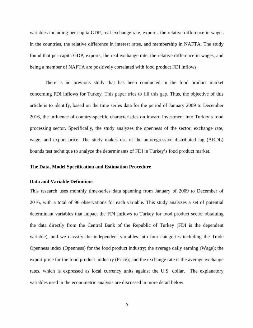
There is no previous study that has been conducted in the food product market
concerning FDI inflows for Turkey. This paper tries to fill this gap. Thus, the objective of this
article is to identify, based on the time series data for the period of January 2009 to December
2016, the influence of country-specific characteristics on inward investment into Turkey’s food
processing sector. Specifically, the study analyzes the openness of the sector, exchange rate,
wage, and export price. The study makes use of the autoregressive distributed lag (ARDL)
bounds test technique to analyze the determinants of FDI in Turkey’s food product market.
The Data, Model Specification and Estimation Procedure
Data and Variable Definitions
This research uses monthly time-series data spanning from January of 2009 to December of
2016, with a total of 96 observations for each variable. This study analyzes a set of potential
determinant variables that impact the FDI inflows to Turkey for food product sector obtaining
the data directly from the Central Bank of the Republic of Turkey (FDI is the dependent
variable), and we classify the independent variables into four categories including the Trade
Openness index (Openness) for the food product industry; the average daily earning (Wage); the
export price for the food product industry (Price); and the exchange rate is the average exchange
rates, which is expressed as local currency units against the U.S. dollar. The explanatory
variables used in the econometric analysis are discussed in more detail below.

10
Trade Openness
Trade openness is used to measure a country’s degree of openness. In the existing literature, a
large of number of empirical studies have been documented to test the link between trade
openness and FDI (Jordaan, 2004; Demirhan, 2008; Sridharan et al., 2010; Blonigen and Piger,
2011; Grubaugh S. G., 2013; Guris and Gozgur, 2015). Empirical findings of the studies claim
that there is mixed evidence concerning the effect of openness on FDI flows and that it depends
on the type of investment. In this study, we use the degree of openness index1 that is computed as
the sum of the monthly seasonal and calendar adjusted export index and import index divided by
the monthly seasonal and calendar adjusted industrial production index for the food processing
industry. Foreign trade indices monitor an overall measure of value and volume changes of
imported and exported goods. The data for trade openness for the food processing industry are
obtained directly from the Turkish Statistical Institute (TurkStat). The variable is used in its
natural log form and is expressed in US dollars.
Hypothesis 1: Higher levels of trade openness in a sector, the greater the levels of FDI
that sector should attract.
Export Price
The impact of export price depends on the level of the country’s development. Makki et. al.
(2003) show that the export price reduces the level of FDI inflows to developed countries, but
increases in the developing countries s (Makki et. al., 2003). In this study, we use consumer price
index for food processing sector in order to test the relationship between export price and FDI
inflows. The expected sign of the export price on FDI flows for the food processing industry is
1 The Openness Index is an economic metric calculated as the ratio of country's total trade, the sum of exports plus imports, to the country’s gross domestic product ((X+M)/GDP) (Wikipedia).

11
positive and the data for export price, indicated by the unit value of imports, for the food
processing industry are obtained directly from the Turkish Statistical Institute (TurkStat). The
variable is used in its natural log form and is expressed in US dollars.
Hypothesis 2: A higher price in a sector increases the level of inward FDI to the host
country, holding everything else constant.
Wage Rate
Wage rate influences the level of FDI inflows into the host country. Several researchers
determined various mechanisms through which the inward FDI may have different effect on
wages in the recipient countries. The expected sign of the wage rate on FDI flows for the food
processing industry is negative and the purpose of the MNEs is to cut their production costs by
reducing labor costs as much as possible. Thus, wage rate is the one of the important factor that
affects foreign investors’ decisions whether to invest abroad or not, this is because they choose
their investment locations based on labor costs (Makki et. al., 2003). The data for wages for the
food processing industry are obtained directly from the Turkish Social Security Institute. The
variable is used in its natural log form and is expressed in US dollars.
Hypothesis 3: A high wage in a sector decreases the level of inward FDI, other things
being constant.
Exchange Rate
A number of studies have examined the relationship between the exchange rates and FDI flows.
These studies all amounted to divergent empirical findings. In existing literature, some studies
suggest that exchange rate affects the inflows of FDI to host countries either positive or negative

12
way. Therefore, there is no clear statement as to how exchange rates affect FDI. For example,
Barrel and Pain (1998) found that a depreciation in the host countries’ currencies increased FDI
flows whereas Waldkirch (2003) concluded that an appreciation of host currency increases FDI
flows into Mexico. However, Amuedo-Dorantes and Pozo (2001) reported that no statistically
significant relationship between the level of the exchange rate and inward FDI flows into the
United States. The data for exchange rate is obtained directly from the Central Bank of the
Republic of Turkey. The variable is used in its natural log form and is expressed in US dollars.
Model Specification and Estimation Procedure
To analyze the determinants of FDI, we use the following reduced form:
FDIt = f(Pricet, Waget, ExchangeRatet, Opennesst, u) (1)
where 𝐹𝐹𝐺𝐺𝐹𝐹𝑜𝑜 is the inflows of foreign direct investment for food, beverage, and tobacco
product in the host country, 𝑃𝑃𝑃𝑃𝑃𝑃𝑃𝑃𝑃𝑃𝑜𝑜 is export prices, indicated by the unit value of
imports, 𝑊𝑊𝑊𝑊𝑊𝑊𝑃𝑃𝑜𝑜 is the average daily earning, 𝑂𝑂𝑂𝑂𝑃𝑃𝑂𝑂𝑂𝑂𝑃𝑃𝑂𝑂𝑂𝑂𝑜𝑜 is the openness of the
economy, 𝐸𝐸𝐸𝐸𝑃𝑃ℎ𝑊𝑊𝑂𝑂𝑊𝑊𝑃𝑃𝑅𝑅𝑊𝑊𝑅𝑅𝑃𝑃𝑜𝑜 is the average exchange rates expressed in local currency
units against the U.S. dollar and 𝑢𝑢 is the error term.
For computational purposes, as stated above, all variables are expressed in
logarithmic values in order to eliminate or reduce the effect of any heteroscedasticity
problem for economic time series data. Thus, the regression equation used for this
econometric analysis is:
ln(𝐹𝐹𝐺𝐺𝐹𝐹)t = 𝛼𝛼0 + 𝛼𝛼1 ln(𝑃𝑃𝑃𝑃𝑃𝑃𝑃𝑃𝑃𝑃)𝑜𝑜 + 𝛼𝛼2 ln(𝑊𝑊𝑊𝑊𝑊𝑊𝑃𝑃)𝑜𝑜 + 𝛼𝛼3ln(ExchangeRatet)𝑜𝑜 + 𝛼𝛼4 ln(𝑂𝑂𝑂𝑂𝑃𝑃𝑂𝑂𝑂𝑂𝑃𝑃𝑂𝑂𝑂𝑂)𝑜𝑜 + 𝑢𝑢𝑜𝑜 (2)

13
where the variables are as stated before and where the parameters to be estimated are 𝛼𝛼1,𝛼𝛼2,𝛼𝛼3,
𝛼𝛼4, and 𝛼𝛼5 stand for the long-run elasticities of FDI with respect to Price, Wage, Exchange rate,
and Openness, respectively. The stochastic error term is denoted by 𝑢𝑢𝑜𝑜 that satisfies the normal
requirements, and t represents monthly time period.
In terms of methodology, this study makes use of the Autoregressive Distributed Lag
(ARDL) model (or the bounds test approach) which was originally proposed by Pesaran and Shin
(1997) and gained importance by Pesaran et al. (2001). If the order of integration of the
underlying variables is purely I (0), purely I (1), or a mixture of both, then the ARDL approach is
more appropriate model than other time series methods.
An ARDL representation of equation (2) is formulated as follows:
∆ ln(𝐹𝐹𝐺𝐺𝐹𝐹)𝑜𝑜 = 𝛽𝛽0 + 𝛼𝛼1𝑖𝑖
𝑜𝑜
𝑖𝑖=1
∆𝐹𝐹𝑂𝑂(𝐹𝐹𝐺𝐺𝐹𝐹)(𝑜𝑜−𝑖𝑖) + 𝛼𝛼2𝑖𝑖
𝑜𝑜
𝑖𝑖=0
∆𝐹𝐹𝑂𝑂(𝑃𝑃𝑃𝑃𝑃𝑃𝑃𝑃𝑃𝑃)(𝑜𝑜−𝑖𝑖) + 𝛼𝛼3𝑖𝑖
𝑜𝑜
𝑖𝑖=0
∆𝐹𝐹𝑂𝑂(𝑊𝑊𝑊𝑊𝑊𝑊𝑃𝑃)(𝑜𝑜−𝑖𝑖)
+ 𝛼𝛼4𝑖𝑖
𝑜𝑜
𝑖𝑖=0
∆𝐹𝐹𝑂𝑂(ExchangeRate)(𝑜𝑜−𝑖𝑖) + 𝛼𝛼5𝑖𝑖
𝑜𝑜
𝑖𝑖=0
∆𝐹𝐹𝑂𝑂(𝑂𝑂𝑂𝑂𝑃𝑃𝑂𝑂𝑂𝑂𝑃𝑃𝑂𝑂𝑂𝑂)(𝑜𝑜−𝑖𝑖) + 𝜃𝜃1𝑙𝑙𝑂𝑂(𝐹𝐹𝐺𝐺𝐹𝐹)𝑜𝑜−1
+ 𝜃𝜃2𝑙𝑙𝑂𝑂(𝑃𝑃𝑃𝑃𝑃𝑃𝑃𝑃𝑃𝑃)𝑜𝑜−1 + 𝜃𝜃3𝑙𝑙𝑂𝑂(𝑊𝑊𝑊𝑊𝑊𝑊𝑃𝑃)𝑜𝑜−1 + 𝜃𝜃4𝑙𝑙𝑂𝑂(ExchangeRate)𝑜𝑜−1 + 𝜃𝜃5 𝑙𝑙𝑂𝑂(𝑂𝑂𝑂𝑂𝑃𝑃𝑂𝑂𝑂𝑂𝑃𝑃𝑂𝑂𝑂𝑂)𝑜𝑜−1 + 𝑣𝑣𝑜𝑜
where all variables are as previously defined, ∆ denotes the first difference operator; m’s are the
optimal lag length; the terms with summation signs represent the error correction dynamics
(short run multipliers of the model), i.e. 𝛼𝛼1𝑖𝑖,𝛼𝛼2𝑖𝑖,𝛼𝛼3𝑖𝑖,𝛼𝛼4𝑖𝑖 , and 𝛼𝛼5𝑖𝑖, and the second part of the
equation (the terms with 𝜃𝜃′𝑂𝑂) represents the long-run multipliers of the model; 𝛽𝛽0 is the drift
component, and 𝑣𝑣𝑜𝑜 is the white noise errors.
After estimating equation (2) using OLS technique, the null hypothesis of the non-
existence of the long-run relationship amongst the variables is conducted, i.e. 𝐻𝐻0: 𝜃𝜃1 = 𝜃𝜃2 =
𝜃𝜃3 = 𝜃𝜃4 = 𝜃𝜃5 = 0 against the alternative hypothesis 𝐻𝐻0: 𝜃𝜃1 ≠ 𝜃𝜃2 ≠ 𝜃𝜃3 ≠ 𝜃𝜃4 ≠ 𝜃𝜃5 ≠ 0,. The
(3)

14
joint F-statistic or Wald statistic can be used for testing the significance of the coefficients on the
lagged levels of the explanatory variables in the conditional-error correction form of the ARDL
model. Four sets of appropriate asymptotic critical value bounds for the F-statistics, such as 1
percent, 2.5 percent, 5 percent, and 10 percent, for each level of significance are tabulated by
Pesaran and Pesaran (2009) and the calculated F-statistic value is compared with the critical
values. If the computed F-value is above the upper bound critical level (for (I(1)), the null
hypothesis is rejected which implies there is a long-run co-integration association among the
time series. Contrarily, if the computed F-value is smaller than the lower bound critical value
(for (I(0)), the null hypothesis cannot be rejected which concludes that there is no long-run
association among the time series. Finally, if the F-value lies within lower and upper critical
bounds, however, the result is inconclusive.
Once a long-run relationship has been established, the second step is to estimate equation
(3) using the appropriate lag length based on the Akaike’s Information Criterion (AIC). The
third and final stage is to estimate the short-run dynamics by constructing a one-period lagged
error correction version of the ARDL model, which is associated with the long-run coefficients.
This is specified as follows:
∆ln(𝐹𝐹𝐺𝐺𝐹𝐹)𝑜𝑜 = 𝛽𝛽0 + ∑ 𝛼𝛼1𝑝𝑝𝑖𝑖=1 ∆𝐹𝐹𝑂𝑂(𝐹𝐹𝐺𝐺𝐹𝐹)(𝑜𝑜−𝑖𝑖) + ∑ 𝛼𝛼2∆
𝑞𝑞1𝑖𝑖=0 𝐹𝐹𝑂𝑂(𝑃𝑃𝑃𝑃𝑃𝑃𝑃𝑃𝑃𝑃)(𝑜𝑜−𝑖𝑖) + ∑ 𝛼𝛼3
𝑞𝑞2𝑖𝑖=0 ∆𝐹𝐹𝑂𝑂(𝑊𝑊𝑊𝑊𝑊𝑊𝑃𝑃)(𝑜𝑜−𝑖𝑖) +
∑ 𝛼𝛼4𝑞𝑞3𝑖𝑖=0 ∆𝐹𝐹𝑂𝑂(ExchangeRate)(𝑜𝑜−𝑖𝑖) + ∑ 𝛼𝛼5
𝑞𝑞4𝑖𝑖=0 ∆𝐹𝐹𝑂𝑂(𝑂𝑂𝑂𝑂𝑃𝑃𝑂𝑂𝑂𝑂𝑃𝑃𝑂𝑂)(𝑜𝑜−𝑖𝑖) +𝜓𝜓𝐸𝐸𝐶𝐶𝐶𝐶𝑅𝑅−1 + 𝜀𝜀𝑅𝑅
where 𝛼𝛼1𝑖𝑖,𝛼𝛼2𝑖𝑖,𝛼𝛼3𝑖𝑖,𝛼𝛼4𝑖𝑖 and 𝛼𝛼5𝑖𝑖 denote the short-run dynamic coefficients of the model’s
convergence to equilibrium, 𝜓𝜓 is the speed of adjustment for the explained variable towards
long-run equilibrium and ECT is the error correction. The error correction term (ECT) is defined
as: 𝐸𝐸𝐶𝐶𝐶𝐶 = 𝑙𝑙𝑂𝑂𝐹𝐹𝐺𝐺𝐹𝐹𝑜𝑜 − (𝜑𝜑1𝑙𝑙𝑂𝑂𝑃𝑃𝑃𝑃𝑃𝑃𝑃𝑃𝑃𝑃𝑜𝑜 + 𝜑𝜑2𝑙𝑙𝑂𝑂𝑊𝑊𝑊𝑊𝑊𝑊𝑃𝑃 + 𝜑𝜑3𝑙𝑙𝑂𝑂𝐸𝐸𝐸𝐸𝑃𝑃ℎ𝑊𝑊𝑂𝑂𝑊𝑊𝑃𝑃𝑅𝑅𝑊𝑊𝑅𝑅𝑃𝑃𝑜𝑜 + 𝜑𝜑4𝑙𝑙𝑂𝑂𝑂𝑂𝑂𝑂𝑃𝑃𝑂𝑂𝑂𝑂𝑃𝑃𝑂𝑂𝑂𝑂)
(4)

15
and the coefficient of ECT (𝜓𝜓) is expected to be less than zero and statistically significant in
order to imply co-integration relationship.
Empirical Analysis and Results
This section discusses the findings of various stages of analysis including the descriptive
statistics, unit root results for stationarity test, ARDL bounds test for co-integration, the estimates
of long-run coefficients, and the diagnostic tests of the model.
Descriptive Statistics
Monthly data over the period of January, 2009, to December, 2016 were used to estimate
equation (1). The descriptive statistics of the selected variables are reported in Table 1.2. Among
all variables, Openness is the lowest standard deviation values with 0.151 that states the ranking
of this variable in explaining variability in FDI. In addition, the monthly FDI inflow has highest
mean and standard deviation of 16.448 and 1.579 respectively in the data.
Results from Unit Root Test
A number of unit root tests have been developed to test the stationarity of the variables and the
conclusions of those stationary tests may differ from each other (Nieh and Wang, 2005). This
paper performs two different unit root tests, i.e., Augmented Dickey and Fuller (ADF, 1981) and
Philips and Perron (PP, 1988) to check the order of integration of the variables under
consideration by examining the Akaike information criteria (AIC) with maximum lag lengths.
All the tests mentioned above are testing the null hypothesis of stationary data. Table 1.3.
reports the results of the two different stationary tests.
The variables lnFDI and lnOpenness are stationary in level form I(0), whereas other
variables, i.e., lnExchangeRate, lnPrice and lnWage are non-stationary in their level form. After

16
differencing the data, the unit root test reveals that the series for lnExchangeRate, lnPrice and
lnWage became stationary and integrated of order I(1). Therefore, the findings obtained from the
tests clearly indicate that the series are integrated with a mixture of I(0) and I(1) which support
the use of the ARDL co-integration technique to determine the long-run relationships between
variables.
Results from ARDL Bound Tests for Co-integration
The computed F-statistics and Wald-statistics for the model are 13.578 and 708.337 respectively.
Through the results, it is evident that both the statistics are greater than the upper critical bound
values for 1 percent level of significance (4.37) which push to accept the hypothesis of co-
integration among foreign direct investment, exchange rate, trade openness, labor force, and
export price in the model. The findings of the F-statistic and Wald for the ARDL model is
reported in Table 1.4 and Table 1.5.
After confirming the co-integration association among variables, the next step is to select
the long-run ARDL model. Akaike’s Information Criterion (AIC), Schwarz Information
Criterion (SIC), and Hannan-Quinn Information Criterion (HQC) are used in the determination
of optimal lag length for the ARDL model by testing the lowest number of lags and concludes
that the ARDL model satisfies the condition of the tests of serial autocorrelation,
heteroscedasticity, and normality at the same time. Pesaran and Pesaran (1997) suggest to choose
12 lags as the optimal lag length given the fact that it uses monthly data covering the period of
January, 2009, to December, 2016. Given the maximum number of lags length (12) and the
number of variables employed (5), we selected the lag 11, which corresponds to the ARDL

17
(1,0,0,8,2)2P for long-run model after various specification trials. The results of the appropriate
ARDL model based on AIC, SIC, and HQC are reported in Table 1.6 with diagnostic tests’
statistics of the model.
Discussion of Long-run Results
The long-run coefficients of the variables under investigations are reported in Table 1.7. The test
statistics in Table 1.7 suggest that all independent variables reported in the model were
statistically significant at the different significance levels and the sign of the variables are
consistent with theoretical predictions in determining a long-run relationship in Turkey within
the study period.
The coefficient of ExchangeRate is significantly not different from zero at any significant
levels with a coefficient value of -0.404 and a p-value of 0.174. The variability of ExchangeRate
in Turkey for the food product sectors is insignificant which is not affecting the variability of the
inflow of FDI. No firm conclusion can be drawn.
The impact of the degree of openness, Openness, which is measured as trade index is
positive and significant at the 5% level. From the result, a change in trade openness index by 1
percent leads to an increase in FDI flows for the food product industry by 2.20 %, all things
being considered equal. This result suggests that openness is an important factor in explaining
FDI inflows for the food product sectors in Turkey which supports evidence of openness being a
significant determinant of FDI found by earlier studies such as Jordaan (2004), Demirhan (2008),
Sridharan et al. (2010); Blonigen and Piger (2011), Guris and Gozgur (2015). In addition,
2 𝑨𝑨𝑨𝑨𝑨𝑨𝑨𝑨 (𝟏𝟏,𝟎𝟎,𝟎𝟎,𝟖𝟖,𝟐𝟐) indicates that 1 lags for FDI, 8 lags for Exchange Rate, 0 lags for both Export Price and Openness, and 2 lags for Wage.

18
foreign investors place much importance on the degree of openness of the Turkish economy
while determining the location of economic activities.
Considering the impact of the export price to FDI, the statistic of price of export is
significantly different from zero at 1% significant level with a coefficient value of 3.57 and a p-
value of 0.066. This result suggests that holding everything else constant, a change in export
price index by one-percentage point causes 3.57 percentage-point increase the level of FDI flows
for the food product industry in Turkey. This result is consistent with Makki et.al. (2003).
Lastly, the coefficient of Wage, in the long run, was found to have a negative sign in the
line with expectations of this study and statistically significant at 1 %. From the result, one-
percent increase in wage rate is associated with a 2.74 % decrease on inward FDI for the food
product sectors in Turkey.
On the other hand, the coefficient on the lagged error correction term is highly significant
at the 1 percent level with the expected sign which suggests that the error correction model is
well fitted. More precisely, the coefficient of ECT is estimated to -0.92 (0.000) which indicates
that approximately 92 percent of the disequilibrium in FDI from the previous period’s shock will
be converged back to the long-run equilibrium in the current period.
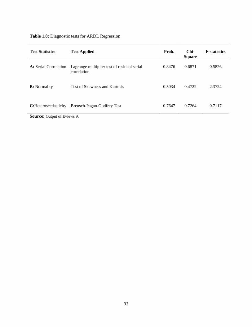
Diagnostic Tests
In this section, several diagnostic tests were performed to verify the stability of the model. The
results of these tests are given in Table 1.8. In serial correlation, the probability of the F-stat
value for the Breusch-Pagan Lagrange Multiplier (BPG LM) test is 0.847 which is greater than
the 5 percent significant levels and it implies that there is no serial correlation in the long run
relationship. Further, the probability of the data is higher than the 5% significant level, which

19
shows that the data used for the model is normally distributed. Finally, we use BPG test to check
whether the model suffers from a heteroscedasticity problem or not, and we conclude that there
is no heteroscedasticity problem in the model.
In order to determine the goodness of fit of the ARDL model, the stability tests proposed
by Borensztein et al. (1998) and suggested by Pesaran and Pesaran (1997), Pesaran and Shin
(1999), and Mohsen et al. (2002) have been employed to examine the stability of short-run and
long-run coefficients. For test, the cumulative sum (CUSUM) and the cumulative sum of squares
(CUSUMQ) stability tests have been performed to assess the parameter constancy on the basis of
the AIC-based error correction models. The results of Figures 1 and 2 clearly confirm that the
parameters are stable over the sample period since the plot of the CUSUM and CUSUMQ
statistics stay within the 5% level of significance. Thus, the null hypothesis of all coefficients
under estimation is steady and cannot be rejected.
Concluding Remarks
In the literature, few empirical studies investigate the determinants of FDI inflows for the food
product industry, and none exists for Turkey. Therefore, this paper attempts to fill in this gap.
Based on review of previous studies, we have identified four important determinants that
generally influence FDI. They are, trade openness, export price, and wage rate. This study has
tested the long-run cointegration relationship between the variables under study by using Error
Correction Model (ECM) based on the ARDL bound testing approach during the period of
January, 2009, to December, 2016. The significance of both the F-statistic and Wald statistic of
the ARDL model confirms the presence of a long-run relationship among variables.

20
It is also found that the variable trade openness, which is measured as trade index, has a positive
relationship with FDI in the long run. We conclude that trade openness is a crucial factor in
promoting Turkey’s food product FDI. As argued earlier, on the basis of this result, countries
with an efficient investment environment and greater trade liberalization policies promote FDI
inflows into the host country.
The export price has a positive effect on Turkish food processing industry. This finding means
that when export prices increase, MNEs make an effort to invest more into the host country in
order to raise their profits. This result is further supported by Makki et.al. (2003).
The empirical results show that the variable wage rate has a negative effect on FDI
inflows for food processing industry in Turkey. This conclusion implies that the higher wage
rate in food processing sector reduces the level of FDI inflows to Turkey.
Moreover, other results show that the error-correction coefficient, which determines the
speed of adjustment, had the expected negative sign and is significant. The finding suggests that
deviations from long-term disequilibrium in FDI inflows are corrected by approximately 81
percent in each of the following period. In addition to those results, the model passes all of the
diagnostics and stability tests.
Based on the conclusions above, these empirical findings have important key
recommendations to policy makers. Since 2002, based on the 2023 vision that is the 100th
anniversary of the Republic of Turkey, Turkish government has introduced four different
incentive schemes in 2003, 2006, 2009, and 2012 in order to provide economic and financial
stability, to expand the local economy, and to regulate its investment climate for more FDI
inflows into the country. Yet, none of these incentive schemes did not help Turkey’s food

21
processing sector as a desirable level. Thus, the Turkish government should prepare a specific
program to protect the foreign investors in this industry. Further, the Turkish government also
needs to formulate and implement prudent policies in order to enhance Turkey’s dynamics such
infrastructure, human capital quality, financial sector intermediation, labor market performance.

22
References
Amuedo-Dorantes, C. and Pozo, S. (2001). Exchange-Rate Uncertainty and Economic
Performance. Review of Development Economics 5 (3): 355-446.
Atalaysun, M., (2012). “Retail Foods Report” USDA GAIN Report.
Athukorala P., and Sen, K. (1998). ‘Processed Food Exports from Developing Countries:
Patterns and Determinants’, Food Policy 23(1):41–54.
Barrell, R. and Pain, N. (1998). Real exchange rate, agglomerations, and irreversibilities:
macroeconomic policy and FDI in EMU. Oxford Review of Economic Policy 14(3):
152-167
Berkum, S.V., (1999). “Patterns of Intra-Industry Trade and Foreign Direct Investment in Agro-
Food Products: implications for East-West Integration.” Agricultural Economics
Research institute (LEI), In MOCT-MOST, No.3, pp.225-271.
Blonigen, B. A., & Piger, J. (2011). “Determinants of foreign direct investment” National Bureau
of Economic Research, Inc, NBER Working Papers: No.16704
Bolling, C. and A.Sumwaru (2001), “U.S. food companies access foreign markets through direct
investment.” Food Review 24 (September-December ): 23-28
Borensztein, E., De Gregorio J., and J.W.Lee. (1998). “How does FDI affect economic growth.”
Journal of International Economics, Vol.45, No.1, pp.115-135.
Business Reporter, (2013). “A vibrant nation where East meets West,” Invest in Turkey,
Comert, H. and S. Colak, (2014) “The Impacts of Global Crisis on the Turkish Economy and
Policy Responses” ERC Working Papers in Economics 14/17, pp.1-28.
Demirhan, E., & Masca, M. (2008). “Determinants of foreign direct investment flows to
developing countries: a cross-sectional analysis.” Prague Economic Papers, 4, pp. 356 -
369.
Ernst & Young’s attractive survey, (2013). “The shift, the growth and the promise” Growing
Beyond.
FAO (2015). ‘The State of Food Insecurity in the World 2015. Meeting the 2015 international
hunger targets: taking stock of uneven progress’, Food and Agriculture Organization of
the United Nations. Rome, Italy.

23
Gerlach, A. C., & Liu, P. (2010). ‘Resource-seeking Foreign Direct Investment in African
Agriculture A review of country case studies’, FAO Commodity and Trade Policy
Research Working Paper No. 31.
Gibbon, P., and Ponte, S. (2005). Trading Down: Africa, Value Chains and the Global Economy.
Temple University Press.
Gopinath, M., D. Pick, and U. Vasavada (1999). “The Economics of Foreign Direct Investment
and Trade with an Application to the U.S. Food Processing Industry.” American Journal
of Agricultural Economics, 81: 442-52.
Grubaugh, S. G. (2013). “Determinants of Inward Foreign Direct Investment: A Dynamic Panel
Study.” International Journal of Economics & Finance, Vol.5, No.12.
Guris, S. and K. Gozgur, (2015). “Trade Openness and FDI Inflows in Turkey.” Applied
Econometrics and International Development, Vol. 15, No. 2, pp. 53-62.
Hallam, D. (2009). Foreign Investment in Developing Country Agriculture- Issues, Policy
Implications and International Response.
Jordaan, J.C. (2005). “Foreign Direct Investment and Neighbouring Influences” Unpublished
doctoral Thesis, University of Pretoria.
Josling, T. and S. Tangermann, (1996). “The Agricultural and Food Sectors” BRIE Working
Paper, No.103.
Makki, S.S., Somwaru, A. and Bolling, C. (2003), “Determinants of US foreign direct
investments in food processing industry: evidence from developed and developing
countries”, paper prepared for presentation at the American Agricultural Economics
Association Annual Meeting, Montreal, July 27-30.
Mattson, J., and W. Koo (2002) “Canadian Exports of Wheat and Barley to the United States and
Impacts on U.S. Domestic Prices,” ed. W. Koo, and W. Wilson. Hauppauge, NY, Nova
Science Publishers, Inc., pp. 73-92.
Nieh, Chien-Chung and Wang, Yu-shan (2005). ARDL Approach to the Exchange Rate
Overshooting in Taiwan. Review of Quantitative Finance and Accounting, 25: 55-71.
Parajuli, S. (2012). “Examining the relationship between the exchange rate, foreign direct
investment and trade,” Unpublished doctoral thesis, Louisiana State University.
Pesaran, M. H., and B. Pesaran. (1999). “Working with Microfit 4.0: interactive econometrics
analysis.” Oxford University Press, New York.

24
Pesaran, M. H., and B. Pesaran. (2009). “Time Series Econometrics using Microfit 5.0.” Oxford
University Press, New York.
Pesaran, M. H., Yongcheol S., and S. Richard. (2001). “Bound Testing Approaches to the
Analysis of Level Relationships.” Journal of Applied Econometrics, Vol.16, No.3, pp.
289- 326.
Sanderatne, N. (2011). Columns - The Sunday Times Economic Analysis. Retrieved 15 May, 2017
from http://www.sundaytimes.lk/110529/Columns/eco.html
Slimane, M. B., Huchet-Bourdon, M., & Zitouna, H. (2015). ‘The role of sectoral FDI in
promoting agricultural production and improving food security’, Economie
Internationale, pp.34.
Smith, F., & Häberli, C. (2012). ‘Food Security, Foreign Direct Investment and Multilevel
Governance in Weak States’, Society of International Economic Law (SIEL), 3rd Biennial
Global Conference.
_______, (2009). Turkish Social Security Institute.
_______, (2017). Turkish Social Security Institute.
_______, (2017). Turkish Statistical Institute.
_______, (2017). The Central Bank of the Republic of Turkey (CBRT).
UNCTAD, (2005). The Least Developed Countries Report 2006. New York.
Waldkirch, A. (2003). The 'new regionalism' and foreign direct investment: the case of Mexico.
Journal of International Trade and Economic Development 12(2): 151-184
Walkenhorst, P. (2001) “Determinants of foreign direct investment in the food industry: The case
of Poland” Agribusiness, Vol.17, No.3, pp.383-395.
Wilson, N. (2006) “Linkages amongst Foreign Direct Investment, Tarde and Trade Policy: An
Economic analysis with Applications to the food Sector” Presented at the American
Agricultural Economics Association Annual Meeting, Long Beach, California.
Wilson, N. and J. Cacho (2007) “Linkage Between foreign Direct Investment, Trade and Trade
Policy.” OECD Publishing.
Xun, L (2006). “The Determinants of U.S. Outgoing FDI in the Food-Processing Sector” UMI
Microform.
25
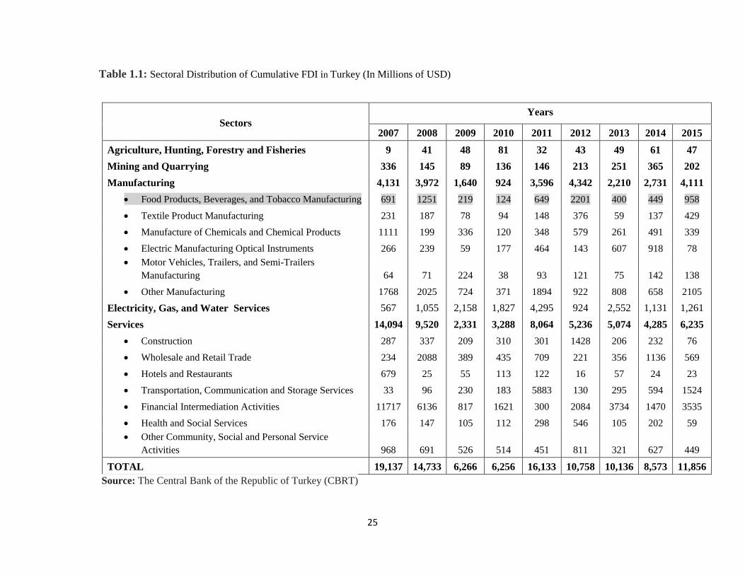
Table 1.1: Sectoral Distribution of Cumulative FDI in Turkey (In Millions of USD)
Sectors
Years
2007 2008 2009 2010 2011 2012 2013 2014 2015 Agriculture, Hunting, Forestry and Fisheries 9 41 48 81 32 43 49 61 47 Mining and Quarrying 336 145 89 136 146 213 251 365 202 Manufacturing 4,131 3,972 1,640 924 3,596 4,342 2,210 2,731 4,111
• Food Products, Beverages, and Tobacco Manufacturing 691 1251 219 124 649 2201 400 449 958
• Textile Product Manufacturing 231 187 78 94 148 376 59 137 429
• Manufacture of Chemicals and Chemical Products 1111 199 336 120 348 579 261 491 339
• Electric Manufacturing Optical Instruments 266 239 59 177 464 143 607 918 78 • Motor Vehicles, Trailers, and Semi-Trailers
Manufacturing 64 71 224 38 93 121 75 142 138
• Other Manufacturing 1768 2025 724 371 1894 922 808 658 2105
Electricity, Gas, and Water Services 567 1,055 2,158 1,827 4,295 924 2,552 1,131 1,261 Services 14,094 9,520 2,331 3,288 8,064 5,236 5,074 4,285 6,235
• Construction 287 337 209 310 301 1428 206 232 76
• Wholesale and Retail Trade 234 2088 389 435 709 221 356 1136 569
• Hotels and Restaurants 679 25 55 113 122 16 57 24 23
• Transportation, Communication and Storage Services 33 96 230 183 5883 130 295 594 1524
• Financial Intermediation Activities 11717 6136 817 1621 300 2084 3734 1470 3535
• Health and Social Services 176 147 105 112 298 546 105 202 59 • Other Community, Social and Personal Service
Activities 968 691 526 514 451 811 321 627 449
TOTAL 19,137 14,733 6,266 6,256 16,133 10,758 10,136 8,573 11,856 Source: The Central Bank of the Republic of Turkey (CBRT)

26
Table 1.2: Definitions and descriptive statistics of the variables used in the empirical analysis
Variable Definition Descriptive Statistics
Obs. Mean S.D. Median Min. Max.
FDI
Foreign direct investment inflows of for food product industry (natural logarithm)
96
16.448
1.579
16.523
13.815
21.375
Openness
Trade Openness Index for food product industry calculated with the 2005 base year (natural logarithm)
96
0.855
0.151
0.815
0.547
1.239
Wage
Average monthly wage for food product industry (natural logarithm)
96
4.413
0.250
4.410
3.929
4.917
Export Price
Export price, indicated by the unit value of imports, for the food processing industry (natural logarithm)
96
5.654
0.244
5.684
5.180
6.099
Exchange Rate
Exchange rate is the average exchange rates expressed in local currency units against the U.S. dollar (natural logarithm)
96
0.682
0.247
0.594
0.349
1.249
Source: Author’s calculation using Eviews 9.

27
Table 1.3: The results of various unit root tests on the log values of the variables based on SIC
ADF
PP
Variable
𝛕𝛕𝐜𝐜
𝛕𝛕𝐜𝐜+𝐭𝐭
𝛕𝛕𝐜𝐜
𝛕𝛕𝐜𝐜+𝐭𝐭
FDI
-8.8056*** [0] (0.0000)
-9.0128*** [0] (0.0000)
-8.8520*** [3] (0.0000)
-43.5444*** [26] (0.0001)
Exchange Rate
1.6862[0] (0.9996)
-2.5838 [1] (0.2886)
1.4189 [1] (0.9990)
-1.8976 [2] (0.6480)
Openness
-3.9056*** [0] (0.0029)
-3.8418*** [0] (0.0185)
-3.9056*** [0] (0.0029)
-3.8418*** [0] (0.0185)
Export Price
-0.6844 [0] (0.8449)
-3.9788** [1] (0.0126)
-0.6749 [4] (0.8472)
-3.4435 [0] (0.0518)
Wage
1.6039 [11] (0.9994)
-6.7953*** [7] (0.0000)
-0.2290 [7] (0.9299)
-9.3714*** [6] (0.0000)
FDI
na
na
na
na
Exchange Rate
-7.1640*** [0] (0.0000)
-7.6173*** [0] (0.0000)
-7.1640*** [0] (0.0000)
-7.5809*** [2] (0.0000)
Openness
na
-11.4687*** [0] (0.0000)
na
-12.7621*** [9] (0.0000)
Export Price
-8.7073*** [0] (0.0000)
na
-8.6321*** [5] (0.0000)
-8.5715*** [5] (0.0000)
Wage
-6.7953*** [7] (0.0000)
na
-25.0077*** [5] (0.0001)
na
1% level*** -3.5104 -3.5073 -3.5006 -4.0575 5% level** -2.8925 -2.8951 -2.8922 -3.4578 10% level* -2.5833 -2.5847 -2.5831 -3.1548
Notes: All variables are in logs in the series. Asterisks (***) and (**) show values are significant at 1% and 5% level with MacKinnon (1996), respectively. The figures within the [.] for the ADF are the appropriate lag lengths selected by SIC (Schwarz Info Criterion), whereas the figures within the parentheses for the PP is the optimal bandwidths decided by the Barnett kernel of Newey and West (1994). denotes the first difference of the variable. Results obtained from Eviews 9.

28
Table 1.4: ARDL Bounds Test for Co-integration
Variables
F-Statistics
Inference
F(FDI / Price, Exchange Rate, Openness, Wage)
13.578***
Co-integration
Significance Value Lower Bound Upper Bound
1% 2.20 3.09
2.5% 2.56 3.49
5% 2.88 3.87
10% 3.29 4.37
Notes: *** Statistical level at 1% level; ** Statistical level at 5% level; and * Statistical level at 10% level. The lag length k=11 was selected based on the Akaike info criterion (AIC), Schwarz Info criterion (SCi) and Hannan-Quinn criterion (HQC). Results obtained from Eviews 9.

29
Table 1.5: ARDL Bounds Test for Co-integration
Wald Test: Long-run Relationship
Test Statistics F-Statistics Chi-Square
Value
708.337*** 11333.40
DF
(16,72) 16
Probability
0.0000
0.0000
Null Hypothesis
C(1)=C(2)=C(3)=C(4)=C(5)=C(6)=C(7)=C(8)=C(9)=C(10)=C(11)=C(12)=C(13)=C(14)=C(15)=C(16)=0
Notes: *** Statistical level at 1% level. Results obtained from Eviews 9.

30
Table 1.6: ARDL Lag Length Order Selection Criteria based on AIC, SCI and HQC
Lag Length
Selected Model
AIC
SIC
HQC
𝑹𝑹𝟐𝟐
F-Stat
Normality (prob.)
Serial Correlation
Heteroscedasticity
Bound-test
ECT(-1)
1 (1,0,0,1,1) 3.784 3.999 3.871 0.126 1.802 0.719 0.705 0.889 13.952 -0.955
2 (1,0,0,1,2) 3.743 3.986 3.841 0.176 2.281 0.024 0.749 0.952 15.640 -0.981
3 (1,0,0,1,2) 3.743 3.986 3.841 0.176 2.281 0.724 0.028 0.952 15.640 -0.981
4 (1,0,0,1,2) 3.743 3.986 3.841 0.176 2.281 0.724 0.028 0.952 15.640 -0.981
5 (1,0,0,1,2) 3.743 3.986 3.841 0.176 2.281 0.724 0.028 0.952 15.640 -0.981
6 (1,0,0,1,2) 3.743 3.986 3.841 0.176 2.281 0.724 0.028 0.952 15.640 -0.981
7 (1,0,0,2,2) 3.749 4.020 3.858 0.188 2.173 0.715 0.934 0.887 14.165 -0.960
8 (1,0,0,2,2) 3.749 4.020 3.858 0.188 2.173 0.715 0.934 0.887 14.165 -0.960
9 (1,0,0,2,2) 3.749 4.020 3.858 0.188 2.173 0.715 0.934 0.887 14.165 -0.960
10 (1,0,0,2,2) 3.749 4.020 3.858 0.188 2.173 0.715 0.934 0.887 14.165 -0.960
11 (1,0,0,8,2) 3.736 4.006 3.837 0.392 2.988 0.503 0.220 0.726 13.578 -0.929
12 (12,12,12,11,10) 3.355 5.149 4.076 0.848 2.026 0.758 0.008 0.633 3.793 0.541
Source: Author's calculation using Eviews 9.

31
Table 1.7: Long-run coefficients of ARDL (1, 0, 0, 8, 2) model
Notes: 𝐑𝐑𝟐𝟐 = 0.392; 𝐃𝐃𝐃𝐃𝐃𝐃𝐃𝐃𝐃𝐃𝐃𝐃 −𝐖𝐖𝐖𝐖𝐭𝐭𝐖𝐖𝐖𝐖𝐃𝐃 = 2.121 ; 𝐅𝐅 − 𝐖𝐖𝐭𝐭𝐖𝐖𝐭𝐭 = 2.988 (0.000). ***, **, and * denote significant at 1%, 5%, and 10 % levels, respectively. Source: Author's calculation using Eviews 9.
Long run coefficients (Total Effect)
Variable Coefficient Std. Error Prob.
Openness 2.204∗∗ 1.825 0.041
Exchange Rate −0.404 3.216 0.174
Export Price 3.579∗ 4.383 0.066
Wage −2.744∗∗∗ 4.912 0.002
Constant 8.210∗ 14.449 0.057
ECT(-1) -0.929 0.104 0.000
32
Source: Output of Eviews 9.
Table 1.8: Diagnostic tests for ARDL Regression
Test Statistics
Test Applied
Prob.
Chi-Square
F-statistics
A: Serial Correlation
Lagrange multiplier test of residual serial correlation
0.8476
0.6871
0.5826
B: Normality
Test of Skewness and Kurtosis
0.5034
0.4722
2.3724
C:Heteroscedasticity
Breusch-Pagan-Godfrey Test
0.7647
0.7264
0.7117

33
Source: The Central Bank of the Republic of Turkey (CBRT)
Figure 1.1: FDI inflows (million $) and GDP Growth Relation in Turkey (Note: Values are averaged over the period 1980-2000)
-8%
-6%
-4%
-2%
0%
2%
4%
6%
8%
10%
12%
0
5
10
15
20
25Bi
llion
$
Year
FDI inflows and GDP Growth Relation in Turkey
FDI GDP Growth

34
-30
-20
-10
0
10
20
30
I II III IV I II III IV I II III IV I II III IV I II III IV I II III IV
2011 2012 2013 2014 2015 2016
CUSUM 5% Significance
Figure 1.2: Evaluation of the stationarity of short-term coefficients (CUSUM)

35
-0.2
0.0
0.2
0.4
0.6
0.8
1.0
1.2
I II III IV I II III IV I II III IV I II III IV I II III IV I II III IV
2011 2012 2013 2014 2015 2016
CUSUM of Squares 5% Significance
Figure 1.3: Evaluation of the stationarity of long-term coefficients (CUSUMQ)
36
Essay 2: Exchange Rate and Turkish Tourism Trade: is there a J-Curve?
Introduction
In today’s world, tourism is akin to globalization. Tourism, in this regard, is the movement of
peoples from one part of the world to another. But in this instance, this is a temporary stage and
these people usually come back to the place where they started their travel. This pursuit is
usually to become aware of different cultures, dance, music, clothes, and languages of other
places of interest.
With the world becoming what is termed a “global village,” tourism too is getting
enhanced in some ways. It could be business tourism, where one goes to another place with
regard to one’s occupation for professional reasons. One could be going for religious tourism
purposes, where a traveler is in search of enhancement of knowledge of a given religion or is on
a pilgrimage. Tourism could also be just for satisfying an inner desire to travel to unknown or
exotic destinations or for the thrill of the adventure involved in some activity. Whatever the case,
tourism has a direct effect bearing on globalization since the more we travel, the more global in
our outlook and thinking we become.
International tourist arrivals increased by about 4.4 percent in the year 2015 (WTO,
2016). About 50 million additional tourists, by this we mean overnight visitors, went to
international places in comparison with the year before (WTO, 2016). Also, international tourist
arrivals to the European Union increased by four percent in the year 2016. Translating into terms
of world tourism, this is about 40 percent of entire travel (UNWTO, 2017). As far as Turkey is

37
concerned, the number of foreigners in Turkey came down by 3.96 percent in March 2017 from
1.65 million in the same month previous year (Trading Economics, 2017).
Tourism has several positive impacts. First and foremost, it is a source of employment
creation. Also, it goes a long way in enhancing a country’s image on a global platform. It helps
not just to preserve the traditions, customs and culture of any given place, but also spreads them
to the home countries of the tourists. In addition, it brings foreign exchange to the country,
thereby helping the economy.
Moreover, tourism may help to improve a locale place – with visitors coming in there
may be improvements in cleanliness, environment enhancement and other benefits. Local
industry and handicrafts boost since visitors tend to purchase items for memorabilia and gifting
purposes. However, some of the negative aspects associated with tourism are that it puts pressure
on the environment. This is more so when the number of visitors to any given place is very large
and if existing resources are already strained. Tourism, when all its related spheres are not taken
care of, can cause a natural habitat loss, increased pollution, soil erosion and other negative
outcomes
The remainder of this paper is structured as follows. The first section overviews the
profile of the Turkish tourism market. The next section summarizes the relevant literature and
highlights the main contributions of this research. The following sections briefly describe the
model, methodology, the data, and report the empirical findings. Finally, the last section reports
the main conclusions of the study.
A profile of Turkish Tourism Market
Tourism is an important element of international trade and one of the largest investment and
development industries affecting local, regional, national and global economies in the world

38
(Akay et al., 2017). It offers a large amount of economic benefits such as generating new job
opportunities, encouraging the private sector, helping to improve per capita income and standard
of living, facilitating development of basic infrastructural facilities, creating a multiplier impact
on a national economy, and reducing poverty (Saayman and Saayman, 2015). It is a noteworthy
point that tourism as a field needs a lesser scale of per capita funds. Even the technological as
well as labor related skills necessary for this sector are on the lower side. Also, tourism
encounters much less of a protectionist attitude in world economies than manufacturing does.
Thus, tourism has become an appealing arena to explore for lesser developed places and
countries looking for methods for economic development (Sharma, 2004).
Thanks to its great geographical location and natural opportunities, and its many
historical, religious, and archaeological sites, Turkey is one of the leading countries in tourism.
Since free market economy policies and government's promotion of tourism in the 1980s,
tourism has come to play a major role in the Turkish economy. The Tourism Encouragement
Law of 1982 put tourism among the “sectors of special important for development.” In addition,
the Turkish government introduces many incentives – such as exceptions from several taxes
including customs and export taxes, the transfer of public land to private tourism companies, low
interest loans to the investors through the Turkish Tourism Bank, investment allowance,
concessional tariff rates for power, water, and gas consumption - to boost the tourism sector
(Özen and Kuru, 1998; Nohutcu, 2002; Yolal, 2016). As a result of these incentive policies,
tourism experienced a remarkable success after the mid-1980s.
For the reasons stated above, the number of f international visitors coming to Turkey
increased almost thirty-five times, rising from 725 thousand in 1970 to 39.4 million in 2015.
According to World Tourism Organization report, in 2016 Turkey held 6th place in the
39
international ranking of the ‘Top10’ tourist destination assessed by the number of arrivals. In
addition, in terms of tourist revenue, in 2016 Turkey occupied 12th place in the international
tourist receipts. According to the World Travel and Tourism Council Data (2013), tourism
contributes 12.5% to Turkish gross domestic product (GDP).
It also important to note that the Turkish tourism industry, in 2016, faced difficulties such
as the downing a Russian warplane by a Turkish jet in November 2015, the terrorist attack on
Istanbul’s Ataturk airport in June 2016, and a failed military coup attempt in July 2016. The
number of tourist arrivals to Turkey amounted to 25 million, a decrease by 41% compared to
2015. In addition, according to data compiled the Republic of Turkey Ministry of Culture and
Tourism, during the first quarter of 2017, Turkey welcomed 3.8 million tourists, a 6.43%
decrease over the corresponding period of 2015.
During 2007-2016, about 50% of inbound tourists staying in Turkey came from the
European Union countries (TURKSTAT, 2017). The top twelve tourists’ origin countries are, on
average, Germany, Russia, the United Kingdom, Bulgaria, Iran, Georgia, the Netherlands,
France, USA, Ukraine, Greece, and Italy. Furthermore, the number of visitors from Germany,
Russia, the Netherlands, France, USA, Italy and Greece has significantly declined in recent
times.
Review of Related Literature
There is an old saying, “The world is a great book, of which they that never stir from home read
only a page” (St. Augustine, 354-430, AD). Indeed, travelling the world enables one to see a lot
of things and gain experience concerning different cultures. Failing to travel would make one
remain within his or her cultural setting. Therefore, one would not be updated on many issues.
40
There is a multitude of previous studies on tourism. For example, Vogt (2008) analyzes the real
income and relative elasticity of demand in tourism exports and imports. The study makes use of
data from the year 1973 to 2002. The findings show that the response of the trading partners to
the changes in real income in tourism may have an impact on tourism in the country by
increasing surpluses on the tourism balance of trade in the country. The spending of people from
these countries in the United State enables trade in tourism to improve as they bring in foreign
exchange. The rates of exchange partly determine the choice of foreign tourists coming to the
country.
In their research note, Thompson and Thompson (2010) discuss the effects of exchange
rates and the adoption of the euro in tourism revenue in Greece using a sample period of 32
years. The paper identifies that tourism is a crucial factor in the economy of the country. It earns
the country a lot of foreign exchange. The results of the study show that the rates of exchange
have an impact on tourism in Greece. A depreciation of the rates of exchange enables the country
to earn more foreign exchange in tourism. It also shows that the adoption of the euro had a
positive impact on tourism in Greece. It makes the country at par with other European countries
since they have the same currency.
Cheng et al. (2013a) analyze the impact of exchange rates on tourism in the United States
using data from 1973 to 2007. The analysis discusses the revenue earned from tourism exports
and spending on travel imports with regard to the balance of trade. The results of the study show
that currency depreciation has a positive impact on the balance of tourism trade in the country.
Notably, the depreciation of foreign exchange rates facilitates more spending among the tourists
from foreign countries. They also show that travelling outside the country for tourism is
considered a luxury. However, it is common for people to travel to the United States for tourism.

41
Cheng et al. (2013b) discuss the effects of real exchange rates and income on tourism in the
United States. The paper analyzes the revenue earned by exporting tourism and spending on
imports using the data available between the years of 1973 to 2010. The results of the study show
that depreciation has a positive impact on the revenue earned from tourism exports. However, it
does not affect import spending on tourism in the country. The paper also states that when the
exchange rates drop, tourists have more to spend, increasing foreign income from tourism.
However, local tourists have no impact since they spend local currency.
More recently, Chi (2015) examined the effects of income and exchange rates on the
exports and imports of tourism in the country. He explained the trends with an aim to help
understand the determinants of the balance of trade in the tourism sector in the United States.
The findings of the study show that appreciation of the dollar has a negative impact on the trade
balance in tourism in the country. The paper also notes that the appreciation of the dollar makes
the exchange rates unfavorable for tourists, thereby making them avoid the country as a tourist
destination.
Turning to the domestic literature, a few empirical studies have been carried out on
tourism development for Turkey. For instance, Halicioglu (2010) analyzes the demand for
tourism in Turkey with regard to international exchange rates and income. The results show that
depreciation in international exchange rates has a positive impact on the demand for tourism,
thereby leading to a positive trade balance in tourism. Favorable exchange rates enable the
tourists to spend more local currency in the country.
Kilic and Bayar (2014) discuss the relationship between the volatility of the exchange
rates and expenditure on tourism in Turkey using annual data from 1994-2013. The Johansen co-
integration test is used to get the relationship between the series. The results of the study show

42
that there is a positive relationship between the rates of exchange in the country and expenditures
on tourism. When the exchange rates depreciate, international tourists are attracted to the country
leading to an increase in foreign income, which helps improve the tourism sector. In addition,
Akay et al. (2017) analyzed the effects of income and exchange rates on tourism in Turkey by
applying Johansen’s maximum likelihood approach to measure the long-term impact of the
exchange rates and income on tourism in the country. They report that income is the most
important factor that can explain the trade balance in tourism over the long-term. In particular,
the results show that foreign income and real exchange rates affect tourism in a positive manner,
while domestic income affects tourism in a negative manner. Furthermore, they point out that
when the rates of exchange are low, foreign income for the tourists would increase, making more
people choose the destination, but domestic income has no effect on tourism since there is no
foreign exchange involved.
This paper extends the Turkish tourism literature in three ways. First, this study focuses
on the dynamic interactions among the variables by applying a multivariate VAR framework.
Second, using annual data for the period 1970-2016, this study analyzes the presence of J-curve
for the eight major Turkey tourist arrival European Union (EU) countries: Australia, Belgium,
France, Germany, Greece, Netherlands, Italy, and Portugal. Third, this study employs Vector
autoregressive Model (unrestricted) (VAR) which does not provide the short run or long run
effects of the exchange rates on tourism.
Theoretical Framework for Tourism Trade
In dealing with the tourism trade balance analysis, this paper follows similar equation chosen
from Vogt (2008), Cheng et al. (2013a, 2013b), and Chi (2015), which examines the relationship

43
between exchange rate and tourism trade balance. The linear models for Turkish exports (𝑋𝑡) and
imports (𝑀𝑡) of tourism are specified as below:
𝐸𝑋𝑡 = 𝑓 (𝑌𝑡∗, 𝐸𝑡) (1)
𝐼𝑀𝑡 = 𝑓 (𝑌𝑡, 𝐸𝑡) (2)
where 𝑋𝑡 is the export revenue, 𝑀𝑡 is the import spending, 𝑌𝑡 is Turkey's income, 𝑌𝑡∗ is foreign
income, and 𝐸𝑡 is the exchange rate of Turkish lira against foreign currencies. Equation (1) and
(2) are rewritten in a double-log functional form, and we have
𝑙𝑛 𝑋𝑡 = 𝑎0 + 𝑎1 𝑙𝑛𝑌∗ + 𝑎2 𝑙𝑛𝐸𝑡 + 𝜀𝑡 (3)
𝑙𝑛 𝑀𝑡 = 𝑏0 + 𝑏1 𝑙𝑛𝑌 + 𝑏2 𝑙𝑛𝐸𝑡 + 𝜗𝑡 (4)
In the literature, trade balance is usually measured as the difference between export revenue and
import spending. In this study, following a similar approach proposed by Bahmani-Oskoosee and
Brooks (1999), Boyd et al.(2001), Onafowora (2003) and Cheng et al. (2013a, 2013b), we
measure the trade balance as the ratio of export revenue and import spending, 𝐵 ≡ 𝑋/𝑀. After
taking natural logarithm, we specify trade balance equation as follows
ln 𝐵𝑡 = 𝑙𝑛 𝑋𝑡 − 𝑙𝑛 𝑀𝑡 (5)
Substituting Equations (3) and (4) into (5), we get
ln 𝐵𝑡 = ( 𝑎0 − 𝑏0) + 𝑎1 𝑙𝑛𝑌∗ − 𝑏1 𝑙𝑛𝑌 + (𝑎2 − 𝑏2) 𝑙𝑛𝐸𝑡 + (𝜀𝑡 − 𝜗𝑡) (6)
To understand the correlation between the tourism trade and exchange rate, one must consider
the J-Curve phenomenon. J Curve serves as an example of movement in variables that declines

44
in the beginning and then gradually increases to the new higher levels than the starting point
forming the shape of letter “J” on time series graph.
This curve is mostly found in the economic situations of the country where the currency
of the country is depreciated or devalued considering the better future perspectives for the
country. It explains the situation wherein the trade deficit of a country is high initially due to
devaluation or depreciation in the currency due to higher costs of imports and lesser. With the
passage of time, the situation of exports improves due to devaluation in the country, thereby,
giving competitive advantage to the country to trade in the world and also, imports starts
declining due to the availability of cheaper products at the domestic market compared with the
imported goods. This situation brings in positive effects in the balance of payments and the net
balance of payments becomes positive giving a “J” curve effect in the economy (Staff, 2003;
Rode, 2012)
Data and Empirical Methodology
Data
As noted in the introduction, in this study, tourist arrivals from seven member countries of EU:
Australia, Belgium, France, Germany, Greece, Italy, Netherlands, and Portugal are considered.
These countries have been selected on the basis of tourism demand for Turkey from EU. To
avoid the seasonality problem, data consists of annual observations during the period 1970 -
2016. Secondary data sources were used in the study and are collected from various sources.
Data for tourism arrivals for the period 1970-2016 are obtained from Turkish Statistical Institute
(TURKSTAT). Turkey’s income is GDP and we record income for the rest of the world as the
sum of GDP of the selected countries. The foreign exchange is measured as the price of a dollar

45
in terms of Turkish liras. All GDPs are obtained from the World Bank. All variables are
expressed in natural log form.
Figure 2.1 presents the plots of all variables in natural logs. Tourism export revenue, X,
generally shows an increasing trend since 1970, while there are some fluctuations in import
spending, M, between the years. In addition, trade balance, B, is always negative except mid-
1970s. The exchange rate, E, had three periods of Turkish lira depreciation, up to late 1970s then
during the mid-1990s, and again up to 2007s, then two periods of appreciation, from 1982 to
1985 and from 1998 to 2001. Over the period 1970-2016, Turkey’s income,𝑌, and foreign
income, 𝑌∗, fluctuates between the years.
Empirical Methodology
This study applies the method of time series econometrics, which is vector autoregressive
(VAR) estimation technique to model the exchange rate and tourism trade balance in
Turkey. The VAR model is a multi-equation system in which all variables are treated as
endogenous and jointly determined. The VAR model helps to investigate the
interrelations between the variables and each dependent variable are regressed against their own
and each other’s lagged values in the system (Enders, 2004).
As stated previously, we use three VAR econometric models. First, the export model is
based on a tri-variate VAR (p) with the exchange rate 𝑟𝑡, tourism export 𝑥𝑡, and foreign
income 𝑦𝑡∗. Second, the import model is based on a tri-variate VAR (p) with the exchange rate
𝑟𝑡, tourism import 𝑚𝑡, and home income 𝑦𝑡. Third, the tourism balance model is a quad-variate
VAR (p) with the exchange rate 𝑟𝑡, tourism balance 𝑏𝑡 = 𝑥𝑡 − 𝑚𝑡, foreign income 𝑦𝑡∗, and home

46
income 𝑦𝑡 . The relationship between the three time series: 𝑥𝑡 , 𝑚𝑡, and 𝑏𝑡 takes the following
form:
𝑥𝑡 = 𝛼1 + ∑ 𝛽1𝑗 𝑥𝑡−𝑗 + ∑ 𝛽2𝑗 𝑟𝑡−𝑗 +𝑞𝑗=1
𝑝𝑗=1 ∑ 𝛽3𝑗 𝑦𝑡−𝑗
∗ +𝑟𝑗=1 𝜀1𝑡, (Model 1)
𝑚𝑡 = 𝛼2 + ∑ 𝛾1𝑗 𝑚𝑡−𝑗 + ∑ 𝛾2𝑗 𝑟𝑡−𝑗 +𝑞𝑗=1
𝑝𝑗=1 ∑ 𝛾3𝑗 𝑦𝑡−𝑗 +𝑟
𝑗=1 𝜀2𝑡, (Model 2)
𝑏𝑡 = 𝛼3 + ∑ 𝜃1𝑗 𝑏𝑡−𝑗 + ∑ 𝜃2𝑗 𝑟𝑡−𝑗 +𝑞𝑗=1
𝑝𝑗=1 ∑ 𝜃3𝑗 𝑦𝑡−𝑗
∗ + ∑ 𝜃4𝑗 𝑦𝑡−𝑗 +𝑚𝑗=1
𝑟𝑗=1 𝜀3𝑡, (Model 3)
where, 𝑥𝑡 , 𝑚𝑡, and 𝑏𝑡 are dependent variables, 𝛼1, 𝛼2, 𝑎𝑛𝑑 𝛼3 are the intercepts, 𝑥𝑡−𝑗, 𝑚𝑡−𝑗,
𝑟𝑡−𝑗, 𝑦𝑡−𝑗, 𝑦𝑡−𝑗∗ and 𝑏𝑡−𝑗 are the lagged values of interested variables, and 𝜀𝑖𝑡 are error terms
that are assumed to be normally distributed and white noise.
Building a VAR model involves several stages. First, time series variables should be
tested for unit roots individually to determine their respective orders of integration by using
common unit root tests, such as Augmented Dickey-Fuller (ADF) or Philips-Perron (PP).
Second, the appropriate lag length of the VAR should be determined through the use of optimum
lag length selection criteria, such as the Akaike Information Criterion (AIC) or the Schwarz
Bayesian Criterion (SBC). Third, the Johansen’s (1998) co-integration test should be applied to
analyze the long-term relationship among the variables. Lastly, the Impulse Reaction Function
(IRF), which refers to the reaction of any dynamic system to an external shock, and variance
decomposition analysis, can be used to examine the inter-relationship among the variables.
Results of Data Analysis
Descriptive Statistics
The descriptive statistics of data is reported in Table 2.1. This paper uses yearly data covering
from 1970 to 2016 with 47 observations for each variable. The exchange rate has a smaller
47
standard deviation among all the variables. The maximum growth rate of exchange rate was
1.33%, whereas the minimum was -0.09%. On the other hand, the minimum trade balance over
the entire period was -1.88% as against the maximum of 0.27%.
Stationary Pre-test Results
Time series data often non-stationary and this situation could cause the problem or spurious
regression and biased results (Maddala, 2001). In this study, the Augmented-Dickey-Fuller
(ADF) and Philips-Perron (PP) tests, the null hypothesis is non- stationary, are applied to
determine the stationary of all variables. Table 2.2 reports the results of unit root in each
variable. Both unit root tests are in agreement that all the variables are non-stationary in levels
but their first differences are stationary at the 1% level. In other words, the results confirm that
all the variables are integrated process of first order, I(1).
Co-integrating Analysis and VAR Model Checking
Before proceeding to Johansen’s co-integration analysis, optimal lag length (p) is determined
using a VAR model. The choice of the optimum number of lags was made using Akaike (1974,
1976), Schwarz (1978), and Hannan-Quinn (1979) criteria. Table 2.3 shows the results of VAR
lag order selection criteria for three tests. The maximum possible lag length considered in each
model is four (years). For Model 1, all three criteria select an optimal lag length of one; therefore
we select VAR (1). For Model 2, the SIC and HQC criteria select a VAR (1) model while the
AIC criteria selects a VAR (2). But, as the lag one has serial correlation problem, we select VAR
(2) for model 2. Finally, for Model 3, all three criteria suggest the lag one; thus we choose VAR
(1) for model 3. Once the optimal lag length is chosen, the next step is to determine the existence
of long-run relationship between variables. To test for co-integration, the Johansen’s (1998) co-
integration test is applied to detect the long-term relationship between the variables. Engle and

48
Granger (1987, p.264) states that, “it may not be easy to test whether a set of variables are co-
integrated before estimating a multivariate dynamic model.” Table 2.4 presents the results of the
Johansen multivariate co-integration test for all three systems of equations. As seen from Table
4, two tests, the trace test and maximum eigenvalue test, are employed to test co-integrating
among the variables. In model 1, we examine if there is a long-run relationship between tourism
export revenue, exchange rate, and foreign income, whereas in model 2, we analyze if tourism
import spending, exchange rate, and home income co-integrated in the long-run. In addition, in
model 3, we investigate if there is a long-run relationship between tourism trade balance,
exchange rate, home income, and foreign income. According to all maximal eigenvalue and trace
statistic tests, all calculated p-values are above the 0.05, thus the results of all three models
indicate that we do not reject the null hypothesis that there is no co-integration at the 0.05 level.
Impulse Response Function
To check the VAR to be stationary, all the inverse roots of the characteristics AR polynomial
must lie inside the unit circle. If this is not the case, impulse-response inferences are not valid. In
this study, all three VAR models do not have a root outside the unit circle, hence we conclude
that all three VAR models are stationary, which allows us to proceed to the impulse response
analysis.
The impulse response functions (IRFs) represent the way a system reacts to the
exogenous shocks (Inoue and Kilian, 2013). Estimated export revenue, import spending, and
trade balance response functions are reported in Figure 2.2, Figure 2.3, and Figure 2.4,
respectively. Point estimates of the IRFs are plotted with a solid line, whereas the dotted lines
show a two-standard-deviation band around the point estimates. In the first panel of Figure
(2.2a), export revenue exhibits a robust significant positive response to an unexpected 1%

49
depreciation exchange rate shock that takes 6 years to converge to the steady state. The second
panel of Figure (2.2b) shows a robust nearly elastic positive response to foreign income shocks.
Lastly, the third panel of Figure (2.2c) represents a 1% shock in foreign demand reduces the
export revenue at a decreasing rate and converges to equilibrium after 10 years.
In the import spending model (Figure 2.3a), the response of import spending to a positive
1% exchange rate shock has an insignificant negative affect on import spending in the first
period followed by a period of gradual increment in the intensity. It then converges to the steady
state after 10 periods. Similarly, Figure (2.3b) shows that the reaction of import spending to 1%
shock in home income shock is negative and not significant at the 90%. In addition, Figure (2.3c)
represents the response of import tourism spending to home demand shock. The results indicate
that 1% shock in home demand has a positively significant impact on import tourism spending
and decreases over time.
In the trade balance model (Figure 2.4a), the reaction of trade balance to 1% shock in
exchange rate is negative and significant at the 95%. It shows as negative in the first two periods
and then starts to converge to the steady state. The response of trade balance to foreign income
shock is shown in Figure (2.4b). The results show that an unexpected 1% foreign income shock
reduces the trade balance and is significant at the 90%. In addition, Figure (2.4c) shows how
trade balance responds positively to the shocks in home income in the first three periods and as
expected, home income lowers the trade balance. But these affects are not significant at any
significance level. Lastly, the trade balance represents a robust significant positive response to its
own shocks as depicted in Figure (2.4d).

50
Variance Decomposition Analysis
There are similar results from the variance decomposition analysis. Tables 2.5, 2.6, and 2.7
present the variance decomposition results for each model. As it can be seen from Table 2.5,
Table 2.6, and Table 2.7, in the short-run (i.e. 3 years), the findings conclude that a shock in
exchange rate explains only 1.79 percent of the variation in tourism export revenue but it
explains approximately 0.74 percent of the variation in tourism import spending. In addition, a
shock in exchange rate explains only 2.87 percent of the variation in tourism trade balance. On
the contrary, Table 2.6 reports that in the fifth period, 95.46 percentage variance in tourism
import spending is explained by 1.82 percent variance in exchange rate and 2.71 percent variance
in home income. In the tenth lag period, 85.60 percent variance in tourism import spending is
explained by 3.12 percent variance in exchange rate and 11.26 percent of the variance in home
income. Similarly, as it is obvious from the Table 2.7, in the seventh lag period 87.51 percent
variance in tourism trade balance is explained by 8.75 percent variance in exchange rate, 3.68
percent variance in home income, and 0.03 percent variance in foreign income.
Concluding Remarks
The present work explores the dynamic relationship among tourism export revenue, tourism
import spending, the exchange rate, the home and foreign income in Turkey over the period of
1970 to 2016 by applying three vector autoregression (VAR) models. From our estimation
results, the export revenue shows a significant positive response to exchange rate shock.
However, the response of import tourism spending to home demand shock is positive and
statistically significant at the 95% level. Finally, an unexpected 1% exchange rate shock worsens
the trade balance initially, and then starts to converge to the steady state. In summary, we

51
conclude that the J-curve hypothesis is only valid for trade balance model for the selected eight
European countries.

52
References
Akay, G.H., A. Cifter, and O. Teke. (2017). “Turkish tourism, exchange rates and income.”
Tourism Economics 23(1):66–77.
Cheng, K.M., H. Kim, and H. Thompson. (2013a). “The exchange rate and US tourism trade,
1973–2007.” Tourism Economics 19(4):883–896.
Cheng, K.M., H. Kim, and H. Thompson. (2013b). “The real exchange rate and the balance of
trade in US tourism.” International Review of Economics and Finance 25:122–128.
Chi, J. (2015). “Dynamic impacts of income and the exchange rate on US tourism, 1960–2011.”
Tourism Economics 21(5):1047–1060.
Engle, R.F. and W.J. Granger (1987). “Co-integration and Error Correction: Representation,
Estimation, and Testing.” Econometrica, 55(2): 251-276
Halicioglu, F. (2010). “An econometric analysis of the aggregate outbound tourism demand of
Turkey.” Tourism Economics 16(1):83–97.
Kiliç, C., and Y. Bayar. (2014). “Effects of Real Exchange Rate Volatility on Tourism Receipts
and Expenditures in Turkey.” Advances in Management and Applied Economics 4(1):89.
Onafowora, O., and others. (2003). “Exchange rate and trade balance in East Asia: is there a J-
curve.” Economics bulletin 5(18):1–13.
Rode, S. (2012). Advanced Macroeconomics http://tabesh.edu.af/Books/economic/advanced-
macroeconomics.pdf, p. 123-125
Saayman, A., and M. Saayman. (2008). “Determinants of inbound tourism to South Africa.”
Tourism Economics 14(1):81–96.
Saglam, B.B., A.Y. Yalta, and others. (2011). “Dynamic linkages among foreign direct
investment, public investment and private investment: Evidence from Turkey.” Applied
Econometrics and International Development 11(2):71–82.

53
Staff, I. (2003, November 23). J Curve. Retrieved June 05, 2017, from
http://www.investopedia.com/terms/j/jcurve.asp
Thompson, A., and H. Thompson. (2010). “Research note: The exchange rate, euro switch and
tourism revenue in Greece.” Tourism economics 16(3):773–780.
Trading Economics.(2017). Turkey Tourist Arrivals. Retrieved from
www.tradingeconomics.com/turkey/ tourist-arrivals.
TurkStat (2012) Turkish Statistical Institute. Available at: http://www.tuik.gov.tr (accessed 20
May 2017).
Vogt, M.G. (2008). “Determinants of the demand for US exports and imports of tourism.”
Applied Economics 40(6):667–672.
World Tourism Org.UNWTO. (2017). Retrieved from media.unwto.org/press-release/ 2017-03-
29/ international-tourists-european-union-reach-almost-half-billion-2016.
World Tourism Org. – Specialized Agency of the UN. (2016). Retreived from
media.unwto.org/press-release/2016-01-18/ international – tourist-arrivals-4-reach-
record-12-billion-2015.
World Trade Org: World Trade Statistical Review (2016). Retrieved from
www.wto.org/english/res-e/statis-e/wts 2016. e/wts 2016-e.pdf.
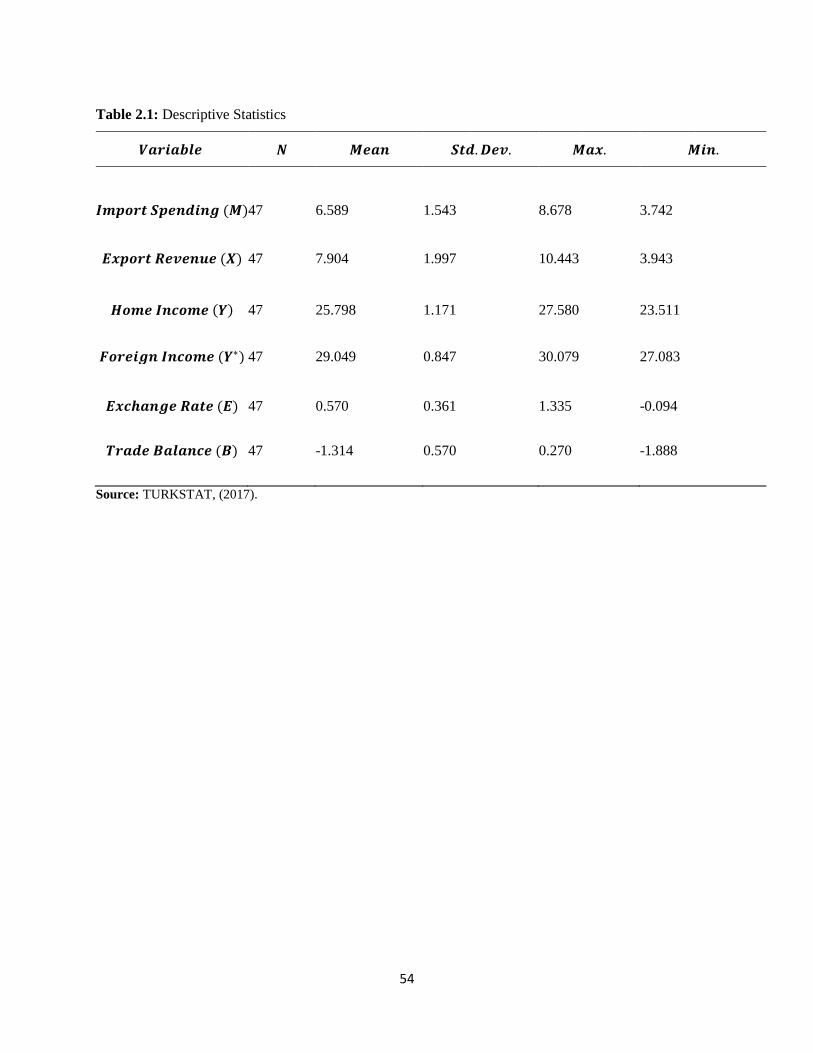
54
Table 2.1: Descriptive Statistics
𝑽𝒂𝒓𝒊𝒂𝒃𝒍𝒆 𝑵 𝑴𝒆𝒂𝒏 𝑺𝒕𝒅. 𝑫𝒆𝒗. 𝑴𝒂𝒙. 𝑴𝒊𝒏.
𝑰𝒎𝒑𝒐𝒓𝒕 𝑺𝒑𝒆𝒏𝒅𝒊𝒏𝒈 (𝑴) 47 6.589 1.543 8.678 3.742
𝑬𝒙𝒑𝒐𝒓𝒕 𝑹𝒆𝒗𝒆𝒏𝒖𝒆 (𝑿) 47 7.904 1.997 10.443 3.943
𝑯𝒐𝒎𝒆 𝑰𝒏𝒄𝒐𝒎𝒆 (𝒀) 47 25.798 1.171 27.580 23.511
𝑭𝒐𝒓𝒆𝒊𝒈𝒏 𝑰𝒏𝒄𝒐𝒎𝒆 (𝒀∗) 47 29.049 0.847 30.079 27.083
𝑬𝒙𝒄𝒉𝒂𝒏𝒈𝒆 𝑹𝒂𝒕𝒆 (𝑬) 47 0.570 0.361 1.335 -0.094
𝑻𝒓𝒂𝒅𝒆 𝑩𝒂𝒍𝒂𝒏𝒄𝒆 (𝑩) 47 -1.314 0.570 0.270 -1.888
Source: TURKSTAT, (2017).
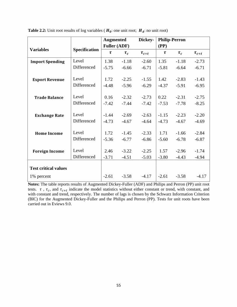
55
Table 2.2: Unit root results of log variables ( 𝑯𝟎: one unit root; 𝑯𝑨: no unit root)
Variables
Specification
Augmented Dickey-
Fuller (ADF)
Philip-Perron
(PP)
𝝉 𝝉𝒄 𝝉𝒄+𝒕 𝝉 𝝉𝒄 𝝉𝒄+𝒕
𝐈𝐦𝐩𝐨𝐫𝐭 𝐒𝐩𝐞𝐧𝐝𝐢𝐧𝐠 Level 1.38 -1.18 -2.60 1.35 -1.18 -2.73
Differenced -5.75 -6.66 -6.71 -5.81 -6.64 -6.71
𝐄𝐱𝐩𝐨𝐫𝐭 𝐑𝐞𝐯𝐞𝐧𝐮𝐞 Level 1.72 -2.25 -1.55 1.42 -2.83 -1.43
Differenced -4.48 -5.96 -6.29 -4.37 -5.91 -6.95
𝐓𝐫𝐚𝐝𝐞 𝐁𝐚𝐥𝐚𝐧𝐜𝐞 Level 0.16 -2.32 -2.73 0.22 -2.31 -2.75
Differenced -7.42 -7.44 -7.42 -7.53 -7.78 -8.25
𝐄𝐱𝐜𝐡𝐚𝐧𝐠𝐞 𝐑𝐚𝐭𝐞 Level -1.44 -2.69 -2.63 -1.15 -2.23 -2.20
Differenced -4.73 -4.67 -4.64 -4.73 -4.67 -4.69
𝐇𝐨𝐦𝐞 𝐈𝐧𝐜𝐨𝐦𝐞 Level 1.72 -1.45 -2.33 1.71 -1.66 -2.84
Differenced -5.36 -6.77 -6.86 -5.60 -6.78 -6.87
𝐅𝐨𝐫𝐞𝐢𝐠𝐧 𝐈𝐧𝐜𝐨𝐦𝐞 Level 2.46 -3.22 -2.25 1.57 -2.96 -1.74
Differenced -3.71 -4.51 -5.03 -3.80 -4.43 -4.94
Test critical values
1% percent -2.61 -3.58 -4.17 -2.61 -3.58 -4.17
Notes: The table reports results of Augmented Dickey-Fuller (ADF) and Philips and Perron (PP) unit root
tests. 𝜏 , 𝜏𝑐, and 𝜏𝑐+𝑡 indicate the model statistics without either constant or trend, with constant, and
with constant and trend, respectively. The number of lags is chosen by the Schwarz Information Criterion
(BIC) for the Augmented Dickey-Fuller and the Philips and Perron (PP). Tests for unit roots have been
carried out in Eviews 9.0.

56
Table 2.3: VAR lag order selection criteria
Lag
Order
Model 1 Model 2 Model 3
AIC SIC HQC AIC SIC HQC AIC SIC HQC
0 3.795 3.918 3.840 4.544 4.667 4.589 3.230 3.394 3.291
1 -3.945* -3.454* -3.764* -2.288 -1.796* -2.106* -5.610* -4.791* -5.530*
2 -3.904 -3.044 -3.587 -2.366* -1.506 -2.049 -5.475 -4.000 -4.931
3 -3.799 -2.571 -3.346 -2.025 -0.796 -1.572 -5.167 -3.037 -4.381
4 -3.891 -2.294 -3.302 -2.080 -0.483 -1.491 -5.210 -2.424 -4.183
Notes: *Indicates the smallest value of the criterion. AIC, Akaike Information Criterion; SIC, Schwarz Information
criterion; HQ, Hannan-Quinn Information Criterion.

57
Table 2.4: Results of Johansen’s maximum likelihood tests for multiple co-integrating relationships
Model 1 Model 2 Model 3
Null
Hypothesis Test-Stat P-value Test-Stat P-value Test-Stat P-value
Trace test
𝑁𝑜𝑛𝑒 (𝑟 = 0) 35.576 0.0696 29.971 0.0877 58.772 0.0634
𝐴𝑡 𝑚𝑜𝑠𝑡 1 (𝑟 ≤ 1) 15.494 0.1133 14.589 0.0681 28.682 0.0668
𝐴𝑡 𝑚𝑜𝑠𝑡 2 (𝑟 ≤ 2) 3.841 0.1009 4.364 0.0767 7.721 0.4957
Maximum
Eigenvalue
Test
𝑁𝑜𝑛𝑒 (𝑟 = 0) 16.406 0.2020 15.381 0.2630 30.089 0.0733
𝐴𝑡 𝑚𝑜𝑠𝑡 1 (𝑟 ≤ 1) 12.690 0.0873 10.224 0.1976 20.961 0.0528
𝐴𝑡 𝑚𝑜𝑠𝑡 2 (𝑟 ≤ 2) 6.480 0.1109 4.364 0.0722 6.949 0.4952
Source: Author’s computation from the data using Eviews 9.

58
Table 2.5: Export variance decomposition analysis
𝒌 𝒔. 𝒆. 𝒙𝒕 𝒓𝒕 𝒚𝒕
1 0.189 100.000 0.0000 0.0000
2 0.253 99.222 0.634 0.143
3 0.294 97.613 1.794 0.591
4 0.323 95.327 3.221 1.450
5 0.343 92.497 4.719 2.783
6 0.359 89.264 6.141 4.593
7 0.372 85.781 7.388 6.829
8 0.383 82.200 8.405 9.394
9 0.394 78.661 9.175 12.163
10 0.403 75.278 9.711 15.010
Note: k denotes the forecast horizon in years. Variance decomposition analysis is carried out from a tri-variate
vector autoregressive model with the export revenue ordered first, whereas the foreign income is placed last.
Standard errors (s.e.) are obtained from 5000 nonparametric bootstrap simulations. All results are obtained using
Eviews 9.0.

59
Table 2.6: Import variance decomposition analysis
𝒌 𝒔. 𝒆. 𝒎𝒕 𝒓𝒕 𝒚𝒕
1 0.252 100.000 0.0000 0.0000
2 0.336 99.554 0.268 0.176
3 0.389 98.591 0.742 0.666
4 0.426 97.192 1.291 1.516
5 0.454 95.461 1.822 2.716
6 0.475 93.514 2.277 4.208
7 0.493 91.466 2.630 5.902
8 0.508 89.418 2.880 7.701
9 0.521 87.447 3.039 9.512
10 0.534 85.609 3.126 11.263
Note: k denotes the forecast horizon in years. Variance decomposition analysis is carried out from a tri-variate
vector autoregressive model with the import spending ordered first, whereas the home income is placed last.
Standard errors (s.e.) are obtained from 5000 nonparametric bootstrap simulations. All results are obtained using
Eviews 9.0.

60
Table 2.7: Trade balance variance decomposition analysis
𝒌 𝒔. 𝒆. 𝒃𝒕 𝒓𝒕 𝒚𝒕 𝒚𝒕∗
1 0.230 100.000 0.0000 0.0000 0.0000
2 0.257 98.184 1.116 0.680 0.018
3 0.267 95.511 2.872 1.583 0.032
4 0.274 92.915 4.681 2.366 0.036
5 0.279 90.710 6.295 2.957 0.035
6 0.283 88.929 7.652 3.383 0.035
7 0.286 87.515 8.759 3.686 0.038
8 0.288 86.402 9.648 3.902 0.046
9 0.290 85.527 10.353 4.060 0.058
10 0.292 84.841 10.905 4.176 0.076
Note: k denotes the forecast horizon in years. Variance decomposition analysis is carried out from a quad -variate
vector autoregressive model with an ordering, the trade balance, the exchange rate, the home and foreign income.
Standard errors (s.e.) are obtained from 5000 nonparametric bootstrap simulations. All results are obtained using
Eviews 9.0.

61
Figure 2.1: Variable series.
3
4
5
6
7
8
9
70 75 80 85 90 95 00 05 10 15
Import Spending
2
4
6
8
10
12
70 75 80 85 90 95 00 05 10 15
Export Revenue
23
24
25
26
27
28
70 75 80 85 90 95 00 05 10 15
Domestic Income
27
28
29
30
31
70 75 80 85 90 95 00 05 10 15
Foreign Income
-2.0
-1.5
-1.0
-0.5
0.0
0.5
70 75 80 85 90 95 00 05 10 15
Trade Balance
-0.4
0.0
0.4
0.8
1.2
1.6
70 75 80 85 90 95 00 05 10 15
Exchange Rate
Source: TURKSTAT, (2017)

62
Figure 2.2: Impulse Response Function Estimates of Export Revenue
(a) (b)
-.2
-.1
.0
.1
.2
.3
1 2 3 4 5 6 7 8 9 10
Percentage responses to a 1% Exchange Rate shock
-.2
-.1
.0
.1
.2
.3
1 2 3 4 5 6 7 8 9 10
Percentage responses to a 1% Foreign Income shock
(c)
-.2
-.1
.0
.1
.2
.3
1 2 3 4 5 6 7 8 9 10
Percentage responses to a 1% Foreign Demand shock
Note: Impulse-response functions are obtained from a tri-variate vector autoregressive model
with the exchange rate ordered first, whereas the foreign demand variable is placed last.

63
Figure 2.3: Impulse Response Function Estimates of Import Spending
(a) (b)
-.2
-.1
.0
.1
.2
.3
.4
1 2 3 4 5 6 7 8 9 10
Percentage responses to a 1% Exchange Rate shock
-.2
-.1
.0
.1
.2
.3
.4
1 2 3 4 5 6 7 8 9 10
Percentage responses to a 1% Home Income shock
(c)
-.2
-.1
.0
.1
.2
.3
.4
1 2 3 4 5 6 7 8 9 10
Percentage responses to a 1% Home Demand shock
Note: Impulse-response functions are obtained from a tri-variate vector autoregressive model with the
exchange rate ordered first, whereas the home demand variable is placed last.

64
Figure 2.4: Impulse Response Function Estimates of Trade Balance
(a) (b)
-.2
-.1
.0
.1
.2
.3
1 2 3 4 5 6 7 8 9 10
Percentage responses to a 1% Exchange Rate shock
-.2
-.1
.0
.1
.2
.3
1 2 3 4 5 6 7 8 9 10
Percentage responses to a 1% Foreign Income shock
(c) (d)
-.2
-.1
.0
.1
.2
.3
1 2 3 4 5 6 7 8 9 10
Percentage responses to a 1% Home Income shock
-.2
-.1
.0
.1
.2
.3
1 2 3 4 5 6 7 8 9 10
Percentage responses to a 1% Trade Balance shock
Note: Impulse-response functions are obtained from a quad-variate vector autoregressive model with
ordering of the exchange rate, the home income, the foreign income, and the trade balance.

65
Essay 3: The Causal Effect of Education on Poverty: Evidence from Turkey
Introduction
Since poverty is a multifaceted concept involving economic, social, and political elements, there
is no unique definition of poverty. The concept of poverty differs from country to country in
terms of level of development and how it is viewed by people. The United Nations (1998)
identifies it as “… the inability of getting choices and opportunities, a violation of human
dignity” (UN Statement, June 1998, signed by the heads of all UN agencies) whereas the World
Bank (2000) defines poverty as “poverty is pronounced deprivation in wellbeing and comprises
many dimensions” (World Bank, 2000, p.15). In the existing literature, poverty is measured by
various methods such as the absolute poverty approach, relative poverty approach, and subjective
poverty approach.
Poverty posits challenges to education since lower levels of educational attainment are
typical of students raised in poverty. Lower academic achievement among high concentrations of
poor students is supported by insufficient funding, weakened parental support, and higher teacher
turnover caused by inadequate school resources and lower opportunities for teachers’
professional development (Blazer and Romanik, 2009). Therefore, poverty deprives children of
the choice of educational opportunities and reduces educational outcomes (Coley and Baker,
2013). Even before going to school impoverished children may not acquire the social skills
necessary for studying due to situations in the family, for example, parental inconsistency and

66
a lack of support for children (Ferguson et al., 2007). The deficiencies continue through
postgraduate training so poverty has a negative effect on academic achievement.
There has been ongoing debate about the links between poverty and the level of
education. Poverty and educational attainment are closely intertwined. Investment in education
reduces the risk of poverty through enhancing the wages or income as well as people’s
productivity. In addition, education allows people to obtain some necessary skills which promote
their capacity to produce more effectively. On the other hand, poverty limits the quality of
education and equal access to education by affecting the resources to students. (Chaudhry and
Rehman, 2009). As a result, poverty and education are inversely related to each other.
The rest of the paper is structured as follows. The next section presents the previous
literature about the relationship between education and poverty. Section 3 discusses potential
endogeneity problem. Section 4 describes data, provides definitions of the main constructed
variables and presents results of descriptive statistics. Section 5 discusses the estimation
methodologies used in this study. Main findings are presented in Section 6. Section 7
summarizes the main conclusions.
Literature Review
Education plays an important role in combating poverty as it prepares poor people for the
competitive labor market (Blustein et al., 2014). Graduates are able to lead productive lives since
education aims to equalize economic opportunity in the country by offering a route out of
poverty for the disadvantaged (Coley and Baker, 2013; Raffo, et al., 2007). Educational
initiatives which mean to close the poverty achievement gap by providing student assessments
face obstacles linked to accountability for student achievement without controlling all the factors
67
so educational institutions are incapable of eliminating inequalities completely (Blazer and
Romanik, 2009; Lacour and Tissington, 2011).
Despite poverty being a major obstacle to lack of knowledge, education remains the key
to success. Education and poverty are closely linked. Over the past decades, students without full
education backgrounds have had lifelong struggles. Biddle (2014) defines poverty as the lack of
food, shelter, education, information.
Numerous studies have been performed on the direct impact of poverty on education.
These studies often lack economic theory, and instead take an ad hoc approach. Black et al.
(2013) argue outcomes for children age 4 to 15 are directly proportional to parents’ income and
also that cognition is negatively affected by lower income. For example, parents from poor
backgrounds are likely to give birth to premature children and the premature children are at
higher risks of failure in school as compared to those born in middle or higher income families.
Educating a girl child is said by some to be the first step to eliminating poverty in a
nation. Lampert and Burnett (2015) argue that educating girls on their rights concerning
marriages and responsive health care empowers them, improving their decision making towards
early pregnancies that can terminate their education process. The problem is poverty makes it
hard for these girls to get that knowledge, leading to most of them dropping out of school.
Similarly, Mihai et al. (2015) found that when girls stay longer in school, it lowers the
chances of early marriages. Staying longer in an educational environment improves their success
rates of being rewarded with good jobs after school. They also added that for developing nations
with high levels of poverty, these girls may leave school and fail to get jobs since the
government is not in a position of employing all the graduates.

68
In addition, Schwill et al. (2014) note that children learn hygiene in primary school since it is
there where they are taught causes, symptoms, and the dangers of illnesses including HIV.
Without this knowledge, students including those who had a chance to finish school and educate
the community may perish from preventable diseases.
A study by Rolleston (2011) investigated the linkage between school attendance, welfare
and poverty in Ghana over the period 1991-2006 using the Ghana Living Standards Surveys.
This case study found that increased educational access plays an important role in determining
household welfare. Lastly, Cannon (2015) and Burn and Childs (2016) reported that poverty is
associated with the learning environment. Students from well-developed urban areas will be in a
better position to access good quality education and an organized infrastructure as compared to
those from less developed areas. In a well-structured environment, studies show that other than
academics, activities such as soccer and swimming games improve students’ concentration and
reading during class time. However typically only institutions in areas where most of the
population is above the poverty line will afford this service.
The literature on the association between poverty and education in Turkey is limited and
these studies do not take the endogeneity problem into account. For example, Kizilgol and
Ucdogruk (2011) investigate the link between poverty and household living standards using the
Household Budget Surveys over the period from 2002-2006 by applying the Heckman selection
model. In this study, they find that the probability of falling into poverty decreases with the
household head's education. In other words, the higher the education access of the head, the
higher household welfare.
The Household Budget Survey data of 2008 is used by Caglayan and Dayioglu (2011) to
explore the factors that could influence poverty status and living standards of a household in

69
Turkey by employing parametric and semi-parametric logit models. According to the
econometric results, the occupation of the household head, income and working status are the
most important determinants of poverty. Lastly, using a similar dataset, Bilenkisi et. al (2015)
apply logistic regression models to analyze the effect of the household head’s educational
attainment on poverty risk. Their empirical findings highlight that there is a negative relationship
between the head of household’s education level and the risk of poverty. Household poverty is
higher among female-headed households compared to male-headed households because of low
education.
Potential Endogeneity Problem
There are numerous explanations for why education may be endogenous to poverty, among them
the idea that a proper investment in educational attainment in early life may have a consequence
on both poverty in later life and further education in the future. Additionally, other variables such
as social activities away from school, the child’s ability, the background of a person’s family as
well as time preferences may concurrently influence poverty and education (Engle and Black,
2008). At the same time, just as there may be reverse causality resulting from education to
poverty, there may equally be a causality from poverty to education. For example, investment in
education reduces poverty through enhancing the wages or income as well as people’s
productivity. In addition, education allows people to obtain some necessary skills which promote
their capacity to produce more effectively. On the other hand, poverty limits the quality of
education and equal access to education by affecting the resources to students (Chaudhry and
Rehman, 2009). As a result, poverty and education are inversely related to each other. Therefore,
we estimate IV models where education is instrumented by several instrumental variables.

70
First instrument is the Turkish educational reform, which made in 1960s. This instrument is
similar to the one used by Tansel and Karaoglan (2016) for their analysis of health and education
in Turkey. In the early 1960s, the Turkish government made numerous changes in the
educational sector. For instance, in January, 1961, there was a law passed that increased the
mandatory schooling program from three to five years in the villages (Erdogan, 2003; Sen,
2013). Additionally, in 1960, a law allowed the graduates from middle schools to teach in the
primary schools, while the higher graduates would teach in the middle schools after successfully
completing teaching training courses. Consequently, these new laws increased the number of
teachers and schools in the country (Akyuz, 2007). Following Tansel and Karaoglan (2016), we
calculate the average years of schooling based on the Ministry of Education statistics1. If a
household head completed primary school in 1952 or later, the years of schooling is equal to 5.
Thus, the instrumental variable, 𝑅𝑒𝑓𝑜𝑟𝑚1961, takes the value of one if the household head was
born in 1952 or later, and it is zero if the household head was born before 1952.
The second instrument is constructed based on the 1997 Compulsory Schooling reform.
The Turkish parliament passed a law in 1997 to increase the mandatory years of schooling from
5 to 8 years. Exposure to this reform is used as an instrument for completed schooling to analyze
the effect of education on various poverty outcomes. The instrumental variable, 𝑅𝑒𝑓𝑜𝑟𝑚1997,
takes the value of one if the household head was born after 1986, and it is zero if the household
head was born before 1986. However, it uncertain whether those who were born in 1986 were
exposed by the reform because of education system in Turkey (Cesur et al., 2014).
1 The average years of schooling for primary school graduates prior to 1952 is calculated as a weighted average of
three and five years of schooling where the weights are the number of rural and urban primary school graduates
respectively. (Tansel and Karaoglan (2016)).

71
Data and Definitions of Variables
Data
To analyze the impact of education attainment on poverty, this study uses cross-sectional data
obtained from the Turkish Statistical Institute’s (TURKSTAT) Income and Living Conditions
Survey (hereafter, ILCS) which took place in 2013. The ILCS is a nationally representative
survey repeated each year. The purpose of the survey is to monitor the indicators on income
distribution, poverty, social exclusion, labor status, demographical characteristics, educational
and health status of household members. The 2013 ILCS was performed with face-to-face
interviews between April 2013 and July 2013, applying a two-stage stratified random sampling
approach (with household as the cluster unit, and all members of the household over 15 years of
age interviewed). The first-stage sampling unit considers the household whose members continue
to live at the same address as in the previous application and also new households. The second-
sampling unit includes sample persons who have moved to another dwelling and households that
have moved to another address. The original sample consists of 19,899 households, 6,671 of
which were from rural areas and 13,228 of which were from urban areas. The survey covers the
entire country and the target population comprises all persons residing within the borders of the
republic of Turkey. The survey excludes the institutionalized population in the dormitories,
guesthouses, childcare centers, orphanages, nursing homes, private hospitals, prisons, and
military barracks.
Dependent Variable
Our objective is to identify the linkages between household characteristics and poverty. The key
outcome variable, poverty, is constructed based on the “relative poverty approach” which is
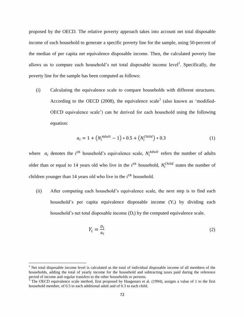
72
proposed by the OECD. The relative poverty approach takes into account net total disposable
income of each household to generate a specific poverty line for the sample, using 50-percent of
the median of per capita net equivalence disposable income. Then, the calculated poverty line
allows us to compare each household’s net total disposable income level2. Specifically, the
poverty line for the sample has been computed as follows:
(i) Calculating the equivalence scale to compare households with different structures.
According to the OECD (2008), the equivalence scale3 (also known as ‘modified-
OECD equivalence scale’) can be derived for each household using the following
equation:
𝑎𝑖 = 1 + (𝑁𝑖𝐴𝑑𝑢𝑙𝑡 − 1) ∗ 0.5 + (𝑁𝑖
𝐶ℎ𝑖𝑙𝑑) ∗ 0.3 (1)
where 𝑎𝑖 denotes the 𝑖𝑡ℎ household’s equivalence scale, 𝑁𝑖𝐴𝑑𝑢𝑙𝑡 refers the number of adults
older than or equal to 14 years old who live in the 𝑖𝑡ℎ household, 𝑁𝑖𝐶ℎ𝑖𝑙𝑑 states the number of
children younger than 14 years old who live in the 𝑖𝑡ℎ household.
(ii) After computing each household’s equivalence scale, the next step is to find each
household’s per capita equivalence disposable income (Yi) by dividing each
household’s net total disposable income (Di) by the computed equivalence scale.
𝑌𝑖 =𝐷𝑖
𝑎𝑖 (2)
2 Net total disposable income level is calculated as the total of individual disposable income of all members of the
households, adding the total of yearly income for the household and subtracting taxes paid during the reference
period of income and regular transfers to the other households or persons. 3 The OECD equivalence scale method, first proposed by Haagenars et al. (1994), assigns a value of 1 to the first
household member, of 0.5 to each additional adult and of 0.3 to each child.

73
(iii) The last step is to find the poverty line by taking fifty-percent of the median
household per equivalence disposable income set. The poverty line is written as:
𝑃𝑜𝑣𝑒𝑟𝑡𝑦 𝑙𝑖𝑛𝑒 = 𝑚𝑒𝑑𝑖𝑎𝑛 𝑜𝑓 (𝑌1,𝑌2, … , 𝑌𝑖 ∗ 0.50 (3)
Following these calculations, the dependent variable in logistic regression analysis is determined
as follow: If a head of household per equivalence disposable income is less than the calculated
relative poverty line, the variable is coded 1 which indicates poor households, otherwise non-
poor. The value of the computed poverty line for Turkey is 5276.86 Turkish Liras based on
equation (3).
A person’s prosperity is defined not only by the goods that she can afford, but also by
the comparison to what other members of society can afford. The comparison of what people
can afford with regards to what other people can be expected to afford is made through the
relative poverty analysis (Iceland, 2005). To find whether a person is relatively poor, her well-
being is compared to the objective measure determined by the researcher – the average standard
of living. According to Alcock (1998), relative poverty requires value judgment to determine
whether one is poor compared to others and, thus, is subjective.
Relative poverty concerns the economic status of a person compared to other society
members. It shows whether a person lacks consumption, income, housing of appropriate quality,
clothing, and other material possessions compared to others (Iceland, 2005). The relative
poverty line is determined in each region considering the distribution of consumption, income,
housing, or material possessions in this region. According to Woolard and Leibbrandt (1999) for
developed countries, the relative poverty line should be established at half of the country’s
average consumption, income, or other characteristics mentioned above. Accordingly, those
74
who fall below this line are classified as relatively poor and those who fall above this line are
classified into “not poor” category.
Relative poverty is often criticized for its consideration only of the objectively set
consumption and income levels. However, those who fall into the category “poor” may actually
not feel themselves poor, while those falling into the “not poor” category may, in fact, feel poor.
The Methodologies and Models
This study aims to analyze the relationship between education and poverty using various
econometric techniques including Ordinary Least Squares (OLS), Linear Probability Model
(LPM), Logit and Probit Models, and Instrumental Variable (IV) Probit Model. Each method
depends on a different set of assumptions and highlights various aspects of the underlying
processes of determining the impact of education on poverty.
In the application of the OLS model, we use a continuous dependent variable. Following
Mincer (1994) a standard model is based on the human capital earnings function can be written
as follows:
𝐼𝑛𝑌𝑖 = 𝑋𝑖𝛽 + 휀𝑖 (4)
where 𝐼𝑛𝑌𝑖 is the natural logarithm of per relative income for observation i, and 𝑋𝑖 is a vector of
individual characteristics including age, age squared, gender, marital status, education level, and
working status. 𝛽 is the vector of unknown parameters to be estimated, and 휀𝑖 is a random
disturbance term, which is assumed to satisfy the usual properties of mean zero and constant
variance.
In the case of the variable explained in the model is binary, we use the liner probability
model, logit model and probit model to analyze the relationship between the level of educational

75
attainment and poverty. In such cases, the outcome variable takes a value of one when the head
of household is poor and the value of zero otherwise. The LPM is simple to estimate and use
OLS for a regression., where the dependent variable is a binary variable instead of continuous.
The structural model is
𝑦𝑖 = 𝑥𝑖𝛽 + 휀𝑖 (5)
where 𝑥𝑖 is a vector of values for the i-th observation, 𝛽 is a vector of parameters, and the 휀 is
the error term. The LPM predicts the probability of an event occurring, for example, y=1 if a
household head is poor, and y=0 otherwise. Although the LPM is easy to estimate and interpret,
it has some shortcomings. First, it violates the OLS assumptions such as heteroscedasticity and
normality. Second, the linear probability model can produce out of range predictions.
We also used binomial logit and probit models to analyze the impacts of educational level
on the poverty risk. As with LPM, these models also use a binary dependent variable. The
difference between the LPM and probit and logit model are: (i) predicted probabilities in both
probit an d logit models are limited between 0 and 1, (ii) probit model assumes 휀𝑖 is normal, (iii)
these models cannot be estimated by OLS.
In the logit and probit regressions, we focus on the marginal effects rather than on the
coefficients. Sekyere and Chiaraah (2014, pp. 32) states that “the marginal effect which is
analogous to the elasticity gives the percentage change in the probability of a success in response
to a percent change in the explanatory variable”. From our results, the coefficient signs for
variables and marginal effects are consistent with the probit and logit models that imply we have
an economic meaning. Moreover, the probit and logit models produce almost identical marginal

76
effects (Katchova, 2013). Probit and logit models are estimated using the Maximum Likelihood
Method (MLE). The logit and probit models can be expressed as follows:
For the logit model,
𝐹(𝑥′𝛽) = Ω(𝑥′𝛽) =𝑒𝑥′𝛽
1+𝑒𝑥′𝛽=
exp(𝑒𝑥′𝛽)
1+𝑒𝑥′𝛽) (6)
where 𝐹(𝑥′𝛽) is the cdf of the logistic distribution.
For the logit model,
𝐹(𝑥′𝛽) = ∅(𝑥′𝛽) = ∫ ∅(𝑧)𝑑𝑧𝑥′𝛽
−∞ (7)
where 𝐹(𝑥′𝛽) is the cdf of the standard normal distribution.
However, the association between the probability of outcome variable and a specific variable is
interpreted by means of the marginal effect, which is computed as follow:
ф[𝑠(𝑋)]
𝑋𝑚= ∅(𝑠).
𝜕𝑠
𝜕𝑋𝑚= ∅(𝑠)(𝑎𝑚 + ∑ 𝑏𝑚𝑖𝑋𝑖
𝑘𝑖=1 ) (8)
The marginal effects provide insights into how the explanatory variables shift the probability of
frequency of falling into poverty.
Lastly, we used IV-probit model to deal with endogeneity problem between education
and poverty. As discussed above, poverty and education are inversely related to each other.
Therefore, we estimate IV models where education is instrumented by several instrumental
variables. IV regression is a powerful tool to analyze causal effects. In practice, finding good
instrument is the most difficult aspect IV estimation. Using invalid instruments produce
meaningless results. It therefore is important to assess whether a given set of instruments is valid

77
in an econometric model. If the instruments are weak, then the normal distribution provides a
poor approximation to the sampling distribution of the Two Stage Least Squares (TSLS)
estimator, even if the sample size is large. In fact, if instruments are weak, then the TSLS
estimator can be badly biased in the direction of the OLS estimator. That is, TSLS is no longer
reliable in the case of weak instrument. To test an instrument is ‘reliable’, we use the first-stage
F-statistic, which is testing the hypothesis that the coefficients on the instruments equal zero in
the first stage of TSLS. In the case of one instrument and one endogenous regressor, if the F-
statistics from the first-stage regression exceeds 10, we have sufficiently strong instrument for
the case of exactly-identified case (Stock and Watson, 2011).
In this study, we use two different instruments such as the Turkish educational reform in
1960s and the 1997 Compulsory Schooling Reform. To address endogeneity of educational
attainment, we estimate an IV-probit model depicted by Equation (9) below,
𝑃𝑜𝑣𝑖 = 𝛽0 + 𝛽1𝐸𝑑𝑢𝑐𝑖 + 𝑋𝑖𝛿 + 휀𝑖 (9)
where the variable 𝑃𝑜𝑣𝑖 has two different outcomes. First, it is a continuous variable and defined
as the natural logarithm of per capita relative income. Second, it is a binary variable and denotes
whether the household’s per equivalence disposable income is below the calculated poverty line
or not. Therefore, in this case, 1 indicates the head of household is poor and 0 indicates
otherwise. 𝐸𝑑𝑢𝑐𝑖 is an indicator to state the years of schooling of the household’s head. The
vector, X, stands for personal characteristics of the household head, including age, gender,
marital status, and employment status. Equation (9) is the expression of the second-stage
regression in IV-probit model.

78
Since poverty and educational attainment are closely intertwined, estimating equation (9) by
Ordinary Least Square (OLS) could lead to biased results because of unobserved determinants
that may affect the risk of poverty. Alternatively, reverse causality may exist and poverty may
influence the level of education attainment. To solve the endogeneity of educational attainment,
we use different Education Reforms implemented in Turkey as an instrument. The first-stage of
IV-probit model can be expressed as follow:
𝐸𝑑𝑢𝑐𝑖 = 𝛼0 + 𝛼1𝐸𝑑𝑢𝑐𝑎𝑡𝑖𝑜𝑛𝑎𝑙𝑅𝑒𝑓𝑜𝑟𝑚𝑖 + 𝑋𝑖𝜗 + 𝜇𝑖 (10)
where 𝐸𝑑𝑢𝑐𝑎𝑡𝑖𝑜𝑛𝑎𝑙𝑅𝑒𝑓𝑜𝑟𝑚 is a dummy variable that indicates whether the household head was
affected by the reform or not.
Estimation Results
Summary Statistics
To avoid the problem of perfect multicollinearity, one classification is dropped from each group
of variables for estimation purposes. Table 3.1 and Table 3.2 provide the choice of explanatory
variables and their summary statistics, respectively. From Table 3.2, the set of socio-economic
and demographic characteristics contains the following variables: Female, which is coded 1 if
the individual is female and 0 otherwise. On average, 15% of the individuals in the rural area are
female whereas it is 16% in the urban area.
Age measures the age of the individuals of the sample. To test nonlinearity between
income and age, we also introduce the variable age squared (𝐴𝑔𝑒2 ). The average age in the
rural area 53 years, while it is 47 years in the urban area.

79
Marital status is measured by three dummies indicating whether the individual has married
(Married), has never married (Single), has divorced or separated or widowed (Divorced--
Widowed - Separated). The reference variable is whether the individual is single. In the sample
of urban area, 81% of the individuals are married, 4% of the individuals are single (never
married), and 15% of the individuals are divorced or widowed or separated. This corresponding
numbers for urban area are 81%, 3%, and 16%.
We define four dummies to control for individuals’ labor market status. The variable
Working takes the value 1 if the individual is working. The dummy Retired is coded 1 if the
individual is retired. The Inactive dummy takes the value 1 when the individual reports being a
seasonal worker, busy with household chores and student. The reference variable is whether the
individual is not working in a paid job (Unemployed). In the urban sample, 63% the individuals
are working, 4% are unemployed, 13% are retired, 20% are inactive in the labor force. The labor
market structure in the urban area tends to be quite similar to the rural area.
We define the Educational level as a qualitative variable with five categories: ‘Illiterate,’
‘Primary School degree,’ ‘Secondary School degree,’ ‘High School degree’ and ‘University
degree or above’. In the sample of rural area, 28% of the individuals are illiterate, 52% have
completed primary school, 8% have completed secondary school, 7% have completed high
school and 5% have university studies.
OLS Estimation Results
Table 3.3 presents the robust OLS estimation results of the logarithmic relative income equation
(4) ignoring the endogeneity of education. Most of the findings are consistent with expectations
and previous studies. The adjusted-R square for rural and urban areas stand at 0.25 and 0.35,

80
respectively. According to Su and Heshmati (2013), the R-squared value tends to be small in
Mincerian model because of (i) the individual incomes have a large dispersion so that makes
regressions difficult to capture the marginal effects of each variable; (ii) there might be some
unobserved effects that we fail to capture using the selected variables such as ability.
The age variable has a positive impact on the household head’s earnings, with a one-year
increase in age increasing household head’s income 0.02 in both areas, holding other variables
constant. However, age squared is included in the regression to explain the non-linearity of the
variable.
With respect to the gender of the household head, in both areas, the variable’s coefficient
is negative and statistically significant at 1 percent. This implies that per capita household
relative income with a male household is higher than female-headed ones. Statistically, a female-
headed household who lives in rural area is estimated to earn about 22.9% less than male
counterparts.
As presented in Table 3.3, education, as expected, is an important factor in determining
the household head’s relative income. According to the results, all the levels of education are
statistically significant at the 1 percent in both rural and urban areas and it is a crucial part in
increasing household head welfare. This indicates that the higher level of education the
household head, the higher the household per capita relative income. Especially, on average, the
income of the household head with primary education is 41.3% and 42.4% higher compare to
people with no education in rural area and urban area, respectively. Similarly, university diploma
has the greatest impact on income in both area. Having a university diploma, on average,
increases the household head’s income 2.56 percent point in rural area and 2.63 percent point in
urban area.

81
The next variable, marital status of the household head had a negative sign and is significant at
the 1 percent in both areas except the widowed/divorced/separated in urban areas, which is not
statistically significant at any significance level. Statistically, married household head’s income
in rural and urban areas is 24.6% and 14.4% less than those who are single, keeping all other
things the same.
Lastly, we analyzed the relation between employment status of household head and per
capita income. According to the results, being both employed and retired has a positive sign and
are statistically significant at the 1 percent level for both areas, which indicates that per capita
household’s relative income is higher for working and retired household head. Statistically, on
average, being employed and retired is 61.4% and 62% and 63.3% and 53.4% higher compare to
people with unemployed in rural area and urban area, respectively. However, the coefficient of
being inactive (such as, housewife, student) is only statistically significant at the 1 percent in
urban areas.
The Results of LPM, Logit and Probit Models
Table 3.4 presents the regression results based on three different econometric specification. As
discussed above, the linear probability model is simply running OLS for a regression, where the
dependent variable is a binary variable. The interpretation of the coefficients in the LPM is very
straightforward. Because the regression in column (1) and column (4) are a linear probability
model, respectively, for rural and urban sample groups, its coefficients are estimated changes in
predicted probabilities resulting from a unit change in the independent variable. Accordingly,
keeping all other things the same, an increased level of education will reduce the head of
household probability of being poor. More specifically, holding the other variables in column (1)
and column (4) are constant, the probability of falling into poverty for college graduate is 0.303

82
(30.3%) and 0.366 (36.6%) less than for someone with a no educational attainment for the rural
area and urban area, respectively. In short, because the coefficients are all negative and get
bigger as educational attainment increases, the probability of being poor reduces as educational
attainment increases.
The coefficient for being female in regression (1) and (4) is -0.106 and -0.089, indicating
that the difference between poor and non-poor household heads is 10.6 percentage points for the
rural residents and 8.9 percentage points for the urban residents, holding constant the other
variables in the regression, respectively. This is statistically significant at the 1% significance
level.
We do find, however, the condition of the labor force is an important factor for both area
and all types of labor force have statistically significant at the 1% level and negative effect on the
risk of poverty. For example, a retired household head who lives in rural and urban area is
estimated to decrease the probability of being poor by 34.1 and 33.3 percentage points,
respectively.
With respect to the additional regressors, the findings indicate that only being married
have statistically significant negative impacts on the probability of being poor for both rural and
urban group. In addition, the linear probability model shows only urban residents’ poverty risk is
significantly affected by age.
On the other hand, the logit and probit regressions are run to investigate the effect of the
explanatory variables on the likelihood of the household head being poor. We report marginal
effects to assess the magnitude of the factor effect on the likelihood of poverty risk. The estimates
reported in columns (2), column (3), column (5) and column (6) yields similar findings. As can

83
be seen from both specifications, most of the independent variables are statistically significant at
the 1 percent level. More specifically, with respect to the impact of marital status, married head
of households were significantly more likely to poor than single head of households. Also, living
divorced or widowed or separated dummy variable is not statistically significant for both models.
Likewise, the probability of falling to poverty decreases with head of household age.
For both rural and urban group, the results show that educational levels (primary, middle,
high, and college) of the household head significantly fall the probability of being poor for both
rural and urban residents. This is in line with what was expected. More specifically, compared to
the benchmark group (no education) those who have acquired some level of education are less
likely to be poor. People with higher level of educational attainment will have more
opportunities for a better job and subsequently, higher earnings.
Considering the impact of the employment status dummy variables are statistically
significant in both models and areas, with the exception of the inactive dummy. For logit models,
employed household heads 12.7% in rural area and 15.2% in urban area are less likely to be
poor. Similarly, the results of probit models indicate that retired household head who lives in
rural area less likely to be poor, while those who live in urban area more likely to be poor.
Looking at gender, as expected, female-headed households are more likely to be poor
than male-headed households. According to the results, the marginal effects for age-squared,
being divorced, widowed or separated, and inactive working status seem unlikely to impact both
urban and rural residents’ poverty level as the coefficients are statistically insignificant.
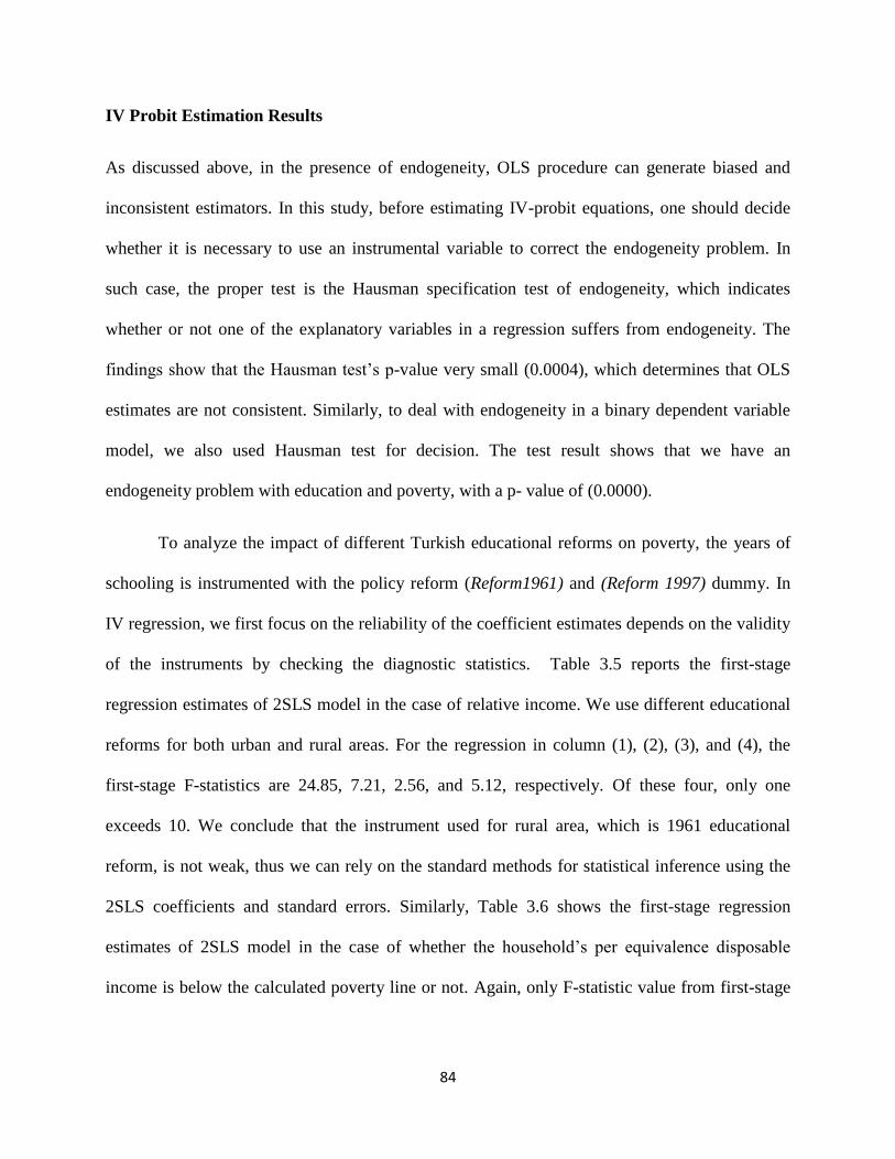
84
IV Probit Estimation Results
As discussed above, in the presence of endogeneity, OLS procedure can generate biased and
inconsistent estimators. In this study, before estimating IV-probit equations, one should decide
whether it is necessary to use an instrumental variable to correct the endogeneity problem. In
such case, the proper test is the Hausman specification test of endogeneity, which indicates
whether or not one of the explanatory variables in a regression suffers from endogeneity. The
findings show that the Hausman test’s p-value very small (0.0004), which determines that OLS
estimates are not consistent. Similarly, to deal with endogeneity in a binary dependent variable
model, we also used Hausman test for decision. The test result shows that we have an
endogeneity problem with education and poverty, with a p- value of (0.0000).
To analyze the impact of different Turkish educational reforms on poverty, the years of
schooling is instrumented with the policy reform (Reform1961) and (Reform 1997) dummy. In
IV regression, we first focus on the reliability of the coefficient estimates depends on the validity
of the instruments by checking the diagnostic statistics. Table 3.5 reports the first-stage
regression estimates of 2SLS model in the case of relative income. We use different educational
reforms for both urban and rural areas. For the regression in column (1), (2), (3), and (4), the
first-stage F-statistics are 24.85, 7.21, 2.56, and 5.12, respectively. Of these four, only one
exceeds 10. We conclude that the instrument used for rural area, which is 1961 educational
reform, is not weak, thus we can rely on the standard methods for statistical inference using the
2SLS coefficients and standard errors. Similarly, Table 3.6 shows the first-stage regression
estimates of 2SLS model in the case of whether the household’s per equivalence disposable
income is below the calculated poverty line or not. Again, only F-statistic value from first-stage

85
regression for rural residents is higher than 10, indicating 1961 educational reform is a
sufficiently strong instrument.
However, column (1) of Table 3.5 and Table 3.6 demonstrate that the educational
expansion increases years of schooling by about 20 and 9 percent for rural residents. In other
words, a household head who were born in or after 1952, the impact of educational expansion on
the years of schooling is positive and the coefficient significant at the one-percent level.
Table 3.7 and Table 3.8 display the second stage results from IV-probit estimation. From
column (1) of Table 3.7, the results suggest that additional years of schooling has a significant
positive impact on a household head’s relative income, which means that an additional years of
schooling increases the head of household who reside in rural area relative income by 7.3
percent. This is the line with what as expected.
Table 3.7 also reports the impact of control variables on the relative income. The married
or divorced dummy variable is statistically significant at the 1%, indicating being married and
divorced decrease a household head’s relative income by 33% and 25%, respectively. With
respect to employment status, being employed or retired has a significant positive affect on
relative income, whereas being inactive is not statistically different from zero. In addition, age
and age-squared variables are statistically significant at the 5%, and relative income increases at
older ages.
On the other hand, column (1) of Table 3.8 presents that an additional years of schooling
has a significant negative impact on the probability of being poor, but this impact is not
statistically significant at any significance level. The coefficient on female is 0.05, indicating that
female-headed households is more likely to be poor. Further, all employment status are

86
statistically significant, which imply that having a job or being retired or inactive reduces the
likelihood of being poor by 3.1%, 3.9% and 0.7%, respectively. In addition, being divorced
significantly falls the probability of being poor for rural residents.
Summary and Conclusion
This paper is the first of its’ kind to use different econometric techniques to analyze the impact
of educational attainment on poverty. We measured poverty level by using relative poverty
approach. In relative poverty approach, we compute the relative poverty line to compare each
household’s net total disposable income. If a household head’s per disposable income falls below the
computed relative poverty line is classified as a poor household head, otherwise not. Yet, relative poverty
approach has some shortcomings. First and foremost, because the poverty line objectively determined by
a researcher, some household heads who fall into the category “poor” may actually not feel themselves
poor, whereas those that are classified as “not poor” may actually feel poor. Therefore, we also use the
relative income, which is the ratio each household’s net total disposable income to the computed
equivalence scale. In such case, we have a continuous outcome for poverty.
In this study, we identified various factors such as levels of education of the household
head, gender of the household head, age of the household head, employment status of the
household head, marital status of the household head as statistically significant determinants of
relative income and the probability of being poor.
To address the endogeneity problem, we instrument the educational level using the
Turkish educational reform, which were implemented in 1961. The findings reveal that the
educational expansion increases years of schooling by about 20 and 9 percent for rural residents.
Moreover, the results also suggest that additional years of schooling has a significant positive

87
impact on a household head’s relative income, which means that an additional years of schooling
increases the head of household who reside in rural area relative income by 7.3 percent

88
References
Aaberge, R., and Brandolini, A. (2014). “Multidimensional poverty and inequality” (Working
paper 976). Printing & Publishing Division of the Banca d’Italia.
Akyüz,Y. (1999). “Türk Eğitim Tarihi (Başlangıçtan 1999’a).” (The History of Turkish
Education from the Beginning until 1999). Alfa Yayınevi. İstanbul.
Alcock, P. (1997). Understanding Poverty. 2nd Edition. Basingstoke: McMillan.
Black, R. E., Victora, C. G., Walker, S. P., Bhutta, Z. A., Christian, P., De Onis, M., ... & Uauy,
R. (2013). “Maternal and child undernutrition and overweight in low-income and middle-
income countries.” The lancet, 382(9890), 427-451.
Blazer, C., and Romanik, D. (2009). “The effect of poverty on student achievement.”
Information Capsule: Research Services, 0901, 1-23.
Biddle, -B. (2014). “Social class, poverty and education.” Routledge.
Blustein, D. L., Kenny, M. E., & Kozan, S. (2014). “Education and work as human birthrights:
Eradicating poverty through knowledge, innovation, and collaboration.” In United
Nations Development Program (Ed.), Barriers to and opportunities for poverty reduction:
Prospects for private sector led interventions (pp. 38-62). Istanbul: UNDP Istanbul Center
for Private Sector in Development.
Burn, K., and Childs, A. (2016). “Responding to poverty through education and teacher
education initiatives: a critical evaluation of key trends in government policy in England
1997-2015.” Journal of Education for Teaching, 42(4), 387-403.
Çağlayan, E., and Dayıoğlu, T. (2011). “Comparing the parametric and semiparametric logit
models: Household poverty in Turkey.” International Journal of Economics and
Finance, 3(5), 197-207.
Cannon, W. B. (2015). “Enlightened Localism: A Narrative Account of Poverty and Education
in the Great Society.” Yale Law & Policy Review, 4(1), 3.
Cesur, R., B. Dursun, and N. Mocan. (2014). “The Impact of Education on Health and Health
Behavior in a Middle-Income, Low-Education Country.” NBER Working Papers 20764.

89
Chaudhry I. S. and Rahman S. (2009). “The impact of gender inequality in education on rural
poverty in Pakistan: An empirical analysis.” European J. Econ. Fin. Admin. Sci. 15:174-
188.
Coley, R. J., and Baker, B. (2013). “Poverty and education: Finding the way forward.” Princeton:
ETS Center for Research on Human Capital and Education.
Engle, P.L. and Black, M.M. (2008). “The effect of Poverty on Child Development and
Educational Outcomes.” Annals of the New York Academy of Sciences, 1136, 243–256.
Erdoğan, İ. (2003). “Yeni bir Binyıla Doğru Türk Eğitim Sistemi Sorunlar ve Çözümler”
(Towards the New Millennium the Turkish Educational System: Problems and
Solutions). Sistem Yayıncılık. İstanbul.
Gadotti, M. (2008). “Education for sustainability: A critical contribution to the Decade of
Education for Sustainable Development.” Green Theory & Practice: The Journal of
Ecopedagogy, 4(1), 1-12.
Hussain, M. D., Bhuiyan, A. B., Said, J., & Halim, M. S. B. A. (2017). “Entrepreneurship
education is the key contrivance of poverty alleviation: An empirical review.” MAYFEB
Journal of Business and Management,1, 32-41.
Iceland, J. (2005). Measuring Poverty: Theoretical and Empirical Considerations.
Measurement. 3(4): 207-243.
Katchova, A. (2013). Probit and Logit Models.’ Econometrics Academy.
Kızılgöl, Ö. A., and Demir, Ç. (2010). “Türkiye’de yoksulluğun boyutuna ilişkin ekonometrik
Analizler (Econometric analyses of poverty dimension in Turkey).” Business and
Economics Research Journal, 1(1), 21-3.
Lampert, J., & Burnett, B. (Eds.) (2015). “Teacher education for high poverty schools” (Vol. 2).
Springer.
Mihai, M., Ţiţan, E., and Manea, D. (2015). “Education and Poverty.” Procedia Economics and
Finance, 32, 855-860.

90
Raffo, C., Dyson, A., Gunter, H., Hall, D., Jones, L., & Kalambouka, A. (2007). “Education and
poverty: A critical review of theory, policy and practice.” York: Joseph Rowntree
Foundation.
Rolleston, C. (2011). “Educational access and poverty reduction: The case of Ghana 1991–
2006.” International Journal of Educational Development, 31, 338–349.
Sekyere, E.O. and A., Chiaraah (2014). “Demand for Health Insuarance in Ghana: What Factors
Influence Enrollment?” American Journal of Puvlic Health Research, 2014, Vol.2,
No.1, 27-35.
Stock, J.H. and M.W. Watson (2011). “Introduction to Econometrics.” 3rd
Edition. Pearson
Education. Boston, MA.
Su, B., & Heshmati, A. (2013). Analysis of the determinants of income and income gap between
urban and rural China. China Economic Policy Review, 2(1), 1–29
Şeker, D. S., and Jenkins, S. P. (2015). “Poverty trends in Turkey.” The Journal of Economic
Inequality, 13(3), 401-424.
Şen, A. (2013). “Osmanlı’dan Günümüze Eğitimde Modernleşme Çabaları,” (Modernization
Attempts in Education from the Ottomans until Present) EKEV Akademi Dergisi 17(57):
477-492.
Tansel, A., and D. Karaoğlan, (2016). "The causal effect of education on Health Behaviors:
Evidence from Turkey." Bonn, Germany: Institute for the Study of Labor (IZA)
Discussion Paper No: 10020
Turkish Statistical Institute. (2013). Turkey in statistics 2013. Ankara: Author.
Woolard, I., & Leibbrandt, M. (1999). Measuring Poverty in South Africa. DPRU Working
Papers No. 99/33. Cape Town: Development Policy Research Unit, University of Cape
Town.

91
Table 3.1: Explanatory variables used in the empirical analysis
Variables
Type Description
Dependent Variable
Poverty incidence
Dummy Poverty status; 1=poor, 0=non-poor
Relative income
Continuous Log of relative income
Explanatory variables
Female
Dummy 1= Household head is female, 0=Otherwise
Age of household head
Continuous Age of household head (in years)
Age-squared
Continuous Age squared
Never Married
Dummy 1=Never married, 0=Otherwise
Married
Dummy 1= Married, 0=Otherwise
Divorced/Widowed/Separat
ed
Dummy 1=Divorced/Widowed/Separated, 0=Otherwise
No education
Dummy 1= Household head with none education, 0=Otherwise
Primary school
Dummy 1= Household head with primary education, 0=Otherwise
Middle school
Dummy 1= Household head with middle education, 0=Otherwise
High school
Dummy 1= Household head with high education, 0=Otherwise
College and above
Dummy
1= Household head with college and above education,
0=Otherwise
Working
Dummy 1= Household head is working, 0=Otherwise
Unemployed
Dummy 1= Household head is unemployed, 0=Otherwise
Retired
Dummy 1= Household head is retired, 0=Otherwise
Inactive
Dummy 1= Household head is inactive, 0=Otherwise
Source: 2013 Turkish ILCS

92
Table 3.2: Summary statistics of the variables employed in regression
Explanatory Variables
Rural Urban
Mean SD Min Max Mean SD Min Max
Poverty incidence 0.14 0.35 0 1 0.13 0.34 0 1
Relative income 8.99 0.651 4.02 11.95 9.40 0.69 1.76 12.83
Social and Economic Variables
Female 0.15 0.36 0 1 0.16 0.36 0 1
Age 53.54 15.56 16 93 47.49 14.65 15 110
Age Squared 3109.15 1721.35 256 8649 2470.36 1523.99 225 12100
Marital Status
Married 0.81 0.39 0 1 0.81 0.38 0 1
Divorced/Widowed/Separated 0.16 0.37 0 1 0.14 0.35 0 1
Working Situation
Working
Situation
Working 0.63 0.48 0 1 0.63 0.48 0 1
Retired 0.13 0.34 0 1 0.19 0.34 0 1
Inactive 0.20 0.40 0 1 0.13 0.39 0 1
Educational Level
Educational
Level
Primary School 0.52 0.49 0 1 0.39 0.48 0 1
Middle School 0.08 0.274 0 1 0.11 0.32 0 1
High School 0.07 0.26 0 1 0.19 0.39 0 1
College and Above 0.05 0.21 0 1 0.17 0.38 0 1
Source: ILLC, 2013, Turkey

93
Table 3.3: Results for OLS estimation (Dependent variable: InY)
Variables
Rural
(n=6,671)
Urban
(n=13,228)
Constant 7.891*** (75.07) 7.950*** (115.15)
Female -0.261*** (-8.59) -0.193*** (-8.03)
Age 0.020*** (6.44) 0.021*** (10.34)
Age-Squared -0.00007*** (-2.59) -0.00008*** (-4.14)
Married -0.283*** (-5.37) -0.214*** (-6.67)
Divorced/Widowed/Separated -0.156*** (-2.78) -0.058 (-1.62)
Primary School 0.346*** (18.72) 0.354*** (20.07)
Middle School 0.547*** (18.34) 0.511*** (23.54)
High School 0.716*** (20.73) 0.725*** (35.16)
University or Above 1.276*** (34.54) 1.290*** (59.89)
Working 0.479*** (10.69) 0.483*** (12.78)
Retired 0.491*** (10.23) 0.428*** (10.82)
Inactive 0.046 (0.352) 0.183*** (4.37)
Adjusted 𝑅2 0.25 0.35
Source: 2013 Turkish ILCS
Note: Asterisk *** indicates values are significant at 1% level. The numbers in parentheses are the t- statistics

94
Dependent variable: the probability of being poor
Rural
Urban
Regression Model LPM Logit Probit
LPM Logit Probit
Regressor (1) (2) (3)
(4) (5) (6)
Female -0.10*** -0.06*** -0.07***
-0.08*** -0.10*** -0.09***
(-5.71) (-4.53) (-4.52)
(7.00) (-7.81) (-7.25)
Age -0.002 -0.003* -0.002*
-0.002** -0.002** -0.003**
(-1.59) (-1.71) (-1.82)
(-2.33) (-2.05) (-2.55)
Age-Squared -0.00001 -0.00007 -0.00005
-0.00001 -0.00001 -0.00001
(-0.82) (-0.43) (-0.38)
(-1.42) (-1.34) (-1.06)
Married 0.05** 0.04* 0.061*
0.05*** 0.063*** 0.05***
(1.98) (1.82) (1.95)
(4.10) (3.22) (3.04)
Divorced/Widowed/Separated -0.03 -0.013 -0.009
-0.007 0.016 0.005
(-0.92) (-0.34) (-0.29)
(-0.51) (0.72) (0.23)
Primary School -0.14*** -0.09*** -0.11***
-0.17*** -0.12*** -0.13***
(-12.44) (-10.62) (-10.94)
(-13.54) (-14.87) (-14.84)
Middle School -0.22*** -0.15*** -0.18***
-0.25*** -0.19*** -0.20***
(-12.39) (-9.58) (-10.63)
(-17.08) (-17.85) (-18.13)
High School -0.24*** -0.16 -0.19***
-0.32*** -0.26*** -0.26***
(-12.95) (-9.71) (-10.92)
(-23.22) (-24.70) (-25.13)
University or Above -0.30*** -0.44*** -0.43***
-0.36*** -0.42*** -0.39***
(-13.92) (-6.44) (-8.14)
(-27.57) (-22.07) (-26.28)
Working -0.28*** -0.12*** -0.15***
-0.28*** -0.15*** -0.16***
(-11.23) (-8.30) (-8.58)
(-12.43) (-13.93) (-13.73)
Retired -0.34*** -0.27*** -0.29***
-0.33*** -0.04*** 0.25***
(-12.07) (-10.97) (-11.64)
(-13.90) (-3.28) (-16.56)
Inactive -0.11*** -0.02 -0.03
-0.18*** -0.25 -0.06
(-3.98) (-1.54) (-1.63)
(-6.90) (-1.34) (-1.66)
Constant
0.69***
(11.34)
0.78***
(20.65)
Table 3.4: Comparison of LPM, Logit, and Probit Estimates
These regressions were estimated using the n=6,671 observations in urban area and n=13,228 observations in
rural area in the Turkish (2013) ILCS data set described in Table 3.1. He linear probability model was estimated
by OLS, and probit and logit regressions were estimated by maximum likelihood. For logit and probit model, we
report marginal effects to assess the magnitude of the factor effect on the likelihood of poverty risk. t-ratios are
given in parentheses under the coefficients. Individual coefficients are statistically significant at the *10%,*5%
and*1% level.
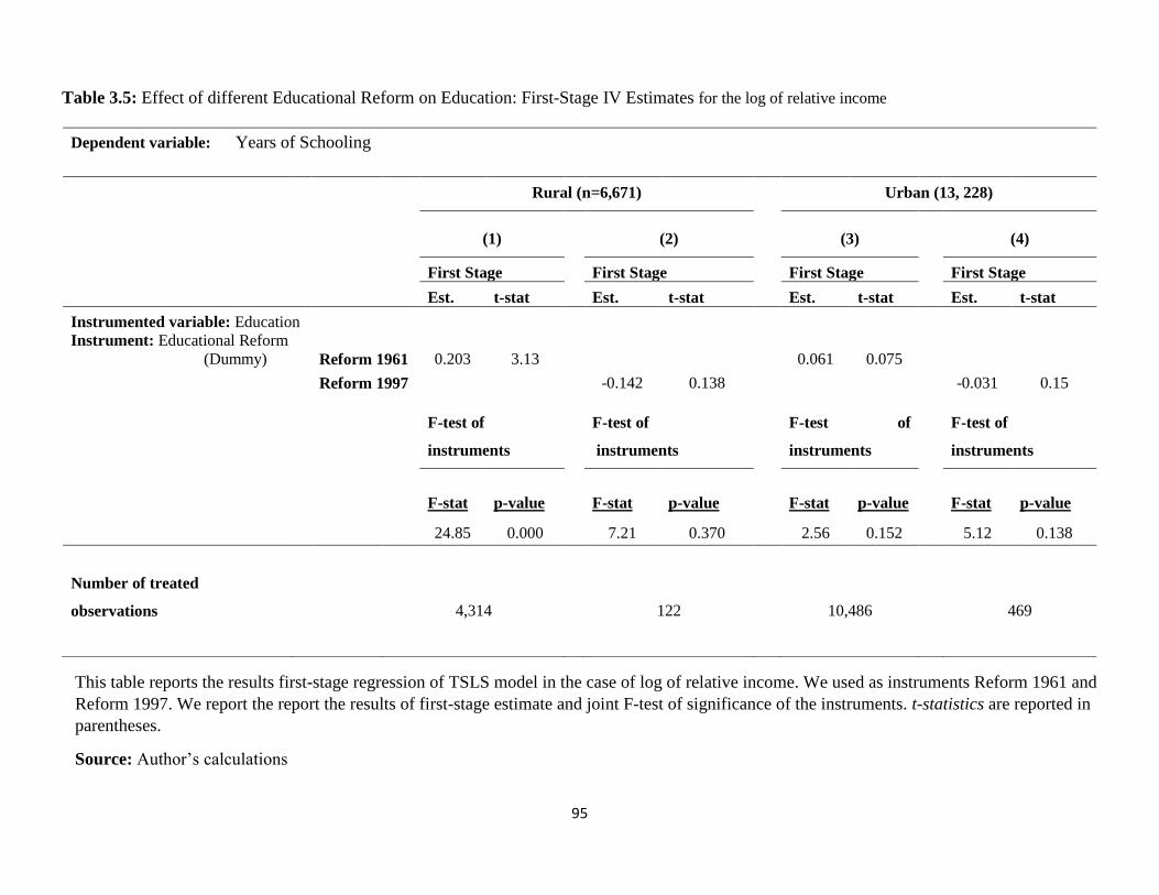
95
Dependent variable: Years of Schooling
Rural (n=6,671)
Urban (13, 228)
(1)
(2)
(3)
(4)
First Stage
First Stage
First Stage
First Stage
Est. t-stat
Est. t-stat
Est. t-stat
Est. t-stat
Instrumented variable: Education
Instrument: Educational Reform
(Dummy) Reform 1961 0.203 3.13
0.061 0.075
Reform 1997
-0.142 0.138
-0.031 0.15
F-test of
instruments
F-test of
instruments
F-test of
instruments
F-test of
instruments
F-stat p-value
F-stat p-value
F-stat p-value
F-stat p-value
24.85 0.000
7.21 0.370
2.56 0.152
5.12 0.138
Number of treated
observations
4,314
122
10,486
469
Table 3.5: Effect of different Educational Reform on Education: First-Stage IV Estimates for the log of relative income
This table reports the results first-stage regression of TSLS model in the case of log of relative income. We used as instruments Reform 1961 and
Reform 1997. We report the report the results of first-stage estimate and joint F-test of significance of the instruments. t-statistics are reported in
parentheses.
Source: Author’s calculations

96
Dependent variable: Years of Schooling
Rural (n=6,671)
Urban (13, 228)
(1)
(2)
(3)
(4)
First Stage
First Stage
First Stage
First Stage
Est. t-stat
Est. t-stat
Est. t-stat
Est. t-stat
Instrumented variable: Education
Instrument: Educational Reform
(Dummy) Reform 1961 0.089 3.95
0.021 0.254
Reform 1997
-0.156 -3.16
-0.109 -3.96
F-test of
instruments
F-test of
instruments
F-test of
instruments
F-test of
instruments
F-stat p-value
F-stat p-value
F-stat
p-
value
F-stat p-value
15.8861 0.000
5.65 0.151
1.242 0.265
8.69 0.224
Number of treated
observations
4,314
122
10,486
469
Number of poor household 960 1,831
Table 3.6: Effect of different Educational Reform on Education: First-Stage IV Estimates for the probability of being poor
This table reports the results second-stage regression of TSLS model in the case of the probability of being poor. The dependent variable is
the log of relative income. We investigate the effect of years of schooling on relative income. z-statistics are reported in parentheses.
Source: Author’s calculations

97
Dependent Variable: The Log Relative Income
Rural
Urban
Second-Stage
Second-Stage
Second-Stage
Second-Stage
Est. z-stat
Est. z-stat
Est. z-stat
Est. z-stat
Years of Schooling 0.073* (-1.94)
-1.66 (-1.52)
0.01 (0.01)
-0.05 (0.15)
Age 0.04** (2.35)
0.08 (2.74)
0.019 (0.45)
0.01 (1.42)
Age-squared -0.0003** (-2.08)
-0.0007 (-2.59)
-0.0001 (-0.30)
-0.0001 (-0.89)
Female 0.07 (1.31)
-0.03 (-0.37)
0.22 (3.49)
0.23 (7.26)
Married -0.33*** (-3.59)
-0.16 (-1.12)
-0.48 (-2.34)
-0.49 (-7.23)
Divorced/Widowed/Separated -0.25*** (-3.02)
-0.13 (-1.09)
-0.39 (-2.06)
-0.39 (-6.01)
Employed 0.058*** (11.10)
0.59 (8.04)
0.67 (5.05)
0.67 (13.46)
Retired 0.067*** (11.22)
0.69 (8.28)
0.58 (9.55)
0.59 (14.84)
Inactive -0.07 (-0.91)
-0.19 (-1.62)
0.06 (0.85)
0.06 (1.55)
This table reports the results first-stage regression of TSLS model. The dependent variable is the log of relative income. We used as
instruments Reform 1961 and Reform 1997. We report the report the results of first-stage estimate and joint F-test of significance of
the instruments. t-statistics are reported in parentheses.
Source: Author’s calculations
Table 3.7: Effect of different Educational Reform on Education: Second-Stage IV Estimates for the log of relative income
(1) (2) (3) (4)

98
Dependent Variable: The Probability of Being Poor
Rural
Urban
Second-Stage
Second-Stage
Second-Stage
Second-Stage
Est. z-stat
Est. z-stat
Est. z-stat
Est. z-stat
Years of Schooling -0.18 (0.95)
0.74 (-1.23)
0.07 (0.12)
0.03 (0.99)
Age -0.009 (-1.01)
-0.03 (-2.25)
-0.005 (-0.26)
-0.01 (-2.39)
Age-squared -0.0006 (0.80)
0.0003 (2.13)
0.0003 (0.16)
0.0001 (2.06)
Female 0.05* (-1.67)
0.01 (0.37)
-0.08 (-2.70)
-0.07 (-4.29)
Married 0.05 (1.18)
-0.04 (-0.62)
0.10 (1.03)
0.05 (1.53)
Divorced/Widowed/Separated -0.01*** (-0.30)
-0.08 (-1.28)
0.06 (0.70)
0.01 (0.55)
Employed -0.031*** (11.59)
-0.31 (-8.44)
-0.33 (-5.03)
-0.30 (-11.15)
Retired -0.039*** (12.89)
-0.40 (-9.55)
-0.38 (-12.73)
-0.37 (-17.70)
Inactive -0.007* (-1.84)
0.003 (0.05)
-0.14 (-3.56)
-0.12 (-5.15)
This table reports the results second-stage regression of TSLS model. The dependent variable is the probability of being poor. We
investigate the effect of years of schooling on relative income. z-statistics are reported in parentheses.
Source: Author’s calculations
Table 3.8: Effect of different Educational Reform on Education: Second-Stage IV Estimates for the probability of being poor
(1) (2) (3) (4)